General Disclaimer

One or more of the Following Statements may affect this Document

This document has been reproduced from the best copy furnished by the

organizational source. It is being released in the interest of making available as

much information as possible.

This document may contain data, which exceeds the sheet parameters. It was

furnished in this condition by the organizational source and is the best copy

available.

This document may contain tone-on-tone or color graphs, charts and/or pictures,

which have been reproduced in black and white.

This document is paginated as submitted by the original source.

Portions of this document are not fully legible due to the historical nature of some

of the material. However, it is the best reproduction available from the original

submission.

Produced by the NASA Center for Aerospace Information (CASI)

https://ntrs.nasa.gov/search.jsp?R=19750022403 2018-06-29T00:07:21+00:00Z

Numerical Simulation of Turbulencet in the Presence of Shear4

0

Prepared from work done under GrantNASA-NgR- 05-020-622

by

S. Shaanan,1. H. Ferz iger,

and

W. C. Reynolds

^oyvluwrgP0

'^ w

• ^ILL9

Report No. TF-6

Ln ^..^W^t-+, t'otin11 =tzo' n 1,r'3a W^^ x WG ^

H ^,... wry .r

, '0C'4 3in ^+

^ ^ Hxnn

r^oLn

HJ N M

LT1 ^

^ HHn

NJ

^ z

r

ti^^.Lj

c 6 ^1 l! N nw

In

.,u,

W0

rn

ThermosiJences DivisionDepartment of Mechanicai Engineering

Stanford University

Stanford, Ca;iforpia

August 1975

i

I ABSTRACT

Numerical computations of three-dimensional time-dependent turbulent

flows are now feasible for three main reasons. The state of the art of

numerical methods for solving the nonlinear Navier-Stokes equations, of

a} turbulent flow modeling for numerical simulations, and of fast computer 1`

hardware have all made three-dimensional simulation a reality. E

The present work deals with the numerical calculations of the largef ^

eddy structure of turbulent flows, by use of the averaged Navier-Stokes

equations, where averages are taken over spatial regions small compared

to the size of the computational grid. The subgrid components of motion

are modeled by a local eddy-viscosity model. A new finite-difference

scheme is proposed to represent the nonlinear averaged advective term E

a/axj (ui u-j ) which has fourth-order accuracy. This scheme exhibits E

- several advantages over existing schemes with regard to the following:

1. The scheme is compact--it extends only one point away in

each direction from the point to which it is applied.

2. it gives better resolution for high wave-number waves

in the solution of Poisson equation.

3. It reduces programming complexity and computation time.

Three examples are worked out in detail.

1. Decay of isotropic turbulence. This problem serves as a

tee''. for the proposed numerical method. Comparison of

numerical results to experimental data (Comte-Sellot and

Corrsin, 1971) shows satisfactory agreement. This brings

us to the conclusion that the numerical method properly

distributes the turbulent energy among different scales,

with proper decay rate.

2. Homogeneous turbulent shear flow. Numerical results con-

firm experimental data given by Champagne, et al (1970)

and Harris (1974) which show departure from isotropy

and growth of length scales in the direction of shear

as the result of the presence of mean shear.

t:

,,

.777777777777777777j..

TABLE OF CONTENTS

Page

ABSTRACT . . . . . . . . . . . . . . . . . . . . . . . . . . . .

jACKNOWLEDGMENTS . . . . . . . . . . . . . . . . . . . . . . . . v

a, TABLE OF CONTENTS . . . . . . . . . . . . . . . . . . . . . . . vi

LIST OF FIGURES . . . . . . . . . . . . . . . . . . . . . . . . viii

. NOMENCLATURE . . . . . . . . . . . . . . . . . . . . . . . . . . x

Chapter 1. INTRODUCTION . . . . . . . . . . . . . . 1

A. General Background . . . . . . . . . . . . . . . . . 1

` B. Objective of Study . . . . . . . . . . . . . . . . . 3

Chapter 2. MATHEMATICAL FORMULATION . . . . . . . . . . . . . . 55

Chapter 3. FINITE-DIFFERENCE FORMULATION . . . . . . . . . . . 10

- A. General Considerations . . . . . . . . . . . . . . . 10

' t B. The Space-Differencing Scheme . . . . . . . . . . . 13

C. The Finite-Difference Poisson Equation . . . . . . . 18

D. The Time-Differencing Scheme . . . . . . . . . . . . 21

Chapter 4. DECAY OF ISOTROPIC TURBULENCE . . . . . . . . . . . 26

A. General Description . . . . . . . . . . . . . . . . 26

B. The Experimental Results . . . . . . . . . . . . . . 27

- C. The Initial Velocity Field . . . . . . . . . . . . . 29

D. Results and Discussion . . . . . . . . . . . . . . . 30

Chapter 5. HOMOGENEOUS TURBULENT SHEAR FLOC! . . . . . . . . . . 39

A. General Description . . ... . . . . . . . . . . . . 39 =

B. Mathematical Formulation . . . . . . . . . . . . . . 40

a. Boundary conditions . . . . . . . . . . . . . . 43

b. Initial conditions . . . . . . . . . . . 43

c. Computational time steps . . . . . . . . . . 43.

C. Results and Discussion . 44.

a. Comparison with experiments . . . . . . . . . . 44

b. Additional numerical results.. 45 '-

c. Pressure-strain correlation Tij . . . 47

Vi

y

y..

p.

l

Page

Chapter 6. HOMOGENEOUS TURBULENT SHEAR FLOW WITH SYSTEMROTATION . . . . . . . . . . . . . . . . . . . . . . .

s60

A. General Description . . . . . . . . . . . . . . . . . 60 z .

B. Mathematical Formulation . . . . . . . . . . . . . . .a

61

C. Results . . . . . . . . . . . . . . . . . . . . . . . 63

D. Interpretation of Results . . . . . . . . . . . . . . 64

Chapter 7. SUMMARY . .. .. ... ... 75

A. Conclusions . . . . . . . . . . . . . . . . . . . . . 75

B. Recommendations . . . . . . . . . . . . . . . . . . . 75

Appendix A. THE FILTERING OPERATOR AND ITS PROPERTIES . . . . . . 77

Appendix B. GENERATION OF INITIAL VELOCITY FIELD FOR ISOTROPICTURBULENCE SIMULATION . . . . . . . . . . . . . . . . 79

Appendix C. THE DISCRETE FOURIER TRANSFORM AND ITS COMPUTATIONALFORM ......................... 84

Appendix D. THE COMPLETE EXPANSION OF THE FILTERED ADVECTIVE TERMFOR THE STAGGERED-MESH CONFIGURATION . . . . . . . . . 86

Appendix E. THE PROGRAM TFC . . . . . . . . . . . . . . . . . . . 95

REFERENCES . . . . . . . . . . . . . . . . . . . . . . . . . . . . 126

iF .

f

vii

?ice

LIST OF FIGURESs

Figure Page

' 3-1 Staggered-mesh configuration in two-dimensions . . . . . . 24

3-2 Comparison of second- and fourth-order Poissonoperators to the exact Fourier transform . . . . . . . . . 25

4-1 Rate of energy decay of isotropic turbulence . . . . . . . 32

4-2 Three-dimensional energy spectra of isotropicturbulence. . . . . . . . . . . . . . . . . . . . . . . . 33

4-3 Dependence of rate of energy decay on numericalconstant. . . . . . . . . . . . . . . . . . . . . . . . . 34

4-4 Dependence of energy spectrum on numerical constant 35

4-5 Rate of energy decay for various model constants . 36

4-6 Energy spectra for various model constants . . . . . . . . 37

4-7 Skewness for different numerical constants . . . . . . . . 38

5-1 Schematic sketch of the homogeneous turbulentshear flow . . . . . . . . . . . . . . . . . . . . . . . . 49

5-2 Mean velocity in a convective frame . . . . . . . . . . . 50

5-3 Turbulence levels in homogeneous shear flow, comparison• with experiment . . . . . . . . . . . . . . . . . . . . . 51

5-4 Shear stress in homogeneous shear flow, comparison with

experiment. . . . . . . . . . . . . . . . . . . . . . . . 52

5-5 Development of turbulent kinetic energy in homogeneousshear flow . . . . . . . . . . . . . . . . . . . . . . . 53

5-6 Development of turbulence levels in homogeneousshear flow . . . . . . . . . . . . . . . . . . . . . . . . 54

5-7 Development of shear stresses in homogeneous shearflow........................... 55

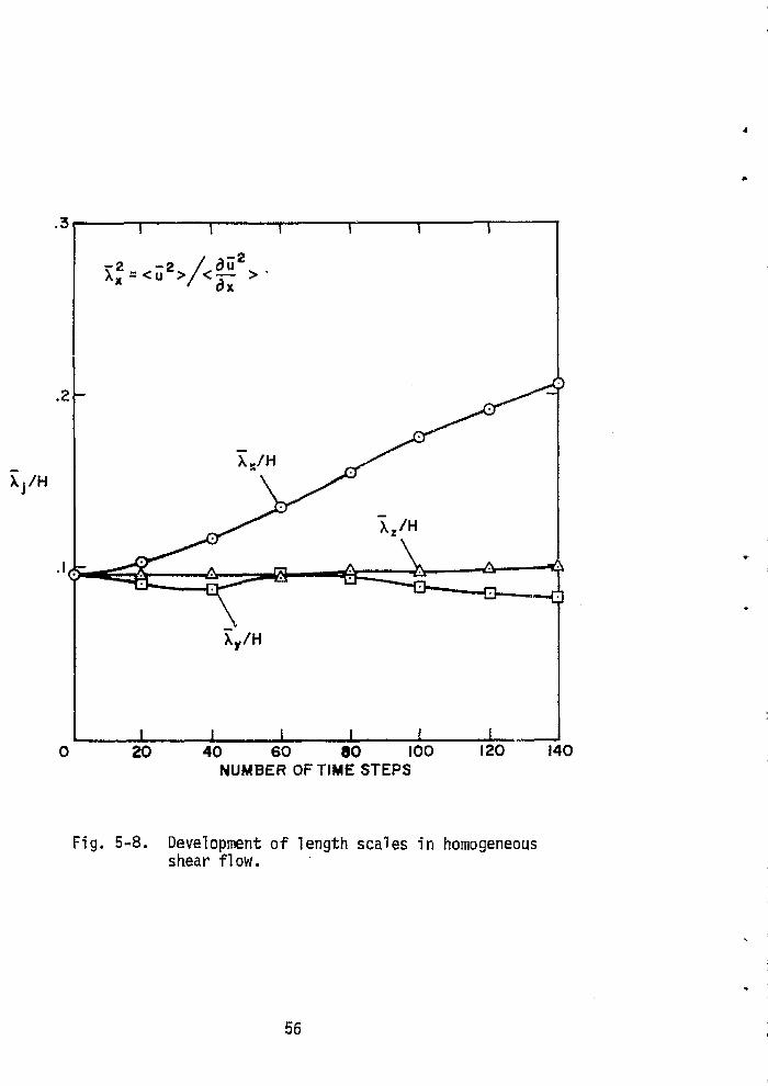
5-8 Development of length scales in homogeneous shear flow . . 56

5-9 Spatial correlations in homogeneous shear flow . . . . . . 57

5-10 Development of pressure-strain correlations inhomogeneous shear flow . . . . . . . . . . . . . . . . . . 58

5-11 Return to isotropy from homogeneous shear . . . . . . . . 59

6-1 Turbulent kinetic energy for different gradientRichardson numbers . . . . . . . . . . . . . . . . . . . . 68

6-2 Shear stresses for different gradient Richardson numbers . 69

' 6-3 Turbulence level of u for different gradient Richardsonnumbers . . . . . . . . . . . . . . . . . . . . . . . . . 70

viii

1

i i.

it !

Page

6-4 Turbulence Ievel of v for different gradientRichardson numbers . . . . . . . . . . . . . . . . . . . . 71

6-5 Turbulence level of w for different gradientRichardson numbers . . . . . . . . . . . . . . . . . . . . 72

6-6 Mixing-length ratio versus gradient Richardson number.Data from Johnston (1974) . . . . . . . . . . . . . . . . 73

6-7 <U > 1/2 versus gradient Richardson number at varioustimesteps . . . . . . . . . . . . . . . . . . . . . . . . 74

S-I Coordinate system for decomposition of u . . . . . . . . 83

.,

s L

x

f

1.

ix3

NOMENCLATURE

English letters

a = a constant defined by Eq. (6-44)

a 1 ,a2 ,a3 ,a4 = constants defined by Eqs. (B-13) and (B-14)

A = Rotta's constant defined by Eq. (5-28)

b anisotropy tensor defined by Eq. (5-30)

c = turbulence model constant

cl ,c2 = constants defined by Eq. (6-26)

O = isotropic dissipation

dsgs= subgrid scale dissipation

E = three-dimensional energy spectrum

f = a function

f = Fourier transform of f

g = filtering function defined in Appendix A

g = Fourier transform of g

h = mesh size

R = length of computational box

i,j,k = indices describing spatial locations on a mesh

I,J,K = computational indices

k,ki = wave-number vector

k;k! = modified wave-number vector defined by Eq. (4-13)

k = magnitude ofk

N2 = k k i )

K = eddy-viscosity coefficient defined by Eq. (2-13)

' Q = mixing length

L = number of time steps

x

m spatial frequency (m k/2ir)

M diameter of bars of the isotropic turbulence generator

N number of mesh points

CCourant number

n index

p turbulent instantaneous pressure

P instantaneous pressure

P* modified instantaneous pressure

p Fourier transform of p

q W RHS of Poisson equation (2-18)

q Fourier transform of q

2q /2 = turbulent kinetic energy

r = rotation defined by Eq. (6-39)

L.ri= separation vector

r = rotation tensor of turbulence

aid rotation tensor of instantaneous field

R = correlation tensor

= tensor defined by Eq. (6-36)

Re = Reynol ds number

Ri gradient Richardson number

s strain rate defined by Eq. (6-39)

s RHS of momentum equation (2-17)

S r rate-of-strain tensor of turbulence

rate-of-strain tensor of instantaneous field

S w skewness

t time

t,ti = reference vector defined in Appendix B

'TiJ

= pressure-strain correlation tensor

u,ui = instantaneous turbulent velocity vector

U,U i = instantaneous velocity vector

U,V,W = instantaneous turbulent velocity components

U,V,W = instantaneous velocity components

Uo = mean velocity

U = centerline velocity

x,xi = position vector

x,y,z = Cartesian coordinates

R = stretched x coordinate

Greek symbols

a = numerical constant defined by Eq. (3-19)

= a constant defined by Eq. (6-2)

Y = a constant defined by Eq. (3-2)

r = mean velocity gradient

si,j = Kronecker delta

filter width

c i j k= unit alternating tensor

= angle defined in Fig. B-1

n = random number

6 = angle defined in Fig. B--1

A = Taylor microscale

V = kinematic viscosity

' p = density

piJ= tensor defined by Eq. (6-30)

xii

R i

ir

stress tensor defined by Eq. (2-9)

Ti,7= shear tensor defined by Eq. (2-10)

= angle defined in Fig. B-1

f^ij

= spectrum tensor

angular velocity vector

vorticity vector !r"°`

Other symbols

DO : D+^D„

4Do' 4D}' 4D-= finite-difference operators for first derivative

. D^ = finite-difference operator in jth direction

L) = vector

(^) = average according to definition given by Eq. (2-4)'=v

(') = subgrid scale component +

< > i ^ = averages over planes defined by ij coordinates

< > = averages over the entire volume

* = conjugate

^r = convolution

FT = Fourier transform

DFT = discrete Fourier transform

F

FFT = fast Fourier transform

RHS = right -nand side

RMS = root mean square

CFTC = Champagne, Harris, and Corrsin

f^

xi i i

7T ^^

6 CHAPTER I

INTRODUCTIONi

A. General Background

In recent years, because computers have become faster and larger, x °.

a new approach in handling turbulent flow simulations has emerged. This

is a three-dimensional, time-dependent numerical simulation of the large-

scale structures of turbulent flows. In this approach, a variation of

an old idea is used; one applies a spatial averaging operator to the

equations of motion. The averages are taken over regions small compared:

to the size of the computational domain, and the subgrid components of

motion are modeled with a local eddy-viscosity coefficient.

One of the first successful attempts in using this approach was

Deardorff's in a numerical study of three-dimensional turbulent channel

flow at high Reynolds numbers (Deardorff, 1970). The main purpose of

his work was to extend earlier work by meteorologists (Smagorinsky, 1''

et al., 1966; Leith 1966), who used these methods in calculating the

general circulation of the atmosphere in two dimensions, to fully three-

dimensional turbulence for a laboratory problem. Other works of interest

that followed this approach are Deardorff (1972) and Schumann (1973).

The numerical discretization techniques that have been used in the

mentioned works and in other investigations fall basically into two

categories, namely, spectral methods and real-space methods. Spectral

methods, which deal with the transformed equations in Fourier space, are

the most accurate methods. However, when applied to the Navier-Stokes

equations, they exhibit a major drawback. The nonlinear advective terms

appear as convolution sums, and have to be treated in quite a complicated

way in order to avoid aliasing errors. Another difficulty is that the I;

method is capable of handling only geometrically simple problems with ^-

periodic boundary conditions. Detailed descriptions of the spectral

methods can be found in the work of Orszag and co-workers (Orszag, 1969,

} 1971 a,b; fox and Orszag, 1973; Orszag and Patterson, 1972).

1 !^

Real-space methods use finite differences for discretization in

various forms. The most popular methods are second-order schemes, which

have particular conservation and stability properties, as will be dis-

cussed later. The main contributions to these methods can be found in the

works of From (1963), Harlow and Welch (1965), Lilly (1965), Arakawa^k: l

(1966), Williams (1969), Deardorff (1970), and others. Although finite

difference methods are inferior to spectral methods with respect to accuracy,

they have the advantage of not being restricted to simply shaped regions

and periodic boundary conditions, and this generality makes them suitable

to flows of engineering interest, i.e., flows which contain wail-bounded

as well as boundary-free regions.

Only a few three-dimensional time-dependent flow simulations have

been reported so far. The main reason is the restricted capability of

computers in the past, in terms of speed and capacity. Even today, with

the use of the largest available computer (CDC 7600), a 32 3 mesh-point

problem is the upper limit for a core-contained program, provided the

simplest periodic boundary conditions are used, and an average simulation

consumes about half an hour of running time. The use of peripheral

equipment, such as tapes, discs, or other mass memory and storage, com-

plicates the operation significantly in terms of programming and turn- ;.

around time.

The reported works include those of Deardorff (1970) and Schumann

(1973), simulating the channel flow, using 24xl4x2O and 64x32xl6 mesh

points, respectively, by finite-difference methods; of Orszag and Patterson

(1972), simulating three-dimensional homogeneous isotropic turbulence,

using 323 mesh points by spectral methods; and of Kwak, et al. (1975),

simulating an isotropic turbulence and a pure strained turbulent flow,

using 323 and 163 mesh points, respectively. Clark (ongoing Ph.D. re-

search, Stanford University) is working on turbulence modeling, using a

643 mesh-point program. It is hoped that a 64 3 mesh-point problem will

be standard for the ILLIAC IV computer, which will be operational in

the near future.

2

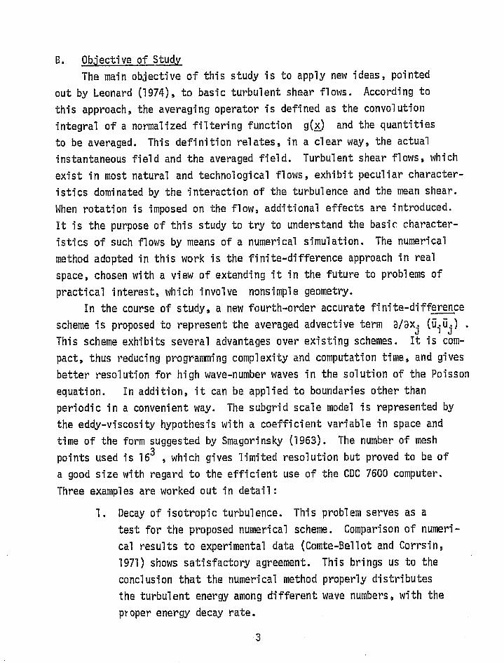
B. Objective of Stud

The main objective of this study is to apply new ideas, pointed

out by Leonard (3974), to basic turbulent shear flows. According to

this approach, the averaging operator is defined as the convolution

J integral of a normalized filtering function g(x) and the quantities

to be averaged. This definition relates, in a clear way, the actual

instantaneous field and the averaged field. Turbulent shear flows, which

exist in most natural and technological flows, exhibit peculiar character-{

istics dominated by the interaction of the turbulence and the mean shear.

When rotation is imposed on the flow, additional effects are introduced.

It is the purpose of this study to try to understand the basics character-

istics of such flows by means of a numerical simulation. The numerical

method adopted in this work is the finite-difference approach in real

space, chosen with a view of extending it in the future to problems of

practical interest, which involve nonsimple geometry.

In the course of study, a new fourth-order accurate finite-difference ty- .

scheme is proposed to represent the averaged advective term a/axj (ui uj ) _ry

This scheme exhibits several advantages over existing schemes. It is com-

pact, thus reducing programming complexity and computation time, and gives

better resolution for high wave-number waves in the solution of the Poisson

equation. In addition, it can be applied to boundaries other than

periodic in a convenient way. The subgrid scale model is represented by

the eddy-viscosity hypothesis with a coefficient variable in space and

time of the form suggested by Smagorinsky (1963). The number of mesh

points used is 16 3 , which gives limited resolution but proved to be of

a good size with regard to the efficient use of the CDC 7600 computer.

Three examples are worked out in detail:

1. Decay of isotropic turbulence. This problem serves as a

test for the proposed numerical scheme. Comparison of numeri-

cal results to experimental data (Comte-Ballot and Corrsin,

1971) shows satisfactory agreement. This brings us to the

conclusion that the numerical method properly distributes

the turbulent energy among different wave numbers, with the

proper energy decay rate.

3

2. Homogeneous turbulent shear flow. Numerical results confirm

experimental data given by Champagne, et al. (1970) andY:

^. Harris (1974) which show departure from isotropy and growth 4

of length scales in the direction of shear as the result of

^ the presence of mean shear.

3. Homogeneous turbulent shear flow with system rotation.

Numerical results show clearly the effect of rotation on

the stability of turbulence, as was shown experimentally

by Johnston (1974) .

-. The numerical simulation of the model equations of turbulence given in

this work proves to be a convenient way for extracting useful information

on the physics of a variety of basic turbulent flows, and extends con-

siderably the existing experimental data for these flows.

s

.. ikff

4

f

CHARTER 2

MATHEMATICAL FORMULATION

The basic equations for the following analysis are the Navier-Stokes

equations for an incompressible fluid:

au i ('x,t)`^ -

a( 11{^.^ i uj } - - ^- v

p a-^p

a2uiT1,2,3 {2-l)aX^axat axe j

Du axi = 0 (2-2)

Q

where ui , p , p , v are the velocity, pressure, density, and kinematic

viscosity, respectively. The summation convention is implied.

In principle, any incompressible flow'is completely determined by

the solution of these equations, provided boundary and initial conditions

are specified. Actually, analytical solutions exist only for a few

special cases, and one must resort to approximate solutions, by assuming

steady-state behavior, by assuming two-dimensionality, or by dropping

terms which are estimated to be small by an 'order of magnitude ; analysis,

etc., or one must rc-,ort to numerical methods. One of the major diffi-

culties arising in numerical calculations of turbulent flows is the widerange of length scales presented in the flow. Any numerical method is

limited by its own nature, namely, it can represent only a finite range

of length scales. The maximum wave.-number that can be resolved on a

grid of points a distance h apart is kmax = 7r/h, and "honest" numerical

calculation of turbulence for high or even moderate Reynolds numbers,

requires a number of mesh points which is far behind the capability of

today's computers.

As an example, consider the problem of grid-generated isotropic

turbulence (Comte-Bellot, and Corrsin, 1971). The reported Reynolds

number based on Taylor microscale X and RMS turbulent velocity level

is in the range of Re r-60 to 70. The Kolmogorov wave-number, at which

molecular dissipation occurs, is k = 34 cm -1 . The wave—number which

corresponds to the location of the energy peak in the three-dimensional

5

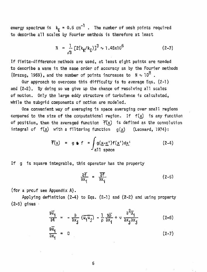
N = 1 [ 2 (kK/ kE ) I3 ti 1.45x105

V3i

(2-3)

of _5Taxi y axi

(2-6)

n'

energy spectrum is kE = 0.5 cm-1 . The number of mesh points required f

to describe all scales by Fourier methods is therefore at least

a

If finite-difference methods are used, at least eight points are needed

to describe a wave in the same order of accuracy as by the Fourier methods

(Orszag, 1969), and the number of points increases to N u 103

Our approach to overcome this difficulty is to average Eqs. (2-1)

and (2-2). By doing so we give up the chance of resolving all scales

of motion. Only the large eddy structure of turbulence is calculated,

while the subgrid components of motion are modeled.

One convenient way of averaging is space averaging over small regions

compared to the size of the computational region. If f(x) is any function

of position, then the averaged function f(x) is defined as the convolution

integral of f(x) with a filtering function g (x) (Leonard, 1974):

(x} = g * f^-f

al

g( x-x')f (x')dx' (2-4) .

l space

If g is square integrable, this operator has the property

(for a prol.^f see Appendix A).

Applying definition (2-4) to Eqs. (2-1) and (2-2) and using property

(2-5) gives

aui a a2uiat - - axi N uj -

lp @1X1

+ V ax.ax. (2-6)

au -ax -

D (2-7)

6

r

Tij-(aij - 3 okkSij) (2-10)

b The difference between the local velocity u and its averaged value

ui is due mostly to the high wave-number part of the flow which cannot

be included directly in the computations. If we set u3 = u i -- Ti and

substitute into the term (u i uj , we obtain

Ui ^,^ = M. + U!u + u i ul + u— u (2-8)

The last three terms in Eq. (2-8) represent the subgrid scales and must

be modeled in terms of the resolvable part of the velocity field, in order

to close the equations. A convenient way of modeling these terms is by

means of a local eddy-viscosity model. We define a stress tensor

u! u + Ui U1. + 77 (2-g)

We further subtract the trace from aij to define the stress tensor of

the subgrid scales as

Substitution of Eq. (2-10) into Eq. ( 2-6) gives

2Bui

at T - ax• ( Ui uj ) - ax^ ( p Ip + l/3 6kk) + ax^ T i j + " ax.ax:

(2-11)

The term (p/p + 1/36kk) is a generalized pressure and will be designated

simply as p from now on.

Tij is modeled by an eddy-viscosity hypothesis,

Tij - 215iJ (2-12)

whereau au

Y.

+

s^ -- axl a—x (2-l) x

A

K is a proportionality constant with the dimensions (length)2/time.

7

Following Smagorinsky (1963), K is defined to be proportional

to the magnitude of the local rate-of-si'^ain tensor of the large structure.

To make K dimensionally consistent, a length scale should be introduced

into the definition, and if we take it to be the mesh spacing h , then

K - (ch)2(2sij sij)l

/2 (2-14)

Ifs....,...,_

Lilly (1966) estimated the model constant to be c = 0.22 by assuming

that the wave number 7r/h lies in the inertial subrange in an isotropic

turbulence problem. However, Deardorff (1970), in his channel flow

simulation, has found that the constant must be modified downward by

about 50%. Later in this work, this constant will be assessed, based on

our numerical results.

Another model, which is similar, at least in the numerical complexity,

to the above model is the vorticity model, where K is proportional to

the magnitude of the local vorticity:

K = (ch) 2 (wiwi ) 1/2(2-15)

where wi is given by _

auk a

W = eijk Fx7 (2-16)

In a recent simulation of isotropic turbulence (Kwak, et al., 1975), bothmodels were used and no major differences were found. Based on this

experience, we shall use Smagorinsky's model throughout this work.

Since dissipation due to molecular interaction is much smaller than

dissipati on due to turbulence, the term a ui /a xj axj appearing in Eq .

(2-6) will be excluded. To maintain incompressibility, we shall use

a Poisson equation instead of Eq. (2-7). This equation is derived by

9d

,a

j axiaxj

axe ax i - axi axi (ui'^i ) ^' ax-2

axi ^i ( 2 "^ s}

r#

,F

4

F

CHAPTER 3

FINITE-DIFFERENCE FORMULATION

A. General Considerations

The major difficulty arising in the solution of the averaged set of

equations formulated in Chapter 2 is treatment of the term a/aX, (u;uj).

One approach suggested by Leonard (1974) is first to expand u i uj in

a Taylor series around If a symmetrical filter is used in the

definition

axj (u;ua) = axj 9%X-X') ui (x') uj (x') dx` (3-1)

the result is

2 2

a s (u i uj ) = axj (ui uj) + A axa as (uiuj) + O(A4) (3-2)

Y,i

where A is the averaging length scale, and the constant y depends on

the particular filtering function g(x) . For example, a Gaussian filter

defined by

I/2 3

9(x) _vw)

exp(-6 12LI /A ) (3-3)

gives the value y = 24 . The second term of the RHS of Eq. (3-2) is

the so-called "Leonard term." As we shall see, this term contributes

substantially in controlling the proper energy transfer among the eddy

scales, and therefore should be accounted for in the numerical calculations.

In general, any finite-difference scheme which is applied to the

incompressible Navier-Stokes equations must have certain integral con-

servation properties, if longtime integrations are required. The minimum

requirements are mass, momentum, and energy conservation, which means that

in the absence of dissipation and truncation errors caused by the time-

differencing scheme, the method should have the following properties:

^ y

t > d

10E j:

t:

is

E(D) i ui = 0 (3-4)

8 F' ui " 0 i= 1 ,2,3 (3-5)p

^F F uiui - 0 (3-6)

P

where P

is the sum over all mesh points in an infinite (or periodic)

domain, and M 4 . is the finite-difference operator for the first

derivative in the i th direction. glass conservation is controlled by

a Poisson equation, and a discussion of this property will be given in

section C of this chapter. It can be shown easily that conditions (3-5)

and (3-6) impose the following requirements on the advective term:

E

(D) j (ui ui ) = 0 i = 1,2,3 (3-7)

F u i (D) i ( u i ui ) = 0 (3 -8)

In the past, two common second-roder schemes have been used to •

implement these requirements. The first one uses a regular mesh configura-

tions where the variables u i ,p are defined in the same location. This

scheme is given by

3xj (uiui) IT 1 ( 3-9)

(uiu^} + ui ( Do )^u^ + uj ( Do ),ui + 0(h2)( 3-9)

where (D0 ) J is the central-difference operator defined by (one dimension)

^l

The second method uses a staggered-mesh configuration with the variables

u i , p defined as shown in Fig. 3-1. We will give the formu'€is for this

case later.

It was shown by Leonard (1974) that if the averaged equations are

used and the term a/axj (ui uj ) is expanded as in Eq. (3-2), the !.eonard

term is nonconservative, and preliminary estimates have shown that this

term has a significant part in energy extraction from large scales. How-

ever, the term a/axj (ii i uj ) is conservative. Since the Leonard is of0(h 2), a straightforward approach to retain it in a numerical calculation

is to use a fourth-order finite-difference scheme for the term a/ax j (uiuj)

and a second-order scheme for

A2 a 2 a

Y axZaxk ax (u i ^j ) .

One possible realization which maintains properties (3-7) and (3-8) for

the term a/axj (ui uj ) is as follows.

The fourth-order scheme for the term a/axa (u.i uj ) is obtained by

Richardson`s extrapolation (Richardson, 1927). By applying the operator

defined by Eq. (3-9) to a mesh with 2h spacing, and then combining the

scheme derived for h with that for 2h with weights 4/3 and -1/3

respectively, we have

a (u u)= 4 1[(D) (uu)^-^(a) u +u(0) uaxji j 3 2 o j,h i j i ( D

o ) j j j o j,h i

1 2 [(D°). 2h(u i u ,- ) + u i (Do ) j,2h uj + uj(Oo),a ,2h ui] +0(h4)

(3-11)

In order to get the Leonard term, the Laplacian a 2/ axA MY, is approximated

by the second-order operator (D +D - ) i , where for one dimension we have

(D+ ) un = ( un+l - un )/h (3-12)

(D- ) un = (un - un -1)/h (3-13)

(D+D- ) un = (un+l - 2un + un -1 )/h2 (3-14)

s,

12

The finite-difference scheme for the Poisson equation in this realiza-

tion is given by

(40o4Do ) x k (4po4Co )y

+ (4go4'o )x l p y q (3-15)

woere 4D0

is the fourth-order central-difference operator defined by

(one dimension)

'' + 8u u }/12h (3-16)( 4`'o^ un - (-un+^ n^-1 - 8u +n-1 n-2

This method has been used successfully in a recent numerical simulation

of turbulence (Kwak, et al., 1975). However, it has two major drawbacks:

1. The scheme extends four points in the major directions

away from the point to which, it is applied. This makes

the method inconvenient to apply in problems with boundary

conditions that are not Periodic..

2. It gives poor resolution for high wave-.lumbers in the solu-

tion of the Poisson equation, as we shall see in section

C of this chapter.

In the following, a new finite-difference scheme is proposed, which

removes some of these difficulties. The scheme is compact, it uses in-

formation from adjacent points only, and the Poisson solver follows the

exact solution more closely. In addition, a reduction in computation

time is achieved.

B. The Space-Differencing Scheme

Consider the one-dimensional advective term

Ux(uu} - UT (uu) y 77 ax

(uu) ( 3 -17)dx

If we choose A2/-Y = h2/6 , we can approximate this term by the central-

difference operator Do with fourth-order error term:

fi

13

2

dx (55) + 6

2d x (uu} = Do (uu) + 0(h4 ) (3-18)

dx

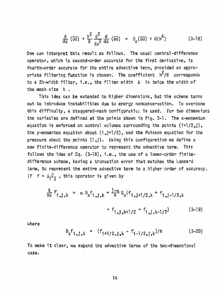
One can interpret this result as follows. The usual central-difference

operator, which is second-order accurate for the first derivative, is

fourth-order accurate for the entire advective terms provided an appro-

priate filtering function is chosen. The coefficient h 2/6 corresponds

to a 2h-width filter, i.e., the filter width A is twice the width of

the mesh size h .

This idea can be extended to higher dimensions, but the scheme turns

out to introduce instabilities due to energy nonconservation. To overcome

this difficulty, a staggered-mesh configuratic,,< is used. For two dimensions

the variables are defined at the points shown in Fig. 3-1, The x-momentum

equation is enforced on control volumes surrounding the points (W /2,j),

the y-momentum equation about (i,jk1/2), and the Poisson equation for the

pressure about the points (i,j). Using this configuration we define a

new finite-difference operator to represent the advective term. This

follows the idea of Eq. (3-18), i.e., the use of a lower-order finite-

. difference scheme, having a truncation error that matches the Leonard

term, to represent the entire advective term to a higher order of accuracy.

If f = ui uj , this operator is given by

Tx i,j,ka

Dxfi,j ,k + l4a Dx(fi,j+1/2,k + fi,j-1/2,k

f fi,j,k+1/2 + fi,j,k-1/2)

(3-19)

where

Dxfi,j,k - (fi+1 /2,j,k - fi-1/2,j,k) /h (3-20)

To make it clear, we expand the advective terms of the two-dimensional

case.

14

.r

_E

,a

x-momentum equation:

a (uu} aD (uu) + 1-a Uax i+l/2,j x i+1 /2,j 2 x {uu} + (uu)i+l/2,j+1/2 i+1/2,j-1/21

(3-21) !

a (uv} - aD, (u-v) + 1-a D ^(uv} + (uv} (3-22)ay 2,j ^' i +1/ 2 ' j 2 Y i+l ,j i s jy-momentum equation:

i

a {vu ) i ,j+l/2 - aDx(v- u}i ^j+1 / 2 + 1 2A Dx[(vu) ', ^ j+ 1 + (vu}i ^j] ( 3-23)

ay i,j+1 / 2 y i,j+1/2 . 2 y i+1/2,j+1/2 i -112,j+1 12

(3-24)

Since in the staggered-mesh configuration not all variables are availablef

at points where they are needed, averages are to be taken from adjacentv

points. For example,

(5v)i+l /2J+1/2 =

(5 1 +1/ 2,j + 5i +1/2, j+1 ) (v i 9j+1/2 + vi +1 j+1/2)/4

(3-25)

Using these averages in the proposed scheme, and expanding in a Taylor

series about the points to which the scheme is applied, we obtain the

following (two representative terms are given; other terms can be obtained

Y):

r'15

finite-difference scheme of ax (u) 2uux +

2

+ hL65xuxx + 4uuxxx + 3(1-a)(UUXYY

+ 55xzz

+ uxuyy + Uxazz + UYUxY + EZUX,)] +a(h4)

(3-26)

finite-difference scheme of +

y (uv) navy + uyv

2

+ ^2 [(3a+1)(2 oy^xx + 2 u^xxy + 2 uY^YY

+ 1 uvYYY + 2 uYYY^ + 3 Uyyvy)

+1( 1-a)(uxY^ + 5x + uxxyv + Exx^Y

+ uyvzz + uvzzy vzuyz + uzvyz v^izZy

1 ^j 9

+ v Uzz )I + 0(h4)(3-27)

The exact expansion of the desired terms is

2

ax (uu) 25a + [6 5XGXX + 2uuxxx

+ 255xyy + 2uuxzz

+ 25x5yy + 2ux5Zz + 25y5xy + 25z5Xz] `3-28)

T

16

E ^^

+uv +u v+3u v +2u v +2uv +u vyyy yyy yy y xy x x xy xxy

+ uxxvy + uyvzz + uv-zzy + 2v z5yz + 25zvyz + via

zzy + vy zzI

(3-29)

By comparing the finite-difference scheme, Eqs. (3-26) and (3-27), to the

exact expansion of the advective term, Eqs. (3-28) and (3-29), it can be

seen that for a 1 all terms of the finite-difference scheme occur in

the exact expansion with different multiplicative constants. In other

words, the proposed scheme contains a Leonard term, with filtering proper-

ties which depend on the numerical constant a . it is impossible to

find a simple expression for this equivalent filter in terms of a

but one can put upper and lower bounds for A2 /y for any value of a .

For example, if a = 1/3, the scheme represents a filter with

h2 A2 h224 < 7 ` 7- '

or, in terms of the Gaussian filter, the width of the filter is between •

h and 2,/2 h with most of the terms corresponding to A = J2 h . When

a = 1, the scheme reduces to the staggered-mesh scheme first introduced

by Fromm (1963) .

Other terms appearing in the governing equations are finite-differenced

in the usual way, for example,

)i + .+ - P. /h (3-30)1/2.^,k

W (P l,3,k i ,j k)

The eddy-viscosity coefficient K is evaluated at the same place as the

pressure p (see Fig. 3-1).

The complete expansion of the filtered advective term according to

+ Eq. (3-19) is given in Appendix D.r

FiF

E

3E^

{

_ 17

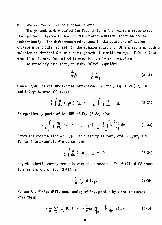
C. The Finite-Difference Poisson Equation

The present work revealed the fact that, in the incompressible case,

the finite-difference scheme for the Poisson equation cannot be chosen

independently. The difference method used in the equations of motion

dictate a particular scheme for the Poisson equation. Otherwise, a nonstable

solution is obtained due to a rapid growth of kinetic energy. This is true

even if a higher-order method is used for the Poisson equation.

To exemplify this fact, consider Euler's equation.

du i 1 .P (3-31)r - p axi

where d/dt is the substantial derivative. Multiply Eq. (3-31) by ui

and integrate over all space:

2 dt (ui u i ) dx = - ^ u i ^ dx (3-32)

Integration by parts of the RHS of Eq. (3-32) gives

au

i adx (uip)

A pex dx (3-33)

p °'

Since the contribution of u i p at infinity is zero, and au i /2xi = 0

for an incompressible fluid, we have

1 f d(u i u i ) dx _ 0 (3-34)

or, the kinetic energy per unit mass is conserved. The finite-difference

form of the RHS of Eq. (3-32) is3

t :,

- u•(D•p) (3-35)

We use the finite-difference analog of integration by parts to expand

this term:i4

- u•1 )( D P) -- - (u.p + 1 p(D.u.) (3-36)P p 7 Co p [

I ez`

18

I

f

Each term in the RHS of Eq. (3-36) is equal to zero and energy is d

conserved.

The use of integration by parts in a finite-difference form is con-

sistent only if the operators of the expressions (D i p) and (Diui)

are identical. Therefore, a choice of an operator for the pressure-

gradient term (D i p) in the equations of motion forces us to choose

the same operator for the divergence term (D i u i ), which brings us to

the conclusion that the proper Poisson operator should be in the form

32--. ti Di Di (3-37)axi

To derive the Poisson operator for a staggered-mesh, one additional

fact has to be taken into account, namely, that the variables u are

out of phase by half the mesh size relative to the pressure p . Since a

computational cell (see Fig. 3-1) is defined as

u(I,J,K) = ui}1/2,j,k

v (I,J,K) = vi,j+1/2,k(3-38)

w(I,J,K) = wi,j,k+1/2

p ( I .J ,K) = P i ,3 sk

we find that a second-order operator for ^p/Dx , which appears in the

equations of motion, is given by

p1i ru [P(I+I,J,K) - p ( I ,J ,K)I /h = (D+ ) x p (3-39)

+l/2,j,k

and a second-order divergence operator for au/8x is given by

(29). ti [u(I,J,K) - u( I-1,J,K) /h = (D_) xu (3-40)

19

r --77

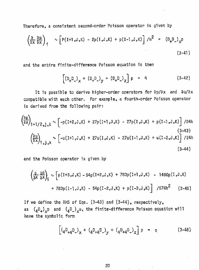
3Therefore, a consistent second-order Poisson operator is given by

tiaaaxx^ ti [P(1+1,j,K) - 2 p ( I ,J ,K) + p(I-1,J,K)I /h2 = (D+D_)xp

i

(3-41)

and the entire finite-difference Poisson equation is then

l

[(D+D_) x + (D+D_)y + (D+D - ) zI p = q

(3-42)

r.

It is possible to derive higher-order o perators for ap/ax and au/ax

compatible with each other. For example, a fourth-order Poisson operator

is derived from the following pair:

lax i+l/2^3^k ti -ptI+2,J,K) + 27p(I+1,J,K) - 27p(I,J,K) + p(I-1,J,K)1 /24h

(3-43)

au ti [-u(I+1,J,K) + 27u(I,J,K) - 27u(I-I,J,K) + u(I-2,J,K)l /24hax i,j,k

(3-44)

and the Poisson operator is given by

^a ^7 , [p(I+3,J,K) -54p(I+2,J,K) + 783p(I+1,J,K) - 1460p(I,J,K)

+ 783p(I-1,J,K) - 54p(I-2,J,K) + p(I-3,J,K)^ /576h 2(3-45)

If we define the RHS of Eqs. (3-43) and (3-44), respectively,

as (4D+)xp and (4D_) xu, the finite-difference Poisson equation willhave the symbolic form

[(4D +4 D_) x + ( 4D+40- )y + ( 4D+4D - ) ZI p = q (3-46)

3

20

,I

In order to assess the relative accuracy of these operators, it is

customary to compare them with the exact Fourier transform. Fourier

transforming the various one-dimensional finite-difference Poisson operators

and the continuous operator 92/Bx2 and plotting the transformed coefficients

versus the nondimensional wave number kh , Fig. 3-2, one can see the

relative distortion introduced in the solution by the different schemes.

The fourth-order regular-mesh curve represents Eq. (3-15). As is seen,

the staggered-mesh configuration shows a substantial advantage over the

regular mesh. For kh > 0.25 the difference between the fourth-order

regular mesh and the exact Fourier method tends to grow sharply, while

the staggered-mesh curves trace the exact solution much more closely.

In this work, we shall use the second-order Poisson operator on

a staggered mesh. Although inferior to its fourth-order counterpart, it

has the advantage that the scheme extends only one point away from the

point to which it is applied.

The actual solution of the Poisson equation is by means of a direct

method. The discrete Fourier transform of Eq. (3-42) is given by

4 sing 7r7 } sin ^ + sing Trk

N N l

N N Ia p r g j 1 9,7,k=--•,.. ,2 -

(3-47)

To obtain p , we first transform q into q then solve for p accov ding

to Eq. (3-47), and finally inverse transformp to obtain p . The fast

Fourier transform algorithm (FFT) is used in the numerical realization.

For further details of 't FT methods see Cochran, et al. (1967) and

Appendix C.

D. The Time-Differencing Scheme

The basic equations of motion can be reduced to the form

Du i _at

si (3-48)

where s i is a complicated nonlinear function evaluated at each time

step for every mesh point, by one of the methods described in the previous

sections.

21

i

A

This equation, which is parabolic with respect to time, can be solved

by methods which are analogous to methods for first-order ordinary

differential equations. The existing methods can be classified according

to the following criteria: accuracy, stability, one step or multistep,

implicit or explicit methods. For extensive treatment of this subject

the reader is referred to the book by Gear (1971).

For the present problem two additional criteria were considered,

namely, the number of evaluations of s i per time step, and the amount

of storage required. These features are characteristic of problems of

large volume and long computation time.

Two commonly used methods, which are second-order accurate and

require only one function evaluation per time step, are the leapfrog and

the Adams-Bashforth methods. Both are multistep methods and require

storage for two time steps. The leapfrog method is given by

ui (nfl

= ui (n-1) + 2 At s i (n) (3-49)

with truncation error

a3--

6 At

3(3-50)

DO

and the Adams-Bashforth method is given by

u (n+l) u.(n) + At(3s^ n) - s (n-1) )/2 (3-51)7 7 ^ 7

with truncation error

3--

12 Atz

a u ^ (3-52)

at

A linear-stability anal ysis shows that the Adams-Bashforth method is more

stable than the leapfrog method (Lilly, 1965).

}

i

22

UmaxAtNc - Ax

(3-53)

In this work we use the Adams-Bashforth method. The time stepe

is chosen to give a Courant number of N c = 0.25 where

_s

dmax is the magnitude of the maximum velocity appearing in the problem.

c

:V

COMPUTATIONALO P,K •U CELL (I,J)

l •VI VI, j+,/2 1! 1

1 ^

•P h •U •Pi,1 •P •U

sV

FLUID ELEMENT

•P

Fig. 3-1. Staggered mesh configuration in two-dimensions.

C.

f

24

5

4th ORDERSTAGGERED MESHEQ. (3-46)

4FOURISR

3N

k 2nd ORDER1

STAGGERED MESH2

EQ. (3-42)

41h ORDERREGULAR MESHEQ. (3-15)

1 I ^0 .125 .250 .375 .500

kh

Fig. 3-2. Comparison of second and fourth order Poissonoperators to the exact Fourier transform.

25

t'ir

CHAPTER 4

DECAY OF ISOTROPIC TURBULENCE

A. General Description

f

The decay of isotropic trubulence has been chosen as the first

problem for numerical simulation. A random-velocity field which satisfies

certain correlation and energy properties is specified within a box, and

the evolution of this field is observed at later times. This problem,

-0 ---although not of great practical importance, has several attractive

properties:

1. There exist experimental data to compare with.

2. The physical processes involved are the simplest of any

turbulent flow. Because the mean velocity is zero pro-

duction terms in the turbulent kinetic energy equation

are identically zero and the only processes involved are

energy transfer among the wave-numbers and dissipation.

Notwithstanding, all terms in the governing equation are

used, and can be assessed.

3. Boundary conditions are simple. It is assumed that the

domain of numerical integration is sufficiently large

compared to any characteristic length associated with the

flow field (for example, the integral scale), so that

correlations at distances comparable to the size of the

box are practically zero. This property allows us to

choose convenient periodic conditions for the boundaries.

It should be noted at this point that this problem has also inherent

limitations. Since the experimentalists measured only certain gross

properties, such as the shape of the three-dimensional energy spectrum

and the rate of energy decay, it is obvious that only these properties

can be compared with numerical results. Many of the details available

in the numeri cal simulation are averaged out. It is believed, however,

that the properties we are comparing with experimental data are the most

important ones for this flow, and that, if simulations predict these

properties correctly, they represent an actual turbulent flow field

closely enough.26

a

•

Is

a

Decay of isotropic turbulence also serves as a means of finding the

proper value for the model constant c appearing in the subgrid scale

model. It is chosen to fit experimental data as close as possible.

Another method of determining c from a purely computational experiment

is being pursued by Clark (ongoing Ph.D. research, Stanford University).

B. The Experimental Results

The experiment which has been chosen to be simulated is due to

Comte-Bellot and Corrsin ( 1971). Measurements are given for an isotropic

turbulent field which is generated in a wind tunnel behind a grid of

bars. The Reynolds number based on the Taylor microscale A and RMS

turbulent velocity level is in the range of Re = 60 to 70 , which

corresponds to low levels of turbulence. Measurements are taken at three

stations downstream in the mean flow direction. Using Taylor ' s hypothesis,

the spatial loca°ions can be regarded as temporal stations with respect

to the evolution of homogeneous turbulence with the following relation:

Ax = Uo At (4-1)

where Uo is the mean velocity.

At these stations the three -dimensional energy spectrum E(k,t)

is given, where E(k,t) is defined as the integral over a spherical

shell of radius k of the trace of the spectrum tensor oij (^) ,

which is the Fourier transform of the correlation tensor Rij (r) defined by

Ri3

(r) = < ui (x, t) uj (x+r,t) >

(4-2)

< > is an appropriate average ( see Tennekes and Lumley, 1972, Chapter 8).

In Fourier space this function is given by

E = 27rk2 <ui (k) u^ (k) >(4-3)spherical shell

It should be noted that the integral of the three -dimensional energy

spectrum over the entire wave-number range is equal to the kinetic energy

per unit mass

27

L °^

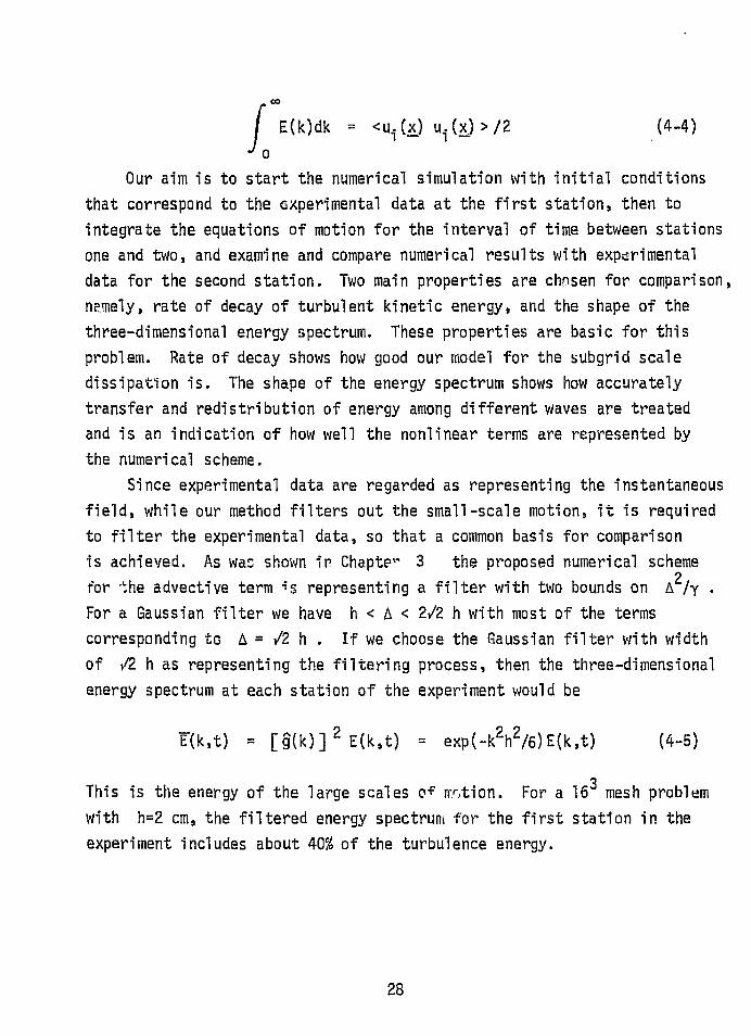
E(k)dk = <ui (x) u i (x .) > /2 (4-4)1 0

Our aim is to start the numerical simulation with initial conditions

that correspond to the experimental data at the first station, then to

integrate the equations of motion for the interval of time between stations

one and two, and examine and compare numerical results with experimental

data for the second station. Two main properties are chosen for comparison,

-J1 np.mely, rate of decay of turbulent kinetic energy, and the shape of the

three-dimensional energy spectrum. These properties are basic for this

problem. Rate of decay shows how good our model for the subgrid scale

dissipation is. The shape of the energy spectrum shows how accurately

transfer and redistribution of energy among different waves are treated

and is an indication of how well the nonlinear terms are represented by

the numerical scheme.

Since experimental data are regarded as representing the instantaneous

field, while our method filters out the small-scale motion, it is required

to filter the experimental data, so that a common basis for comparison

is achieved. As wa: shown jlr Chapter 3 the proposed numerical scheme

for -.-he advective term as representing a filter with two bounds on A2/Y .

For a Gaussian filter we have h < A < 2,/2 h with most of the terms

corresponding to A = ►/2 h . If we choose the Gaussian filter with width

of ,/2 h as representing the filtering process, then the three-dimensional

energy spectrum at each station of the experiment would be

M,t) = [ g(k)] 2 E(k,t) = exp(-k2h2/6)E(k,t) (4-5)

This is the energy of the large scales of mr tion. For a 163 mesh problem

with h=2 cm, the filtered energy spectrun: for the first station in the

experiment includes about 40% of the turbulence energy.

28

C. The Initial Velocity Field

T sle Fourier transform of an isotropic turbulence field of an incom-

pressible fluid should satisfy at least four requirements:

1. incompressibility

k i ca i (k^ = 0 (4-6)

2. real field[5i(7_k)

isotropy

<ui(k) ui (k)> - 0 Vi (4-8)

4. given energy spectrum

6 i (j) ut (k) - E(k)/27rk 2 (4-9) -

i .u.

In a numerical simulation, a modification should be made in Eq. (4-6) f.

to account for the representation of derivatives by finite differences.

In order to arrive at this modification in a simple way, consider the

one-dimensioi:al case. The finite-difference analog to the divergence

operator a/ax , which is used in the present work, is (D_) x where

(D- ) x u - (ui_Fji-1}/h(4-10)

The Fourier transforms of these operators are

a/ax T 3 .i. kX (4-11) f

(D_)x OFT^ [(l-COS 2" ) + i sinLm ^ /h (4-12)

where N is the number of mesh points in the discrete case, and m=kx/27r.

The Fourier operator associated with a continuous derivative is a pure

imaginary number, while in the discrete case it is a complex number, which

depends on the finite-difference scheme used. Therefore, the finite-

difference form of the incompressibility condition should be modified to

29

F

4

11

k3 (k) 5 i (k) = 0 (4-13)

where k!1

a complex vector field dependent on the finite-difference

divergence operator Di . This assures the numerical divergenceless

lk^!

condition in real space,

Diui(x) = 0 (4-14)

A method of generating a field which satisfies Egs.(4-7), (4-8),

(4-9), and (4-13) is described in detail in Appendix B. The generated

field is periodic in space, since a spectral method is used to generate it.

D. Results and Discussion

In Figs. 4-1 and 4-2 numerical simulation of decay of turbulent

energy and three-dimensional energy spectra are compared to experiment

for the case of isotropic turbulence with mean velocity of U O = 103

cm/sec behind a grid of bars of diameter M = 5.48 cm. The best fit

to the experiment was obtained with model constant c = 0.24 and

numerical constant a = 1/3 .

Figures 4-3 and 4-4 show the dependence of energy decay and energy

spectrum on the numerical constant a . While energy decay differs only

slightly for different values of a , the energy spectrum exhibits ani

irregular distribution in the a = 1 case, where energy piles up in the

region of high wave—numbers. This case is the staggered-mesh scheme used

by Harlow and Welch (1965), Deardorff (1970), and others. The proposed

scheme with a = 1/3 shows a more regular behavior, which suggests that

the Leonard term, which is included implicitly in this scheme, has an

important effect on the correct transfer and distribution of energy, and

should be included in the numerical scheme for proper simulation, especially

in problems in which the energy is spread over a wide range of wave—numbers.

This conclusion agrees with that of kwak, et al. (1975). It is interesting

to note that the staggered-mesh scheme with a = 1 contains implicitly

part of the Leonard term, as can be seen from Eqs. (3-26) and (3-27), and

4 was included in the past in simulations which used this scheme.

30

9

Sensitivity to ;he model constant is shown in Figs. 4-5 and 4-u.

The effect of changing c acts mostly on the high wave-number region.

The chosen value of c = 0.24 is 10% higher than Lilly's theoretical

estimate of c = 0.22 (Lilly, 1966) and more than twice the value used

by Deardorff in the channel simulation; he ran cases with c = 0.06 to 0.17

and chose c = 0.1 to be a representative value (Deardorff, 1970). Later,

in aa er devoted entirely to the problem of the magnitude of c'P p Y p g

(Deardorff, 1971), the author suggested that the large difference between

his numerical estimates and the value given by Lilly is due to the large-

scale valocity shear presented in his flow. Kwak, et al. (1975) have

found this constant to be c= .41.

Figure 4-7 shows the skewness defined by

7

S = <a3u/ax 3> / <@25/ax2 > /2 (4-15)

for different values of a . This function, which starts practically from

zero, reaches a maximum value and then declines monotonically. The maximum

value for S is in the range based on theoretical estimates (Batchelor,

1953, p. 172). However, 7 depends on the high wave-number part of the

spectrum and our result cannot be fairly compared with experiment.

In this chapter a numerical simulation of isotropic turbulence has

been shown to be feasible and to give acceptable results. Computation

time for a 163 mesh-point problem is about two minutes on the CDC 7600

computer. In the following chapters we shall use this method with constants

c = 0.24 and a = 1/3 to simulate homogeneous turbulence in the presence

of shear and system rotation.

31i'

20

4

2

In0XN 10t^

NO 8

6

w

100

80

163 MESH POINTS, h= 2 cm

FILTER: GAUSSIAN,A = -^'2- h60

MODEL CONSTANT: c = 0.24

NUMERICAL CONSTANT: Q= 1/340

0 COMPUTATIONAL

-- EXPERIMENT, COMTE-w BELLOT, CORRSIN (1971)

FILTERED EXPERIMENT

1L10

20 40 60 80 100

200tUp/M-3.5

Fig. 4-1. Rate of energy decay of isotropic turbulence,

4

32

loo

NlaV

10Ev

Iw

10

I

.j

}

iE:.

c.

7'

1000

i

IP

I.L

.8

cvl-%

INcr

L--j.I- - il 0

1000

100

MODEL CONSTANT: c=0.24

tuo /M =98

a= 1/3

a=1

Nipvin

EU

Iw

10

I.1

1 10

k cm-1

Fig. -4-4. Dependence of energy spectrum on numericalconstant.

r.a

35

in0X

N to[7

NOa

ev - W.i

r

100

1*

4

NUMERICAL CONSTANT: a=1/3

FILTERED EXPERIMENT

q COMPUTATIONAL

]I-10

100tUa/M-3.5

l oco

E^E v•M

!f3EIw

10

NUMERICAL CONSTANT a= 1/3

--- FILTERED EXPERIMENT

4

a

f;.

Fig.

1 000

-.4

-.3

S

-.2

Wco

—.5

MODE. CONSTANT c=0.24—_. is

0

50 100 150

200tUp/M-3.5

Fig. 4-7. Skewness for different numerical constants.

e

^CHAPTER 5

HOMOGENEOUS TURBULENT SHEAR FLOWY

A. General Description

Most natural and technological flows are shear flows. In shear

flows most of the energy is contained in the mean (time-averaged) velocity

field. When the flow is turbulent, there is a coupling between the mean

velocity and the turbulent fluctuations, and the flow characteristics are

determined largely by this interaction. In contrast to an isotropic

turbulent field with zero mean flow, in which turbulence levels are reduced

by dissipation, as was shown in Chapter 4, turbulence levels in shear

flows can be maintained or even increased by an energy-transfer mechanism

which subtracts energy from mean flow and feeds it into the turbulence

in preferred directions. This effect tends to make turbulence anisotropic.

Another characteristic of shear flows is the growth of length scales in

the direction of shear.

The simplest turbulent shear flow is the spatially homogeneous flow.

Numerical results will be compared with two experiments. The first ex-

periment is due to Champagne, Harris, and Corrsin (1970) (referred to later

as CHC flow) and the second is due to Harris (1974). Both experiments were

conducted in a wind tunnel. The shear flow was generated by a row of

parallel, equal-width channels having adjustable internal resistances.

A schematic sketch of the mean flow is shown in Fig. 5-1. In the first

experiment, measurements were taken between the nondimensional lengths

x/H = 8.5 and x/H = 10.5 , where x is the downstream coordinate, and

H is the height of the tunnel (H = 1 ft). The mean velocity gradient

was r = 12.9 sec -1 with a tunnel centerline speed of 40.7 ft/sec.

This setup was limited in performance and left only two feet for ex-

perimentation. In the second experiment the same setup was used, but

the mean velocity gradient has been increased to 44 sec -1 . If data are

referred to a dimensionless stretched coordinate x = (x/U c ) r , the

• high- and low-shear experiments appear as a continuation of each other.

Thus, the high-shear case can be regarded as low-shear data extended to

distance x/H = 35.

39

The purpose of these experiments was to confirm previous hypotheses 1

made by Corrsin (1963) concerning development of anisotropy with downstream

distances, which implies asymptotic nonstationarity of the flow in a

frame of reference convected with the mean flow. Another characteristic

that was found in the experiments was a growth in length scales in the

mean flow direction. The data will be presented when needed for comparison

with calculation.

In the numerical simulation we will try to assess these properties..., a

In addition, the pressure-strain correlation tensor T i p will be computed.

The pressure-strain term is responsible for the intercomponent energy

transfer. According to Rotta 0951,1962), it destroys shear stresses,

thus helps in redistribution of turbulence among the differon t components.

Numerical results will be compared to Rotta`s estimates.

B. Mathematical Formulation

The mathematical representation of a spatially homogeneous turbulent

shear flow is given by

<U > xz r ry + U (5-1)

<V> = 0 (5-2)

<W> = 0 (5-3)

<P> = 0 (5-4)

where U,V,W,P are instantaneous velocity components and pressure, which

include the mean flow, T is the mean velocity gradient, < > U are

averages over planes defined by ij coordinates, and < > are

averages over the entire space.

It is advantageous to change coordinates to a convective frame

traveling in the x direction with centerline velocity U . The mean

field in this frame is shown in Fig. 5-2. Let u,v,w, and p be the

obtain the equations for the turbulence, we subtract the mean flow out

by the following transformation:

u = U - y (5-5}

V - V (5-6)

Ig - W (5-7)r^

P = P (5-8)

Substitution of these definitions in the Havier-Stokes equations for

U,V,W,P (molecular viscosity is neglected) gives

f

at p ^ axj C(u+ry)uj

- ra (yu ) (5-9)

a - p ay - ax (vuj) - r 2x (yv) (5-10}

@w=

Tt-

1 ^ -

—P ax-j)(wu -r a`x (yw) (5-I I }

2

6xi axi = ..axi ax@X(ui uj } - 2I' ax ax(yuj } (5 -12)

In order to maintain these equations in a conservative form, no further

simplifications should be made by means of the continuity equation.

f

--

P x. ax. - ax. ax. (uiu32r ax ax. (Y^ (5-16)

i i i J J

If we set u u + u' and lump all subgrid components into the term

ax. ^ij we obtain) J^au _ a a

C(U+ry)u•a - r a (yu) + a

(5-17)'

at - - ax - axi ax axi xi

a - " ay ` ax. (vu^) r ax (yv) + ax . "yj ( 5-15}

a aF

at - az - ax. (wu^} - r xaxi

(Y) Tz;(5-19)

J

a- p- a (^a } - zr a a (yu } + a aY

axi axi axi axi i ax axj axi axj

(5-20)

All functionals of the form a/axi (yu) are treated numerically in the

same manner as the advective term a/axi (ui u.) , thus capturing implicitly

the Leonard tern that arises whenever a product of quantities is averaged.

iJ is assumed to be proportional to the rate-of-strain tensor of the

filtered turbulence components:

au auj )—j- (

5 -21 )^i^ = K axi + axi

K is given by Eq. (2-14), and we choose the model constant to be c 0.24,

as for the isotropic case (Chapter 4 } s on the assumption that the sub-

grid scales are nearly isotropic even in the presence of mean shear. It

should be noted that TiJ

now contains terms of the type iiiy i.e.,

averages containing the product of the subgrid scale turbulence and the

mean flow. These represent interactions of the mean flow with the subgrid

E! scale turbulence to produce resolvable scale f1wrttiati ons . Little isi

lF f

42

,wi1_.' '_

known about these terms or their effects, and in using the same value of

c as in the isotropic case we are tacitly assuming that they are

negligible. This point deserves further investigation but will not be

pursued here.

a. Boundary conditions

Since Eqs. (5-17) to (5-20) contain turbulence components only, and

^.^

we assume that the computational domain is sufficiently large compared

ko the characteristic length scales of the flow, we shall assume u i , p

to be periodic with respect to the computational domain. Although

convenient for numerical implementation, this assumption has some limita-

tions, in particular in shear flows. As we shall see, there is a growth

of length scales in the direction of mean shear. As time goes on, these

scales become comparable in size to the computational region, and periodicity

assumption is questionable. In the present simulation we start with a

jfield with a/H = 0.1, where X is the Taylor microscale, and H is

the length of the computational domain. Computation is terminated when

+

this ratio becomes - 0.2 . For longer simulations one must increase the

computational box, at least in the shear direction, if periodic conditions

are to be retained.

b. Initial conditions

The initial turbulence velocity field is chosen to be isotropic,

with identical energy distribution to that of the case described in

Chapter 4. The turbulence level is adjusted to <5i2> 1/2/Uc ru 0.022

which is approximately the initial value reported in the CHC experiment.

C. Computational time steps

The time steps are chosen to give a Courant number of NC = 0.25 with

respect to the mesh size h and the largest mean velocity Umax presented

in the flow field. For Umax = U

o/2 = 6.45 ft/sec and h = 6.25 x 10 -2 ft,

we find that At = 0.25 h/Umax - 2.422 x 10-3 sec. Using the Taylor

hypothesis for the convective velocity Uc = 40.7 ft/sec, the following

relation holds:

x

4

43

i

r

10 time steps -E--•-- ' 1 ft

These quantities will be used throughout the numerical simulation of the

present and the following chapter.

C. Results and Discussion

a. Comparison with experiments

Figures 5-3 and 5-4 compare numerical simulation to experiments.

The first figure compares the turbulent levels in different directions.

As in the experiment, the v and w components, which are perpendicular

to the shear direction, decay monotonically with distance, while the level

of U , the component in the shear direction, behaves differently. At

first it decays, then it levels off and starts to grow. The growth of

E in the CHC experiment is not clear enough, but it is shown clearly

in the extended experiment made by Harris. Numerical results confirm

the experimental evidence which shows that in the presence of mean shear,

energy is extracted from the mean shear and fed into preferred turbulence

components. This growth makes the flow nonstationary in a reference

frame convected with the centerline velocity U .

Bate that the computed results show faster growth than the experi-

mental results. To bring the computations into agreement with experiment

would require increasing the subgrid scale constant c which is incon-

sistent with what Deardorff (1970) and Schumann (1973) found. Furthermore,

the neglected interaction between the mean flow and the subgrid scale

fluctuations should be a production term and would tend to reduce the

subgrid scale constant. Thus, although the computed trends agree with

experiment, the results do differ quantitatively and the most obvious

possible causes would change the results in the wrong direction. The

remaining possibility, i.e., that the difference is due to improper

initial conditions, is also not likely to be correct as an isotropic

initial condition should yield the smallest growth rate for a given

turbulence level.

+i

44

A

a

The second figure compares the Reynolds shear stress - < W>As we shall see later, this shear stress acts together with the mean

shear to create a production term for the turbulence in the x direction.

This term is important also in two-dimensional turbulence modeling. Asis shown, computed results agree quite well with experiment. These com-parisons, although limited, bring us to the conclusion that the numerical

simulation properly represents the main features of an actual shear flow.

b. Additional numerical results

In Figs. 5-5 to 5-11 additional information is extracted from the

numerical simulation. Some of this information is either difficult orimpossible to obtain experimentally. Examples in the first category are

spatial correlations and length scales, and in the second catego ry ars

pressure-strain correlations and the "return to isotropy" simulation.

This information extends considerably the existing data set for shear

flows and can be of help in two-dimensional turbulence modeling. A

detailed description of these data follow.

Figure 5-5 shows the development of total turbulent kinetic energy

ui ui with time (or distance). Since the initial field is isotropic,

energy starts to decay at an equivalent rate as in the case of isotropic

turbulence with zero mean flow (Chapter 4). As anisotropy develops,

enough energy is extracted from the mean flow to compensate for dissipation,

and to allow the net energy to increase. There is no reason to believe

that the growth will not remain indefinitely; the steady mean field

implies that it is being pumped in such a way as to maintain its energy.

Figure 5-6 shows the development of turbulent levels in each direction.

Figure 5-7 :Shows the three components of shear stress -< u i uj >

(normalized on the RMS values of ui and uj ) . Ideally, initial conditions

for these terms should be zero, if the field is truly isotropic. Prac-

tically, it is difficult to achieve this requirement in a 16 3 problem.

Nevertheless, the flow adjusts itself after a short period (about thirty

steps) and the terms - < uw > and - < vw > are reduced to zero (wi thin

an error band of 0.01). The value of -< U> , on the other hand, growsto an approximate value of 0.5.

45

R

%k

Figure 5-8 shows the development of length scales aj in each

direction. The length scale in the shear direction grows considerably,

while in the other directions there is not a significant change. Although

experimental data for the length scales exist in the CHIC experiment,

comparison can be made qualitatively only. The reason is the large

difference in the initial length scales of the experiment ( X u .016 ft)

and the numerical simulation (l n,.10 ft). This difference comes Mainly

from the fact that in the numerical simulation we are using filtered

rather than instantaneous quantities, and there is a considerable difference

between (au/Ox) 2 and (8u/ax) 2 which occur in the definitions of

A and a , respectively.

The explanation for the observed behavior of the turbulence quantities

and length scales that we prefer is that small nearly circular, eddies

with their vorticity in the z direction combine to form elongated eddies

with their major axes in the x direction. Such a process, similar to

the vortex-pairing process put forward by the USC group (Winant and

Browand, 1979) would lead to an increase in < u 2 > , a decrease in < v2 >,

an increase in ax , and a constant ay . It will also decrease < z >1

which was observed but is not shown in the figures.

Figure 5-9 shows nine components of spatial correlations. The most

significant change occurs in the R 11 (x,0,0) component. The reason for

that is the growth of length scales in the x direction which makes the

flow correlated over larger distances. It should be noted that the least

changes occure in the z direction, which means that most of the inter-

action takes place in the (x-y) directions.

Figure 5-10 shows the development of the pressure-strain correlation

tensor Tij , where

_ @6 i auk

Tij - < p fix. ^ ax } > (5-22)

C

In an isotropic field of turbulence these terms should be identically

zero. As can be seen, the initial values, as with the stresses _< ui u j >

are not zero, and a period of adjustment should be allowed before any

conclusion can be drawn from the simulation. In the present case we

4

46

shall refer to data at time step L = 100, where the Tii show regular

behavior, and the length scales have not increased so much as to invalidate

the periodic boundary conditions used in this simulation. More details on

Tip will be given later in this section.

Figure 5-11 shows a "return to isotropy" simulation from a sheared

state. As the mean shear is turned off, the flow returns to isotropy

in a peculiar way. When the amount of anisotropy is large, there is a

transfer of energy between u and v which causes initially an increase

in the v component. When the anisotropy diminishes, dissipation effects

take over and all three components decrease toward isotropy. No such

effect is observed in the w component, which suggests that most of the

interaction and energy exchange is two-dimensional. This can be explined

physically by the rotation of the elongated eddies that were formed by

pairing. (In the absence of strain an elongated vortex will rotate.)

C. Pressure-strain correlation Tii

The energy and stress balance equations for a homogeneous shear flow

are given (Hinze, 1959, p. 252) by

at `2 u2 > - < -uv> r + Til + Dsgs (5-23)

at < 1v2 > + T22 + Dsgs

(5-24)

at < 7 w2 > = + T33 + Dsgs

(5-25)

at < -uv > w < `12 > r - T12 + Dsgs

(5-26)

Dsgs stands for a subgrid dissipation term which will not be specified

explicitly here. T i , is defined in Eq. (5-22).

Initially, when the flow is nearly isotropic, Tip is identically

zero. As time elapses, the term <^ 2>r in Eq. (5-26), which is positive

definite, causes a positive increase in the stress term <-uv> . This,

in turn, increases the turbulence level of <5 2> in Eq. (5-23), thus making

471

k

y

a:::.

the flow anisotropic. When the field is anisotropic, the terms T ij are

no longer zero. The values of Tij grow in a way which tends to equalize

the velocity levels and reduce the shear stresses. Qualitatively, the

val ues of Tij should be as follows:

T11 < 0 , T22 > 0 , T33 > 0 , T12 > 0 (5-27)

This is indeed what we find in Fig. 5-10.

Because of the importance of the term Tij , and the extreme difficulty

of measuring it, it has long been a subject of model estimation. One of

the simplest and most popular models is Rotta's estimate (1951, 1952),

where he assumed that the pressure-strain correlation tensor is proportional

to the amount of anisotropy presented in the flow:

Tij - -A D bij (5-28)

where D is the isotropic dissipation given by

-D = at (q2/ 2 ) (5-29)

and bu is the anisotropy tensor def-ined by

bij = ( Rij - q2 6 i j/3)/q2 (5-30)

(R ii= <ui uj > , q2 = Rii )

This model has been checked with data obtained from the "return to

isotropy" simulation (Fig. 5-11). The results (for L = 280) are as follows:

a. component T17 gives a constant A = 2.3

b. component T22 gives a constant A = 3.8

c. component T33 gives a constant A = 1.4

These results agree with estimates made by Norris and Reynolds

(Reynolds, 1975). They recommend a value of A = 5/2 which is the

average value of what we find for the separate components of Tij.

48

i

Fig. 5-1. Schematic sketch of the homogeneous turbulentshear flow.

49

^Uo/2

<u >xx = rY

Y

x

Fig. 5 -2. Mean velocity in a convective frame.

50 i

^a

[o.

s.

6.

4.

P%

2.0

NIQ

X

^ I.0

A .8N•-I^V .6

.4

U

WO

00O 0

o a o oQQEl A

a

V ^L7[3Cl

07d70 COMPUTATIONAL

2 EXPERIMENT, CHAMPAGNE et a[. (1970)

---^^ EXPERIMENT, HARRIS (1974)

2 4 6 8 10 20 40 60x/H

Fig. 5-3. Turbulence levels in homogeneous shear flow,comparison with experiment.

51

1.0

C-A

I>vA

04 .5I=v

AI>1:3

vI

01I

C)

3 5 7 9 11 13 15 17

x/H

Fig. 5-4. Shear stress in homogeneous shear flow,comparison with experiment.

52

^O

X

j ':

.04

.03

NA .U2

N^17V

.01

,j,-!1

0 20 40 60 80 100 120 140

NUMBER OF TIME STEPS

Fig. 5-6. Development of turbulence levels inhomogeneous shear flow.

54

1.0

.5

1

AN•-+

v cA

N•-I^

V^

A1:

VI

-1 L0

4

20 40 60 80 100 120 140

NUMBER OF TIME STEPS

I

d

Fig. 5-7. Development of shear stresses in homogeneousshear flaw.

55

.3

.2

xi/H

0 20 40 60 s0 10(NUMBER OF TIME STEPS

i

Fig. 5-8. Development of length scales in homogeneous -shear flow.

56

€ f

^ • ^ a 6 ^ s

0

C

cn4I

C

RI 1 (x,0,0) -, RI I (01 y, 0) `^ R I 1 (0, 0, x)

♦` IR22(x,O,O) ♦ R22(0,Y,0) R22(0101z)

♦` R33 (X, 0, 0) R33 (0, Y, 0) R33 (0, 0, Z)

Lw140

L=20

0

2 4 6 R z Iq '} a a

r/h

Fig. 5-9. Spatial correlations in homogeneous shear f ► cw.

12040 60 aO 100

NUMBER OF TIME STEPS

Fig. 5-10. Development of pressure-strain correlationsin homogeneous shear flow.

-4Q

-2

-3

4

3

2

140

T1j

0

58

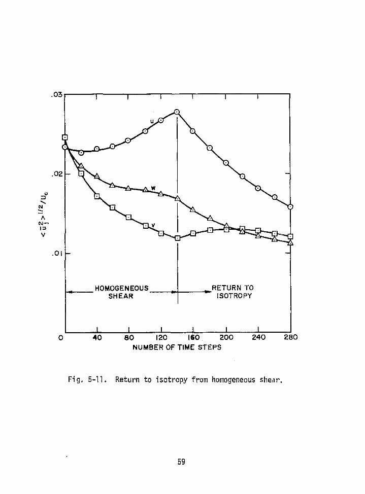
.03

.02

U

N

AN..-.i:3V

01

IL

ft

0 40 80 120 160 200 240 280NUMBER OF TIME STEPS

Fig. 5-11. Return to isotropy from homogeneous sheer.

59

CHAPTER 6

HOMOGENEOUS TURBULENT SHEAR FLOW WITH SYSTEM ROTATION

A. General Description

The third problem to be simulated adds one more parameter to the

flow field. Homogeneous turbulent shear flow is examined in the presence

of system rotation. This problem is of interest in two important fields.;

The first one is atmospheric turbulence where the flow field is in a

rotating frame of the earth, and the second is the internal flow of turbo-

machines. Rotation has an effect on the stability of turbulence. It

has been shown by experiments (Halleen and Johnston, 1967) that, depending

on the magnitude and direction of rotation, either augmentation or sup-

pression of turbulence intensities results. Johnston (1974) investigated

the effects of rotation on boundary layers in turbomachine rotors and =

proposed a relation for the mixing-length ratio Q/Qo (used in two-

dimensional turbulence modeling) which is based on the local gradient

Richardson number defined by

Ri W29(r 2S2

(6-1)r

in the form

Q/to = 1 - Ri (6-2)

where Q is defined by

Q - <U>> 1/2 /r (6-3)

Based on experiments, S was found to be in the range of 2 to 6.

Since our simulation represents a small region of the flow field

away from solid boundaries or other interfaces, we do not claim that this

simulation represents a real flow such as exhibited in an interior of a

turbomachine; therefore, comparison with available experiments should be >>

made carefully, if at all, at this stage. On the other hand, the experi-

ments are involved and results are affected by effects other than rotation,

as can be seen from the scattered data of the experiments (Fig. 6-6),

60

while the numerical simulation is "clean" in the sense that we are testing

the eXclusive effect of rotation on the flow.

In the following, numerical results will be given for different

Ri numbers and will be compared to experiE-nent, and a simple explanation

will be given for the stabilizing effect of rotation on the turbulence.

B. Mathematical Formulation

The equations of motion relative to a frame which is rotating in

a constant angular velocity 9 are given (Batchelor 1967, p. 144) by

aufU -vU = - Pat VP-20xU -0x (aU) (6-4)

V - U = a

(6 -5)

The term -2QxU is the Coriolis force, which is perpendicular to both

U and 0 , and -Qx (a>U) is a centrifugal force, which can be written

also as

- 1 v (UxX) 2

(6-6)

This term can be added to the pressure term -1/p 0 P to form a generalized

pressure P*:

P* = P + z p (a x) 2 (6-7)

In Cartesian tensor notation the equations of motion read

au i {- - ..

at Dxa

i (Ui `^,j} P @Xi* 2s i;k s^a Uk (6-8)

a1i

axi r C(6-9)

Let Q = (a,O,n), and the velocity field be defi ned as

61

i 1

< U > Xz = r y (6-10)

< V > = 0 (6-11)

<W> = 0 (6-12)

We define also a mean pressure

< P > Xz 7- - p 92ry2 (6-13)

To obtain the equations of turbulence, we subtract the mean values from

the instantaneous field:

u = U -ry (6-14)

v V (6-15)

w = W (6-16)

P = P* + PQr y2 (6-17)

Substitution of these definitions in Navier-Stokes equations for U,V,W,P*Y

Eqs. (6-8) and (6-9), gives

at = - p a ' ax C(u+ry ) uj l - r ax (yu) + 20v (6-18)

av = - p r ax e (vuj) - r ax - 2Qu (6-19)

awat ` - p az - axj (wuj) - r a (yw) (6..20)

2

axi a i - axi ax • (ui uj ) - 2r ax ax. (yuj ) + 2AV -

ay/(6-21,)

J J

Following the same procedure of averaging described in Chapter 5, Eqs.

(5-13) to (5-20), we get the conservative form of the filtered equations

of motion relative to a rotating frame.

^I

I

62

a -axj 1( ax- r a (yu) ax j Txj + 2nv ( 6-22)4

0

av` a (vu } - r a (A + a T - 2r (6-23)at - ax - axj j aX axj A

^.

az - ax { luj ) - ^' x {yw} a-

axa Tzj (6-24)

ax•ax• - ax• ax. (u i uj ) -r ax ax. (yuj} + 2S2 ax ay} r ax• aaj Tij

7 3 'L ^ / 7a a

(6-25)

Again, we use periodic conditions for the turbulent components u i , p .

Initial conditions are isotropic with the same energy spectrum as for

the case given in Chapter 5.

C . Res ul is

Four different values for 0 were used in the simulation: Y

n = ^ -1.33, -.591, .727, 3.22 -

which correspond to gradient Richardson numbers:

Ri = .25, .1 , -.1, -.25

The mean velocity gradient was kept as in the case of n = 0 in Chapter

5, r = 12.9 Sec -1 . Figures 6-1 to 6-5 show the dependence of the total

turbulent energy < 5 ig i > , the shear stress -< uv> , and the turbulencelevels < u?>

112 on Ri As can be seen, turbulent intensities and

shear stresses are higher for larger rotations (or smaller Ri numbers)

and vice versa, which means that rotation either stabilizes or destabilizes

the turbulent field, depending on the magnitude and direction of 9 .With regard to the turbulence levels, the most profound change occurs in

the v component, where rotation changes its behavior entirely from a

decaying triode for Ri = .25 to a rapidly growing mode for Ri = -.25 .

63

I

^ a

It is interesting to note that for Ri = -.25 , turbulence levels of u

and v are almost identical (a simple explanation will be given later

in this chapter).

Figure 6-6 shows the dependence of mixing--length ratio on the local

gradient Richardson number, as was evaluated from experiments (Johnston,

1974). As was mentioned before, this experiment is quite complicated

and data are scattered, which makes any interpretation difficult, at best.

Contrary to the experiment, which is conducted in stead--state conditions,

our simulation exhibits nonstationarity. Nevertheless, if we analyze

data from time step L = 100, at which time the flow has developed

(but not too much to invalidate the periodic conditions), we find that

a ti 1.7 which is in the lower range of experimental results (Fig. 6-6).In an attempt to obtain simple correlations, we have plotted < U >

and < 0 >1/2 (which is proportional to the mixing length)versus both 0

and Ri . The best fit was obtained with <5V >1/2 versus Ri and is

shown in Fig. 6-7. We find

< U > 1/2 ti C 1 - C2 Ri (6-26)

where C 1 ti .5 and C 2 ti .04t-2D. Interpretation of Results

Simple shearing motion can be viewed as a superposition of a pure

straining motion and a rigid rotation. When simple shear and rigid rota-

tion are applied together, there is a value of rotation which cancels

the rotational part of the shear and thus reduces the flow to a pure

strain, the principal axes of which are at 45° to the (x y) axes. The

case of simple shearing motion in a rotating frame is similar. Let us

write Eq. (6-8) in the form

at + uj (Ii j +R i j ) + uj p i j = I ax*

(6-27)

where

aui1 i j 2-l a. UI.`3 - I ax. r ax. )

(6"28)1

,a

64 j

`f

J

p i j = 2 E ikj 52k (6-30)

For simple shear with M/ay = r and 2k _ (0,012) we have in two

dimensions

< < 0 r/2

ij(6-31)

( r/2 0

1 0 r/2

(6-32)

r/2 0

0 -252

pij = (6-33)

252 0 )

It is easy to see that if r/2 = 252 , then G_ij

pij and the motion

reduces to pure strain with principal axes at 45°.

The general form of the turbulent shear stress tensor for pure

strain in the principal axes (two dimensions) is given by

<u2 > 0

(6-34)0 < v2 >

If we rotate this tensor 45 0 , we obtain

7 <u2*>+<v2>

<u 2 > _ <v2> (6.35)I <U2>_<^2> <u2 > + <v2>

with the result that the terms on the diagonal are equal. If we examine

the case of pure shear in a rotating frame with r/2 = 20 or a = 3.22

(Ri = -.25), we find that within computational accuracy the diagonal

elements of < -Ui uj > are equal , or < 5

2 > 1/2 = < v2 > 1/2 , as can be seen

from Figs. 6-3 and 6-4.65

t

This view also leads to a simple picture of turbulence production.

If we focus strictly on the production terms, then the three most important

i equations for the turbulent velocities may be written:

d 2dt > - _2<62>3 l 11 - 2< u-v >J12 - 2 < uv A l2 (6-36)

2d dt > - -2 < v2 >^22 - 2 < uv >j l2 + 2 < uv >R 72 (6-37)

d N> - _<N>(317 + 22 ) - ( <u2 >+<G 2 > )^72 - ( <v2 >_<u2> }R72

(6-38)

where R 2 =0 2 p7 2 and we have noted that 312 j21 ' ^` 7 2 - -/P21

t

Without loss of generality we can choose the principal axes to be along

the coordinate r,irections so that

_tJ 12 - 0 , 2 ^11 = -2 ^ 22 = s , 21R 12 2 r (6-39)

and Eqs. (6-36) to (6-38) reduce to

d<E2 >

= s< 52 > - r <GG> (6-48)

dt

d< 2 > -- -s<v 2 > + r<uv> (6-41)

d<dtv> = -^r( <v2 > - <u2 >) / 2 (6-42)

The kinetic energy obeys the equation

at < 52 > + < G 2 >) = s ( < 5 2 > - < v2 >) (6-43)

`

so that there is no production of turbulent Kinetic energy if the tur-

bulence is isotropic. If, however, < u 2 > > < v2 > , there will be

growth caused by the fact that < 5 2 > grows faster than < i2 > decays.

66

8

Thus, if the turbulence is anisotropic, there will be production, and the s

production is in such a direction as to increase both the energy and the

anisotropy.

It is interesting to note the effect of rotation on production.

Equations (6-40) to (6-42) are linear ordinary differential equations in

<u2> , < v2> , and < 5v> and thus have exponential solutions. Seekingii solutions of the form eat we find r

a = 0 f s2 - r2(6-44)

Thus, we see that the greatest production results when r 0 i.e.,

for pure strain (corresponding to Ri = -.25). Any rotation inhibits the

production and, in fact, for r > s there is no production at all.

When r = s , the growth is algebraic.

Physically, rotation mixes the components, i.e., it transfers some

of the a component to the v component. In so doing, it reduces the

anisotropy and, indirectly, inhibits the production of turbulent kinetic

energy.

67

'ox

cu^ 1

a

vc s

1

2 1 l-

Ri = —0.25/ f

/J

' O

^.25

DECAY OF ISOTROPICTURBULENCE ^.t

Ri = -0.25 1^^r-0.10

ter " 0.10

0.25

nnvn

r^ .5

nvt

1.0

t:.

a.

r w

.03

.02

Ri = -0.25

-0.10

0v 0

010

0.25

N

nNI}V

.01

I

k

0

Ri= -0.25

-0.10

0

O'lo /

0.25 ^

.02

03

01i

30

1/10

2.0

*t.v

3.O

00

00

E); 4 .<

=2

0 N 19=2

A

C

El 0 •

R=6 =4

1.0

Lu

.8

.6

1/10 .

4

.2

1 0 COMPUTATIONAL

0 -.10 -.20 -.30 0 .10 .20

Ri Ri

Fig. 6-6. Mixing length ratio versus gradient Richardsonnumber. Data from Johnston (1974).

1.2

1.0

Cli

A

V

-.30 -.20 -.10

Fig. 6-7. <N>1/2 versus gradient Richardson numberat various time steps.

JU t

74

CHAPTER 7

SUMMARY

A. Conclusions

Three-dimensional time-dependent numerical simulations of simple

turbulent flows using the filtered incompressible Navier-Stokes equations

with the simple formulation of Smagorinsky for the subgrid scale eddy

coefficient prove to give very reasonable results. Although the number

of degrees of freedom of 16 3 mesh points is limited, with respect to

resolution, it was shown that useful information can be extracted from

these simulations, which contain much of the physics of these flows.

Furthermore, the approach is convenient and reasonably economical with

regard to speed and capacity of available computers.

The proposed numerical scheme for the filtered advective term,

which contains a Leonard term implicitly, was shown to be important for

proper energy transfer down the wave-number scale and is recommended for

use in future investigations, in particular when long time integrations

are needeO and when the turbulent energy is spread over a wide range of

wave numbers (high Reynolds numbers).

The imposed periodic conditions for the turbulence, which have been

used in all of our examples, have advantages as well as disadvantages,

The advantages are twofold. First, the mathematical problem is well

posed on the boundaries, and does not introduce errors into the domain

of numerical integration. Second, periodic conditions allow the use of

rapid routines in the solution of the Poisson equation. The disadvantage

is that turbulent length scales must be kept small compared to the -;ompu-

tational dimension, and in problems where these scales grow s numerical

simulation cannot be carried out far long times without invalidating

this requirement.

B. Recommendations

Based on the experience gained in this work the following recommen-

dations are proposed for future work in this field:

75

1. Improvement of initial conditions to allow better

control on the statistics of the velocity and pressurer

fields such as stresses < ui uj > and pressure-

strain correlations Tip .

2. Extension of boundary conditions to allow other con-

ditions than periodic. For example, treatment of a

rotational-irrotational interface and a solid boundary. .

3. Extension of the computational region, at least in

important directions such as the shear direction in

a homogeneous shear problem, to allow longer integra-

tion periods. This will require the use of peripheral

equipment.

4. Simulation of other basic flows for which experimental

data exist such as vortex pairing and far field

solutions of jets and wakes.

This work is one of many efforts made in recent years the aim of

which is to explore the basic problems of turbulent flow simulations,

and it is believed that eventually it will bring about the solution of

actual problems on the engineering level.

76

N .

A

I

I

APPENDIX A

THE FILTERING OPERATOR AND ITS PROPERTIES

The filtered function f(x) is obtained as the convolution integral

of the function f(x^ with a filtering function g(x)

T(x) - g t f(x) - g(x-x') f(x') dx' (A-1)

all space

X. x are position vectors whose components in a Cartesian system are

X, y, z and x', y ` , z' respectively, and dx' is the volume element

dx' dy' dz' .

The only requirement on the filtering function g(x) is that it is -

Fourier transformable, which means that it should be square integrable.

Since

[g ( .?o # f(x) = i ki 9Q0 f( 0 (A-2) .and

ag(x)

ax i

# fW - i ki g W f(k) (A-3)

and also

The filtering function used in this work for averaging the

Navier-Stokes equations is the Gaussian filter defined by

1J2 3g(x)

^exp (-61x[ 2/A2 ) (A-7)

the Fourier transform of which is

nj. A

g (k) = exp(- q2 (k! 2J24) (A-8)

Other functions can be used as well. For example, the running mean

filter is defined by

1 I LI < box of sides Ag(x} _

A3 (A-9)

0 IxI > box of sides A

its Fourier transform is given by

3 sin (k 6/2)

g(^ _ 7rk ^/2

(A-10)

i = l i

This filter has been used by Deardorff (1970). For a detailed discussion

of the properties of these filters see Kwak,et al. (1975).

44

.i

i

Y^

M

1

78

-- -- -T

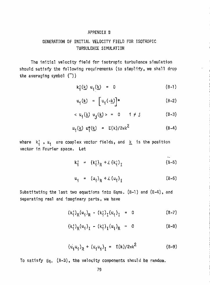
I APPENDIX B

GENERATION OF INITIAL VELOCITY FIELD FOR ISOTROPIC

TURBULENCE SIMULATION

The initial velocity field for isotropic turbulence simulationshould satisfy the following requirements (to simplify, we shall drop

the averaging symbol (—))

k! u l 0 (B-1)

ui Cui (B-2)

< u i (L) uj > 0 i j (B-3)

u i (k) ui E(k)/27Tk 2 (B-4)1

where k! , u are complex vector fields, and k is the posit-Ion

vector in Fourier space. Let

k! NOR +i M), (B-5)

u (B-6)i (ui)R (ui)I

Substituting the last two equations into Eqns. (B-1) and (B-4), and

separating real and imaginary parts, we have

(k!) R (ui ) R(k! ) I (u i ) l 0

(B-7)

(k i') R (u i ) I I(k!)

I (u i ) R 0(B-8)

(u:iui)R

(ui u i ) jE(k)/27rk2(B-9)

+

To satisfy Eq. (B-3), the velocity components should be random.

79

The required field is generated in two stages. First, two fields

iIui

2 ui are generated, with k^ real and equal to (k )R and (M) I ,respectively. Second, the fields are combined to give the required •

i field that satisfy Eqs. (B-1) to (B-4).

Let us assume for the moment that we have generated these two fields;

then: -

i

(k!) = o (B-10)4

til2i

i

e

Iui I ui W 2 u 2 ui -E (k)/2uk2 (B-12)

Let the desired field be a linear combination of the two fields

(u i } R - a I ( I u i ) R a2(2ui )R (B-13)

( u i }I = a3 ( l u i ) I a4 ( 2u i ) I (8-14)

If

Substitute Eqs. (B-13) and (B-14) into (B-7) to (B-9) and use Eqs.

'j (B-10) and (B-11) to get

a (k!) R ( 2u-) - a (k!) I ( u.} = 0 (8-15)2 R 3 z 1 I

al (ki) I ( l ui ) R - a4 (ki) R ( 2 u i ) I = 0 (B-lfi)

a2 ( u. u } 1 2a a (u, u } + a2 ( u. u.}1 1 i 1 i R l 2 l l 2 i 2 7 2 7 8

+ a2 (u• u) +2aa(u. u) +a2 ( u u) (B-17)3lZliT 341j2iI 42i 2iT

OP= E(k)/27rk2

4

80

{

In order to determine the field u i , we have to determine the

constants a l , a2 , a3 , a4 - This is done by solving the three algebraic

equations (B-15) to (B-17) in four unknowns (one is determined arbitrarily),

for every value of k i in the region k3 < 0 . The other half-space

k3 > 0 is obtained by condition (B-2), which makes u i (x) real.

V e two separate fields are generated as follows: Consider a

coordinate system in Wave-number space, as shown in Fig. B-1. For any

position vector k i , the vector k! is specified, k! depends on the

specific finite-difference scheme used for the divergence operator; for

example, see Eq. (4-12). Let u be a vector which lies in a plane P

perpendicular to Q , and which makes an angle ^ with a reference

to vector t which is the intersection of P and the plane formed by

k and 2,3 is chosen randomly in the range (0,27x) . u i u i is

chosen to be equal to E(k)/27rk 2 . Let rj be another random number

in the range (0,1) . Decompose u i u i into two parts such that

(u i uO R = n(u i u i ) (B-18)

( ui u i ) I = (1-n)( u i u i ) (B-19)

Then decompose (u i u i } /21/2

eand (uiui)I eu into their components

along the vectors e l ems,,, , e 3 according to the formulae

(ul ) R -(cos C cos ^ cos 8 + sin 9 sin e ) (u i u i ) 1/2 (B-20)

( u2 ) R = (-cos cos o sine + sin E cos a )( ui u i ) R/2 ( E -21}

( u 3 } R = (cos sin)(u i ui )/2 (B-22)

i (ul)I = -(cosh cosh core + sinE sine )(u l u i )T /2 (B-23)-

(u2)I

j11 q

= (-cosg cosh sine + s in p- cose)(ui ui ) /2 (B-24)

8l(^I E1{

-

^I

IF

(u3

) I (cos ^ sin )(u i ui ) 1/2(B-25)

This procedure is repeated twice for (M ) R and (k!)I . The sub-

routine INICON is a realization of this method.

i

ik

I

i

a

82

i

-1

Fig. B-i. Coordinate system for decomposition of u

83

z APPENDIX C

THE DISCRETE FOURIER TRANSFORM AND ITS

COMPUTATIONAL FORM

The truncated sum of a Fourier expansion up to wave number N/2

is given by

N/2-1f(n) = F(m) exp(27r i mn/N) n=0,...,N-1 (C-1) #E`

m=-N/2 a

The inverse of this transformation is given by

F(m) = N Jl f(n) exp(-27r.cnm/N) m=-N/2,...,N/2-1 (C-2)n-0

A more frequently used transform pair is given by the definition

N-1f(n) _ E F(m) exp(27r-i.mn/N) n=O,...,N-1 (C-3)

m=0

F(m) = N Fl f(n) exp(- 2Tryi. nm/N) m=O, ... ,N-1 (C-4)

n=O

which is used in most fast Fourier transform (FFT) algorithms.

Since exp is a periodic function in N , it is, in general,

immaterial whether one set is used or the other. Both will recover6

the original function after applying a transform followed by an inverse.

However, when discrete Fourier transforms are used to solve differential

equations, the first pair should be used, otherwise the method will pick

up an aliased solution which contains higher frequencies. Nevertheless,

it is not required to give up the existing FFT codes, because there is

a one to one correspondence between the two definitions.

Consider that f(n), n=O,...,N-1 is given. Then, according to

Eq. (C-2) we have

c

84

iIiI

I

-

^ -

F{m) _ ^1 f (n) exp(-27ri nm/N) m=-N/2,...,N/2-1 (C-5)

iN n=0 F `?

1N-1 m+n for -N/2 < m< 0

—yf (n)

N

- exp ( -2^r.i. nm' /N) m' --

n=0 m for 0 < m < N/2-1

m now varies from 0 to N-1 as in Eqn. (C-4), but the ordering of

F (m) has been changed. As an example, consider the case of N = 4 Let

f (n) = f(0) , f(1) , f(2), f (3)

The discrete Fourier transform of f(n) using Eqn. (C-2) givesi'

F(m) _ F(-2), F(-l), F(0)^ F(l)

while using Eqn. (C-4) the order of F(m) is changed to

F (m) _ F( 0 ), F ( l ),F (-2 ). F(-l)}

For a detailed description of the fast Fourier transform algorithms the

reader shoul d see Cochran, et a1 . (1967) .

x --

r 85,

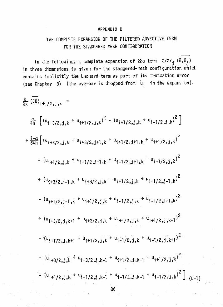
APPENDIX D

THE COMPLETE EXPANSION OF THE FILTERED ADVECTIVE TERM

FOR THE STAGGERED MESH CONFIGURATION

In the following, a complete expansion of the term D/ax J Ni5J}'

in three dimensions is given for the staggered-mesh configuration which

contains implicitly the Leonard term as part of its truncation error

(see Chapter 3) (the overbar is dropped from U i in the expansion).

8x (65)i+l/2,j9k -

a 2 2AFh [(Ui+3/2,j,k + u i

+1 /2,j, k) (u i+1/2,j ,k + ui-1 /2,j,k}

l-a 2+ 64h I

(ui+3/2, j ,k +

u i+3/2, j+l,k ui+l/2,j+l,k + ui+1 /2,J,k)

Y

2(u i +1/2, j , k + u i + 1

/2,J+l , k + u i-1/2,j+l ,k + ui-1 /2,J,k)a

2+ (u i+3/2,j-1,k + u i+3/2, j ,k + u i+1/2, j ,k + ui+1 /2,J -1,k)

_

2(u i+1/2,j-1,k + u i+1/2, j ,k + u i-l/2, j ,k + ui-l/2,j-1,k)

+ (u i+3/2, j ,k+l + u i+3/2, j ,k + ui+l/2, j ,k +

2ui+1 /2,j,k+l)

- (u i+1/2, j ,k+1 + U i+1 / 2 , j ,k

+u +^^i-1/2, j ,k.

)2i-1/2,j,k+1

+ (u i +3/2, j ,k + u i+3/2$ j , k -I + u i+1/2,j ,k-12

+ ui+l/2,3,k}

- ( ui +1 /2)J,k + ui+l/2, j ,k-1 + u i -1/2,j,k-1 + ui-1/2J,k)2D-^{ ).^86.:.#:.

DY

[(ui+1/2,j,k + ui+1/2,j+1,k )(v i+l,j+1/2,k + vi,j+1/2,k)

- (1li+1/2,j-1,k +

u i+1/ 2 , j , k) (vi +1,j-1/2,k i,J-1/2,k)I

+ 1-a [(141+3/2,j,k16W + ui+3/2,j+1 ,k + U i+1/2,j+1 , k + ui+1/2, j , k vi+1 ,j+1/2,k

- (ui+3/2, j -1,k + ui+3/2,j,k + ui+1/2,j,k + Ui +1/2,a-1,k)vi+1,j-1/2,k

+ (u i+1 /2,J, k + ui+1/2,j+l ,k + u i-1/2,j+l,k + ui-1/2,j,k)vi,j+1/2,k

(ui+1 /2,j-.l,k + ui+1/2,3, k + Ul-1/2,J,k + Ui-1/2,a-l,k)vi,j-1/2,k]

1-a++ +

ui+1 /2, j+1 ,k + u i+1 12,j , k+l + u i+1 /2, j+1 ,k+1)

' (vi+l , j +1/2,k + v i , j+1/ 2 , k + vi+l , j+1/2,k+1 + vi ,j+1/2,k+1)

(ui+1/2,j-1 ,' + u i+1/2, j ,1; + ui+1/2,j-1,k+l + Ui +1/2,j,k+l)

(v i+1,j -1 / 2 , k + vi, j -1/2,k + v i+1 , j -1 / 2 , k+1 + vi ,j-1/2,k+l)

+ (ui+1/2,j ,k-1 + ui+l /2,j+1,k-1 + u i+i/2, j ,k + ui+1/2,j+l ,k)

(vi+1,j+1/2,k-1 + vi,j+1/2,k-1 + vi+l,j+1/2,k + vi,j+1/2,k)

(ui+1/2,j-1,k-1 + ui+l/2,J,k-1 + ui+l/2j-1,k + Ui +l/2,j,k)

(v '+1 '-1 2 k-i1 + v i 1/2,k-1 + vi+l ,j-1 /2 , k + vi ,j-1/2,k)](D-2)

87

qf

_f

S.

)i7Z(5 +1 /2,j,kk

'^ a

a[ ("i+1/2,j,k Ui+

1/2 , j ,k+l (wi+l j ,k+1/2 + wi , j ,k+1/2)

- (Ui+ 1 /2,j ,k-1 + U i+1/2,j,k )(wi+l ,j ,k-I 2 + w i k-1 2)

+1-a [(U i +3/2,j , k+l + U i

+3/2,j ,k * U i+1/2, j ,k + U i+1/2, j ,k+l )w i+1 ,j,k4.'.,/2

- (U f +3/2, j ,k + U i +3/2, j ,k-1 + U i+1/2,j,k-1 + U1+1/2,j,k)wi+l,j,k-1/2b

1+1/2,j,k+I + U i+1/2,j,k + U i-1 /2,j,k + Ui-1/2,j,k+1)wi,j,k+l/2

- ^ Ui+1 /2,j,k + Ui+1/2,j ,k-I + U i-1/2,j,k-1 + Ui -1/2,j,dwi,j,k -1/2

i -a54 [(Ui+1/2,j,k + U i+I/2,j,k+l + U i+1/2 '+1 k + U i+I 2 '+ + )>a , / ,a 1 , k 7

4

(wi+l , j ,k+1/2 + w i , j ,k+1/2 + w i+1 , j+1 ,k+1/2 + w i ,j+l,k+1/2)

- (Ui+1/2, j ,k-1 + U i+1/2,j,k + U i+1/2,j+l,k-1 + i+1/2,j+1,k)

(wi+l ,j ,k-1/2 + w i , j ,k-1/2 + wi+l ,j+l ,k-1/2 + w i , j+l ,k-1/2)

+ {ui+1 / 2 , j - 1 , k * U i+1/2,j-1,k+l + U i+1 /2,j,k + Ui+1/2,j,k+l)

(w•1 +1 , j - 1 ,k+1/2+w +w +w^i,j^l,k+1/2 i +l,j,k+1/2 i,j,k+1/2)

(U i+1/2,j-1,k-I + U i +1/2, j -1,k + U i+1/2,j,k-I + Ui+1/2,j,k)}

(wi+1 ,j -1,k -I/2 + ari,j_l,k -1/2 + wi +l,j,k -1/2 + wi ,j,k-1/2)]

(D-3)

i

88 i ;.:

axtvu}

i j+1/2,k

Th- [ (vi+l,j+1/2,k -' Vi,j+1/2,k ) (Ui+1/2,j,k + Ui+1/2,j+1,k7

- (v i,j+1/2,k + v i-1,j+1/2,k)(Ui-1/2,j,k + u i-1/2,j+l,k)]

+ 1-aTW [(Vi+l j+1/2,k + Vi+l j+3/2,k + Vi j+3/2,k + Vi j+1/2,k )ui+1/2,j+l k

- (v i,j+1/2,k + V i J+3/2, k + vi-1,j+3/2,k + V i-1 j+1/2,k )ui-;1/2,j+l k

+ (v i+l,j-1/2,k + V i+l,j+1/2,k + vi ,j+1/2,k + vi ,j-1/2,k}Ui+1/2,J,k

- (vi j-1/2,k + vi j+1/2,k + v i -1 j+l /2,k + V

i 71 j-1/2,k )ui-1/2,j k]

67N [ (Vi+l j+1/2,k + V i j+1/2,k + v i+l j+1/2,k+l + v i j+1/2,k+l

(u + U + u + Ui+1/2,j,k i+1/2,j+l,k i+1/2,j,k+l i+1/2,j+l R+l

(V I j+1/2,k + VI, j+1/2,k + Vi j+1/2,k+l + vi-1,j+1/2,k+1)

(u + Ui-1/2,j,,k + Ui-1/2,J+l k i-1/2,j 2 k+1 + Ui-1/2,j+1,k+1)

+ (v+ vi + V + Vi+l j4-1/2,k-1,j+1/2,k-I i+l ,J +1 /2,k 1 j+1/2,k)

(u + U + ui+1/2,j,k-I i+1/2,j+l k-1 i+1/2,j,k + Ui+1/2,j+l k)

(v + v +i j+1/2,k-I i -1 j+l /2, k-I + V i J+k/2,k vi-1,j+1/2,k)

(u +i-1/2,j,k-1 + Ui-1/2,j+l,k-1 i-1/2,j,k + Ui-1/2,j+l d]

(D-4)

89

--------------

y{vG)i j+1/2,k

2W (v + v. l [ {vi J+3/2,k + V i j+1/2,k ) i j+1/2,k vi ,j-1/2,k )2^ I

1-a v + v + v76F[( i +l 3+1/2,k i+I,J+3/2 9 k i.,j+3/2,k

+ V i j+1/2,k)

2

i+l,j-1/2,k + v + v + Vi+l j+1/2,k i j+1/2,k 1 j-1/2,k)2

( V + V+ vi+ vi 2i j+l /2, k i j+3/2,k -1,j+3/2,k-1,j+1/2,k)

(v + V + V + V 2i,j-1/2,k i,j+1/2,k i-1,j+1/2,k 1-1 j-1/2,k)

{ vi

+ vi + v + V )2,j+1/2,k ,j+3/2,k i,j+1/2,k+1 i,j+3/2,k+l

(v + V + v + v 21 j-1/2 1 1k i,j+1/2,k i,j-1/2,k+1 i j+1/2,k+l)

(v+ vi

+ vi + V{ v

i ,j+1/2,k-1,j+3/2,k-I,j+1/2,k i,j+3/2,k)2

{ v i + V + V + V )2 1,j-1/2,k-I i,j+1/2,k-I 1,j-1/2,k i,j+1/2,k

(D-5)

Tz(vO)i,j+1/2,k

[ (vi,j+1/2sk + Vi,j+1/2,k+1)(wi,j,k+1/2 + W i

j+l , k+l /2)

(vi + vi , j+1/2sk ) (wi , j ,k-1/2 + Wi j+l,k-1/2)]

+T67 + v[(Vi,j+1/2,k + Vl,j+3/2 s k i,j+3/2,k+1 + Vi,j+1/2,k+1)wi,j+l,k+1/2

(v + V + V + vi, j+1/2,k-I i,j+3/2,k-I i,j+3/2,k i,j+1/2,k)wi,j+l,k-1/2

+ (v + v + V + Vi,j-1/2,k i,j+1/2,k i,j+1/2,k+1 1 j-1/2,k+l )wj j,k+1/2

(v + V + V + vi,j-1/2.k-1 i,j+1/2,k-I i,j+1/2,k i -1 /2, d wi j, k-1 /2

+la6471 [ (Vi j+1/2,k + Vi,j+1/2,k+1 + Vi+l,j+1/2,k + v i+l j+1/2ok+l

(w + W + w + Wi,j,k+1/2 i,j+l,k+1/2 i+l,j,k+1/2 i+l j+l k+1/2)

(v + v + V + vi,j+1/2,k-I i,j+1/2,k i+1 j+1/2,k-1 i+l j+1/2,k)

i,j,k-1/2 i. ,j+l k-1/2 + w 1+1,j,k-1/2 + W W J+l k-1/2)

+ (v + v + v + Vi-1,j+1/2,k i-1,j+1/2,k+l i,j+1/2,k i,j+1/2,k+1)

(w + Wi-1,j,k+1/2 i -1 j+l ,k+l/2 +

W + wioi,k+1/2 i j+l k+1/2)

(v + v + V + Vi-1 j+1/2,k-I i-1,j+1/2,k i, j+1/2,k-I 1,j+1/2,k)

(w + w.1-1,j,k-1/2 i -1 J+l , k-I /2 + Wi,j,k-1/2 + W

i J+l ,k-I/2)]

(D-6)

4;I

'rax^wu)i,j,k+l/2 -

y 4h [(wi+l,j,k+1/2 + wi,j,k+1/2)(ui+1/2,j,k+l + ui+1/2,j,k)

- (wi , j ,k+1/2 +wi-l ,j ,k+1/2 )(ui-l/2, j ,k+l + ui-1/2,j,k)]

1-a16h [ (Wi+l , j ,k+3/2 + w i+l , j ,k+1/2 + w i , j ,k+112 + wi , j ,k+3/2)ui+1/2,j,k+l

(w i , j , k+3/2 + wi, j ,k+I/2 + wi-1,j ,k+1/2 + wi-1,j,k+3/2)ui-1/2,j , k+l

+ (wi+l,j,k+1/2 + wi+l, j ,k-1/2 + wi,j,k-1/2 + wi,j,k+1/2)ui+1/2,j,k

(w i, j ,k+1/2 + Wi, j ,k-1/2 + wi-l,j,k-1/2 + wi-I,j,k+1/2)ui-1/2,j,k]

1-a+ 64h [(Wi+i,j,k+1/2 + wi , j ,k+11 2 + w i+l , j+l ,k+1/2 + w i,j+l,k+1/2)

(ui +1/2,j,k+l + ui +1 /2,j,k + u i+1/2,j+l,k+l + ui+1/2,j+l,k)

- (wi,j,k+1/2 + wi-I,j,k+1/2 + wi,j+I,k+I/2 + wi-l,j+l,k+I/2)

(u i-1/2,j,k+1 + "I-1/2,j,k + ui-1/2,j+l,k+i + ui-1/2,j+l,k)

+ (wi +i, j -l,k+1/2 + wi, j -1,k+1/2 + wi +l,j ,k+1/2 + wi,j,k+1/2)

(u i+1/2, j -1,k+l + ui+I/2,j-1,k + ui+1/2,j,k+1 + ui+1/2,j,k)

- (wi,j - l,k+1/2 + wi-l,j-I,k+1/2 + wi, j , k+1 /2 + wi-l,j,k+1/2)

} ' (ui-1/2,,j-1,k+I + ui-1/2,j-1,k + ui-1/2 , j ,k+1 + Ul-1/2,j,k)]

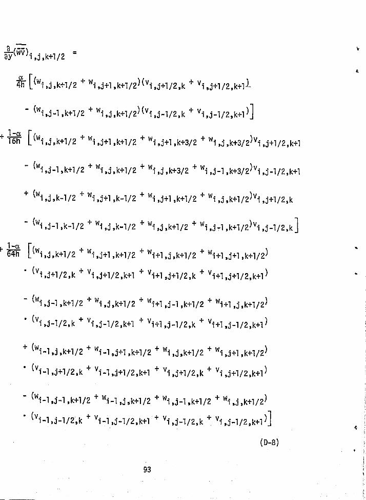
rVO)i,j, k

4

+1/2

a [ (WIs j ,k+1/2 + Wi , j+1 , k+1 /2)(vi, j+1/2 ,k + vi,j+1/2,k+1-)-

(wi,j -1,k+1/2 + wi, j ,k+1/2)(v i, j -1/2,k + vi,j- i1/2,k+1 ) l ,d:r

+ I -a16 ""

rL (w i,j ,k+112 + wi,j+l,k+1/2 + w1,j+l,k+3/2 +

is :.

wi,j,k+3/2)vi,j+1/2,k+1

- (wi, j -1,k+1/2 + wi,j ,k+1/2 + wi, j , k+3/2 + wi,j -1,k+3/2)vi,j-1/2,k+1

(w i,j,k-1/2 + wi,j+l ,k-1/2 + wi,j+l,k+1/2 + wi,j,k+1/2)vi,j+1/2,k

(wi,j -l,k-1/2 + wi,j ,k-1/2 + Wi,j ,k+112 + wi, j -rl:k+1/2 )vi j-1/2,k]

64h [(Wi,j,k+1/2 + wi, j+l,k+1/2 + wi+l,j,k+1/2 + wi+l,j+l,k+1/2)

(vi ,j+1/2,k + vi, j+1/ 2 ,k+1 + vi+l , j+1/2,k + vi+1,j+1/2,k+1)K

- (wi , j -1,k+1/2 + wi , j ,k+1/2 + wi+1 , j -1,k+1/2 + wi+l ,j,k+1/2)

* (vi,j -I/2,k + vi ,j-1/2,k+'I + vi+1 ,j^-1/2,k + vi+l ,j-1/2,k+1) ,s

f +( w i -l, j ,k+l/2 +

wi-1,j+1,k+1/2 + wi, j ,k+11 2 + w iJ+l,k+l/2).

(vi -1 ,j+112,k + vi -1,j+1/2,k+1 + vi ,j+1/2,k + v i ,j+1/2,k+1)

- (w1 -1,j-1,k+1/2 + wi -1,j ,k+1/2 + wi,j -1,k+1/2 + wi,j,k+1/2)(v i - l , j -1/2,k

+ v + vi-1 J -1/2,k+1 i,j-1/2,k vi ,j -1/2,k+1) #

(a-8)f

4-

93i

a ww)1,j,k+1/2

a2 2^4h (w

+W } w1 j,k+3/2 ) (w

i,j,k-1/2 - Wi ,j,k+1/2)

+ 1-a2

64 [('i ,j,k+1/2 + wi,

j ,k+3/2 + Wi+1

,j,k+1/2 + Wi+l, j ,k+3/2)

- (w1,j,k-1/2 + Wi ,j ,k+1/2 + W1+1 , j , r'-1/2 + w1+1,j,k+1/2)2

+ (wi -1 , j , k+1 /2 + Wi -7 k+3 2 + Wi k+7 2 + Wi k+3 2 ) 2

(wi - l , j ,k-1/2 + W1 - 1 , j ,k+1/2 + wi,j,k-1/2 + W1 ,j,k+1/2)2

a + (w1,j,k+l 2 + wi + +w w• 2/ ,j,k^-3/2 i,j+i,k+i/2 3,j^-1,k+3/2)

(w i , j , k-1 /2 + wi k+i 2 + wi +1 k-1 2 + Wi +1 k+1 /2)2

+ (wi , j - l ,k+1/2 + wi,j-1,k+3/2 + Wi,j ,k+1/2 + Wi,j,k+3/2)2

APPENDIX E

PROGRAM TFC (IN PUT, OUTPUT, TAPES= INPUT, TAPE G =OUTPUT, TAPE 9, TAPE 9)C *****,r*****r*************************r^e**,^****************^r*******C * LANGUAGE:FORTRAN COI•IPUTF.R:CDC7600 COI .IPILER:P,UN76, LBL BERKELEY*C * NOMENCLATURE:C * 1•I MESH SIZEC * DT TIME STEPC * UO sMAXIFIUN MEAN VELOCITY IN SHEAR FLOWC * OMEGA ROTATIONC * C TURBULENT MODEL CONSTANTC * FDC FINITEDIFFERENCE COUSTANTC * L NUMBER OF TIME STEPSC ****r**,*************************f*********************x^*********

LARGE PR1(16,16,J6},PI1(16,1G,16),tdAV1=C16,16,16)LARGE U1C16,I6,I9),V1(1Ei,1G,19),!JI(16,IG,19)LARGE RXI.(16,16,16),E:Y1(16,1U,16),RZ1(16, 16,16)DIi1ElISION U(22,22,7),V(22,22,7),!-I(22,22,7)DIMENSION EV(20,20,5),PR(20,20,5)EQUIVALENCE (EV(1,1,1),PI'.(1,1,1))DHIENSION 5X(18, 15, 3),SY(1°,1Ei,3},SZ(18,1I3,3}DIHENSIDtI Rf1G,16),Q[(16,I6)DIMENSION 1!(3},11106},I12(S),TR!?(16, -a),TRI (16,3),EC16)COi•li•10 it/SCE 1 /t^R, Q I , 1I, t i1,1 i2, TR ., TR I , E, I S 1 GN, PA IREAL LAIIBDAPAI=3.141592653589793P;AI 2=PAI *PAI

H2=H*HDT=0.025C=0.24Uu=0. 0a11ECA=0. DFDC=I./3.CI = FD C/11C2= (1.—FDC)/4./E1C3=C*C *llC4=Cl/4.C5=C2/16.C6=C2/4.C7=1. / (112*4. )C;=1./(2. *11)C7=1./H(:11=C1/2.C12-C214.CALL TRRTRI

C----- I .11 TI AL DATA:C ----- SWIROUTI NE I III G OON GEIIERAi ES THE 11. 11 TI .AL VELOCITY FI LLDC •-----ACCURD l NG TO APPEUD I X 13

CALL INICONDO 11 r, =1,16DO 11 J =1,16DO 1 1 1= 1,16RXI ( I , J, i4) =0. 0EtYI(I, J,i;)=0.0

11 CONTI WEC-----FIRST STEP IS ADWICEP. '-3Y EULER iLwTH"ID (ALPHA=1.0),

L1

'i

r

C -----ADAMS-BASHFORTH METHOD 15 USEL THEREAFTER (ALPHA-1.5)ALPHA=1.0

' L=OUSQR=0.0DUDX2=0.0DUDX3=0.0E1lRG=0. 0DIV=0.0

6 M-1Do 2 K=1, 3

t KK=K+16DO 2 J-1,16DO 2 1=1, 15Ul(I,J,Kr,)=U1(I,J,K)

ill ( I , J, 1,K) =ill( I , J, K)2 CONTIHUE

WRITL•(6,102) L102 FORMAT(iH1,1OX,221-INUMBER OF TIME STEP L=, 13)

IIRITE(6,107)107 FORMATC 1:1 ,10;i, U COMPONENT OF VEL FIELD *}

Sf•IALLIN(QRC1,J.),1J1(1,1, 9), 256)DO 44 i=1,16,811RITE(G,106) I

t IIRITE(6,105) (QR0,J),J=1,16)44 CONTI NUE

' !W TE(6,108)108 FORVIAT(1H ,10X, * V COHPONENT OF VEL F I E[.f) *)

S.MALLiFf(QR(l,l),V1t1,1, 9), 256). DO 45 1=1,16,8

WRITEC6,106) I

IJRITE(6,105) {Q!?(I,J),J=I, 1G) `45 CONT I WE

AI TE( G, 109)109 FORMAT(lii , IOX, * W COMONENT OF VEL FIELD *}

S•fALL11I(QRt1,1),!'7l(I,1, 9), 255)DO 46 I=1,16,8WRITE(6,106) I

1 ;•1RITE(6,105) (QR(I,J),J=1,1G)46 CONTIldUE1 IF (1•f. E?.I} GO TO 8

^ ry7GO TO 16

8 00 20 K5=1,7K-K5K2 = K5+13IF(r,Z.GT.16) 1,2=K2•-16

16 SMALL1N(QP,(1,1),U1(1,1,K2), 256)DO 29 J-1,16DO 29 1=1,16JJ =J+3{11=1+3Ut 11,JJ,l:}=QRt1,J}

29 CONT1 NNEslant.LliltQR(1,1),V1{1,1,;:2}, 256)

96 ORIrsIlVAL. PACE

11

i1

OF POOR QUALIM

w

DO 89 1-1,15DO 89 J=1,16JJ=J+3! 1 =I+3V( I I,JJ,K)-11MI,J)

f 89 CONTI fill

! 51•lALL111{QR(I,1),1II{1,1,1:2), 256)DO 99 J=1,1600 99 1=1,16JJ=J+311=1+3tI[! I,JJ,U-QR(I,J)

99 COUTINUEI.!,

C-----EXTEND VELOCITY FIELD PERIODICALLY IN X,Y DMECTIONS.DO 24 J=4, 19U(1,J,1;)=U(17,J,K)

-_.-. V(1,J,K)=V(17,J,K)U(1,J,K)=;I{17,J, Y,)U ( 2, J, K) =U (18, J, K)VC 2, J,K)=V{18,J, K)

* :1( 2, J, K) =tI{ 18, J, K)U(3,J,K)=U(19,J,K)V( 3, J, K) = V(19, J, K)'HC 3, J,,",) =11(19, J, K)U(20,J,K)=U(4,J,K)V( 20, J, 1,)=V(4, J,]'%):•I(20, J, IC) = tI( 4, J, UUC21,J,1,)=U(5,J,I',)V(21,J,K)=V(5, J, K)s1(21, J, K.) =1I(5, J, K)U( 22, .r, K) = U( 6, J, 1:)V(22, J, K) = V( 6, .I, K) a ..;,11( 22, J , .! , == I(E, J, K)

24 CO NT 114UE.D0 22 1=1,22U0,1,0=00,17,K)V ( I , 1, '-0 = V( 1, 17, K).!{ I , 1,K) =11( 1, 17, K)6(1,2,1;)=U(I,18, K3V(I,2,K)=V(I,18,I:)U(1, 2,K)=11(1,18,1-,)U(1,3,K)=U(l,19,K)V(I , 3,':.) =V( 1 , 19, Ii)4(1,3,K)=t!(I,19,K)U(I,20,1,3 =U(I, 4, K)V{I,20,K:)=V(I, IF , K).I( I, 20, K) =11(I,4, K)!1C 1 , 21, K) = U(1 , 5, rt)Vf1,21,K)=V(1,5,K).I( I, 21, K) =;I( 1, 5, K)U(1,22,K)=U(1,6,K)VC I , 22, K) = V( 1, 6, 1,,)

' 22 CO NT I fill 20 CONTI i-IUE F.

ORIGING11 ZS 97

AID. PA .OF PooR

QlaulTi

l_.. S

C-----COMPUTE Tl1E EDDY VISCOSITY COEFFICIENT 1DO 25 Ka2,6DO 25 J=2,21DO 25 1=2,21ICK=K-1JJ=J-1I I^I-1 ffEV( I I, JJ,I: I;)= C3*SQRT (2. *(U(I,J,K)•-U( 1-1,J,K))**2 t

* +2.*(V(t,J,K)-VCI,J-1,K))** 2+2.*(^1{I,J,I:)-1d{l,J,1:-1))**2 l#* +.25*((U(I,J+l,K)-U(I,J,I;)+V(1+I, J,1:)-V(I,J,K))**2* +(U(1-1,J+1,1;)-U(1-1,.1,K)+V(1, J,1'%)-V(I-1, J, 10)**2* +(U(1-1,J,K)-U(1-1,J-1,K)+V(I,J-1, 1:)-V(1-1,J-1, K))**2* +{U(1,J,E.)-U(1,J-1,K)+V{1+1,J-1,l;)-V(I,J-1,Y.))**2* +(V(I,J,It+I)-V(1,J, K)+41(I,J+1, K)-!1(I,J,K))**2* +{V(1,J,K)-V(I,J,K-1)+1'1(1,J+1,K-1)-W(I,J,K-1))**2* +(V(I,J-1,K)-V(I,J-1,K-1)+11(1,J,!:-1)-W(I,J-1,K-1))**2* +(V(I,J-1,1C+I)-V(I,J-1, K)+11(1, J, K)-1{(1, J -1, 1U ) * *2* +(1'1(I+1,J,1")-1,1(1, J, K)+U(I,J,K+l)-U(I,J,K))**2w +{lH(I+1,J,K-1)-1,1(I,J,K-1)+U{I, J,K)-U(I,J,K-1))**2* +01(1, J,K-1)-110-1, J, K- 1)+U(I-1, J, K)-U(1-1, J,K-1))**2* + al ( I , J, K) -W ( 1 -1, J, K) +U ( I - 1, J,K+1)-U(1-1, J. K))* *2))

25 CONTINUEC-----COflPUTE R.;I.S. OF MOMENTUM ERUATIOII (PRESSURE GRADIENT jC-----NOT I11Cl.UDED)

I F(1l. E(1. 1) GO TO 26K=)svO TO 27

2b DO 35 K=2,427 DO 35 J=2,19

DO 35 1=2,39KI.=K-1JJ=J-1 F

11x1-1JI=1J2=1IF(JJ.14E.1) GO TO 58J1=-1J2=-I

58 SSX=* -C4*(CU(1+2,J+1,K+1)+U(I+1,J+1,K+1))**2* -(U(1+1,J+I,K+I)+U(I,J+1, I.+I))* *'2)-05** ((UCI+2,J+I,K+1)+U(I+2,J+2,1,+1)+U(1+1,J+2, 1%+1)+U(1+1,J+I,K+I))**2* -(U(1+1,J+1,1,+1)+U(I+1,J+2,K+1)+U(I,J+2,K+1)+U(I,J+1,K+1))**2* +(U(I+2,J,K+1)+U(1+2,J+1,K+1)+U(I+1,J+1, 1:+I)+U(I+I, J,K+I))**2* -(U(1+1, J, It+l)+U(I+1,J+1,1,+I)+U(I,J+1,K+1)+IJ(I,J,1:+1)) **2* +(U(1+2,J+1,K+2)+U(1+2,J+I,K+1)+U(1+1,J+1,1C +1)+U(I+I,J+I,K+2))**2* -(U(I+1,.J+I,!'+2)+U(I+1;J+1,K+I)+U(I,J+1,K+1)+U(I,J+I,K+2))**2* +CL1(1+2,J+1,K+1)+U(I+2,J+1,i:)+U(I+l,J+1,f:)+U(I+1,.J+1,K+1))X*2* -{ U( 1+1,J+1,Y.+1)+U(I+1,J+1,K)+U(I,J+1,!;)+U(I,J+1,K +1)) **2)

SSX=S'SX-C4** ((U(I+1, - J+1,!t+1)+U(I +1,J +2, 1: +1))*(V(I+2,J+1,1t+1)+V(I+1,J+1,K+1))* -(U(I+1,J,K+1)+U(I+1,J+1,K+1))*(V(I+2, J,K+1)+V(I+1, J,K+1))) - C6* r.(( U(1+2,J+1,K+1)+U(I+2,J+2,1,+1)+U(I+1,J+2,K+1)+U(I+1,J+1,K+I))* ^.* VC 1 +2, J+1,1:+1)* -(U(I+2,1,K+1)+U(1+2,J+1'1'%+I)+U(I+1,J+1,K+I)+U(I+I,J,K+1))*

4R^GTN^.: ;UAIlTy98 Off` gR

66

)Uz'vn{) 2Iood do.el 5ioVa qvlu;)ruo

(I+,1'I+r'z+I)n*•f[*t{11+s•)^1[*,•+il*(I-rr)i^a7^))+ .^TT:1*(C(I+.1'r`T•+•17A+tT+,i'r'Z.+I)A}*({I!+5'}-1!*5'-E€*{I-rf')i^`(}`I^)- ^

((T+;I'T+r'T+I )A+(I+.I'T+P'Z+I )A)*((1f+5')-li*5'+Ii*(T-rr)il OIj) ))*Ofl-(,1,1 `rr ` f I } X S= C :1,!' PP' i I } xf;

(ZT3*t{I+,1`P`I}n-(T+.1'T+P'I)fl-(I+,1'I+P'Z+I)fl+(I+,l'r`Z+I)fl)*{ (11+5 ' )-H*5'0-I1* (T•-PPUVOI J)+

ZI O* ( (T+:I'T+r' i ) n- (I+:i Z+r' i ) n- (T+N Z+r' z+ i ) n+ ( I+.i' I+r'Z+ I) fl)*t {I1+s')-i1*5.0+11•*(I-Pr)i4e-I:1}+cZTZ)*( (;f'T+r' 1 )n-ox li+r'Z+1 )fl+ *

(Z+,1`T+r' i )fl-(T+:I''i+r `1 )n*'Z-(T+,l'T+P'Z+1 )fl*'Z+(Z+.I'I+P`z+I )fl)+ *ITO*(CI+.f'T+P'i)n-(I+;i'i+r`Z+1)n))*({Ii+s')-1,*(T-PP).LVDi3))*P.n*'Z- *

t:1.i Irr I I f) xs= cl,l'rP' I I )xsLOT.(((:i`I+r'I+I)r;-(:1`I+r'Z+1)!i+(;€'I+r'I+i)n-(T+,I'T+f''Ia•I)n) *

* ( ( I-•;1'P'T+ I )A3+( T-5!'r' I )A=1+('A'P'I+ I )A3+ Of "P' I W )- *( (T+,1'T+r'I+1 )I;--(T+.I'T+r'Z+ I )f4+(I+)l `I+P'I+I )fl-(Z+:1'T+r'I+ i )n)

*((T+:1'r'T+I)n:^+(T+:E'€'`i)n^+(;I`r'I+1)n]+{:1'r`I)A7)+ *C (I+,I'r'I+1 )n-(T+,['r'Z+ 1 )A+tT+,;'r'I+ I )n-{I+,I'I+r `I+ I )n) *

*{ (.I'T-r' I )n^+(,!'Y -P'I+ f }A3+t.l'r'T+ I )A1+(:I'r' 1 }A3 )- *(CT+:i'T+r'T+1)A-(I+:i'I+P'Z+[)A^(l+:l `I+r`I+I)n-(I+,'.`Z+P'I+I)fl)

* ((;1'I+r' I }A3+():'T+(''I+ I )A3+(.I'r'I+ 1 )A3+(,1 `r' [ )A3) +C( (T+,;'T+P' 1)fl-(I+,['I+P'T+1 )n)*(N'r' 1 )A?-

(cT+: `T+r'I+I)n-CI+,:'T+P `z+I)n}*(,1'r'I+1}n3)*•8}+ *xss=(;i:;'rr' I i lx^

c c (:1`T+r'I+I )rl+(:1'T+r'Z+I M+(;€`r *I+i )fl+c;€'r'z+i );i)*((T+1;'I+r'T+1)n+(:i'I+r'I+[)n+CT+.1'r'T+I)n+(.I'r'I+i)n)-

{CT+.f'T+r'T+[)fi+{I+:i'I+f''Z+I)!i+(T+,I'P'T+I)!•1+(I+:1'r'Z+1}f;) **{(Z+)1'T+r'I+I)n+(I+)['T+r'I+1)fl+(Z+;1'P'I+1)fl+(T+'r'I+1)11)+

C(.^`Z+C''I+I)fl+{,1'7+r'4+I)fi+(:i'C+P'I+1)T4+(:;'T+r `Z+I)f:) ** ( (I+)i'Z+P'1:+ 1 )n+(:i' Z+P'T+ I }n+( I+:1'T+P'T+ I )n+Di'I+P'T+ I )fl)-

((T+,1'Z+f 'I+[ )fl+(I+,f'Z+f' `Z+I )M+(I+,I'T+P'I+1 )1l+(I+,l'T+r'Z+1 }fi)* ((Z+,f'Z+P'I+I )n+(T+.i'Z+P'T+ 1 )n+(Z+,1'I+r `I+I )n+(I+ i+P'T+ I) n) )

*S- C (•['I+r'I+ 1 )l; **C{I+,1'I+P'I)!l+(,i'T+r'I)n+(:!'I+P'I+I7f1+(I+:;`T+r'T+I)n)-

(I+,1'T+r'I+1 )fl*((Z+.l'I+r'I}fI+CI+.I'I+r`I)n+{T+.{`T+r'I+E)n+(Z•r,;'I+r'T+i)fl)+ *

of T+r'Z+ I )m **((T+.I'I+P'T+17A+(;f'I+P`I+I)n+{;i'T+r'Z+1}fl+(1:+:;'I+f''Z+I)n)- *

(I+?I'T+P'Z+ 1 )fl **((Z+:1'I+P'T+I)n+(T+:1'T+P'I+I)!1+(T+,1'T+r'Z+I)n+(z+;l'T+r `Z+1)n))* *

93-{t(.i'T+r'I+1}ri+C.l'I+P'Z+[)fl)*((I.1'I+r'T+I)n+(;f'T+r'T+I)n)- *((I+,1'I+P`T+1)hi+(T+%1'I+P'Z+I?fl)*((Z+,1'T+r'I+I)n+(T+,1'I+r'I+i)n))* *

ha-xss=xss{({T+,1'r°T+1)A+(I+:1'r'Z+17A+(,I'r`T+1 )A+(,I'r'Z+I}A) *

*{CI+:1`T+r'T+l)n+Cl+.l'r'I+!)ti+(;:'T+r'I+1)na•!.i'r`I+1}n}^• ^'((I+,1'I+r'I+1)A+(I+11'I+r'Z+I)A+C,1'T+r'I+i)At(,['I+P'Z+I}A) *

*((T+N'Z+r'T+I )n+(I+,1'T+P'I+1 )fl+(,;'Z+r'I+I )n+(,i'I+r'I+i )n)+((Z+x`P'I+[)n+(7.+:t'r'z+l)A+(I+,1'P'i+I)A+(T+,f'r'Z+I)A) *

*((Z+,i'I+r'I+I )n+(Z+)i'r'I+i )n+(T+)I'T+f 'T+I )fl+(I+:I'P'T+I )n)-tCZ+,1'T+P'I+1 )A+(Z+%['T+r'Z+1 )A+(T+,I'T+r'I+I)A+(I+.1 I+r Z+I )A)

*((Z+,1'Z+P'I+I)n+(Z+i'I+P'I+i)n+(I+,1'Z+P'I+1)n+(I+,f'T+r'I+i)n))*50-((I+N'P'I+1)A

* { (T+,1'P' I )n+(I+.1'I+P' f )n+(T+,1'T+r'I+ I )n+(T+)I'P'I+i )n)-(I+:; `I+r'I+ I ) A

*{(I+:i'T+r'1)n+(I+N z+r'I)n+(T+:f`Z+r'T+1)fl+(I+:I'I+f'T+1)n)+(I+,I'P'Z+I )A

I

.i

''1 '} Qoa aoCl0 !

{CT+a'Z+PIT+I)A+(T+)l'T+r'T+I)A))I

*to -Ass=Ass(Z**( (T+)I'P'*I+1 )A+(T+)l'T+P'T+I )A+C:I'T+P'T+1 )A+()i'P'I+i )n}-

z** ( (T+N'I+P'T+ l )A+( I+',I'Z+P'I+ I ) n+0l'z+r'T+ I )A+()I'T+r'1+ 1)A )+Z**((Z+)l'r'I+I)A+(Z+)['T+r'I+I)A+(I•r)t'T+P'I+1)n+(I+)['P'I+I)A)-

Z**{CZ+)l'I+r'I+I)A+CZ+%Ii'Z+C'T+I)A+(I+:t'z+r'I+I)A+(1+1111+r'Y+I)n)+Z**( (I+)I'P' I )A+(I+)1'T+f`' I )A+(I+,l'I+r'T+ E )n+(T+:I'r'T+1 )n)-

Z**i (t+:['I+P' I )A+CI+A'Z+P' I )A+CT+;:'Z+P'T+I )A+(t+'rl'I+f''I+I )A}+Z**{ CI+)l0P'I+I )A+(T+::'T+P'T+I )A+(I+N'I+P'Z+I )A+(T+:I'P'z+[ )A)-{

Z**( (I+):'T•+•P'I+ I )A+i T+)1'Z+P'I+ I )A+( T+);'Z+P'Z+ 1)A+(T+)I'T+f''Z+ i )A) )*5a-(z**((T+)l'P'I+1)A+(T+N'I+P'T+I)A)-+

z{(I+:I'I+r'T+i)11+cI+.l'Z+P'I+I)A))*to-Ass=Ass

• ''(`1'T+P' i )n+(`I'Z-PI )n+(N'T+P' I )n)*{(I+)I'T+r''I)A+(I+x'I+r'r+E)n+()['I+r'I}n+(:I'I+P'I+I)n)-

'e{(I+N'Z+P'I+1)n+(I+:l'T+r't+I)n+{A"z+r'T+!)n+(::'T-}r'T+I)fl)M-* C (1+y'I+P'T+ I )A+C I+)l'T+P `z+ I )f,+ ()E `T+P'I+ I )A+()I'I+C'Z+ I )A)+

((z+a'z+r'I)rl+(z^);'T+P'1)n+{T+;1'z+r'I}n+CT+,I'I+r'I)n}*((z+)I'T+r'I)A+CZ+,['I+r'I+E)A+{T+'T+P'[)A+(T+:i'T+r'T+I)A)-

({ Z+`l,'Z+r'I+I )n+(z+:!'T+P'T+ I )fl+( T+)1'Z+P'T+ I )n+(T+%I'T+P'T+ I )fl)((Z+:l'I+P'T+I)A+CZ+;i'T+P'Z+I)n+(T+;I'I+P'T+1)n+(T+;!'T+r'Z+I)n})

fl* ( (T+:I'P' I )A+(T+)t'T+P' I )A+(T+:I'I+P'T+ i )A+(T+)t'r'T+ [ )A)-

(T+N IT+r'T+ I )n*C (I+31'P'T+I )A+CT+)1'I+P'I+I )n+(T+`.I'I+r'z+I )A+(T+)I'r'z+ I )A)+ ^:=

(I+)1'z+rII)fl

*{(T+:I'tl•r' I)n+(I+}t'Z+r' I )A+(I+:!'Z+r'I+1 )n+(T+:i'T+P'T+I)n)-(T+N'Z.+r'I+I)n

*((T+;I'I+P't+l )A+(I+)t'Z+P'T+I )A+(T+;i'Z+P'Z+I )A+CT+)I'T+r''Z+I )A) )90-Ct(T+,I'Z+P'I)7+(T+'T+r'I)n)T+:I'T+r'I)A+(I+x'I+r'I+I)A)-

((I+)1'Z+r'I+I)n+tT+;;'I+P'T+I)^1)((T+;I'I+P'TI)n+(T+:t'T+P'z+l)A))*t3-=Ass

((T+)l'P'T+I )A+{T+)I'T+P'T+I )A+(T+)l'T+P'Z+I )A+(I+%'r'Z+I )A)* Z'*dJ3110*'Z+

(ZTO*C C C:[T+rT+ I )ft-i.[T+rZ+ I )hl-(`trT+ [ )f-(,1rZ+I )rl--^CI+:I'I+r'T+I )f,I+(T+)l'I+P'Z+I )V+{I+)l'P'I+1)11+(I+)I'r`Z+I )h)

^(Crl+s' }-[Ixs-11*(I-rP)1yo1^)+^( (N'Z+P'I+ 1 )11-0 'Z+P'Z+ I )r;- ()I'T+P'T+ I )r;- (:I'T+P'z+ I )r',-

(T+?1'z+P'T+1)P1+(T+:l'z+r'Z+I)!l+(I+)I'I+r'I+1)r1+(T+,['T+r'Z+I)rl)((H+5')-Id*5'+tl*(I-rr)1VC13))+

(zO+TT3)*Ct^'I+r°T+1}r•1-()I'I+r`Z+I)rl-(T+:l'T+r'I+i)!'l+(t+`.l'T+P'z+l}r1)

{tEi+s'on-C)1)I "VP ' I I'rr I I I) xs

-t ^`(zT^*C (fl+^'r'T+t )n+tT+^'r'z+ t }n+{,I'r'I+1)n+{a'r'z+I }n)*(tll+5 •)-llc5'-E1*(I-Pr)IVOI2)-

C (t+:['I+r'T+ I )A+(I+)I'I+P'Z+ I )A+(}i'I+r'I+ I )A+(:1'I+r'Z+ I )A) r;+((II+S')-I1*s'+II^(I-rr).t_traZ^)+( (z+:t'r'I+1)A+cz+)l'P'Z+I )A+(T+;l'r'T+I )n+(T+)l'P'z+1 )A)

*C CI!+S' )-fl*5'-11*(I-Pr)1tl013)-CCZ+,'T+P'T+I)A+CZ+U'T+P'z+1)A+(I+;I'T+r'I+I)A+(T+;1'I+e'z+l)A)

*C(E?+s')-1^*s'+I-I*(T-rr).tnal^)+*...ft+N'P'T+I)A*C(H+S')-H*5'-11*1-PP)IV01d)-

iT+)I'T+P'T+I )A*C {II+5')-11*5'+11*(I-PP)IV013)+f I+:I'P'Z+ I )A*t* C C11+5')-11*5'-li*(I-VP )IVOI3)-

i

* -(V(1+1,J+1,1:)+V(I +1,J+I,Y.+1 })*(:l(I+1,J+I, K)+1.1(1+1,J+2,K)))-05y* *({V{1+1,J+1,K+1)+V([+I,J+I,%+2)+V(1+2,J+1,K+1)+V(1+2,J+1,K+2))** { 1.I( I+1,J+I,K+I)+11(1+1,J+2,Ki1)+1-1(1+2,J+I,1;+1)+W(1+2,J+2,K +1))* -(V(I+I,J+1,K)+V(I+I,J+1,K+I)+V(1+2,J+I,K)+V(I+2,J+1,1;+1))** (:1(1+1,J+1, K)+1-1(I+1,J+2,1')+11(1+2,J+1,.K) +tl(I +2,J+2,K))* +(V(I,J+I,K+I)+V(1,J+1,IC+2)+V(1+1,J+1,1;+1)+VCI+I,J+I,:+2))** (1I{1,J+1,K+1)+tlCI,J+2,K+1)+WI+I,J+1,K+1)+'.!(1+1,J+2, 1: +I)}* -(V(I,J+1,1.)+V(I,J+1,K+1)+`I(I+1,J+1,1.)+VC1+1,J+1,K+M** (I-I(I,J+1, 1:)+:!(I,J+2,[t)+tl(1+I,J+1,.: ) +1d(I+I,J+2,K)))-C6** ((V(I+I,J+I,K+I)+V(1+1,J+2,K+1)+V(I+I,J+2,K+2)+V(I+I,J+1,K+2))** 1J(1+1,J+2,K+1)* -(V(I+I,J+1,K)+V(I+I,J+2,1C)+V(1+1,J+2,Y.+I)+V(I+I,J+I,K+I))** W(I+1,J+2,K)* +(V(I+I,J,K+1)+V(I+I,J+1,1t+I)+V(I+I,J+I,K+2)+V(I +I,J,It+2))*

* -(V(I+I,J,K)+V(I+I,J+I,K)+V(I+1,J+1,K+1)+V(1+1,J,K+I))*

SY( I I, JJ,I:f{)=SSY* +((EV(I,J, 1:)+ EV(I,J+I,K)+EV(1,J+1, Y,+I)+EV(I,J,IC+I)}** (V(I+1,J+1,1C+2)-V(1+1,J+1,1;+1)+,'!{1+1,J+2,f:+1)-:IC1+1,J+I,K +I))* -(EV(1,J,1,)+EVCI,J,i:-I)+EV(1 1+1, 1.-I)+EV(I,J+1,K))** CV( 1+1,J+1,I:+I)-V(1+1,J+1, i:) +tI(I+1,J+2,K)- t-I(1 +1,J+I,1:)}* +3.*(EV(I,J+1,1:)*(V(1+1,J+2, 1:+I)-V(1+1,J+1,;•,-1))* -EV(I,,J,..)*{V(1+1,J+I,1:+1)-Y(1+I, J,K+1)))* +(EV(I,J,1:)+EV(I+I,J,K)+EV(1+1,J+I,i:)+EV(1,J+I, K)}** (VC[+2,J+1,K+I)-V(1+1,.'+1,K+1)+I)C1+1,J+2, IC+I)-U(1+1,J+I,K+1))* -(EV(I,,J,IC)+EV{I,J+1,K)+EVC1-1,J+1, 1C)+EVCI - 1,J,K))** (V{I+1,J+1,K+1}-V(I,J+1,I:+1)+U{I,J+2,1:+1}-U(I,J+I,l:+1}))*C7SY( 11, JJ,I:It)=SY( I I, JJ,::1:)

* -UO*((FLUAT(JJ-1)*11-JI*.5*(1.+J2*II))** * ((V(1+2,J+1,1:+I)-V(I,J+1,K+I))*CII

* +(2.*V(1+2,J+1,I;+I)+V(I+2,J+1,1:+2)-2.*V(I,J+I,K+I)-V(I,J+I,K+2)* +V(I+2,J+1,1:)-V(1,J+1, K7)*C12)* +(FLOAT(JJ-l)*11+.5 :i-,11*.5*(1.+J2*11))** (V(1+2,J+1,l,,+I}+V(1+2,J+2,1:+I)-V(f,J+2,1:+1)-V(I,J+I,K+1))*C12* +(FLOA'f(JJ-1)*11-,5*11-J1*.5*(1.+J2*tl))** (V(I+2,J,l%+I)+V([+2,J+I,K+I)-V(I,J+I,K+1)-V(I,J,K+1))*C12)* -2. *OtIEGA*0.25** (U(I+1,J+1,K+1)+U(1+1,J+2,1.+1)+U(I,J+2,K+I)+U(I,J+1, 1:+1))SSZ=-C4*

* ((t1(1+2,J+I,K+1)+11(I+1,J+1,If+1))*M1+1,J+1,1:+2)+U(I+I,J+I,K+1))* -(t IC 1+1,J+1,1C+1)+;!(1,J+I,K+1))*(U(1,J+1,K+2)+U(I,,J+l,1%1+1)))-05* *((1IC1+2,J+1,1C+I)+t1(1+1,J+I,::+I)+1I(1+2,J+2,i; +1)+11(1+I,J+2,K+1) )*

* (U(I+1,J+1,K+2) +U(I +1,J+1,K+1)+U(I+1,,J+2, 1,+2)+tJ(1+1,J+2,K+1)}* -(1I(I+1,J+1,K+1)+11(I,J+1,K+1)+^l(1+1,J+2,1C+1)+Il(i,J+2, 1:+I)}** (U(I,J+1,1t+2)+U(I,J+I,K+I)+tJ(I,J+2,1:+2)+U(I,J+2,K+I))* +(.1(1+2,J,1:+I)+:!{i+1,,J,K+I)+1.1(1+2,J+I,K+I)+;I(1+1,J+1, Y.+I))** (U{1+1,,J,i:+ 2)+U(1+1,J,K+I)+11CI+I,J+l,lt+2)+U(1+1,J+I,K+1))

K+1)+1.1(1,J, f.+I} 4•;1(1+1,J+1,K+1)+1l(I,J+I,K+1))** (U(isJ,K+2)+U(1,J,1;+I)+IJ(1,J+1,}:+2)+U(1,J+1,K+I}))-CS** {(tl(1+2,J+I,K+2)+11(1+2,J+1,f:+I)+'I(1+1,J+I,K+1)+U(i+1,J+1,K +2)) ** U( 1 +1, J+1,K+2)* -(tI([+1,J+I,K+27+tJ(1+1,J+1,K+I)+tl(I,J+1, t:+I)+t•I(I,J+i,1C+2))*

' * U(I,J+I,K+2)* +01(I+2,J+I,f;+1)+tIC1+2,J+I,,;)+;1(l+1,J+I, K)+.!(Ij1,J+1,K+1))*

ORTGR4AI, PAGE is 101

OF POOR QuA.LITY

WITooh• 40

ZOLqj 1413W&

11

Z-)l9 W II !I 1 7S'AS I X S 30NVACV----- ^

3f3W IINO35^tZTO*{tT+)I'T+P'1)I;-(I+)1'f'`I}11-(T+)I'T+r'Z+i) III +(T+y'r'Z+I)r1) *

CCr;+S')-I1 5`0-I?*CT-rr)IV013)+Z13*((I+VZ+r'I)F.-(I+>'I+r'I)11-(I+31`Z+P'Z+1)I1+(T+)1'T+P'Z+I}1.)

( (1i+5' )-II*S O+FI* CI-rr ).LVO Id)+

(Z13*( (%I'I+r, I t "N II+l,'Z+ I )r•;+{Z+)i'T+P't)F1-(T+'N T+r'I)Ii*'Z-(I+';'T+r'Z+I)Ii*'Z4 Z+y'T+rIZ+I)II)+TI0*( (I+:i'I+P' I )r1-•(I+)E'1+r'Z+I )I.) )*C M+S')-I1*(I-PP)J.MJ) )*011-

{N%,1 17'P' 1 I )ZS- {y:1'PP I I I )ZSl0* ({ ( C)I'T+P'I+ I )r•1-(T+)I'T+r `'I+ I )r1)* ()''r' I )A3-

( {I+)1 `T+P`I+ I )11-(Z+)I'T+r'T+ I )Ii)*tl+:l'P' l )A3 )*'P+ *((1+)l 'P IT+ I )A-(Z+)l'P IT+I )A+{T+U'r'I+ 1 )I1-(I+)I'1+r'T+1 }r•1) *

*((T+:I'P' I )A3+011'P' I )A3+()l'T-P' I )A3+{T+)1'T-P' I )A3)- *{ (T+)1'I+P'T+ I )A-- (Z+)1'T+P `T+ I )A+(T+A'I+P'T+ I )11--(T+:'.'Z+r'T+ I VA)

*( CT+VT+P` I )A3+(VT+r' I )A3+()t'P' I )A3+(T+:3`r' I )A3)+ *C CI+?1'I+r' i )n-(Z+:I'T+r' I )n+(T+%I'T+P' I }Fi"{T+)I'T+P'T+ 1 )I1) *

1A3+()1'P' 1It )A3+(I+%r'P IT- I )A3)-*(CT+^'T+P'I+!)fl-tZ+:l'T+P'T+I)n+(T+:1'T+r't+l)ri•-(I+:I'I+P'Z+I?I1} *

^(i)I'r'!)A3+()l`P`I+I)A3+(t+)i'P'I+E )A3+(I+)1`P'I)A3))+ *ZSS- ()E)l'rr I 1 I) ZS

tZ**C(I+)I'I+r'T+I)r1+()i'I+P'T+I)ii+{I+:l'r't+I)ri+t)1'P'I+l)!•1)- *Z**((Z+:1'I+P'I+1)t1+CI+)1'T+r'I+i)r•1+(Z+:!`P'I+[}I•.+CT+)!'r'I+I}!1)+ *Z*(CI+N'Z+P'I+1}1.1+();`Z+P'T+1)l1+CT+^'I+r'I+1)li+()I'T+P'I+l)I )-

Z**((Z+)f'Z+r'I+I)I•i+CI+)I'Z+P'T+l)Yi+(Z^°).'T+P'T+!)I1+{T+;I't+r'I+1)11)+ *Z**t tl+:{'I+r'T+1)r.+(71'T+P'T+ i }z?+{I+;{'I+P' 1 )I1+()1't+r' 1 )f+1)- *

Z**L(Z+;<'T+P`T+I}I1+(T+:1'I+P'I+I)M+(Z+%l`T+P`I)Fi+(T+)I'T+.P'I M)+Z**((I+il'I+P `Z+ I )f1+C)l'I+r'Z+ 1)ri+tT+)1'T+P'I+l )11+(t'I+P'T+! )I1)- *

Z**((Z+;{'I+r'Z+1 )P1+CI+:I'I+P'Z+! )I•!+(Z+?1'I+r'T+I }F1+{T+)1'T+I''I+! )r•i) J **50-CZ**t(I+:t'I+P'I+i)!•1+()1'I+P'I+!}rl} *

-•Z**{ tZ+:1't+P'I+ I )r1+CI+)I'I+P'L+ 1)!1) }**to-ZSS=ZSS

C(T+)1'P'T+1 )A *((I+:I'P`T+I)fi+(t+:i'I+P`T+I}I.1+(:1'I+P`T+I)h1+{)1'P'T+I)I1)- *

CT+)1'T+r'T+ 1 )A *((t+)l'T+P"1+1)r•i+(T+)I'Z+P'T+1)r1+(:1'Z+r'I+I )1'1+C)I't+r'T+t )vo+ *

C Z+A If, IT I )P, **{{Z+)1`r'T+I)In+(Z+'l'T+r'T+I)f1+(I+)I'T+P`T+IVA+(I+)1`r'T+I)I.1)•- *

( Z+)1't+r'I+ 1 )A

*E(Z+)l'T+P'I+I)I1+(Z+N'Z+P'T+I)A+{I+)1'Z+r'T+I)I1+(T+)i'T+P'T+I)M))**93-C ((Z+)1'P'I+I )A+CI+),'PIT+I )A+(Z+)1'P' I )A+(I+:!'P' I )A) *

*C(T+;i'I+P'T+1)rt+(I+:r'r'T+I)I1+(T+)I'T+P'1)M+(I+%I'P`I);1)- *((Z+x'I+r'I+I)A+(T+)! " I+r'T+I)A+(Z+)1'I+P'I)A+(I+)I'T+rII)A) *

'F{(T+N'Z+P'T+I)A+(T+N'I+r'T+I)F1+(i+%I'Z+r'1)I1+(T+:1'T+P'I)I.1)+ *((Z+N'P`Z+!)A+(T+n `P'Z+I)A+(Z+)1`r'T+1)A+(T+)l'rIT+I)A) *

*((T+,,

IT+P`Z+I)h+(T+il If' 'Z+I)r1+('C+:;'T+P`I+i)ri+(I+:['P'T+1)M)-• *

{(Z+)1'T+P'Z+I)A+(T+;;°I+P`Z+I)A+(Z+:i'T+r'T+1)Ai(T+`I+r+r'7+1)A) **((T+)1`Z+P'Z+1)I.1+{T+)I'T+P'Z+I)fA+(T+:['Z+P`T+i)M&(T+:l'T+r'T+I)r1))* *

SO- C({Z+:I`r'T+IIA+(T+%I'r`T41}A}*C(T+:I't+P'T+I•)11+(T+N'rIT+1)11)- *((Z+N't+r'T+I)A+(T+)1'I+r'T+I)A)*{(T+N'Z+r'I+I)I1+(T+:1'T+r'T+!)I.1)) *

*^r0-ZSS=ZSSc ct+a `t+r' I )n

*C(t+)['t+r't)r•1+()I'T+P'l)I.1+(:I't+r't+l)I•i+{T+)!'t•^P't+l)F1)- *(T+)1'T+P'T+I )n

f

Ly'^

i

F

i

L'

SHALLItJ(Q{(1,I),U1(1,l,ii), 256)51t.1LLIN(Qf'.{i,I),fZX1{1,1,iI}, 25G)DO 60 J=1,16DO 60 11,16QI C E , J}=fIl C 1, J)^(ALPIJA*5X (I+1, J+1, I.1-. 5 *QRC I . J)) *^]T

60 CONTINUESltALLOUT(QI(1,1),UI(I,I,t1), 256)DO 12 J*1,16DO 12 1-1,16!11 (I,J)=SX(1+I,J+1,2)

12 CONTINUESHALLOUT(QI{1,1) ,RXl(1,1,M), 256)SMALLIWCQI (1, 1),VI(1,1,H), 256)St•IAL I IPJCQR(1,11,RY1( I I "), 256}DO 61 Jx1,16DO 61 I=1,16Q1 (I , J) =III C I, J)+(ALPIIA*SY(1 +I, J+1,1:)-. 5,tq

61 CONTINUESNAL LOUT (Q1 (1, 1),VI(1,1,M) . 256)DO 14 J=1,16DO 14 1-1,16.Ql({,J)-SY(1+1,J+I,2)

14 CONTI NUESt4ALLOUT(Q1 (I,1) ,RY1(1,1,11), 256)Sf iALL1iJ{QI(I,1),tl1(1,I,ti), 256)SIIALLII•ICQR(1.,1),RZI(1,1,tt), 256)DO 62 J=1,16DO 62 1=1,16Qt C I , J) -Q1 (I , J)+(ALPIIA*SZ(1 +1, J+1,1C)-. 5*0

62 GOHTI14UESHALLOUT(QI(1,1), 141C1,1,M), 256}DO 15 J=1,16DD 15 1=1,16Q1(I,J)=SZ(I+1,J+1,2)

15 CONTI NUE:S11ALLOUT{QI{1,1) ,RZl(1,1,f,i), 256}

C-----FORI! THE R. I.S. OF POISSON EQUATION'CIO=I./(DT*ALPHA)K=4DO 30 J=4,19DO 30 1=4,19JJ=J-3111-3ZI(II,JJ)= (UCI,J,tI,) -I1{I-I, J, I:}+VC I, J, K) - V

QR(l I,JJ)-III (I I,JJ)*CIO+* (SX(I-2,J-2,I1-2)-SX(I--3,J-2,I:-2)+SYC{-2,* SZ(I-2,1-2, I:-2)-Sl.(I-2,J-2,1:.3}}*C9

C---- CJtIPUTE DIVERGENCE, TURBULENT ENERGYDIV=t)IV+QI (I I,JJ)IJSQR-U (I , J, [,) **2+US{IRDUD X-(U (1 , J, t;) -U ({ -1, J, I:) )'f k lDUDX2=DUDX**2+DUf)X2I)UDX3 =I)UDX**3+DUDX3EtlR{s = E1J^G+U(1 , tJ, IC) **2+V(1, J^ E:)* *2+1'!C I , J,^l;

ORIGINAL . PAG4, ^SOF POOR QUALITY 1 03

30 CONTINUEIF (M.EQ. 9) GO TO 9GO TO 7

9 1JRITE(6,I03)103 FORIMAT{ li 1 , IOX, *D l VERGENCE V *) '

<ITE (6,104) Id104 FORMAT(1Ii ,10X, 21111=, 12 )

DO 19 1-1,16,9WRITE (6,106) 1

106 FORMAT(Iii ,IOX,2]ii-,12)WRITE(6,105) (QI{I, J),J=1,16)

105 FORMAT (2X, 3 (E16. 7) )19 CONTI NUE7 SllALLQUT(QR(l,l),PR1(1,1,11), 256)

C-----SIII FT U, V,1J, SX,SY,SZ 011E PLANE IN Z DIRECTIONDO 32 K-1,6DO 32 4=1,22DO 32 1=1,22

V(I,J,K)-V(l,J,K+1)11(I,J, K)=:1(I,J,K+I)

32 CONTINUEDO 34 K=1,2DO 34 J=1,18DO 34 1=1,18SX (I, J, I:)=SX(I,J,11%+I)SY( I,J,K)=SY( I, J,1;+1)SZ( I , J, 1,)=SZ( I , J, K+I)

34 CONTI NUEIF(li.EQ.16) GO TO 3811=11+1K2=K2+1GO TO 1

38 DO 55 K=1,1600 55 J=1,16DO 55 1-1,16Pll(1,J,f,')=0.0

55 CONTINUEC----- 111VERT THE POISSON EQUATION 13Y SU IUMOUTi NE PSWEQN

CALL PSfIEQN',•JRITE(6,110)

110 FORIIAT(lii ,IOX,* PRESSURE FIELD *)SIIALLIil((jR(l,l),PRI(1,1, 9), 256)DO 47 1-1,16,81JRITE(6,106) IWRITE(6,105) ((^R(I,J),J=1,16)

47 C011TI NUEC-----ADVAIJCE PRESSURE GRADIENT IN Ti ME

M-1K4=15

50 DO 41 K=1,31:3 =r, 4+KIF(K3.0T.16) K3=K3-16I F(K3.OT. 16? 1;3=1%'3-16S' iALi.IN{t1t',(1,T),PI;I{I,I,i:3}, 256)

104 OF p00R I VA `

a

DO 42 J=1,16DO 42 1=1,16JJ=J+1I I =1 +1

PR(I1,JJ,K)=QR(1,J)42 CONTINUE

C-----FXTE141) PRESSURE FIELD PERI OD I CALL. IN X, YDO 39 J=2,17PR( 1,J,X)=PR(17,J,K)PR( 1S, J, K) = PR(2, J, K)

39 CONTINUEDO 43 1=1,18PR(I, 1,K) = PR(1, 17,K)PR( I,18,l')=PR(I,2,K)

43 CONTINUE41 CONTINUE

K=2Do 54 J-1,16DO 54 1=1,16Z1:(1,J)=-(PR(I+2,J+1,K)-PR(I+1,J+1,K)) *C9

54 CONTIMUESlIALL11.1(01 (1, 1),U1(1, 1,H ), 256)D 52 J=1,16DO 52 1=1,16;21 (1 , J) = -1I ([ , J) +QP (1 , .1) *ALPiiA*DT

52 CON]TI HUESMALLOUT(l1 (1, 1),U3.(I,1,13 ), 256)SMALL ItJ(Q1(1,1),RXZ(1,1,H ), 256)DO 53 J=1,16DO 53 1=1,16QI ( I , J)=Z1(I,J)+2P.(I,J)

53 CO WTINUES1IALLOUT(n1(1,1),RX1(1,1,11 ), 256)DO 64 J=1,16DO 64 1=1,16:1a(I,,1]=-{PR(I+1,J+2,K)-PR(1+1,J+1,K

64 CONTI14UES1tALL111(')1(1,1),V1(1,1,l1 ), 256)DO 65 1 [1, 16DO 55 J=1,16ZI (1, J) =rl I (I, J)+QI;(I, J)*ALPItA*DT

65 Ci!I1TI NUE511ALL0UT(Itl(1,I),V1(1,1,11 ). 255)SllALLlll(Ql(1,1),RY1(I,1, t 4 ), 256)00 63 J=1116DO 63 1=1,i6!11(I,J)= 11 1(I,J)+(Ir;(I,J)

63 CONT I NUES^tALLOl1T(Q!(1,1),RY1C1,.,h1 ), 256)DO 74 J=1, 16PO 74 1 =1, 16QR(I,J)=-(PI:(1+1,J+1, 1;+1)-P"(1+1,J+1

74 CONT114UESMALLHIMI(1,1],;l1(1,1,11 ), 256)70 75 1=1,16'

ORIGINAL PAGE IS 105OF POOR QUALITY;'

DIRECTIONS

D0 75 J-1,16RI (I, J) =QI (I, J)+QR(I, J)*ALPHA*DT

75 CONTINUESHALLOUT(QI 256)SMALLIN(QI (1, 1),RZI{1,1,11 }, 256)DO 73 J=1,16DO 73 11,16

73 C014T1 NUEStiALLOUT ( QI(1,I),RZ1 ( I,1,M ), 256)IF(M.EQ.16) GO TO 401i =t 1+ 1K4=Y.4+1GO TO S0

40 L=L+1C---- - COI• -PUTE TAYLOR 111 CROSCALE, SKEWNESS

LAI.IBDA=SQRT ( USQR/DUDX2 )DUDX2=DUDX2/ 4096.DUDX3=DUDX3/ 4096.SKEW=;DUDX3/DUDX2**1.5ENRG-ENRG/ 4096..IRITE(6 , 111) SKEW,EHR G,C11V,LAHBDA

III FORHAT (// , IOX,1011SKEHNESSX =, E16. 7, 5X, 7H ENERGY=, E16. 7,* SX,11111)1 VERGENCE=, E16. 7, 5X, 8HLAI ^BDAX=, E16. 7)

D I V=0.OENRG=0.0I]SQR=0.0DUDX2=0.0DUDX3=0.0IF(L.GT. 0) ALPHA=I.SIF(L.GT. 0) GO TO 78GO TO 6

78 CONTINUESTOPEND

i

SUBROUTINE PSNEQNC ********+r*****#********t******^t**********,^***r*****r*****,r,e****w*C * POISSON SOLVER FOR 16 CUBE POINTS WITH PERI011IC B.C. BY FFTC * ALGORITHMC * VIAVE(I, J,K) IS THE WAVE NUMBER K' DEFINED IM CHAPTER I IIC * ISIGN = I, ISIGN =— I ARE FOR FORKARD AND BACKWARD TRANSFORMS,C * RESPECTIVELYC ********x*,r***r**,^t****************************r****^r*****r,t*******

L A RGE PR1(IS,16,I6),Pll(16,16,16),1IAVE(16,I6,I6)DIMENSION N(3),h.1(6),t92(6),TRR(16,3), TRI (16,3),E(I6)DIMENSION QR(16,16),QI(16,16)COHMON/SCAT/QR, QI , N,M1,M2, TRR, TRi , E, I SI GN, PAIli=1./I6.

li3=H2*HNN-16NN3=NN*NN*NNC1=1./NN3C2=PAI/NNC3=1./H2ISIGNa1CALL FFTXCALL FFTYCALL FFTZ,DO 26 K=1,16DO 25 J-1,16DO 26 1=1,16 PR1(I,J,IU=PR1(I,J,K) *C1/IJAVE(I,J,K)Pi l(I,J,K) = PI l(I,J,K)*CI/VIAVE(I,J,K)

26 CONTINUE= PRZ(I,1,1)aO.G

Pll(I,l, l) =0.oISiGN=-1CALLFFTZCALL, FFTYCALL FFTXRETURN'END

F

J

SUBROUTINE FFTXwwwwwww+^ww*wwwww*www***+twwtww*ww**tww*rrf**www**w*w*wwt^rwwwwwwtf*ww*

C * FAST FOURIER TRANSFORM IN X DIRECTIONC * 1 S I GN-I, I SI GN--1 ARE FOR FORWARD ANT) SACKWAR[) TRANSFORMS, }C * RESPECTIVELY. THE FORWARD TRANSFORM RETURNS 16 TIMESC * THE REQUIRED RESULT. FOR DEFINITIOM OF FFT SEE APPENDIX CC wwttwwwtwttwww**www,eww**war*w•kw*w*wwwwwww*wwww*wwww*sr*,r*tww*wwww*t#w

LARGE PR1{1G, 36 ,15),PIi(i6,16,^C},i#r;VE(16,15,16)DIMENSION N(3),t4l(6),t•12(6),TRR(16,3),TRI(15,3),E(16) -DIMENSION Qn(I8,16?,QI(16,18) ^'COtiMOt!/SCIt/QR, Ql,tl,til,t•12,TRR,TRI,E, I SI GN, PA)DO 200 K-1,16DO 2$0 J=1,16DO 100 M-1,3JJ=H(t*i)KK-0

5 ti=KK+JJ+11tK=i I+JJ-1DO 10 I=11,KKL=1 -JJZ= -PR1( L, J, K) u

T=-PIl(L,J,K)PR1(L,J,Y,)=PRI(I,J,K)+PR1(L,J,K)PIl(L,J,K)=Pil(i,J,K)+Pil(L,J,K)Z-PR1(I,J,K)+ZT=P11(I,J,K)+TPRI(I,J,K)=Z*TRR(1,t1)-T*TRI(I,M)* ISIGN

10 PI1(1,J,K)=Z*TRI(I,M)*[SlGt4+T*TRR(I,M)IF(KK.NE .16) GO TO 5

100 CONTINUEDO 110 12,16, 2PR1(1,J,K) PRI(I,J,K)+PR1(1-1, J, K)

110 PII(I,J,K) P I I I, J, K)+P11{I-I, J, K)D0 120 1=1,15,2PRI(I,J,K)=2.*PR1(1,J,K)-PRI(I+I,J,K)

120 P11(I,J,K)=2.*Pll(I,J,K)-PIl(1+1,J,K)DO 20 L-1,611-x11 { L)i 2 =G12 (L)DUM1 -PR 1(1 2, J, K) iPR1(12,J,K) =PR1(11,J,K)PRI(1 1, J, K) =DUMIDUMI=P1 1( 12, J,K)PI 1(12,J,i;) =P11(I 1, J, K}Pi 1( 11, J, 10=DUMI

20 C011TI NUE200 CONTINUE

RETURNEND'

1 08

7

a

CCC

5

10

100

IIO

120

20200

k

7

SUBROUTINE FFTY#tF****t*t*##*t**#*f#*#4t*t*##*#***#*#*t***#*****#***t^***#* *tktttitttt* FAST FOURIER TRANSFORM IN Y DIRECTION t#*ttt**#***ttt***##ttt**####**ttt*,r**,r*t*#*^****tt**##*#***t**+r***t

LARGE PRI(16,16,16),P1l,(16,16,16),IIAVE(16,16,I6)MMENSION td{3),111{6),142(6), TRR{I6,3),TRI (16,3),E(16)DIMENSION QR(I6,16,),QI (16,16)COMMON/S C11 /QR, Q I , N, MI, M2, TRR, TR I , E, I S I GN, PADO 200 1,=1,16DO 200 1=1,16DO 100 t1 n 1, 3JJ=N(M)KK-OI I =F:K+JJ+1f:K^I l+JJ'In 0 J=1I,Y.KL =,,- JJZ=—PRIG, L, K)T--PI 1(I, L,K)PRI(I,L-,K)-PP.1(I,J, K)+PRI(I,L,K)PI1(I,L,K)=PII(I,J,I:)+PII(I,L,K)Z=PP.1(I,J,K)+ZT=PII(I,J,K)+TPRI ( I , J, K) -Z*TRR(J,14) — T*TP I (J,19 * I SIGNP11(1,J,K) =Z*TRI (J,1;)*I5IGIf+T*TRP.(J,"4)IF(Y UE".16) GO TO 5CONTINUEDO 110 J=2,16,2PR1(I,J,KJ = ^P^1(I,J,Y,}+PR1(I,J—I, K)NI1(I,J,1;) =— PI1(f,J,K)+PI1{i,J-1, K)DO 120 J=1,15,2PRI(I,J,11%)=2.*PRI(I,J,K)—PP,I(I,J+I,K)PI I(I,J,K)=2. *PI I(I,J, I:)—PI I( I,J+I,K)DO 20 L=1,6I I =14 I ( L )12442(1-)PU1II-PRI (I, 1 2, K)PRI(I, 1 2,1C) = PRI(1, I I, K)Pr! I ( I , 11, K) =DUM10U1II=PI 1( I, 12,K)P1I(1,12,K)=P1I(I,f1,K)

CONTINUECONTINUERETURNEND

r

ORIGINAL, PAGE IS

109-OF POOR QUALITY,

1

-

y

s

SWROUTi NE FFTZC w**,r; ************,r**^r*w***^r*,r****#***t********t*^r,t+r^r ** rc*********tr**

! C * FAST FOURI ER TRANSFD,",`t IN Z DIRECTIONI C ,r***t,t** w,t***w,r****.t****,rt*,r******,r,r**,r*,r** ,r***,r************,r******L4RGE PR1(16,16,16),PI1C1G,16,IG),IIAVE(16,16,16)DIMEI.15ION N(3),tII(G),1.12(6),TRR(I6,3),TRI(16,3),E(16)DIMENSION QR(16,16),QI (16,16)COttt9ON/SCM/QR,QI,M ti1,M2,TRR,TRI,E,ISIGN,PAIDO 200 1=1,16DO 200 1=1,16

f. DO 100 P1-1,3JJ=N(M)KK=0

5 1I=KK+JJ+1KY.=1 I+JJ-1DO 10 K=1 1, KKL=K-JJZ--PRI( I . J, L),:T=-PI 1( 1 , J, L)PRI(I,J,L)=PRI(I,J,K)+PRICI,J,L)P11.(I,J,L)-Pf1(I,J,K)+PII(I,J,L)Z=PR1(I,J,K)+ZT a P I I( I, J,K)+TPRI(I, J, K)=7.*TRR(K,t1)-T+TR1 (K,tt3 *I SI GN

10 PII(I,J,K) = Z*TF.I(K,H) I S I Gtl+T *TPR C K, Y!)

IF(KK.NE .16) GO TO 5100 CONTI14UE

DO 110 K=2,16,2PR1(I,J,l:)=-PR1(1,J,K)+PRI(1,J,1;-I)

110 PI IC I, J,K)=-PII I, J, K)+PI IC I,J,.[%-1)DO 120 K-1,15,2PR1(I,J,K)=2.*PR1(I,J,K)-PR1(I,J,K+l)

120 PIICI,J,Y.)=2.*P11(l,J,K)-P11LI,J,1:+I) `'DO 20 La1,6I1=til(L) {:I2=t12(L)DUt11 =PRI ( I , J, 12)_PR1f1,J,i2)^PR1{1,J,1I)PR1(I,J,I1)=DUti1DUMI=P11(I,J,12)PI IC I, J,12)=PII{i,J, 11)PI IC I, J, 11)=DUM1

20 CC) MTI MUE t>`200 CONTIt1UE

RETURNEND

,r

PaxAL

F;

`

110y

y

4

SUBROUTINE TRRTRIC wwwwwwwww w***w*ww***wwwwwwwwww*wwaw w***ww*www* *w*w*w*www**** w* wwwssC * INITIATION OF THE TRIGONOMETRIC FUNCTIONS TRR,TRI REQUIRED FOR xC * THE FFT SUBROUTI PIES, AIM WAVE (THE WAVE NUMBER K) FOR PSNEQN

fC **w**www,rw*+r****w**w*w*wwwww*******,,r*wwwww**w******wwww**+tw*ww****

LARGE PR1(16, 1f,Ifi),PII(16,16,i6},1l.AVE{i6,1fi,16)DIMENS1011 N(3),Ii1(6),fi2(6),TRR(16,3),TRI (I6,3),E(16)DIMENSIO!! 'QI:(Ifi,lfi),QI (16,16)CO? IMO tl/SCt1/QR,QI,N,htl,1-i2,TRR,TRI,E, ISIGN,PAIDATA tit/2, 3, 4, 6, 8,12/ADATA M2/8, 5, 13, 11,15,14/DATA

H2-H*ta' NN-16

C2=PAI/NNC3=1./H2F1{I]a3N(2)ti4 j

N(3)r-2DO 24 K=1,16 .DO 24 J=1,16 t.90 24 1-1,16WAVE (I,J,K)=- 4.*(SIN (C2*E(I)}**2+SII)(C2*E(J))**2

. * +SIN(C2*E(K)) **2) *C3CONTINUE

-..-41 WAVE (1,1,1)=1.0 .

' 60 lo ti . 1, 3L=N(M). J=1

30 K=J+2*N(M)-1 ! iDO 20 I-J,KIF(I.GT.L) GO TO 22

TRi (I,h^}ap.GO TO 20

22 TRR( 1,11)=COS( PAI *( I -1)/N(ti) )I T11.I(I,;i}=-SIN(PAI*(I-1)/N(M)}

20 CONTINUE ^.IF(K.EQ.16) GO TO 30L=K+N(M)J= +1

fGO TO 3010 CONTI IIUE

RETURNENO

331

ORIGINAL PAGE 16

OF POOR QUALITYi` .

SUBROUTINE INICONC tttttttttttttwtw*,rw*w*w,tw+*w* t****ttt *t*tt *t *w **ww*tt*tt *wt**#*wtttC * INITIATION OF A RANDOM FIELD WHICH SATISFY CONDITIONS SET INC * APPENDI X B. THE TWO REQUI REP Fl ELDS TO START . III TH AREC * GENERATED IN SUBROUTINE RANDPIC * SUBROUTINE SPECT3 EVALUATES THE THREE —DIMENSIONAL ENERGYC * SPECTRUM OF THE GENERATED FIELDC ttttt*tww***tw**twwttw *ttt*ttt** twit*ttttwww*twtwwwwtttttttttttt *t

LARGE PRI(16,16,16),PI1(16,16,16),4'rAVE(16,16,16)LARGE U1(16,16,19},V1{16,16,19),411{16,16,19)LARGE U2(16,16 ,18),V2(16,16,18),412(16,16,18)DIMENSION QR(16,16),QI(16,16)DIMENSION SR(16,16,6),SI (16,16,6)DIMENSION N(3),III(6),I.12(6),TPR(16,3),TRI(16,3),E(16)COrlr•ION/SCM/QR, Q1, N,Ii1,M2, TRR, TR1, E, I S I GN, PAIH-1./16.iiN=16.HN3=IiN*HH*HNCALL RANDPIARG=2. *PAI 11+NDO 70 K=1,9LL-K+9SfdALLIN(SR(1,1,1),U1(1,1,K), 256)SMALLIN(SI(1,1,1),U1(1,1,LL ), 256)SHALLIN(SR(1,1,2),VI(1,1,K), 256)SMALLlN(SI(1,1,2),Vl(1,l,LL ), 256)SMALLIid(SR(1,1,3),1-41(1,1,10, 256)SHALLIN(SI(1,1,3),411(i,1,LL ), 256)SMALLIFI(SR(1,1,4•),U2(1,1,K), 256)VALLIr•4(SI(1,1,4),U2(1,I,LL ), 256)SPIALLIN(SR(1,1,5),V2(1,I;K), 256)SMALLIN(SI(1,1,5),V2(1,1,LL ), 256)SI.IALLIN(SR(1,1,6),ti12(1,1,K), 256)SHALLIN(S1(1,1,6),4'i2(1,1,LL }, 256)KK=K-9DO 72 J-1,1600 72 1=1,16JJ=J-111=1-1IF(J.GT. 8) JJ=J-17IF(I.GT. 8) 11=1-17ARG1=ARG*11TRC1=l.—COS(ARG1)TRSI=S I N(ARGI)ARG1=ARG*JJTRC2=1.—COS(ARG1)TRS2=SIN(ARG1)ARGI=ARG*KKTRC3=1.—COS(ARG1)TRS3=SIN(ARG1)A=-rRCI*SR(I,J,4)+TRC2*SR(I,J,5)+TRC3*SR(I,J,6)13=TRS1*SI(I,J,1)+TRS2*SI(I,J,2)+TRS3*Si(I,J,3)C=TRCI*SI(I,J,4)+TRC2*SI(I,,1,5)+TRC3*SI(I,J,6)r)=TrS I*SR ( I , J, 1)+TR52*SP. ( I , J, 2 )+TRS3*SR ( I , J, 3)E1=SR(I,J,I)**2+SR(I,J,2)**2+S"(I,J,3)**2E2=SR(I,J,4)**2+SR(I,J,5)**2+SR(I,J,G)'**2

OWGI -AL PAGE

112 mF Poog, gUAL

A.

4

E3-S1(I,J,1)**2+SI(I,J,2)**2+SI(I,J,3)**2E4=SI(E,J,4)**2+SI(I,J,5)**2+SI(I,J,6)**2E5=SR(E,J,1)*SRff,J,4}+ST;(1,J,2)*SR(I,J,S)+SR(I,J,3}*SR(I,J,6)EG=SICI,J,1)*St(I,J,4}+SECS,J,2)*S!(I,J,S)+SICI,J,3} *51(I,J,6}EEE=(EI+E2+E3+E4)12.T)DDnA*B*C*n!F(DDD.IIE.0.0) GO TO 71 ,.BCB=A*C E ``

!F(B.EQ.0.0.ANn.BBBJ4E.0.0) GO TO 75CCC=B*n r°iF(C.EQ.0.0.,ATIC.CCC.,'lE.0.0) GO TO 77IF(C.EQ.O.O.AI)n.n.EQ.O.O.AII0.B.h1E.O.0) GO TO 79lF(A.EQ.G.O.AtID.B.EQ.O.O.AND.C.tIE.0.0) GO TO 200IF(A.,IE.O.O.AtIO.B.EQ.O.O.AIIn.C.EQ.G.O.AND.n.EQ.0.0) GO TO 210 .._...:_IF(A.EQ.O.O.At)D.S.E(I.O.O.AtIP,.C.IE!?.O.O.At4D.D.t$E.0.0) GO TO 220IF(A.' tt')IE.O.O.At4D.B.EQ.O.O.A'•.C.EQ.O.O.AIID.P.NE.0.0J GO TO 230IF(A.EQ.O.O.ATID.O.EQ.O.O.AtID.C.EQ.O.O.At4D.D.EQ.0.0) GO TO 81

71 BETA=RGEII(X1)IF(3ETA.£Q.G.0) GO TO 71

771 GAt1A=A/B*3ETAF1=EI+D**2/C**2*E4F2=2.*BETA*E5-2.*GAtIA*D/C*L•GF3=3ETA**2*E2+GALA**2*E3-EEEF4=F2*F2-4.*FI*F3lF(F4.GT.0.0) GO TO 772BETA=BETA/2.GO TO 771

772 ALPITA-(-F2-SQRTCF4))/2./F1DELTA=-D/C*ALPHAGO TO 73

75 GAHA=RGEfl(X2)I F (GA19A. EQ. 0. 0) GO TO 75BETA=31A*GAMAF1= El +r)**2/C**2*E4F2 = 2. *!)ETA*E5-2. *GAt1A*P/C*EE6F3=BETA**2*E2+GAfIA**2*E3-EEEF4=F2*F2-4.*FI*F3IF(F4.LT.0.0) GO TO 75ALPHA=(-F2-SQRTCF4)}/2./FIDELTA=-D/C*ALPHAGO TO 73

77 nELTA=RGEM(X3)IF(I)ELTA.EQ.0.0) GO TO 77ALPHA=-C /D*DELTAF1=E2+A**2/B**2*E3F2=2. *ALPHA*E5F3=ALPIIA** 2*E1+DELTA**2*E4+2.*ALPIIA*nELTA*EG-EEEF4 = F2*F2-4.*1: 1*F3 }IF(F4.LT.O.0) GO TO 77 tBETA=(-F2-SQRT(F4))/2./FIGAITA=BETA*A/T3GO TO 73

79 ALPIIA-RGEHCX4)0ELTA=nGEW(X5)IF(ALP1fA.C(1.0.0.OR.I)ELTA.EQ.0.0) GO TO 79 .

779 F1=E2 +4**2/8**2*E3

ORIGINAL PAGE IS 113 {

OF POOR QUALITYf

F2=2.*ALPHA*E5F3=ALPIIA**2*EI+DELTA**2*E4+2.*ALPIiA*DL•LTA*E6-EEEF4=F2*F2-4.*F1*F3IF(F4.GT.0.0) GO TO 780ALPHA-ALPHA/2.nELTA=DELTA/2.GO TO 779

780 0ETA=(-F2-SQRT(F4))/2./FIGAt1A=BETA*A/BGO TO 73

200 BETA-RGEN(X6)GAMA=RGEN(X7)IF(BETA.EQ.0.0.OR.GA14A.EQ.0.0) GO TO 200

201 FI=EI+D**2/C**2*E4F2=2.*CBETA*E5-GAt4A*D/C*E6)F3=BETA**2*E2+GAt,4A**2*E3-EEEF4=F2*F2-4.*FI*F3IFCF4.GT.0.0) GO TO 202SETA=BETA/2.GAMA=GAMA/2.GO TO 201

202 ALPHA=(-F2- SgRT(F4))/2./F1DELTA=-P/C*ALPHAGO TO 73

21G LAMA=RGEN(X8)DELTA=RGEN(X9)'SETA=O.OIF(CIA11A. EQ. O.O. DR. DELTA. Er2.0.0)Gol TO 210

211 F4=(EEE-G,A!to**2-E3- DELTA**2*E4-2.*GAfIA *DELTA*EG)/E11F(F4.GT.0.0) GO TO 212GA13A=GAMA/ 2 .I;ELTA=DELTA/2.GO TO 211

212 ALPIIA=-SQRTCF4)GO TO 73

220 GA3IA=RGEM(XI2)DELTA=RGEN(XI3)ALPHA=0.0IF(GAtiA.EQ.0.'O.OR.DELTA.EQ.0.0) GO TO 220

221 F4=(EEE-GAt4A**2*E3-DELTA**2*E4-2.*GAt-1A *DELTA*E6)/£2tF(F4.GT.0.0) GO TO 222GAMA-GAHA/ 2.DELTA=DELTA/2.GO TO 221

222 RETA=-SQRT(F4)GO TO 73

230 5ETA=0.0ALPHA-0.0GAMAFRGEN(XI4)

r:

OF

Irl

GO TO 232231 DELTA-(-F2-SQR'T(F4))/2./F1

GO T4 7381 CONTINUE

DELTA-0.0BETA-0.GALPHA=0.0GA11A=,0.0

73 SR(I,J,I)=ALPHA*SR(1,J,1)+BETA*SR(I,J,4)SI(I,.J,1) =GAI ,1A*SI(I,J,1)+DE• LTA*S1 (I,J,4)SR(I , J, 2) -ALPFIA*SR(I , J, 2)+BETA*SR(I , J, 5 )SI(I,J,2)=GAtIA*51(I,J,2)+DELTA*SI(I,J, S)SR(1, J,3)=ALPHA*SR(I, J, 3)+BETA*SR(I, J,6)SI(I,J,3)=GAIIA*SI(I,J,3)+DEI.TA*SICI,J,6)

72 CONT; PPESHALLOUT(SR(1,1,1),Ul(1,1,K), 256)SIIALLOUT(SI(1,1,1),U2(1,1,K), 256)SPlALLOUT(SR(1,1,2),V1(1,1,K), 256)SHALLOUTCS1(1,1,2),V2(1,1,K), 256)SMALLOUT(SRU,1,3),1•11(1,1,K), 256)SPALLOUT(S1(1,1,3),1,12(1,1,^0, 256)

70 CONTINUEISIGN:-1DO 74 K=1,9M-KSIIALLEN(QR(1,l),U1(1,1,K), 256)St•IALLIIJ(QI(1,1),U2(1,1,K), 256)IF(I,I,EQ, 9) i•-M-16144 =1A+8SMALL0UT(QP 1, 1),PI31C1,1,MM ), 256)SIIALL0UTCQ1 1,1),PI1(1,1,MM }, 256)

74 CONTINUEDO 76 K=10,16LL-18.1:DO 76 J=1,16DO 76 1-1,161F(I.EQ. 9. OR. J.EQ. 9) GO TO 1JJ=18-J11=18-1IF(JJ.EQ.17) JJ-1IP(II.EQ.17) 11x1PR1(II,JJ,LL)=PR1(I,J,K)Pl l(1 I,J,I,LL)=-PI1(I,J,K)GO TO 76

1 PR1(I,J, LL) =0.0P11CI,J,LL)=0.G

76 CONTINUECALL FFTZCALL FFTYCALL FFTXDO 78 K=1,16DO 78 J=1,16DO 78 1-1,16Ul(1,J,K)=PR1(I,•1,K)

78 Cr) 14T1 NO DO 84 K=1,9

ORIGINAL PAGE IS 115

OF POOR QUALr

M-K256)

SMALLIWQI (1,1),V2C1,1,K), 256)IF (hi .EQ. 9) M41-16

SMALLQUT( QR(1, 1) PR1 C 1, 1, MM 256)SMALLOUT ( Q 1 1, 1),P 11 C 1, 1,MM 256)

84 CONTINUE00 86 K=10,16LL=18—KDO 86 J=1,16DO 86 1-1,16IF(I.EQ. 9.0R.J.EQ. 93 GO TO 2JJ=18—d

IFCJJ.EQ.17) JJ=1IF(II.E(I.17) HalPR1(11,JJ,LL)=PR1(1,J,K)PI I( I I , J J , L L) = -P 11 1 J , KGO TO 86

2 PRI(I,J,LL)-O.OPI 1C I, J, LL) -0. 0

86 CONTINUECALL FFTZCALL FFTYCALL FFTXDO 88 K-1,16DO 88 J=1,16DO 83 1=1,16VIC I , J,r,)=PR1(1 J,K)

89 CONTINUEDO 94 K-1,9McKSf4ALLtfJ(QR(1,I),11I(1,1,K3, 256)SMALLPI(QI(I,I),1'{2(1,I,K), 256)IF(M.EQ. 9) 1441-16

SMA L LO U T ( QR ( 1, 1) , PR I ( 1, 1, MM 256)S? I A L LO UT ( Q I ( 1, 1) , P 11 ( 1, 1, MH 255)

94 CONTINUEDO 96 K-10,16LL-18—KDO 96 J=1,16DO 96 1=1,16TF(I.EQ. 9.OR.J.EQ. 9) 00 TO 3JJ-18—d11=18-1IF(JJ.EQ.17) JJ=1IF(I1.EQ.17) 11-1PR1( I I , JJ, LL) =PRI( I J, QP11(f I %JJ,LL)=-PI 1( 1 "ill,%)GO TO 96

3 PRI ( I J, LL) -0. 0P11(1 J, LL) =0. 0

96 CO NT I fit) ECALL FFTZ

QA'ALF.116 fJ

a.

,k.CALL FFTYCALL FFTXDO 98 K-1,16PO 98 J-1,16DO 98 I41,164,11(I,J,K)=PR1(I,J,K)

98 CONTINUECALL SPECT3RETURNEND

SUBROUTINE RANDMC *****w wwwwwwwwww*w*****,r*********w**w*ww****w***ww*w+r**w**w***w*#;*C * INITIATION OF TI-10 RANDOM FIELDS REQUIRED FOR I NI CONC wwwwwwwww***,r*,t***w*w,rw*ww*^r***^rw**,ew*ww*ww******w,t****w******#****

LARGE PRI(16,16,16),PII(16,'V.6,16),:-rAVE(16,16,16)LARGE U1(16,i6,19],VI(I6,16,i9),'.JI(I6,16,193LARGE U2(16,16,18),V2(16,16,18),"12(16,16,18)DIMENSION QR(16,16),QI(15,16)DIMENSION 5R(I6,I6,6),SI(16,IG,6}PiMENSION II (3),111(6),fi2(6),TRR(16,3),TRI (16,3),E(I6)COhi19Ot1/ S CH/QR, Q I , N, I11, M2, TRR, TR I , E, ISI GN, PA IDIMENS1014 EN(14)

C-----EN IS EM, THE THREE-D 1 mctis I OrTAL ENERGY SPECTRUM, AND IS GIVENe C-----AS A FUNCTION OF K AT 2*PAT, 4*PAI, 6*PAI, ETC.

DATA EN/.52,I.5,1.3,.96,.66,.46,.33,.23,.16,.105,.072,.05,.032,.0/ritl=l6.ARG=2. *PAI /IiN00 20 Ka1,9KK-K-9DO 10 J#1,1600 10 1 -1, 16JJ-J-1IF(J.GT.8) JJ=J-17Ilxl-1iFCI.GT.$)II=I-17IF(II.EQ .O.AIID.JJ.EQ.O.AM1ID.KK.Eil.0) G0 TO 10Y=RGEN(X)ZETA=2.*PAI*YAl=l.-C0S(ARG *I1)A2=1.-COSCARG*JJ)A3=1.-COS(ARG*KK)R=SQRT(A1**2+A2**2+A3**2)PHI=ACOS(A31R)IF(A1.NE.0.) GO TO 5I.F(A2.GT.0.0) TIiETA=PAI/2.

r I NA2. LT.0.0) THETA=--PAI /2.

pRIGINAL PAGE ISQF POOR QUALITY 117

ti

I F(A2. EQ. 0.0) TliETA = 2. *PAI *YGO TO 2

5 CONTI NUETHETA=ATAN2( A2,A1)

2 CONTINUtAMAG=SQRT(FLOAT(I1*1I+JJ*J,.)+KK*rK))*2.*PAI19N=AMAG/(2. *PAT )

1'aP1=WNI WIIP1=1141+1ABSVEL = C EIIC IVIN)+(EN ( 119NP1) — ENC I WN) ) *(1914 -119N) } / ( 2. *PAT *AMAG**2 )Y1=RGEN(XI)VELR=SQRT(YI*ABSVEL)VELI=SQRT((1.—Y1)*ABSVEL)U1(I,J,K) =—(COS(ZETA)*COS(PFll)*COS(ThiETA)+Sltl(ZETA)*SI14(THETA))

• *VELRV1(I,J,K) -(—COS(ZETA)* COS(Pill )*SIN(TIiETA)+SIN(ZETA)*COS(THETA)3

• *VELR191(I,J,K) =COS(ZETA)*SIN(PHl)*VELRUi(l,.1,,;+9) =—(COS(ZETA) * COS (PHI) *COS (THETA)+SIN{ZETA)*SIN(THETA))• *VELIV1(I,J,K+9) =( —COS (Z ETA) *COS (PH-1)*SIW THETA)+SIN(ZETA)*COS(THETA))

• *VELIW1(I,J,K+9) =COS (ZETA) *S I WPM *VELI

10 CONTINUE20 CONTINUE

vltl,l,a)=a.aI11(1,1,9) =o.0U1(z,1,18)=a.0V1( 1, 1,18)-0.0J1{1,1,18)=a.000 60 K=1,9KK-K-900 50 J=1,16DO 50 1-1,16JJ =J-1IF(J.GT.8) JJ=J-17I1^1-1IFCI,G7.8)II^I—'71 F (I I . EQ. 0. AN1) . JJ. EQ. 0. Aran . K1,. EQ. 0) GO TO SO-Y=RGEN(X)ZETA=Z.*PAI*YAl=SIN(ARG*Il)A2=SIN(ARG*JJ)A3=S1N(ARG*KK)P.=SQRT(A1**2+A2**2+A3**2)Plil =ACOS(A3/R)IF(A1.NE.0,) GO TO 6IF{A2.GT.0.0) T1iETA=PAI/2.IF(A2.LT.O.u) TIIETA=-PAI/2.IF(A2.[Q.0..0.) THETA=2.*PAI*YG0 TO 4

6 CONTINUETl lETA =ATAM2 (A2, A1)

It CONTI NUEAMAG=SQRT(F LOAT( I I * I I +JJ*JJ+1:K*KK)) *2. *PAI

ORIMAh PAGE ISO.vl

118 0: QL

A

r , 11 r

t

Y

c

WN-AmAG/(2.*PA1)IWN-0IWNP1KiV1N+1ABSVEL-(EN(II•IN)+(EN( IWNP1) — EM( IWN))*(l!N—IWN)}/(2- *PA I*)VIAG**2)Y2=RGEN(X2)VELR-SQRT(Y2*ABSVEL)VELI=SQRT((1.—Y2)*A3SVEL)U2(I,J,Y.) m -(COS(ZETA) *COS (PH I) *COS (THETA) +SIN(ZETA)*SIN(THETA))

• *VELRV2(I,J,K) =(—COS(ZETA)*COS(P]II)*Sit](TliETA)+SIN(ZETA)*COS(TIIETA))

• *VELR112(1,J,K) -COS(ZETA)*S1I1( Pill )*VELI,112(I,J,K+9) w - (COS (Z ETA) *CO S(PHI}*Cf)S(TH ETA) +SIN(Z ETA) *SIN(THETA))

• *VELIV2(1,J,K+9) -( — COS(ZETA)*COS(P!lI)*SIM(THETA)+SIN(Z ETA) *COS MIETA))

• *VELI112(1,J,K+9) -COS(ZETA)*SIH(PHI)*VELI

50 CONTINUE60 CONTINUE

U2(1,1,9)=0.0V2(1,1,9)-0.0W2(1,1,9)=0.0(12 (1, 1,13)x0.0V2(1,1,18)=0.0112(1, 1,18)0.0RETURNENO

0

A

SUBROUTINE SPECT3C ww**www*ww*w**w*w*www*www**w****wwww*w*#***w****wwwww***, t**********C * EVALUATION OF THREE—DIMENSIONAL ENERGY SPECTRUMC wwwwwww***ww**ww* w*www**w*,r**ww*ww**,**w*********,r*w,r *ir****+rw***w*w

LARGE PRI(16, 16,16),P11(16,16,16),ENERGY(16,16,16)LARGE U1(16,16,19),V1(16,16,19),1l1{16,16,19)D114ENSION QR(16,16),QI(16,16)DIMENSION N(3),t11(6),M2(6),TRR(16,3),TRI(16,3),E(16)COtdt•101-1/SCAII QR, Q I , F1,111, P12, TIIR, TR I , E, I S I GN, PA IPAl2=PAI*PAIH-1.116.H2=Ii*HI.i3-H2*HNN-16NN3=11N*NN*NNC-0.6

C-----TRANSFORMATION OF VELOCITY FIELD TO WAVE NUMBER SPACE, ANDC--- FORMATION OF THE TURBULENT KINETIC ENERGY

1SIGN=1DO 10 J-1,16DO 10 1-1,16QI(I,J)=0.0

10 CONTINUEDO 12 K=1,16TIALLIN(QR(I,1),UI(1,1,K), 256)St1ALLOUT(QR(1,I),Pltl(1,1,K), 256) qSf4ALLOUT(QI(1,1),PII(1,1,K), 256)

12 CONTINUECALL FFTXCALL FFTYCALL FFTZDO 14 K-1,16DO lit J=1,16DO 14 1=1,16PRI(I,J,K)=(PRI(I,J,K)/lit-13)**2+(Pl l(I,J,K)/NN3)**2

14 CONTINUEDO 16 K=1,16s"11ALLIN(QR(1,1),PRI(1,1,K), 256)St!ALLOUT(QR(I, 1), ENERGY( 1, 1,K), 256)

16 CONTINUEDO 20 .1=1,16DO 20 1-1,15QI (I,J)=0.0

20 CONTINUEDO 22 K=1,16S11ALLIN(QR(1,1),V1(1,1,K), 256)SMALL0UT{QR(I,1),PRI(1,1,K), 256)SMAI.LOUT(QI(1,1),PI1(1,1,K), 256)

22 CONTINUECALL FFTXCALL FFTYCALL FFTZDO 24 K=1,16DO 24 J=1,16DO 24 1=1,16PRI(I,J,K)=(PR1(1,J,K)114P13)**2+(PII(1,J,IC)/NN3)**2

ORIGINAL PAGE IS1.20' QT` `POOR QUAD

r

,1

24 CONTINUEDO 26 Ku l, 16SMALLIN'(QR(1,1),PR1(1,1,K), 256)SHALLIN(QI(1,1),ENERGY(1,1,K), 256)DO 28 J=1,16DO 28 1-1,16Q1(1,J)=QI(I,J)+QR(I,J)

28 CONTINUESMALLOUT(QI(1,1),ENERGY(1,1,K), 256)

26 CONTINUEDO 30 J=1,16DO 30 1=1,16QI ( 110-0.0

30 CONTINUEDO 32 Kn1,16SI.IALLIrl(rlP.(1,1),111(1,1,K), 256)St1ALLOUT(QR(1,1),PRI(1,1,K), 256)St-1ALLOUT(QI(1,I),P11(1,1,K), 256)

32 CONTINUECALL FFTXCALL FFTYCALL FFTZDO 34 Ka1,16DO 34 J=1,16DO 34 1-1,16PR1(l,J,K)=(PR1(l,J,K}/NN3)**2+(PII(1,J,K}/NN3)**2

34 CONTINUEDO 36 K=1,16St,iALLtt4((IR(I,I),PP,ICI,I,K), 256)SMALL IN(QI(1,1),ENERGY(1,1,K), 256)DO 38 J-1,16DO 38 1=1,16QI(I,J)=(QI(1,J)+QR(I,J))

38 CONTINUESIIALLOUTCQI (1,1), ENERGY(1,1, K), 256)

36 CONTINUEC-----EVALUATIOFI OF THE 3-D ENERGY SPECTRUM

11RITE(6,100)100 FORHAT(III ,10X,*Ti1REE-DIf .iE1-1S1ONAL ENERGY SPECTRUM*)

MalEE=0.011N=FLOAT (M-1) *2. *PAILL=I1!RITE(6,101) WN,EE

101 FORMAT(1H ,10X,2:IY,=,F6.2,5X,511E(K)=,EI6.7)DO 42 M-2,15V1t1=FLOAT(M-1)*2. *PAiEE-0.0 ,RADP=WN+PAIRADI-1=11N-PAILL=ODO 44 K=1,16S14AI.L1tl(2R(1,1),ENFRGY(1,1,K), 256)00 44 Ja1,I6DO 44 1 ml,16KK=K-1

ORIGINAL PAGE IS 21OF POUR QUAD

R .

!

L

r1F.

IF(K.GT. 8) KK=K-17JJ=J-1•IF(J.GT. 8) JJ=J-1711=1-1IF(I.GT. 8) 11=1-17R2=FLOAT(11*11+JJ*JJ+KK*KK)RR-SQRT(R2)*2.*PAII F(RR. LT. RADP. AND. RR. GE . RAD11) GO TO 45GO TO 45

46

LL-LL+1EE-EE+QR(I,J)

45

CONTINUE44

CONTINUEEE=EE/(FLOAT(LL))EE-4. *P A I *C*EE*IIN*WNWRITE("x,101) WN,EE

42

CONTI I OECALL ', RRTR IRETURIEND

s: 1

SAMPLE OUTPUT

1HRFE.OI MENSIOM L £ NF R GY SPECTRUMKa n,00 E(K)a OrKa 6,2 A F(x)s 4.1003845F.03Ku i^,57 E(K)x 4,?9M346AE-02Kx 16, R 5 E (K)e tr?7F?AOQE•02Ka 25 8 43 F(K ) a l.n59? ,iRF-07Ke 31,42 F ( R): 7,u2Aa617E^A;RE 37,70 E ( K)v 5,0153?nSE.03Re 03,9a E(K) r 3F7u?2405r.01Ke 50,27 E(K)s 2PSQP4915EWOAKe 56,55 FM lr6?_O G?11E.03Ka 62.85 F ( g) L 4.4052204EwoaKs h4,12 F(K)e u.a53!?Fi7UFrOt1Ka 75 p 40 E(K)e 3r70Qt2g1EwOuKa 91 68 F(x)* 1,u62154fE•04xr 87.96 €(K)r 2,l2Q9P72E.04

r

^ ^, ASE ^.^

O

123

N

P

S

^, b

gLl"PrP 0P TI ME $7E p Lr 0U C04 PDUFNT nF VEL xi<:Ln

In 1-2.857013E.02 -?.4747339E - 07 2;t5 7 1S5'5 E +02 1. 002010 E.O2 3.3752706Ew02 wj.bt76S9 aE*02 +. I.33 OA430t-oe •3,0043927E.02

-5.051)727 7E-D? »?. g B g6102F.n2 .3;05527 4 6 6.02 -1,4314a gbF.o2 r1.9253 435E wO2 »0.35960576-02 .1.10736 4 3E-02 2.9174775°-02

In 9

-1.n gg 0 ggE-02 8.58463 o tf-03 S;A638267E:02 7.314:6;46. 42 3.5F435n5E-0'c 2.25t5 A55E-Oa 2,30516 9 1E-02 2.713Zh"3e-02

-2.uB A a52`E-A ?1.4550951!"+C2 1.1678625E..02 -1.K8 9 5 4 1?K-D3 -2.1354 7 36E . 02 »A.0308S4 BE-03 -;,ADC A 99FE»42 *3.070u101^-02V CnKAONEN7 Vv VEL FIFLnIr I

-7,99U06h.E.03 »1.3g29724E•02 w?;015250AE.02 -3.79?46OlE-02 -S,(;+696 g 1 4 E-02 -3.n293187F-02 1,1577?04E-02 2.5772654E-02

?.341AFF u E-02 2.1652726E-03 3. 0 071224E..02 7,f785 0 02E-02 5.29642 a 1Erd2 5.7079720E-03 -2.11 97A E-02 -S.9112P20E-r2Ir R

2,7120lb3E-02 2.7?l A7 2 7E • 02 2 *g 3 g 0 p euE.02 6 n 1 M24 4 n 9E- 0 2 9.0AO2b9CE.02 6.b72 a 22 u E-D2 2.393726'1E+02 1-,8283POr,E-n3

S, g 711 1 r i6E . 03 •3.A4425bRE.O3 -7;3574722E.03 -n.A6295OaE-02 *5,5512829E OP .2..3 4 23091E-02 •t,631au43E-03 3-10336.9E-O29 Cn4 PONEVT G P VEL FIELDis 1

w1.A56o1 pS F - p 3 2.6A1A4n4? . p2 1;011049a;O2 9.324b55nE . 00 8.50172u5L-03 .1,2303 0 0 7 E-02 -3,AOAU051E•r3

1 i 999n 7 3^F . 02 3.g28gY7^E.02 -5.1&bO g81E.. 03 .1.5564772E-02 t.5gCn3O2£- 42 1.?DS3977Ew02 -1,6675A39E-Ce

I+s a3,603A T I A E-02 -2 . 355835 . 5 .02 -3f966I 15u1E: p 2 rA.27AO713E»02 .I.S57 4457E - 02 2,3902135E - 62 u,162r ++ 33=•e3

1,5b5537tl-o2 3,227 R 7t3E.02 2.73330Z 1i E.02 6. A 1Al3QAE+Oc" 0.911OR71E .0 2 5.41724C. 5F-02 3.0124581E-02 5,1730714tw^2

^II v E AI GENCE v11 2 9To 1

-3.1 07 4 4 2?E-l u -3„OE aA 065Ewlo .di61A527rE.1a . -3,7343u a n2-14 -3.S07oA 5 n F. 1 u1;776356`1E-Ln 1.4230655£-! a6,754t56CE-14

1.6 4 3001E .. 1 4!. 0 ?1^ 11^+36r14 L. - 1,776y5RQ£ - la +2.1316? E1 2E-1 4 -5.32 g 07 p5E-!A .j.u210A55E .14 "1.105427+16-15

Ir 9

7.1054?7rE.15 1. a 53 ag 2SF-t n0; 3.5527?372-I5 0, :5 6643n1RE-j4 j.99A4714F • j4 5a773j5g7tw14

n, 92 4390?F- 1 4 3.01 944 66E-14 . 1..210855 (=,t 4 •3.5527j37E• 15 0. -7.105n27nE-15 7 n 10S4214E . 15 4,4737942E-14

pG E55URE FIELDI n I

4 n 16b21ebE,.0 46,8 0368336.O u3,902504 c. E.04 1.5836A37E.04 i.890122OErO4 2,727744 7E-04 0.0115030E .0 0 -5 n r$5566rE-O6

wt,79288u u E.OQ 1.7S4 FSL -O4 `6. A 03326tE.G5 -1.nA17n136 . 0 4 +2.P'I r•2b2f Ew0 42.;2b72b8EopG .2.723bA78F..04 -2.6?13916E-04

Ir 9

1,hS4756nE .0 Gh.17a4136r . 04 tr42707bAE. .04 -4.SO A 6u ?+,e-04 .8 . 61.j205 a E -O4 .o ^5ta5hR8ti -04 -S.113658 Af-0u 4.5265A M-05

30RZ4503'c . 04 0.14a5alAE -04 w1,A47463RE-O4 - 7.83669?bE-04 -8.602365uE -Oa t.063n926E-04 8.6a73833E- 0 42.126P526E.04

S KEWIhE85xs w4,8392a08E-O3 ENERGY. 2,7576261EwD3 D2VEPa NCEX .i;6507Il9E-io

LAHSDAx n 9.4Z50444E-02

6 y 4

r,

REFERENCES

Arakawa, A., 1966, "Computational design of long-term numerical integrationof the equations of fluid motions: I. Two-dimensional incompressibleflow," J. Comp. Phys., Vol. 1, 1, p. 119.

Batchelor, G. K., 1953, The Theory of Homogeneous Turbulence, CambridgeUniversity Press. t

Batchelor, G. K., 1967, An Introduction to Fluid Dynamics, CambridgeUniversity Press.

Champagne, F. H., V. G. Harris, and S. Corrsin, 1970, "Experiments onnearly homogeneous turbulent sn ear flow," J. Fluid Mech., Vol. 41,part 1, p. 81.

Clark, R., 1975, Ph.D. Thesis, Thermosciences Division, Dept. of Mech.Engrg., Stanford University, to be published.

Cochran, W. T., et al.,1967, "What is the Fast Fourier Transform?,"Proc. IEEE, Vol. 55 1 10, p. 1664

Comte-Bellot, G. and S. Corrsin, 1971, "Simple Eulerian time correlationof full and narrow-band velocity signals in grid-generated 'isotropic'turbulence," J. Fluid Mech., Vol. 48, part 2, p. 273.

Corrsin, S., 1963, "Encyclopedia of physics," Vol. VIII/2, (Ed. Flugge, S.} and C. Truesdell), Springer-Verlag, Berlin.

Deardorff, J. W., 1970, "A numerical study of three-dimensional turbulent,channel flow at large Reynolds numbers," J.Fluid Mech., Vol. 41 , , part2, p. 453.

_. ^.

Deardorff, J. W., 1971, "On the magnitude of the b^:bgrid scale eddycoefficient," J. Com . Phys., Vol. ?, p. 120.

Deardorff, J. W., 1972, "Numerical investigation of neutral and unstableplanetary boundary layers," J. Atmos. Sci., Vol. 29, p. 91.

Fox, D. G. and S. A. Orszag, 1973, "Pseudo sy, ectral approximation totwo-dimensional turbulence," J. Comp._ "hys., Vol. I1, p. 612.

Fromm, J. E., 1963, "A method for computing nonsteady incompressibleviscous fluid flows," Los Alamos Sci. Lab. Rep. LA-2910.

Gear, W. C., 1971, Numerical Initial Value Problems in Or dinary Differ- 'sential Equations,, Prentice-lla , New Jersey.

Halleen,R. M. and J.P. Johnston, 1967, "The influence of rotation on flowin a long rectangular channel--an experimental study, "Report MD-18,Thermoscience Division, Dept. of Mech. Engrg., Stanford University.

125

I

.I

}

f{

II

Harlow, F. H. and J. E. Welch, 1965, „Numerical calculation of time-dependent viscous incompressible flow of fluid with free surface,"Phys . Fluids, Vol. 8, p. 2132.

Harris, V. G., 1974, "Experimental studies in a field of nearly homo-geneous sheared turbulent flow," Ph.D. Thesis, Johns Hopkins university.

Hinze, J. 0., 1959, Turbulence, McGraw-Hill, New York.

Johnston, J. P., 1974, "The effects of rotation on boundary layers inturbomachine rotors," NASA SP 304, p. 207.

j Kwak, D., W. C. Reynolds, and J. H. Ferziger, 1975, "Three-dimensionaltime dependent computation of turbulent flow," Report No. TF-5,

$= Dept. of Mech. Engrg., Stanford university.

Leith, C. E., 1965, "Numerical simulation of the earth atmosphere,"Methods in Computational Physics., Vol. 4, p. 1.

Leonard, A., 1974, "On the energy cascade in large-eddy simulations of 7

turbulent fluid flaws," Adv. in Geophysics, Vol. 18A, p. 237.

Lilly, D. K., 1965, "On the computational stability of numerical solu-tions of time-dependent non-linear geophysical fluid dynamicsproblems," Mon. Weather Rev., Vol. 93, 1, p. 11.

b

Lilly, D. K., 1966, "On the application of the eddy viscosity conceptin the inertial sub-range of turbulence," NCAR Manuscript No. 123.

Lilly, D. K., 1967, "The representation of small-scale turbulence innumerical simulation experiments," Proc. of the IBM ScientificComputation Symposium on Environmental Sciences, IBM Form No.320-1951, p. 195.

Orszag, S. A., 1969, "Numerical methods for the simulation of turbulence,"Pis. Fluids, Suppl . II, p . 250.

Orszag, S. A., 1971a, "Numerical simulation of incompressible flows withinsimple boundaries. I. Galerkin (spectral) representation," Studiesin Applied Math., Vol. 1, 4, p. 293.

Orszag, S. A., 1971b, "Numerical simulation of incompressible flows withinsimple boundaries: accuracy," J. Fluid Mech., Vol. 49, p. 75.

Orszag, S. A. and G. S. Patterson, 1972, "Numerical simulation of three-dimensional homogeneous isotropic turbulence," Phys. Rev. Lett.,Vol. 28, 2, p. 76.

Reynolds, W. C., 1975, "Computation of turbulent flows," Report No. TF-4,Mechanical Engineering Department, Stanford university.

126

Richardson, L. F., 1927, "The deferred approached to the limit, part 1,single lattice," Phil. Trans., A226, p. 299,

Rotta, J. C., 1951, Zeitschrift fur Ph sik, Vol. 129, (I), p. F47.

Rotta, J. C., 1962, "Turbulent boundary layers in incompressible flow,"Progress in Aeronautical Sciences, Vol, 2, (Ed. Ferri, A.,D. uc emann, an Sterne), ergamon, Oxford.

Schumann, U., 1973, "Ein verfahren zur direkten numerischen simulationturbulenter stromungen in platten-und ringspaltkanalen and fibersein andwendung zur unterschung von turbulenzmodelien," NASA Tech.Trans. TT F 15, 391.

Smagorinsky, J., 1963, "General circulation experiments with the primitiveequations. I. The basic experiment," Mon. Wea. Rev., Vol. 91, p. 99.

Smagorinsky, J., S. Manabe and J. L. Holloway, 1965, Mon. Wea. Rev.Vol. 93, p. 727.

Tennekes, H. and J. L. Lumley, 1972, A First Course in Turbulence,M.I.T. Press.

Williams, G. P., 1969, "Numerical integration of the three-dimensionalNavier-Stokes equations for incompressible flow," J. Fluid Mech.,

Y Vol. 37, part 4, p. 727

Winant, C. D. and F. K. Browand, 1974, "Vortex pairing: the mechanism' of turbulent mixing-layer growth at moderate Reynolds numbers,"

J. Fluid Mech., Vol. 63, part 2, p. 237.

ir

127