Gene Prediction:Gene Prediction:Past, Present, and FuturePast, Present, and Future

Sam Gross

GenesGenes

ATG

• Gene RNA Protein• Proteins are about 500 AA long

• Genes are about 1500bp long

TAGTAATGA

ORF ScanningORF Scanning

In “lower” organisms, genes are contiguous

We expect about 1 stop codon per 64bpIf we see a long ORF, it’s probably a

gene!– And conversely, all genes are long ORFs

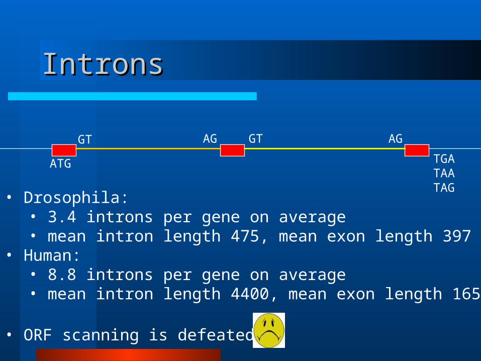
IntronsIntrons

GT GTAG AG

ATG TGATAATAG

• Drosophila:• 3.4 introns per gene on average• mean intron length 475, mean exon length 397

• Human:• 8.8 introns per gene on average• mean intron length 4400, mean exon length 165

• ORF scanning is defeated

SplicingSplicing

GT GTAG AG

ATG TGATAATAG

GT GTAG AG

ATG TGATAATAG

AG

Needles in a HaystackNeedles in a Haystack

Human genome is about 3.2Gbp20,000 – 25,000 genes78% intergenic, 20% introns, 2% coding

Gotta Find ‘Em AllGotta Find ‘Em All

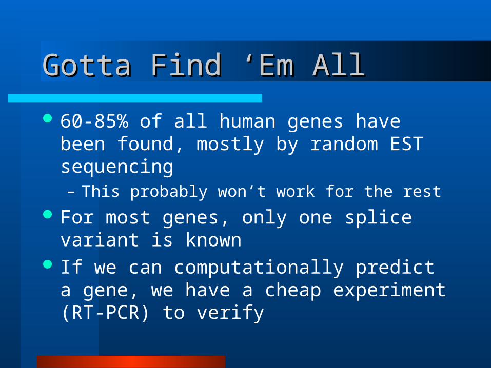
60-85% of all human genes have been found, mostly by random EST sequencing– This probably won’t work for the rest

For most genes, only one splice variant is known

If we can computationally predict a gene, we have a cheap experiment (RT-PCR) to verify

Looking For CluesLooking For Clues

Signals used by the cell– 99% of introns begin with GT, end with AG– 0.8% of introns begin with GC, end with AG– Gene begins with ATG– Gene ends with TAG, TAA, or TGA

Other properties of genes– Exons have characteristic lengths– Base composition of exons is characteristic due to genetic

code– Exons tend to be conserved between species

• Pattern of conservation is three-periodic

Three-PeriodicityThree-Periodicity

Most amino acids can be coded for by more than one DNA triplet (codon)

Usually, the degeneracy is in the last position

Human CCTGTT (Proline, Valine)Mouse CCAGTC (Proline, Valine)Rat CCAGTC (Proline, Valine)Dog CCGGTA (Proline, Valine)Chicken CCCGTG (Proline, Valine)

Hidden Markov ModelsHidden Markov Models

The de facto standard for gene prediction Probabilistic finite state machine Transition to a state, emit a character, transition to a

new state– Many independence assumptions

CDS NC

ACG )|()|()|()|()|()( CDSGPNCCDSPNCCPNCNCPNCAPNCP

HMMs For Gene PredictionHMMs For Gene Prediction

Generative model– Define P(X, Y) as a product of many independent

termsP(ACG) = P(start in noncoding) *P(noncoding emits A) *P(noncoding transitions to noncoding) *P(noncoding emits C) *P(noncoding transitions to coding) *P(coding emits A)• Terms are of the forms P(yi | yi-1) and P(xi | yi)

– Trained by collecting counts

HMMs For Gene PredictionHMMs For Gene Prediction

To predict genes given a sequence X, calculateargmaxY P(Y | X) = argmaxY P(X, Y) / P(X) =

argmaxY P(X, Y)

Generalized Hidden Markov Generalized Hidden Markov ModelsModels Like a HMM, but state durations are explicit Transition to a state, pick a duration d, emit d

characters, transition to a new state Dynamic programming algorithm complexity

goes from O(N2L) to O(N2LK)– K is the maximum state duration– Not so bad in practice

Predicting Genes With HMMsPredicting Genes With HMMs

Given a sequence, we can calculate the most likely annotation

InternalExon

Intron

Inter-genic

FinalExon

InitialExon

SingleExon

GGTGAGGTGACCAAGAACGTGTTGACAGTAGGTGAGGTGACCAAGAACGTGTTGACAGTAGGTGAGGTGACCAAGAACGTGTTGACAGTAGGTGAGGTGACCAAGAACGTGTTGACAGTA

The Past: GENSCANThe Past: GENSCAN

Chris Burge, Stanford, 1997Before the Human Genome Project

– No alignments available– People still thought there were 100,000

human genes

The GENSCAN ModelThe GENSCAN Model

The GENSCAN ModelThe GENSCAN Model

Output probabilities for NC and CDS depend on previous 5 bases (5th-order)– P(Xi | Xi-1, Xi-2, Xi-3, Xi-4, Xi-5)

Each CDS frame has its own model Special 2nd-order positional models for start

codon, stop codon, and acceptor site Even fancier model for donor sites

– Maximal dependence decomposition (MDD)– Long-range dependencies

Separate model for different isochores

GENSCAN PerformanceGENSCAN Performance

First program to do well on realistic sequences– Multiple genes in both orientations

Pretty good sensitivity, poor specificity– 70% exon Sn, 40% exon Sp

Not enough exons per geneWas the best gene predictor for about 4

years

Comparative Gene PredictionComparative Gene Prediction

ExonIntron

ExonIntron

-3 -2 -1 +1 +2 +3

Human A A G G T G

-3 -2 -1 +1 +2 +3

Human A A G G T G

Mouse A A G G T G Mouse A A T G T G

Chicken A A G G T G Chicken A A _ A C G

A B

The Recent Past: TWINSCANThe Recent Past: TWINSCAN

Korf, Flicek, Duan, Brent, Washington University in St. Louis, 2001

Uses an informant sequence to help predict genes– For human, informant is normally mouse

Informant sequence consists of three characters– Match: |– Mismatch: :– Unaligned: .

Informant sequence assumed independent of target sequence

The TWINSCAN ModelThe TWINSCAN Model

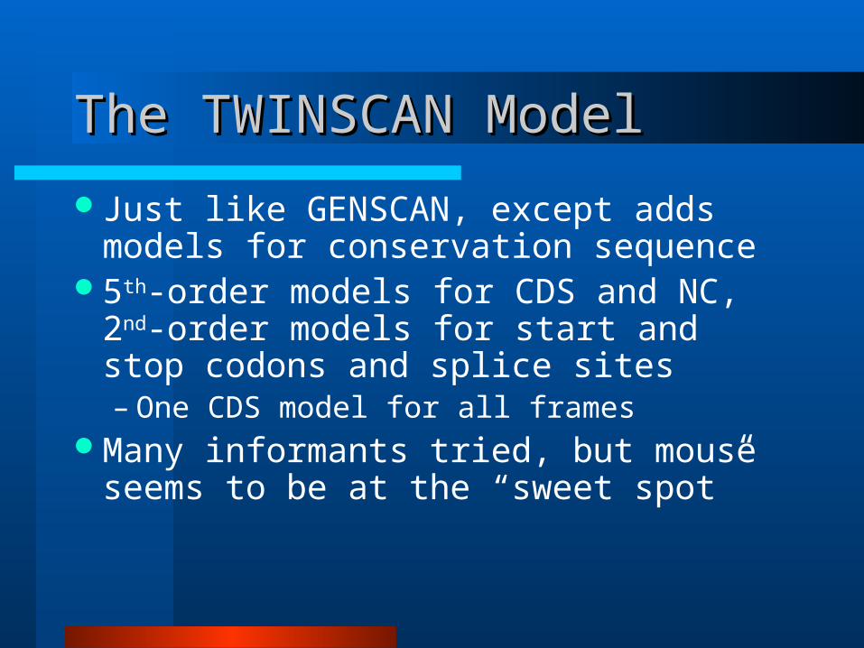
Just like GENSCAN, except adds models for conservation sequence

5th-order models for CDS and NC, 2nd-order models for start and stop codons and splice sites– One CDS model for all frames

Many informants tried, but mouse seems to be at the “sweet spot”

TWINSCAN PerformanceTWINSCAN Performance

Slightly more sensitive than GENSCAN, much more specific– Exon sensitivity/specificity about 75%

Much better at the gene level– Most genes are mostly right, about 25%

exactly rightWas the best gene predictor for about 4

years

The Present: N-SCANThe Present: N-SCAN

Gross and Brent, Washington University in St. Louis, 2005

If one informant sequence is good, let’s try more!

Also several other improvements on TWINSCAN

N-SCAN ImprovementsN-SCAN Improvements

Multiple informants

Richer models of sequence evolution

Frame-specific CDS conservation model

Conserved noncoding sequence model

5’ UTR structure model

GENSCAN

TWINSCAN

N-SCAN

HMM OutputsHMM Outputs

Target GGTGAGGTGACCAAGAACGTGTTGACAGTA

Target GGTGAGGTGACCAAGAACGTGTTGACAGTAConservation |||:||:||:|||||:||||||||......sequence

Target GGTGAGGTGACCAAGAACGTGTTGACAGTAInformant1 GGTCAGC___CCAAGAACGTGTAG......Informant2 GATCAGC___CCAAGAACGTGTAG......Informant3 GGTGAGCTGACCAAGATCGTGTTGACACAA.

..

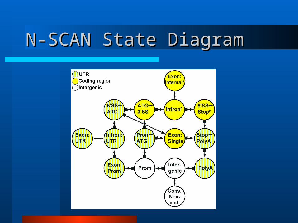
N-SCAN State DiagramN-SCAN State Diagram

Two-Component Output Two-Component Output DistributionsDistributions

Target sequence model

Phylogenetic model for informants

Product gives the probability of a multiple alignment column

),...,,...,|( 1 oiioiii TTP III

),...,|( 1 oiii TTTP

),...,,,...,|,( 11 oiioiiii TTTP III

Phylogenetic Bayesian Network Phylogenetic Bayesian Network ModelsModels

)|()|()|(

)|()|()|()(),,,,,,(

3323

21211321

ARPAMPAAP

AHPAAPACPAPAAARMCHP

)|()|()|(

)|()|()|()(),,,,,,(

331

23212321

ARPAMPACP

AAPAAPHAPHPAAARMCHP

Graph TransformationGraph Transformation

InferenceInference

Slightly-modified version of Felsenstein’s algorithm

At each of the O(N) nodes, we calculate 6o+1 summations over 6o+1 values

Total time complexity is O(N • 62(o+1))

TrainingTraining

Simple with labeled multiple alignment of all sequences

Can use known genes as a labeling

Don’t know ancestral genome sequences– Treat them as missing data and use EM

CPD ParameterizationsCPD Parameterizations Each Bayesian network of order o has

(2N-1)(6o+1)(6o+1-1) free parameters

We can reduce this number by restricting the form of the CPDs

Partially reversible models– Relative frequency of DNA k-mers remains constant as sequence

evolves– Gaps and unaligned regions introduced over time

N-SCAN Phylogenetic Models N-SCAN Phylogenetic Models vs. Traditional Phylogenetic vs. Traditional Phylogenetic ModelsModels

Root (target) node is observed

– Can use existing single-sequence models

– Can use higher-order models

– Can estimate target sequence model optimally

No assumption of homogeneous substitution process

– Gaps and unaligned regions can be treated naturally

– Robust against

• Function-changing mutation

• Alignment error

• Sequencing error

– The price is many more parameters

N-SCAN Phylogenetic Models N-SCAN Phylogenetic Models vs. Traditional Phylogenetic vs. Traditional Phylogenetic ModelsModels

Conservation Score CoefficientConservation Score Coefficient

N-SCAN uses log-likelihood scores internally. The score of a position i under state S is

Values of k between 0.3 and 0.6 result in the best performance– Performance is roughly constant in this range

)|(

)|(log

)|(

)|(log

NullP

SPk

NullTP

STP

i

i

i

i

I

I

Whole-Genome Human Gene Whole-Genome Human Gene PredictionPredictionAnnotations used were cleaned

RefSeqs– 16,259 genes

– 20,837 transcripts

N-SCAN used human, mouse, rat, chicken alignment

Exact Exon AccuracyExact Exon Accuracy

0.2

0.3

0.4

0.5

0.6

0.7

0.8

0.9

Exon Sn Exon Sp

GENSCAN EXONIPHY SGP2 TWINSCAN 2.0 N-SCAN

Exact Gene AccuracyExact Gene Accuracy

0

0.1

0.2

0.3

0.4

0.5

Gene Sn Gene Sp

GENSCAN SGP2 TWINSCAN 2.0 N-SCAN

Intron Sensitivity By LengthIntron Sensitivity By Length

0

0.2

0.4

0.6

0.8

1

0-10

10-2

0

20-3

0

30-4

0

40-5

0

50-6

0

60-7

0

70-8

0

80-9

0

90-1

00Length (Kb)

N-SCANSGP2GENSCANTWINSCAN

Human Informant EffectivenessHuman Informant Effectiveness

00.10.20.30.40.50.60.70.80.9

Gene Sn Gene Sp Exon Sn Exon Sp

Chicken Rat Mouse All

Drosophila Drosophila Informant EffectivenessInformant Effectiveness

0.3

0.4

0.5

0.6

0.7

0.8

0.9

Gene Sn Gene Sp Exon Sn Exon Sp

A. gambiae D. yakuba D. pseudoobscura All

The Future(?): CONTRASTThe Future(?): CONTRAST

New gene predictor currently in the works

Based not on a generalized HMM, but a semi-Markov conditional random field (SCRF)

HMMs For Gene PredictionHMMs For Gene Prediction

Generative model– Define P(X, Y) as a product of many independent

termsP(ACG) = P(start in noncoding) *P(noncoding emits A) *P(noncoding transitions to noncoding) *P(noncoding emits C) *P(noncoding transitions to coding) *P(coding emits A)• Terms are of the forms P(yi | yi-1) and P(xi | yi)

– Trained by collecting counts

HMMs For Gene PredictionHMMs For Gene Prediction

To predict genes given a sequence X, calculateargmaxY P(Y | X) = argmaxY P(X, Y) / P(X) =

argmaxY P(X, Y) Advantage: simplicity

– Extremely fast training, efficient inference Disadvantage: simplicity

– Makes many unwarranted independence assumptions

– Inaccurate model will get us into trouble

When HMMs Go WrongWhen HMMs Go Wrong

Normal HMM training optimizes wrong function– We use P(Y | X) for prediction, but we’re

optimizing P(X, Y) = P(Y | X) P(X)– This means we may prefer parameters that

lead to worse predictions if they assign a higher probability to the sequence

When HMMs Go WrongWhen HMMs Go Wrong

NCA 3%B 2%C 95%

CDSA 49%B 49%C 2%

NCA 3%B 2%C 95%

CDSA 3%B 95%C 2%

NNCA 2%B 2%C 96%

CNSA 96%B 2%C 2%

CDSA 49%B 49%C 2%

A = Conserved tripletB = Synonymous substitutionC = Nonsynonymous substitution

…CCCCCCCCCCCCCAAAAAAAAAACCCC…CCCCCCCBBABAAABBABBABCC…

Can We Fix It?Can We Fix It?

Directly optimize

No closed form solution– But function and gradient can be calculated

efficiently using DP If we’re going to numerically optimize anyway,

might as well switch to a more expressive model

),(

),()|(

YXP

YXPXYP

Y

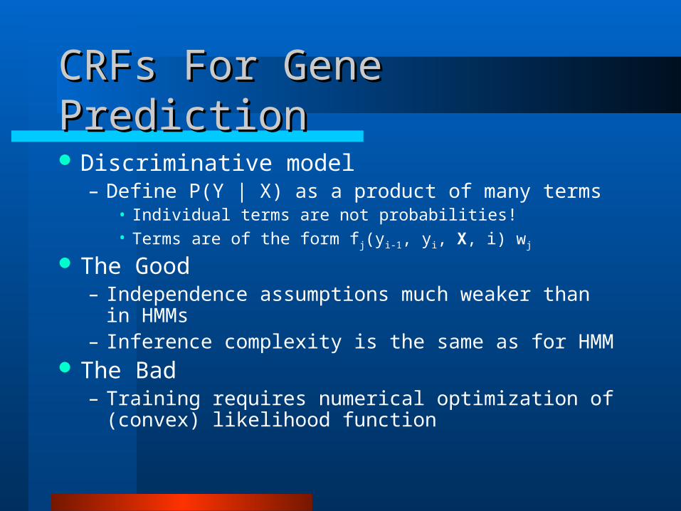
CRFs For Gene PredictionCRFs For Gene Prediction

Discriminative model– Define P(Y | X) as a product of many terms

• Individual terms are not probabilities!• Terms are of the form fj(yi-1, yi, X, i) wj

The Good– Independence assumptions much weaker than in

HMMs– Inference complexity is the same as for HMM

The Bad– Training requires numerical optimization of (convex)

likelihood function

The MathThe Math

ji

iijj wiXyyfYXF ),,,(),( 1

jj YXF

XZXYP ),(exp

)(

1)|(

Y jj YXFXZ ),(exp)(

CRFs

i

iiiiba aybyPaybyYXT )|(log],[1),( 11,

i

iiiisa syaxPaxsyYXE )|(log],[1),(,

HMMs

sasa

baba YXEYXTYXP

,,

,, ),(),(exp),(

HMMs vs. CRFsHMMs vs. CRFs

y1

x1

y2

x2

y3

x3

y4

x4

y5

x5

y6

x6

…HMM

y1

x1

y2

x2

y3

x3

y4

x4

y5

x5

y6

x6

…CRF

HMMs vs. CRFsHMMs vs. CRFs

HMM-style “features”– Last state is exon, current state is intron– Current state is exon, current sequence character is “C”

CRF-style features– Current state is exon, CG percent in 100Kbp window is

between 40% and 50%, at least one CpG island predicted within 10Kbp

– Current state is exon, 3 unspliced ESTs with at least 95% identity aligned near current position

– Current state is exon, 1 spliced EST with at least 95% identity aligned near current position

Semi-Markov CRFsSemi-Markov CRFs

Semi-Markov CRFs are to CRFs as generalized HMMs (or semi-HMMs) are to HMMs

Instead of assigning labels to each position, assign labels to segments

Features are f(yi-1, yi, X, i, j)

Future DirectionsFuture Directions

SVM-based splice site models that use alignment information– Splice site models in current gene

predictors are pretty primitiveAlternative splicing!

– Not yet handled well– Very poor experimental coverage of

transcriptome