This paper presents preliminary findings and is being distributed to economists

and other interested readers solely to stimulate discussion and elicit comments.

The views expressed in this paper are those of the authors and do not necessarily

reflect the position of the Federal Reserve Bank of New York or the Federal

Reserve System. Any errors or omissions are the responsibility of the authors.

Federal Reserve Bank of New York

Staff Reports

Gender and Dynamic Agency: Theory and

Evidence on the Compensation of Top

Executives

Stefania Albanesi

Claudia Olivetti

María José Prados

Staff Report No. 718

March 2015

Gender and Dynamic Agency: Theory and Evidence on the Compensation of Top

Executives

Stefania Albanesi, Claudia Olivetti, and María José Prados

Federal Reserve Bank of New York Staff Reports, no. 718

March 2015

JEL classification: G3, J16, J31, J33, M12

Abstract

We document three new facts about gender differences in executive compensation. First, female

executives receive a lower share of incentive pay in total compensation relative to males. This

difference accounts for 93 percent of the gender gap in total pay. Second, the compensation of

female executives displays lower pay-performance sensitivity. A $1 million increase in firm value

generates a $17,150 increase in firm-specific wealth for male executives and a $1,670 increase for

females. Third, female executives are more exposed to bad firm performance and less exposed to

good firm performance relative to male executives. We find no link between firm performance

and the gender of top executives. We discuss evidence on differences in preferences and the cost

of managerial effort by gender and examine the resulting predictions for the structure of

compensation. We consider two paradigms for the pay-setting process, the efficient contracting

model and the “managerial power" or skimming view. The efficient contracting model can

explain the first two facts. Only the skimming view is consistent with the third fact. This suggests

that the gender differentials in executive compensation may be inefficient.

Key words: gender differences in executive pay, incentive pay, pay-performance sensitivity

_________________

Corresponding author: Albanesi: Federal Reserve Bank of New York (e-mail:

stefania.albanesi@ny.frb.org). Olivetti: Boston University and NBER (e-mail: olivetti@bu.edu).

Prados: University of Southern California (e-mail: prados@usc.edu). The authors thank

Konstantinos Tatsiramos, Solomon Polachek, and an anonymous referee for their constructive

feedback. They are grateful to Alex Edmans, Carola Frydman, Martin Lettau, Karen Selody, and

seminar participants at the University of California Santa Barbara, Wharton, and the NBER for

helpful comments and suggestions. They also thank Mikhail Pyatigorsky for excellent research

assistance. This research was supported in part by the National Science Foundation under Grant

SES0820135 (Albanesi) and Grant SES0820127 (Olivetti). The views expressed in this paper are

those of the authors and do not necessarily reflect the position of the Federal Reserve Bank of

New York or the Federal Reserve System.

1 Introduction

We document three new facts about gender differences in the structure of executive compensation.

First, female executives receive a lower share of incentive pay in total compensation relative to

males. This difference accounts for 93% of the gender differences in total flow compensation. Sec-

ond, the compensation of female executives displays a lower pay-performance sensitivity relative

to males. A $1 million dollar increase in firm value generates a $17,150 increase in firm specific

wealth for male executives and a $1,670 increase for females. Third, female executives’ pay is

more exposed to bad firm performance and less exposed to good firm performance than for males.

A 1% increase in firm value generates a 13% rise in firm specific wealth for female executives, and

a 44% rise for male executives, while a 1% decline in firm value generates a 63% decline in firm

specific wealth for female executives and only a 33% decline for male executives. We also show

that there is no link between firm performance and the gender of top executives. These results

are based on ExecuComp, Standard&Poor’s database on executive compensation, and control for

the fact that women are younger and tend to hold lower ranked titles.

What drives these differences in the structure of compensation by gender? To examine this

question, we discuss evidence on gender differences in preferences and the cost of managerial effort

and examine the resulting predictions for the structure of compensation based on two models of

the firm-executive relationship.

Our analysis builds on an extensive literature on gender differences in attributes relevant for

the executive labor market. First, surveys of professionals and managers point to the existence

of a pervasive set of barriers to career advancement for women. These include exclusion from

informal networks, gender based stereotyping, lack of mentors and role models and asymmetric

allocation of household responsibilities (Catalyst, 2004a). The evidence of gender asymmetries in

the personal cost of career investments in relation to marriage and parenthood is also substantial.

High earning professional and executive women are less likely than men in similar circumstances

to be married or have children, but they bear a larger fraction of household responsibilities if

married (Hewlett, 2002). Finally, there is substantial evidence of gender differences in preferences

from field and experimental studies. We concentrate on three attributes that appear particularly

relevant for executives: ability to perform in competitive environments, propensity to compete

and initiate negotiations, and risk aversion, all of which seem to be substantially lower for women.1

To explore the impact of these gender differences on executive compensation, we consider two

paradigms, the classic agency model of executive compensation and the “managerial power” or

skimming view. According to the agency model (Holmstrom, 1979, and Jensen and Murphy,

1990), shareholders set executive’s pay to maximize the surplus from their relationship. Private

information over the executive’s effort generates moral hazard, which requires pay to be sensitive to

firm performance to insure incentive compatibility. Equity based pay or explicit bonus programs

can be used to obtain this effect. Under this paradigm, the structure, as well as the level, of

executive compensation will reflect actual or perceived attributes of the executive, such as their

impact on firm performance, their cost of effort and risk aversion.

1We review this evidence in more detail and discuss its limitations in Section 3

1

The managerial power or skimming view (Bertrand and Mullainathan, 2001, and Bebchuk

and Fried, 2003) is based on the notion that the members of the board of directors, who are

typically responsible for setting executive pay, cannot be expected to make decisions to maximize

shareholder value. The incentive to be re-elected, informal networks linking them to CEOs,

cognitive dissonance, and ratcheting all imply that executives can exert significant power over

their own compensation. This has implications for the structure, as well as the level of pay.

Executive compensation will rely more on forms of pay that are less transparent, and will be

more sensitive to good firm performance than to adverse performance. These patterns should be

more prevalent for executives that are more entrenched.

If we posit that gender differences in performance in competitive environments, propensity to

compete and to initiate negotiation and weight of household responsibilities reduce the impact of

female executive on firm performance and increase their cost of effort, the efficient contracting

model can explain the fact that female executives have a lower share of incentive pay in total

compensation and display lower pay-performance sensitivity. These patterns are also consistent

with the evidence on risk aversion by gender. However, the efficient contracting model cannot

explain why female executives are more exposed to adverse firm performance. The skimming

view is consistent with this fact, since female executives, who are younger, have lower tenure

and are limited in accessing informal networks, are likely to be less entrenched than their male

counterparts.

Our results suggest that the gender differences in the structure and level of compensation are

not efficient. The gender differentials in the level of compensation are mostly accounted for by

those in the share of incentive pay. Moreover, female executives’ greater exposure to risk can

be linked to equity based compensation. The implications of these findings extend beyond the

executive labor market. Lemieux, MacLeod and Parent (2009) document a rise in the fraction of

U.S. jobs explicitly linking pay to performance since the late 1970s. They show that this trend

can explain a sizable fraction of the growth in male wage dispersion, especially at the top-end.

Hall and Murphy (2003) discuss the rise in equity based programs for employees at all levels since

the early 1990s. Albanesi and Olivetti (2009) find that gender earnings differentials are greatest

in occupations and industries with higher incidence of incentive pay.

The failure of the efficient contracting paradigm to explain the three facts on gender differences

in the structure of executive compensation points to the possibility of distortions in the link be-

tween pay and performance that may influence a broader set of workers as incentive pay schemes

become increasingly important. To the extent that performance pay amplifies earnings differ-

entials resulting from effective or perceived differences in attributes across workers, if designed

incorrectly, it exacerbates inequality and discrimination and can severely distort the allocation of

resources. Our analysis suggest that performance pay schemes should be held to closer scrutiny

and raises a note of concern for the standing of professional women in the labor market as incentive

pay becomes more prevalent.

The paper is organized as follows. We discuss the three facts on gender differentials in the

structure of compensation in Section 2. Section 3 reviews the evidence on gender differences in

preferences and barriers to career advancement. We describe the efficient contracting model of

2

executive compensation and the skimming view in Section 4 and evaluate their predictions against

the evidence on gender differences in preferences and the structure of executive compensation.

Section 5 discusses some open questions.

2 Evidence on the Compensation of Top Executives

It is well known that there are significant gender differences in the level of compensation for top

executives. Bertrand and Hallock (2001) are the first to systematically document this gender

differentials based on ExecuComp data. They show that the gender differential can, for the most

part, be accounted for by the size and industry distribution of female executives, in particular,

the fact that women are represented in smaller firms and that they are less likely to hold the

title of CEO (or other top ranked titles). The fact that female top executives are younger and

have fewer years of tenure contributes to explain most of the remaining gender differential in total

compensation. Additional studies by Bell (2005), and Elkinaway and Stater (2011) further confirm

these results. By contrast Gayle, Golan and Miller (2012) find that controlling for executive rank

and background, women earn higher compensation than men and are promoted more quickly,

but experience more income uncertainty. They also find that the unconditional gender pay gap

and job-rank differences are primarily attributable to female executives exiting the occupation at

higher rates than men.

The contribution of our paper is to use ExecuComp data for 1992 to 2005 to document three

new facts about gender differences in the structure of executive compensation.

Fact 1: Female executives receive lower levels of incentive pay relative to males. For the yearly flow

of compensation, we find a residual female-male gap of -6 log points. The gap is much larger

for measures of firm specific wealth, ranging from -10 to -30 log points.

Fact 2: The compensation of female executives displays a lower pay-performance sensitivity relative

to males. A $1 million increase in firm value generates a $17,150 increase in firm specific

wealth for male executives and a $1,670 increase for females.

Fact 3: The compensation of female executives is more exposed to declines in firm value and less

exposed to increases in firm value than that of males. While a 1% rise in firm value is

associated with a 13% and 44% rise in firm specific wealth for female and male executives,

respectively, a 1% decline in firm value is associated with a 63% decline in firm specific

wealth for female executives and a 33% decline for males.

Finally, we show that there is no link between standard measures of firm performance and

female representation in the team of top executives. It is, therefore, unlikely that we are only

capturing differences in performance by female-led firms.

2.1 Data and sample selection

Our analysis is based on data from Standard & Poor’s ExecuComp. This data set collects in-

formation on the compensation of top executives in firms belonging to the S&P 500, the S&P

3

Midcap 400 and the S&P SmallCap 600. Firms report compensation data for the top 1 to 15

executives, depending on size. Approximately 70% of firms report information for 4 to 9 top

executives, around 45% of the firms in the sample report information for 5 to 6 executives. To

minimize potential problems due to the variation in the number of executives across firms we focus

on the top-5 executives as defined by title. Specifically, our sample only includes Chair/CEOs,

Vice Chairs, Presidents, CFOs and COOs.

Although the ExecuComp data set runs from 1992 to the present, we restrict our sample to the

period 1992-2005. This is because of the disclosure reform passed in 2006 which changed reporting

of several form of incentive pay thus making pre and post 2006 data not directly comparable.2 The

resulting sample with non-missing information on the relevant variables includes 40,704 executives

of which 1,312 are females (that is, women are only 3.2% of our sample). Table 10 in the Data

Appendix presents summary statistics on the composition of this sample. Female executives are

on average younger than male executives (48 and 54 years of age, respectively) and have lower

average firm tenure (8 and 14 years, respectively). Women tend to be under-represented at higher

ranks. The percentage of female CEOs is 1.4% over the entire period (growing from a mere

0.002% in 1992 to 2.2% in 2005). Women make 6% of all CFOs, 4.3% of all Vice Chairs, 4.5% of

all Presidents and 3.5% of all COOs.

The information on age and tenure is only available for a sub-sample of executives. Controlling

for age reduces the sample by 28% and, unfortunately, we loose a disproportionate amount of

female executives. The share of female in this case drops to 2.3% of sample.3

2.2 Main Variables

Most of our analysis focuses on three alternative ways to measure total executive compensation.

The first and most commonly used measure is TDC1. This is a flow measure that includes

salary as well as an array of “incentive pay” components that are perceived to be linked to firm

performance. In ExecuComp, these correspond to Bonus, Stocks Granted and Stock Options.

Bonus typically includes discretionary bonus as well as cash payments resulting from performance

based bonus programs. Stocks Granted and Stock Options are a measure of the equity component

of incentive pay.4

One important feature of incentive pay is that it leads to the build up of firm specific wealth,

from previous years’ flow of stock options and stock grants. Small fluctuations in a company’s

stock value may lead to large swings in the value of outstanding stock options and stock grants,

typically larger than flow components of compensation. For this reason, we consider two additional

measures of compensation that capture the executive’s stock of firms specific wealth. Specifically,

2The change in reporting rules in 2006 resulted in a change in the definition and availability of ExecuCompvariables. So for the post-2006 period most items under the 2006 definition are not fully comparable to those underthe 1992 definition, which we use in our analysis. See Data Appendix for further details on sample selection.

3When controlling for non-missing age, the male executives sample declines by 27% while the female executivesample declines by half, see table 10 in the Data Appendix. The loss is even more severe for tenure, in this case weloose 62% of all the observations. Thus, we do not use this control in our analysis.

4Bebchuk and Fried (2003) have argued that stock options programs are often structured in a way that doesnot make them sensitive to performance. We explore this issue in Section 2.4.

4

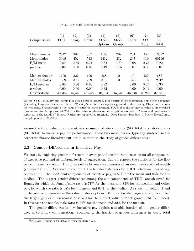
Table 1: Gender Differences in Average and Median Pay

(1) (2) (3) (4) (5) (6) (7) (8)Compensation TDC1 Salary Bonus Stock Stock Other SO SG

Options Grants Total Total

Mean females 2542 382 367 1186 287 201 457 13572Mean males 3099 452 518 1412 332 297 610 60796F/M mean 0.82 0.85 0.71 0.84 0.87 0.68 0.75 0.22p-value 0.02 0.00 0.00 0.19 0.65 0.01 0.00 0.07

Median females 1199 322 190 288 0 19 187 686Median males 1389 376 229 313 0 32 215 2312F/M median 0.86 0.86 0.83 0.92 0.60 0.87 0.30p-value 0.00 0.00 0.00 0.32 0.00 0.01 0.00

Observations 40,704 45,548 45,548 40,704 45,548 45,548 40,222 37,581

Notes: TDC1 is salary and bonus plus stock options granted, plus restricted stock granted, plus other payments(including long-term incentive plans), StockOptions is stock options granted, valued using Black and Scholesmethodology, StockGrants is the value of restricted stock granted, SOTotal is the estimated value of unexercisedplus unexercisable options, SGTotal is the value of shares owned - options excluded. Means and medians arereported in thousands of dollars. Ratios are reported as fractions. Data Source: Standard & Poor’s ExecuComp.Sample period: 1992-2005.

we use the total value of an executive’s accumulated stock options (SO Total) and stock grants

(SG Total) to measure pay for performance. These two measures are typically analyzed in the

corporate finance literature but not in relation to the study of gender differentials.5

2.3 Gender Differences in Incentive Pay

We start by exploring gender differences in average and median compensation for all components

of executive pay and at different levels of aggregation. Table 1 reports the statistics for the flow

pay components (column 1 to 6) as well as for our two measures of an executive’s stock of wealth

(column 7 and 8). As shown in column 1, the female/male ratio for TDC1, which includes salary,

bonus and all the additional components of incentive pay, is 82% for the mean and 86% for the

median. The biggest gender differences among the sub-components of TDC1 are observed for

Bonus, for which the female/male ratio is 71% for the mean and 83% for the median, and Other

pay, for which the ratio is 68% for the mean and 60% for the median. As shown in column 7 and

8, the gender differential in the value of stock options (SO Total) is also large and significant but

the largest gender differential is observed for the market value of stock grants held (SG Total).

In this case the female/male ratio is 22% for the mean and 30% for the median.

The gender differences in flow incentive pay explain a sizable fraction of the gender differ-

ence in total flow compensation. Specifically, the fraction of gender differences in yearly total

5See Data Appendix for detailed variable definitions.

5

compensation explained by differences in the flow of incentive pay, that is

Incentive Paym − Incentive PayfTCm − TCf

,

is 93%. Gender differences in stock options grants alone account for 41% of the gender difference

in flow compensation. However, stock grants play a much larger role for gender differences in firm

specific wealth, as they account for 99.7% of the gender difference in firm specific wealth.

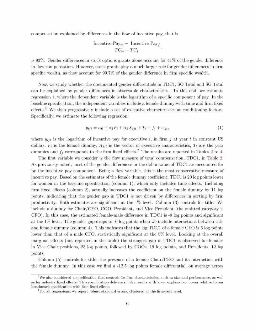
Next we study whether the documented gender differentials in TDC1, SO Total and SG Total

can be explained by gender differences in observable characteristics. To this end, we estimate

regression 1, where the dependent variable is the logarithm of a specific component of pay. In the

baseline specification, the independent variables include a female dummy with time and firm fixed

effects.6 We then progressively include a set of executive characteristics as conditioning factors.

Specifically, we estimate the following regression:

yijt = α0 + α1Fi + α2Xijt + Tt + fj + εijt, (1)

where yijt is the logarithm of incentive pay for executive i, in firm j at year t in constant US

dollars, Fi is the female dummy, Xijt is the vector of executive characteristics, Tt are the year

dummies and fj corresponds to the firm fixed effects.7 The results are reported in Tables 2 to 4.

The first variable we consider is the flow measure of total compensation, TDC1, in Table 2.

As previously noted, most of the gender differences in the dollar value of TDC1 are accounted for

by the incentive pay component. Being a flow variable, this is the most conservative measure of

incentive pay. Based on the estimates of the female dummy coefficient, TDC1 is 20 log points lower

for women in the baseline specification (column 1), which only includes time effects. Including

firm fixed effects (column 2), actually increases the coefficient on the female dummy by 11 log

points, indicating that the gender gap in TDC1 is not driven by differences in sorting by firm

productivity. Both estimates are significant at the 1% level. Column (3) controls for title. We

include a dummy for Chair/CEO, COO, President, and Vice President (the omitted category is

CFO). In this case, the estimated female-male difference in TDC1 is -9 log points and significant

at the 1% level. The gender gap drops to -6 log points when we include interactions between title

and female dummy (column 4). This indicates that the log TDC1 of a female CFO is 6 log points

lower than that of a male CFO, statistically significant at the 5% level. Looking at the overall

marginal effects (not reported in the table) the strongest gap in TDC1 is observed for females

in Vice Chair positions, 23 log points, followed by COOs, 19 log points, and Presidents, 12 log

points.

Column (5) controls for title, the presence of a female Chair/CEO and its interaction with

the female dummy. In this case we find a -12.5 log points female differential, on average across

6We also considered a specification that controls for firm characteristics, such as size and performance, as wellas for industry fixed effects. This specification delivers similar results with lower explanatory power relative to ourbenchmark specification with firm fixed effects.

7For all regressions, we report robust standard errors, clustered at the firm-year level.

6

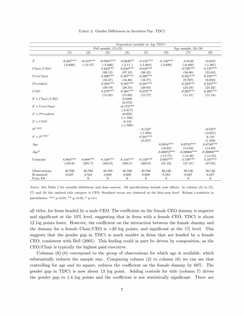
Table 2: Gender Differences in Incentive Pay. TDC1

Dependent variable is: log TDC1Full sample, (1)-(5) Age sample, (6)-(8)

(1) (2) (3) (4) (5) (6) (7) (8)

F -0.207*** -0.310*** -0.0931*** -0.0630** -0.125*** -0.126*** -0.0140 -0.0427(-6.699) (-13.47) (-4.566) (-2.11 ) (-5.884) (-3.698) (-0.460) (-1.361)

Chair/CEO 0.823*** 0.824*** 0.819*** 0.739*** 0.737***(99.12) (97.35) (98.22) (56.06) (55.63)

V iceChair 0.290*** 0.297*** 0.288*** 0.201*** 0.199***(16.87) (16.86) (16.77) (9.707) (9.659)

President 0.282*** 0.285*** 0.281*** 0.333*** 0.332***(29.19) (28.54) (29.03) (24.34) (24.22)

COO 0.279*** 0.285*** 0.278*** 0.263*** 0.262***(15.82) (15.69) (15.77) (11.21) (11.18)

F × Chair/CEO 0.0406(0.573)

F × V iceChair -0.172***(-2.817)

F × President -0.0561(-1.196)

F × COO -0.131(-1.599)

FCEO -0.122* -0.0477(-1.950) (-0.651)

F × FCEO 0.201*** 0.116(3.257) (1.459)

Age 0.0916*** 0.0752*** 0.0749***(16.63) (14.03) (14.00)

Age2 -0.00072*** -0.00068*** -0.00068***(-14.74) (-14.46) (-14.42)

Constant 6.904*** 6.698*** 6.146*** 6.144*** 6.150*** 3.956*** 4.158*** 4.167***(183.8) (291.7) (264.0) (263.5) (263.9) (25.42) (27.51) (27.62)

Observations 40,700 40,700 40,700 40,700 40,700 30,136 30,136 30,136R-squared 0.027 0.524 0.608 0.608 0.608 0.583 0.627 0.627Firm FE X X X X X X X

Notes: See Table 1 for variable definitions and data sources. All specifications include year effects. In column (3) to (5),

(7) and (8) the omitted title category is CFO. Standard errors are clustered at the firm-year level. Robust t-statistics in

parentheses. *** p<0.01, ** p<0.05, * p<0.1

all titles, for firms headed by a male CEO. The coefficient on the female CEO dummy is negative

and significant at the 10% level, suggesting that in firms with a female CEO, TDC1 is about

12 log points lower. However, the coefficient on the interaction between the female dummy and

the dummy for a female Chair/CEO is +20 log points, and significant at the 1% level. This

suggests that the gender gap in TDC1 is much smaller in firms that are headed by a female

CEO, consistent with Bell (2005). This finding could in part be driven by composition, as the

CEO/Chair is typically the highest paid executive.

Columns (6)-(8) correspond to the group of observations for which age is available, which

substantially reduces the sample size. Comparing column (2) to column (6) we can see that

controlling for age and its square, reduces the coefficient on the female dummy by 60%. The

gender gap in TDC1 is now about 13 log point. Adding controls for title (column 7) drives

the gender gap to 1.4 log points and the coefficient is not statistically significant. There are

7

disproportionately fewer female executives in the sample with non-missing age (their share drops

from 3.2% to 2.3%), thus this can at least in part explain the loss of precision in the estimate.

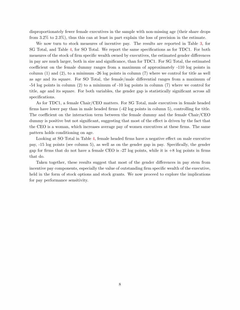
We now turn to stock measures of incentive pay. The results are reported in Table 3, for

SG Total, and Table 4, for SO Total. We report the same specifications as for TDC1. For both

measures of the stock of firm specific wealth owned by executives, the estimated gender differences

in pay are much larger, both in size and significance, than for TDC1. For SG Total, the estimated

coefficient on the female dummy ranges from a maximum of approximately -110 log points in

column (1) and (2), to a minimum -26 log points in column (7) where we control for title as well

as age and its square. For SO Total, the female/male differential ranges from a maximum of

-54 log points in column (2) to a minimum of -10 log points in column (7) where we control for

title, age and its square. For both variables, the gender gap is statistically significant across all

specifications.

As for TDC1, a female Chair/CEO matters. For SG Total, male executives in female headed

firms have lower pay than in male headed firms (-42 log points in column 5), controlling for title.

The coefficient on the interaction term between the female dummy and the female Chair/CEO

dummy is positive but not significant, suggesting that most of the effect is driven by the fact that

the CEO is a woman, which increases average pay of women executives at these firms. The same

pattern holds conditioning on age.

Looking at SO Total in Table 4, female headed firms have a negative effect on male executive

pay, -15 log points (see column 5), as well as on the gender gap in pay. Specifically, the gender

gap for firms that do not have a female CEO is -27 log points, while it is +8 log points in firms

that do.

Taken together, these results suggest that most of the gender differences in pay stem from

incentive pay components, especially the value of outstanding firm specific wealth of the executive,

held in the form of stock options and stock grants. We now proceed to explore the implications

for pay performance sensitivity.

8

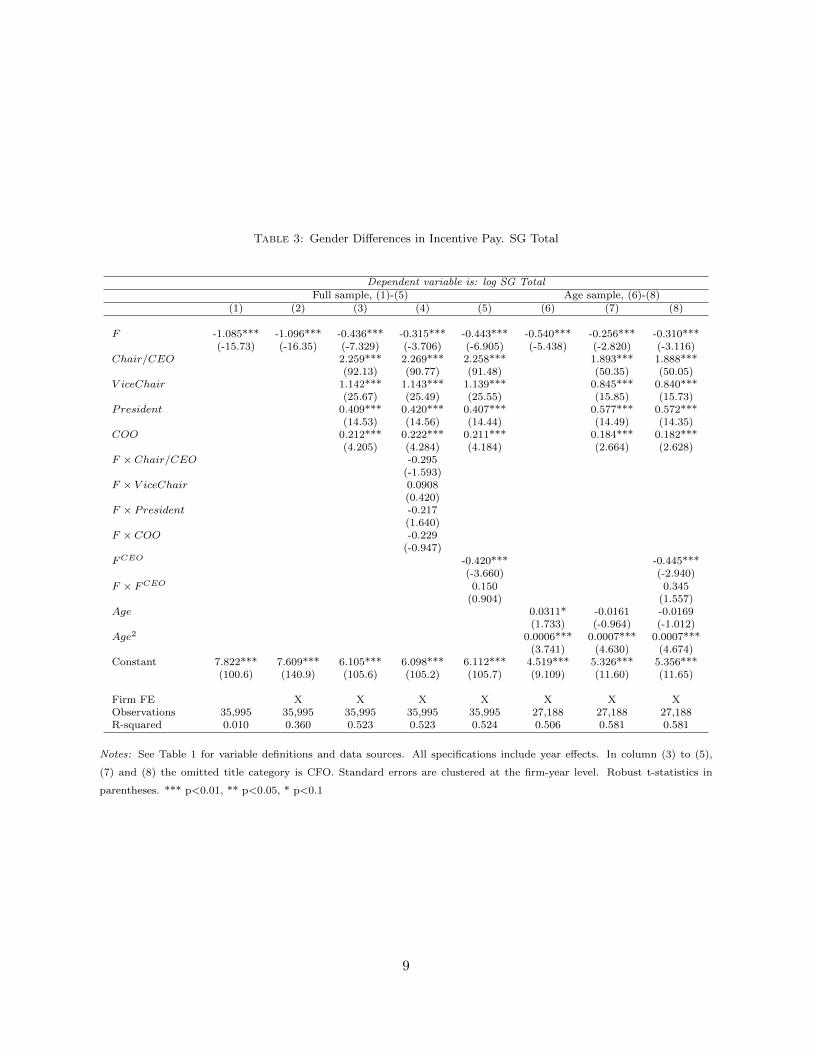
Table 3: Gender Differences in Incentive Pay. SG Total

Dependent variable is: log SG TotalFull sample, (1)-(5) Age sample, (6)-(8)

(1) (2) (3) (4) (5) (6) (7) (8)

F -1.085*** -1.096*** -0.436*** -0.315*** -0.443*** -0.540*** -0.256*** -0.310***(-15.73) (-16.35) (-7.329) (-3.706) (-6.905) (-5.438) (-2.820) (-3.116)

Chair/CEO 2.259*** 2.269*** 2.258*** 1.893*** 1.888***(92.13) (90.77) (91.48) (50.35) (50.05)

V iceChair 1.142*** 1.143*** 1.139*** 0.845*** 0.840***(25.67) (25.49) (25.55) (15.85) (15.73)

President 0.409*** 0.420*** 0.407*** 0.577*** 0.572***(14.53) (14.56) (14.44) (14.49) (14.35)

COO 0.212*** 0.222*** 0.211*** 0.184*** 0.182***(4.205) (4.284) (4.184) (2.664) (2.628)

F × Chair/CEO -0.295(-1.593)

F × V iceChair 0.0908(0.420)

F × President -0.217(1.640)

F × COO -0.229(-0.947)

FCEO -0.420*** -0.445***(-3.660) (-2.940)

F × FCEO 0.150 0.345(0.904) (1.557)

Age 0.0311* -0.0161 -0.0169(1.733) (-0.964) (-1.012)

Age2 0.0006*** 0.0007*** 0.0007***(3.741) (4.630) (4.674)

Constant 7.822*** 7.609*** 6.105*** 6.098*** 6.112*** 4.519*** 5.326*** 5.356***(100.6) (140.9) (105.6) (105.2) (105.7) (9.109) (11.60) (11.65)

Firm FE X X X X X X XObservations 35,995 35,995 35,995 35,995 35,995 27,188 27,188 27,188R-squared 0.010 0.360 0.523 0.523 0.524 0.506 0.581 0.581

Notes: See Table 1 for variable definitions and data sources. All specifications include year effects. In column (3) to (5),

(7) and (8) the omitted title category is CFO. Standard errors are clustered at the firm-year level. Robust t-statistics in

parentheses. *** p<0.01, ** p<0.05, * p<0.1

9

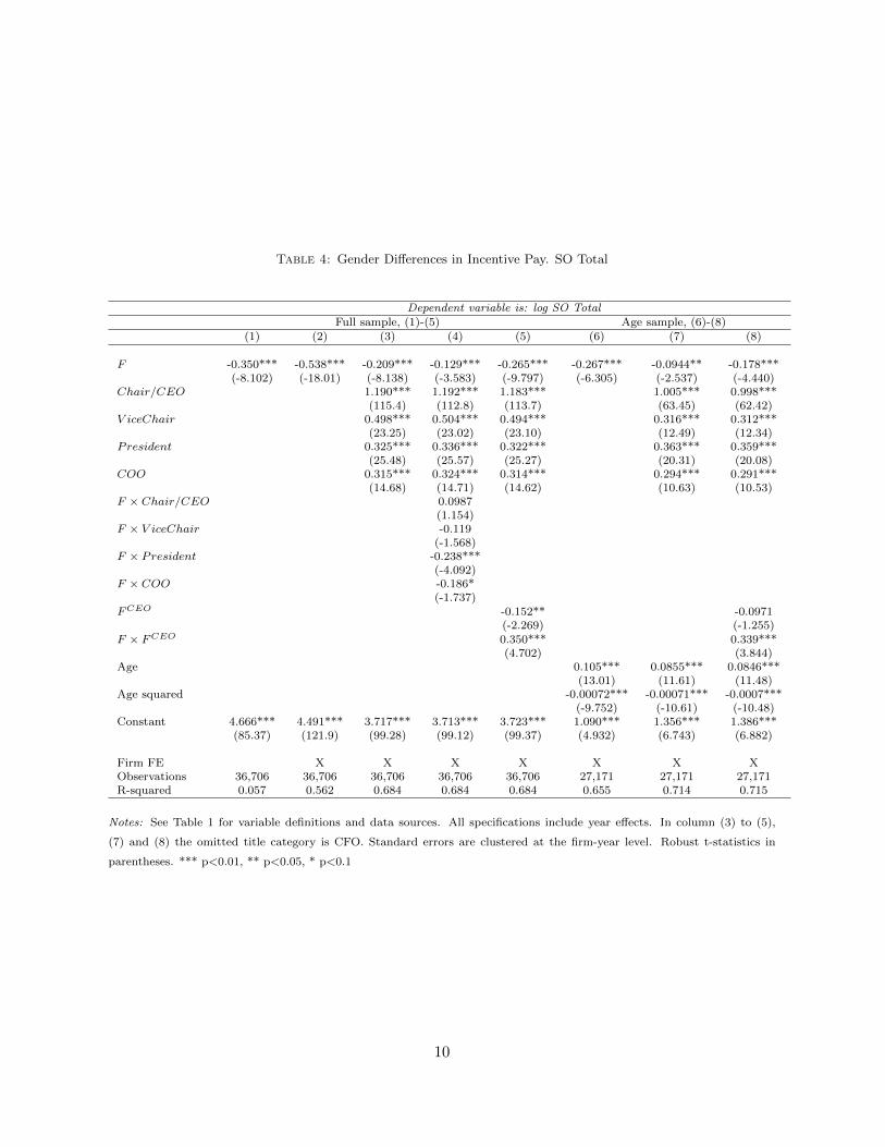
Table 4: Gender Differences in Incentive Pay. SO Total

Dependent variable is: log SO TotalFull sample, (1)-(5) Age sample, (6)-(8)

(1) (2) (3) (4) (5) (6) (7) (8)

F -0.350*** -0.538*** -0.209*** -0.129*** -0.265*** -0.267*** -0.0944** -0.178***(-8.102) (-18.01) (-8.138) (-3.583) (-9.797) (-6.305) (-2.537) (-4.440)

Chair/CEO 1.190*** 1.192*** 1.183*** 1.005*** 0.998***(115.4) (112.8) (113.7) (63.45) (62.42)

V iceChair 0.498*** 0.504*** 0.494*** 0.316*** 0.312***(23.25) (23.02) (23.10) (12.49) (12.34)

President 0.325*** 0.336*** 0.322*** 0.363*** 0.359***(25.48) (25.57) (25.27) (20.31) (20.08)

COO 0.315*** 0.324*** 0.314*** 0.294*** 0.291***(14.68) (14.71) (14.62) (10.63) (10.53)

F × Chair/CEO 0.0987(1.154)

F × V iceChair -0.119(-1.568)

F × President -0.238***(-4.092)

F × COO -0.186*(-1.737)

FCEO -0.152** -0.0971(-2.269) (-1.255)

F × FCEO 0.350*** 0.339***(4.702) (3.844)

Age 0.105*** 0.0855*** 0.0846***(13.01) (11.61) (11.48)

Age squared -0.00072*** -0.00071*** -0.0007***(-9.752) (-10.61) (-10.48)

Constant 4.666*** 4.491*** 3.717*** 3.713*** 3.723*** 1.090*** 1.356*** 1.386***(85.37) (121.9) (99.28) (99.12) (99.37) (4.932) (6.743) (6.882)

Firm FE X X X X X X XObservations 36,706 36,706 36,706 36,706 36,706 27,171 27,171 27,171R-squared 0.057 0.562 0.684 0.684 0.684 0.655 0.714 0.715

Notes: See Table 1 for variable definitions and data sources. All specifications include year effects. In column (3) to (5),

(7) and (8) the omitted title category is CFO. Standard errors are clustered at the firm-year level. Robust t-statistics in

parentheses. *** p<0.01, ** p<0.05, * p<0.1

10

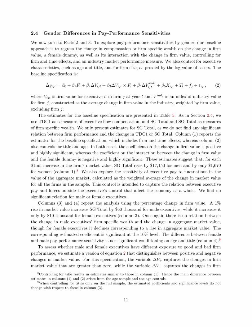
2.4 Gender Differences in Pay-Performance Sensitivities

We now turn to Facts 2 and 3. To explore pay-performance sensitivities by gender, our baseline

approach is to regress the change in compensation or firm specific wealth on the change in firm

value, a female dummy, as well as its interaction with the change in firm value, controlling for

firm and time effects, and an industry market performance measure. We also control for executive

characteristics, such as age and title, and for firm size, as proxied by the log value of assets. The

baseline specification is:

∆yijt = β0 + β1Fi + β2∆Vijt + β3∆Vijt × Fi + β4∆Vindjijt + β5Xijt + Tt + fj + εijt, (2)

where Vijt is firm value for executive i, in firm j at year t and V indj is an index of industry value

for firm j, constructed as the average change in firm value in the industry, weighted by firm value,

excluding firm j.

The estimates for the baseline specification are presented in Table 5. As in Section 2.4, we

use TDC1 as a measure of executive flow compensation, and SG Total and SO Total as measures

of firm specific wealth. We only present estimates for SG Total, as we do not find any significant

relation between firm performance and the change in TDC1 or SO Total. Column (1) reports the

estimates for the baseline specification, which includes firm and time effects, whereas column (2)

also controls for title and age. In both cases, the coefficient on the change in firm value is positive

and highly significant, whereas the coefficient on the interaction between the change in firm value

and the female dummy is negative and highly significant. These estimates suggest that, for each

$1mil increase in the firm’s market value, SG Total rises by $17,150 for men and by only $1,670

for women (column 1).8 We also explore the sensitivity of executive pay to fluctuations in the

value of the aggregate market, calculated as the weighted average of the change in market value

for all the firms in the sample. This control is intended to capture the relation between executive

pay and forces outside the executive’s control that affect the economy as a whole. We find no

significant relation for male or female executives.

Columns (3) and (4) repeat the analysis using the percentage change in firm value. A 1%

rise in market value increases SG Total by $60 thousand for male executives, while it increases it

only by $10 thousand for female executives (column 3). Once again there is no relation between

the change in male executives’ firm specific wealth and the change in aggregate market value,

though for female executives it declines corresponding to a rise in aggregate market value. The

corresponding estimated coefficient is significant at the 10% level. The difference between female

and male pay-performance sensitivity is not significant conditioning on age and title (column 4).9

To assess whether male and female executives have different exposure to good and bad firm

performance, we estimate a version of equation 2 that distinguishes between positive and negative

changes in market value. For this specification, the variable ∆V+ captures the changes in firm

market value that are greater than zero, while the variable ∆V− captures the changes in firm

8Controlling for title results in estimates similar to those in column (1). Hence the main difference betweenestimates in columns (1) and (2) arises from the age sample and the age controls.

9When controlling for titles only on the full sample, the estimated coefficients and significance levels do notchange with respect to those in column (3).

11

Table 5: Pay Performance Sensitivity. SG Total

Dependent variable is: ∆SGTotal(1) (2) (3) (4)

F 1,320 627.0 6,792 8,390(0.198) (0.0458) (1.189) (0.930)

∆V 17.15*** 20.08***(3.663) (3.588)

F ×∆V -15.48*** -16.58***(-3.314) (-2.819)

∆Vagg -0.212 -0.108 0.227 0.361(-0.235) (-0.0916) (0.272) (0.326)

F ×∆Vagg 0.318 0.228 -0.464 -0.591(1.014) (0.503) (-1.526) (-1.129)

%∆V 59,833*** 71,941***(3.015) (3.008)

F ×%∆V -49,828*** -87,133*(-2.460) (-1.678)

Title X XAge X XConstant 185,344** 375,152** 116,854 284,419

(2.288) (2.107) (1.122) (1.434)

Observations 28,257 22,266 28,257 22,266R2 0.104 0.124 0.020 0.026

Notes: See Table 1 for variable definitions and data sources. All specifications control for firm and year effects, logreal assets, and change in industry value. Standard errors are clustered at the firm-year level. Robust t-statisticsin parentheses. *** p<0.01, ** p<0.05, * p<0.1

12

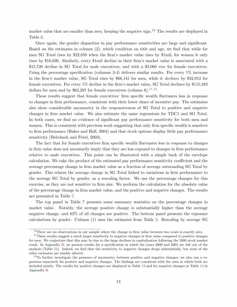
market value that are smaller than zero, keeping the negative sign.10 The results are displayed in

Table 6.

Once again, the gender disparities in pay performance sensitivities are large and significant.

Based on the estimates in column (2), which condition on title and age, we find that while for

men SG Total rises by $22,850 when the firm’s market value rises by $1mil, for women it only

rises by $16,030. Similarly, every $1mil decline in their firm’s market value is associated with a

$15,720 decline in SG Total for male executives, and with a $3,060 rise for female executives.

Using the percentage specification (columns 3-4) delivers similar results. For every 1% increase

in the firm’s market value, SG Total rises by $66,141 for men, while it declines by $32,912 for

female executives. For every 1% decline in the firm’s market value, SG Total declines by $115,482

dollars for men and by $62,297 for female executives (column 6).11,12

These results suggest that female executives’ firm specific wealth fluctuates less in response

to changes in firm performance, consistent with their lower share of incentive pay. The estimates

also show considerable asymmetry in the responsiveness of SG Total to positive and negative

changes in firm market value. We also estimate the same regressions for TDC1 and SO Total.

In both cases, we find no evidence of significant pay performance sensitivity for both men and

women. This is consistent with previous work suggesting that only firm specific wealth is sensitive

to firm performance (Baker and Hall, 2004) and that stock options display little pay performance

sensitivity (Bebchuck and Fried, 2003).

The fact that for female executives firm specific wealth fluctuates less in response to changes

in firm value does not necessarily imply that they are less exposed to changes in firm performance

relative to male executives. This point can be illustrated with a simple back of the envelope

calculation. We take the product of the estimated pay performance sensitivity coefficient and the

average percentage change in firm market value as a fraction of average outstanding SG Total by

gender. This relates the average change in SG Total linked to variations in firm performance to

the average SG Total by gender, as a rescaling factor. We use the percentage changes for this

exercise, as they are not sensitive to firm size. We perform the calculation for the absolute value

of the percentage change in firm market value, and the positive and negative changes. The results

are presented in Table 7.

The top panel in Table 7 presents some summary statistics on the percentage changes in

market value. Notably, the average positive change is substantially higher than the average

negative change, and 62% of all changes are positive. The bottom panel presents the exposure

calculations by gender. Column (1) uses the estimates from Table 5. Rescaling by average SG

10There are no observations in our sample where the change in firm value between two years is exactly zero.11These results suggest a much larger sensitivity to negative changes in firm value compared to positive changes

for men. We conjecture that this may be due to the large declines in capitalization following the 2000 stock marketcrash. In Appendix B, we present results for a specification in which the years 2000 and 2001 are left out of theanalysis (Table 12). Indeed, we find that the sensitivity to negative changes drops substantially, but none of theother estimates are sizably altered.

12To further investigate the presence of asymmetry between positive and negative changes, we also run a re-gression separately for positive and negative changes. The findings are consistent with the ones in which both areincluded jointly. The results for positive changes are displayed in Table 13 and for negative changes in Table 14 inAppendix B.

13

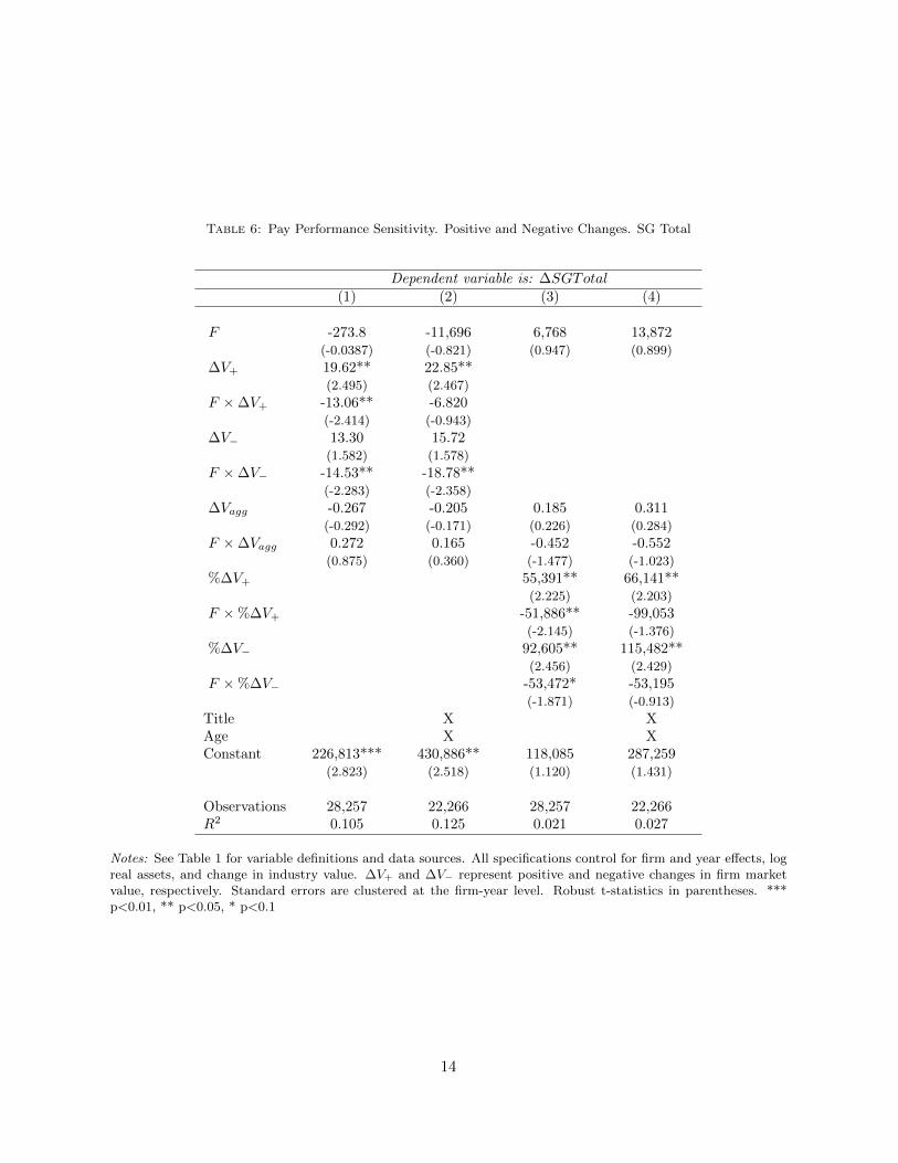
Table 6: Pay Performance Sensitivity. Positive and Negative Changes. SG Total

Dependent variable is: ∆SGTotal(1) (2) (3) (4)

F -273.8 -11,696 6,768 13,872(-0.0387) (-0.821) (0.947) (0.899)

∆V+ 19.62** 22.85**(2.495) (2.467)

F ×∆V+ -13.06** -6.820(-2.414) (-0.943)

∆V− 13.30 15.72(1.582) (1.578)

F ×∆V− -14.53** -18.78**(-2.283) (-2.358)

∆Vagg -0.267 -0.205 0.185 0.311(-0.292) (-0.171) (0.226) (0.284)

F ×∆Vagg 0.272 0.165 -0.452 -0.552(0.875) (0.360) (-1.477) (-1.023)

%∆V+ 55,391** 66,141**(2.225) (2.203)

F ×%∆V+ -51,886** -99,053(-2.145) (-1.376)

%∆V− 92,605** 115,482**(2.456) (2.429)

F ×%∆V− -53,472* -53,195(-1.871) (-0.913)

Title X XAge X XConstant 226,813*** 430,886** 118,085 287,259

(2.823) (2.518) (1.120) (1.431)

Observations 28,257 22,266 28,257 22,266R2 0.105 0.125 0.021 0.027

Notes: See Table 1 for variable definitions and data sources. All specifications control for firm and year effects, logreal assets, and change in industry value. ∆V+ and ∆V− represent positive and negative changes in firm marketvalue, respectively. Standard errors are clustered at the firm-year level. Robust t-statistics in parentheses. ***p<0.01, ** p<0.05, * p<0.1

14

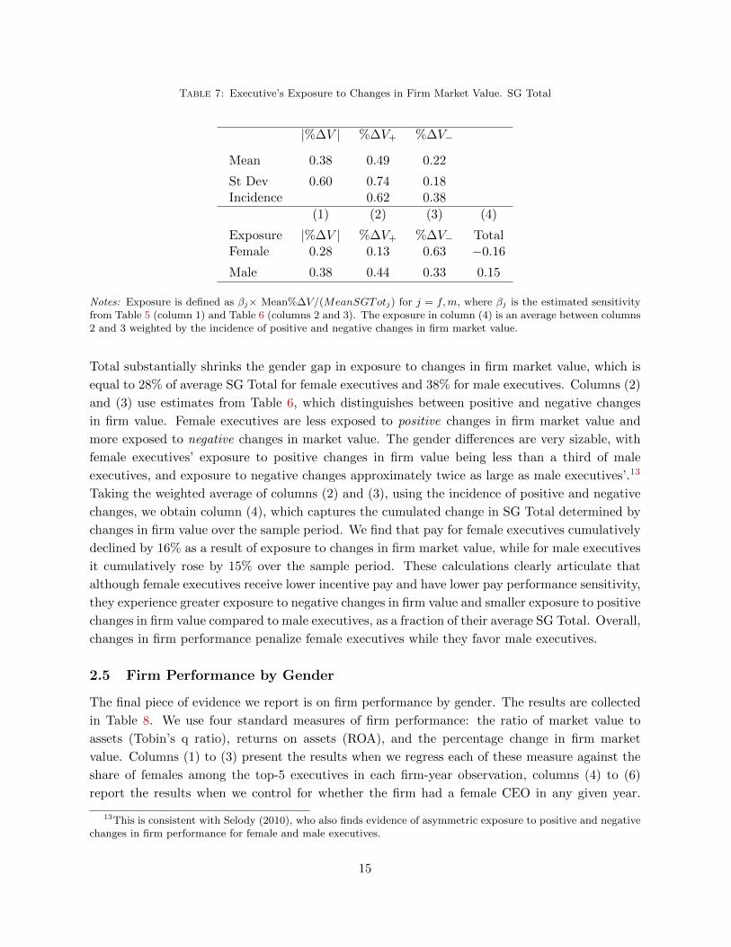
Table 7: Executive’s Exposure to Changes in Firm Market Value. SG Total

|%∆V | %∆V+ %∆V−

Mean 0.38 0.49 0.22

St Dev 0.60 0.74 0.18Incidence 0.62 0.38

(1) (2) (3) (4)

Exposure |%∆V | %∆V+ %∆V− TotalFemale 0.28 0.13 0.63 −0.16

Male 0.38 0.44 0.33 0.15

Notes: Exposure is defined as βj× Mean%∆V/(MeanSGTotj) for j = f,m, where βj is the estimated sensitivityfrom Table 5 (column 1) and Table 6 (columns 2 and 3). The exposure in column (4) is an average between columns2 and 3 weighted by the incidence of positive and negative changes in firm market value.

Total substantially shrinks the gender gap in exposure to changes in firm market value, which is

equal to 28% of average SG Total for female executives and 38% for male executives. Columns (2)

and (3) use estimates from Table 6, which distinguishes between positive and negative changes

in firm value. Female executives are less exposed to positive changes in firm market value and

more exposed to negative changes in market value. The gender differences are very sizable, with

female executives’ exposure to positive changes in firm value being less than a third of male

executives, and exposure to negative changes approximately twice as large as male executives’.13

Taking the weighted average of columns (2) and (3), using the incidence of positive and negative

changes, we obtain column (4), which captures the cumulated change in SG Total determined by

changes in firm value over the sample period. We find that pay for female executives cumulatively

declined by 16% as a result of exposure to changes in firm market value, while for male executives

it cumulatively rose by 15% over the sample period. These calculations clearly articulate that

although female executives receive lower incentive pay and have lower pay performance sensitivity,

they experience greater exposure to negative changes in firm value and smaller exposure to positive

changes in firm value compared to male executives, as a fraction of their average SG Total. Overall,

changes in firm performance penalize female executives while they favor male executives.

2.5 Firm Performance by Gender

The final piece of evidence we report is on firm performance by gender. The results are collected

in Table 8. We use four standard measures of firm performance: the ratio of market value to

assets (Tobin’s q ratio), returns on assets (ROA), and the percentage change in firm market

value. Columns (1) to (3) present the results when we regress each of these measure against the

share of females among the top-5 executives in each firm-year observation, columns (4) to (6)

report the results when we control for whether the firm had a female CEO in any given year.

13This is consistent with Selody (2010), who also finds evidence of asymmetric exposure to positive and negativechanges in firm performance for female and male executives.

15

Table 8: Firm Performance and Executives’ Gender

(1) (2) (3) (4) (5) (6)Performance Tobin Q ROA % ∆ MktVal Tobin Q ROA % ∆MktVal

%F -0.390* -0.154 -0.0936(-1.658) (-0.101) (-1.277)

FCEO -1.600 -3.028 0.0924*(-0.991) (-0.985) (1.648)

Constant 1.187*** 4.742*** 0.0826*** 1.181*** 4.836*** 0.0759***(7.674) (16.32) (6.302) (7.505) (16.28) (5.957)

Observations 14,012 14,078 12,634 13,710 13,772 12,400R-squared 0.481 0.358 0.186 0.482 0.378 0.192

Notes: See Table 1 for variable definitions and data sources. Robust t-statistics in parentheses. All specificationsinclude year effects and firm fixed effects. For each firm performance measure, we control for the correspondingindustry analog performance measure. Errors are clustered at the firm-year level. *** p<0.01, ** p<0.05, * p<0.1

All regressions control for time and year effects. We also control for the corresponding industry

performance measure in each specification.

The results suggest that there are no significant differences in firm performance by gender.

These findings are consistent with Catalyst (2004b) and Wolfers (2006). Wolfers analyzes 350

Fortune 500 companies in a broad range of industries and finds that the group of companies

with the highest representation of women in their top management team experienced better

performance than the group of companies ranked at the bottom in terms of female representation.

This holds for two measures of performance, Return on Equity and Return to Shareholders, in

the aggregate and by industry.14

3 Evidence of Gender Differences in Executive Labor Markets

We begin exploring the possible determinants of the gender differences in the structure of pay for

top executives by reviewing the evidence on gender differentials in characteristics that could be

relevant for the executive labor market. We examine three types of evidence: surveys of profes-

sionals and executives eliciting information on barriers to career advancement, time use evidence

on household allocation of child care responsibilities for top income earners, and experimental

and psychological studies of performance in competitive environments, propensity to compete

and initiate negotiations and risk aversion. Taken together, the evidence can be summarized as

follows:

• Exclusion from informal networks, gender stereotyping and lack of role models are perceived

as substantial barriers to career advancements for female executives.

14Bertrand and Schoar (2002) present evidence that “managerial style” influences not only performance but abroad range of corporate strategies such as capital structure, investment behavior, diversification policies and soon. Since managerial style can be interpreted as a collection of attributes and female and male executives differ inthese attributes (see Section 3), it is possible that firm strategy varies based on the gender of the top executives,even if this is not reflected in systematic differences in performance.

16

• Married women in the top 5% of the income distribution bear a disproportionately large

share of child care responsibilities relative to married men in similar circumstances.

• Women display lower performance in competitive environments, even with no differences

in performance in non-competitive setting, and lower propensity to select into competitive

environments.

• Women display lower propensity to initiate negotiations.

• Women exhibit higher risk tolerance to abstract gambles, but there are no gender differences

in risk aversion in contextual financial settings.

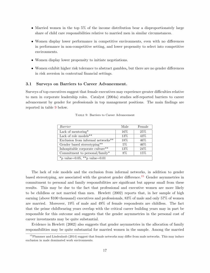
3.1 Surveys on Barriers to Career Advancement.

Surveys of top executives suggest that female executives may experience greater difficulties relative

to men in corporate leadership roles. Catalyst (2004a) studies self-reported barriers to career

advancement by gender for professionals in top management positions. The main findings are

reported in table 9 below.

Table 9: Barriers to Career Advancement

Barrier Male Female

Lack of mentoring* 16% 25%Lack of role models** 13% 43%Exclusion from informal networks** 18% 46%Gender based stereotyping** 5% 46%Inhospitable corporate culture** 13% 24%Commitment to personal/family* 8% 15%

*p value=0.05, **p value=0.01

The lack of role models and the exclusion from informal networks, in addition to gender

based stereotyping, are associated with the greatest gender difference.15 Gender asymmetries in

commitment to personal and family responsibilities are significant but appear small from these

results. This may be due to the fact that professional and executive women are more likely

to be childless or not married than men. Hewlett (2002) reports that, in her sample of high

earning (above $100 thousand) executives and professionals, 83% of male and only 57% of women

are married. Moreover, 19% of male and 49% of female respondents are childless. The fact

that the prime childbearing years overlap with the critical career building years may in part be

responsible for this outcome and suggests that the gender asymmetries in the personal cost of

career investments may be quite substantial.

Evidence in Hewlett (2002) also suggests that gender asymmetries in the allocation of family

responsibilities may be quite substantial for married women in the sample. Among the married

15Plummer and Lindenlaub (2014) suggest that female networks may differ from male networks. This may induceexclusion in male dominated work environments.

17

professionals and top executives, only 39% of men are married to women who are employed full

time, and 40% of these spouses earn less than $35 thousand a year. On the other hand, 90% of

women in the high achieving category have husbands who are employed full time or self-employed,

and 25% are married to men who earn more than $100 thousand a year. Among her sample of

high achieving women with husbands working full time, 51% take time off for child sickness, while

only 9% of men do. Similarly, 61% of women are mainly responsible for organizing child activities,

while only 3% of men bear this responsibility.

These results lead us to consider more systematic evidence on the allocation of child care and

family responsibilities for high earning individuals using time use data.

3.2 Time Use for Top Income Earners

Table 15 reports information on weekly hours spent in child care activities, as well as total home16

and market hours for workers in the top 5% of the income distribution in the American Time Use

Survey (ATUS). The sample has been selected to reflect the characteristics of individuals in the

ExecuComp data set as closely as possible while maximizing the number of observations. The

sample includes 171 women and 496 men. We also report information for the overall population

to facilitate comparisons.

Two main facts emerge from the analysis of the table:

• Gender differences in total weekly hours spent in home production activities are smaller for

top earners than in the overall population. For the sample of married men and women the

ratio of female to male home hours is 1.38 (column 5) and 1.73 in the overall population

(column 1).

• Gender differences in time spent in the care of children do not vary much by income. The

ratio of female to male hours of child care full for married individuals is 2.4 for top 5%

income earners and 2.3 in the overall population. For the top 5% of earners, married women

with children under 5 spend 25.2 hours per week on child care, while married men only

spend 10.2 hours (column 9).

This analysis cannot be directly brought to bear on the sample of top executives in ExecuComp

due to top coding of incomes in ATUS. Yet, the substantial gender asymmetry in child care

responsibility may ultimately affect women’s career advancement and exert a permanent effect on

their behavior in market work.

3.3 Evidence on Gender Differences in Preferences

There is a large and active experimental literature exploring gender differences in preferences.

The literature is extensively and critically reviewed in Bertrand (2010), Niederle (forthcoming)

and Azmat and Petrongolo (forthcoming). Here, we summarize the main findings to frame the

discussion is Section 4.

16Home production measures exclude any child care related hours in ATUS.

18

Performance in Competition and Propensity to Compete Experimental evidence sug-

gests that women may be less effective than men in competitive environments, even if they demon-

strate the same ability to perform in noncompetitive environments (Gneezy, Niederle and Rusti-

chini, 2003). In addition, women have lower propensity to select into competitive environments

(Niederle and Vesterlund, 2007) and seek challenges (Niederle and Yenstruskas, 2007).

Propensities to Initiate Negotiations Babcock and Laschever (2003) present a variety of

evidence, in the form of surveys, case studies and interviews, suggesting that women exhibit

lower propensity to initiate negotiations. These findings are refined in a variety of experimental

settings.17 Consistently, women asked for greater compensation much less often than men. Social

incentives and situational factors appear to play a critical role, based on the differential treatment

of men and women when they attempt to negotiate.

Risk Aversion Survey evidence and field studies based on asset allocations suggest that women

have higher risk aversion than men.18 However, survey respondents are prone to evaluate the risks

they are confronted with based on their individual opportunity sets, and controls for individual

wealth and earnings are either weak or absent from the analysis. There is also a sizable experi-

mental literature with findings broadly consistent with higher risk aversion for women (see Croson

and Gneezy, 2009, and Eckel and Grossman, 2008). Even if this evidence is rather inconclusive

(Niederle, forthcoming), some systematic patterns increases confidence in these results. For exam-

ple, lack of confidence can result in reduced tolerance towards risk (Bertrand, 2010) and women’s

lower propensity to initiate negotiation is also consistent with male overconfidence. Moreover,

the findings in economics are consistent with psychological evidence on gender differences in risk

taking.19

The available evidence is broadly consistent with a systematic difference in preferences across

genders. Yet, high level managers undergo a severe process of (self-)selection, thus one would

expect them to exhibit a comparative advantage in essential traits, such as ability to form and

join networks, perform in competitive environments, propensity to negotiate and to embrace

risk.20 Even if gender differences in preferences are small for this group, combined with additional

systematic differences, such as the costs of career investments or weight of family responsibilities,

they may influence an executive’s ability to influence firm performance or effect the value to the

17See Riley and Babcock (2002), Small, Gellman, Babcock and Gettman (2005) and Bowles, Babcock, and Lai(2005).

18Barsky, Juster, Kimball, and Shapiro (1997) find that females display smaller risk tolerance than males basedon survey responses in the Health and Retirement Study. Portfolio evidence also suggests that wealth holdings ofsingle women are less risky than those of single men of equal economic status (Jianakoplos and Bernasek, 2009, andSunden and Surette, 1998).

19The strongest support for gender differences in risk attitudes in the psychological literature comes from patternsof risky sex and risky driving behavior. See Byrnes, Miller, and Schafer (1999).

20In a natural field experiment with college students, Samek (2015) ratifies the finding that women are deterredby performance based compensation schemes more than men, controlling for risk preferences. However, when con-trolling by major, she finds that students of Business and Engineering of both genders strongly prefer a competitivescheme.

19

executive of a given compensation package.

To explore the effects of these factors on executive compensation, we view the pay setting

process as an agency problem. In Section 4, we explore the efficient contracting paradigm of

executive compensation and the skimming or executive power view to assess whether they can

rationalize some of the gender differences in executive pay.

4 Executive Compensation Paradigms: Efficient Contracting vs

Managerial Power

In this section, we compare two paradigms for executive compensation. The first is the efficient

benchmark, based on a dynamic moral hazard model in which shareholders set pay for top firm

executives to optimally trade-off insurance and incentive provision. The second is based on recent

evidence that managerial compensation is not efficient, and is instead driven by the entrenched

managers who hold board captives and are able to set the terms of their own pay. We will

then assess − based on the differences in preferences and entrenchment between female and male

executives − which paradigm can rationalize the gender differences in compensation structure for

top executives described in Section 2.

4.1 Efficient Contracting Benchmark

We start from the benchmark efficient paradigm for executive compensation which is based on

the arm’s length model of interaction between shareholders and executives. The shareholders

(principals) hire an executive (agent) to manage the firm. They set executive compensation to

maximize the surplus from the executive-firm relationship. Time, t, is discrete. The executive’s

effort, et, influences the growth in firm value, Vt, according to the law of motion:

Vt+1 − Vt = b (Vt) et + ω (Vt) . (3)

The term b (Vt) et corresponds to the expected change in firm value, and the parameter b (V )

represents the impact of the executive’s effort, or the marginal product of managerial effort. The

term ω (Vt) is a random variable distributed normally with zero mean and standard deviation

Σ (Vt) > 0. Following Baker and Hall (2004), both the expected change in firm value and its

volatility are allowed to depend on firm value, which is a proxy for size.

The executive’s preferences are represented by the utility function:

U (w, e) = − exp (−σ [w − θv (e)]) , (4)

where w corresponds to earnings. The coefficient of absolute risk aversion is σ > 0, and v (·)denotes the disutility of effort, where e ∈ [0, 1]. The function v is increasing, twice continuously

differentiable and convex. The parameter θ > 0 represents the cost of effort for the executive. We

adopt a CARA utility specification to allow for a closed form solution.

A moral hazard problem arises since effort, e, is private information. Effort should be in-

20

terpreted broadly, as any action that increase firm value but generates a non-pecuniary cost for

the executive. In a literal interpretation, low values of effort would correspond to shirking. Al-

ternatively, lower values of effort 1 can be interpreted as an action that reduces firm value but

generates private benefits for the executive, such as perks.

The change in firm value, Vt−Vt−1, is observable. The optimal compensation contract specifies

an effort level and an earnings function, linking earnings, w, to the change in firm value ∆Vt =

Vt − Vt−1. Since the change in firm value is the only observable measure of the executive’s

performance, a dependence of earnings on this variable is essential for the contract to implement

strictly positive effort, given the agency problem.

The expected surplus from the firm-executive relationship is equal to its certainly equivalent:

ES (e) = b (V ) e− θv (e)− σ (Σ (V ))2 (w)2 /2. (5)

The first term is expected change in firm value, the second term is the utility cost of exerting

effort for the executive. The last term corresponds to the reduction in the executives’ utility due

to the fact that her earnings depend on firm performance and are thus stochastic. If the executive

is risk averse, that is σ > 0, the resulting earnings volatility reduces her utility.

The optimal compensation contract maximizes the expected surplus from the shareholder-

executive relationship subject to an incentive compatibility and a participation constraint for the

executive, which reflects the executive’s outside option. The optimal contract specifies the execu-

tive’s earnings as a function of the observable change in firm value. As shown in Holmstrom and

Milgrom (1991), CARA utility implies that, without loss of generality, we can restrict attention

to earnings functions of the form: w (∆V ) = w + w∆V, where w corresponds to cash salary and

w∆V is incentive pay. The incentive pay component, w∆V, can be taken to correspond the sum

of of all components of compensation that are sensitive to firm performance, such as bonus pro-

grams and restricted stock and stock options grants. The linear structure of the model delivers

the following predictions for the growth in executive earnings:

∆wt = ∆wt + w (∆Vt −∆Vt−1) .

where ∆wt = wt − wt−1. Thus, w corresponds to pay-performance sensitivity.21

We describe all the remaining analytical details pertaining to the derivation of the optimal

compensation contract in Appendix C. Proposition 1 describes the properties of the optimal

compensation contract as a function of the executive’s attributes, which, together with some

firm characteristics, determine whether effort is maximized or interior. The proposition is stated

formally in the appendix. Here, we simply restate the properties of the optimal contract salient

to our analysis, in comparative statics terms.

21This has a direct counterpart in the conventional pay-performance sensitivity regression:

∆wt = α0 + α1∆Vt + εt.

This specification implies that α0 = ∆wt − w∆Vt−1 and α1 = w under the null that the model is true.

21

Properties of the optimal compensation contract Proposition 1 delivers the following

comparative statics results on the link between optimal compensation and the executive’s at-

tributes for given firm size for interior effort:

• Optimal effort is maximized if and only if:

θ

b(V )

(1 +

σ

b(V )

Σ2

b(V )

)≤ 1. (6)

• If optimal effort is interior:

– Effort is increasing in b and declining in θ, σ and Σ.

– Pay-performance sensitivity, w, is increasing in b and declining in θ, σ and Σ.

– Cash salary, w, and total compensation, w, are increasing in b and decreasing in θ, σ

and Σ, as well as increasing in u.

• If optimal effort is maximized:

– Pay-performance sensitivity, w, is increasing in θ and declining in b. It does not vary

with σ and Σ.

– Cash salary, w, and total compensation, w, are decreasing in b and increasing in θ, σ

and Σ, as well as increasing in u.

The value of b (V ) is critical for the optimal value of effort. Given the executive’s cost of effort

and risk aversion, θ and σ, and the performance volatility, Σ2, effort will be maximized when the

impact of the executive’s effort on the change in firm value is sufficiently large.

The cost of providing incentives is increasing in θ and σ and declining in b. Moreover, higher

volatility of the change in firm value, Σ, reduces the ability of the observed change in value to serve

as a signal for the executive’s effort, making the moral hazard problem more severe. Therefore,

optimal effort is maximized when the effectiveness of the executive, b, is high enough relative to

the cost of providing incentives.

The optimal structure of compensation depends on whether effort is maximized. When effort

is interior, the impact of the executive on firm performance via effort is relatively low. Since it is

costly to incentivize the executive, the optimal effort will be declining in θ, σ and Σ, and so will

be the fraction of incentive pay, salary and total compensation. Since salary, w, does not influence

the executive’s effort, it does not enter the surplus and only influences its division between the

firm and the executive. The salary is increasing in b, decreasing in θ, σ, and Σ, and increasing in

u. The same comparative statics relationships holds for overall compensation, w.

If effort is maximized, then the executive has high impact and the optimal contract com-

pensates the executive for exerting the maximum effort in an incentive compatible fashion by

making incentive pay and total compensation decreasing in b and increasing in the executive’s

cost of effort θ. It does not depend on the executive’s risk aversion or Σ. A higher value of b

generates an intrinsically high sensitivity of firm performance to the executive’s effort, and thus

22

reduces the level of w required to implement the maximum effort. By contrast, a higher cost of

effort requires higher sensitivity of pay to firm performance to induce the executive to exert the

maximum effort level. Salary and total compensation are also increasing in θ and declining in b,

as well as increasing with both σ and Σ.

By equation (15), effort is maximized for b (V ) /θ large enough. Thus, the elasticity of b (V )

with respect to firm value V is a critical parameter. Moreover, in this framework, firm value also

corresponds to firm size. To fully characterize the structure of the optimal contract, specifically,

the dependence of salary and incentive pay on the executive’s attributes, we embed the efficient

contracting model into an equilibrium assignment model. Following Baker and Hall (2004), we

assume:

b (V ) = bV γ , (7)

ω (V ) = ωV γ , (8)

where b, ω > 0 and γ ∈ [0, 1] corresponds to the elasticity of the impact of effort on firm perfor-

mance. This flexible formulation allows us to capture most cases considered in the literature. If

this elasticity is zero, then the marginal product of executive effort is invariant to firm size. At

the other extreme, if the marginal product of effort varies one to one with firm size, the impact

of effort will rise with firm size. This assumption underlies the classic span of control models of

Lucas (1978) and Rosen (1982). The power of incentives corresponds to the change in expected

pay perceived by the executive as effort changes, and with this formulation it corresponds to

wbV γ , which depends on whether effort is maximized and on firm value.

The optimal firm size distribution of executives maximizes economy wide surplus, as described

in detail in Appendix C, by assigning value to executives with different attributes. The solution

to the assignment problem is described in Proposition 2. The main results in that proposition are

that if optimal effort is interior, all executives will be assigned strictly positive firm value. The

optimal value is increasing in b for γ < 1. By contrast, when effort is maximized, executives with

undesirable characteristics will not be assigned a strictly positive firm value. The highest ranked

executive will be assigned all the value outstanding capital.

The properties of the optimal assignment problem suggests that the case in which the optimal

level of effort is 1 is non generic, as it corresponds to a situation in which the most desirable

executive manages all capital. For this reason, we restrict attention to the predictions of the

model with interior optimal effort for the rest of our discussion.

Hypothesis Regarding Gender Differences The empirical evidence discussed in Section 3

suggests that executive women are less able to be included in professional networks and find men-

tors, and they experience higher costs of career investments and bear a larger share of child care

responsibilities. Moreover, women show lower propensity to compete and initiate negotiations,

and they display lower risk tolerance.

The executive labor market is highly competitive, entails constant negotiations, involves bear-

ing risk and is mostly male. Networking and mentoring are seen as key to professional advance-

23

ment. In addition, a high number of work hours is required, making it hard to reconcile these

positions with responsibilities outside of work. Thus, if the gender differences described in Section

2 are present among top executives, they may exert a significant influence on women’s perfor-

mance on the executive labor market. We now discuss a possible mapping between these gender

differences discussed in Section 3 and the vector of executive attributes in the agency model

n = b, σ, θ, u .Female executives’ lack of access to professional networks and mentors could both reduce their

impact on firm value b, and increase their cost of managerial effort θ. Women’s higher cost of

career investment and greater burden of family responsibility could be taken to correspond to

higher value of θ for female executives relative to males.

Women’s lower propensity to compete or engage in negotiations may be represented as entailing

a higher utility cost of exerting managerial effort, that is a higher value of θ for female executives.

These traits could also reduce the impact of effort on firm performance, that is the parameter b.

Higher θ or lower b would both lead to lower incentive pay as a share of total compensation and

lower pay-performance sensitivity, for given firm size.

The evidence on women’s lower risk tolerance implies a higher coefficient of relative risk

aversion for female executives. As discussed in Baker and Hall (2004), there is an inverse relation

between absolute risk aversion and the executive’s wealth, for given coefficient of relative risk

aversion, σR:

σ = σR/W,

where W is the executive’s wealth. The female executives’ lower earnings would imply a lower

value of wealth, which would determine a higher value of their coefficient of absolute risk aversion.

The executive’s outside option u only influences the level of cash salary and total earnings.

There is no direct connection between the evidence in gender differences may influence u. If

the outside option corresponds to the next best executive position, women’s reported greater

difficulties in accessing professional networks, may entail lower values of u for women.

To summarize, the empirical findings on the gender differences in structure of compensation

are consistent with female executives having low b, high θ and σ relative to men. Should we then

conclude that the gender differences in pay in the executive labor markets are efficient? Such a

conclusion would be unwarranted, given that the efficient contracting model cannot account for

many of the empirical findings we discuss in Section 2. First, after conditioning on all observables,

we do not find any significant differences in firm performance in relation to the female presence

in executive positions. The efficient model predicts that lower effort will be implemented for

executives with lower b or higher σ and θ, leading to lower average performance, as measured by

the change in firm value. This contradicts the evidence. The efficient model predicts that women

should receive lower fraction of incentive and exhibit lower pay-performance sensitivity, as we find

in the data. However, the model cannot explain why female top executives are less exposed to

good firm performance and more exposed to bad in firm performance relative to males.

We now turn to an alternative model of executive compensation to examine these issues.

24

4.2 Alternative Views of the Pay-Setting Process

The efficient contracting approach to executive compensation assumes that compensation packages

are generated by arms length contracting between executives and a principal, possibly representing

the board of directors, who seek to maximize the value of the firm for shareholders. However,

Bebchuk and Fried (2003 and 2005) criticize this approach and propose instead that executive

compensation depends on managerial power. The heart of their hypothesis is that board members

also face an agency problem, which implies that they cannot be taken to make decisions to

maximize the shareholders’ value. Then, executives can influence their compensation package to

increase average pay and undermine incentives. Bertrand and Mullainathan (2001) refer to this

paradigm as skimming and suggest that in this case CEOs can act like ”agents without principals.”

Such behavior may give rise not only to higher average executive pay but also to distortions to

incentives, such as rewarding for growth in size, low sensitivity to firm performance, excessive risk

taking and so on.

Bebchuk and Fried (2003) summarize the factors that may make board members sensitive

to executive power when setting compensation packages. These include the incentive to be re-

elected, the CEO’s ability to reciprocate directors for favors, participation in informal networks

leading to loyalty and incentives for reciprocity towards the executive by the board, cognitive

dissonance stemming from executive positions currently or previously held by board members,

and ratcheting resulting from competition on executive labor markets. They argue that market

forces do not have the ability to restrain these enabling factors.

According to this view, the only social stigma faced by executives who receive disproportion-

ately large compensation may limit the degree to which CEOs can exert influence over their own

pay. This leads to efforts on part of executives to camouflage their earnings, by using stock options

and other less visible forms of compensation, such as executive pension plans, deferred compen-

sation and post-retirement perks (Kuhnen and Zwiebel, 2009). The social costs of increasing top

executive compensation may vary with aggregate stock market performance and decline in good

times. Thus, executive compensation may rise more steeply in periods of good firm and stock

market performance. The level and structure of executive pay will also be sensitive to corporate

governance variables.

Pay-Perfomance Links The managerial power or skimming view predicts that the links be-

tween executive pay and firm performance will be weak. It argues that components of compen-

sation that are officially presented as incentive pay, may easily be structured so that they do

not expose the executive to bad firm performance. In particular, equity based compensation

can be designed so that executives executive can gain from any increase in the nominal value of

the stock price above the grant-date market value. This implies that executives can experience

gains in pay even if their firm performs below the relevant peer group, as long as market-wide

and industry-wide movements provide sufficient lift for the stock price. Thus, compensation will

be more sensitive to increases in firm value than declines, and should increase with aggregate

market value and other factors that positively affect firm performance but are completely outside

the scope of influence top executives. Results in Bertrand and Mullainathan (2001) suggest that

25

CEOs are indeed rewarded for these factors.

Kuhnen and Zwiebel (2009) provide a formalization of this view and derive the implications

for the relation between executive attributes and the structure of pay. Their analysis focusses on

the hidden components of pay. They posit that direct salary and bonuses are the most observ-

able components of compensation, while other forms of pay are hidden. The main predictions of

their theoretical analysis are that hidden pay is increasing in the noise in the production process

(corresponding to Σ in the notation introduced in Section 4.1), the manager’s outside option

(corresponding to u) and decreasing in the uncertainty over the manager’s ability or talent (cor-

responding to b), which they proxy with the inverse of a manager’s tenure in their empirical

analysis. Their results are strongly supportive of the model’s prediction for a sample of CEOs.

We now use the findings in Section 2 to assess the skimming view of executive pay.

Gender and Managerial Power The fact that female top executives perceive limited access

to informal networks, gender stereotyping, an inhospitable corporate culture, jointly with their

younger age and lower tenure, suggests that they might be considerably less entrenched and exert

lower control on their own compensation than their male counterparts on average. It follows that,

if the skimming view is correct, female compensation packages should display fewer of the features

that are predicted by the managerial power model.

The evidence on the structure of pay and pay-perfomance sensitivity is consistent with this

hypothesis. We find that female executives have much lower incentive/hidden pay in the form

of stock options, stock grants and firm specific wealth. Moreover, while female top executives

experience lower pay performance sensitivity than male top executives, female executives reap a

lower gain in case of positive firm performance relative to male executives, and experience larger

declines in firm specific wealth in case of declines in firm performance.

5 Concluding Remarks

The efficient contracting model can rationalize several of the gender differences in the structure of

compensation for top executives, based on the experimental and survey evidence on gender differ-

ences in preferences and costs of managerial effort. However, the efficient compensation contract,

reflecting these perceived differences in attributes, would induce lower effort for female managers,

resulting in lower effective performance relative to males. We find no differences in measured firm

performance based on the percentage of women in top executive positions. The efficient contract-

ing paradigm also fails to explain why female executives’ earnings are more exposed to bad firm

performance. The managerial power/skimming view of executive compensation can rationalize

these differences based on the notion that female top executives are less entrenched than male top

executives, due to their younger age and their relative difficulties in accessing informal networks.

These two views of the pay-setting process lead to a very different assessment both of the

level and structure of pay for top executives. Under the efficient contracting paradigm, the

gender differences in pay are optimal based on the gender differences in attributes. The lack of

representation of women in top executive positions is inconsequential. Based on the skimming

26

view, the gender differences in pay do no reflect any performance relevant characteristic, but

different degrees of managerial power of female and male executives. Based on this explanation, it

would be optimal to have more women in top executive positions, even if they have less desirable

attributes as managers, as long as they remain less entrenched than men. More broadly, the

fact that the skimming view is able to rationalize more of the gender differences in the level

and structure of pay raises additional questions about the validity of the efficient contracting

paradigm.

27

References

[1] Mark Aguiar and Erik Hurst, 2007. Measuring Trends In Leisure: The Allocation Of Time

Over Five Decades. Quarterly Journal of Economics 122 (3): 969-1006.

[2] Stefania Albanesi and Claudia Olivetti, 2009. Home production, market production and the

gender wage gap: Incentives and expectations. Review of Economic Dynamics 12 (1): 80-107.

[3] Ghazala Azmat and Barbara Petrongolo, 2015. Gender and the labor market: What have we

learned from field and lab experiments? Forthcoming, Labour Economics.

[4] Linda Babcock and Sara Laschever, 2003. Women Don’t Ask: Negotiation and the Gender

Divide Princeton University Press.

[5] George Baker and Brian Hall, 2004. CEO Incentives and Firm Size. Journal of Labor Eco-

nomics 22(4): 767-798.

[6] Lucian A. Bebchuk and Jesse M. Fried, 2003. Executive Compensation as an Agency Problem.

The Journal of Economic Perspectives 17(3): 71-92.

[7] Lucian A. Bebchuk and Jesse M. Fried, 2005. Pay Without Performance: Overview of the

Issues. Journal of Applied Corporate Finance 17(4): 8-23.

[8] Linda A. Bell, 2005. Women-Led Firms and the Gender Gap in Top Executive Jobs. IZA DP

No. 1689

[9] Marianne Bertrand, 2011. New Perspectives on Gender. Handbook of Labor Economics 4:

1543-1590.

[10] Marianne Bertrand and Kevin Hallock, 2001. The Gender Gap in Top Corporate Jobs. In-

dustrial and Labor Relations Review, Vol. 55, No.1.

[11] Marianne Bertrand and Sendhil Mullainathan, 2001. Are CEOs Rewarded for Luck? The

Ones Without Principlas Are. Quarterly Journal of Economics 116(3): 901-932.

[12] Marianne Bertrand and Antoinette Schoar, 2003. Managing With Style: The Effect of Man-

agers on Firm Policies. Quarterly Journal of Economics 118(4): 1169–1208.

[13] James Byrnes, David Miller and William Schafer. 1999. Gender Differences in Risk Taking:

A Meta-Analysis. Psychological Bulletin 125(3): 367-383.

[14] Catalyst, 2004a. Women and Men in U.S. Corporate Leadership.

[15] Catalyst, 2004b. The Bottom Line: Connecting Corporate Performance and Gender Diver-

sity.

[16] Rachel Croson, and Uri Gneezy. Gender differences in preferences. Journal of Economic

literature (2009): 448-474.

28

[17] Catherine C. Eckel and Philip J. Grossman. Differences in the economic decisions of men

and women: Experimental evidence. Handbook of experimental economics results 1 (2008):

509-519.

[18] Alexander Edmans, Xavier Gabaix, and Augustin Landier. 2007. A Calibrated Model of

Optimal CEO Incentives in Market Equilibrium. NBER WP 13372.

[19] Xavier Gabaix and Augustin Landier, 2007. Why has CEO pay Increased so much? Quarterly

Journal of Economics.

[20] George-Levy Gayle, Limor Golan and Robert A. Miller, 2012. Gender Differences in Executive

Compensation and Job Mobility. Journal of Labor Economics, Vo. 30(4): 829-71.

[21] Uri Gneezy, Muriel Niederle, and Aldo Rustichini, 2003. Performance in Competitive Envi-

ronments: Gender Differences. Quarterly Journal of Economics CXVIII: 1049 – 1074.

[22] Brian J. Hall; Kevin J. Murphy, 2003. The Trouble with Stock Options. The Journal of

Economic Perspectives. 17(3): 49-70.

[23] Sylvia A. Hewlett, 2002. Executive Women and the Myth of Having It All. Harvard Business

Review.

[24] Charles P. Himmelberg and R. Glenn Hubbard, 2000. Incentive Pay and the Market for CEOs:

An Analysis of Pay-for-Performance Sensitivities, Presented at Tuck-JFE Contemporary Cor-

porate Governance Conference. Available at SSRN: http://ssrn.com/abstract=236089.

[25] Bengt Holmstrom, 1979. Moral Hazard and Observability. Bell Journal of Economics X:

74-91.

[26] Michael C. Jensen and Kevin J. Murphy, 1990. Performance Pay and Top-Management In-

centives, Journal of Political Economy, Vol. 98, 225-264.

[27] Nancy Jianakoplos and Alexandra Bernasek, 1998. Are Women More Risk Averse? Economic

Inquiry 36: 620-630.

[28] Camelia Kuhnen and Jeffrey Zwiebel. 2009. Executive Pay, Hidden Compensation and Man-

agerial Entrenchment. Manuscript, UNC.

[29] Peggy Lee and Erika James, 2003. She-E-Os: Gender Effects and Stock Price Reactions to

the Announcements of Top Executive Appointments. Darden Business School Working Paper

02-11.

[30] Thomas Lemieux, W. Bentley MacLeod and Daniel Parent, 2009. Performance Pay and Wage

Inequality. The Quarterly Journal of Economics 124(1): 1-49.

[31] Robert E. Lucas, 1978. On The Size Distribution of Business Firms. The Bell Journal of

Economics 9(2): 508-523.

29

[32] Nancy Mohan and Carl Chen, 2004. Are IPOs Priced Differently Based on Gender? Journal

of Behavioral Finance 5(1): 57-65.

[33] Kevin J. Murphy, 1986. Incentives, Learning, and Compensation: A Theoretical and Empir-

ical Investigation of Managerial Labor Contracts, The Rand Journal of Economics, Vol. 17,

59-76.

[34] Muriel Niederle. Gender. Handbook of Experimental Economics, second edition. Eds. John

Kagel and Alvin E. Roth, forthcoming.

[35] Muriel Niederle and Lise Vesterlund, 2007. Do Women Shy Away from Competition? Do

Men Compete too Much?, Quarterly Journal of Economics, forthcoming, August.

[36] Ilse Prummer and Anja Lindenlaub, 2014. Gender, Social Networks, and Performance.

Cambridge-INET Institute Working Paper No.12.

[37] Sherwin Rosen, 1982. Authority, Control, and the Distribution of Earnings. The Bell Journal

of Economics 13(2): 311-323.

[38] Anya Samek, 2015. A University-Wide Field Experiment on Gender Differences in Job Entry

Decisions. Manuscript, UWM.

[39] Michael Sattinger, 1993. Assignment Models of the Distribution of Earnings. Journal of

Economic Literature 31(2): 831-880.

[40] Karen Selody, 2010. Is the risk worth the reward for female executives? Manuscript, Depart-

ment of Economics, University of California, Berkeley.

[41] Deborah Small, Michele Joy Gelfand, Linda C. Babcock and Hilary Gettman, 2005. Who Gets

to the Bargaining Table? Understanding Gender Variation in the Initiation of Negotiations.

IACM 17th Annual Conference Paper.

[42] Annika Sunden and Briasn Surette, 1998. Gender differences in the allocation of assets in

retirement savings plans. American Economic Review 88(2): 207-11.

[43] Marko Tervio, 2007. The Difference that CEOs Make: An Assignment Model Approach.

Manuscript, University of California, Berkeley.

[44] Cheng Wang, 1997. Incentives, CEO Compensation, and Shareholder Wealth in a Dynamic

Agency Model, Journal of Economic Theory, Vol. 76, 72-105.

[45] Justin Wolfers, 2006. Diagnosing Discrimination: Stock Returns and CEO Gender. Journal

of the European Economic Association 4(2-3): 531-541.

30

A Data Appendix

A.1 Sample selection

Our sample is built according to the following criteria:

• Execucomp sample 1992-2005. This is because 2006 disclosure reform which makes data on

TDC1, Stock Options and Stock Grants not fully comparable to pre-2006 data.

• Excludes firms who are not in the S&P500, S&P MidCap 400 and S&P Small Cap 600.

• We drop duplicate observations based on the following variables: ”gvkey year co per r tcc

tdc1 tdc2 salary bonus shrown t shrown 1 opt unex opt une1 othann ltip allothto pgender

age.”

• We restrict the analysis to the sample of ”Top 5” executives: Chair/CEO, Vice Chair,

Presidents, CFOs and COOs. We only include executives with positive compensation.

This selection criteria delivers a sample of approximately 40,000 observations (depending on

the variable) for which detailed data on the structure of the executive compensation, his/her

demographic characteristics as well as measures of the firm’s market performance are available.

A.2 Variable Definition

We use ExecuComp information on the different components of pay to construct two sets of vari-

ables. The first includes all the flow components of pay, while the second includes two constructs

that measure the executive’s stock of wealth. All the variables are based on the 1992 definitions

and are available for the entire 1992-2005 ExecuComp sample.

We consider the following components of compensation from ExecuComp

• TCC = Salary + Bonus, where:

– Salary=Dollar value of base salary (cash and non-cash)

– Bonus=Dollar value of bonus (cash and non-cash)

• TDC1 = TCC + SO + SG + OP, where:

– Stock options (SO) = OPTION AWARDS BLK VALUE. This is the aggregate value

of all the stock options granted to the executive during the year as valued using the

S&P’s Black Scholes methodology. The time-to-expiration date for most stock options

granted varies between nine and ten years.

– Stock grants (SG) = RSTKGRNT. This is the value of restricted stock granted during

the year (determined as of the date of the grant).

– Other Pay (OP) = OTHANN+LTIP+ALLOTHTO

31

∗ OTHANN: OTHER ANNUAL. This is the dollar value of other annual compen-

sation not properly categorized as salary or bonus. This includes items such as:

1) Perquisites and other personal benefits; 2) Above market earnings on restricted

stock, options/SARs or deferred compensation paid during the year but deferred

by the officer; 3) Earnings on long-term incentive plan compensation paid during

the year but deferred at the election of the officer; 4) Tax reimbursements; 5) The

dollar value of difference between the price paid by the officer for company stock

and the actual market price of the stock under a stock purchase plan that is not

generally available to shareholders or employees of the company (Note: This does

not include value realized from exercising stock options).

∗ LTIP: This is the amount paid out to the executive under the company’s long-term

incentive plan. These plans measure company performance over a period of more

than one year (generally three years).

∗ ALLOTHTOT: This is the amount listed under ”All Other Compensation” in the

Summary Compensation Table. This is compensation that does not belong under

other columns, which includes items such as: 1) Severance Payments; 2) Debt

Forgiveness; 3) Imputed Interest; 4) Payouts for cancellation of stock options; 5)

Payment for unused vacation; 6) Tax reimbursements; 7) Signing bonuses; 401K

contributions; Life insurance premiums.

• Stock grants (SGtot) = SHROWN EXCL OPTS x PRCCF = ”Shares Owned - Options

Excluded” x ”The close price of the company’s stock for the fiscal year”

• Stock options (SOtot) = OPT UNEX EXER EST VAL + OPT UNEX UNEXER EST VAL

=”Estimated Value of In-the-Money Unexercised Exercisable Options ($)” + ”Estimated

Value Of In-the-Money Unexercised Unexercisable Options ($)”

We use the following Compustat variables to measure firm size:

• MKTVAL= Firm’s market value as the close price for the fiscal year multiplied by the

company’s common shares outstanding

• ASSETS =The Total Assets as reported by the company.

Our measure of firm performance is the ExecuComp variable:

• ROA= RETURN ON ASSETS. This is the Net Income Before Extraordinary Items and

Discontinued Operations divided by Total Assets.

All the components of executive compensation are expressed in thousands of dollars. Market

value, assets and operating income are expressed in millions of dollars. All the nominal variables

are deflated using the CPI with base 2000 from the BLS.

The age and tenure of top executives are based on the age in the most recent fiscal year

(P AGE 2) and on the year in which the executive joined the firm (JOINED C), respectively.

32

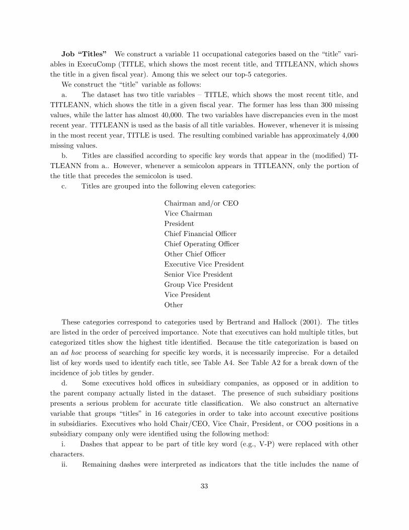
Job “Titles” We construct a variable 11 occupational categories based on the “title” vari-

ables in ExecuComp (TITLE, which shows the most recent title, and TITLEANN, which shows

the title in a given fiscal year). Among this we select our top-5 categories.

We construct the “title” variable as follows:

a. The dataset has two title variables – TITLE, which shows the most recent title, and

TITLEANN, which shows the title in a given fiscal year. The former has less than 300 missing

values, while the latter has almost 40,000. The two variables have discrepancies even in the most

recent year. TITLEANN is used as the basis of all title variables. However, whenever it is missing

in the most recent year, TITLE is used. The resulting combined variable has approximately 4,000

missing values.

b. Titles are classified according to specific key words that appear in the (modified) TI-

TLEANN from a.. However, whenever a semicolon appears in TITLEANN, only the portion of

the title that precedes the semicolon is used.

c. Titles are grouped into the following eleven categories:

Chairman and/or CEO

Vice Chairman

President

Chief Financial Officer

Chief Operating Officer

Other Chief Officer

Executive Vice President

Senior Vice President

Group Vice President

Vice President

Other

These categories correspond to categories used by Bertrand and Hallock (2001). The titles

are listed in the order of perceived importance. Note that executives can hold multiple titles, but

categorized titles show the highest title identified. Because the title categorization is based on

an ad hoc process of searching for specific key words, it is necessarily imprecise. For a detailed

list of key words used to identify each title, see Table A4. See Table A2 for a break down of the

incidence of job titles by gender.

d. Some executives hold offices in subsidiary companies, as opposed or in addition to

the parent company actually listed in the dataset. The presence of such subsidiary positions

presents a serious problem for accurate title classification. We also construct an alternative

variable that groups “titles” in 16 categories in order to take into account executive positions

in subsidiaries. Executives who hold Chair/CEO, Vice Chair, President, or COO positions in a

subsidiary company only were identified using the following method:

i. Dashes that appear to be part of title key word (e.g., V-P) were replaced with other

characters.

ii. Remaining dashes were interpreted as indicators that the title includes the name of

33

the subsidiary company. Above-mentioned titles were then reclassified as subsidiary titles, e.g.,

President sub.

The results of the analysis do not change when we use this alternative definition for job “titles.”

e. It should be noted that there are also instances of shared positions, e.g., Co-CEOs. In

all classifications the “co-“ prefix is ignored and such executives are treated like full CEOs, etc.

There are also instances of multiple executives within a firm and year with the same title. Again,

no special treatment is given to such observations.

The results of our regression analysis do not change when we use this alternative definition of

job “titles.” Hence, we do not report them in the paper.

A.3 Summary statistics

Table 10: Summary statistics by sample

Full sample Female Male

Mean Std.Dev. N Mean Std.Dev. N

Market value 9,278 23,928 1,581 8,651 26,032 43,746Assets 18,711 92,203 1,590 15,992 67,856 43,945

Age sample Female Male

Mean Std.Dev. N Mean Std.Dev. N

Market value 7,587 19,504 784 8,400 26,674 31,537Assets 12,370 68,277 791 15,058 65,454 31,679Age 47.63 6.968 791 53.69 8.437 31,685

Notes: See Table 1 for variable definitions and data sources.Market value and assets are expressed in constant,year 2000 US$.

34

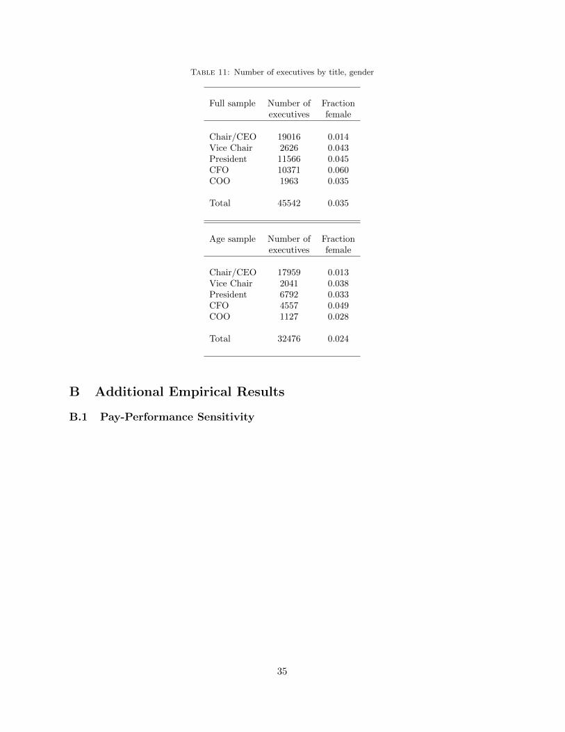
Table 11: Number of executives by title, gender

Full sample Number of Fractionexecutives female

Chair/CEO 19016 0.014Vice Chair 2626 0.043President 11566 0.045CFO 10371 0.060COO 1963 0.035

Total 45542 0.035

Age sample Number of Fractionexecutives female

Chair/CEO 17959 0.013Vice Chair 2041 0.038President 6792 0.033CFO 4557 0.049COO 1127 0.028

Total 32476 0.024

B Additional Empirical Results

B.1 Pay-Performance Sensitivity

35

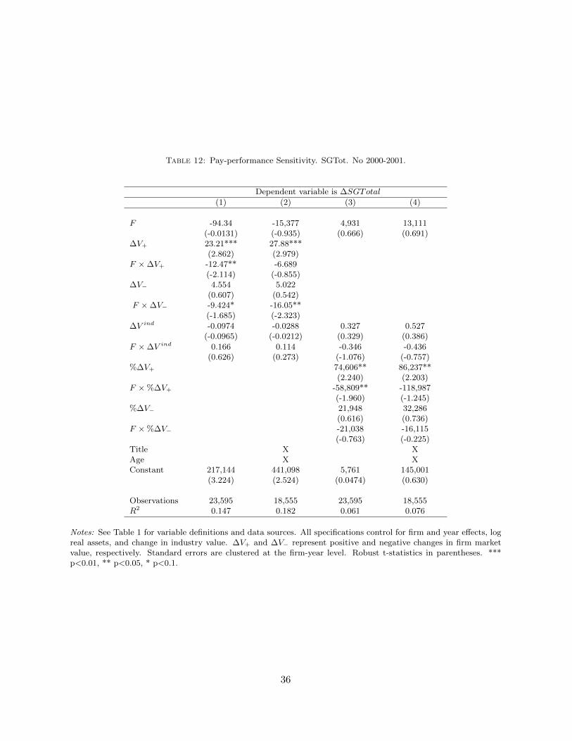
Table 12: Pay-performance Sensitivity. SGTot. No 2000-2001.

Dependent variable is ∆SGTotal

(1) (2) (3) (4)

F -94.34 -15,377 4,931 13,111(-0.0131) (-0.935) (0.666) (0.691)

∆V+ 23.21*** 27.88***(2.862) (2.979)

F × ∆V+ -12.47** -6.689(-2.114) (-0.855)

∆V− 4.554 5.022(0.607) (0.542)

F × ∆V− -9.424* -16.05**(-1.685) (-2.323)

∆V ind -0.0974 -0.0288 0.327 0.527(-0.0965) (-0.0212) (0.329) (0.386)

F × ∆V ind 0.166 0.114 -0.346 -0.436(0.626) (0.273) (-1.076) (-0.757)

%∆V+ 74,606** 86,237**(2.240) (2.203)

F × %∆V+ -58,809** -118,987(-1.960) (-1.245)

%∆V− 21,948 32,286(0.616) (0.736)

F × %∆V− -21,038 -16,115(-0.763) (-0.225)

Title X XAge X XConstant 217,144 441,098 5,761 145,001

(3.224) (2.524) (0.0474) (0.630)

Observations 23,595 18,555 23,595 18,555R2 0.147 0.182 0.061 0.076

Notes: See Table 1 for variable definitions and data sources. All specifications control for firm and year effects, logreal assets, and change in industry value. ∆V+ and ∆V− represent positive and negative changes in firm marketvalue, respectively. Standard errors are clustered at the firm-year level. Robust t-statistics in parentheses. ***p<0.01, ** p<0.05, * p<0.1.

36

Table 13: Pay Performance Sensitivity. Positive Changes in Market Value. SG Total

Dependent variable is ∆SGTotal(1) (2) (3) (4) (5) (6) (7) (8)

F 14,491* 5,993 11,093 -596.0 11,562* 18,195 9,871 15,509(7,907) (14,535) (7,222) (13,996) (6,509) (11,393) (6,431) (11,636)

∆V+ 23.01*** 26.83*** 23.33*** 27.23***(7.141) (8.428) (7.225) (8.533)

F ×∆V+ -12.34** -6.549 -14.52** -7.268(5.572) (7.583) (5.720) (10.39)

FCEO 26,444** 32,616** 12,405** 8,398(10,901) (14,028) (5,279) (7,646)

FCEO ×∆V+ -15.33*** -18.05***(5.364) (6.418)

F × FCEO ×∆V+ 21.07*** 14.81(6.691) (10.83)

%∆V+ 63,115*** 75,710*** 63,249*** 75,794***(23,390) (28,116) (23,466) (28,192)

F ×%∆V+ -56,711** -103,408 -62,305** -120,395(23,721) (65,477) (25,540) (80,065)

FCEO ×%∆V+ -35,257* -35,319(21,242) (25,930)

F × FCEO ×%∆V+ 61,720* 112,340(32,149) (79,828)

Title X X X XAge X X X XConstant 340,865*** 601,499*** 335,971*** 591,523*** 121,358 289,677 120,907 290,752

(74,079) (175,611) (73,776) (175,044) (105,062) (200,207) (105,233) (200,460)

Observations 28,257 22,266 28,257 22,266 28,257 22,266 28,257 22,266R2 0.092 0.110 0.093 0.112 0.020 0.026 0.020 0.026

Notes: See Table 1 for variable definitions and data sources. All specifications control for firm and year effects, logreal assets, and change in industry value. ∆V+ represents positive changes in firm market value. Standard errorsare clustered at the firm-year level. Robust t-statistics in parentheses. *** p<0.01, ** p<0.05, * p<0.1

37

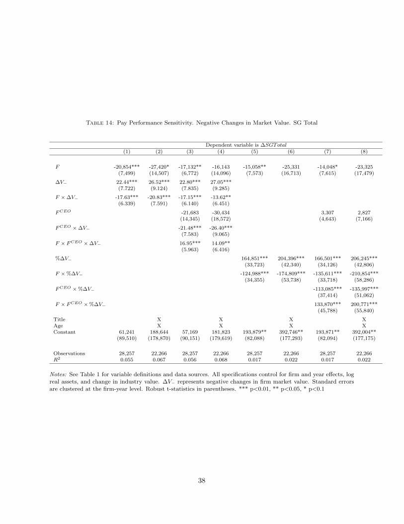
Table 14: Pay Performance Sensitivity. Negative Changes in Market Value. SG Total

Dependent variable is ∆SGTotal(1) (2) (3) (4) (5) (6) (7) (8)

F -20,854*** -27,420* -17,132** -16,143 -15,058** -25,331 -14,048* -23,325(7,499) (14,507) (6,772) (14,096) (7,573) (16,713) (7,615) (17,479)

∆V− 22.44*** 26.52*** 22.80*** 27.05***(7.722) (9.124) (7.835) (9.285)

F ×∆V− -17.63*** -20.83*** -17.15*** -13.62**(6.339) (7.591) (6.140) (6.451)

FCEO -21,683 -30,434 3,307 2,827(14,345) (18,572) (4,643) (7,166)

FCEO ×∆V− -21.48*** -26.40***(7.583) (9.065)

F × FCEO ×∆V− 16.95*** 14.09**(5.963) (6.416)

%∆V− 164,851*** 204,396*** 166,501*** 206,245***(33,723) (42,340) (34,126) (42,806)

F ×%∆V− -124,988*** -174,809*** -135,611*** -210,854***(34,355) (53,738) (33,718) (58,286)

FCEO ×%∆V− -113,085*** -135,997***(37,414) (51,062)

F × FCEO ×%∆V− 133,870*** 200,771***(45,788) (55,840)

Title X X X XAge X X X XConstant 61,241 188,644 57,169 181,823 193,879** 392,746** 193,871** 392,004**

(89,510) (178,870) (90,151) (179,619) (82,088) (177,293) (82,094) (177,175)

Observations 28,257 22,266 28,257 22,266 28,257 22,266 28,257 22,266R2 0.055 0.067 0.056 0.068 0.017 0.022 0.017 0.022

Notes: See Table 1 for variable definitions and data sources. All specifications control for firm and year effects, logreal assets, and change in industry value. ∆V− represents negative changes in firm market value. Standard errorsare clustered at the firm-year level. Robust t-statistics in parentheses. *** p<0.01, ** p<0.05, * p<0.1

38

B.2 Evidence from ATUS

39

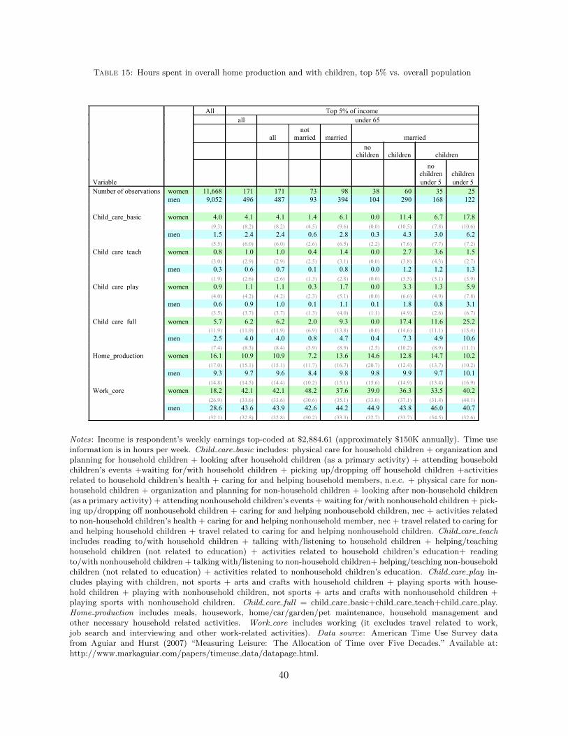
Table 15: Hours spent in overall home production and with children, top 5% vs. overall population

All Top 5% of income all under 65

all not

married married married

no

children children children

Variable

no children under 5

children under 5

Number of observations women 11,668 171 171 73 98 38 60 35 25 men 9,052 496 487 93 394 104 290 168 122 Child_care_basic women 4.0 4.1 4.1 1.4 6.1 0.0 11.4 6.7 17.8 (9.3) (8.2) (8.2) (4.5) (9.6) (0.0) (10.5) (7.8) (10.6) men 1.5 2.4 2.4 0.6 2.8 0.3 4.3 3.0 6.2 (5.5) (6.0) (6.0) (2.6) (6.5) (2.2) (7.6) (7.7) (7.2) Child_care_teach women 0.8 1.0 1.0 0.4 1.4 0.0 2.7 3.6 1.5 (3.0) (2.9) (2.9) (2.5) (3.1) (0.0) (3.8) (4.3) (2.7) men 0.3 0.6 0.7 0.1 0.8 0.0 1.2 1.2 1.3 (1.9) (2.6) (2.6) (1.3) (2.8) (0.0) (3.5) (3.1) (3.9) Child_care_play women 0.9 1.1 1.1 0.3 1.7 0.0 3.3 1.3 5.9 (4.0) (4.2) (4.2) (2.3) (5.1) (0.0) (6.6) (4.9) (7.8) men 0.6 0.9 1.0 0.1 1.1 0.1 1.8 0.8 3.1 (3.5) (3.7) (3.7) (1.3) (4.0) (1.1) (4.9) (2.6) (6.7)

Child_care_full women 5.7 6.2 6.2 2.0 9.3 0.0 17.4 11.6 25.2 (11.9) (11.9) (11.9) (6.9) (13.8) (0.0) (14.6) (11.1) (15.4) men 2.5 4.0 4.0 0.8 4.7 0.4 7.3 4.9 10.6 (7.4) (8.3) (8.4) (3.9) (8.9) (2.5) (10.2) (8.9) (11.1) Home_production women 16.1 10.9 10.9 7.2 13.6 14.6 12.8 14.7 10.2 (17.0) (15.1) (15.1) (11.7) (16.7) (20.7) (12.4) (13.7) (10.2) men 9.3 9.7 9.6 8.4 9.8 9.8 9.9 9.7 10.1 (14.8) (14.5) (14.4) (10.2) (15.1) (15.6) (14.9) (13.4) (16.9) Work_core women 18.2 42.1 42.1 48.2 37.6 39.0 36.3 33.5 40.2 (26.9) (33.6) (33.6) (30.6) (35.1) (33.0) (37.1) (31.4) (44.1) men 28.6 43.6 43.9 42.6 44.2 44.9 43.8 46.0 40.7 (32.1) (32.8) (32.8) (30.2) (33.3) (32.7) (33.7) (34.5) (32.6)

Notes: Income is respondent’s weekly earnings top-coded at $2,884.61 (approximately $150K annually). Time useinformation is in hours per week. Child care basic includes: physical care for household children + organization andplanning for household children + looking after household children (as a primary activity) + attending householdchildren’s events +waiting for/with household children + picking up/dropping off household children +activitiesrelated to household children’s health + caring for and helping household members, n.e.c. + physical care for non-household children + organization and planning for non-household children + looking after non-household children(as a primary activity) + attending nonhousehold children’s events + waiting for/with nonhousehold children + pick-ing up/dropping off nonhousehold children + caring for and helping nonhousehold children, nec + activities relatedto non-household children’s health + caring for and helping nonhousehold member, nec + travel related to caring forand helping household children + travel related to caring for and helping nonhousehold children. Child care teachincludes reading to/with household children + talking with/listening to household children + helping/teachinghousehold children (not related to education) + activities related to household children’s education+ readingto/with nonhousehold children + talking with/listening to non-household children+ helping/teaching non-householdchildren (not related to education) + activities related to nonhousehold children’s education. Child care play in-cludes playing with children, not sports + arts and crafts with household children + playing sports with house-hold children + playing with nonhousehold children, not sports + arts and crafts with nonhousehold children +playing sports with nonhousehold children. Child care full = child care basic+child care teach+child care play.Home production includes meals, housework, home/car/garden/pet maintenance, household management andother necessary household related activities. Work core includes working (it excludes travel related to work,job search and interviewing and other work-related activities). Data source: American Time Use Survey datafrom Aguiar and Hurst (2007) “Measuring Leisure: The Allocation of Time over Five Decades.” Available at:http://www.markaguiar.com/papers/timeuse data/datapage.html.

40

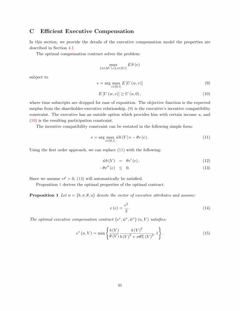
C Efficient Executive Compensation

In this section, we provide the details of the executive compensation model the properties are

described in Section 4.1

The optimal compensation contract solves the problem:

maxw(∆V ),e,e∈[0,1]

ES (e)

subject to

e = arg maxe∈[0,1]

E [U (w, e)] (9)

E [U (w, e)] ≥ U (u, 0) , (10)

where time subscripts are dropped for ease of exposition. The objective function is the expected

surplus from the shareholder-executive relationship, (9) is the executive’s incentive compatibility

constraint. The executive has an outside option which provides him with certain income u, and

(10) is the resulting participation constraint.

The incentive compatibility constraint can be restated in the following simple form:

e = arg maxe∈[0,1]

wb (V ) e− θv (e) . (11)

Using the first order approach, we can replace (11) with the following:

wb (V ) = θv′ (e) , (12)

−θv′′ (e) ≤ 0. (13)

Since we assume v′′ > 0, (13) will automatically be satisfied.

Proposition 1 derives the optimal properties of the optimal contract.

Proposition 1 Let n = b, σ, θ, u denote the vector of executive attributes and assume:

v (e) =e2

2. (14)

The optimal executive compensation contract e∗, w∗, w∗ (n, V ) satisfies:

e∗ (n, V ) = min

b (V )

θ (V )

b (V )2

b (V )2 + σθΣ (V )2 , 1

. (15)

41

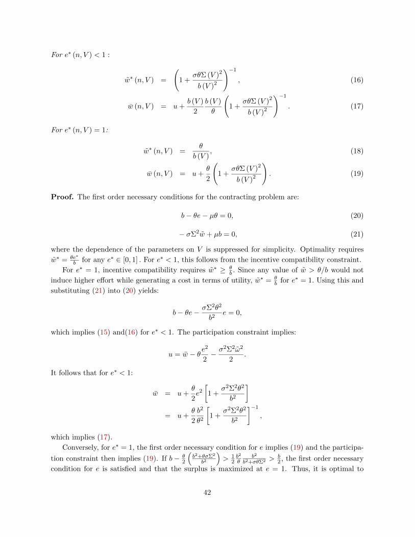
For e∗ (n, V ) < 1 :

w∗ (n, V ) =

(1 +

σθΣ (V )2

b (V )2

)−1

, (16)

w (n, V ) = u+b (V )

2

b (V )

θ

(1 +

σθΣ (V )2

b (V )2

)−1

. (17)

For e∗ (n, V ) = 1:

w∗ (n, V ) =θ

b (V ), (18)

w (n, V ) = u+θ

2

(1 +

σθΣ (V )2

b (V )2

). (19)

Proof. The first order necessary conditions for the contracting problem are:

b− θe− µθ = 0, (20)

− σΣ2w + µb = 0, (21)

where the dependence of the parameters on V is suppressed for simplicity. Optimality requires

w∗ = θe∗

b for any e∗ ∈ [0, 1] . For e∗ < 1, this follows from the incentive compatibility constraint.

For e∗ = 1, incentive compatibility requires w∗ ≥ θb . Since any value of w > θ/b would not

induce higher effort while generating a cost in terms of utility, w∗ = θb for e∗ = 1. Using this and

substituting (21) into (20) yields:

b− θe− σΣ2θ2

b2e = 0,

which implies (15) and(16) for e∗ < 1. The participation constraint implies:

u = w − θe2

2− σ2Σ2ω2

2.

It follows that for e∗ < 1:

w = u+θ

2e2

[1 +

σ2Σ2θ2

b2

]= u+

θ

2

b2

θ2

[1 +

σ2Σ2θ2

b2

]−1

,

which implies (17).

Conversely, for e∗ = 1, the first order necessary condition for e implies (19) and the participa-

tion constraint then implies (19). If b− θ2

(b2+θσΣ2

b2

)> 1

2b2

θb2

b2+σθΣ2 >b2 , the first order necessary

condition for e is satisfied and that the surplus is maximized at e = 1. Thus, it is optimal to

42

maximize effort.

Endogenous Size Distribution of Executives Let the distribution of n, the vector of ex-

ecutive attributes, be ϕi (·) for i = f,m, where f stands for female and m for male. Let Ni be

the support of the distribution. Then, we can derive the population wide probability distribution

density of n. Take an executive/firm pair: n, V and let, Ω, denote total market capitalization.

We now derive the solution of the optical assignment problem. Let n = b, σ, θ, u denote the

vector of executive attributes and let the distribution of n in the population of executives be ϕi (·)for i = f,m, where f stands for female and m for male. Let Ni be the support of the distribution.

The population wide probability distribution density of n, denoted with ϕ (·), is defined over the

support Nf ∪Nm. For example, if only one characteristic in n varies by gender and ϕi is a uniform

and Ni = [ni, ni] with nm > nf and nf < nm, then:

Pr (n ≤ n) = πf

∫ maxn,nf

minn,nf1

nf − nfdx+ πm

∫ maxn,nm

minn,nm

1

nm − nmdx,

where πi i = f,m is the fraction of executives on gender i in the population.

Take an executive/firm pair n, V , and let Ω denote total market capitalization. The optimal

firm size distribution maximizes economy wide surplus:

maxV (n)≥0

∫Nf∪Nm

S∗ (n, V (n))ϕ (n) dn,

subject to

Ω =

∫Nf∪Nm

V (n)ϕ (V ) dV. (22)

By Proposition 1, the maximized surplus from the firm-executive relationship is:

S∗ (n, V ) =

b(V )

2b(V )θ

(1 + σθΣ(V )2

b(V )2

)−1for e∗ < 1,

b (V )− θ2

(1 + σθΣ(V )2

b(V )2

)for e∗ = 1.

(23)

We will assume that the attributes are ranked so that the top end of the support corresponds

to the combination of attributes that maximizes the surplus absent any incentive problems, and

denote that attribute with n.

The solution to the assignment problem is characterized in the following proposition.

Proposition 2 The optimal size distribution of executives satisfies:

V (n) = (b (n))− 1

(2γ−1)

1

2

∫ nn (b (n))

−1(2γ−1) ϕ (n) dn

Ω

−1

(24)

43

for e∗(n) < 1 and

V (n) =

0 for n < n

Ω forn = n(25)

for e∗(n) = 1.

Proof. The envelope condition for the optimal contracting problem is:

S∗V = γS∗

V. (26)

Then, the first order condition for the assignment problem is:

S∗V (n, V (n))ϕ (n)− ϕ (n) ζ

≤ 0

= 0 for V (n) > 0(27)

where ζ is the multiplier on constraint (22), jointly with (22).

For e∗ < 1, at an interior optimum, equation (27) implies:

γS∗ (n, V (n))

V (n)= ζ, (28)

which implies:

V (n) =

ζ

γ(V (n))−1

1/(2γ−1)

. (29)

Rearranging (28) and integrating over Nf ∪Nm, substitutions obtain the solution for ζ:

γ

∫Nf∪Nm

S∗ (n, V (n))ϕ (n) dn = ζ

∫Nf∪Nm

V (n)ϕ (n) dn,

γ

∫S∗ (n, V (n))ϕ (n) dn

Ω= ζ,

1

2

∫ nn (b (n))

−1(2γ−1) ϕ (n) dn

Ω=

(ζ

γ

) −1(2γ−1)

. (30)

Combining (29) and (30) obtains (24).

For e∗ = 1, from the first order condition (27), evaluated at e∗ = 1, assuming an interior

solution:

V =

[ζ

γb

] 1γ−1

(31)

for n < n, in order for the optimum to be interior. To solve for ζ, use equation (31) in (22), to

obtain:

ζ = bγΩγ−1.

Substituting this result in (31), yields: V = Ω. Second order conditions then imply that V (n) = Ω,

and the optimum is not interior. Hence, (25).

44