Embed Size (px)
Citation preview
GEM and PLEXOS in the SOO/GIT Process:
Conceptual Commentary
Prepared for
The New Zealand Electricity Commission
by
E Grant Read
Draft 1.9
16 November 2007
DISCLAIMER This document is supplied for the purposes of facilitating discussions with the client, and electricity sector participants. Neither the author(s) nor EGR Consulting Ltd,, make any representation or warranty as to the accuracy or completeness of this document, or accept any liability for any omissions, or for statements, opinions, information or matters arising out of, contained in or derived from this document, or related communications, or for any actions taken on such a basis.
EGR Consulting Ltd.
2
GEM / PLEXOS Comparison
Executive Summary 1. This report has been prepared at the request the New Zealand Electricity Commission (the
Commission) to assist them in understanding the implications of using either GEM, or the LT Plan module of PLEXOS for transmission planning studies in the SOO/GIT process. Specifically, we focus on the application of these two models to the upcoming submission with respect to an upgrade of the inter-island HVDC link.
2. The aim is not to produce a comprehensive review of either model, or to determine which is “better”. PLEXOS is clearly a more comprehensive modelling suite, and potentially more versatile and more accurate as a result. But complexity does not necessarily produce accuracy, and we believe it to be desirable that issues of this nature be examined using (at least) two different modelling approaches. Thus we consider that GEM also has a useful role to play, and consider options for further development of GEM so as to better fulfil that role in future.
3. Broad consideration of the situation,, and of the nature of MILP modelling, leads us to stress:
• The desirability of keeping computational requirements down to a level which allows for a practical and timely analytical and decision-making process to be conducted.
• The fact that adding complexity to models does not necessarily improve the quality of their recommendations, particularly if that complexity is added to a different module of the modelling system than the one in which the key decisions are optimised.
• The desirability of increasing the credibility of model results, as market simulations, by minimising the gap between the model’s assessment of the “economic” investment, and/or investment market participants might reasonably make on a commercial basis, and investment “required” to meet any externally imposed capacity requirements.
4. More detailed discussions are developed under four broad headings:
• Modelling System Operations;
• Modelling Economic Investment;
• Modelling Capacity Adequacy; and
• Modelling Market Behaviour.
5. While PLEXOS can allow relatively detailed modelling of system operations, such modelling will always be approximate in a long term planning model, and it would be claiming spurious accuracy to pretend otherwise. What matters, even in a centrally planned environment, are the model’s internally calculated signals for investment in both generation and transmission capacity. Thus the value of operational modelling is largely measured by the credibility of the Price Duration Curve (PDC) it produces, and of inter-regional price differentials.
EGR Consulting Ltd Final Version 20/11/2007
3
GEM / PLEXOS Comparison 6. At a more detailed level, we suggest that:
• Given that the MILP optimisation is essentially deterministic, we see little point in modelling operational decision periods shorter than one quarter.
• Since spinning reserve in important in the New Zealand system, and may affect the economics of HVDC investment, it should really be modelled explicitly, as it is in PLEXOS, but not in GEM.
• The expected load variability represented by the LDC should be augmented by consideration of variability due to unit breakdowns, wind, tributary flows and (short term) load uncertainty.
• Because the variability of hydro inflows has such a significant impact on the generation capacity mix required by the New Zealand system, it really should be accounted for in the optimisation of capacity investment, not just in subsequent simulation of system operation.
• Modelling of hydro storage and river chain management is an important issue, and PLEXOS does provide reasonable facilities to perform a plausible endogenous optimisation, even if some aspects of that model may benefit from further tuning.
• Rather than introduce similar complexity into GEM, though, the current approach, in which another model is used to pre-compute a set of hydro output schedules for different hydrology years, could be developed further.
7. By “economic” investment we mean the least cost investment plan to meet load and/or spinning reserve requirements, from a national cost benefit perspective, under a particular scenario. We consider that the analytical process should be structured so that each MILP optimisation relates to the optimisation of generation capacity investment and performance for a particular scenario, under some fixed assumption with respect to HVDC investment. That is, we aim to find a single HVDC decision which is optimal over all scenarios, not an optimal HVDC decision for each scenario.
8. At a more detailed level, we conclude that:
• Integer variables should probably only be used for modelling some larger generation projects, in the more immediate future, particularly if they interact significantly with the transmission options under consideration.
• The use of integer variables, in combination with capacity constraints may lead the model to predict extended periods in which simulated energy prices are insufficient to cover the costs of the recommended entry without introducing a capacity pricing component.
• In principle, plant retirement should really be optimised along with the plant investment variables, but this would involve introducing a more complex formulation, and is probably only worthwhile for a small set of key plant.
• Generation/transmission interactions are adequately modelled by the standard formulation. But co-optimisation of the HVDC decision with generation expansion, while possible, is not recommended for other reasons.
EGR Consulting Ltd Final Version 20/11/2007
4
GEM / PLEXOS Comparison • The interaction between old and new hydro developments on the same river system
may be better modelled using an exogenous model such as SDDP to pre-compute alternative datasets, summarising performance with and without key developments.
• The interaction between investment in less reliable generation types, such as wind, and the Effective LDC (ELDC) faced by the remainder of the sector could be modelled by pre-computing incremental contributions to the ELDC, then allowing the MILP to interpolate as a function of cumulative build.
• In the case of wind it may also be appropriate to model its influence on spinning reserve requirements and/or to create a constraint specifying a requirement for a new “standby” ancillary service designed to cope with its particular characteristics.
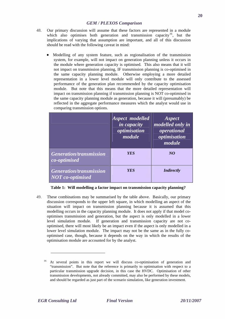
9. The modelling of “Capacity Adequacy” relates to additional constraints designed to ensure that sufficient plant is built to meet some externally specified capacity requirements, even if the model does not consider that investment to be the most “economic” response to the range of supply/demand situations it has been asked to cover. Even so, the model can still minimise the cost of meeting these requirements from a national cost benefit perspective and, from that perspective, it should do so in a single optimisation, covering both “capacity” driven and “economic” investment.
10. In particular we suggest that:
• The apparent need for additional capacity should be minimised, as far as possible by accurate modelling of requirements to cover spinning reserve, dry year backup, unit breakdowns etc.
• The Augmented LDC (ALDC) concept provides a mechanism to do this, with shortage costs adjusted so as to ensure that capacity requirements are given appropriate weight for investment purposes.
• The meeting of dry year backup requirements should be treated by optimisation of investment and operations over the entire range of hydrologies simultaneously, rather than just for a single dry year.
11. All of the above relates to the use of MILP to optimise decisions from a national cost benefit perspective, but further complications arise with respect to the modelling of market behaviour. If the goal is supposed to be realistic market simulation, then commercial incentives should be modelled, if possible. Modelling deviations from national cost benefit optimisation is difficult in a MILP framework, but there is no better framework immediately available.
12. More specifically, we conclude that:
• Because the HVDC cost recovery rule is not consistent with national cost benefit optimisation, its impact can not be modelled in a model which also optimises HVDC investment. Thus each optimisation run should assume a specified HVDC investment as occurring at a specified date.
• Unfortunately the cost recovery rule also implies different incentives for different parties, but the formula proposed for implementation in PLEXOS seems appropriate, at a first order level, provided we can identify particular projects with particular participants.
EGR Consulting Ltd Final Version 20/11/2007

5
GEM / PLEXOS Comparison • Including capacity requirement constraints in an integrated optimisation of
generation investment implicitly would simulate a market in which payments are made for capacity, as well as energy and spinning reserve. Thus we should not expect the energy (and spinning reserve) prices alone to be high enough to sustain the projected entry.
• Rather than the integrated national cost benefit optimisation approach recommended in Section 5.3, a two-phase approach may have to be maintained in order to simulate the effect of current policies under which the Commission may intervene to build extra peaking capacity if the market does not.
• In principle, we consider that generator gaming should be modelled. But this is difficult in a MILP framework, and experience to date suggests that it brings limited benefit, in terms of assessing the value of transmission investment. Still, PLEXOS may make a useful contribution in this regard, at least as a sensitivity.
• An alternative interpretation of the results from MILP optimisation involving capacity constraints is that participants will be allowed to cover the revenue gap caused by the absence of a capacity market by gaming prices up to levels high enough to cover the cost of plant entering to meet capacity requirements. But so long as policy on such matters remains unclear, the realism of any market simulations will also remain unclear.
EGR Consulting Ltd Final Version 20/11/2007
6
GEM / PLEXOS Comparison
Contents
1. Introduction 9
2. Modelling in the SOO/GIT Process 13
2.1. The Situation 13
2.2. The Nature of MILP Modelling 14
2.3. Practicality 16
2.4. Stochastic vs Probabilistic Modelling 17
2.5. Structure of Modelling Systems 19
2.6. Credibility 24
3. Modelling System Operations 27
3.1. Overview 27
3.2. Chronological vs LDC Modelling 30
3.3. Real Time Issues 32
3.3.1. Transmission 32
3.3.2. Spinning Reserve 35
3.3.3. Load Variability 40
3.3.4. Supply Side Uncertainty 41
3.4. Short Term Issues 45
3.4.1. Minimum Running Limits 45
3.4.2. Short Term Energy Limits 47
3.4.3. River Chains 47
3.4.4. Inflexible Thermal Plant 50
EGR Consulting Ltd Final Version 20/11/2007
7
GEM / PLEXOS Comparison
3.5. Mid-Term Issues 51
3.5.1. Modelling Hydrological Uncertainty 51
3.5.2. Modelling Reservoir Management 54
3.5.3. Annual Energy Limits 63
4. Modelling Economic Investment 65
4.1. Overview 65
4.2. Dealing with Alternative Scenarios 66
4.3. Use of Integer Variables 69
4.3.1. Impact of Load Forecasting Errors 70
4.3.2. Impact of Cost Forecasting Errors 72
4.3.3. Impact of LDC Variation 72
4.3.4. Load Growth Rate and Scale Economies 73
4.3.5. Impact of the Transmission System 74
4.3.6. Implications for Transmission Planning 75
4.3.7. Pricing Implications 78
4.4. Modelling Plant Retirement 80
4.5. Modelling Investment Dependencies 83
4.5.1. Transmission vs Generation 83
4.5.2. Old vs new Hydro 84
4.5.3. Investment and ELDC Variability 86
4.5.4. Wind vs Reserve Requirements 88
5. Modelling Capacity Adequacy 90
5.1. Overview 90
5.2. Modelling “Non-Supply” 91
5.3. Modelling Capacity Constraints 93
EGR Consulting Ltd Final Version 20/11/2007
8
GEM / PLEXOS Comparison
6. Modelling Market Behaviour 101
6.1. Overview 101
6.2. Commercial Objectives 102
6.3. Transmission Investment and Cost Recovery 107
6.3.1. Cost recovery with co-optimisation 108
6.3.2. Cost recovery without co-optimisation 111
6.3.3. Implementation using GEM/PLEXOS 118
6.4. Market Implications of Capacity Requirement Modelling 119
6.5. The Impact of Generator Gaming 125
EGR Consulting Ltd Final Version 20/11/2007
9
GEM / PLEXOS Comparison
GEM and PLEXOS in the SOO/GIT Process
1. Introduction 1. This report has been prepared at the request the New Zealand Electricity Commission (the
Commission) by EGR Consulting Ltd. It draws, in part, on a preliminary review of the Generation Expansion Model (GEM,) previously prepared for Meridian Energy Limited (MEL), and available on the Commission’s website.1 At that time, only limited documentation was available for review. In the meantime, GEM itself has been developed further, while we have been able to review further documentation,2 and have extensive discussions with Commission staff. Thus this review takes up the various issues raised in our earlier review, along with some related matters, and comes to more definite conclusions with respect to the way in which GEM, as now configured, actually deals with those issues, and how it might be modified to do so better.
2. Our earlier review focussed on the use of GEM by the Commission to support the development of scenarios to be employed in the transmission planning process. These scenarios are intended to represent alternative futures for the New Zealand electricity sector, over a long planning horizon. They are to be incorporated into a Statement of Opportunities (SOO) upon which Transpower is supposed to base its submissions with respect to the application of the Grid Investment Test (GIT) to any proposed Grid Upgrade Plan (GUP).
3. But the transmission planning process also requires Transpower to undertake modelling in order to support its case that a particular transmission development proposal satisfies the GIT. We understand that Transpower intends to use GEM for that purpose, too, at least in the initial stages of evaluating its current HVDC proposals. The issues here are slightly different, because transmission is being optimised, and possibly co-optimised with generation. Thus, at times, we will need to comment on the two cases separately.
4. We also understand that Transpower intends to supplement its GEM analyses with more detailed analyses undertaken using a new LT Plan module, recently developed as part of the PLEXOS modelling system3. McLennan Magasanik Associates (MMA) are assisting Transpower, by implementing a formulation of the New Zealand generation/transmission expansion optimisation, using LT Plan, and have documented
1 Using GEM to produce SOO Scenario: A Preliminary Conceptual Critique. EGR
Consulting report to Meridian Energy Ltd. See http://www.electricitycommission.govt.nz/opdev/modelling/gem/documentation.
2 In particular see GEM: An explanation of the equations in version 1.2.0 at http://www.electricitycommission.govt.nz/opdev/modelling/gem/documentation.
3 Produced by Energy Exemplar (EE) see http://www.plexos.info/wiki/
EGR Consulting Ltd Final Version 20/11/2007

10
GEM / PLEXOS Comparison
that module in relation to its application to this particular problem situation4 Thus we have also been asked to compare and contrast the GEM and PLEXOS models for this purpose.
5. Since documentation of both models is now available from their respective authors, we will not attempt to summarise the models ourselves, and simply refer the reader to those documents.5 We note, though, that both models have been under continuous development during the course of this review, and we expect that will continue to be the case. Thus statements in this review should not be taken as authoritative statements of the state of model development, even at the time of writing, and may be expected to become progressively outdated, subsequently.6
6. Both GEM and PLEXOS incorporate a Mixed Integer Linear Programming (MILP) formulation of the capacity expansion problem. This type of model has traditionally been used for centralised generation/transmission expansion planning, and more recently to produce forecasts and scenario projections for decentralised planning purposes. It will be noted that MILP is not ideal for the latter purpose, and there are models better suited to looking at particular aspects of the problem.7 But, in our view, there is no better comprehensive modelling framework readily available to the Commission, or to Transpower, at this time. Thus, with some caveats, we endorse the application of a MILP approach in this context, and at this time. Options for development of radically different approaches will be considered at a later date.
7. Our previous report commented, primarily, on general issues which arise with the application of MILP modelling to this kind of situation, and only secondarily alluded to the implications which these observations could have for the way in which we understood GEM to have been applied in producing SOO scenarios. Our comments related to three broad areas:
a) The intended role of SOO scenarios;
b) The use of MILP as a capacity optimisation methodology in a centralised planning environment; and
c) The use of MILP as a market forecasting methodology.
8. Conversely, there were a large number of issues on which we made little or no comment, including:
4 Capacity Expansion Planning for the New Zealand Electricity Market, MMA report to
Transpower, v 4.2, October 3, 2007. 5 See references above. 6 Also, while comments made here are reliant, in part, on discussions with both Commission
staff and EE/MMA, all errors and omissions remain the responsibility of the author. 7 Including Cournot models of short term participant behaviour, for example, which are
available in various modelling systems, including PLEXOS, and CRA’s PEPPY modelling system used to assess “Competition Benefits” from upgrades to the North Island transmission system in Transpower's GIT application for the 400KV upgrade.
EGR Consulting Ltd Final Version 20/11/2007
11
GEM / PLEXOS Comparison
a) The ways in which the SOO scenarios were differentiated, or input assumptions differentiated between scenarios;
b) The assumptions made about load growth, or the costs of investment, production, or non-supply;
c) The plausibility of the SOO scenarios actually produced;
d) The likely computational efficiency of the GEM model; or
e) Details affecting the accuracy of the GEM model formulation.
9. Thus we did not come to any firm conclusions with respect to the suitability of GEM as a MILP Model of the New Zealand electricity sector. This report comes to firmer conclusions with respect to both GEM and PLEXOS. But it still does not address any of the issues listed above. In particular it does not comment in any way on the implementation of GEM or PLEXOS as pieces of software. PLEXOS, in particular, is a complex and comprehensive modelling system, many features of which are not directly relevant to the current application. Thus we should make it clear that, in discussing the “PLEXOS model” being employed in this context, we are not commenting on the “PLEXOS modelling system, nor even necessarily on the LT Plan module being employed for this analysis, but only on the specific formulation being proposed for GIT analysis by Transpower, as documented by MMA for this purpose.8
10. We should also make it clear that we have not studied the numerical input to, or output from, the scenario generation process. Thus all comment in this paper relates to matters of principle, without implying any judgment about the materiality of the effects discussed, in terms of their impact on the SOO scenarios, or on decisions with respect to transmission investment projects likely to be submitted for consideration in the next GIT application.
11. Our focus is, firstly, on the general form which this kind of model must take in order to fulfil its desired function, and hence indirectly on the form and nature of the required inputs and outputs. As in our previous report:
• We begin by reviewing the intended role of modelling in the SOO/GIT process.
• We then move on to consider various issues with respect to the use of MILP in a centrally planned environment, and
• Finally we consider the adaptation, and limitations, of MILP as a tool for forecasting market behaviour.
12. While either modelling system could be used for other purposes, this review focuses solely on the application of GEM and PLEXOS in the SOO/GIT process, as required to justify a transmission expansion proposal to the New Zealand Electricity Commission. In each section, we comment on the extent to which both GEM and PLEXOS can provide the modelling requirements of the SOO/GIT planning process.
8 See above, and also: PLEXOS New Zealand Database Assumptions Report MMA report to
Transpower, v 4.4, November 5, 2007.
EGR Consulting Ltd Final Version 20/11/2007

12
GEM / PLEXOS Comparison And since we recognise that perfection will not be attainable in this regard, we also comment on:
• How the various strengths and weaknesses of these models may complement each other;
• How the inevitable deficiencies in analysis may be taken into account in the decision-making process;
• How each model might be further developed; and
• How the level of accuracy and detail pursued in various areas may be balanced so as to provide the best value within the limited computational and analytical resources.
13. At various points we make suggestions about alternative ways in which various aspects of the problem could be modelled. In some cases these may be regarded as both innovative and untried. Obviously, such suggestions have not been thoroughly reviewed or tested in the context of this brief review, and so they should be regarded as tentative hypotheses to be tested both theoretically and experimentally.
14. Obviously, too, many of the “recommendations” advanced here could not be implemented in the timeframe necessary to expedite analysis of the upcoming GIT application, and should be seen as suggestions for longer term development. While we focus on the intended application of both models in assessing the merits of a proposed upgrade to the inter-island HVDC link, and this provides a useful conceptual case for consideration, some of these ideas would have to be adapted for application o other projects, in future years. The implications of this requirement would need to be considered before making any significant commitment to adopting any of these approaches.
EGR Consulting Ltd Final Version 20/11/2007
13
GEM / PLEXOS Comparison
2. Modelling in the SOO/GIT Process
2.1. The Situation 15. This report, like our earlier one, is based on the understanding that SOO scenarios are
supposed to be realistic projections of the pattern of investment, and hence of operations, under differing assumptions about the macro environment. So long as the New Zealand electricity sector is expected to continue operating on a market basis, the SOO scenarios are, in principle, supposed to be projections of market-driven investment, market-driven operation, and market-driven demand response.
16. We consider it likely that “realistic” projections, particularly of the more distant future, will not necessarily meet current Government policy goals. Indeed we believe that plausible scenarios can be constructed under which it could become very difficult to do so. But it is our understanding that the Commission considers that the transmission system should be planned on the assumption that current policy objectives will be met, at least for the range of scenarios to be considered. One might argue that robust planning should really consider the ability of the system to cope with more extreme situations, but it is probably fair to conclude that a transmission system planned to serve a steadily growing load with reliable generation supply would also be able to cope with lower load growth, or less adequate generation. So this seems a reasonable planning basis for transmission.
17. Accepting that assumption implies the need to constrain all modelled scenario solutions to comply with current policy, though, and that has important implications. We have previously argued that projected “energy market revenues”, alone, will be less than that which might otherwise seem necessary to support projected entry, if security/ capacity constraints are imposed to meet policy objectives. We note that Commission staff have responded that means will be found to ensure revenue adequacy, including modification to the market design, if necessary.
18. Such a commitment may be taken to increase the plausibility of scenarios in which modelled energy market revenue seems inadequate. But, if it is accepted, the nature of the mechanisms which might be employed to achieve this goal becomes a significant issue, because those mechanisms affect the balance of plant types which might be built. And this will impact on the location of new construction, and hence on the need for transmission.
19. Specifically, we argued that a MILP model effectively simulates the impact of a “two part” market, with energy trading, as at present, supplemented by a market for capacity tickets, which may account for a significant proportion of total market value.9
9 Although such markets may relate to what is often called “reserve capacity” in the
international literature, this is a separate issue from the need to provide “spinning reserve”. The latter is already provided for in the New Zealand market, which thus should not strictly be called an “energy only” market, and the implications of this are discussed in a later section.
EGR Consulting Ltd Final Version 20/11/2007
14
GEM / PLEXOS Comparison
20. Depending on how such a mechanism is implemented, it may favour investment in OCGT plant, for example, and this will presumably be reflected in model solutions. Thus, if other mechanisms are contemplated, consideration should be given to the ways in which real market outcomes may vary from market scenarios derived under that implicit assumption. This issue is re-visited in a later section, but it also has direct implications for the kind of modelling which should employed.
21. Finally, we note that, to date, GEM has only been used to prepare SOO scenarios, driven by alternative “world-views” with respect to the environment within which both generation and transmission development will occur.10 In that context, variations in load growth rates are not considered, and transmission development is not optimised. Application of the GIT requires a further step in the analysis, which is to optimise the configuration and timing of transmission network development, while considering a range of possible load growth rates.
22. Thus we must now extend our earlier discussion, which related primarily to the optimisation of generation development given an assumed pattern of transmission development, to cover the case in which transmission and generation are “co-optimised”. And we must consider the implications of using load growth sub-scenarios, and particularly the interpretation of model results derived assuming such a limited model of possible variation, in a real-world situation where load growth rates may be highly uncertain, and vary continuously.
2.2. The Nature of MILP Modelling 23. Both the GEM and PLEXOS modelling systems use more than one optimisation
model to optimise operation of, and/or investment in, (hypothetical) generation and/or transmission systems for future scenarios. Both rely heavily on MILP to solve these optimisation models, and the implications of employing that technique are explored extensively in this report.
24. A MILP model employs “Mixed Integer Linear Programming”. That is, it contains a mixture of integer and (continuous) linear components, and may be thought of as a Linear Program (LP) in which some variables have been restricted to take only integer values11. Alternatively, the integer variables can be thought of as defining a “tree”,12 each terminal node of which defines an LP, which to be solved with a particular combination of the integer variables fixed. This kind of structure allows optimal solutions to be found to problems which do have obvious integer variables (eg for capacity investment), but can also be applied to solve more general dis-continuous and/or non-convex problems (involving scale economies, for example).
10 At times we will refer to these as “world-view scenarios”, so as to distinguish them from
other, more detailed, (sub-) scenarios which may need to be considered in the context, for example, of stochastic optimisation of system operations.
11 Many MILP models use only “Binary” variables, restricted to be either 0 or 1, but this is not a general requirement.
12 The classic “Branch and bound” MILP solution algorithm effectively alternates between LP solutions corresponding to these two concepts.
EGR Consulting Ltd Final Version 20/11/2007

15
GEM / PLEXOS Comparison
le, at present.
25. MILP models have long been used for integrated centralised generation/transmission planning in the electricity sector. Such models can determine an optimal expansion plan. But optimality is only guaranteed under the assumptions implicit in the modelling technique, and formulation. Thus MILP models do have limitations, even in a centralised context.
26. Traditionally, the greatest limitation of MILP modelling has been that the computation time required to solve such models means that significant compromises must be made with respect to the level of detail with which various aspects of system behaviour can be modelled, and particularly with respect to the extent to which uncertainty can be modelled. This becomes particularly important in hydro systems, both because of the pervasive impact of hydrological uncertainty, and because of the (limited) ways in which hydro storage allows load variation, and uncertainty, to be managed.
27. The impact which the various approximations employed may have on model outcomes, and hence ultimately on transmission planning, is our central concern here. In deciding what aspects of the models do, or should, actually have on transmission planning decisions, it is important to know, not just what has been modelled, but the precise manner in which it has been modelled. In order to understand how various factors impact on decisions, we need to know exactly how they are represented, whether as variables or constants, certain or uncertain, for example, and how they interact, in a MILP.
28. Since there is more than one module in each of these modelling systems, we also need to know which particular module a factor has been accounted for, and the way in which those modules relate within a modelling system. This can have a significant impact sometimes neutralising, and possibly reversing, the intended effect, as discussed below.
29. The other great limitation of MILP models, and indeed most optimisation models including LP, is that they are not stochastic. Stochastic models can actually be formulated in a MILP framework. But a great number of variables are needed to represent all the possible futures, and “non-anticipativity restrictions” are required to ensure that decisions in early periods do not anticipate developments before they would be revealed. Such models quickly become very large, and difficult to solve, requiring the development of specialist solution techniques, even for continuous problems.13 Given that the deterministic versions of GEM, and particularly PLEXOS, already have significant computational requirements, fully stochastic versions seem unlikely to be feasib
30. Moving beyond the centralised planning context, MILP models also suffer certain limitations, and require careful interpretation:
• First, the prices produced by such a model correspond only to the final LP solution, on the assumption that all integer variables are fixed. The costs associated with integer variables will have been properly accounted for in determining the optimal solution. But the final LP which determines the prices
13 SDDP is an example of one such technique, but applied to a specific type of problem, with
no integer variables.
EGR Consulting Ltd Final Version 20/11/2007
16
GEM / PLEXOS Comparison
will effectively treat those costs as having been “sunk”, and will determine prices which ignore them, and may not cover them.
• Second, MILP, or any other form of optimisation, can not naturally represent different parties having differing, and possibly conflicting, objectives. Thus, ideally, market simulation should really employ some form of equilibrium modelling, with MILP only being strictly equivalent under limiting assumptions such as perfect competition. We will explore ways in which a MILP optimisation may be adapted so as to take account of some more realistic factors, but caution that such adaptation is only possible within quite narrow limits.
31. Before considering any matters of detail, there are several big picture issues which need to be brought into focus. These will set the overall direction of our investigation, and recommendations.
2.3. Practicality 32. First and foremost, the biggest single requirement from this kind of modelling is that
it be practical, in that it supports a workable analytical and decision-making process. In this respect the requirements of running an interactive decision process subject to public scrutiny are more demanding than might be expected in an in-house, and/or routine production management situation. In this environment decision-making timeframes become relatively rigid, and often compressed, and shortcuts can often not be taken. Consideration should also be given to the possibility that other industry participants may want to analyse, challenge, and possibly reproduce modelling results. This has obvious implications for the level of documentation required, but also for model size, complexity, and turnaround.
33. Their have been huge advances in both MILP solution algorithms and computational speed in recent years, and very large problems can now be solved in “reasonable” computation times. Commission staff report that a version of GEM with a 5 block monthly LDC, 5 hydrology sequences, and several regions, implying about 3,000 integer variables and almost 9 million non-zeroes in the constraint matrix, can be solved within a reasonable accuracy in about an hour. But the GIT process requires solutions to be produced for 3 load growth scenarios for each of 4 worldview scenarios. Thus any change in assumptions would require a minimum of 12 hours to process, if these scenario runs had to be performed sequentially.14
34. Computation time is even more of an issue for PLEXOS, which is more detailed in several respects, and performs its reservoir optimisation endogenously. As originally configured PLEXOS required three runs to be made for each scenario, and, although this has subsequently been reduced to two. We understand that each run of the basic Phase 1 LT model now takes about 1 hour, so with two runs per scenario, this makes
14 This does not include any time spent by SDDP in analysing hydro output schedules, in
optimisation of supplementary capacity investment, or in subsequent simulations over a wider range of inflows.
EGR Consulting Ltd Final Version 20/11/2007
17
GEM / PLEXOS Comparison
the total computation time for a basic analysis of 12 scenarios something like 24 hours.15 Thus computation times obviously remain a very significant issue.
35. While solving models of this size is obviously feasible, and the computation time per run not excessive, we consider that increasing the aggregate computational burden beyond the current level would have potentially severe implications for the flexibility of the analytical and decision-making process. Accordingly, we consider that the general thrust of investigations in this area should not be to pursue further refinement of the level of detail being employed, overall, but rather:
a) To determine how far the level of modelling detail can safely be reduced without unduly compromising the value of the results for transmission planning purposes;
b) To achieve a better balance between the level of detail employed in various areas, which might imply increasing detail in some while reducing it in others; and
c) To understand the direction in which any such approximation may bias results.
36. To that end, we have investigated many detailed aspects of the modelling, only to conclude that many of the effects identified are immaterial, so that more detailed modelling is not advisable. On the other hand, major areas in which simplification may be possible include:
• The degree of integerisation applied to investment decisions. As discussed in Section 4.3, such integerisation may be seen as merely spurious accuracy.
• The number of regions assumed in the transmission system representation, as discussed in Section 3.3.1.
• The degree of detail applied to operational modelling, particularly of hydro. As discussed in Section 3.5.2, it may actually be better to rely more on simpler internal representations, with parameters tuned using more complex operational models.
• The number of sub-periods employed for operational modelling, on the grounds that increasing the number of periods does not necessarily increase realism, in a deterministic model, as discussed in Section 3.5.2.
2.4. Stochastic vs Probabilistic Modelling 37. Uncertainty is clearly a pervasive factor in this decision-making situation, and must
be accounted for somehow. Ideally, the appropriate model should be fully “stochastic”, in the sense that it not only models the performance of the system under a wide range of uncertain futures, but models the way in which the decision-making process would adapt to respond to each one of those alternative futures, as it was revealed, and evolved.
15 We understand that each phase 1 solution requires a further 0.5 hrs for LT phase 2, and
about 4.5 hours for a full MT simulation, per scenario, making an extra 60 hours for 12 scenarios.
EGR Consulting Ltd Final Version 20/11/2007
18
GEM / PLEXOS Comparison 38. Since GEM, and particularly PLEXOS, already have significant computational
requirements, fully stochastic versions seem unlikely to be feasible, at present. But the scenario-based process described by the GIT can be thought of as a simplified approximation to a fully stochastic decision-making framework, as discussed in Section 4.2.
39. Within that framework, each MILP optimisation can be seen as “deterministic”, at least with respect to variation in the factors represented by the scenarios modelled. But this does not mean that the optimisation must necessarily ignore other sources of uncertainty, such as hydrological variation. In each year, of each scenario, the planned system will have to be ready to cope with any inflow sequence which occurs, and those sequences vary significantly. In principle, a stochastic optimisation of reservoir management should really be performed endogenously. But this would amount to embedding SDDP within PLEXOS or GEM, and solving it for each year of each scenario modelled. This is clearly not an option.
40. It would be quite possible to perform a “probabilistic” optimisation, though, which at least accounted for the range of inflows, if not the stochastic management strategy. All that is required is to create a full set of dispatch variables (hydro/thermal generation, flows, etc) for each inflow sequence, and to place probability weights on the relevant (fuel) cost terms in the objective function. The model will then optimise operations for each inflow sequence independently, while optimising capacity expansion to balance the cost of investment against the expected cost of operating the system under this range of inflow scenarios.
41. We suggest that this may be a more appropriate use of computation time than some of the other refinements currently modelled. Practically, a set of 4 sequences, chosen and weighted so as to reflect the range of likely impacts on investment decision-making could be a practical compromise. See discussion in Section 3.5.1 But we also suggest that consideration be given, to replacing all this endogenous optimisation of reservoir management, by using a range of possible hydro output patterns exogenously pre-computed by another model, such as SDDP, or the ST module in PLEXOS, as discussed in Section 3.5.2.
EGR Consulting Ltd Final Version 20/11/2007

19
GEM / PLEXOS Comparison
2.5. Structure of Modelling Systems 42. Although both models expend considerable effort on the optimisation and simulation
of the generation system, the real goal relates to optimisation of transmission planning. Accordingly, the real test of whether particular features are worth modelling is not whether they will impact on the generation expansion plan, but whether and how they will ultimately impact on the transmission decision at hand.
43. In deciding what impact modelling various aspects of the situation will, or should, actually have on transmission planning decisions, it is important to know, not just what has been modelled, but the precise manner in which it has been modelled. In order to understand how various factors impact on decisions, we need to know exactly how they are represented, whether as variables or constants, certain or uncertain, for example, and how they interact, in various modules of the various modelling systems.
44. Both GEM and PLEXOS are modelling systems, though, containing more than one optimisation model. Those optimisation models are used to optimise (hypothetical) operation of, and/or investment in, generation and/or transmission systems for future scenarios. Both rely heavily on MILP to solve these optimisation models, and the implications of employing that technique are explored extensively in this report.
45. But the broad structure of a modelling system can be as important, in terms of determining the impact which particular factors have on recommended decisions, as the representations employed in that system. If two variables are ‘co-optimised’ in a single monolithic optimisation, of course they will interact, and the co-optimisation will implicitly link them, in a precise logical and economic relationship, irrespective of whether the model user wishes them to be related in that way or not.
46. Each such optimisation may be thought of as representing a single joint decision made, simultaneously, with respect to all factors represented by variables in the model. And each and every one of the individual decisions implied with respect to individual elements in the co-optimisation will have been implicitly valued at the model’s own internal determination of what prices “should be”, and will be “recommended/projected” to occur if, and only if, found to be economic at those prices.
47. On the other hand, feedback which would occur naturally within a single optimisation model will generally not occur between modules in a modelling system. This has implications for whether the modelling of certain features will, or will not, impact on projections of likely generation investment. And the impact which that has on recommended transmission investments will, in turn, depend on whether generation and transmission are co-optimised within the same module, as discussed in Section 6.3. Thus the implications of modelling each of the factors discussed below will vary, depending on which module of a modelling system they are modelled in.
EGR Consulting Ltd Final Version 20/11/2007
20
GEM / PLEXOS Comparison 48. Our primary discussion will assume that these factors are represented in a module
which also optimises both generation and transmission capacity16, but the implications of varying that assumption are important, and all of this discussion should be read with the following caveat in mind:
• Modelling of any system feature, such as regionalisation of the transmission system, for example, will not impact on generation planning unless it occurs in the module where generation capacity is optimised. This also means that it will not impact on transmission planning, IF transmission planning is co-optimised in the same capacity planning module. Otherwise employing a more detailed representation in a lower level module will only contribute to the assessed performance of the generation plan recommended by the capacity optimisation module. But note that this means that the more detailed representation will impact on transmission planning if transmission planning is NOT co-optimised in the same capacity planning module as generation, because it will (presumably) be reflected in the aggregate performance measures which the analyst would use in comparing transmission options.
Aspect modelled in capacity
optimisation module
Aspect modelled only in
operational optimisation
module
Generation/transmission co-optimised
YES NO
Generation/transmission NOT co-optimised
YES Indirectly
Table 1: Will modelling a factor impact on transmission capacity planning?
49. These combinations may be summarised by the table above. Basically, our primary discussion corresponds to the upper left square, in which modelling an aspect of the situation will impact on transmission planning because it is assumed that this modelling occurs in the capacity planning module. It does not apply if that model co-optimises transmission and generation, but the aspect is only modelled in a lower level simulation module. If generation and transmission capacity are not co-optimised, there will most likely be an impact even if the aspect is only modelled in a lower level simulation module. The impact may not be the same as in the fully co-optimised case, though, because it depends on the way in which the results of the optimisation module are accounted for by the analyst.
16 At several points in this report we will discuss co-optimisation of generation and
“transmission”. But note that the reference is primarily to optimisation with respect to a particular transmission upgrade decision, in this case the HVDC. Optimisation of other transmission developments, not already committed, may also be performed by these models, and should be regarded as just part of the scenario simulation, like generation investment.
EGR Consulting Ltd Final Version 20/11/2007
21
GEM / PLEXOS Comparison
50. Clearly, though, despite the desirability of keeping computation times reasonable, it may be helpful to increase the level of detail with which certain aspects of the situation are represented at the highest level in the modelling system, since that is the level at which investment decisions are actually generated.
51. Two areas in which amplification of the current model may be desirable include:
• Better modelling of hydrological variation at the highest level of both modelling systems, as discussed in Section 3.3.4.
• Better modelling of the linkage between existing and new hydro plant, in both modelling systems, as discussed in Section 4.5.2.
Modelling independent decision-makers 52. Under certain assumptions the recommendations of a monolithic optimisation model
can also be interpreted as representing the likely actions of individual market participants, but the model’s underlying internal logic cannot be “switched off”. We will examine the use of MILP to model market interactions later. But one good reason to decompose a model, or modelling process, into separate modules or phases, would be to create projections with respect to the behaviour of independent parties, who may have different, and potentially conflicting, objectives.
53. Equilibrium models, as such, will be considered at a later stage of this project. But decomposition of this kind can also be used to model, for example, a sequential or hierarchical decision process, without necessarily modelling feedback processes which might lead to equilibrium. For example, it would NOT be appropriate to embed optimisation of capacity investment in a market optimisation/simulation if the regulatory regime really does require the Commission to determine the level of supplementary capacity investment required after observing market investment levels, and market behaviour really does not change as a result of, or in anticipation of, that decision. Nor is co-optimisation of transmission and generation investment unequivocally beneficial in cases where it is desirable to model the rather different incentives facing the proponents of generation vs transmission projects.
54. In some cases the optimisation logic may be subverted by representing certain decisions by constants which are set to different levels in alternative model runs, rather than as variables in a single model run. In that way, the cost of those decisions can be considered separately, outside of the model, which then becomes a tool for evaluation of performance with and without the proposed decision. This also means that the costs associated with the proposed decision need not necessarily be allocated to participants in accordance with the model’s internal logic, but some other rule may be applied.
55. Results must be interpreted carefully in such cases, because the modelled “costs” are not true national economic costs, and the outcome will not maximise nett national benefit.17 But it can allow projections to be made of actual participant behaviour, and
17 For example, if the model uses offers which do not reflect actual SRMC fuel costs, the
model results must be re-processed to determine actual economic costs, as in CRA’s report on analysis for the 400KV GIT application.
EGR Consulting Ltd Final Version 20/11/2007
22
GEM / PLEXOS Comparison
consequently of the actual cost/benefit implications of the key decisions defining the difference between alternative model runs. This may be important for the case of the HVDC decision, particularly given the nature of the HVDC cost recovery rule.18
Modelling decision-making levels 56. On the other hand, models are often broken down into separate modules for
completely different reasons, related mainly to convenience and computational requirements. In that case, the above concern is reversed. Rather than worrying that economic linkages and feedback are implicitly modelled when they should not be, we must worry that economic linkages and feedback will not be modelled when they should be.
57. For example, the PLEXOS modelling system contains ST, MT and LT modules, with the lower level shorter term models able to provide more detailed simulations of the impact which decisions proposed by the higher level longer term models might have in practice. This is a very sensible structure, but it should be recognised that no direct feedback loop exists from the lower to the higher levels, except inasmuch as this may be provided by the user.
58. It is very easy to become confused here, and to think that, because a certain factor has been accounted for in the modelling system, and that system has been used to recommend a particular decision, that this factor has been accounted for in coming to the recommended decision. But this is simply not true. No matter how much detailed optimisation is employed at the lower levels, and no matter how cleverly the implications of the proposed high level decisions are represented at that level, this lower level analysis simply illustrates the implications of the high level decisions for the lower level. It does not, of itself, mean that those implications have been accounted for in making that high level decision.
59. Hopefully, analysts will make adjustments to proposed higher level decisions if lower level models highlight negative implications of those proposed decisions. But this is an informal, and unverifiable, process. It would be unreasonable to expect the outcome to be optimal, particularly given that lower level models will only report on the performance of plans that have been proposed, not on the potential performance of other plans, which may have been better.
Implications 60. The above discussion implies that comparing modelling systems in terms of the “level
of detail” modelled is not a straightforward exercise, particularly if the inference is
18 It might be thought possible to build this logic into a MILP framework, by creating an
integer variable which not only represents the HVDC investment, but switches in an alternative world scenario, in which what are essentially different projects are available, with different economics, representing the incidence and influence of different HVDC cost recovery charges. The problem is, though, that making a correct decision requires a differentiation to be made between costs which are actually national economic costs, and costs which have been merely inserted to drive more realistic market behaviour. An analyst can do this, off-line, but a MILP cannot.
EGR Consulting Ltd Final Version 20/11/2007
23
GEM / PLEXOS Comparison
drawn that a more detailed modelling system implies a better high level decision. In reality, other things being equal:
• A more detailed modelling system should give a richer, and in some sense more accurate, assessment of the performance of the same proposed plan; but
• In the absence of intervention by the analyst, the degree of optimality which may be expected with respect to the recommended high level decisions depends only on the level of detailed employed in the high level optimisation making that recommendation.
61. For example, both the PLEXOS and GEM modelling systems contain simulation modules which allow the performance of a proposed plan to be simulated in some detail, over a variety of hydrologies. But initial implementations of both actually determined capacity expansion plans using optimisation models that only use one inflow sequence.19 No matter how cleverly that sequence is chosen, and no matter how much subsequent simulation is performed, it seems to us that this must inevitably lead to a bias away from investment in plant designed to cope with inflow variations including hydro with storage facilities, and dry year back-up plant.
62. To be sure, that bias may then be offset by imposing an overall capacity constraint, as discussed in a later section. If the constraint is imposed within the capacity expansion optimisation, and it binds, it will drive the level of capacity investment, but the capacity mix will still be optimised to meet that constraint, given the relative operating costs implied by the range of hydrologies modelled in the capacity expansion module. If the constraint binds when imposed with the results from the capacity expansion optimisation held fixed, it will simply add new peaking capacity to the capacity mix optimised by the capacity expansion module to meet the range of hydrologies it models. The result will be less “optimal” from a national cost benefit perspective, but possibly more realistic as a representation of how current policy might actually work.20
63. If the security constraint binds, though, the ultimate level of detail in the modelling driving the generation capacity plan will be just the level of detail employed in determining that one constraint.21 This may be considerably less than that employed even in the long term planning modules of either GEM or PLEXOS. Accordingly, one potentially worthwhile direction of development would be towards increasing the level of detail applied in modelling those factors which most directly drive capacity expansion, while decreasing that applied to other factors of less direct significance.
64. This is not to deny the value of having models available to perform more detailed optimisations and/or simulations of the performance of proposed plans, or perhaps just of particular aspects of that performance. Such models provide better assessments of likely performance, thus providing a plausibility check, and allowing better cost/value estimates to be produced. But their primary influence on decision-
19 GEM has since been generalised, and PLEXOS may be. 20 See discussion in section entitled . Market Implications of Capacity Requirement Modelling21 If the capacity constraint does not bind, the ultimate capacity plan is driven by other
constraints imposed in the long term planning module.
EGR Consulting Ltd Final Version 20/11/2007
24
GEM / PLEXOS Comparison
making arises as a result of feedback from lower to higher levels, whether formal or informal.
65. Using these models in a quasi-formal way to tune parameters used in higher level modelling seems like a good compromise. This moves towards closing the loop which is otherwise left open, between setting parameters, deriving plans optimised assuming those parameters, and simulating performance of those plans. For example, if a plan is optimised assuming particular peak contribution factors, a check should really be made that simulated performance is actually consistent with those factors. Similarly for the hydro output levels assumed for the sub-periods in various hydrology years,22 and for restrictions which hydro chain constraints place on the ability of the system to schedule hydro output into peak LDC periods.23
66. We also note that the lack of endogenous feedback from lower to higher levels means that price information generated at lower levels will not be fed back to higher levels, and will not directly influence decision-making at that level. Analysts may interpret lower level information perfectly, and make appropriate adjustments to high level plans. But, so far as the high level model is concerned, those adjustments will have been made exogenously. If this is done by adjusting parameters, price consistency can be expected. But if it is done by applying constraints, or ignoring options, it will result in apparent price inconsistency at that level.24
2.6. Credibility 67. Finally, we note that, along with practicality, the most critical issue with all of these
models is really “credibility”. Given the public nature of this decision-making process, and the impact which it may have on the interests of industry participants, the Commission and Transpower can reasonably expect the models, and their results, to be subject to significant scrutiny, and critique. In this respect, the standard is much higher than it would be in a purely private decision-making process, where analysts can expect more narrowly focussed scrutiny, and can make adjustments for any perceived shortcomings of the models.
68. There are four major factors which will impact positively on overall credibility:
• Careful and clear documentation of the model, and related processes;
• Clear and verifiable input data assumptions;
• Convincing modelling of operational and investment decision-making; and
• Plausible, and internally consistent, output.
22 As simulated by SDDP, for instance. See Section 3.5.2. 23 As could be determined by the ST module in PLEXOS, for instance. See Section 3.4.3. 24 The MILP primal/dual solutions will be internally consistent, but there will be exogenously
applied constraints with positive shadow prices and/or options excluded from consideration that would have been profitable at the calculated prices.
EGR Consulting Ltd Final Version 20/11/2007

25
GEM / PLEXOS Comparison
69. Of these, the first two points are rather obvious, and lie outside the present scope. But the third point would most naturally be satisfied by making operational modelling, in particular, more complex, and hence more convincing to those who are familiar with the kinds of models employed in practice. Thus, if our recommendation not to pursue complexity is accepted, these models may actually move backwards in terms of this measure of credibility. Hopefully, though, this can be offset by:
• The use of operational-type models to calibrate parameters in the capacity expansion models; and
• Acceptance that whatever simplifications are employed, the model results are at least plausible, as per the fourth point above.
70. With respect to this fourth point, plausibility will always be difficult to judge, and different participants may have very different views as to what scenarios are plausible, and what developments are plausible within each scenario. But debate on such topics really relates more to the second point above. In modelling terms, our focus should be on ensuring internal consistency, given the input assumptions, and this is a major issue which can reasonably be addressed.
71. The most critical factor, from a participant perspective, will be the commercial viability of projected investments. Fortunately, a MILP model will only project investments which it considers to be viable, at its own internally determined prices.25 But, as we have noted earlier, those prices include a possibly significant component derived from a dry/year investment criterion and/or capacity constraint, neither of which form part of the current market design. Thus the credibility of these price components, and of investment justified on that basis, is definitely questionable.
72. It should be recognised that these mechanisms are intended as proxies to account for other “risk” factors which have not been accounted for in the basic “market-driven’ analysis, such as spinning reserve, unit breakdowns, and unexpected variation in load, wind, or tributary flows. Thus it may be argued that both mechanisms should be disabled, and that these factors should be accounted for directly in the formulation. The MILP optimisation could then be allowed to find an optimal investment programme which trades off the cost of dealing with those factors, against the cost of not doing so.
73. While we consider that to be a desirable goal, we accept that it may be unrealistic, for two reasons. First, the complexity and computational cost of a model which accounted fully for all of these factors may be unacceptable. Second, the Commission may consider itself bound not to consider an “economic trade-off” with respect to achievement of “government policy objectives”, in particular. This means that such objectives may have to be represented using “hard constraints”, which will probably bind.
74. If such constraints do bind, they will imply price components, in the model, which are not directly reflected in the current market design, thus creating a credibility issue. In particular, there will be an apparent gap between the projected investment programme and the programme of investment which would be supportable on the basis of the
25 Give or take a little, due to integer pricing effects discussed elsewhere.
EGR Consulting Ltd Final Version 20/11/2007
26
GEM / PLEXOS Comparison
model’s projected pattern of energy (and/or reserve) market prices alone. The Commission may reasonably argue that it will take measures to deal with such a gap, if and when it becomes material, in reality. But the credibility of that position depends significantly on the size of the projected gap.
75. As it stands, if market participants interpret the model’s internal PDC as being a realistic projection of market prices under the projected investment plan,26 they may legitimately be concerned that undue reliance is being placed on meeting capacity requirements by the introduction of capacity market mechanisms, of which there is currently no evidence. They may also conclude that the capacity requirements themselves are unrealistic, and unsustainable. But this perception may change significantly if it is recognised that the model’s internal assessment of the market PDC is, in fact, unrealistically low.
76. Accordingly, we believe that, where possible, it is desirable for effort to be put into representing the factors which are supposed to underlie the overlaid constraints, directly in the model. Each risk factor which is modelled will tend to raise the model’s internally assessed PDC more towards realistic levels.27 While we think it unlikely that such measures will eliminate the need for overlaid constraints, we believe that they would significantly close the apparent gap. The smaller the gap, the more credible the Commission’s position when it asserts that there may not be any need to introduce explicit capacity market mechanisms and/or that such mechanisms could plausibly be introduced and funded without unduly distorting the market.
77. On the other hand, we accept that this recommendation implies a need for greater complexity in modelling, and this may be seen as conflicting with our discussion above. The two recommendations are not conceptually inconsistent. What we recommend is that the balance of detail should be adjusted, so as to focus as much as possible on modelling the factors which most directly drive capacity expansion, rather than other factors of lesser significance. But finding that balance is clearly a challenge.
26 Market participants are quite capable of assessing the implied PDC, even if it is not
published. 27 And this includes modelling of hydrological variation, and of MWV penalties derived from
consideration of the realities of stochastic reservoir management.
EGR Consulting Ltd Final Version 20/11/2007

27
GEM / PLEXOS Comparison
model.
it is computationally feasible. On the other hand several concerns may be voiced:
g expended on detailed simulations which might be better spent on other issues?
g toward solutions which may be optimal only for the particular inputs assumed?
s which are more highly optimised than the market can actually produce? and
entives to invest in plant which market participants would not actually invest in?
from GEM with respect to the degree of detail with which such operations can be
3. Modelling System Operations
3.1. Overview 78. Like many MILP models for capacity expansion, GEM and PLEXOS both expend
considerable effort on operational modelling. But, apart from providing a simulation of how any proposed expansion plan might perform, the principal reason for performing such modelling is to provide an endogenous assessment of the value of each proposed investment. That valuation depends on the cost of the investment, its location, and the time pattern of its output.
79. The last of these may be estimated by the operational model, and the realism with which it does so is an important measure of the model’s performance. But the value actually assigned to that output pattern is determined by the simulated price pattern. Thus the value of operational modelling is largely measured by the credibility of the PDC it produces, since this is what drives investment optimisation within the
28
80. There is a general question in all this modelling, as to what level of detail is worth pursuing with respect to modelling of system operations. On the one hand it may seem obvious that more detailed modelling is always desirable, if
• First, is undue computational or analytical effort bein
• Second, given the huge uncertainties applying to input data, is there a danger that an illusion of accuracy will distort decision-makin
• Third, is it possible that the simulation of power system economics may be so detailed that it produces solution
• Finally, is it possible that a detailed simulation of power system economics will produce prices which differ significantly from those which will actually pertain in the market, and thus imply inc
81. These questions apply to modelling of both investment and system operations, but our conclusions are rather different in the two cases. We focus first on modelling of system operations, and note that PLEXOS, at least potentially, differs most markedly
28 If the purpose is to simulate commercial investment, the issue should really be how well the
PDC matches likely market prices, rather than how well it reflects national costs, but that is another issue, for a later Section.
EGR Consulting Ltd Final Version 20/11/2007

28
GEM / PLEXOS Comparison modelled. Here we note some generic issues about the way in which both models represent the pattern of load variation, and then consider the treatment of:
• Transmission
• Spinning reserve
• Unit breakdowns
• Chronological load requirements
• Minimum running levels for thermal plant
• River chain management
• Hydrological uncertainty
• Reservoir management optimisation
82. As noted earlier, the general thrust of our investigations in this area is not be to refine the level of detail being employed, overall, but:
a) To determine how far the level of modelling detail can safely be reduced without unduly compromising the value of the results for transmission planning purposes;
b) To achieve some kind of balance between the level of detail employed in various areas, which might imply increasing detail in some while reducing it in others; and
c) To understand the direction in which any such approximation may bias results.
Conclusions 83. Much of the discussion in this section investigates detailed aspects of operational
modelling, but concludes that the effects identified are immaterial. More detailed modelling is not advisable in such cases. The best defence against whatever biases may be introduced is simply to be aware of them, and to bear them in mind when deciding, perhaps, on the direction to be taken when decisions seem marginal. We do come to several major conclusions, though.
84. In a capacity expansion model, the value of operational modelling is largely measured by the credibility of the Price Duration Curve (PDC) it produces, since this is what drives investment optimisation within the model. More exactly, the value assigned to any generation proposal, internally, is driven by the matching of its output profile to the PDC.
85. For the assessment of transmission proposals the critical factor is the accuracy with which inter-regional price differentials are assessed, and this relates to the implied loading pattern on the line(s) in which investment is proposed. In the case of the HVDC, a critical issue is thus to distinguish between South and North Island generation investment. Further regional distinction beyond that is of dubious relevance, unless it reveals that supplementary investment in the AC system would be required to realise the claimed potential of the HVDC upgrade. It seems appropriate
EGR Consulting Ltd Final Version 20/11/2007
29
GEM / PLEXOS Comparison
to check that this is not the case, and to modify proposals if it is. But we suggest that this check can be performed as a sensitivity run, rather than burdening the MILP optimisation with a multi-regional AC model as a standard feature of all runs.
86. Given that the MILP optimisation is essentially deterministic, we also see little point in modelling operational decision periods shorter than one quarter. The computational effort required to expand the model beyond this point would almost certainly be better spent on refining the LDC representation in a quarterly model.
87. We note the importance of spinning reserve in the New Zealand system, and the role of the HVDC both as a driver of spinning reserve requirements, and a potential facilitator of inter-island spinning reserve trading. Thus, while we discuss some difficulties, we do consider that explicit modelling of spinning reserve is desirable.
88. Although noting some difficulties, we also endorse the proposition that the expected load variability represented by the LDC should be augmented by consideration of variability due to unit breakdowns, wind, tributary flows and (short term) load uncertainty. This could be represented by the formation of a convolved “effective LDC”, but other possibilities are also discussed.
89. We also suggest that the variability of hydro inflows has such a significant impact on the generation capacity mix required by the New Zealand system, and particularly on the economics of HVDC investment, that it really should be accounted for in the optimisation of capacity investment, not just in subsequent simulation of system operation. Realistically, this optimisation will only be able to consider a small sample of hydro years, and we suggest these should be chosen so as to provide a good representation of the probability distribution of prices, or more exactly inter-island price differentials, rather than inflows, for example.
90. We consider that, in principle, it would be possible to produce reasonable models of both storage reservoir and river chain management in a long term planning model, even using quarterly LDCs. But to do so would require that the endogenous models be carefully calibrated using more detailed and specialised exogenous models of those aspects of the problem.
91. One critical issue is modelling the management of reservoirs to cope with inflow stochasticity. PLEXOS can represent this using “penalty weights”, but they need to be tuned, and this can cause problems.29 Another significant issue is the management of restrictions which river chain constraints imply for the flexibility with which hydro generation can be dispatched into LDC blocks. In principle the high level LDC model could be calibrated using the PLEXOS ST module, for example. But, so far as we are aware, this has not been done.
92. One option here is to pursue further refinement of the endogenous modelling in PLEXOS, and to introduce similar complexity into GEM. But a good endogenous optimisation of hydro dispatch may be difficult to achieve, and it seems possible that a poor endogenous optimisation might actually perform less well than a simpler approach, based on the results from a more sophisticated exogenous optimisation. Thus, for GEM, we recommend investigation of an extension to the current approach,
29 And this facility is not actually being used in this particular application.
EGR Consulting Ltd Final Version 20/11/2007
30
GEM / PLEXOS Comparison
in which SDDP, or some other model, is used to pre-compute a set of hydro output schedules, for different hydrology years, with the capacity optimisation module determining which combination of those pre-computed output scenarios to use, depending on its choice on investment variables. The workability of that approach would depend on the ability to define a relatively small parameter set which covers the range of possible hydro output patterns. But initial results seem encouraging in that regard.
3.2. Chronological vs LDC Modelling 93. Ideally, a dispatch simulation would take account of the way in which load varies
over time, modelling hours in strict chronological order, and optimising system dispatch to meet that chronological load pattern. In this way, proper account could be taken of time-dependent constraints, such as unit startup/shutdown times, and delays in river chains, for example. The short term module of PLEXOS does allow modelling at this level of detail, but that facility is not provided in LT Plan, for computational reasons.
94. Like most MILP capacity expansion models, both LT Plan and GEM instead rely on a “Load Duration Curve” (LDC), which may be interpreted as a cumulative probability distribution function (PDF) for load, specifying the number of hours (ie probability) that load can be expected to exceed each specified level. Both GEM and PLEXOS use relatively coarse LDC representations for this problem, with 5 LDC blocks per period in the capacity expansion optimisation module. GEM models something like 7% of the hours in the topmost block, but the topmost block in PLEXOS represents the peak demand and is therefore only one hour.30
95. Despite our general inclination toward model simplification, this is an area in which the level of detail may be important. Specifically:
• It is important to have sufficient detail in the LDC to allow accurate modelling of peak requirements, and of related breakdown states etc, as discussed in Section 3.3.4 below. This may imply several quite “narrow” LDC class in the peak/shoulder section of the LDC, with a small number of quite broad blocks covering the remainder. One way to scale these is to try to equalise the impact of the LDC blocks on investment:
• Basically, the impact that an LDC block has on base-load investment is proportional to the price in that segment, times its duration. So, from that perspective, we might look for LDC block widths to be inversely proportional to expected prices, so as to equalise time-weighted prices across blocks.
• Higher priced segments have a disproportionate impact on investment signals for peaking plant, though, and total capacity investment is largely driven by peaking
30 The second topmost block may cover up to 25% of the remaining hours. But each PLEXOS
LDC only covers a month so, over a quarter, there are 3 blocks containing just one hour each, and then the next 3 blocks cover approximately 6 – 8% of the load each. PLEXOS employs 20 LDC classes per period in the MT module, and provides an hourly chronological representation in the ST module.
EGR Consulting Ltd Final Version 20/11/2007

31
GEM / PLEXOS Comparison
requirements. Thus we could seek to make block widths inversely proportional to expected price time expected load, so as to equalise load-weighted prices across blocks.31
• This probably understates the importance of modelling peak prices, though, because investment in peaking plant is driven by the difference between their operating cost and market prices. Thus LDC blocks with prices below operating cost have no impact at all on such decisions, while the impact of other blocks is measured by the nett value derived from these blocks. This suggests that a reasonable scaling may be to make block widths inversely proportional to the nett derived by market participants, thus equalising this across LDC blocks.32
96. Given an LDC for a particular day it is fairly clear what it means, and not too hard to understand how generation will be scheduled to match it. In order to minimise costs:
• Wind, geothermal and hydro utilising uncontrollable tributary and/or minimum river flows will be assumed to contribute uniformly across the day. If those sources were totally reliable this would be expected to subtract a constant from the LDC.33
• Hydro storage will be used, as much as possible, to shift hydro generation away from the natural inflow pattern to “shave the peak” off the LDC;
• Thermal generation will be used to meet the residual load, in merit order, that is using the plant with the cheapest running costs to meet as much of the LDC as possible, then moving on to use plant with progressively higher running costs to meet the residual LDC.
97. A number of complexities arise, though, with respect to both the implementation and interpretation of such LDC models. The more detailed discussions which follow relate to three fundamental challenges with respect to such modelling:
• First, realistically, LDCs will have to cover longer periods than a single day in a long term capacity planning model, but we must then ask how long a period should be employed. The critical issues here relate mostly to the modelling of reservoir management, and so we address the issue in that context. We conclude,
31 This calculation could, and arguably should, be performed without reference to hypothetical
model results, based on observed market prices. 32 The nett value derived by each participant class can be calculated from their SRMC and the
simulated LDC class price, but the weighting to be placed on each participant class in calculating an appropriate aggregate net value measure is less clear. It could be done in proportion to capacity, but should probably be done in proportion to expected new capacity, since ‘investment signals’ are irrelevant to participant classes which are not economic to expand. If shoulder/peak participant class expansion is being constrained, though, this makes peaking investment signals more, not less important. Such a constraint will force more base-load and/or variable output plant into the investment mix, and this will have to be balanced by more extreme peaking plant, making the modelling of extreme peak situations more critical.
33 But they are not, and this actually increases the “peakiness” of the effective LDC, as discussed below.
EGR Consulting Ltd Final Version 20/11/2007
32
GEM / PLEXOS Comparison
though that there is probably no point in using periods shorter than one quarter, and this colours some of the discussion below.
• Second, of itself, it does not allow us to model the detailed chronological restrictions which actually limit the flexibility of hydro, and base-load thermal plant to meet the load at minimum cost. As a result, real system costs will be under-estimated, unless other constraints are added.
• Third, although the LDC may be interpreted as a PDF, the MILP model is still essentially deterministic. This, again, leads MILP models to under-estimate real costs, because uncertainty is pervasive on all time scales, and the MILP model does not model uncertainty.
3.3. Real Time Issues
3.3.1. Transmission 98. Although intended for use in a transmission planning context, the GEM model used to
produce SOO projections contained no explicit modelling of intra-island transmission systems.34 DC losses were modelled explicitly,35 and load was inflated to account for AC losses, with the inflation factor for each island remaining constant across years and scenarios. This was probably quite adequate for the purpose, provided intra-island transmission systems do not impose critical limitations on the HVDC operation. Still, ignoring any intra-island limitation will tend to under-estimate operational costs, and that tendency should be offset by applying factors adjusting SRMC operating cost/offers for the average impact of intra-island congestion and losses.36
99. A more detailed model will clearly be required in future, though, in order to assess intra-island transmission developments. To that end, the GEM data file has subsequently been extended to allow an 18-region model. The user then specifies the desired regional aggregation scheme, and the model is formulated and solved for any number of regions between 18 and 2. When each island is anything less than a single node, the AC losses on those interregional (intra-island) transmission paths are modelled, using a piecewise linear approximation to the quadratic loss function. A “transportation” formulation models inter-regional flows, ignoring any explicit power flow equations.
100. PLEXOS, in its basic form, employs a very similar multi-region model, except that the LT and MT modules can employ generator loss factors,37 rather than explicitly
34 We understand that the assumed HVDC link capacities took account of some AC
constraints, though (i.e. Bunnythorpe-Haywards restricting southward flow). 35 Using a piecewise linear quadratic approximation, we understand 36 We understand that this was done in GEM. 37 In this application, though, generation loss factors are not being used, because AC losses are
implicit in the load forecast, as in GEM.
EGR Consulting Ltd Final Version 20/11/2007
33
GEM / PLEXOS Comparison
modelling losses on intra-regional lines. A transportation formulation is used to model inter-regional flows, as in GEM, although a more sophisticated “DC OPF” approximation is available in the ST module
101. In principle, a multi-regional representation seems clearly superior to none at all. A transportation model is not ideal, and will produce optimistic results, since it does not model the way in which the power flow equations limit real flows on transmission loops.38 This effect will be important in intra-regional transmission planning cases involving loops, and GEM would have to be upgraded to analyse them. But it is probably not important for the HVDC case, provided any limitations in the intra-regional networks near the HVDC terminals have been captured in the effective HVDC capacity data
102. Sensitivity to this factor should probably be tested using the PLEXOS modelling system, with adjustments being made, if required, to produce more realistic results. But note that a regionalised representation of the transmission system will not impact on generation planning unless it occurs in the module where generation capacity is optimised. Otherwise it will only contribute to the assessed performance of the generation plan recommended by the capacity optimisation module, as discussed in Section 2.5 above.
103. A practical issue arises, if LDCs are forecast on an aggregate national (or island) basis, so that a decision must be taken as to how the aggregate LDC is to be apportioned between regions, since they may impact on peak transmission flow requirements, for example. It also becomes more critical if the aggregate LDC is to be adjusted to account for factors such as unit breakdown, as discussed in Section 3.3.4 below.
104. We should also re-iterate the basic point made previously, that it is prices that drive investment, both in reality and in the model. Thus what really matters here, in terms of generation investment, is the accuracy of the regional price patterns produced. This pattern is even more critical for the assessment of intra-regional transmission investment proposals, since this is what drives the economic value of such proposals.39 That is, their economic value is determined by their ability to lower inter-regional differentials by relieving constraints (so that constraint “shadow prices” fall, typically to zero) and reducing losses (reducing marginal loss differentials).40
105. In the HVDC case, the inter-island price differential is obviously a critical factor, and what really matters is the absolute value of the flow weighted differential, since flows and differentials in opposite directions cancel out, in terms of determining annual averages, but all contribute to the economic value of a two-way link. The actual cost
38 A transportation model should produce the same results as the standard “DC OPF”
approximation if the network is completely radial. 39 There may be other value components, although arguably most can be represented as price
differentials arising under some, perhaps rare, circumstances. 40 Flow patterns are also important. In a simple model they only affect the assessment of
constraint costs inasmuch as they determine the likelihood of being in constraint, because shadow prices only apply when flow is at a maximum. But they will affect the loss component directly.
EGR Consulting Ltd Final Version 20/11/2007
34
GEM / PLEXOS Comparison of losses, as assessed by the model, is also a factor, and should be subtracted to get a nett differential, if the goal is to assess the marginal contribution of link capacity.
106. It should also be recognised that transfer capacity may effectively be limited at less than the maximum flow due to spinning reserve considerations. This is important because inter-island differentials occurring under those circumstances do not indicate the value of HVDC capacity expansion, but of increasing spinning reserve capacity. Thus these shadow prices should not be included in the assessment of HVDC economics, as discussed in section 3.3.2 below.
107. In fact the correct measure of marginal economic value should be calculated directly from the shadow prices. The shadow price on the link capacity constraint itself is relevant, and the shadow prices on the loss band boundaries will also be relevant if expanding the link capacity also lowers losses by shifting the bands out. But ultimately, this is an integer decision, and there will be an integer difference between loss costs to account for, too.
108. We appreciate that, provided factors such as spinning reserve and losses are modelled, the optimisation will account for all this internally, and analysts will implicitly account for it externally, when they compare cases on the basis of absolute cost. But we note these facts in order to point out that, if the (aggregated absolute flow-weighted) inter-island differential, however modified, drives the economic valuation of the HVDC link, then this is the measure that should be used to calibrate the performance of any model, for the purposes of evaluating such a proposal.
EGR Consulting Ltd Final Version 20/11/2007

35
GEM / PLEXOS Comparison
3.3.2. Spinning Reserve41 109. Spinning reserve is a relatively important part of the New Zealand electricity system,
and PLEXOS models it explicitly. This matches the New Zealand market design, and should improve the realism of the simulation, but the implications need to be considered:
• First, the spinning reserve requirement will increase the effective capacity required for dispatch purposes, and this must also increase the demand for capacity investment in the model.
• Second, the MILP optimisation will calculate prices for spinning reserve as well as for energy, and it will be found that the investments projected by the model can not be supported on the basis of the model’s computed energy prices alone, but on the combination of those prices, applied to energy contributions, and spinning reserve prices applied to spinning reserve contributions.
• Third, the HVDC transmission link, in particular, interacts strongly with spinning reserve markets, both as a driver of spinning reserve requirements in both islands, and as a potential facilitator of inter-island spinning reserve transfer.
110. PLEXOS can provide a potentially realistic simulation of the New Zealand spinning reserve situation, both with respect to short run market operations, and investment. In the real market, SPD does not use any minimum running constraints, or unit commitment variables, because it assumes that participants make all such decisions themselves. Thus, in the real market, spinning reserve can not be dispatched from plant which is not offered for that purpose, and participants will withdraw reserve offers for plant which is not committed.
111. As we understand it PLEXOS has the ability to simulate this market process by using integer commitment variables, and imposing minimum running constraints on plant which is committed. But detailed modelling of this process requires a very large number of integer variables. Thus PLEXOS also provides a heuristic facility, under which it:
• First performs a preliminary (linearised) dispatch optimisation;
• Then applies a heuristic to determine unit commitment, from that dispatch; and
• Then models committed units as running at their minimum running levels, or higher if required in a re-run of the original optimisation.
112. As we understand it, though, only the first strep of this procedure is being applied in this case. Hence, the unit commitment decision is a linearised decision co-optimised with energy and reserve dispatch. This linearisation means that no reserve can be
41 This section discusses the treatment of spinning reserve in operational modelling. The
treatment of spinning reserve in setting capacity constraints is another matter, as discussed in Section 5.3.
EGR Consulting Ltd Final Version 20/11/2007
36
GEM / PLEXOS Comparison
provided unless generation exceeds zero, while maximum reserve can only be provided with the unit generating at its minimum running level, with linear interpolation in between. Spinning reserve provision from plant such as Whirinaki has also been severely limited. Hence, the MILP will not dispatch Whirinaki, for example, at low generation levels simply to provide reserve unless the implied “loss” on energy sales is less than the value of the limited reserve it can provide.
113. In principle, though, some model of spinning reserve should offer an advantage over GEM, which ignores the spinning reserve issue entirely in its operational modelling.42 In our view, the credibility of GEM would be enhanced by introducing some modelling of spinning reserve at the operational level. But this is not entirely straightforward. As noted above, an SPD-like formulation can be developed by adding simple reserve requirement constraints, and imposing ramp related restrictions on participants’ ability to meet those requirements43. But this formulation will achieve little in the absence of live participants to make commitment decisions, or of an integer unit commitment model to simulate them. Hence the integer optimisation/heuristic approach employed by PLEXOS.
114. Perhaps an alternative would be to model participant spinning reserve offers as including fees, as in the real market, set so as to cover the cost of unit commitment.44 If a constraint is added limiting units to provide spinning reserve to not exceed some proportion of their energy dispatch, the resulting formulation would approximate the “ray” based formulation used in the New Zealand electricity market.45 We suggest a “ray” constraint limiting spinning reserve provision to only reach its maximum when the unit is “fully committed” at its minimum running level.46
115. Note, though, that such a formulation would include these fees in its assessment of spinning reserve prices, and treat them as a true cost for all participants, whether or not they may have been committed for energy dispatch purposes. But this may be a reasonable reflection of the underlying economics, from a national cost benefit perspective, and/or of market reality. If desired, SRMCs could be reduced marginally so as to provide the same total cost.47
116. Modelling of spinning reserve does complicate assessment of “revenue adequacy”, though, and this should be borne in mid when reading discussions based on the concept of entry being driven by the (energy) PDC, as in Chapter 6. This
42 Although spinning reserve is accounted for in setting the capacity constraint, as discussed in
Section 5.3. 43 Probably using the simpler offer form employed in Singapore or Australia, rather than the
form used in the New Zealand electricity market. 44 This suggestion is advanced tentatively, and has not been examined in detail. 45 In fact that formulation was originally developed to approximate the successive commitment
of multiple units in hydro plant. 46 This is essentially the linearised formulation solved by PLEXOS in its first pass. The value
added by then performing a second pass, as in the optional PLEXOS heuristic, is a matter for further consideration.
47 Alternatively, a formulation using an explicit linearised dispatch variable may not be any less efficient, computationally, and avoids linking commitment costs exclusively to spinning reserve provision.
EGR Consulting Ltd Final Version 20/11/2007
37
GEM / PLEXOS Comparison
complication should not change the principles greatly. But so far as we know the theory of entry economics has never been formally generalised to cover investment in co-optimised energy/reserve markets. We have attempted a basic conceptual analysis, but it should be regarded as tentative.
117. Basically, ignoring ramp-rate issues, it is “capacity” that is provided by investors, and each plant has a single capacity constraint jointly limiting supply of both energy and reserve. Thus, when that constraint binds, there would be a single shadow price implicitly valuing plant capacity, and indirectly driving both the energy and spinning reserve prices.
118. But ramp rates are important. Otherwise all spinning reserve would be supplied by the marginal plant, for energy purposes, plus as much supra-marginal plant as is needed to meet the spinning reserve requirement. Thus ramp rate constraints must drive spinning reserve prices high enough to justify backing off plant further down the merit order. And energy prices must be higher than would otherwise be the case, in order to bring on plant to compensate for backing off plant further down the merit order. If PLEXOS models this properly, it should produce more realistic estimates for both prices, thus presumably justifying more investment.
119. PLEXOS could also optimise the other factor involved here, namely the choice of plant so as to provide appropriate ramping. If there was no demand for spinning reserve, the optimal plant mix would most likely involve much plant with limited ramping capability. System costs and prices would be lower as a result. But, provided the database of possible development options included both flexible and inflexible variants of each plan type, the optimisation could explicitly consider the option of building slightly more expensive, but more flexible plant. This would be driven by an internally calculated price representing the premium to be paid for such plant, giving a higher return, per MW of capacity, to plant able to provide both spinning reserve and energy.48
120. So far as we are aware, this kind of optimisation has not been attempted, except incidentally, as a result of the way the optimisation chooses between whatever options are made available to it.49 If the mix of plant included as investment options approximately matches the current mix, and has been costed on the assumption of similar flexibility, then the projected investment mix should continue to produce adequate spinning reserve, at a price which is higher than it would have been without a spinning reserve requirement. Thus it is probably legitimate to think of the entire market capacity requirement, for energy plus spinning reserve, as being supplied at this somewhat higher price.
48 Mathematically, this would appear as the shadow price on the bounds limiting spinning
reserve contributions to what can be delivered in the required response timeframe. 49 Theoretically, the spinning reserve price should include a component to cover the extra cost
of building, maintaining, and operating plant in a manner that is flexible enough to provide spinning reserve. The spot market provides for that, by allowing participants to offer at a fee, in addition to dispatch opportunity costs, and PLEXOS can model this, but we understand that this has not been done in the present instance. This will reduce apparent incentives for spinning reserve provision, but a realistic assessment of long run equilibrium spinning reserve ‘fees’ could be difficult to determine.
EGR Consulting Ltd Final Version 20/11/2007
38
GEM / PLEXOS Comparison
121. But if a scenario implies an increasing proportion of wind, for example, it seems reasonable to expect that the spinning reserve requirement might rise, and also that a greater premium might have to be paid, per unit, for spinning reserve from other sources. Presumably PLEXOS will model this, if only implicitly, provided it is given a rising forecast for spinning reserve requirements, and a wide enough range of plant choices, with differing spinning reserve characteristics. But the true economics of wind entry will not be accounted for unless a linkage is explicitly recognised in the model formulation, as discussed in Section 4.5.3 below. It may also be the case that future scenarios will involve increasing requirements for other “reserve” categories, such as “stand-by reserve”, or “regulation.50 In that case additional constraints could presumably be added into the PLEXOS formulation, or aggregate spinning reserve requirements increased.51
122. More investigation would be desirable, on several of these points. Overall, though, the major implication, for transmission planning, would seem to be the need to provide for more transmission capacity, from more dispersed locations, in order to allow spinning reserve to be supplied from a variety of sources.
123. Specifically, with respect to the HVDC, the potential flexibility of the link to allow spinning reserve (or regulation) requirements in one island to be met from the other may be a significant consideration.52 But PLEXOS, as described by MMA, does not appear to model this. If spinning reserve transfer is not to be modelled explicitly, an approximation can be made by reducing reserve requirements in each island or, in the limit, replacing the two island requirements by a single national requirement, after the upgrade is modelled as occurring.53
124. There is another factor here, though, in that, as currently configured, the HVDC can often set the spinning reserve requirement in the receiving island. This has important implications for the assessment of any upgrade proposal. We have already noted that the inter-island price differential arising in such situations does not imply that there would be any value in increasing link transfer capacity, because the extra capacity
50 The need for regulation capacity is a present reality which has been accounted for by a
50MW allowance in the PLEXOS/GEM capacity constraints, discussed later in Section 5.3. It has apparently not been accounted for in modelling system operations. The capacity requirement should really be subtracted off the assumed MW capacity of relevant providers, or some similar adjustment made to aggregate capacity.
51 We understand that PLEXOS models the two current spinning reserve categories by summing them, which is possibly a little optimistic, given the differing response characteristics required.
52 That is by a simultaneous increase in generation in one island, and of HVDC transfer from that island to the other.
53 If generation and transmission investment are co-optimised, though, this would have to be done by linking this change in requirements to the HVDC upgrade decision variable, not by changing the requirements at some assumed likely commissioning date. Otherwise the changed characteristics will apply from the year in which the upgrade is modelled to occur. We understand that a sensitivity run is planned in PLEXOS, with South Island sources able to contribute to North Island reserve requirements, limited by the spare capacity on the line.
EGR Consulting Ltd Final Version 20/11/2007

39
GEM / PLEXOS Comparison could not be used economically.54 Put another way, there is no point in providing more HVDC capacity in such periods unless more spinning reserve can be found to support higher transfer rates economically.
125. This is not to say that an upgrade might not deliver benefits in such circumstances, but that it would have to do so by increasing the effective robust transfer capability by changes to failover arrangements etc, so as to reduce the spinning reserve requirement, rather than by increasing maximum transfer capacity, per se.
126. Since PLEXOS accounts for HVDC loading in endogenously determining the spinning reserve requirement, it should be able to account for these effects in its valuation of alternatives.55 Currently, GEM does not model spinning reserve, though, and can not directly assess the impact which any of these factors have on the economics of HVDC expansion.
127. A model that takes no account of the impact of spinning reserve requirements on limiting effective HVDC transfer capacity must produce an overly optimistic assessment of the performance of any link, old or new. This would lead it to under-estimate the need for increased effective capacity, because it would model the existing capacity as being able to carry more than it actually can. At the same time, it would over-estimate the value of new MW flow capacity, as such, because just increasing the link’s capacity to carry more MW flow will not increase “effective capacity” at all, if the real limitation is imposed by lack of spinning reserve support, rather than by the MW flow capacity limit.56
54 It could probably be used if one were to pay more for spinning reserve, but the optimisation
has determined that this is not economic, given the alternative supplies available in the receiving island.
55 As above, if the upgrade changes characteristics which drive spinning reserve requirements, this should be reflected using integer variables associated with the upgrade, if generation/ transmission capacity are co-optimised. Otherwise the changed characteristics will apply from the year in which the upgrade is modelled to occur.
56 In reality, the limitation is generally not absolute, but the nett economic value of increased transfer will be reduced by the need to pay for increased spinning reserve, PLEXOS will account for this, but GEM currently does not.
EGR Consulting Ltd Final Version 20/11/2007
40
GEM / PLEXOS Comparison
3.3.3. Load Variability 128. Although the LDC may be interpreted as a PDF, we have described it is essentially
representing a deterministic situation.57 But it can be “spread” to represent the full range of possible load variation over the chosen interval, for the chosen scenario. In that case the low load end of the LDC represents the lowest load which might occur in an off-peak hours at some time in the chosen interval, while the high load end represents the highest load which might occur in a peak hour at some time in the chosen interval.58
129. We would be wary about trying to model variations in load growth by spreading the LDC. There is simply no way in which reservoir storage can be used to transport energy from a low growth scenario to a high growth scenario for example. As discussed in Section 4.3.1, performing separate optimisations for each scenario seems the most appropriate way of dealing with this kind of uncertainty. But we consider that it is appropriate to “spread” LDCs to represent the conditional distribution of loads expected in the period, given that the annual average load is as assumed for that year of that scenario.59 This would imply a somewhat “peakier” LDC than that produced by inflating any particular annual historical LDC by expected growth rates, and hence rather higher demand for peaking capacity.
130. It is still true that optimal dispatch should try to schedule flexible generation, as far as possible, into the peak hours of this LDC. But the ability of the system to do so will be restricted by issues such as the timing of decision-making uncertainty. It is not so clear what it means for a reservoir to be able to shift energy from one extreme to the other. And, even if this energy shift would be possible, with perfect foresight, we must consider the likelihood that the desirability of shifting that energy in that way will not become evident until it is too late.
131. In a stochastic model, it may be assumed that managers do not know when the highest/lowest loads will actually occur until the interval is over, and their management of the situation may be modelled as being unrealistically conservative as a result. Or it may be assumed that managers do know when the highest/lowest loads will actually occur at the beginning of the interval,60 and their management of the situation may be modelled as being unrealistically optimistic as a result. But, even if multiple hydrological sequences are represented, both GEM and PLEXOS are essentially deterministic models. As such, they will always assume perfect foresight, and always err on the side of optimism.
132. The general effect will be that, unless adjustments are made to account for these effects, the MILP will be too optimistic about the ability of the system to predict, and
57 All that is uncertain, really, in the pdf interpretation is which hour might be chosen in a
random sample. 58 As opposed to the lowest/highest loads expected to occur, or the lowest/highest load in a
typical day, for example. 59 Arguably, this uncertainty could include uncertainty about intra-period “load growth” as it
would be assessed at the beginning of each period. 60 But not prior to that point.
EGR Consulting Ltd Final Version 20/11/2007
41
GEM / PLEXOS Comparison
meet, the spread LDC. Thus, it will under-estimate the range of output levels which might actually occur over the interval. This means it will tend to under-estimate costs, the range and level of the PDC, and the need for new capacity.
133. The longer the interval involved, the more problematic the interpretation of the LDC becomes. But we have already noted that using shorter time periods does not really help, if the model is deterministic. Section 3.2 argues that, while annual periods are probably too long, semi-annual (summer/winter) periods do not seem unreasonable. But quarterly periods would allow some degree of dispatch conservatism to be modelled, by restricting the range of allowable storage levels at the middle of summer and the middle of winter.
3.3.4. Supply Side Uncertainty
Unit Breakdowns61 134. Our Preliminary Critique suggested that “convolution of the LDC” can account for
breakdowns, by producing a peakier “effective LDC”. In SPECTRA, the pre-computation phase produces, for each plant, an “Effective LDC” (ELDC) representing, the cumulative PDF of residual load to be met by plant with that fuel cost or higher, given the pdf of breakdowns expected from plant with lower fuel cost. This can have a significant impact in terms of increasing the modelled requirement for peaking/backup plant to more realistic levels. In particular, it implies a higher, and more realistic, peaking requirement than the simpler approach of de-rating plant to account for breakdowns.
135. We understand that the PLEXOS LT module can model this effect, using some form of convolution, but we have not seen the exact algorithm employed, and understand that it is somewhat approximate. We note that the convolution process used in SPECTRA is iterative, and cannot be used directly in a MILP framework. And if the process is implemented in a pre-computation phase, the ELDCs formed for each plant cannot be simply spliced together to form a strictly valid overall LDC.
136. One reason is that each ELDC calculated by SPECTRA is specifically calculated to represent the residual LDC faced by plant with a particular SRMC. Thus it depends on the plant mix assumed to have lower SRMC, and hence to be operating below that position in the merit order. It should really be re-calculated if that mix changes, as it will if entry occurs, but also every time the merit order position of some hydro (or energy limited) plant changes due to a change in effective SRMC cost. This will happen continuously through the year, as discussed in Section 3.5.2.62
61 This section discusses the treatment of unit breakdowns in operational modelling. The
treatment of unit breakdowns in setting capacity constraints is another matter, as discussed in Section 5.3.
62 SPECTRA models this by efficiently performing the convolution for every possible combination of North and South Island water values (and hence merit order positions) in its pre-computation phase.
EGR Consulting Ltd Final Version 20/11/2007
42
GEM / PLEXOS Comparison
137. It should also be recognised that the ELDC blocks do not correspond directly to the blocks in the original LDC. Thus an ELDC block in which “effective load” is 5000 MW will contain some points corresponding to hours in which the LDC indicated a 5000 MW load, and no unit breakdowns occurred. But it will also contain points corresponding to hours in which the LDC indicated a 4500 MW load, but 500 MW of plant was out of action; points corresponding to hours in which the LDC indicated a 4000 MW load, but 1000 MW of plant was out of action; and etc.
138. Thus the ELDC should not be formed by performing a convolution on each LDC block separately, but by convolving the original LDC, and then dividing the result into ELDC blocks. An issue also arises as to what shortage cost should be assumed in each ELDC block. As discussed in Section 5.2, extreme values may be appropriate for the more extreme blocks, which represent situations when the system is in crisis. Thus the ELDC should be much peakier than the LDC, and with much higher prices probably also expected in the very highest blocks.63 Accordingly, the advantages of using the approach may be largely lost unless some quite narrow ELDC blocks are used to capture extreme peak requirements.64
139. A consistency issue arises, though, when we consider dispatching a unit to meet effective load in an ELDC block containing some points which have been formed on the assumption that this same unit has broken down. So we must ask what MW capacity should be assumed for plant dispatched to meet an ELDC synthesised in this way. Some form of de-rating is surely still appropriate, but the appropriate level of de-rating must surely depend on the ELDC block under consideration.65 Otherwise we would be effectively assuming, in the dispatch optimisation, that plant can be re-scheduled to meet nett system requirements caused by its own breakdown.
140. These comments are not intended to discourage exploration of the convolution approach, even if approximate, may be expected to deliver a better result than a simple across-the-board de-rating approach such as that currently employed in both GEM De-rating is usually employed right across the LDC blocks, and often more in off-peak than in peak periods.66 This can be shown to under-estimate the probability of extreme price spikes, and of shortage. And hence the requirements for peaking plant.67
63 The point is to capture the impact of multiple breakdowns. Such events may be rare, and
may have an infinitesimal impact on expected “effective load” in any LDC block. But the possibility of their occurrence does drive the (actual or perceived) need for “spare’ MW capacity, as discussed in Section 5.
64 See discussion in Section 3.2. 65 In SPECTRA this is not a problem, because each unit is dispatched to meet an ELDC
formed to account for breakdowns of plant lower in the merit order, and which have already been dispatched by the iterative algorithm.
66 Because maintenance is assumed to be scheduled in off-peak periods. 67 More appropriate de-rating schemes might be considered. Quite extreme de-ratings would
be required to approximate the effect of multiple breakdowns, and these should not be applied “across the board”. Ultimately, de-ratings could be determined from the results of an iterative pre-computation. But at that point the distinction between convolution and de-ratting becomes blurred, and the possibility of pre-computing even (a PDF of) the thermal system dispatch (as in SPECTRA) might be considered.
EGR Consulting Ltd Final Version 20/11/2007

43
GEM / PLEXOS Comparison
141. We believe that valid convolution algorithms, or at least approximations, can probably be developed for implementation in a MILP formulation. We have not seen an exact implementation reported, but we have not examined recent literature on these points.68 But even an approximate ELDC approach, with shortage costs chosen appropriately, at least provides a representation of the economic costs of covering such contingencies, thus reducing the credibility gap referred to in Section 2.6. The limited results we have seen from PLEXOS tend to confirm that expectation. Two alternative variations on this approach may also be worth investigating.69
142. First, each step of the iterative convolution approach may be expressed as a two phase process, in which:
• Two alternative ELDCs are created, one representing the situation faced by remaining plant when the unit breaks down, and the other representing the situation faced by remaining plant when the unit does not break down.
• Then these ELDCs are merged to form a single composite ELDC, representing the range of situations faced by remaining plant, depending on whether the unit breaks down, or not.
143. This is a computationally effective strategy, in an iterative algorithm, but the end result of the process need not necessarily be expressed as a single “fully convolved” ELDC. It would be equally legitimate to form what we might call an Augmented LDC (ALDC), in which some blocks represented specific situations created by some combination of events.70 There is no reason why these can not be treated like regular LDC blocks in the dispatch optimisation, provided they have appropriately chosen:
• Probability weights (ie “widths”);
• Shortage costs; and
• Unit availabilities.71
144. Second, it may be preferred to leave the LDC alone, so that all supply side uncertainty can be represented as occurring on the supply side, rather than convolved with demand side uncertainty and/or variation. A probabilistic formulation along these lines is obviously possible, but not readily implemented in a MILP framework. If appropriate information is stored during an iterative convolution process, it should be possible to “de-convolve” the result, by re-assigning each point in the ELDC, or ALDC, back to the LDC block, or even the original chronological load period, from which it came.
68 We have previously developed some preliminary ideas on this, ourselves, but they have not
been properly examined, or implemented. 69 Neither of these suggestions has been examined in any detail. 70 These might actually form several alternative LDCs, with appropriate probability weights,
but they need not. 71 More complex constraints might also be desirable, limiting the ability of the optimisation to
shift resources, eg hydro, from some blocks into others. But this is true of any LDC representation, as discussed in Section 3.4.3.
EGR Consulting Ltd Final Version 20/11/2007
44
GEM / PLEXOS Comparison 145. De-convolution could be simply a reporting device, applied to model outputs, as
discussed in Section 3.2. Or it could be applied to model inputs, provided there is consistent de-convolution of both availabilities and shortage costs, for example.
146. This latter approach will tend to destroy the “peakiness” of the ELDC, though, particularly if the LDC blocks are fairly wide. Even in the peak LDC block, there will be a sub-set of hours in which the ELDC assumes unavailability of a major unit, thus forcing prices up to possibly very high levels, and this effect will not be captured by simply assuming even a high average de-rating across that block. To capture that effect, we would need to treat some sub-set of the hours differently from others. But this effectively creates a variation on the ALDC approach suggested above, with the de-convolution being to ALDC blocks, rather than LDC blocks.
Variation in Wind and Tributary Hydro Output 147. The concept of LDC spreading may reasonably be extended to the modelling of
uncertainty about other short term factors. Run-of-river hydro and wind for example, may exhibit significant natural variability, occurring randomly right across the LDC. It would seem reasonable to spread the LDC to represent the nett load expected after accounting for the contributions, and uncontrollable variability, of such generation sources.
148. Ignoring breakdowns, the highest hour of the ELDC would represent a situation with peak loads, little wind, and low river flows. The lowest hour of the ELDC would represent a situation with off-peak loads, high wind, and high river flows. The ELDC would represent the residual load to be met by controllable resources. So, if no other restrictions are specified, the implicit assumption would be that those resources can be freely scheduled to meet the residual load in each ELDC block. This is obviously too optimistic because it assumes both perfect foresight and unlimited flexibility in both thermal and controllable hydro systems.
149. With respect to wind, the issue of foresight is probably not too problematic, over say a quarterly timeframe. High and low wind flow situations will occur randomly, and will not be strongly correlated with load, or correlated with hydro inflows. It should not be too hard to predict the aggregate effect over a quarter, and to make appropriate provision in terms of reservoir storage. Both foresight and flexibility become more problematic in a shorter timeframe, though. If the level of wind generation is still unpredictable a few hours in advance, then thermal plant may not be committed to cover any shortfall, and the daily river flow patterns may not have been established to cope either. If this is the case, a new “standby” reserve service may be required, in addition to spreading the ELDC, as discussed in Section 4.5.3.
150. Basically similar comments apply to tributary hydro, except that the buffering effects of catchment dynamics make such flows more predictable in the short term. The correlation between tributary and storable flows is an issue, though, even across a quarter. It can not be assumed that reservoir storage will be at normal levels to cover situations in which tributary flows are low. In fact reservoir management has to store water to cover the likelihood that both storable and non-storable flows will be low, simultaneously. Indeed reservoir storage may have to be released to meet minimum flow requirements when tributary flows are low, irrespective of any demand for electricity. Conversely, when tributary flows are high, reservoir release will often have to be reduced, as far as possible, to avoid flooding, or spill. The nett effect is that the variability of tributary flows will often be reflected in reservoir storage levels in much the same way as variability in storable flows. Thus it is normal and
EGR Consulting Ltd Final Version 20/11/2007
45
GEM / PLEXOS Comparison
appropriate for reservoir management models, as discussed in Section 3.5.2, to treat a fair proportion of tributary flows as if they were storable.
151. As for unit breakdowns, it may be thought more intuitive to handle hydro/wind generation variability on the supply rather than the demand side. Again, it should be cautioned that there is no clear relationship between ELDC blocks and LDC blocks. While we may determine a PDF for, say, wind output this would probably be considered constant across all LDC blocks. In a MILP there is no way to model the influence of such variation on the generation pattern in any particular LDC block except by effectively creating sub-blocks corresponding to different levels of wind output. Thus we would again be constructing an ALDC as discussed above. In the limit, it could consist of two (or more) complete LDCs, one for high wind and one for low wind situations, with appropriate probability weights assigned.72 Alternatively, consideration could be given to merely de-convolving ELDC output into LDC blocks, as above.
Regionalisation 152. Finally, we note that all of this discussion has ignored any regionalisation of the LDC.
Simplistically, we could assume that all of these LDC adjustments occur at the national, or island level, and that the ELDC, or ALDC, is then simply divided between the regions, as the LDC would have been. We understand that this is the approach adopted by PLEXOS, for example. But what does it mean to assign Nelson, for example, a share of an LDC adjusted for thermal unit breakdown, when there are no thermal units in Nelson? Ideally, we suggest that such adjustments should be performed on a regionally specific basis, after the LDC has been disaggregated.
3.4. Short Term Issues
3.4.1. Minimum Running Limits 153. “Minimum running” constraints may arise in different timeframes, with differing
implications.
154. Given its detailed dispatch modelling, the ST module of PLEXOS can model what are essentially real time minimum running constraints, potentially at the unit level. Such constraints would reflect the technical characteristics of the units concerned, and increase the realism of the dispatch simulation. Such constraints really only make sense though, if unit commitment is also modelled, and modelling unit commitment adds a very large number of integer variables to the MILP formulation, and also complicates the interpretation of prices.
155. Simulating participant unit commitment behaviour in a long-term model is not easy. GEM largely ignores the issue, while Section 3.3.2 discusses the compromise which PLEXOS adopts in this respect. We understand that this mechanism is mainly
72 And these could, in turn, be derived from re-computed assessments of the pattern of wind
contribution, as discussed in Section 4.5.
EGR Consulting Ltd Final Version 20/11/2007

46
GEM / PLEXOS Comparison
employed to ensure that plant is not modelled as providing spinning reserve unless committed, and it seems appropriate to that task. because if the way in which the unit commitment variable is linearised it does not actually imply a minimum generation level from any plant in any LDC block, but merely a relationship between its generation and spinning reserve provision.
156. Short term minimum running constraints may also arise in the context of river chain modelling, where they most likely represent environmental release requirements. These must be modelled somehow because, otherwise, hydro systems would be modelled as being able to retain an unrealistic proportion of their inflows for use in peak/dry situations, thus reducing the need for investment in thermal plant, and affecting transmission requirements.
157. The ST module of PLEXOS can model these constraints explicitly, in a chronological context, and this facility could be used to provide more realistic simulations, but only over short time spans. The LT module, like GEM, can only model short term effects indirectly, by adjusting parameters in its LDC representation. Specifically:
• Plant which must run at a minimum level continuously can be modelled as running at that level, or above, across all LDC blocks.
• Plant which must run at specific times of the day can be modelled as running at that level, or above, across the relevant LDC blocks.73
• Plant which must run at some minimum level, on average over some sub-period, may be modelled as being subject to a (minimum) energy limit, as discussed in the next section.
158. In principle, this all seems reasonable, but the relevant parameters really need to be tuned. It should be possible to determine a reasonable setting, for a particular station, from basic public data and/or observations of market behaviour. A critical issue may be determining how such parameters should then be aggregated, if hydro generation is aggregated in the MILP model.
159. Such tuning could also be done using a more detailed hourly river chain management model such as that in PLEXOS, or perhaps SDDP. But the PLEXOS modelling system does not contain an automated mechanism to calibrate a simplified version of its ST model, and it is not clear how the minimum running parameters employed in PLEXOS have been calibrated.74 Nor is it clear how the GEM parameters have been calibrated.
160. If such tuning can be performed with reasonable care, though, the extra computational effort involved in performing a more detailed chronological optimisation, endogenously, is probably not justified by the extra accuracy achieved. After all, the goal here is only to determine any impact on transmission planning, and precise timing of peak flows is not the critical issue.
73 With adjustment to account for the fact that these periods are unlikely to align perfectly with
LDC blocks. 74 We understand that minimum river flows have actually been set to zero in PLEXOS, except
for rivers below each chain, and also around Ohau in the Waitaki system.
EGR Consulting Ltd Final Version 20/11/2007
47
GEM / PLEXOS Comparison
161. Minimum running limits may use water/fuel which would have enabled peak output, and hence perhaps peak flows, to be sustained for longer, but that probably does not reduce the peak flow requirement on any transmission line. What it does do is to cause high prices to be sustained for longer, and to depress prices more in off-peak periods. Thus the overall PDC is made ‘peakier’, implying a likelihood that more peaking plant will prove economic. Conversely, ignoring these effects will unrealistically reduce the apparent demand for generation capacity, and particularly for peaking capacity. But these effects should be captured by a well tuned LDC representation.
3.4.2. Short Term Energy Limits 162. Minimum running constraints could also be used to model situations in which a
thermal generator must commit to consuming a certain volume of fuel over, say, an annual horizon. A minimum hourly quantity may be modelled as a minimum running constraint, and a minimum daily quantity might be modelled by applying a minimum running constraint to peak periods, say.
163. But this is not ideal, and not really necessary given the facility with which more general constraints can be formulated in a MILP model. It would seem better to model daily/weekly limits explicitly as such, with the model free to optimise when the fuel is used, rather than forcing a minimum to be used in each period.75
164. Daily/weekly “energy” limits are very similar to minimum production constraints, except that they typically imply both minimum and maximum limits, which may be the same. Again it would seem better to model these limits explicitly as such, with the model free to optimise when the fuel is used, rather than forcing a minimum or maximum to be used in any period.76 The implications are essentially the same as for the monthly/annual limits discussed later.
165. The implications for transmission planning relate to the general point that the generation mix, and the implied transmission flows, will not be realistic if output patterns, and restrictions on those patterns, are not modelled well. There is a need to ensure that base load plant is appropriately used as base load, and that intermittent plant is not considered to be fully flexible. These considerations become even more important when considering the detailed dispatch of hydro chains, or inflexible thermal plant, for example.
3.4.3. River Chains 166. In theory PLEXOS allows for very detailed modelling of river chains, at least in the
ST module. In a chronological modelling framework, this would give it a clear advantage over GEM. Thus it would be able to model, for example, the impact of
75 We understand that PLEXOS can model typical take-or-pay type arrangements, but that, in
this case it has only been considered appropriate to implement a maximum annual gas constraint, in both GEM and PLEXOS.
76 As above, PLEXOS could do this, if any such constraints were identified. But only the annual gas constraint is modelled in this current formulation.
EGR Consulting Ltd Final Version 20/11/2007

48
GEM / PLEXOS Comparison
environmental restrictions on head pond levels, flow rates, and rates of change, and flow delays, have on the ability of river chain to shift output, as far as possible, into peak hours.
167. In that context, modelling of tributary flows must be addressed, since they arrive part way down a river, and can cause the chain to become imbalanced, even if planned releases are in balance. And consideration must be given to the daily cycle of storage in head ponds, and the impact that setting of initial/terminal storage targets or water value curves might have on the pattern of production, as modelled in an LDC framework.77
168. It is less clear what river chain modelling actually means, though, in the LDC framework employed in the MT and ST modules of PLEXOS, and in GEM. In principle, constraints could be imposed linking station outputs, even in that framework. For example:
• Constraints could be placed on the balance of generation across LDC blocks so as to model; restrictions on variation in river flow.
• If two stations are closely linked, with no flow delay, and little storage in between them, a constraint could be imposed to force their production to rise and fall proportionately.
• If one has greater throughput capacity than another, a spill variable could be used to allow outputs to be de-coupled above some level.
• Or, if intermediate storage is possible, a bounded storage variable could be used to allow some of the water arriving at the station with lesser throughput capacity to be held over for use in less desirable LDC blocks (ie further from the peak), when the capacity is reached in peak periods.
• And delay times could possibly be accounted for by linking generation at off-peak times in some stations with generation at peak times in others
• Or flow and storage variables could be created to allow limited transfer of water from one LDC block to another.
169. Combining all these features, it seems that it should be possible to provide a plausible model of river chain performance, even in an LDC framework, although the parameters involved may have to be carefully considered and/or tuned. This has not really been done in GEM, although an upper bound has been placed on the maximum capacity factor of hydro in some peak blocks, and a lower bound in off-peak blocks. We have not seen such a formulation documented for the PLEXOS LT Plan module either.78 Nor is there a simplified assumption that will obviously produce satisfactory results.
77 See comments on reservoir management below. 78 Other than the setting of minimum river flows, as noted previously.
EGR Consulting Ltd Final Version 20/11/2007
49
GEM / PLEXOS Comparison
170. It would be unrealistically optimistic to assume that each hydro station in a chain can be run independently, unless there is enough storage between them to accommodate at least a daily (unconstrained) storage cycle, without reaching either upper or lower storage bounds. In this respect, modelling monthly beginning and ending storage targets will at least maintain energy balances within the river chain, but imposes no meaningful operational discipline if a reservoir only has a few hours storage. On the other hand, it would be unrealistically pessimistic to assume that all hydro stations in a chain must generate in strict proportion to one another, as if there were no storage capacity in between.
171. Further, we understand that both PLEXOS and GEM have difficulty in modelling entry of new hydro plant linked into existing river chains. This is understandable in GEM, which does not have detailed hydro modelling, and we understand that there is an issue in PLEXOS because attaching a new development to an existing one means that any penalty values and conversions assumed in modelling the existing reservoir should be changed.79 Thus, in initial testing, all new hydro was modelled on a stand-alone basis.
172. It seem to us that it must be better to model some connection, no matter how approximate, rather than none at all, particularly since the optimisation of investment in these developments is precisely what these models is intended to provide. We understand, though, that PLEXOS now allows such linkages to be established, accepting the inaccuracy of the approximations involved. This seems appropriate, since it is hard to see how operation of a Lower Waitaki scheme, for example, could be modelled independently of the operation of the rest of the Waitaki river chain, on which it is almost entirely dependent for inflows. Conversely the optimal operation of the existing assets will be influenced by the addition of further capacity, and constraints, downstream.
173. In summary, then, the fact that PLEXOS can model individual hydro plant provides a potential advantage over the more aggregated approach used in GEM, in the LT Plan module. But that potential advantage is probably not being fully exploited at this time. Thus both models could benefit from refinement in this area. Alternatively, we suggest that this aspect of the optimisation could be taken out of the models, and performed endogenously, as discussed in Section 4.5.2.
174. The critical issue is what implications any of this may have for generation scenario formation, and for transmission planning. Failure to model inflexibility will bias cost estimates downwards, and reduce the apparent demand for generation capacity, particularly for peaking capacity. And failure to model hydro entry properly may lead to a poor choice of entry projects.
175. The implications for transmission planning will then depend on the location and timing of the plant affected, and on the timing and volume of generation, and hence transmission flow requirements. Inflexibility of generation in one area may reduce the need for transmission capacity on that area, but it will presumably force greater variation in output elsewhere, with a probable increase in transmission requirements there. If the more flexible alternatives are closer to load, the nett impact seems likely
79 See discussion in Section 3.5.2.
EGR Consulting Ltd Final Version 20/11/2007
50
GEM / PLEXOS Comparison
to reduce overall transmission requirements. But other situations and outcomes can be imagined too.
3.4.4. Inflexible Thermal Plant 176. In principle, inflexible thermal plant raises similar issues to those arising with respect
to river chains. This aspect of the situation has often been ignored in New Zealand, due to the relatively low proportion of thermal plant, its relative flexibility, and the presumed ability of hydro to work around any inflexibility that may arise. Some plant is not likely to operate in peak periods, though, unless it can also operate economically in shoulder periods. And modelling this becomes more important as the peak LDC blocks are made narrower.
177. We understand that minimum running constraints may have been employed in GEM, partly to model this effect.80 Specifically, we understand that “base load” thermals (especially CCGTs) have been required to keep above a minimum utilisation level that would allow them to ramp up to meet peaks, in the winter months.81
178. We feel that there is a danger of circularity here. Particular plant types are typically installed in power systems to fulfil particular roles. But the economics of that choice should really be driven by the model’s internal assessment of the needs of the system, and the capability of the plant, rather than having a particular role forced on plant exogenously. Some plant normally plays a “base-load” role simply because, once built, it has a relatively low SRMC running cost. But that does not mean that it must run if, for example, hydro turns out to have an even lower SRMC in some seasons. Thus, such plant may well play more of a “shoulder”, or “dry year support” role in the New Zealand system. Or a large plant may optimally play such a role for some years after construction, if scale economies are important.
179. In such cases, constraints that force the plant to run in all affected periods, whether it is economic or not, are not really appropriate. If the limitation really relates to inflexible fuel contracts, it should be modelled using an energy limit, as in Section 3.4.2 or 3.5.3 Or, if there is a real physical limitation on flexibility over the daily dispatch cycle, say, it should be modelled by linking output in the affected periods so that, for example, plant can not run at any level in the peak LDC block(s) if it is not also running at half that level, or more, in some shoulder block(s). The optimisation is then free to decide whether, given this restriction, it is economic to dispatch the plant across all affected blocks, or not.82
80 But not in PLEXOS. 81 At least in the initial years after construction. 82 With that decision being based on the value of both energy and spinning reserve provided,
in the constrained proportions, across all blocks affected.
EGR Consulting Ltd Final Version 20/11/2007
51
GEM / PLEXOS Comparison
3.5. Mid-Term Issues
3.5.1. Modelling Hydrological Uncertainty 180. Our Preliminary Critique noted the difficulties of tuning a MILP model so as to
reflect the realities of reservoir management, and raised the question as to what overall inflow level should be assumed in what is essentially a deterministic model. We noted that a wide range of inflow levels should really be modelled, with appropriate probability weights applied, so that the MILP optimisation model can internally determine, and cost, system dispatch for each such level, and account for this properly in its objective function. Using all historical sequences seems unrealistic, and unnecessary, and we discussed two alternatives which have subsequently been taken up by the PLEXOS and GEM modelling teams, at least conceptually.
Using a single inflow sequence 181. First, if optimisation must assume a single inflow sequence, we suggested that, in
order to get the hydro/thermal energy balance approximately correct, on average, the optimisation would have to be performed using the expected inflow sequence. But we also noted that studies have shown that optimisation based on expected inflows will consistently and significantly bias solutions towards under-estimation of operating costs, and imply unacceptable under-estimation of capacity requirements in the present context. Thus we suggested that, if a single inflow sequence must be assumed, it would have to be drier than average, but not too extreme.
182. We understand that this suggestion has been taken up by Transpower, and have seen proposals to use a sequence either 3% or 7% drier than the mean in the PLEXOS model. We should caution, though, that using a sequence close to the mean will not ensure that annual energy limits, eg on gas-fired plant, will be respected. As we stated: “...while that may produce something like the correct hydro/thermal balance, it still will not produce the correct balance between various thermal generation types. The potential value of low capital cost, high plant factor options will be systematically over-estimated, while the need for high capital cost, low plant factor options, including non-supply, will be systematically under-estimated. Hence the cost under-estimation noted above. But hence, also, an under-estimation of investment requirements and, again, a bias away from peaking plant.”
183. A discrepancy arises if annual limits are really caps on usage in each year, rather than on long run annual averages. Consider a 200 MW station with a contract that only allows it to generate 100 MW from gas, on average over the year. And suppose that an unconstrained MILP optimisation for the (near) mean year happens to exactly utilise that allocation. Then, clearly, unconstrained MILP optimisations for drier years would exceed the limit, while those for wetter years would not fully utilise that allocation. Now the annual gas usage constraint would have no impact on usage in wet years, but it would prevent dry year usage exceeding the level calculated for the mean year. Thus the annual average usage for this station would be less, and probably significantly less, than that indicated by optimisation for the mean year and almost certainly for a year 3% drier, too. Conversely, the amount not generated by this station in dry years will have to be generated by stations with more expensive fuels, thus boosting their expected running costs above that estimated on the basis of mean inflows.
EGR Consulting Ltd Final Version 20/11/2007
52
GEM / PLEXOS Comparison
184. This observation may have a significant impact on the interpretation of modelling results for particular stations. But it has much broader implications in that it suggests that we can not choose a single sequence which will simultaneously align estimates of energy balances across plant types. And this means we can not simultaneously align energy balances and (average) costs either, because they depend strongly on the balance of output across plant types. Nor can we simultaneously align marginal costs (which depend even more strongly on the generation balance) and average costs. This raises the issue as to which alignment should be targeted, if a single hydro sequence is to be chosen. That issue is discussed, in a more general context, below.
Using multiple sequences 185. Second, we suggested that the issue should ideally be addressed by introducing a
balanced representation of probability weighted inflows, however crude. We noted that this representation did not have to be symmetric, so long as the probabilities were set to ensure that the average of the modelled inflow distribution equals the expected inflows.
186. At its crudest, the model could optimise assuming just two inflow sequences:
• One (near) average sequence, with most of the probability weight; and
• Another sequence representing critical conditions (most likely very dry) assigned the remaining probability weight.
187. MMA have discussed implementing this kind of approach in PLEXOS for Transpower, initially proposing to use a set of 4-5 inflow sequences chosen so as to form a simplified PDF which matched the actual hydrology PDF in terms of mean, standard deviation, skewness and kurtosis. We understand that MMA are now using 5 samples that match the price distribution rather than the inflow distribution. The single hydro sample used in phase 1 of the LT plan is then the weighted average of these 5 samples (which turns out to be approximately 94% of average).
188. In principle this seems like a good approach, but it does not entirely address the issue. The problem is not that the hydrology distribution is skewed toward dry flows, or has a long dry tail, but that drier then average flows raise prices, and thermal generation requirements, disproportionately. Broadly speaking, if a limited set of flows is to be chosen so as to provide a good approximation to any probability distribution, the relevant distributions are:
• The distribution of fuel usage, if the intention is to provide a good approximation to that distribution;83 or
• The distribution of simulated market prices, if the intention is to provide a good approximation to that distribution, and hence to entry incentives.
189. Of these two goals, the latter seems most relevant to us, because prices will determine the projected pattern of entry, and hence of transmission requirements. Also, a
83 Leaving aside the issue of which fuel should be chosen.
EGR Consulting Ltd Final Version 20/11/2007
53
GEM / PLEXOS Comparison
hydrology distribution which approximates the price distribution well will place heavier emphasis on modelling dry years, which will drive capacity investment requirements, and also represent more extreme conditions which the transmission system will have to cope with. If adapted in this way, the general approach proposed by MMA seems potentially useful to us. And it seems reasonably practical, given that other models can be used to simulate such a market price distribution.84
190. We note, though, that some parts of the transmission system will actually be most heavily used under wet year conditions, which are likely to imply greater South-North flows, for example. Thus the choice of appropriate hydrology subset may depend on the transmission projects under consideration, and it may actually be the distribution of flows on the proposed transmission development, or price differentials across it, that should be fitted. This seems relevant to the case of the HVDC, the economics of which are not really driven by wet vs dry years, as such, but by strong imbalances between North Island and South Island supply.
191. The rationale for restricting attention to historical flows is not clear, though. The potential advantages are that whatever correlations may be implicit in the historical record will be captured, and that those familiar with the year’s concerned can check that the model has managed those sequences realistically. These advantages seem most relevant, though, in a context where stochastic optimisation is being performed, and/or a large number of sequences are being simulated. In that context, the features peculiar to any particular sequence will not be unrealistically foreseen, and will be balanced by those of a large number of other sequences.
192. If only one sequence is to be chosen, to represent, say, mean inflows, there is a strong argument to suggest that it should actually be the mean, not some historical sequence that happens to approximate the mean, on average, over the year. The mean sequence will have unrealistically low month-to-month variation. But performing deterministic optimisation on such a sequence is not obviously less realistic than performing deterministic optimisation on any particular historical sequence, with all of its peculiarities assumed to be known in advance. Similarly, if a sequence is required that is “x% of mean”.
193. Extending this logic, it is not obvious why a set of four inflow sequences to match the actual PDF in terms of mean, standard deviation, skewness and kurtosis of the historical inflow, cost, or price distribution should necessarily be historical sequences themselves. Participants and analysts may have a better intuition for ‘actual’ sequences, but a better representation may be possible using some set of synthetic sequences.85
194. Whatever choice is made, it would also be helpful to ensure that there is compatibility between the representations employed at different levels of detail. It would be helpful
84 The work by Tipping et al provides such a distribution derived, ultimately, from market
data. 85 We have not investigated what form those sequences should take.
EGR Consulting Ltd Final Version 20/11/2007
54
GEM / PLEXOS Comparison
to know that if a mean sequence is used, it is actually the mean of the four sequences used at that level, as well as of the 75 historical sequences, for example.86
195. The GEM model used to produce SOO projections took an essentially similar approach to PLEXOS, in that the initial capacity optimisation was performed using a single assumed inflow sequence. Subsequently, the model has been generalised to allow this capacity optimisation to be performed with multiple inflow years selected.87 Operational costs are then computed as a weighted average of hydrology year costs, as recommended above.
196. Optionally, the optimisation can then be re-run with a dry year (e.g. 1932). In this second (‘re-optimisation’) phase, the build plan is held fixed in most respects. The only thing it is allowed to do is to bring forward the commissioning of OCGT peakers. This is intended to represent a process where the market builds plant to the level that is economic, and then peakers are added to deal with dry-year security. Thus, this re-run is not really intended to provide a meaningful simulation of (expected) system operations, or costs, and is more appropriately considered in Section 5.3 below.
197. GEM takes a very different approach, in its simulation phase, using a PDF of hydro contributions built up using detailed simulations derived by SDDP. We consider this idea to be promising. But those simulations cover not only hydrological variation, but reservoir management, and are more appropriately discussed in the next section.
3.5.2. Modelling Reservoir Management 198. The GEM model used to produce SOO projections took a very simplistic approach to
what may be called mid-term reservoir management.88 But it is not too hard to embed a reservoir management module in a long term MILP formulation. Such a facility is available in PLEXOS, and may be developed for GEM. The issue is, though, whether it is practical to make such a module realistic enough to provide a good internally optimised simulation of reservoir management, or whether it might be better to utilise pre-computed simulations, in some way.
199. The most difficult issue is not making the model detailed enough, but modelling stochasticity adequately. As noted earlier, deterministic optimisation of the mean inflow sequence is quite unrealistic, and deterministic optimisation of somewhat drier sequences will not be much better. The problem is that such optimisations make inadequate provision for buffer stocks to cover extremely dry hydrology sequences. In fact it can be shown that even averaging deterministic optimisations over all
86 This alignment may not be possible, though, and it can not be simultaneously assured with
respect to flows, cost and prices. One may have to settle for knowing how the various means relate, and keeping this in mind when performing comparisons.
87 Currently 5, but somewhere in the ballpark of 3-8 is reported to be computationally reasonable.
88 That is, management of weekly/monthly storage policy over an annual planning horizon.
EGR Consulting Ltd Final Version 20/11/2007

55
GEM / PLEXOS Comparison hydrologies does not produce particularly realistic reservoir operating rules.89 But embedding a fully stochastic reservoir optimisation model, such as SDDP, into a long term capacity optimisation is out of the question.
Forbidden/Penalty zones 200. One mechanism designed to overcome, or at least mitigate, this bias is the addition of
a “forbidden zone” representing the buffer stock needed to cover extremely dry hydrology sequences. Adding storage targets for the end of each simulation year fulfils a similar function, and is mathematically just a special case of the same basic idea. But we must then ask at what level any zone/target should be set, and what “shortage cost”, or “shadow price”, the model should apply if this constraint is reached, or breached.
201. As we understand it, PLEXOS provides two different mechanisms for modelling such situations:
• The first uses a set of user specified “penalties”, for deviating above or below target storage levels, to a greater or lesser extent. These can be applied to any reservoir, in any period.
• The second uses a set of user specified “penalties” on release from different storage bands. Again, these can be applied to any reservoir, in any period.
202. In principle, either approach could provide a means to compensate for the deficiencies of the essentially deterministic MILP methodology, and provide a realistic simulation of reservoir management. But experience suggests that it is the setting of the zone boundary/penalty parameters which really drives reservoir management policy in such models, and the tuning of those parameters can be tricky.
203. In this regard, it should be recognised that zone violation penalties are accounted for in addition to any internal calculation of Marginal Water Value (MWV), and it is the combined “effective MWV surface” which will drive release strategy. And the internal calculation of MWV for any period, which is a necessary feature of the optimisation, will be significantly driven by the penalty values which the simulated trajectories encounter in future periods, within the optimisation. Thus the effects of these penalties are typically cumulative, and careful consideration, and experimentation, may be required to set appropriate levels. Often other, more sophisticated, analyses are then required to calibrate those parameter settings.
204. One major issue is that, rather than being set independently for each reservoir, zones/penalties may often depend on aggregate national, or island, storage. Calibration of the penalty structure becomes particularly tricky if penalties are applied to more than one reservoir in a chain, because releases at stations in a chain are not just driven by their own MWV, but by the difference between that MWV and the one for the storage downstream. Thus the cumulative impact of any penalty will not only feed back through time, but also up river chains.
89 E.G. Read and J.F. Boshier: "Biases in Stochastic Reservoir Scheduling Models", in A.O.
Esogbue (ed.) Dynamic Programming for Optimal Water Resources System Management, Prentice Hall NY, 1989, p.386-398.
EGR Consulting Ltd Final Version 20/11/2007
56
GEM / PLEXOS Comparison
205. Thus caution seems appropriate. With these caveats, though, we believe that the penalty approach is basically capable of improving the modelling of reservoir management. But the issues raised here have not investigated thoroughly, because we understand that MMA plans to employ yet another, simpler algorithm for the HVDC analysis, in which a deterministic optimisation is performed under the assumption that the storage trajectory must remain within certain bounds, treated as “hard constraints”, rather than as defining penalty zones.
Reservoir optimisation horizon and targets 206. Another factor here is the frequency with which the optimisation of reservoir
management is assumed to “re-set” within the overall optimisation. If each year/month/week is optimised independently, for example, then trajectory simulations will not extend beyond that time boundary, and the impact of dispatch requirements, or penalty values, will not feed back from future periods to impact on MWVs across that time boundary.
207. As we understand it, PLEXOS assumes an annual optimisation horizon, and forces reservoir storage to start and end at a pre-set level. This has the advantage of keeping each simulation year self-contained, and avoiding any carryover effects which may increase variability. But it does not seem realistic, particularly if annual simulations/optimisations start and end on January 1st. At that time of year storage will generally not be near its limits, and a wide range of latitude might reasonably be allowed as to how much will, or should, be carried over to the next calendar year.90
208. If the system is recovering from a dry year, for example, it would seem unreasonable to force thermal generation up over spring, just so as to achieve a standardised target on December 31. And if spring flows are higher than usual, it seems inappropriate to force releases up, possibly even spilling, just so as to bring storage down to a standardised target on December 31. If a target is to be set at any time of year it seems best to set it at a time when the range of desirable storage levels is as small as possible. The beginning or end of the winter storage run-down season seems appropriate.91
209. Another problem with storage targets is that, even more than penalty zones, they are likely to be set on an individual reservoir basis. It should be recognised that such targets are really just another way of expressing a crude MWV curve. Incremental water is treated as being infinitely valuable until the target is reached, and then of no
90 Initial results from PLEXOS suggest that this may have quite a significant effect. 91 On the other hand, allowing the model to optimise storage management freely over the
entire annual buildup/rundown cycle season, including one whole summer followed by one whole winter will increase its optimism with respect to the performance which can be achieved. A model which enforced a (lower bound) target at the end of the summer buildup, and an (upper bound) target at the end of the winter drawdown may be preferable. Or perhaps this would be best achieved by using a target at the end of winter, but sculpting MWVs to keep storage high enough at the end of summer. Experimentation seems appropriate, and January 1 targets are not necessarily the worst option.
EGR Consulting Ltd Final Version 20/11/2007
57
GEM / PLEXOS Comparison
value at all, above the target.92 This is unrealistic in a national cost benefit optimisation, and also in a commercial simulation.
210. As noted earlier, the MWVs assigned by reservoir managers, or equivalently the priority they may place on reaching any specified target, will, and should, depend significantly on the overall state of the market. There is no point in struggling to fill a small reservoir, for example, when there is excess storage in the market overall. And even less point in struggling to bring its level down when there is inadequate storage in the market overall.
211. The implications of using too rigid a storage target, and/or too rigid a pattern of storage targets, are to increase the modelled variability of hydro output, and hence to increase the costs incurred to match that output in the thermal system. This will increase the apparent need for thermal capacity, and dry year backup capacity in particular.
212. More importantly, in this context, it will tend to over-value HVDC link capacity, perhaps significantly. Since the end of horizon storage levels largely apply to South Island storage, setting them rigidly means that the South Island will need to send power north aggressively to dispose of “excess” in wet years, rather than store more for the next year. And the South Island will also need to import power aggressively from the north to shore up mid-summer storage in dry years. The overall energy balance may be the same, and average price differentials may not shift much either, but inter-island price differentials will be more volatile. Thus the apparent value of the link will be enhanced, because it is modelled as adding value when sending power in both directions.
213. The general rule must be that the more conservative the model’s assumptions are with respect to the flexibility of the hydro storage system to cope with random variations like this, the greater the value the model will put on providing flexibility by other means, whether by installing thermal generation, or transmission capacity.93 With respect to this particular issue, it would be desirable, in a model such as PLEXOS, to:
• Specify storage targets/limits/zones, at least partly, in aggregate terms;
• Impose only modest penalties for deviation from targets, thus increasing flexibility of year to year carryover;94 and possibly
• Shift the times at which any storage targets might apply.
214. On the other hand, it should be recognised that conservative biases introduced by overly rigid assumptions about reservoir management practices will tend to offset optimistic biases due to the assumption of deterministic optimisation. In this case, the latter effect will tend to mean that HVDC capacity is undervalued, because it does not
92 PLEXOS allows for application of more moderate penalties for variations around the target,
but we understand that this facility is not being used in the current formulation. 93 Inflexibility of hydro output, is another matter, and can decrease the apparent value of
transmission systems serving particular hydro developments, for example. 94 If such penalties, or carryover storage, are modelled at all.
EGR Consulting Ltd Final Version 20/11/2007
58
GEM / PLEXOS Comparison
recognise the need to swing the balance of production between the islands in order to cope with shorter term, and unpredictable fluctuations in inflows. The nett effect is hard to determine without comparison with results from a more detailed stochastic reservoir management model.
215. By way of comparison, a simple model with only one aggregated reservoir in each island would not face most of these problems. But it obviously precludes any detailed modelling of river systems, and obscures the kinds of problems which may arise as a result of reservoir storages becoming imbalanced. Thus it will tend to bias results in the other direction. That is, it will tend to decrease the modelled variability of hydro output, and hence to decrease the costs incurred to match that output in the thermal system. This will decrease the apparent need for thermal capacity, and dry year backup capacity in particular.
216. But GEM does not really “model” the hydro system at all, and does not allow for any explicit “carryover” of water from one period to another. This is handled exogenously instead, when using SDDP to produce the reservoir output series. The limitations and advantages of this approach are discussed further below.
217. It should be recognised, too, that much of the above discussion is mainly relevant to the case where a reasonable range of hydro scenarios are being modelled. This is true of GEM, and to a lesser extent of PLEXOS, when run in simulation mode. But the GEM model used to produce earlier SOO projections did not use multiple hydro scenarios when run in capacity optimisation mode, and nor does PLEXOS. But GEM does now use multiple hydro scenarios when run in capacity optimisation mode.
Operational period length 218. The number of sub-periods (within the modelled calendar years) employed in
modelling operational performance has a significant impact on computational requirements. The GEM model used to produce SOO projections employed quarterly periods, whereas PLEXOS` uses monthly periods.95 Other things being equal, using more periods may be expected to increase accuracy, but the value added to a long term planning model is actually not clear.
219. Period length is a critical parameter in the optimisation of reservoir management, where our own unpublished studies have shown very significant differences between strategies optimised using weekly vs monthly vs quarterly periods. But that is because those models are stochastic, and the period length determines the length of time for which release decisions are assumed to be held constant, before new information is assumed to be received, and the decision is allowed to be revised. From that point of view, assuming any decision period longer than a week may be considered unrealistic, and will bias solutions in the direction of excessive caution.
220. But this consideration is irrelevant in a deterministic model of system operations. Such models never adopt a cautious policy until “new information” is received, and are inherently biased in the opposite direction, toward reckless optimism. Steps may
95 As currently configured PLEXOS can not use periods longer than one month. But the GEM
data file has now been extended to allow the user to choose months, quarters, or “seasons” (of any number per year, but most likely 1 or 2).
EGR Consulting Ltd Final Version 20/11/2007
59
GEM / PLEXOS Comparison
need to be taken to correct that bias, but it remains, and may actually increase, as the modelled decision periods become shorter. In a deterministic model, shorter periods just allow the model to foresee the future with greater accuracy, and push the limits of what appears to be feasible, more consistently and precisely, on perhaps a weekly, rather than a quarterly basis.
221. Arguably, the most critical factor, in a deterministic model, is to model the most extreme situations well, since intermediate situations can be represented by interpolating between those extremes. For example, Tipping et al claim to have produced a good representation of the water value surface by estimating water value curves for only two periods, those being the periods when, on average, storage would be expected to reach its highest and lowest levels for the year. 96 For intermediate periods, interpolation was used.97
222. The issue is, though, whether it is sufficient to assume (linear) interpolation between the extreme periods modelled. If it was, than adding more intermediate periods into a linear (eg MILP) model would actually add no value whatsoever. The results produced for any intermediate period would just be a weighted average of those for the extreme periods, and that weighted average could be computed within the model.98
223. In reality this cannot be true, because a MILP model is only linear within bounds, and those bounds play a critical role. As the LDC scales up, cheaper generation options increasingly reach their bounds, forcing more expensive options into the mix. Thus an expensive generation option may only appear in the generation mix for LDCs representing the few highest load days of the year. If it produces, say, 400 MWh, for the very highest such LDC block, and 0 for the very lowest, linear interpolation between those levels will greatly overstate its generation for almost all intermediate periods. But “interpolation” on LDC levels can effectively be done outside the model, by forming an LDC representing the full range of load variation over an extended period. The model would then account for generation bounds when it determines a dispatch to match that LDC.
224. In the limit, one could develop a model which used only one annual period, with an LDC representing the full range of variation expected over that period. The MILP is quite capable of fitting generation to meet such an LDC, and this is an essentially accurate model of reality, unless there are inter-temporal limitations which need to be modelled, within the chosen period.
225. One critical inter-temporal limitation, in the New Zealand system, is the amount of water which can be carried over from summer to winter. To model this one could develop a model which used only two periods, representing winter and summer, each with an LDC representing the full range of load variation expected over that period.
96 J Tipping, D.C. McNickle E.G. Read and D Chattopadhyay “A model for New Zealand
Hydro Storage Levels and Spot Prices” EPOC Proceedings, 2005 97 Interpolation was not quite linear, though, because it was partly based on a lower bound
storage envelope determined from historical observation. 98 This remains true if the situation scales non-linearly over time, provided all aspects of the
situation scale in the same way, but the weights would change.
EGR Consulting Ltd Final Version 20/11/2007
60
GEM / PLEXOS Comparison
One could optimise the amount of water to be carried over, or determine the range of possibilities from an external hydro optimisation. Capturing that range of variation seems like an important issue, which is not (directly) addressed by a deterministic model, but the particular inflow sequences which produce that range of variation really do not matter.
226. Nor does the precise pattern of inflows within each period matter, so far as the model is concerned. In a deterministic model, the time at which inflows arrive matters if the reservoir storage trajectory reaches either an upper or a lower bound. In that case flows arriving before the bound is reached are not interchangeable with those arriving after that time. Between such times, though, it makes no difference when inflows arrive, because the entire sequence is perfectly foreseen and accounted for.99 This makes it important that the “summer” and “winter” periods be chosen so as to correspond to periods in which we can expect storage to be systematically (but not necessarily monotonically) run up, and then run down again. Thus the period boundaries should correspond to the two major turning points in expected storage level.
227. The value of adding further detail to this model is debatable. There are very significant daily operational cycles, and less significant weekly operational cycles, which it does not capture. But a daily or even weekly model is out of the question here. The impact of such cycles should certainly be considered, but will have to be modelled by adjusting parameters in a longer term LDC representation, even if a monthly model is employed.100
228. Shifting to a quarterly or even monthly representation does not add any clear advantage, in a deterministic framework. There simply are no quarterly or monthly cycles to be accounted for in the hydro system.101 And the annual cycle would be better modelled using a two period model in which the period boundaries were well aligned with the storage trough/peak, than using a quarterly model in which storage boundaries were less well aligned and/or artificial targets introduced for intermediate periods (eg 1 January).
229. As noted above, though, the decision period length does matter in a stochastic model, because the timing of inflows affects the information available to the decision-maker, the expectations formed by the decision-maker, and the timeframe within which the decision-maker must respond. We have argued that there may be no point in using shorter decision periods in a deterministic model which does not account for these factors. But they are not unimportant, and we have also argued that a penalty function approach could reasonably be used in a deterministic model, as a proxy for the marginal water value (MWV) curve that a stochastic model would calculate internally.102 Such penalties can be expected to make deterministic policies more cautious, by conserving water early in the winter, for example, and this may add
99 It does matter in a stochastic model, because the timing of flows affects expectations, but
this factor is not modelled here. 100 See Section 3.4.3. 101 The possibility of monthly/quarterly limits in, for example, gas contracts should be
considered. 102 ie, as in PLEXOS.
EGR Consulting Ltd Final Version 20/11/2007
61
GEM / PLEXOS Comparison significant realism. Such a quasi-stochastic representation can only be implemented if we distinguish between the earlier and latter parts of each summer or winter. Thus, a quarterly model would be required if such devices were to be employed for that purpose.
230. In summary, then, we see no obvious advantage in modelling anything shorter than quarterly periods in a deterministic model of this kind, and suggest that the computational effort which might be expended on moving to a monthly optimisation would probably be better spent on either improving the peak representation in the LDC, as discussed above, or modelling more hydro sequences, as discussed in Section 3.5.1.
231. We note that participants may still wish to see monthly outputs, so as to reassure themselves that simulated operation is actually realistic, and this is a useful check on the approximations employed. But, provided appropriate information is recorded when the LDC is formed, such detailed output can be produced by “de-convolving” the final results. If, for example, the peak block of a quarterly LDC contains 4 hours from January, 8 hours from February and 12 hours from March, the generation/price results for that block can be allocated to the appropriate month, if monthly output is required. And remedial action can be taken if, for example, it is found that hydro release is so heavily weighted towards one month as to force the storage trajectory over a bound within the quarter.
Value of endogenous optimisation 232. At least in principle, the PLEXOS model provides a sophisticated facility which could
be used to provide a better modelling of reservoir management than that employed in GEM. And that same penalty zone structure or, better yet, a more realistic model based on aggregate storage zones, could be implemented in GEM. Significant tuning may be required in order to make this approach work well, though, in either model. And we note that, on its own, the internal optimisation of reservoir management will still not capture the full impact of changing system requirements as a result of new investment. Ideally, any zone/penalty structure should also be re-calibrated, using external models, to match the investment programme projected by the MILP.
233. In the limit, the optimisation could just accept a set of MWV curves derived from another model, and treat reservoir release in each period separately. But, at that point, any internal optimisation of reservoir management, or even simulation of storage behaviour, has effectively been switched off, and the simulated results from the other model should arguably be substituted.
234. GEM actually takes this approach, replacing internal optimisation of reservoir management with a set of simulation results from the SDDP model, expressed as patterns of monthly hydro output levels.103 These endogenous simulation results define the total production from existing hydro plant, for each inflow sequence, expressed as a GWh total per quarter (or month or season). GEM can then allocate
103 The SDDP package includes a chronological simulation function which is independent of
the actual SDDP optimisation. Commission staff have performed a set of 75 such simulations, each looping through 75 hydrology years, so that each hydrology year has been simulated 75 times. The simulations are then averaged to form input tables for GEM.
EGR Consulting Ltd Final Version 20/11/2007
62
GEM / PLEXOS Comparison
those GWh between the load blocks in the quarter, subject to constraints on the minimum/maximum capacity factor in each load block.
235. This does not seem a bad approach. Apart from convenience, the only real reason to optimise reservoir management internally is to capture the way in which such management practices might change as the system evolves. And, even then, this evolving response only needs to be optimised internally to the extent that it is unpredictable, and dependent on the specific investment choices being made in the model. But Tipping et al claim to have shown that reservoir management patterns have actually been remarkably stable over the last several decades, despite quite radical changes in organisational structure, and in the hydro/thermal mix. We understand that experiments with SDDP have largely confirmed this conclusion for the range of system expansion options likely to be encountered over the planning horizon.
236. The impact of HVDC expansion may represent a sufficiently radical change to impact significantly on reservoir management, and capturing this effect may be important for transmission planning purposes. But such effects could surely be captured by performing SDDP optimisations with, and without, the relevant development.104 Long term trends can be accounted for by interpolation between pre-computed simulation results.105 Beyond that, the value of embedding optimisation of reservoir management within the long term MILP optimisation is not clear.
237. The value of embedded optimisation would be reduced if new hydro projects were not modelled as being linked to existing ones. Adding a Lower Waitaki development will not only affect short run management of the whole river, but also affect reservoir management strategy over the entire annual cycle. It increases the value of water in storage at Tekapo or Pukaki, and hence of water storage there, but may also reduce flexibility. Thus a minimum flow constraint imposed on a Lower Waitaki scheme, for example, could force the entire river chain to generate more at off-peak times, or seasons, thus reducing its ability to store water for winter use.
238. These effects may be significant. Indeed they are almost certainly the most significant factor which would cause reservoir management patterns to change in future. So the ability to model the effect of such linkages would be the most obvious justification for endogenous optimisation of reservoir management strategy. If the endogenous optimisation cannot perform this task, though, we suspect that it would be better to substitute the results from an exogenous optimisation which does model the linkages.106
239. Similar comments apply to detailed modelling of hydro river chains and, for that matter of the fitting of hydro output patterns to an LDC, ELDC, or ALDC. No matter how much effort is put into adjusting parameters and constraints in an LDC based
104 To avoid iteration, the appropriate dataset could probably be switched in using the integer
variable representing HVDC upgrade in the MILP, but this has not been investigated thoroughly. See discussion in Section 4.5.2.
105 The performance of new plant is another issue, as discussed in Section 4.5.2. 106 Initial implementation in PLEXOS did not link projects in this way, but that has been
changed. GEM does not even attempt to model this level of detail, and so can not link projects internally.
EGR Consulting Ltd Final Version 20/11/2007
63
GEM / PLEXOS Comparison
model, as discussed in Section 3.4.3, a detailed exogenous model can surely perform this task better, and the results can be summarised at any level of detail required by the MILP optimisation.
240. The key issues will be how stable these output patterns may be with respect to changes in system composition over time, and whether long term trends, or step changes, can reasonably be modelled as dependent on identifiable factors, such as an increasing proportion of wind generation, or development of major new hydro schemes. The computational efficiency of any pre-computation scheme rests on being able to describe the range of relevant pre-computations in terms of a relatively compact set of parameters. This has not been investigated, but if this approach did prove feasible, the appropriate set of pre-computed hydro contributions would be determined by the investment parameters optimised by the capacity investment model, and subtracted from the LDC, ALDC or ELDC before dispatching other controllable sources.107
241. The possibility could also be investigated of allowing the MILP some latitude to vary the dispatch around the pre-computed solution, within bounds, and perhaps at some penalty. This could allow the model to avoid simulating situations which turn out to be extremely expensive, or perhaps infeasible, due to minor incompatibilities between the SDDP and MILP assumptions, for example.
3.5.3. Annual Energy Limits 242. Minimum running constraints could be used to model situations in which a thermal
generator must commit to consuming a certain volume of fuel over, say, an annual horizon. Instead GEM sets a minimum capacity factor for each type of plant, which must be observed all the time (except during outages). This seems preferable, but still not ideal, and not really necessary given the facility with which more general constraints can be formulated in a MILP model. Daily/weekly/monthly/annual “energy” limits are very similar to minimum production constraints, except that they typically imply both minimum and maximum limits, which may be the same, as in a classic “take-or-pay” contract, with no inter-annual carryover. Again it would seem better to model these limits explicitly as such, with the model free to optimise when the fuel is used, rather than forcing a minimum or maximum to be used in any LDC block, or model period.
243. Just as for hydro, modelling such “energy” limits in the MILP means that the MILP will form its own estimate of the marginal value of fuel in situations where the constraints bind, and that estimate may be substantially higher (if the limit forces generation down ), or lower (if the limit forces generation up), than the contract fuel price. And this fuel price will feed through into simulated market prices, too. Thus, if there is take-or-pay gas to be used up, the model will lower its implicit offer price until the market price falls to a level at which other participants would find it unprofitable to generate, and so withdraw. This situation is realistic, and basically analogous to that of a hydro generator lowering its MWV when there is surplus water.
107 The exact matching of pre-computations to LDC, ELDC or ALDC blocks would depend on
whether factors such as unit breakdowns had been accounted for in the endogenous simulations.
EGR Consulting Ltd Final Version 20/11/2007
64
GEM / PLEXOS Comparison 244. Just as for hydro, inter-annual carryover is an issue. If such carryover is possible,
contractually, ignoring it would over-state production in off-peak/wet conditions, and thus under-state fuel available for production in peak/dry conditions, increasing the apparent requirement for supplementary capacity.108 If the constraints on fuel usage patterns are over-stated, this will have subtly different effects to similar rigidity in the hydro sector.
• In the hydro sector, rigidity with respect to storage levels reduces the participant’s ability to absorb the inherent variability in its own inflows. So the impact is to increase the variability of annual output from this participant, thus increasing the variability of the response required from the thermal system.
• In the thermal sector, rigidity with respect to annual energy outputs reduces the participant’s ability to respond to the variability in hydro output. So the impact is to reduce the variability of annual output from this participant, thus increasing the variability of the response required from the rest of the thermal system, and/or load.
245. Thus the modelled variability of fuel use would decrease, for cheaper fuels, but increase for more expensive fuels, and ultimately shortage. This would increase modelled costs, overall, and increase the apparent requirement for supplementary capacity and for dry year backup capacity in particular. On the other hand, it may well be that simplistic models overstate the flexibility of some fuel sources, and particularly the extent to which short term variations in consumption are possible. In that case the impact will be opposite to that described above.
246. As in previous discussions, what really matters are the implications for transmission capacity planning, particularly the HVDC in this case. From an operational perspective, reducing the (modelled) year to year flexibility of the North Island thermal system will reduce its ability to respond to variations in (largely) South Island hydro generation in an economic fashion. This must reduce the (modelled) value of the link. In wet years the North Island will be less able to absorb large flows from the South Island, and will save less by doing so. In dry years the North Island will be less able to increase flows to the South Island, and it will cost more to do so. In the limit, if there was flexibility at all in North Island fuel burn the link would only have value as a means of coping with short term variations in load or hydro inflows.
247. Obviously the reverse would be true if the model over-estimated the flexibility of North Island plant. These effects would only be partially offset by the impact on investment incentives which will tend to favour introduction of more, or less, flexible plant depending on the degree of flexibility modelled from existing plant.
108 We understand that no inter-annual carryover has been allowed for in the current
formulation of either GEM or PLEXOS, and that this is believed to represent the current inflexibility of the New Zealand gas sector.
EGR Consulting Ltd Final Version 20/11/2007
65
GEM / PLEXOS Comparison
4. Modelling Economic Investment
4.1. Overview 248. All of the preceding section deals with the modelling of operational performance, but
the only reason to model that performance, in the current context, is to assess the value of some kind of investment. Thus these models both optimise generation investment, and may also optimise transmission investment. Here we discuss the way in which this is modelled, and the implications of that modelling for the recommended solutions, and particularly for transmission planning.
249. Our discussion refers to what may be termed “economic” investment; that is, investment which is determined to be optimal, from a national cost benefit perspective, to meet LDC requirements. Thus this discussion also relates to the use of these models to simulate a perfectly competitive market. Later sections discuss the implications of imposing additional capacity constraints (Section 5) and of accounting for more realistic commercial behaviour in attempting simulate the real market (Section 6).
Conclusions 250. Our discussion focuses first on the way in which the GIT analysis treats alternative
scenarios because, theoretically, a single stochastic MILP optimisation should really be applied to determine a robust investment strategy, simultaneously, over the whole scenario set. But that is not possible computationally, and nor is it desirable, from other perspectives. Thus we conclude that the analytical process should be structured so that each MILP optimisation relates to the optimisation of generation capacity investment and performance for a particular scenario, under some fixed assumption with respect to HVDC investment. The aim is to find a single HVDC decision which is optimal over all scenarios, not an optimal HVDC decision for each scenario.
251. We then examine the rationale for using integer variables extensively in this analysis, and conclude that in most cases it probably creates a spurious impression of accuracy. The real problem with simpler continuous models, in our opinion, is not that they may indicate some ambiguity about exactly when and where plant may be built, but that they will inevitably understate the real degree of the uncertainty that transmission planners must face in that respect. Still, integer variables may be appropriate for modelling some larger projects, in the more immediate future, particularly if they interact significantly with the transmission options under consideration.
252. In that context, we also note the likelihood that the use of integer variables, in combination with capacity constraints may lead the model to predict extended periods in which simulated energy prices are insufficient to cover the costs of the recommended entry without introducing a capacity pricing component.
253. In principle, we consider that plant retirement is a significant decision variable which should really be optimised along with the plant investment variables. To do so would involve introducing a more complex formulation and this is probably only worthwhile for a small set of key plant.
EGR Consulting Ltd Final Version 20/11/2007
66
GEM / PLEXOS Comparison
254. Finally, we discuss several interactions between investment and system requirements which may not be captured by standard formulations. We conclude that:
• Generation/transmission interactions are adequately modelled by the standard formulation. But, while co-optimisation of the HVDC decision with generation expansion is possible, within each scenario, it is not recommended, for other reasons.109
• The interaction between old and new hydro developments on the same river seems like a significant factor not currently modelled in GEM, and perhaps imperfectly in PLEXOS. We suggest an alternative approach based on using an exogenous model such as SDDP to pre-compute alternative datasets, summarising performance with and without key developments, with the MILP optimisation then determining if and when to “switch in” the alternative.
• The interaction between investment in less reliable generation types, such as wind, and the Effective LDC (ELDC) faced by the remainder of the sector can be modelled by pre-computing incremental contributions to the ELDC, then allowing the MILP to interpolate as a function of cumulative build.
• In the case of wind it may also be appropriate to model its influence on spinning reserve requirements and/or to create a constraint specifying a requirement for a new “standby” ancillary service designed to cope with its particular characteristics.
4.2. Dealing with Alternative Scenarios 255. The SOO scenario set is central to the GIT analysis, and each MILP optimisation
relates to one of these scenarios. But the factors differentiating those scenarios do not include variations in load growth.110 But this factor has often been considered a crucial factor in scenario definitions employed in capacity planning analyses, and can not be ignored here.
256. In our Preliminary Critique we argued that it was not valid to optimise future investment decision using LDCs reflecting our current uncertainty about load growth prospects. We noted that the MILP decision variables in such a model would have no clear interpretation, supposedly representing an integer decision made at some future time, but actually representing, perhaps, some sort of current assessment of the probability of that investment being made. And we suggested that a MILP projection prepared on that basis would be consistently biased towards a peakier plant mix than will ever be optimal in practice.
257. Thus we suggested that variation in load growth should be modelled using alternative scenarios. The assumed LDC within each scenario would be different, reflecting the
109 The optimisation of other transmission developments, not already committed, may also be
performed by these models, and should be regarded as just part of the scenario simulation, like generation investment.
110 Apart from the potential loss of a major South Island load.
EGR Consulting Ltd Final Version 20/11/2007
67
GEM / PLEXOS Comparison load growth assumptions, but it should have the same shape as the LDC which would be assumed for a project to be committed now. It should not be “spread” so as to reflect our current uncertainty about conditions in that future period.
258. To fully optimise a robust future investment strategy, several different load growth scenarios would have to be modelled for each SOO worldview scenario.111 These possible worldview/load growth paths would be formed into a many-branched stochastic scenario tree structure, with capacity investment decisions optimised for each branch. But this optimisation would have to be performed under the assumption that the future decision-maker will know the history defining the way in which the branch now being experienced was reached, but nothing (other than probabilities) about which branches might be followed from that point forward. Thus a constraint must be imposed to ensure that a single decision is taken for each branch, with the optimisation finding the most robust decision given the range of possible futures from that point forward.112
259. This would create a very large stochastic MILP, but that is unrealistic. The best that can reasonably be expected is the simplest possible stochastic MILP, in which key “first stage” decisions are made robustly, as above, but we accept the approximation that later decisions are modelled as being optimised deterministically for particular scenarios. In this case, we could form a MILP with 12 branches, representing high/medium/low load variations on 4 basic worldview scenarios, with a single decision variable for the HVDC decision, and perhaps one each for a few other decisions early in the planning horizon, but 12 decision variables for each decision thereafter. But even this creates a model 12 times the size of the current GEM/PLEXOS formulations.
260. Realistically each MILP optimisation will only be able to solve for a single scenario, and we understand that this is proposed, in the GIT process, using GEM and/or PLEXOS. This is technically straightforward, because each scenario is a separate deterministic optimisation. In any case, we later argue that co-optimisation of HVDC and generation expansion is actually not desirable, in this instance, because of the need to model commercial incentives driven by the HVDC cost recovery rule, rather by national cost benefit economics.113
261. We do note, though, that averaging the results from such optimisations will produce an overall expected cost estimate which is too optimistic. The problem is that, for each scenario, the MILP assumes that the whole scenario is known from the beginning, so that decisions can be confidently optimised to meet that scenario, without any need to make provision for other possibilities. Given the asymmetric cost of shortage, vs surplus, this will imply an under-estimation of the value of investing in “spare” capacity.
262. This approach also creates a rather more obvious problem, in that the recommended investment set may be quite different for different scenarios, leaving the decision-
111 In order to be consistent with the other “worldview” assumptions, the probability
distribution of load growth scenarios would most likely vary by SOO scenario. 112 Technically, this is known as a “non-anticipativity restriction”. 113 See discussion in Section 6.3.
EGR Consulting Ltd Final Version 20/11/2007

68
GEM / PLEXOS Comparison
maker unable to make a clear decision. This latter problem may be addressed by insisting that all of the scenario solutions agree on a common (set of) initial decision(s). That is, we want to identify an initial decision (set) which is optimal, given the probability weighted range of possible futures which may follow.
263. Such a constraint should be imposed in the context of a MILP which simultaneously optimised initial investment decisions for all of the scenarios, as above. If that is not possible in a single optimisation, the analytical process could at least iterate towards identifying that common initial decision set or, in the context of a GIT application, showing that the option applied for is a robustly optimal choice, given the probability weighted range of possible futures which may follow.114
264. This decision criterion may seem obvious, and seems a reasonable interpretation of the basic GIT requirements. By way of contrast, scenario studies often determine decisions which are optimal (only) under particular scenarios. But such scenarios are constructed for the purposes of exploring different, internally consistent worldviews, not (directly) for making real world decisions under uncertainty. In order to implement one of these recommendations, one would have to make a judgement as to which worldview will actually apply, and that is generally considered to be incompatible with the intent of scenario analysis.
265. In our view the robust decision criterion is clearly more correct, and more workable, and should be adopted as expressing the spirit and intent of the GIT. Practically, if the HVDC upgrade, for example, really were just a binary decision, in the sense that the project either proceeded at some date or was permanently abandoned, there are really only two cases to consider. So the procedure would be:
• Do a set of scenario runs with the project built at that date;
• Do a set of scenario runs without the project; then
• Compare nett weighted average cost
266. Reality is a little more complex. Leaving aside the choice of project design, timing will be an issue. But this can be described and analysed as a series of binary decisions, each relating to a choice as to whether to delay the project by a year. So the procedure would be:
• Do a set of scenario runs with the project built in year t;
• Do a set of scenario runs with the project delayed until year t+1;115
• Compare nett weighted average cost;
114 In a stochastic LP, this can be done formally, via iteration on the shadow price for the “non-
anticipativity restriction”. This technique provides an alternative to the decomposition employed in SDDP, for example. But neither of these formal techniques is proposed in this context.
115 In certain situations, and under certain assumptions, this may not be necessary because the delay only affects performance in year t, with no carryover effects.
EGR Consulting Ltd Final Version 20/11/2007
69
GEM / PLEXOS Comparison
• If building in year t+1 seems preferable, repeat the process by comparing years t+1 and t+2; and
• Stop when the benefits start declining.116
267. We may describe this as implementing a very simple stochastic MILP, although really it is just standard practice. And we understand that this approach is, in fact, being taken by Transpower. But, to re-iterate, the point is that it tests the optimality of a single key decision, in a weighted average sense, across the range of scenarios, rather than identifying optimal decisions for particular scenarios.
4.3. Use of Integer Variables 268. The difference between MILP and LP formulations is that the former can model
“integer” decisions, while the latter cannot. But a MILP model is a “Mixed” Integer LP model, and a choice must still be made as to which variables are to be modelled as integers, and which left continuous, as in LP. It is well known that increasing the number of integer variables increase computation time, often dramatically. But it is often assumed that that it also increases “accuracy”, and is therefore worth doing, if possible. In our view that is debatable, in the current context, and it may actually be argued that integerising the representation of generation expansion planning is spurious accuracy.
269. Clearly, generation expansion involves integer decision-making, but we note that this model is not being used to optimise generation expansion plans, but to form an approximate view of the direction of generation development, for the purposes of transmission planning. In that context, it is worth making two very basic observation about the electricity load forecasts which drive generation development plans:
• First, they are always uncertain, and
• Second, they are monotone increasing.
270. We may conventionally think of these forecasts as estimating an expected load level for each particular year, and then think about the degree of uncertainty that may exist with respect to those levels. But we may equally think of these forecasts as estimating the year in which each successive load level is expected to be reached, and then think about the degree of uncertainty that may exist with respect to those timings. And, in that context, we may re-visit the issue of what it means for an LP to “forecast” partial construction of some plant in some year, and what that might imply for transmission planning. We discuss a number of factors which impact on this situation, in the sense that they may cause an LP model to recommend partial construction of plant and/or affect the interpretation and plausibility of such recommendations.
116 This assumes some kind of monotonic increase in “demand” for the project over time,
which may not be the case if there are major integer investments, and/or plant retirements occurring at around the time of the investment. In that case a more thorough search of alternative commissioning dates may be necessary.
EGR Consulting Ltd Final Version 20/11/2007

70
GEM / PLEXOS Comparison
4.3.1. Impact of Load Forecasting Errors 271. First, if we ignore any impact from the transmission system effects, hydrological or
cost uncertainty, and load variation,117 the economics of each potential project will simply be evaluated in terms of the cost of meeting the load forecast, interpreted as base load. Thus an LP model, using continuous variables, will simply construct such plant in a deterministic “merit order” based or per unit LRMC. So it would only “partially build” a project in a year, if:
• That project, or some other, had been represented as having a (convex) piece-wise increasing cost;118
• By coincidence or construction, two projects had exactly the same estimated cost; or
• Most likely, the projected load level only justified building part of the project at the specified per unit cost.
272. We will ignore the first case here,119 and discuss the second below. In the third case, though, we may ask what it means, and what it implies. All it really means, so far as the LP is concerned, is that this project was found to be the next most attractive on the list, but was only partially built in this year because load growth was insufficient to justify building the whole project. In that case, given the simplistic assumptions made in this section, the LP should progressively build the project over two or more years, before commencing any other.120 This may be unrealistic, if the project really is “integer”, but how might it be interpreted in real-world terms?
• First, most projects are less “integer” in nature than might be thought. By the time unit commissioning, for example, is staged, and an initial testing period is allowed for, production is likely to be phased in over months, if not years, particularly when participants have commercial incentives not to suddenly flood the market with excess production.
• Similarly, projects are not built instantly at the beginning of each year, so part-building a project in some year may be interpreted in terms of that project being built part way through the year.
• Construction and consenting delays are also common, so that expected generation from a project actually grows over quite an extended period, even for projects which are currently committed, let alone those which have yet to gain resource consent.
117 Ie the “LDC” is just a single block. 118 Ie it costs more per unit, to make the project larger, after a certain size. 119 Many such developments could reasonably be represented as having two distinct stages, and
modelled as two distinct projects, and partial build may be optimal. The reverse case, of scale economies is the more problematic one, for which integer variables may be appropriate.
120 But see further comment below.
EGR Consulting Ltd Final Version 20/11/2007

71
GEM / PLEXOS Comparison
• But, in any case, we do not know what the load level will actually be in each future year. Thus, while it may be unrealistic for an LP model to say that the projected load level is such that a project will only be partially built in a year, it may be equally unrealistic for a MILP model to say that the load level will definitely be, or not be, sufficient to justify commissioning of the whole project in that year.
• Finally, even if a MILP model determines that the forecast load level will be sufficient to justify commissioning the whole project in some year, and that load forecast turns out to be accurate, it is quite likely that an independent investor will judge the timing differently.
273. These last three considerations suggest a probabilistic interpretation of the LP prediction. In fact it is tempting to interpret a prediction that 1/3 of a project will be built in some year as meaning that the probability that it will be built is 1/3. Unfortunately, this is not quite true.
274. It is probably reasonable to assume that there is some “trigger” load level above which it becomes optimal to build the whole project, and below which it will not be built. And the load forecast may represent, say, the mean of a normal distribution of possible load levels. Then, ignoring any uncertainty about project commitment or construction, the build probability would actually be given by the probability that load exceeds the trigger level, as determined by the tail of the normal distribution. This will certainly increase as forecast load increases, and will be 50% when the forecast level matches the trigger level.
275. If the trigger level is also 50%, this will exactly match the LP forecast of “50% construction” for that year. But the match will not be exact if the trigger level is not 50%, and probabilities will vary non-linearly around that point, whereas the LP solution varies linearly.121 On the other hand, once forecast load matches the trigger level, the MILP will predict a 100% probability of the project being constructed in full. Arguably, this is less “accurate” than the LP forecast for this case and, while the MILP scenario projections may be considered more “realistic”, it is not clear that they are actually more “accurate” overall.
276. The issue here seems to relate as much to the way in which projections are interpreted as to how they were formed. Arguably, the modelling approach is not actually determining whether these projects will proceed, but only when. There are all kinds of reasons why particular projects might never proceed, but these are not being modelled here, at least, not within any particular worldview scenario. Basically, either model will rank projects on economic merit, and eventually build all available projects when the load is high enough.
277. The issue is how these projections should be interpreted for transmission planning purposes. And the implication would seem to be that, while variation between worldview scenarios may yield insights about the value of alternative transmission
121 In the extreme, there will be a non-zero probability that load levels are high enough to
trigger construction of the marginal project, even if current forecasts are that none of its capacity is required at all. And the same will be true, to a lesser extent, for some projects which are supra-marginal.
EGR Consulting Ltd Final Version 20/11/2007
72
GEM / PLEXOS Comparison
system configurations and developmental directions, modelling of the timing of generation developments within a worldview scenario will largely impact on the timing of transmission developments, and only indirectly on other aspects, such as transmission technology choice and scale.122
4.3.2. Impact of Cost Forecasting Errors 278. Before considering the implications for transmission planning, it is also critical to
note that there is also considerable uncertainty about project costs, and particularly about project cost estimates which may be formed by other parties. This will impact on the real-world order in which projects are built, and will effectively prohibit some from being built within the planning horizon.
279. This means that neither MILP nor LP will produce “accurate” forecasts. In the special case when LP predicts partial construction of two projects whose costs are tied, we may interpret it as saying that there is some probability of either proceeding. But this interpretation is really just a special case of a much wider phenomenon, which is not modelled by either approach, or evident in the results. The reality is that some of the projects which the models say will be built never will be, while many will be delayed. Conversely, other projects which the models say will be built later will actually (have to) be built earlier, and some projects will eventually be built which the models have not considered at all.
280. Consequently, it seems unclear whether, by forecasting the construction of a particular project in full, and with certainty, a MILP solution is actually adding useful accuracy to long term forecasts. An LP model may, perhaps randomly, predict partial construction, in parallel, of several projects which have been assigned equal costs, and this may be considered disturbing. But it is not unrealistic, given our current state of ignorance. In our view the more serious problem is that, like the MILP, it may predict certainty when none exists, and so mislead transmission planners.123
4.3.3. Impact of LDC Variation 281. Another reason why LP may forecast partial construction of projects relates to the
mix of plant needed to meet the range of load conditions represented by the LDC. All of the above discussion assumed that plant could be simply ranked in merit order, on the basis of the cost of meeting (base) “load”. In reality, some plant is more economic for meeting peak loads, and there is no reason why the LP might not recommend partial construction, simultaneously, of a whole portfolio of plant, ranging from base-load to extreme peaking/dry year backup.
122 This is not to deny that these impacts are significant, but only to note that they are driven by
the projected pace of development more than by the long term “ultimate” pattern of generation investment.
123 In fact, one could argue that ‘tie-breaking constraints” should be introduced to make sure that plant which has been assessed as having about the same cost is modelled as being built in parallel, and hence continuously over a protracted period, because we really do not have any better information than that, and should not pretend otherwise.
EGR Consulting Ltd Final Version 20/11/2007
73
GEM / PLEXOS Comparison 282. Once more, this is obviously unrealistic, but does not really change the discussion
above. Given the same data, the MILP will recommend construction of essentially the same projects, but in a discrete, and hence more sequential manner. Given that each plant type is effectively contributing to meeting a smaller sub-market, recommended construction schedules will be spread over a longer period, and the “integerisation” issues are definitely more significant than may appear from the above discussion. Essentially the same uncertainties remain, though, and the same interpretational issues arise.
283. One implication is that the MILP solution portfolio will never be as balanced as the LP portfolio, alternating between “too much base” and “too much peak” capacity from year to year. This clearly impacts on both system cost and market price estimates. The significance of that impact is worth studying, but, at least so far as the more distant future is concerned, and given all the uncertainty discussed above, this should be thought of as a generic system-wide effect, and bias.
284. It is not clear that anything is really gained by forcing the model to make explicit integer commitment decisions with respect to particular scenarios which only represent a very limited sample of the wide range of possible futures. And there seems to be a significant danger that such “precision” could lead transmission planners to customise plans to meet the specific scenarios projected rather than the wide range of future possibilities they are supposed to represent.
4.3.4. Load Growth Rate and Scale Economies 285. Similarly, it may be argued that there will be situations in which load growth is such
that a whole raft of smaller projects should be preferred to one large one, even if their per unit cost is higher. But this may also be seen to be a generic system-wide effect. If load is forecast to grow at much the same rate over the planning horizon, much the same considerations will apply for any large projects, vs any set of small projects, at any time in that horizon.
286. From a national cost benefit perspective, larger projects will be advantaged by their lower per unit cost, but disadvantaged by the fact that they may create an oversupply situation for some time after construction. In the MILP, as in the market, this effect will be manifested in the form of a period in which prices appear to be too low to support the entry which has just occurred, and/or the full unit output can not be used. This clearly reduces both the economic value and commercial viability of large projects, and can make smaller projects more attractive, in a MILP setting.
287. The LP may produce a different (partial build) recommendation, essentially because it can not recognise this price/utilisation depression effect. This suggests that the LP would produce solutions more comparable to those from a MILP if the effective capital costs of larger projects were adjusted upwards to reflect the losses which would be expected through this post-construction period, just as we suggest elsewhere for other “risk factors”. Alternatively, output could be modelled as increasing only
EGR Consulting Ltd Final Version 20/11/2007
74
GEM / PLEXOS Comparison
slowly for some time after construction, reflecting the rate at which it is believed the market would be able to absorb output from the large project.124
288. Either way, this adjustment would mean that larger plant would be simulated as being developed later than might otherwise be the case. But that does not mean that we can say with certainty when they will be developed at any particular date, as the MILP solution may be taken to imply. Development would still be projected as occurring in a continuous fashion.
4.3.5. Impact of the Transmission System 289. We have already noted that failure to model the intra-island transmission system may
lead GEM to under-estimate operational costs. But it may also under-estimate barriers to generation development, and possibly produce an unrealistic locational pattern of entry. In the absence of any explicit modelling of the transmission system, it would seem advisable to build a transmission contribution component into entry costs. This may still be true in PLEXOS, even though it does have reasonably detailed model of the intra-island transmission system. But, ultimately, if the point of these optimisations is to simulate market performance, the penalty, if any, should be set to model the commercial disincentives to building in particular locations, rather than the national cost benefit implications, as discussed in Section 6.3.
290. The presence of a transmission system also impacts directly on the integerisation issue, because accounting for that system means that the incidence of non-integer LP solutions may increase because of the presence of:
• Transmission system losses; and
• Transmission system constraints.
291. The first effect is obviously real. It is true that the optimal solution will tend to match the geographical balance of developments to the geographical balance of load, and so minimise losses. And it is true that the system will tend to operate that way, in reality. But, unless these effects are modelled using non-linear or piece-wise linear) loss functions, these loss effects will not impact on the integerisation issue in a MILP formulation, anyway. If fixed loss factors are assumed they may affect the sequencing of developments, but this does not increase the likelihood of two projects having exactly the same effective loss adjusted cost in an LP formulation. If anything, that probability will be reduced, perhaps substantially. While raw estimates tend to be expressed as “round numbers”, and may well coincide, that coincidence will almost certainly be destroyed once loss factors are applied. Thus the desirability of modelling such effects is, if anything, an argument against integerisation.
292. Transmission constraints will have an impact, though. It is quite likely that the existing transmission system will restrict delivery from some potential developments in such a way that only partial construction seems optimal. And that, in turn, may mean that other projects, elsewhere, must also be partially constructed in order to
124 This is arguably more intuitive than the alternative, and preliminary investigation suggests
that a simple formulation change can model such a lag, even in a continuous model.
EGR Consulting Ltd Final Version 20/11/2007
75
GEM / PLEXOS Comparison
meet load requirements. Such negative implications of transmission constraints are, after all, presumably the central reason why transmission planning is being carried out, and why generation scenarios are being developed for that purpose.
293. Once more, though, it is unclear that integerisation of the generation decision actually adds value in terms of better informing the transmission planning process. Three cases seem possible:
• If the intra-island transmission system, for example, is not being modelled in any detail, then it will not have any impact on integerisation, and the previous discussion stands.
• If transmission system development is being co-optimised with generation system development, then integerisation of both may well make sense. But that discussion then relates to modelling of the interaction between generation and transmission planning, as discussed below.
• But we do not recommend full co-optimisation for other reasons.125 And integerising generation decision variables in the context of a transmission system model which is not being co-optimised seems counter-productive. Rather than reporting that particular generation developments can only be partially developed, as an LP would, an integerised formulation may well report that they cannot be developed at all, thus creating the false impression that transmission development to serve those developments does not need to be considered. Thus we suggest that non-integerised LP would actually be superior to MILP, as a guide to transmission development requirements.126
4.3.6. Implications for Transmission Planning 294. Finally, the critical issue here is what implications integerisation may have for
transmission planning. Our view is that detailed modelling of integerised generation development sequences will be important, inasmuch as it impacts significantly on the need for specific transmission developments in the immediate future. Beyond that, though, it seems likely to constitute spurious accuracy, bringing the consequent danger of inappropriate focus.
295. It is easy to construct cases where integerisation is important. If a choice is to be made between building station A and station B, and each requires a new line to be built specifically to serve it, than it makes no sense to build a line to Site A, if only B will be built, or to site B, if only A will be built. The relevance of this observation is dubious in the context of a GIT application with respect to, say, the inter-island
125 That is, to the extent of co-optimising the decision under consideration in the GIT
application. The optimisation of other transmission developments, not already committed, may also be performed by these models, and should be regarded as just part of the scenario simulation, like generation investment.
126 And we would add the obvious observation that artificial zero capacity links should be added to connect any potential projects to the existing network, so as to ensure that the LP model reports on the value of actually building links.
EGR Consulting Ltd Final Version 20/11/2007
76
GEM / PLEXOS Comparison HVDC upgrade. But it is worth noting that the interpretation of modelled results needs careful consideration, even in this simple situation:
• A MILP may tell us that A, or B, will definitely be built, in its entirety, and this makes it easy to decide to build only the relevant line. But this does not make it the right decision. If (unrealistically) we assume that generation development proceeds in ignorance of transmission development decisions, the cost uncertainty discussed above makes it quite likely that the “definite” prediction will be definitely wrong, and we will build a line to the wrong site.
• An LP might tell us that each station will only be partially built, and that may create a transmission planning dilemma. But that would be a realistic representation of the real situation, and could possibly lead to a robust decision. The real problem is not this but that, just like the MILP, an LP may also tell us that either A, or B, will definitely be built, in its entirety, because it does not consider the cost uncertainty issues any more than MILP does. And, again, such a “definite” prediction does not provide an appropriate basis for transmission planning.
296. In reality, though, the model prediction, for a particular scenario will probably not be that one station is built and the other not, but that one is built before the other. This focuses attention usefully on a more robust approach to transmission development to ultimately meet the needs of both projects, and reduces the probability of the transmission plan being simply “wrong”. But it also brings us back to noting that the issue becomes more one of timing and sequencing than it does one of ultimate network configuration. And, once more, the advantage of integer solutions is not clear when one thinks of the problem in terms of timing, rather than ultimate configurations.
297. It is still possible for transmission plans to be “wrong”, though, if one or other plant may never proceed. Obviously that can occur, but not for reasons modelled in a particular LP, or MILP, scenario. In the GIT context that issue is brought into focus by comparing alternative worldview scenarios. And it will create real dilemmas to be resolved by making judgements that, with hindsight, may prove to be “wrong”. But that is a realistic and critical aspect of the real decision-making situation, which modelling should highlight, not obscure with false certainty.
298. All of this discussion avoids the fundamental point, though, that generation and transmission investment planning are not independent. If the transmission planners really did build a line to site A, and not to site B, then (depending on the transmission cost recovery regime) the odds that plant A will actually be constructed, rather than plant B, will surely be increased. This may be appropriate if the line was being built for other reasons, but it would not seem appropriate for transmission planners to “pick winners”, and hence determine outcomes, based simply on what may be fairly arbitrary modelling/data choices.
299. In reality, we would hope and expect that situations like that described here, in which specific lines might be required by specific projects, would be resolved in an interactive and dynamic fashion. We would not expect generation planners to build merely in the hope that a transmission line might be built to serve their plant. And we would not expect transmission planners to build merely in the hope that some generation plant might be built to use their transmission line.
EGR Consulting Ltd Final Version 20/11/2007
77
GEM / PLEXOS Comparison 300. Thus, while integerisation is clearly critical in these situations, we would expect that
issue to be dealt with in the real world and in real time, when both commitment decisions really need to be made. It is not clear that an integerised MILP solution for an essentially hypothetical situation, decades in advance, really adds much to consideration of current transmission plans. And this brings us back to ask the extent to which any of this kind of detailed integer modelling really impacts on the kinds of decisions to which the GIT is currently being applied.
301. Taking the HVDC decision as an example, it seems clear that the optimal decision could be radically different if whole classes of generation development were to be precluded or encouraged, or a step change were to occur in South Island load. But those radically different situations are represented by alternative worldview scenarios, not by integerisation of particular project variables within scenarios. Within each scenario, it is unclear to us that there are really any specific generation investment decisions for which integerisation would directly affect anything other than the timing of the HVDC development. If there are, then there is good reason to model them as integer in the MILP, and preferably to co-optimise them with transmission developments. But all the previous caveats about interpretation of integerised solutions still apply.
302. Thus we tend towards the view that the real problem with an LP solution is not that it might indicate some degree of ambiguity about which of several integer, and hence “realistic”, solutions will apply, but that it may not. In other words the problem is that LP may fall into the same trap of spurious accuracy which needs to be guarded against when employing the MILP approach. Given the very significant difference in computational tractability, we would recommend retaining the MILP framework, but restricting integerisation to a few variables of clear and immediate relevance to the decision at hand.
303. This seems most appropriate in the GIT context if transmission and generation developments are co-optimised. In that context, there may be a significant group of projects, both large and small, which “should” only proceed, from a national cost-benefit point of view, if and when the link upgrade proceeds. If an integer variable is used to represent commitment of each such project, a MILP co-optimisation will presumably find that those integer variables should not be positive unless or until the HVDC upgrade commitment variable is also positive. So it may be thought that, even if each project is small, the decision to commit the whole group is a significant one, and that integerisation of the commitment variables is therefore important. But that does not follow.
304. The critical integer decision variable here is actually the HVDC upgrade. The MILP optimisation will not build generation capacity which would be uneconomic in the absence of the link until the link itself is committed, even if the investment variables for the generation capacity are continuous. And this is true whether the HVDC decision is endogenously co-optimised, or set exogenously.
305. What is true, though, is that the optimal MILP solution may indicate that large projects cannot be justified until the upgrade occurs, and that some small projects with higher per unit costs should be built in the interim. In that case a non-integer LP solution will, instead, recommend building part of the cheaper/larger project prior to
EGR Consulting Ltd Final Version 20/11/2007
78
GEM / PLEXOS Comparison
the upgrade.127 This is clearly unrealistic, and will not be thought credible by the industry. The actual location of the interim developments will probably not have much impact on the upgrade decision, and in any case cannot be predicted accurately. But such a solution will tend to understate the value of southward HVDC capacity128, at least slightly. Thus this modelling outcome is probably best avoided by employing a MILP optimisation in which integer commitment variables are used for the large projects involved, although iteration on an LP, or manual substitution of more appropriate plant in the SOO scenarios, might well suffice. Alternatively, though, the cost/capacity adjustments discussed above could eliminate the effect, on average, even for continuous variables.
306. But the implications of transmission/generation co-optimisation in the GIT context also need to be considered. If the economics of the HVDC development really are dependent on a commitment to precede with certain South Island generation projects, it would seem that commitment and timing of the HVDC project should really be made contingent on confirmation of the commitment and timing of those projects.
307. Or, if that is considered to be impractical, careful consideration should at least be given to the prospect that the link will be upgraded, but the projects which would have justified that upgrade not built. And the economics of that possible outcome should be appropriately weighted in the analysis. Conversely if, from a national cost benefit perspective, the economics of certain South Island generation projects really is dependent on a commitment to proceed with an HVDC upgrade, careful consideration will be required to determine whether the HVDC cost recovery mechanism will actually imply commercial incentives to deliver those outcomes, as discussed in Section 6.3.
4.3.7. Pricing Implications 308. The use of integer variables can have significant pricing implications. If continuous
variables are employed, we should expect prices to align continuously with entry costs. This is the assumption underlying the equilibrium PDC analysis which is central to any discussion of long term sustainability of market investment.
309. In reality, even in a continuous world, uncertainty can cause prices to deviate significantly from long run equilibrium values, perhaps for significant periods of time. This is because:
• There are time delays in responding to changed circumstances, eg with more investment; and
127 But note previous comments with respect to the possibility of creating a more level playing
fields between large and small projects by reducing initial output, or weighting development costs, for the former.
128 But overstate the value of northward capacity.
EGR Consulting Ltd Final Version 20/11/2007

79
GEM / PLEXOS Comparison
• It is not possible to “reverse” investment decisions, once committed.129
310. Still, in a continuous world, we expect to see economic forces, and optimisation, responding to random shocks in such a way as to move prices continuously toward long run equilibrium levels.130 On average, we expect to see the market prices which are high enough to support the observed entry. And we expect to see modelled prices which are high enough to support the modelled entry.
311. Adding integer variables should not, of itself, change this picture greatly.131 Rather than aligning prices continuously with long run equilibrium entry costs, we would expect to observe “over-shoot”. That is, prices should rise above the level at which entry would seem profitable, if small scale entry were possible at the same per unit costs as large scale entry. But they should then fall below this level for some time after large scale entry occurs.
312. On average the modelled entry must still be optimal, in the model’s view. The issue is, though, whether that means we should still expect to see modelled prices which are high enough to support the modelled entry, in NPV terms, over the plant’s lifetime. Unfortunately, it is easy to construct small scale examples in which this will not be the case.132
313. This might be thought incompatible with optimisation theory and/or market economics, but the answer is simply that the ‘missing money” is accounted for by the ‘shadow price” on the (integer) constraint that the plant must be built, which appears as an exogenous requirement in the final LP, solved on that assumption. The cost of that commitment is thus not accounted for in the final LP, although it is accounted for in the MILP, which compares this case with another case, not reported, in which entry did not occur, and prices were higher than the entry cost.
314. Thus there is an issue here, similar to the fixed cost/scale economy issue arising with respect to recovery of transmission system costs. By analogy, there may be a cost component which could only be recovered through a capacity price of some kind, as discussed in Section 6.4.
315. This issue is by no means unique to the electricity sector, though. Virtually every business faces significant overhead costs which must be recovered by adding a markup to strict “SRMC”. Technically, this may described as ‘gaming’, but it is entirely legitimate and necessary to cover average costs. Thus it is generally assumed that participants will be allowed sufficient latitude with respect to bidding behaviour to be able to set prices which at least meet this minimum requirement. Given that scale economy effects are much more modest with respect to electricity generation
129 The latter “sunk cost” problem is often associated with the integer “fixed cost” nature of
investment decision-making, but it is actually a distinct and different issue, applying even in a continuous world.
130 This may not occur if some decisions, such as retirement of existing plant, are not continuously optimised, but implicitly treated as integer.
131 Adding a hard capacity requirement constraint is another issue, considered further below. 132 Consider a small island with a constant load of 10 MW, for ever, with no price elasticity,
which must either be met by a 20 MW unit, or none at all.
EGR Consulting Ltd Final Version 20/11/2007

80
GEM / PLEXOS Comparison
than they are with respect to transmission, the distortion involved is generally assumed to be minimal.133
316. We also note that, theoretically, the same effect should also be observed in reverse. It is easy to construct small scale examples in which it is optimal not to construct as much capacity as the continuous version of the problem would recommend.134 In that case the ‘capacity price’ component would actually be negative, and the simulated market prices would actually be high enough to support more entry than the model recommends. Thus we might reasonably expect to see the market, and the model, alternating between states of modest under-recovery and modest over-recovery.
317. In reality, this may not happen, though because of a fundamental asymmetry in the model. We suggest that integerisation, on its own, is probably a relatively minor contribution to the revenue shortfall which this kind of model may predict. The imposition of explicit capacity constraints almost certainly plays a much more significant role, and the interaction between these requirements and the integerisation restrictions is important.
318. If a capacity requirement is set as a hard constraint, the implied shortage costs are effectively infinite.135 Faced with this situation, an LP should produce solutions which only just meet the requirement, in which case it should report a capacity price, which, in combination with energy prices matches entry costs. In a MILP, though, shortage costs will drive the capacity solution largely through their influence on the assessment of the alternative “no-build” scenario. Thus if shortage costs are high they will drive the MILP to always meet (or actually exceed) capacity requirements. And this means the shortage costs will never appear as price components in relation to the final recommended solution.
319. Thus, it does seem possible that the MILP could project a persistent state in which simulated energy prices can not support the recommended entry without a supplementary capacity price. But this is true, even without integerisation, as discussed in Section 6.4. And it may be interpreted as an argument against using integer variables, particularly for the generic peaking plant likely to be used to meet capacity requirements.
4.4. Modelling Plant Retirement 320. As we understand it, retirement decisions are purely exogenous in GEM, and the SOO
runs assumed that only three specific thermal stations would be “retired” during the 35 year planning horizon, and that they would be replaced by upgraded plant of similar type. The model was not given the option of retiring, or replacing any other existing plant, or of plant built within the 35 year planning horizon. This is less than ideal, because plant retirement has just as much influence as new investment on
133 The same is true with respect to covering the “integer” cost associated with unit
commitment. 134 Consider a small island with a constant load of 1 MW, for ever, with no price elasticity,
which must either be met by a 200 MW unit, or none at all. 135 Shortage costs are discussed in Section 5.2.
EGR Consulting Ltd Final Version 20/11/2007
81
GEM / PLEXOS Comparison
transmission requirements, and because it drives the need for new investment just as much as load growth does.
321. In reality, the distinction between maintenance, refurbishment, and replacement may be difficult to draw, and plant may be refurbished several times before eventually being replaced. But essentially the same observation applies. Just as for retirement, optimisation of the timing of replacement or refurbishment requires modelling maintenance costs as rising.
322. Unfortunately, though, optimisation of plant retirement, refurbishment, and cumulative maintenance requirements can be quite complex. It is not sufficient to simply add retirement variables, because retirement will almost never seem an attractive option unless the model accounts for the way in which maintenance costs rise with age and/or use.136 But this also means that:
• The model must be formulated so as to be able to keep track of age and/or cumulative service hours for plant which already exists, and also for plant which may be committed during the planning horizon, if that horizon is long enough to allow plant committed by the optimisation to also be retired. Some of the simpler and more obvious formulations for this appear to be non-linear and/or non-convex. But preliminary investigations suggest that a satisfactory formulation is actually possible, although it would obviously complicate the model.137
• Data must be provided on the way in which maintenance costs are expected to rise, or performance to deteriorate, with age/use, and the cost of refurbishments etc.
323. Given our earlier comments on the desirability of reducing the level of detail with which future investment decisions are modelled, we would not advocate wholesale adoption of such a formulation. But it may be worthwhile to allow the model to optimise, say, the three key retirement/refurbishment decisions envisaged in the SOO scenarios, rather than having them exogenously determined.
324. A related issue arising with respect to plant aging is how their end-of-horizon salvage value should be accounted for in determining their nett cost to the system during that part of their design life which lies within the planning horizon. One approach is simply to treat capital cost as a uniform stream of payments, which are cut off at the end of the planning horizon, as are the benefits from investment. This seems broadly reasonable if we assume that the demand for capacity of all types increases monotonically over, and beyond, the planning horizon. GEM adopts this approach, and so ignores the potential “salvage value” of plant.138
136 On occasion, changes in technology or fuel cost can make it economic to retire a plant
which is still in good working order, but that is a difficult thing to predict, decades in advance, particularly for plant which has not yet been built. In any case, this factor is additional to the basic analysis of maintenance costs discussed here.
137 Particularly if integer variables are used for retirement or refurbishment. 138 An earlier version of GEM did assume end-of horizon salvage values, but issues with
respect to the way in which they were calculated may now be ignored.
EGR Consulting Ltd Final Version 20/11/2007

82
GEM / PLEXOS Comparison
325. PLEXOS, on the other hand, makes the assumption that the last year of the planning horizon will be indefinitely repeated. Thus both the costs and benefits of that year are not just discounted back to the beginning of the horizon but also weighted by the appropriate factor (1/r) to represent an ongoing stream of costs and benefits from that date. For plant that is assessed to be a marginal investment in that year, the nett effect should be equivalent to simple truncation, because the costs and benefits cancel out. For other plant there will be a nett “bonus”, or perhaps deficit, relative to the truncation approach.
326. This will clearly impact on the reported objective function value, but the question is whether it will impact on decisions recommended within the planning horizon. In a linear model, it would seem not. Plant should be always marginal, as an investment, over the years in which it is (continuously) introduced. After that, its nett profitability will most likely increase, as the system has to resort to more expensive options.139 But that would not affect the initial decision, which is really about the time at which this investment will be introduced, not about whether it will eventually be profitable.
327. In an integer model, the situation is less clear, because plant which is optimally introduced toward the end of the horizon may be unprofitable in its early years, one of which may be the last year of the horizon. If the cost and benefits streams are simply truncated, we expect that such plant would not actually be recommended by the optimisation, because the benefits arise after the horizon. But the PLEXOS approach would actually make that situation worse, by amplifying the interim losses rising in the final year.
328. It should be recognised, though, that any reasonable discount rate will put a very low weighting on the economic impact of decisions modelled as occurring over three decades away. Nor is it reasonable to think they can meaningfully be optimised that far in advance, or that integer variables would be appropriate for any “optimisation” which the model may perform. Thus it is not clear to us that the PLEXOS approach offers any significant advantage, or disadvantage, relative to the simpler truncation approach.
329. PLEXOS faces a potentially more serious issue, though, because, as currently configured, it must break each scenario run into 2, or possibly 3, segments in order to keep each model run to manageable proportions.140 Thus these individual model runs face “end-of horizon” issues much earlier in the planning horizon, at around 10-12 years if three runs must be used, or 15-18 years with two. Particularly in the former case, this means that end effects are being brought into the time window where significant weight will be placed on them in the objective function, and where they could interact significantly with optimisation of the transmission decisions under consideration.
139 This should be the case if we assume monotone nett growth in load, but it might not if we
expect and model major advances in technology, or increases in this plant’s fuel cost, relative to others.
140 Early testing used three runs but, for GIT purposes, this has been reduced to two, partly by reducing the number of regions, LDC blocks etc, but mainly by improving the efficiency of the code.
EGR Consulting Ltd Final Version 20/11/2007
83
GEM / PLEXOS Comparison
330. As we understand it, though, PLEXOS minimises any impact by applying a heuristic splicing process, whereby the results from the last few years of each run are discarded, and the next run started from a point some years earlier, with integer variables fixed for investment assumed to have occurred before that date. Thus, if a 3 year overlap were employed, and each model run covered 18 years, a 30 year planning horizon could be covered by:
• Performing a run from year 1 to 18;
• Discarding the last 3 years and starting a new run from year 15 to 33;
• Discarding the last 3 years.141
331. The effectiveness of this heuristic remains to be demonstrated, with the focus of concern obviously being on the overlap period. Under a 3-run regime, this might be considered to lie too close to the possible timing of the HVDC upgrade and/or of possible generation developments large enough, and close enough, to warrant integer optimisation. But this concern is considerably diminished under the 2-run regime which we understand is being employed. Still, it must loom larger, in discounted terms, than any concern with respect to issues rising from treatment of investment at the end of the planning horizon itself.
4.5. Modelling Investment Dependencies
4.5.1. Transmission vs Generation 332. There is an obvious logical nexus between generation and transmission expansion,
and it might be thought necessary to create specific linkages in the model to account for this. But that is not the case, because the linkage is essentially economic. It is not physically impossible to build a power station without building a connecting transmission line, or vice versa. It just does not make any economic sense because no value is delivered to the system.
333. Accordingly, a MILP model will implicitly recognise this economic linkage, with respect to the (typically integer) investment variables, provided the physical linkage is explicitly modelled at the operational level. Thus it will not recommend building a new power station in an area where there is inadequate transmission capacity to absorb its output, provided the hypothetical station is represented as injecting its output into a system node/zone/region from which the transmission capacity limits are recognised in the operational sub-model. And/or, it will expand the transmission capacity to accommodate entry, if transmission expansion variables have been included, and that is the more economic option. In other words there is no need to introduce “logical constraints” linking the transmission and generation investment variables, in that case.
141 Or the last run could be shortened.
EGR Consulting Ltd Final Version 20/11/2007
84
GEM / PLEXOS Comparison
334. This means that any number of generation and transmission investment options can be co-optimised, to the level of detail implied by the regionalisation of the operational sub-model, without consideration of any particular linkages. On the other hand, explicit linkages would be required to model generation/transmission interactions at any more detailed level.
335. If a transmission development is required to service one, and only one, potential development, the cost of that transmission development should be included as apart of the generation development cost. But more complex situations may exist, where one (integer) transmission development could service several potential generation developments, for example. In that case, logical constraints could be created linking the relevant investment variables. And/or the effective output of a group of new, and/or existing, plant could be limited to match a transmission limit, controlled by a (probably integer) transmission investment variable in the MILP.142
336. In this case, the most obvious transmission/generation linkage is that between the HVDC upgrade itself, and South Island generation investment, in particular. Thus, at first sight, it would seem reasonable to co- optimise these two decisions. Sections 4.2 and 6.3 argue that this is not actually desirable, though, for reasons related to the HVDC cost recovery rule, and the structure of the decision-making process. Thus it is suggested that the analysis be performed by comparing model runs, in each of which the HVDC investment is fixed at some date. This makes the linkage between HVDC and generation investment a dead issue, in terms of the model formulation.
4.5.2. Old vs new Hydro 337. Section 3.4 notes the obvious linkages between old and new hydro generation
operating on the same river system. In principle, this is not a matter of linking investment variables, but of linking operational variables so that the model recognises that the output of one scheme determines inflows into the other.
338. Similar linkages may be important between different development options, representing progressive development of a river chain, for example. Explicit logical linkages may also be required between investment variables here, if only because some of these potential developments may be mutually exclusive. But this is probably not of great importance so long as the model is being used to optimise, or at least inform, high level transmission planning, rather than to choose river development options.
339. It may even be argued that these hydrological linkages are not important at all, and in fact they were not modelled in GEM, or in initial PLEXOS runs.143 But we think the reverse question is pertinent: That is, whether there is any point in optimising reservoir or river chain operations endogenously, if this most basic linkage cannot be modelled. If that endogenous optimisation is important, we would argue that the hydrological linkage is also important. And we believe it can be modelled by creating an integer “switch” which allows the model to de-commission the whole existing
142 This provides a limited alternative to creating a full network model in the MILP. 143 In the former case, because it has no explicit model of individual hydro systems.
EGR Consulting Ltd Final Version 20/11/2007

85
GEM / PLEXOS Comparison
hydro chain, and substitute a new one, with operating characteristics defined to model the integrated development.
340. If necessary, any number of such alternative river chain models can be created, and progressively switched in to represent progressive developments. The precise mechanisms to implement such a scheme have not been explored, and there are computational issues to consider.144 But it does not seem to us that this should create any more integer variables than a model which uses integer variables to represent each investment, and nor does it increase the size of the LP models which the MILP solution process solves to determine system performance, once integer variables are fixed.145 Even if creating an alternative river representation like this significantly increases computation time, it may add more value than some of the other features currently modelled.
341. It should also be recognised that there can actually be quite significant linkages between the performance of hydro developments, even when they are not physically linked. This occurs because reservoir management strategy for one reservoir depends significantly on the storage level in others, and also on the correlation between their flows and its own. Thus introducing a new hydro system will affect management of all hydro systems, to some extent. In principle, this effect could be accounted for by endogenous optimisation of reservoir management strategy, just like the effect which introducing a new hydro generator will have on dispatch of thermal generators. It is debatable, though, whether the endogenous optimisation will be sophisticated enough to model any impact appropriately.
342. Note that the endogenous optimisation is deterministic, with stochastic effects only accounted for (potentially) by MWV penalties in PLEXOS.146 If employed, such penalties can be expected to have a significant, if not dominant, impact on reservoir management strategy, and they will not be automatically adjusted by the endogenous optimisation.147 Any such adjustment must be exogenous and, in principle, it should be performed even for reservoirs not linked to the new development.
343. Once more, this can be done if an integer switch is used to activate alternative river chain representations to model the impact of significant new hydro developments, but note that it raises the possibility that the switch might apply to more than just a single river chain. Thus Manapouri operation, for example, might be linked to Lower Waitaki developments, and the “switch” could actually switch in a new model of, say, South Island hydro performance, rather than just of the Waitaki river chain.
344. Alternatively, though, all of these effects could be analysed using an exogenous model, such as SDDP or PLEXOS-MT, and the results simply presented to the long term capacity optimisation model as alternative hydro output data sets. For example:
144 Carry over of storage is another issue, although that will not be an issue if a fixed annual
start/end storage levels are assumed, as in PLEXOS. 145 But there are other computational and database issues to consider here, too, such as the size
of the “relaxed” LPs which may need to be solved during the MILP solution process. 146 Or not at all in GEM, because it does not really model reservoir management endogenously. 147 This is why, initially, PLEXOS did not link new and old hydro schemes.
EGR Consulting Ltd Final Version 20/11/2007
86
GEM / PLEXOS Comparison
• SDDP could be run to create simulations of total system performance with and without the proposed development,148 accounting for any interactions in a stochastic optimisation, across as many hydrological sequences as desired.
• Both alternative output datasets could be aggregated at the island level for each month, quarter, semester, LDC block or whatever, for as many aggregate hydro sequences as are to be modelled in the MILP optimisation.149
• The MILP optimisation would then choose which dataset to use, in any year, by activating an integer switch representing the decision to invest in the hydro system upgrade, and costed appropriately.
4.5.3. Investment and ELDC Variability 345. The exogenous pre-computation approach suggested above will not just account for
any changes to expected output as a result of the integer changes modelled, but also changes to the whole pdf of hydro output. But a similar issue arises with respect to the modelling of variability due to wind, thermal unit breakdowns, or tributary hydro. Although none of these need necessarily be associated with any integer variable, the cumulative effect of investment in wind, small hydro, or thermal plant will certainly impact on the variability of the effective LDC faced by other plant.
346. Section 3.3.4 discusses the way in which this variability can be represented by forming “stretched” ELDC (or ALDC) representations of the residual load. But this technique relies on an ex ante pre-computation of the effects, assuming some particular plant mix. A different ELDC can be formed for each year, but the MILP optimisation will just accept that as an exogenously determined reality. It will not account for the way in which the decisions which it recommends would actually impact on the ELDC. This does not just affect the assessed costs, but distorts investment strategy. Thus the MILP may recommend investment in plant types which increase variability, without recognising the full cost which that increased variability may impose on the system.
347. So far as we are aware, it is not possible to embed the convolution process into the MILP, because it is essentially iterative. But that does not mean that the impact of investment on the ELDC can not at least be approximated. One way to do this would be to:
• First pre-compute the ELDC impact of wind on the basis of the status quo, and then on the basis of maximum investment in wind power, for example.150
148 Either hydro, or transmission, for example. 149 If the exogenous model provides enough detail, this data could be segregated by LDC class,
in which case the MILP optimisation would just dispatch thermal to meet the residual LDC. Or the MILP optimisation could fit both hydro and thermal to the LDC, given an aggregated output/release pattern, as in the current GEM formulation.
150 We refer here to ELDC impact; that is the component to be subtracted from the LDC so as to represent the residual load distribution, after accounting for the impact of wind.
EGR Consulting Ltd Final Version 20/11/2007
87
GEM / PLEXOS Comparison
• Then interpolate between these, depending on some measure of cumulative wind power investment.
348. Thus if the reference pre-computations were the status quo and one with, say, 4000 MW of wind investment, a 200MW wind farm would be assumed to change the ELDC by 5% of the pre-computed ELDC difference.151 Or, perhaps more intuitively, an equivalent adjustment could be made to the pattern of wind output, if this factor is not included in the ELDC definition. This means that, although the effective contribution of each successive wind farm to the aggregate wind output profile may be spread evenly across LDC blocks, it would not be spread evenly across ELDC blocks. Since those blocks represent the effective load to be met by controllable resources, the impact would be to increase aggregate wind output (and so reduce the ELDC) by more in “off-peak” ELDC hours, than in “peak” ELDC hours.152
349. The same approach may be taken to model changes in variability as a result of (more or less continuous) investment in small hydro,153 and perhaps less appropriately, in (somewhat integer) thermal plant.154 A key issue in determining the workability of any such computational scheme is the degree of interaction between all of these, and between them and the exogenous treatment of hydro variability discussed in the previous section. The underlying uncertainties here would seem to be largely independent of one another and, in a certain sense “additive”. This does not mean that their effect on the ELDC will be additive, though.
350. This raises the prospect of having to form alternative assessments of ELDC impact with various combinations of investments, such as “high wind/low thermal/high hydro” etc. That would certainly not be impossible, and the computational effort of performing a multi-dimensional interpolation between such pre-computations does not seem excessive either. We do note, though, that most obvious way of doing such interpolations is not linear, thus creating an issue for the MILP. Further investigation would be required to determine whether refining this, say to piece-wise linear interpolation, might be worthwhile. But employing a simple additive assumption would seem superior to ignoring these effects altogether.
151 We describe this proposal in terms of simple linear interpolation between two extremes. A
modest degree of extrapolation could also be employed, as could piece-wise linear interpolation, with or without intermediate pre-computation sets.
152 The convolution implicit in the pre-computation actually changes the definition of those blocks as more variable plant is added, but this does not matter in the MILP optimisation. Each block is still defined as covering a percentile range of hours, ranked in order of effective residual load, irrespective of which hours they may actually be.
153 This may not be too important and/or the impact may be considered to be sufficiently similar to that of wind that it can be described by interpolation in the same “dimension”, although obviously scaling at a different rate as a function of cumulative MW. But, given its correlation with storable inflows, it may be more appropriately captured in the SDDP modelling of the hydro systems performance, especially if the results from the latter are broken down buy (E)LDC block.
154 There are some subtleties here. Dis-investment will reduce variability, large units will increase variability proportionately more than small units, and care should be taken to avoid double-counting of effects if some thermal investment is treated as integer.
EGR Consulting Ltd Final Version 20/11/2007
88
GEM / PLEXOS Comparison
351. In principle, reservoir management, and particularly river chain management, should also adjust to increased variability, and this should be reflected in pre-computed results. We have not investigated the extent to which such factors are actually modelled by SDDP, for example, or how much difference it actually makes. Irrespective of any facilities SDDP itself may provide in this regard, it should be able to accept, as input, convolved ELDCs which take account of the various sources of variability discussed here. It also seems reasonable to expect that it would produce appreciable different results, at least in terms of the breakdown of output across (E) LDC blocks, as a result.
352. If this makes an identifiable and significant difference, it could be captured by interpolating between multiple pre-computations, as above. This raises much the same issues, though. And care is required to match the treatment of thermal breakdowns in SDDP, for example, with the adjustments made to account for such breakdowns in forming the ELDC.
4.5.4. Wind vs Reserve Requirements 353. It has been suggested that investment in wind power is to become a significant driver
of the need for investment in peaking thermal capacity. If so, this should be reflected within the model, otherwise the economics of generator entry, and of transmission investment, will be distorted. The previous section has discussed how the impact of wind investment on the ELDC can be modelled in such a way as to ensure that it is accounted for in assessing investment economics. But there are aspects of this situation that are not fully accounted for by adjusting the ELDC, because wind variability occurs over several time frames, with differing implications.
354. From an annual energy balance perspective, the critical issue would be the aggregate cumulative variation in wind energy output over the winter, from year to year. We suspect this is not great but, if it is thought to be significant, it could be accounted for at the pre-computation stage, effectively spreading the hydrology input and output distributions a little more.155
355. From a day to day or week to week perspective there will be significant implications for the dispatch of the remainder of the system but, provided other parties receive sufficient notice of these variations, it seems reasonable to assume that they will be able to respond, by committing thermal plant and establishing daily river flow patterns to cope. Thus the ELDC adjustment mechanism described previously should provide an adequate model of the cost imposed by this type of variation.
356. In the very shortest timeframe, wind will impose some burdens on spinning reserve and frequency keeping services which may be more, or less, than those imposed by other forms of generation, or load. If those requirements do not actually increase aggregate system requirements for any of these services, it may be argued that they do not impose any new costs, from a national cost benefit perspective. Thus the theoretical issue becomes whether wind investment might be uneconomically
155 We have not investigated how SDDP might do this, but note that it the effect cannot be
accounted for in such a detailed shorter term model, it can probably be ignored in this long term planning context, too.
EGR Consulting Ltd Final Version 20/11/2007

89
GEM / PLEXOS Comparison discouraged by applying cost recovery charges for the services to new wind investment. But that is true of all new generation investment.
357. If increasing wind power investment did imply a need for more spinning reserve and/or frequency keeping services, though, this could be modelled by linking requirements for those services directly to the level of wind capacity in the MILP. This would not be possible in GEM, as currently configured, because it does not model spinning reserve. But PLEXOS does model one aggregate spinning reserve service, and allows the spinning reserve requirement to be internally optimised. Thus there is no reason why the equation defining that requirement could not include a component based on installed wind capacity, or on predicted wind generation. If it did, the MILP optimisation would account for the cost of meeting that requirement when optimising capacity investment.
358. What this actually means is another question, if that one aggregate service must cover both contingency response and frequency keeping requirements. If frequency keeping is an issue, then the frequency keeping requirement could be increased, as a function of wind capacity, rather than being held constant.156 But there is another issue here. If the level of wind generation is still unpredictable a few hours in advance, then thermal plant may not be committed to cover any shortfall, and the daily river flow pattern may not have been established to cope either.
359. If this is the case, a new “standby” reserve service may be required, in addition to spreading the ELDC, and this could be modelled as a separate ancillary service requirement in the MILP. To make such modelling meaningful, and useful, the ability of each plant type to meet the requirement would have to be assessed, and it would have to be determined that the requirement could not always be met by marginal or supra-marginal plant, at no cost to the dispatch.
360. For this service, unit commitment may not be an issue, but having plant on standby is not costless. So the model might be provided with offers including a fee for this standby service, with the total system cost being determined by these, in combination with the opportunity costs implicit in having plant which would otherwise have been in the economic dispatch either backed off, or not dispatched, to meet the requirement. Once more, if the level of the requirement is linked to wind investment and/or generation, this cost will be appropriately accounted for in assessing the nett value of wind investment.
156 Although, given the way in which GEM and PLEXOS both treat frequency keeping
requirements, this will only impact on capacity requirements, not operational costs.
EGR Consulting Ltd Final Version 20/11/2007
90
GEM / PLEXOS Comparison
5. Modelling Capacity Adequacy
5.1. Overview 361. All of the preceding section deals with what may be termed “economic” investment;
that is investment which is determined to be optimal, from a national cost benefit perspective, to meet LDC requirements. Here we consider the implications of imposing additional capacity constraints. Such constraints may reflect broader economic concerns but, from an electricity sector perspective, the point is that they must be met. Thus any assessment of electricity sector economics only serves to determine the way in which they can be met at least cost, or more specifically at least nett cost, after accounting for the nett value of contributions to the electricity market.
362. The way in which these factors are modelled will also impact on the validity of using MILP to produce market projections, particularly inasmuch as it affects market sustainability of the projected investment pattern. But this aspect of the situation is more appropriately discussed in Section 6.
Conclusions 363. Our discussion focuses first on the modelling of non-supply, because there is a
perceived conflict between the way in which “demand reduction” options may be treated for energy supply purposes, and the way in which they might be treated in capacity requirement constraints. Such constraints could relate to spinning reserve requirements and/or contingency coverage and/or dry year backup.
364. We understand that, in preparing the SOO projections, GEM was deliberately run in a sequential manner which aimed to ensure that capacity requirements were actually considered separately, as a secondary decision. But the reasons for this relate to the current design of the New Zealand electricity market, as discussed in Section 6.4. This chapter considers optimisation from a national cost benefit perspective, and we argue that, from that perspective, these factors should really all be considered simultaneously in one joint optimisation.
365. In particular we suggest that the Augmented LDC (ALDC) concept introduced in Section 3.2 provides a mechanism to do this, with shortage costs adjusted so as to ensure that capacity requirements are given appropriate weight for investment purposes, even if expressed in ALDC blocks with, effectively, zero probability of occurrence.
366. Similarly, we suggest that the meeting of dry year backup requirements should be treated in an integrated fashion. Thus, rather than perform an optimisation in which dry year conditions are implicitly assumed to arise with 100% probability, optimisation of the entire range of hydrologies being addressed simultaneously, whether endogenously or exogenously, with the critical dry year being assigned high shortage cost values, even if its probability is modelled as being low.
367. It should be recognised, though, that all of these integrated optimisation approaches implicitly optimise investment from a national cost benefit perspective, and thus simulate the operation of a market in which capacity payments are available to all participants, in addition to payments from the energy (and spinning reserve) markets.
EGR Consulting Ltd Final Version 20/11/2007
91
GEM / PLEXOS Comparison
e a very high cost.
Thus the recommendations made here will not apply if the aim is to simulate actual market performance under some other policy. Section 6.4 discusses the two-phase approach adopted in the GEM model used to produce SOO projections, which would be a better representation of the status quo policy.
5.2. Modelling “Non-Supply” 368. A critical issue, in any capacity optimisation, is determining the optimal balance
between “supply’ and “non-supply”. Clearly, it will never be optimal to invest in so much capacity that the possibility of non-supply is entirely precluded. To do so would imply building capacity, on the margin, that will (almost certainly) never be used. Thus the assessment of “Loss of Load Probabilities” (LOLP) has always been central to electricity sector planning, with the “Value of Lost Load” (VoLL) playing a critical role, at least conceptually, in any economic optimisation of LOLP.
369. Even in a centralised planning environment, or perhaps especially in such an environment, determination of VoLL is a very complex issue. Given the wide range of factors involved, it soon becomes apparent that no one value will serve all purposes. Thus a wide range of values may be estimated for various types of load reduction, ranging from voluntary reduction in response to price variations,157 through various relatively low cost involuntary measures which might be implemented with varying degrees of notice, to sudden and unannounced blackouts, which may impos
370. Typically, transmission and distribution systems are planned using values at the upper end of this spectrum, and this is appropriate if real time “reliability” is the issue. The level of the loss of load or non-supply values specified in the GIT seems intended to imply that it should be interpreted in this way, and presumably applied in that context. But a wide range of much lower values have traditionally been employed in both capacity expansion and reservoir optimisation models. These are often represented as a set of “shortage stations”, reflecting progressively more severe shortage conditions.
371. At one time, under the Ministry of Energy, some level of compulsory savings were assumed to be implemented before use of the Whirinaki station could be justified for dry year backup purposes, with further savings being required once that station was being used for that purpose. Thus these savings were priced at or below the marginal cost of operating Whirinaki which then, as now, provided the last tranche of generation capacity available to deal with such crises. Further load reduction beyond that level would obviously need to be priced at higher levels.158
157 This is possible even in a central planning environment. 158 Currently GEM has a shortage generator in each island, which can run up to 500 MW at
$500/MW. For long-term demand response there is nothing beyond that (so the model would go infeasible if the shortage generators were not enough to meet load).
EGR Consulting Ltd Final Version 20/11/2007
92
GEM / PLEXOS Comparison
372. Similar provision, covering a range of load reduction responses at various costs, would obviously be required in any current MILP modelling.159 But note that this range of options cannot be chosen independently of the LDC definition. If the LDC is only meant to represent the range of daily load variation, then the demand reduction measures assumed to be available to shave the peak of that LDC should only be those which could reasonably be implemented in that context, and should be costed accordingly.160 At the other extreme, if the LDC represents uncertainty about such factors as future load growth, the measures available include bringing forward plant commitment, as from some future date when a higher load growth trend becomes apparent. And that option should be assigned a much lower cost. In between, if hydro variation, for example, is accounted for in the LDC, then the measures which should be modelled, and costed, would include those which could be implemented with, say, one month’s notice, in response to a hydro crisis.
373. These issues may come into sharper focus when considering an ELDC or ALDC formulation. In the latter case, some ALDC blocks may represent specific crisis situations, and may have higher or lower shortage costs assigned appropriately. In the limit, one of these ALDC blocks could represent a capacity constraint of the type discussed in the next section, with an infinite shortage cost. In this way, an ALDC block can be modelled as having a significant, if not dominant, impact on capacity planning, even if it has (near) zero “width”, representing a crisis occurring with essentially zero probability. More generally, the per MW or per MWH shortage cost applied to an ALDC block needs to be thought of in conjunction with its width, because it is the product of the two which will determine the influence of shortage in that block on the final outcome.
374. Once more, this is really more a data issue than a formulation issue. Without knowing more about how non-supply costs are (or are not) being represented in the marginal cost data prepared as GEM input, it is difficult to comment further. We do note, though, that GEM apparently assigns penalties to some constraint “slack” (or more exactly “violation”) variables. This is a good modelling practice, but a violation variable on a capacity constraint is conceptually equivalent to a non-supply “station”. So, if these variables ever become active, the model will be implicitly assuming that non-supply is acceptable, at the specified constraint violation penalty.161
159 For short-term demand response (ie meeting occasional peaks) GEM currently adds
additional interruptible load and price-responsive demand, modelled as 'generation projects'. For instance, in 2015 it allows an additional 50 MW of interruptible load at a nominal price. This is not usable to contribute energy; it only contributes to meeting the capacity constraint (because it is only expected to operate for a few hours per year). In consequence there is no per-MWh cost associated with this short-term demand side response.
160 This does not mean that the assumed options should be restricted to those implementable at a day’s notice, though, because there is no reason why such measures can not be implemented on a regular daily cycle, which is quite predictable in advance. Indeed this has been the case with respect to water heating controls in New Zealand, for a great many years.
161 The intention, in GEM, is that no solution with nonzero slacks on capacity constraints should be used. The slacks indicate an error which the user should fix and rerun the model.
EGR Consulting Ltd Final Version 20/11/2007

93
GEM / PLEXOS Comparison
5.3. Modelling Capacity Constraints 375. Capacity constraints can be added to MILP models, and may sometimes be
considered necessary, even in a centralised planning context. Theoretically, if the goal is economic national economic benefit optimisation, such constraints should only be employed in situations where there is an identifiable deficiency in the model’s ability to represent economic reality. For example, a dry year capacity requirement constraint might be added if no more direct or robust way has been found to model appropriately weighted dry year requirements in the model.
376. In reality, such constraints have doubtless been imposed for all kinds of reasons, not necessarily related to electricity sector economics, at various times in the long history of electricity sector planning, worldwide. Intentionally, or not, there is a grave danger such constraints will distort solutions away from the economic optimum. Worse, in a centralised planning environment, such distorted model solutions may actually be implemented. With care, such constraints may be imposed in such a way as to improve upon a simplified economic optimisation. But careful thought is required, even in a centralised planning environment, about the nature of solutions driven by such constraints, and how this matches their intended effect.
377. Apart from the obvious constraints implicit in the LDC, several kinds of “capacity constraint” might reasonably be expected in model of the New Zealand electricity sector:
• Spinning reserve constraints which ensure that there is sufficient plant committed to the dispatch, or interruptible load, to cover the loss of the largest unit, in real time;
• Contingency coverage constraints which ensure that there is sufficient plant available to be committed to cover any one of a number of specified contingency combinations; and
• Dry year energy capability constraints, which ensure that there is sufficient plant, with sufficient fuel, to provide back up to the hydro system, over winter, in a dry year.
Spinning reserve 378. Arguably, spinning reserve is really part of the “energy only” market design, or at
least part of the standrad market design adopted in New Zealand. Preferably it should be modelled as such,162 and it should be recognised that meeting this requirement means more than just having MW capacity available. It must be on-line, and sufficiently flexible to respond. Modelling this requirement will create spinning reserve prices, and raise energy prices in every LDC segment, thus contributing to the profitability of market investment, as discussed in Section 3.3.2 above. If an explicit capacity requirement constraint is imposed, though, it is not double counting to also
162 As discussed in Section 3.3.2, this has been done in PLEXOS, and we recommend it for
GEM.
EGR Consulting Ltd Final Version 20/11/2007
94
GEM / PLEXOS Comparison
include the spinning reserve requirement in that constraint. Since such a constraint will imply a looser spinning reserve requirement than the explicit spinning reserve model, it should only bind as a result of the additional capacity requirements represented in the constraint.
Dry year capability 379. Perhaps surprisingly, dry year capability requirements have not been included as a
“constraint”, as such, in either GEM or PLEXOS, to date. Instead, SOO projections were produced by running the GEM capacity expansion module assuming a very dry year, and PLEXOS employs a similar approach in its second phase capacity investment optimisation.163 Arguably, this does ensure that the system will be modelled as investing in enough capacity to manage such a dry year.164 But, of itself, it clearly will not produce an optimal investment pattern, from a national cost benefit perspective.165 Specifically, it will recommend investment in too much mid/based-load plant, on the implicit assumption that they will actually run, every year, as if it was a dry year.
380. This effect will tend to be offset by adding a single overall MW capacity constraint, which will imply a premium for peaking plant, but this does not provide any guarantee of a balanced capacity investment portfolio, either. In our view, the best way to model a market investment mix that is realistic, at least with respect to hydrological variations, is to model operation of the system under a representative set of probability weighted inflow sequences in the capacity planning module, as discussed in Section 3.4.4.
381. An alternative which could be considered is to have the model optimise expansion to meet a single “dryish” year, with restricted or penalised storage capacity and/or an LDC “stretched” to represent hydro variability, as also discussed there. The addition of a capacity constraint to such a model offers a better prospect of producing a balanced capacity investment portfolio, since it will meet capacity requirements at minimum cost while assuming that running costs match the one hydro year modelled.
382. Another alternative would be to adapt the simple “two inflow” approach suggested in paragraph 186 by optimising assuming, within the same optimisation:
• One (near) average) sequence, or perhaps a whole pdf representing the normal range of conditions, with (almost) all the probability weight; and
163 Specifically, the driest, or second driest, year on record. 164 Although a deterministic model will be too optimistic in this regard, assuming perfect
foreknowledge of the event, if only from the assumed starting storage at the assumed starting date.
165 It is not a realistic projection of market investment, either, but it may be seen as representing the effect of intervention by the Commission, as discussed in Section 6.4.
EGR Consulting Ltd Final Version 20/11/2007
95
GEM / PLEXOS Comparison
• Another very dry sequence, with possibly very low probability weight, but with capacity requirements treated as implying hard constraints.166
383. But that approach obviously assumes endogenous optimisation. If reservoir management is to be optimised exogenously, then any constraint, or penalty weighting, designed to ensure that enough water is held in storage to meet dry year requirements would have to be imposed in the exogenous model used for that purpose. This would then produce a set of hydro output scenarios representing the best the hydro system could do, leaving the MILP to optimise the response of the rest of the system. Care would be required to ensure that it did not manage fuel stocks with unrealistic optimism, where these are relevant.
384. Annual energy (contract) limits may apply to some fuels, such as gas, and this will restrict their ability to respond to dry year conditions. Physical fuel stocks will be important for other fuels, such as coal, but these are not being modelled. It would be possible to model these and, if they were modelled, their management should really be optimised in a very similar manner to hydro. The simplest representation would just impose upper bounds on energy capability over, say, the winter months. But a minimum stock requirement at the beginning of winter may also be required.
385. Without explicit modelling of fuel stocks, thermal capacity which is expected to carry sufficient stock to cover a dry year situation could be represented as having a higher energy limits, but also a higher O&M capacity cost component.167 The model may then choose more expensive capacity, if necessary to meet dry year capability requirements.168
386. Alternatively, explicit “dry year energy capability” constraints could be introduced into a MILP optimisation, but their formulation has not been addressed. In principle, these do not seem different from other types of contingency coverage constraint, but the ability of different plant types to meet this requirement would obviously be different from those calculated with respect to meeting a peak-related requirement, for example. Thus hydro would obviously have reduced capability, while wind might be close to average, with thermal at close to full availability, provided fuel stocks are sufficient.
166 Care is required here. If the model assumes the same shortage costs for both average/dryish
conditions and very dry conditions, with a very low probability on the latter, it will most likely opt for non-supply in the very dry year, thus negating its role as setting a hard dry-year capacity requirement. But there is actually no reason why the dry year operational simulation needs to assume the same shortage costs, or fuel cost or fuel availability, or plant availability, for that matter. And (near) infinite shortage costs could be applied only to a single ALDC block representing the capacity requirement constraint in the very dry year. Thus a whole scenario can be constructed within the optimisation which can be taken to imply hard(ish) constraints for investment purposes, without necessarily having any significant (probability weighted) impact on the computation of expected operating costs, and hence of their trade-off with investment costs.
167 A coal stockpile may be thought of as increasing “fuel cost”, but it is really increasing the fixed costs of the whole operation, not the SRMC of actually burning fuel.
168 A similar approach could model ‘upgrading” existing plant to be more able to fulfil this dry year support role.
EGR Consulting Ltd Final Version 20/11/2007

96
GEM / PLEXOS Comparison
portant.
Contingency coverage constraints 387. The security capacity constraints modelled in GEM or PLEXOS, to date, have been
what we refer to above as contingency coverage constraints, in the form of “peak MW” capacity constraints, assuming certain outage conditions. Such constraints have been used to represent both New Zealand and North Island peak requirements. The balance between these may obviously affect which is binding, and the balance of North Island vs South Island investment required to meet them, with obvious implications for HVDC planning.
388. Their precise formulation is important, too. If South Island generation can contribute to meeting North Island peak requirements, via the HVDC, this will obviously increase the value of HVDC capacity. If this is not the case, the optimisation will build more capacity in the North Island, thus reducing the value of HVDC capacity.169 But otherwise the distinction is not conceptually im
389. A MILP optimisation could include several constraints of this type, without implying any conflict, or double-counting. Nor would it be double-counting to include unit breakdowns or spinning reserve requirements in formulating these constraints. If the economic optimisation accounts properly for these factors it will project more capacity investment than it would have without them, and that is hopefully more realistic. If that level of investment exceeds the capacity requirement, the latter will not bind, and the economic solution will be accepted.
390. But economically optimal solutions (almost) always involve some level of shortage if events of sufficiently low probability are accounted for. Otherwise there can be no “optimal trade-off between supply and non-supply”, to determine the optimal capacity investment level170. So, if the intent is to simulate investment occurring to provide more capacity than in the economic solution, the constraint will obviously have to be formulated so as to raise capacity requirements and/or the penalties for not meeting requirements above those assumed in the economic optimisation.
391. Thus it is legitimate, in a central planning environment, for those constraints to be constructed so as to represent something more than expected peak load being met, along with spinning reserve requirements, assuming some level of unit breakdowns, and lower than average wind and tributary hydro flows, too. And, in that environment, it is legitimate for a violation penalty to be set which is significantly above what might be implied by the shortage cost arising if this combination of events were to occur, and the actual probability of this occurring.171 But the actual settings of those parameters may be quite controversial, given that these constraints
169 In that case, the implied outage scenario presumably includes a short HVDC outage. So far
as we are aware none of these scenarios has accounted for a prolonged HVDC outage, which would not only impact peaking capabilities, but have increasingly severe impacts on reservoir balance, and hence energy capabilities, potentially in either island. This possibility may deserve more attention.
170 An exception may arise if the last increment of capacity is large enough to just cover the highest LDC requirement, or exceeds it, and that may well happen frequently in an integer expansion model.
171 See discussion below. But note that the same is not true in a market situation, unless the market is also allowed to set the price to be paid for capacity, as discussed in Section 6.4
EGR Consulting Ltd Final Version 20/11/2007

97
GEM / PLEXOS Comparison
relate more to interpretation of policy concerns and/or directives, than to economic considerations and calculations of the kind accounted for in the remainder of the model.
392. As we understand it, GEM treats these constraints as being “hard’ which means they effectively have an infinite violation penalty, and zero probability of violation under the assumed conditions. We are not in a position to say if this is reasonable, or a reasonable interpretation of policy, but it is a legitimate modelling choice. There will always be a non-zero probability of violation, if conditions are worse than those modelled, and a much higher probability of having excess capacity, if conditions are better than those modelled, So the issue, if the constraint is being treated as hard, is whether it represents a reasonable model of extreme conditions.
393. As we understand it, in the GEM model used to produce SOO projections:
• A “prudent peak” load was set by extrapolating a winter peak load level considered to have a 10% probability of exceedence. As we understand it, that probability was assessed as the conditional probability, given expected load growth, as it might be assessed at the beginning of the year concerned172. This does not seem excessively conservative, of itself.173
• An N-2 standard was set for unit outages. But no explicit spinning reserve requirement was set, so this is really N-1 on top of spinning reserve requirements.174 That is, the system is being require to meet (prudent) peak load plus spinning reserve, with one major unit out of service. This does not seem excessively conservative, of itself, either.
• All thermal units were de-rated at normal outage rates, with wind (and implicitly hydro) also de-rated significantly. Again, this may not be unreasonable of itself, but needs to be considered in conjunction with all of the other assumptions listed above, which also provide an allowance for specific unit outages.
394. We understand that these assumptions have been criticised as too conservative, and that an N-1 standard is currently proposed instead. But, if that N-1 allowance is taken to represent spinning reserve, the issue then comes back to whether the de-rating factors assumed are a reasonable representation of likely outage conditions at peak times. We consider that to be an empirical issue, which can be resolved by considering the combined effect of all these uncertainties, using the convolution technique described in Section 3.3.4.
395. That is; rather than attempt to set reasonable allowances for each type of uncertainty separately, and then add those, possibly inconsistent, allowances; all of these sources
172 NOT, for example, as it might be assessed now. Thus uncertainty about load growth has not
been accounted for. 173 Arguably a more conservative standard could have been set so as to take account for
uncertainty about load growth during the period required to construct new peaking capacity. 174 Assuming spinning reserve requirements set by thermal units. A larger spinning reserve
allowance might be justified, if HVDC transfers are high, depending on the HVDC configuration.
EGR Consulting Ltd Final Version 20/11/2007
98
GEM / PLEXOS Comparison
of uncertainty should be accounted for by convolution, and then a judgement should be made as to what is a reasonable probability of exceedence to be applied to the convolved ELDC peak. Without knowing how the de-rating factors assumed in the GEM model used to produce SOO projections were derived, we are not really able to say whether the nett effect will be more, or less, conservative than those assumptions, but it should be more defensible.
396. The treatment of this type of constraint in the model was discussed in our Preliminary Critique. We suggested, there, that adding a simple “peak MW” capacity constraint into a model is essentially equivalent to extending the LDC by adding a “spike”, representing a load level which is above any in the LDC, but which is modelled as actually occurring with probability zero. This equivalence only holds, though, if we can treat all capacity as equivalent, in the sense that a MW available to meet energy requirements in the LDC will also be available to meet capacity requirements. The ALDC concept introduced in Section 3.2 generalises that concept by allowing blocks to represent specific situations which do not necessarily have non-zero probabilities, in energy terms, but which may have differing shortage costs and plant availabilities.
397. Faced with such a spike, however it is represented, an economic optimisation will meet it, so far as possible, with options which have zero capacity cost, without regard to any assumed “running cost”.175 In other words, it will “meet” the capacity requirement, as far as possible, with “non-supply”.
398. In our Preliminary Critique we argued that this makes it pointless adding capacity constraints into a model which also allows for economic modelling of uncapped non-supply.176 We suggested that, for a meaningful economic optimisation to be performed with such constraints imposed, they should be modelled by adding an explicit spike, or “wedge” to the LDC, representing the possibility that loads may actually reach such levels with non-zero probability. More exactly, the wedge would represent a non-zero probability that the residual load faced by the last available MW in the generation system would reach such levels, after accounting for breakdowns, hydrological variation etc, inasmuch as these are represented by the assumed LDC.
399. This concept has now been generalised into the ALDC description referred to earlier. Adding a wedge to the LDC, or block to the ALDC, does not guarantee that the optimal capacity expansion solution will actually meet it, because non-supply may well be more economic than any possible supply option. But the parameters can at least be tuned to reach what may be deemed to be an acceptable balance between supply and non-supply, without abandoning all hope of achieving a rational economic outcome, if only in a second-best sense.
400. In the limit, shortage costs for that block can always be set high enough to achieve any desired standard, and this would at least reveal the implied economic cost of
175 Because, by assumption, running costs will only be incurred with zero probability. 176 It would also be pointless to add a spike which did not extend above the optimal level of
generation capacity determined by an economic optimisation. So we will assume here that at least one of these capacity constraints is actually binding. It will often be the case, though, that all but one of the constraints is dominated by the most extreme, and do not bind. We understand that the one that has the most effect, in GEM, relates to the effect of a short duration HVDC pole outage on the North Island system.
EGR Consulting Ltd Final Version 20/11/2007
99
GEM / PLEXOS Comparison
setting the standard to that level. The ALDC approach also allows us to relax the assumption that all capacity is equivalent, in the sense that a MW available to meet energy requirements in the LDC will also be available to meet any capacity requirements. Different participation factors can be assigned for each block in the ALDC.177
401. GEM does include such constraints, with a “capacity contribution factor” assigned to each plant type so that their contribution to meeting the capacity constraint may be very different from their capacity to meet ordinary LDC requirements. This is entirely reasonable, given the diversity of plant types. But it will be evident that these capacity contribution factors play an important role in determining the generation mix projected by the model. Thus the tuning of these factors to provide a realistic representation of each plant type’s contribution to the specific capacity requirement which the Commission intends to model is another area requiring more detailed documentation, and examination.178
402. It might be thought that, once such constraints are included in the optimisation model, the economic optimisation of capacity investment would no longer play any meaningful role, being totally dominated by the capacity requirement. If so, a much simpler capacity-driven modelling approach would suffice. But that is not really correct, because a trade-off between supply and non-supply, and between various supply types, is still possible in the MILP model. In fact, by including capacity requirements and operational simulation in the same optimisation, the latter can be given full weight, in terms of determining which capacity options can most economically meet the capacity requirements.179
403. Conversely, even if load reduction is not considered to be an acceptable option in meeting a capacity constraint, this does not mean that such options need to be eliminated from the model. All that is required is to exclude these terms from computations relating to the capacity constraint. If that constraint represents a pure peak MW requirement, as assumed above, we can add a zero-probability spike (or
177 This shortage cost need not really be “infinite”. The previous comment that capacity
constraints become pointless if non-supply is allowed as a way of meeting them is really only true if the capacity requirement is modelled by adding a zero probability spike to the LDC, and “energy non-supply” is allowed as an option to meet that requirement. There is no reason why “capacity non-supply” could not be allowed as an option for meeting a supply security constraint, provided the economic cost of that form of non-supply was reflected in an appropriate non-supply cost, in appropriate units. This would allow a cap to be set on the price the system is prepared to pay for capacity, which may be a realistic option under some scenarios. But there will be little point to this if it has already been decided that the system is prepared to pay the price for all capacity options in the database, and they are sufficient to cover requirements in all scenarios.
178 There is no reason why a MILP optimisation could not contain several capacity constraints, with differently tuned capacity contribution factors, representing differing requirements.
179 But note that this discussion still relates to the modelling of capacity constraints in an optimisation designed to maximise nett benefits from a national cost benefit perspective. Implicit in national cost benefit optimisation, though, is the assumption that capacity credits can and will be assigned to all plant equally, based on their contribution to meeting capacity requirements. This is not the structure of the current New Zealand market, and this has implications for simulating market behaviour, as discussed in Section 6.4.
EGR Consulting Ltd Final Version 20/11/2007
100
GEM / PLEXOS Comparison
ALDC block) to the LDC up to the specified capacity requirement, and exclude load reduction from meeting that requirement. The MILP optimisation will then add in the cheapest supplementary capacity it has available to meet the specified requirement, after accounting for the expected value of ts energy contribution, once committed. .180
404. In reality, the impact any capacity investment has on load reduction depends on when it is actually allowed to run. Section 6.4 discusses options in that regard. In a centrally planned environment, supplementary capacity, once built, should take its normal place in the merit order. So the model will use it in preference to any load reduction options with marginal cost greater than its assumed operating cost. Thus, so far as the model is concerned, higher priced load reduction options will never be utilised, and may be as well be discarded.
405. As we understand it, constraints of this type may have played a significant role in determining capacity investment in the SOO projections, and we expect that the same may be true of the PLEXOS runs produced as part of the GIT analysis. This is not necessarily inappropriate. In fact, we believe that capacity requirement constraints are likely to prove necessary to model policy requirements, even if full weighting is given to all of the explicit risk factors and reserve requirements which might be expected to affect the economics of supply from a national cost benefit and/or market perspective.
406. But this discussion raises significant conceptual issues, and argues for a more integrated approach to balancing LDC-driven and capacity requirement driven factors, in optimising capacity investment. The way in which these factors are modelled will also impact on the validity of using MILP to produce market projections, particularly inasmuch as it affects market sustainability of the projected investment pattern. This aspect of the situation is more appropriately discussed in Section 6.4, though.
180 OCGT capacity may be considered the obvious option, but there are almost certainly more
economic options, including semi-mothballing of older less efficient plant, purchase of retired plant from other systems, and preparation of sites ready to accommodate temporary capacity from power barges, or whatever.
EGR Consulting Ltd Final Version 20/11/2007
101
GEM / PLEXOS Comparison
6. Modelling Market Behaviour
6.1. Overview 407. All of the issues discussed in the previous sections apply when MILP optimisation is
applied to capacity expansion planning in a centralised planning environment. But this particular MILP model is not intended for application in that environment. Thus we must move on to consider further limitations which become evident when such models are used to forecast market investment patterns in a decentralised environment. Having done so, we will then return to consider the implications of some of the observations already made.
408. The critical difference, when MILP is used as a market forecasting tool, is that, to be realistic, market forecasts must be commercially sustainable. That is the parties that are forecast to invest in capacity must be assured of an adequate commercial return on that investment. In principle this is not a problem. It can be shown that, if the same discount rate is applied, the MILP solution optimised from a national economic benefit perspective, assuming a centralised planning environment, will exactly meet the commercial sustainability requirement, in the sense that it will produce a Price Duration Curve (PDC), which exactly sustains the entry which the MILP model determines to be optimal. In reality, though, several difficulties have to be considered.
Conclusions 409. We do not have much to contribute to the debate over whether GEM’s modelling of
commercial incentives is realistic. But we conclude that, if the goal is supposed to be realistic market simulation, then commercial incentives should be modelled, if possible, and if they differ from those implied by modelling from a national cost benefit perspective. Modelling deviations from national cost benefit optimisation is difficult in a MILP framework, though, and this makes it impossible, in our view, to model the commercial impact of the HVDC cost recovery rule in a model which also optimises HVDC investment. Thus we argue that HVDC investment should not be co-optimised with generation investment in these scenario runs, but each run should assume a specified HVDC investment as occurring at a specified date.
410. Modelling of the cost recovery rule is still difficult, because the implied incentives are different for different parties. We believe that the formula proposed for implementation in PLEXOS is correct, provided we can identify particular projects with particular participants, and ignore the possibility that larger participants could, and arguably should, consider the implications of their own investment strategy on the level and timing of HVDC investment.
411. We move on to consider the commercial/market implications of the way in which capacity requirements have been modelled. We conclude that including capacity requirement constraints in an integrated optimisation of generation investment implicitly simulates a market in which payments are made for capacity, as well as energy and spinning reserve. Thus we should not expect the energy (and spinning reserve) prices alone to be high enough to sustain the projected entry.
EGR Consulting Ltd Final Version 20/11/2007
102
GEM / PLEXOS Comparison 412. But GEM actually employs a two-phase approach that could, in principle, simulate
operation of the implicit status quo policy, in which the Commission may intervene to build extra peaking capacity if the market does not. The GEM model used to produce SOO projections did not really simulate this policy, though, because the initial capacity optimisation was not a realistic simulation of market investment. We believe that it should be, following the recommendations contained in the rest of this report, and note that significant progress is now being made in that direction. But we should note that, rather than the integrated optimisation approach recommended in Section 5.3, a two-phase approach may have to be maintained in order to simulate the effect of current policies.
413. In principle, we consider that generator gaming should be modelled, at least as a sensitivity. This is difficult in a MILP framework, though, and experience to date suggests that it brings limited benefit, in terms of assessing the value of transmission investment. Thus we believe that PLEXOS may make a valuable contribution in this regard, but are not too concerned that gaming can not be modelled by GEM.
414. We also note that consideration of gaming suggests an alternative interpretation of the results from an integrated capacity optimisation in which capacity constraints are imposed. It might be interpreted as endorsing a policy under which participants would be allowed to cover the revenue gap caused by the absence of a capacity market by gaming prices up to levels high enough to cover the cost of plant entering to meet capacity requirements, as well as LDC energy requirements.
415. In fact, though, the two-phase process employed by the GEM model used to produce SOO projections did not clearly correspond to either policy. We believe this should be a matter for concern, because it leaves participants unsure as to what the Commission believes future policies will be. This can only increase the risk for investors, which ultimately raises prices for consumers. So we stress that participants will want to know what Commission policies underlie its market projections. If those policies are unclear, or are not considered to be realistically sustainable, there is no guarantee that generation investment will actually proceed as projected, thus undermining the market, as well as the credibility of the SOO projections.
6.2. Commercial Objectives 416. The commercial objectives of investors will be affected by issues such as taxation,
which would not impact on a national cost benefit analysis. The GEM model actually does employ some modelling of such effects, and CRA has commented that this seems inappropriate in a national cost-benefit model. We are not convinced that this is the case, though, if the real purpose is to provide market projections.
417. We are not in a position to comment on the specifics of the GEM treatment of these issues, but note that realistic projections could not be computed by an optimisation which did not make realistic assumptions about such commercial matters. That would imply modelling of investment as being committed either before or after that investment would be commercially sustainable at the model’s calculated PDCs. It is important, though, that any such commercial factors be accounted for consistently
EGR Consulting Ltd Final Version 20/11/2007
103
GEM / PLEXOS Comparison
across all modelled activities. That is, for both “normal” and “capacity” investments, for operating costs, and for fuel related investments, if relevant.181
418. Equitable treatment of transmission vs generation investment is always problematic in these situations, and there is an obvious issue with respect to alignment between the discount rate assumed to apply (primarily) to generation investment in the model, and the discount rates Transpower might use in assessing its own investment strategies. Theoretically, it can always be argued that both should be treated identically and, in any case, a MILP optimisation cannot (internally) apply differing discount rates to different investment sectors.182
419. In reality, though, transmission does occur under different commercial arrangements from generation, and truly ‘realistic’ market projections should not ignore that fact. Irrespective of what may have been assumed in preparing the SOO scenarios, this is obviously a factor which Transpower will have to consider in interacting with these scenarios. But the commercial assumptions which will be made by Transpower lie outside the present scope.
Participant borrowing costs 420. One issue here is whether the national cost of a project could vary according to who
develops it. It may be argued that, in a closed economy, higher returns demanded by one party will simply be passed through to investors, thus representing a transfer, rather than a cost. But this argument would not be valid if the capital comes from off-shore, and we would assume that local investors demand a higher return from some parties because they actually do suffer a dis-benefit from higher risk. Thus it seems reasonable to assume that higher borrowing costs are true national costs, and this means that it does make sense to favour developments by participants with lower borrowing costs.
421. The implication is, though, that such participants will gradually dominate the sector. And since Government, and regulated entities, face lower borrowing costs than typical commercial enterprises, this could be taken to imply an argument in favour of increasing regulation, or Government investment. Against this, though, it may be argued that history shows that such entities are less efficient. If so, the “cost of borrowing” disadvantage may be offset by lowering both capital and operating cost estimates, relative to what a regulated or public sector entity might incur. Conversely, if these factors are not being modelled, it would seem inappropriate to model the off-setting differential in borrowing costs.
422. Also, while regulated or public sector entities may have lower borrowing costs, per se, they often achieve this by passing on quite large risks to the tax-paying and/or electricity consuming public, who should really demand a significantly higher “rate of return” on their implicit “equity”. Thus, from a national cost benefit point of view,
181 And irrespective of whether these are actually optimised in the model, or merely reflected in
assumed fuel costs etc. It would be inconsistent to make radically different assumptions about the discount rate required by commercial investors in a coal-fired power station, vs a coal mine supplying it with fuel, for example.
182 See discussion below.
EGR Consulting Ltd Final Version 20/11/2007
104
GEM / PLEXOS Comparison
one could argue that the nominal WACCs of public sector and/or regulated entities should really be raised to reflect that risk burden.
423. So, overall, it is not clear that differentiating discount rates by participant type, without making other adjustments, necessarily does reflect true national benefit considerations. It may still provide a realistic projection of market development, though, if it reflects the decision-making criteria of the organisations concerned. On balance, it seems reasonable to treat all generator participants as having the same discount rate, even if that does differ from that assumed in costing transmission.
Adjusting for project/utilisation risk 424. One commercial factor which does seem particularly relevant here is the way in
which commercial investors are likely to adjust discount rates, or commercial investment hurdles in order to account for risk. This issue has been discussed by Read et al (2007),183 who argue that it will have a potentially very significant effect on incentives for participants to invest in peaking capacity, and particularly in capacity reserved for dry year back-up.
425. That paper actually proposes an approach to allow risk to be accounted for in a MILP formulation by applying penalties, depending on plant “utilisation factors”.184 But that formulation has, so far as we are aware, only ever been implemented in a small trial model. In a conventional MILP model, such as GEM, all that can be done is to ensure that the cost of investing in each plant type reflects the rate of return likely to be required by an investor, given the commercial risk likely to be faced by such plant in the market, by using a risk-adjusted discount rate to compute its capital cost, or by some other means.
426. But the problem with this approach is that the risk here does not really depend on the plant type, but the intended use. Thus exactly the same plant could be regarded as being more or less expensive, depending on the role it was expected to play. And Commission policy may play a critical role in this respect. What might be an extremely high risk investment when assessed against the prospect of occasional spot market sales during infrequent dry periods may become an extremely low risk investment if committed on the basis of a capacity contract backed by the Commission, or just a normal risk investment if committed on the basis of sales in a capacity ticket market.
427. As we understand it, though, risk as only been accounted for in assessing the investment costs implicit in the GEM or PLEXOS input data in the generic sense that the assumed WACC is higher than a risk free rate of return. Thus explicit consideration of project or utilisation-specific risk might significantly alter assessment of the market sustainability of peaking projects, in particular.
183 See: The Impact of Risk on Capacity Investment in Electricity Markets By E.G. Read, M.
Thomas and D. Chattopadhyay Keynote address, Proccedings of the IAEE International Conference, Wellington New Zealand, 2007
184 This is not possible in a conventional MILP formulation, and nor is it possible to consistently apply different discount factors to different decisions in the same model.
EGR Consulting Ltd Final Version 20/11/2007

105
GEM / PLEXOS Comparison
428. An alternative approach, more applicable at the base-load end of the capacity investment spectrum, could be to represent capacity costed on the assumption of high utilisation factors to actually have high utilisation factors, by requiring a high minimum output in some LDC blocks, for example.185 As discussed in Section 3.4.4, we understand that this has been done in GEM, perhaps for other reasons. From a national cost benefit perspective, we have argued that such restrictions are artificial and inappropriate. They may not be so inappropriate, though, as a simulation of market behaviour, if participants might actually think this way.
429. Thus we may imagine that participants might determine not to enter the market with a base-load plant unless it is expected to operate in a base-load mode. But imposing a restriction like this actually models rather different behaviour: That is, a participant determining that, having entered the market with a base-load plant, they will insist on operating it in this fashion, irrespective of short run economics.186 This seems less plausible and, on balance, we suggest that it is probably best to model only real restrictions implied by fuel contracts, or unit inflexibility, as in Section 3.4.4. This corresponds to assuming that participants act as rational (perfectly competitive) profit maximisers, perhaps with some risk aversion, both before and after entry.
185 There is no need to restrict high risk (and hence high cost) options to have a low utilisation
factor, because they will not be built by preference anyway. 186 Care is also required that such artificial constraints do not interfere with dispatch of
spinning reserve, for example. But this could be ensured by setting a “minimum running” requirement covering both generation and spinning reserve provision.
EGR Consulting Ltd Final Version 20/11/2007
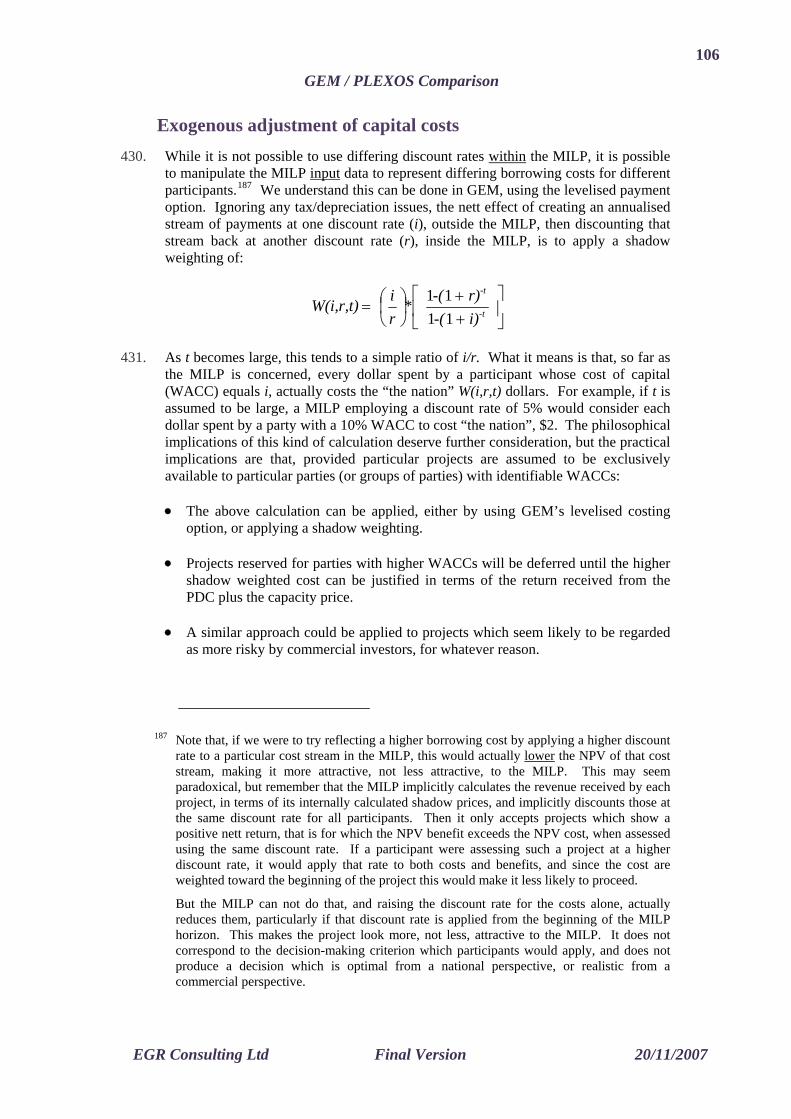
106
GEM / PLEXOS Comparison
Exogenous adjustment of capital costs 430. While it is not possible to use differing discount rates within the MILP, it is possible
to manipulate the MILP input data to represent differing borrowing costs for different participants.187 We understand this can be done in GEM, using the levelised payment option. Ignoring any tax/depreciation issues, the nett effect of creating an annualised stream of payments at one discount rate (i), outside the MILP, then discounting that stream back at another discount rate (r), inside the MILP, is to apply a shadow weighting of:
⎥⎦
⎤⎢⎣
⎡++
⎟⎠⎞
⎜⎝⎛=
i)-(r)-( *
ri W(i,r,t) -t
-t
1111
431. As t becomes large, this tends to a simple ratio of i/r. What it means is that, so far as the MILP is concerned, every dollar spent by a participant whose cost of capital (WACC) equals i, actually costs the “the nation” W(i,r,t) dollars. For example, if t is assumed to be large, a MILP employing a discount rate of 5% would consider each dollar spent by a party with a 10% WACC to cost “the nation”, $2. The philosophical implications of this kind of calculation deserve further consideration, but the practical implications are that, provided particular projects are assumed to be exclusively available to particular parties (or groups of parties) with identifiable WACCs:
• The above calculation can be applied, either by using GEM’s levelised costing option, or applying a shadow weighting.
• Projects reserved for parties with higher WACCs will be deferred until the higher shadow weighted cost can be justified in terms of the return received from the PDC plus the capacity price.
• A similar approach could be applied to projects which seem likely to be regarded as more risky by commercial investors, for whatever reason.
187 Note that, if we were to try reflecting a higher borrowing cost by applying a higher discount
rate to a particular cost stream in the MILP, this would actually lower the NPV of that cost stream, making it more attractive, not less attractive, to the MILP. This may seem paradoxical, but remember that the MILP implicitly calculates the revenue received by each project, in terms of its internally calculated shadow prices, and implicitly discounts those at the same discount rate for all participants. Then it only accepts projects which show a positive nett return, that is for which the NPV benefit exceeds the NPV cost, when assessed using the same discount rate. If a participant were assessing such a project at a higher discount rate, it would apply that rate to both costs and benefits, and since the cost are weighted toward the beginning of the project this would make it less likely to proceed.
But the MILP can not do that, and raising the discount rate for the costs alone, actually reduces them, particularly if that discount rate is applied from the beginning of the MILP horizon. This makes the project look more, not less, attractive to the MILP. It does not correspond to the decision-making criterion which participants would apply, and does not produce a decision which is optimal from a national perspective, or realistic from a commercial perspective.
EGR Consulting Ltd Final Version 20/11/2007
107
GEM / PLEXOS Comparison
• The implication will be to “bias” the solution towards development of projects with lower risks, and/or by participants with lower borrowing costs.
• If transmission and generation are jointly optimised, and Transpower is believed to have a lower borrowing rate than generators, the solution will also tend to favour transmission investment over generation investment.
432. The implications are a bit more extreme if particular projects are not assumed to be exclusively available to particular parties, and those parties have different WACCs. In that case, the party with the lowest WACC might logically be expected to buy out development options secured by other parties, so that it builds all new projects, and its modelled market share will grow progressively over the horizon.188 A MILP optimisation will naturally produce such a solution, if offered the choice of project alternatives differentiated by WACC. Fortunately, ownership does not really matter in a pure MILP environment, because it makes perfectly competitive assumptions. It will be an issue if generator gaming is to be modelled, though, and a similar consideration arises with respect to the HVDC cost recovery charges, as discussed below.
433. As stated above, we do not believe it would be appropriate to assume different borrowing costs for different generator investors, even if this can be achieved by exogenous manipulation of the data. But it may well be appropriate to use this mechanism to model the application of different borrowing costs to different project types.
6.3. Transmission Investment and Cost Recovery
434. As noted in a previous submission, there is an inherent circularity involved in SOO scenario formation.189 Ultimately, generation and transmission investment must be seen as co-dependent, and inextricably inter-related. Thus one cannot form realistic generation scenarios without also forming matching transmission scenarios, and vice versa. In this context, it seems best to view the SOO scenarios as effectively defining a starting point for an iterative process. Accordingly, it may be argued that the assumptions made about transmission investment in the SOO scenarios are not actually too critical. But that also means that the generation scenarios, per se, are not too critical either, because they will have to be re-optimised as transmission plans are refined. Hence our focus on the structural assumptions implicit in the methodology by which these scenarios will be re-optimised.
435. The way in which transmission planning, and associated cost recovery, is modelled may have a significant bearing on projected market incentives, and hence investment,
188 In fact, it should logically be expected to buy out all existing projects, too. 189 E G Read Commentary on EC Analysis of Transpower's 400 kV Proposal under the GIT
EGR Consulting report to Mighty River Power, June 2006. See http://www.electricitycommission.govt.nz/pdfs/submissions/pdfstransmission/draft-decision/MRP3.pdf
EGR Consulting Ltd Final Version 20/11/2007
108
GEM / PLEXOS Comparison
though. For example, some transmission pricing regimes may imply that particular generation projects will be charged for particular transmission system investments. The form of the transmission pricing rule can have a significant impact in the real world. The way in which the rule is modelled can have a significant impact on model solutions, too, but does not necessarily make them more realistic if it implies incentives which are not consistent with those in the real world. This is particularly true if the transmission pricing rule itself is not consistent with national economic benefit maximisation, which is always the underlying driver in MILP modelling.
436. The critical issue, here, is whether the MILP co-optimises generation and transmission expansion, or simply optimises generation expansion for a specified transmission expansion plan.
6.3.1. Cost recovery with co-optimisation 437. It might be thought that co-optimisation was desirable, in the GIT process, if not the
SOO.190 But it should be recognised that it will be difficult, if not impossible, to model any transmission pricing rule which is not consistent with national economic benefit maximisation, and hence with MILP optimisation, in a co-optimising model. In our Preliminary Critique we suggested that, in order to be consistent with co-optimisation, the transmission pricing rule would have to:
a) Distinguish between transmission system costs which have already been committed, or will be committed irrespective of the targeted generation developments, and those which are truly contingent on those developments proceeding;
b) Distinguish between generation system projects which have already been committed, or will be committed irrespective of the transmission system development proceeding, and those which are truly contingent on the transmission developments proceeding;
c) Ensure that the cost of incremental transmission investment is wholly, and solely, recovered from incremental generation projects which actually trigger that transmission investment.
438. We did not examine what such a cost recovery rule would actually imply, though, and the situation is a little complicated:
• If the capacity expansion model was an LP, with transmission capacity expansion optimised, “cost recovery charges” would actually be implicit in the inter-island price differentials, which would be sufficient to pay for the expansion.191 This is
190 That is, co-optimising the decision under consideration in the GIT application. The
optimisation of other transmission developments, not already committed, may also be performed by these models, and should be regarded as just part of the scenario simulation, like generation investment.
191 Of course those differentials would apply to all participants, but a MILP optimisation is consistent with an implicit assumption that incumbent plant already has FTRs assigned to protect then against any change in the differential.
EGR Consulting Ltd Final Version 20/11/2007
109
GEM / PLEXOS Comparison
consistent with expansion costs being fully recovered from new generation, with FTRs assigned to return any nett rents.192 Costs are implicitly recovered in proportion to actual generation (nett of FTRs) in each hour, at the inter-island price differential for the hour.193
• If the capacity expansion model is a MILP, though, the situation is different. An integer transmission capacity expansion decision will almost certainly reduce rents to well below cost recovery levels,194 and explicit (supplementary) “cost recovery charges” are likely to be required. In the limit, such implicit charges could absorb all of the nett benefits delivered by the expansion cost. But this means they would have to be levied on all participants (not just South Island generation), in proportion to benefits received, eg by lowering prices in the North Island.
439. Thus MILP optimisation, and national cost-benefit optimisation, can ultimately only be consistent with an optimal economic “beneficiary pays” approach to transmission cost recovery.195 And even that assessment is complicated by the realisation that many of the benefits received by beneficiaries will be offset by dis-benefits to other participants (eg North Island generation, and South Island loads, if the inter-island price differential falls). Thus, in our opinion, there is actually no optimal “pricing rule”, but rather an optimal pricing/contracting regime, in which the equilibration of regional contract markets plays an important role.196
440. In our Preliminary Critique, we suggested that an optimal transmission cost recovery rule could be consistently modelled in a MILP optimisation. If transmission investment was modelled as a continuous variable, or as a series of generation-linked investment increments, we suggested the transmission costs could be directly associated with generation investment variables, so that the transmission investment costs essentially became part of the generation project investment cost. But that suggestion now needs to be reconsidered. If generation and transmission are co-optimised in the MILP, then:
• If the transmission expansion cost were to be modelled as being linear, as in the above paragraph, then there would be no need to associate cost recovery charges
192 Thus new generation would only proceed if it delivered benefits in excess of the expansion
cost. But “new generation” here may include increased generation from existing plant. 193 In reality, generators may be able to manipulate output to avoid creating congestion rentals,
but that actually makes no difference if FTRs are assigned, as assumed here. 194 “Lumpy” investment, per se, will just cause rents to fluctuate around the cost recovery level.
But there is a systemic cost recovery problem here, of the order of 70-90%, arising out of strong scale economies. See E.G. Read: "Pricing and Operation of Transmission Services: Long Run Aspects". In A Turner (ed.) Principles for Pricing Electricity Transmission, Trans Power, 1989.
195 This is actually consistent with a “discriminating monopolist” approach to cost recovery, and should NOT be confused with the kind of flow-tracing heuristic approaches which have been confusingly labelled as “beneficiary pays” in some public discussions.
196 See discussion in E G Read Locational Transmission Pricing: A Formulaic Approach EGR Consulting report to Mighty River Power, February 2007.
EGR Consulting Ltd Final Version 20/11/2007

110
GEM / PLEXOS Comparison
with particular developments. In fact we have just argued that there would be no justification for explicit transmission cost recovery charges at all. If such charges were to be modelled, in the MILP framework, we should also model the assignment of FTRs which effectively give South Island generators access to North Island prices. But, if we model them as being connected in the South Island, and thus receiving South Island prices, we should not model them as also paying HVDC cost recovery charges.
• In reality, though, a realistic co-optimisation would have to associate transmission expansion costs with integer variables. In that case, there would be a justification for explicit transmission cost recovery charges, in reality, but still no reason, or mechanism, to assign them to particular projects in a MILP formulation. As explained above, the MILP optimisation already implicitly mimics the effect of an optimal economic “beneficiary pays” approach to transmission cost recovery. There is no cost to be accounted for apart from the transmission cost already associated with the investment variable, and no simple formula to assign that cost to participants.197 Generation projects will proceed, in the MILP, if and only if they collectively deliver sufficient national benefit to at least cover any associated (modelled) transmission expansion cost. And transmission projects will proceed, in the MILP, if and only if they deliver sufficient national benefit by allowing generation projects to deliver power to meet demand.
441. As noted in our Preliminary Critique, if transmission investment is optimised in the model, the transmission cost will have to be assigned to the transmission investment variable(s), and that means the cost will be double-counted if also assigned to South Island generation investment variables. Clearly, this would imply mis-computation of the model objective function, and a sub-optimal investment projection, from a national economic benefit perspective. Whether or not transmission and generation investment are directly linked in the model, this sub-optimality would apply to both generation and transmission investment plans and the latter, at least, will be inconsistent with the optimisation of transmission investment required under the GIT.
442. Thus it would be inappropriate to assign full cost recovery charges to participants, as well as charging the full expansion cost, in a co-optimised model. The issue is, though, whether it is possible, or desirable, to assign supplementary charges, so as to align the modelled incentives better with real-world incentives, as determined by actual cost recovery rules. We assume this would be done by adjusting the capital cost of particular South Island generation projects.
443. The critical issue is, of course, whether the modelled generation investment (and only that investment) would actually be commercially sustainable. Before considering any detailed assignment of cost recovery charges to generators, though, there are three conflicting factors to consider, at an aggregate level:198
..........................................................................................continued overleaf
197 And, if there was, it would not assign all costs to South Island generation. 198 Two other issues may also be considered relevant:
- Due to scale economies, the transmission investment itself will generally not be “commercially sustainable” at the modelled prices. But there will still be a positive rental stream modelled in the MILP, and this will be implicitly netted off the assignment of the costs to participants. In this respect the MILP is actually consistent with a rule which
EGR Consulting Ltd Final Version 20/11/2007
111
GEM / PLEXOS Comparison
• If some element of the cost recovery charge is shared with existing generation, the necessary adjustment should actually be negative. Since the optimisation already implicitly defers entry until it can collectively cover the full expansion cost, the effect of cross-subsidisation will be to encourage faster entry, and this should be reflected by reducing, not increasing, effective entry costs. This will also increase the apparent value of link expansion, and so bring that forward, which is sub-optimal, but appropriate given the extra South Island generation investment which would be induced by this form of cross-subsidisation.
• On the other hand, if some element of the cost recovery charge for existing HVDC assets is levied on new generation, the effects would be the opposite.
• If, as seems likely, some element of the cost recovery charge should optimally be assigned to parties other than South Island generation, the cost recovery charge implicitly assigned to South Island generation in the MILP will be less than that assigned to South Island generation in reality. Thus, ignoring the conflicting effects just noted, the MILP will tend to recommend more investment in South Island generation than may occur in practice.
444. The nett effect of these conflicting effects is unclear, and will obviously depend on several parameters. An approximate balance could be determined between the first two effects on the basis of input data, although that balance will change as the proportion of “new” generation” increases, over time. The third factor can only be assessed from model results, and perhaps accounted for iteratively. But even if all this analysis can be performed, at an aggregate level, it is not obvious how to determine adjustments to be applied at an individual participant level. As discussed above, there is no explicit, or easily calculated, assignment of costs to participants in a MILP optimisation. So it is not clear how we can determine optimal adjustments to align that implicit, and unknown, endogenous cost assignment with any particular cost recovery rule. Partly for that reason, we turn to consider the situation which arises when transmission and generation are not co-optimised.
6.3.2. Cost recovery without co-optimisation 445. The alternative to co-optimisation is for each MILP optimisation to assume that
HVDC investment (in this case) will proceed at a fixed date. This means that the transmission investment is not optimised in the model, so that the analyst (or perhaps some exogenous heuristic procedure) becomes responsible for assessing the nett
assigns all costs to participants, on the assumption that any rentals are then rebated to those participants.
- If generation investment is also represented by an integer variable there is no guarantee that it will be sustainable at the modelled prices, but this is true in any case, irrespective of transmission expansion. For South Island generation, the impact of integer optimisation of transmission expansion will be to raise South Island prices above long run equilibrium levels before the expansion occurs, possibly bringing forward some developments in that period, and then to depress South Island prices below long run equilibrium level after the expansion occurs, possibly delaying some developments in that period. But this is not unrealistic.
EGR Consulting Ltd Final Version 20/11/2007
112
GEM / PLEXOS Comparison
benefits of any transmission development by comparing model runs with differing timings, etc.
446. This approach avoids double-counting HVDC costs within each MILP optimisation. In fact there is no HVDC investment variable in the model to which generation investment decisions could be linked, and so no consideration of HVDC cost at all in the optimisation of generation investment. Thus, on its own, it will actually model generation investment as proceeding as if there was no HVDC transmission cost recovery charge at all.
447. If the HVDC investment is expected to occur irrespective of any new investment in South Island generation, there is no rationale, in terms of national economic benefit optimisation as modelled by MILP, for recovering its cost from those investments. Thus this modelled result would actually be optimal, from a national cost benefit perspective, if the HVDC investment really is not linked to new investment in South Island generation. If there is such a linkage, the analyst would model this, outside the MILP optimisation. In principle, the analyst could go through an analytical process analogous to MILP co-optimisation, and determine the co-optimised optimum. Since the solution is the same, the observations made above about cost recovery charges would still apply, even though the algorithm used to find that solution was different. In other words, a feasible and optimal allocation of cost recovery charges would exist, and could be found once the optimum had been determined, but would not conform to any likely pre-determined rule.
448. If that result was desired, though, co-optimisation should be employed. The relevant question, here, is whether the analyst could go through an analytical process to determine the optimal transmission expansion programme, given that the market will respond with sub-optimal investment, because the transmission cost recovery rules are sub-optimal. In order to do this, it seems the analyst would need to:
• Decide from which year any HVDC upgrade options, and related cost recovery charges, will be assumed to apply, for this particular MILP optimisation;
• Determine the nett effective cost recovery charges that would apply to each potential South Island generation project, before and after (each) HVDC upgrade;
• Assign the relevant annual charges to the project “existence” variable, so that they get assigned to the project for each year in which it actually exists;199
• Perform a MILP optimisation in which those cost recovery charges are assigned, as discussed above;
199 This may not be the best way to do this, but there is no single transmission cost recovery
charge which can be attached to a generation investment, irrespective of when it occurs. An alternative is to calculate the cumulative NPV charges from each possible construction date, and assign them to the project investment variable for that date. Or, if the cost recovery charge formula is based on something else, like generation, it could possibly be assigned to that variable.
EGR Consulting Ltd Final Version 20/11/2007

113
GEM / PLEXOS Comparison • Remove the cost recovery charges from the optimisation results, since they are
not true national costs, only transfers; and
• Subtract the actual NPV transmission investment costs from the optimisation results to produce a nett national benefit which can be compared with that calculated, in the same way, for alternative upgrades/timings.
449. The end result, that is the transmission expansion plan that yields the highest nett national benefit based on this kind of comparison, will be sub-optimal, from a national economic benefit perspective, but it will be the optimal transmission plan given a realistic market response to the modelled transmission cost recovery rule. The remaining issue is, then, how to determine the nett effective cost recovery charges that would apply to each potential South Island generation project, before and after (each) HVDC upgrade.
450. This is a little tricky, because the currently proposed transmission pricing rule does not distinguish between old and new costs, or between old and new generation capacity. In fact we understand that current policy is to recover all HVDC costs, both old and new, from all South Island generation, in proportion to some measure of total generation capacity, both old and new. So cost recovery charges are not really levied on individual projects, each owned by a distinct participant, as implicitly assumed in a MILP model. Nor are they all levied on a whole group of projects all owned by a single participant. In reality, the owners of existing projects, and likely proponents of new projects, each own project portfolios, of varying sizes, and their incentives will be determined by the aggregate impact of the charging policy on that portfolio.
451. This makes the situation more complex because the cost recovery rule means that any new generation investment, by any party, implies a re-allocation of both existing and new cost recovery charges between all parties. Parties that do not expand generation capacity will face increased HVDC charges if expansion by other parties triggers expansion. In fact the allocation of these costs will depend far more on the relative size of incumbents than on the size of any new investment. This also means that different parties will face different investment incentives, which cannot all be optimal.
452. In our Preliminary Critique we argued that this means that the impact of such a rule cannot be modelled in a MILP formulation, if for no other reason than that the implied cost allocation is non-linear. And we discussed several very different cases, depending on both the form of the cost recovery charges, and the logic assumed to be driving transmission expansion. That discussion is complex because it is concerned with overall optimality, in national cost benefit terms, as well as with realistic modelling of market behaviour. But much of it really only applies to a MILP which co-optimises generation and transmission.200
453. The situation is simplified, though, if the transmission optimisation is taken out of the MILP, and performed by the analyst, as proposed here. In that case, the goal of overall co-optimised optimality, in national cost benefit terms, can be abandoned, and
200 And it is almost certainly inaccurate, in some respects, because it assumes that simple
linkages can and should be created in such an optimisation, and does not account for some further complexities identified in this report.
EGR Consulting Ltd Final Version 20/11/2007
114
GEM / PLEXOS Comparison
replaced by one of “second best” optimality, given the cost recovery rules. But even that goal is only to be pursued by the analyst, outside the MILP. Within each MILP, the goal is really realism, with respect to the generation investment schedule. The associated transmission cost recovery charges, which are ultimately discarded in the meta-analysis, are only important as drivers of that investment schedule.
454. Thus all we have to determine is the nett effect, on the owner of each generation portfolio, of adding a generation investment to that portfolio. As noted above, this depends critically on the current size of that portfolio.
Signals for small investors 455. For a small independent investor, this assessment is relatively simple:
• If it builds now, it would face a per MW charge equal to the ratio of the existing cost recovery requirement to the existing MW capacity of the SI generation system, as measured by the appropriate formula. This will change very little for projects of the size such a participant is likely to propose.
• If it plans to build in a future year it would face a per MW charge equal to the ratio of (existing plus new transmission cost recovery requirements) for that year, to the (existing plus planned MW capacity of the SI generation system), for that year.
456. Given the way in which cost recovery charges increase after each expansion, this implies incentives to invest more, prior to expansion, ignoring the possibility that this may trigger expansion, and less after transmission expansion, ignoring the new (physical) opportunity created.201 The dynamic pattern of this price signal is not just sub-optimal, but exactly the opposite of what it should be from a national cost benefit perspective. And there is an additional constant, and economically inappropriate, dis-incentive implied by the recovery of existing system costs from a new investor, whose actions do not increase those costs. But this is a realistic reflection of the transmission pricing methodology.202
201 The small investor will respond appropriately to the decreased inter-island differential
created by expansion, but the impact of cost recovery charges will dampen, and quite possibly reverse, this otherwise optimal response.
202 The 2007 paper by Read referred to in FN 196 above (following the work by Read[1989], as in FN 194) argues that it is simply not possible to provide appropriate economic signals using any pricing methodology which attempts to allocate costs once sunk, on the basis of any measure of participant “use” of transmission capacity, As determined by operational behaviour. Our observation here merely extends that comment by observing that the same is true if such backward-looking price mechanisms are applied on the basis of participant investment (rather than operational) behaviour, since investing in a facility is an inevitable precursor to using it. The paper argues that, with scale economies in transmission expansion optimal economic signals can only be provided by a regime which relies on forward looking contracting, not backward looking pricing. Or, they may be approximated by a regime which charges for all participants are truly fixed, say on the basis of market shares prior to expansion, for some period after expansion, irrespective of operational or investment activity in that period.
EGR Consulting Ltd Final Version 20/11/2007

115
GEM / PLEXOS Comparison
457. Analytically, the only problem is that we do not actually know what the planned MW capacity of the SI generation system will be until we solve the MILP. This means we do not know the per MW cost recovery charge.203 Thus iteration may be necessary to get an internally consistent result.
Signals for a monopoly investor 458. For a monopolist, the appropriate nett cost recovery charge to assume in a MILP
optimisation is arguably zero. This reflects a judgement that HVDC cost recovery charges of the proposed form, whether for new or existing assets, imply no dis-incentive at all to generation expansion by a monopolist, because they would face the full cost anyway.
459. Since each MILP optimisation assumes a fixed transmission investment schedule, the implicit assumption here is that the monopolist’s investment activity has no impact on transmission investment. If that is truly the case, the implied incentives for a monopolist are actually optimal from a national cost benefit perspective. From a national cost benefit perspective, and from its own, the monopolist may as well plan to use the capacity provided as best it can, irrespective of any cost recovery charges, since the costs are committed, and the charges are only transfer payments.
460. This also seems to be a realistic commercial strategy for the monopolist to adopt, once the capacity has been committed, or if the monopolist believes it can not influence the expansion decision. We consider the impact of relaxing this assumption below, but note that, while the signal implied by the cost recovery rule under these assumptions may be sub-optimal from a national cost benefit perspective, it is at least not counter-cyclical like the signal implied for small investors. If no cost recovery charge is modelled in the MILP, the monopolist will at least respond appropriately to the reduction in inter-island differentials following expansion, and this will tend to favour some degree of pro-cyclical investment. But what this regime will not do, under these assumptions, is to incentivise the monopolist to consider the reduction in national economic cost which could have been made if it had moderated its behaviour prior to expansion, in such a way as to delay the need for expansion.
Gaming by a monopoly investor 461. In reality, market power is a consideration here, though. If the monopolist thinks that
it can delay transmission investment, and hence avoid any increase in transmission cost recovery charges, it may be in its interests to delay generation investment, and/or limit output, in order to avoid triggering transmission expansion. Perhaps surprisingly, that “gaming’ response actually incentivises pro-cyclical operational and investment behaviour which, in the limit, would be optimal, from a national cost benefit perspective. Thus it appears that the optimal (gamed) response of a
203 The MW capacity of the small investor’s own portfolio may be considered irrelevant, so
long as it remains “small”.
EGR Consulting Ltd Final Version 20/11/2007
116
GEM / PLEXOS Comparison monopolist could actually be modelled by a co-optimised MILP, even though MILP optimisation allows for no explicit consideration of gaming incentives.204
462. To represent the effect of such gaming in a model which does not co-optimise, cost recovery charges assigned to the monopolist would have to increase before expansion was planned to occur, and then decrease afterwards. This is the exact opposite of the dynamic pattern of the actual cost recovery charge, but it does provide better (and potentially optimal) economic signals, from a national cost benefit perspective, and corresponds to a realistic assessment of the monopolist's incentives, once gaming is accounted for.
463. The issue is, though, whether such behaviour is realistic, even if a monopolist exists. Arguably, it could be assumed for future transmission developments, which could thus be co-optimised. The monopolist's strategy would be to restrict its output, and to restrain itself with respect to announcing any development plans or prospects as being likely to occur prior to the date at which it thinks an upgrade would serve its own interests, and then to optimise its plans to utilise the planned capacity, once it is committed.
464. But the period in which any influence might be effectual is not immediately prior to expansion, but prior to the time of commitment. Thus the prospects of influencing an imminent transmission investment decision by mere behavioural change might be thought slim.205 From an analytical perspective, it might reasonably be assumed that any such “games” have already been played, with respect to the decision at hand, and are already accounted for in the data.
465. If such gaming were to be modelled, it would further increase the divergence between the incentives of the monopolist and the independent investor. If no cost recovery charges are modelled for the monopolist, its incentives to invest before or after the transmission expansion will be driven entirely by short run prices, ignoring any cost recovery charge. Modelling of gaming would give the monopolist additional incentives not to invest before expansion occurs. By way of contrast, an independent investor has additional dis-incentives for investment before expansion,206 but even stronger dis-incentives afterwards.207 Thus it might be thought best to simply ignore any gaming incentives, and model a monopolist as paying no cost recovery charges in
204 This should not really be a surprise, because the MILP effectively models vertical
integration, in which the externalities implied by the cost recovery charge rules are internalised, which is appropriate for a monopolist.
205 A more credible mechanism to signal firm intentions of this type would be by forward contracting in energy and/or FTR markets, but that is probably not an effective signalling mechanism in the current New Zealand context.
206 To avoid cost recovery charges for the existing transmission system, the costs of which are actually sunk, from a national cost benefit perspective. If we ignore gaming, the independent investor actually has greater dis-incentives, even in this period, than the monopolist, but the balance is not clear once gaming is accounted for.
207 To avoid cost recovery charges for the existing and new transmission systems, the costs of which will then be sunk, from a national cost benefit perspective.
EGR Consulting Ltd Final Version 20/11/2007

117
GEM / PLEXOS Comparison
the MILP, rather than introduce the counter-cyclical pseudo-charges which would be necessary to model optimal behaviour.208
Cost recovery charges for real investors 466. Real cases will involve several parties spread across the spectrum from small
independent entrants, to prominent, if not dominant, incumbents. Given the way in which this aggregate charge is re-distributed by incremental generation investment, and the degree to which each may consider its behaviour can influence HVDC investment decisions, the nett effect on proponents could be either pro- or anti-cyclical. Either way, the pricing rule implies that the incentives applicable to particular projects will vary non-linearly, depending on who proposes them.
467. Accurate modelling would require a detailed, and somewhat circular, analysis to determine likely proponents, and hence likely incentives. It will be evident that the largest incumbent always faces the least dis-incentive, from cost recovery charges, to further development of any kind. In fact MMA have calculated that the effective cost recovery charge varies linearly, from 100% of the combined cost recovery charge for existing and new assets for a small investor, down to 0% for a monopolist. This aligns with the discussion above, if gaming can be ignored.
468. Other things being equal, the logical conclusion of this analysis could reasonably be that if any potential entrant secures an option for a development, they would always be best to sell their interest in that development to the largest incumbent.209 If so, we could assume that the largest incumbent would develop all future projects, and gradually increase its market share over time.210 This may actually seem desirable, from this perspective, in that it implies a gradual reduction in inappropriate dis-incentives for South Island generation investment. But it is obviously less desirable from other perspectives. Nor is it inevitable, because other off-setting factors do apply.
469. In reality, it seems likely that participants will continue investing in patterns corresponding to their existing activities. It seems unlikely that further development of major river chains will be pursued by anyone other than the incumbents, and those projects can safely be assigned accordingly. And it seems reasonable to assume that projects which have been identified with particular proponents in the existing database will actually be pursued by those proponents, or not at all. If, in future, those projects were to be taken over by larger incumbents, our current assessment of
208 It should be recognised, though, that this amounts to saying that even a monopolist South
Island generator could not influence the timing of HVDC investment. This should give pause for thought with respect to the optimality of both the HVDC cost recovery rule and the GIT process.
209 This is analogous to the effect of one party having a lower borrowing cost than another, as discussed in Section 6.2. The effects will reinforce each other, if larger parties have lower borrowing costs than smaller ones.
210 The same logic might be thought to imply incentives to take over existing plant too, leading to an eventual monopoly. Our preliminary analysis suggests that this is not the case, but we have not confirmed that conclusion.
EGR Consulting Ltd Final Version 20/11/2007
118
GEM / PLEXOS Comparison
e incumbents.
could be applied even to projects with identified proponents in the current database.
e assignments. Iteration may be necessary to get an internally consistent result.
he transmission expansion plan is specified exogenously in each MILP optimisation.
should follow the outline proposed in Paragraph 448 above, augmented as follows:
their effective profitability might turn out to be a too low, but there must be significant doubt about these projections anyway.
470. It also seems reasonable to assume that there would be resistance, at some level, to takeovers which increased the market share of larger incumbents. It might be possible to assign notional ownership of generic projects in such a way as to approximately preserve current market shares.211 Or it has been suggested that market share constraints could be imposed. Although this may be considered artificial, it might be argued to represent a realistic reflection of likely policy. If so, the above logic suggests that the constraints limiting growth of the largest players will probably turn out to be binding. Thus they would have a positive shadow price, which would imply a uniform cost penalty to all of potential developments by larg
471. If ownership is pre-assigned, this would have the effect of delaying those projects long enough to just keep pace with the aggregate growth rate of other participants. With such constraints in place, though, there is no need to pre-assign ownership of all projects. Alternatives can be created in the data base which differ only with respect to ownership, and hence with the cost recovery charges assigned. The MILP will no longer automatically choose the cheapest of these options; that is the one which would be owned by the largest incumbent. Instead, the shadow price on the market share constraint could deter entry of that option, under that ownership, in favour of development of the same physical option, under different ownership. This does not seem an unreasonable representation of the way in which market mechanisms might actually work, under an implicit market share constraint, and
472. Analytically, the problem remains, though, that until we solve the MILP, we do not actually know the planned MW capacity of the South Island generation system, or of any generation portfolio, for any future year. Thus we do not know future market shares, or cost recovery charg
212
6.3.3. Implementation using GEM/PLEXOS 473. Implementation of these ideas obviously depends critically on whether the MILP
optimisation co-optimises transmission expansion, or at least the transmission project under consideration, with generation expansion. If it does, we have argued that consistent implementation of a sub-optimal transmission cost recovery rule may be very difficult. Partly for that reason, we have focussed mainly on the case where t
474. If that approach is accepted, implementation
211 The feasibility of this depends on the market share trends implied by the current dataset,
which we have not examined. But we note that projects assigned to larger incumbents will still tend to get built earlier, thus increasing market share more quickly.
212 Although this could be avoided if we can assume that current market shares are maintained throughout the optimisation horizon.
EGR Consulting Ltd Final Version 20/11/2007
119
GEM / PLEXOS Comparison
a) Introduce market share constraints into the MILP, if desired;
b) Decide from which year any HVDC upgrade options, and related cost recovery charges, will be assumed to apply, for this particular MILP optimisation;
c) Determine the likely ownership of each potential South Island generation project, and/or create alternatives under different ownership if market share constraints have been imposed;
d) Determine the nett effective cost recovery charges that would apply to each potential project, before and after (each) HVDC upgrade, given its assumed ownership, and estimated future market shares, with or without accounting for potential gaming by larger participants as discussed in Paragraph 461 above;
e) Assign the relevant annual charges to the project “existence” variables, so that they get assigned to the project for each year in which it actually exists;
f) Perform a MILP optimisation in which those cost recovery charges assigned;
g) Re-consider the market shares implied by the solution, adjusting the charges calculated in Step (d), and re-solving if necessary;213
h) Remove the cost recovery charges from the optimisation results, since they are not true national costs, only transfers; and
i) Subtract the actual NPV transmission investment costs from the optimisation results to produce a nett national benefit which can be compared with that calculated, in the same way, for alternative upgrades/timings.
6.4. Market Implications of Capacity Requirement Modelling
475. Our Preliminary Critique stressed the point that, while a MILP optimisation may simulate a perfectly competitive market, it will only guarantee revenue adequacy for new generation investment in a perfectly competitive market that is designed to correspond exactly to the MILP mathematical structure. If that structure only requires that energy requirements be met in each period, then the energy prices it calculates should be able to support the entry it projects, in a period by period energy only market.214 But if the MILP model also includes capacity constraints, and if those constraints prove to be binding,215 then the entry projected by the MILP will only be
213 Given the number of times this optimisation would be repeated for different timings,
scenarios etc, it should be possible to estimate market shares fairly accurately, before performing a MILP optimisation, thus hopefully eliminating any need to re-solve for this reason alone.
214 But note comments in Section 4.3.7 with respect to the procing implications of integer investment variables.
215 This will be assumed throughout our discussion.
EGR Consulting Ltd Final Version 20/11/2007

120
GEM / PLEXOS Comparison
supported in a market which also includes capacity payments, reflecting the shadow prices on the MILP capacity constraints.216
476. Since the New Zealand electricity market does not include capacity payments, this calls into question the credibility of market projections produced by a MILP optimisation in which capacity constraints are included. Specifically, we asked whether projections made on this basis are actually realistic, in the sense that they represent the implications of a policy to which the Commission has made a commitment firm enough that it can be assumed as a basis for both generation and transmission planning.
477. As we understand it, Commission staff have responded that the Commission is committed to ensuring that security requirements are met, and to introducing any mechanisms which are found to be necessary to achieve that goal. This is obviously a reasonable position for the Commission to take, and provides justification for including some form of capacity constraint in the model. But the nature of the constraints, and the way in which they are implemented, should really depend on the nature of both the criteria and the mechanisms by which they are intended to be met.
478. Section 5.3 discusses the three kinds of “capacity constraint” that might reasonably be expected in model of the New Zealand electricity sector, namely spinning reserve, contingency coverage, and dry year energy capability. That section also discusses the formulation of such constraints, and their implications from a national cost benefit perspective.
479. Spinning reserve is really a market issue, given the New Zealand market design, and our simplistic discussions based on the “energy-only” PDC should really be generalised to include both energy and spinning reserve prices. This will add a profit component which helps to ensure revenue adequacy of sufficient new plant to ensure that both energy and spinning reserve requirements are met. Beyond that, though, the implications of modelling this type of constraint seem much the same in a market environment as they would be in a centrally planned environment.
480. Just ignoring this requirement would obviously lead to modelled market investment being too low. GEM does not ignore spinning reserve, but includes it in a generic capacity constraint, thus increasing the apparent reliance on capacity constraints, and hence reducing the credibility of the results, in a market which does not have any capacity payment mechanism, other than the spinning reserve price. In Section 3.3 we have argued that this approach will also lead to energy prices being understated, because it does not really represent the true cost of meeting spinning reserve requirements.
481. Planning capacity investment on the basis of expected flows would lead to energy prices, and market investment, being understated, too. But, as discussed in Section 5.3, GEM does not do this either. Instead it runs a capacity investment optimisation assuming a very dry year. We have argued that this will not produce a balanced capacity investment plan, from a national cost benefit perspective. But it is clearly
216 As discussed in Section 4.3.7, an implicit capacity price component may arise in a MILP
model anyway, but we believe this will be fairly minor, unless capacity constraints are also imposed.
EGR Consulting Ltd Final Version 20/11/2007
121
GEM / PLEXOS Comparison not a realistic projection of market investment, either. The optimisation will project investment in too much base/mid-range plant, on the assumption that it would actually be used to meet the residual dry-year LDC, with 100% probability. This is not appropriate as a simulation of likely investment in an energy-only market, and nor is it appropriate as a simulation of the effects of any likely capacity mechanism.
482. It may be argued that these effects can be counteracted by adding a capacity constraint which encourages investment in peaking capacity. This will have a balancing effect, and may even produce an optimal balance. But the situation does not seem very satisfactory, because:
• It means that the modelling system is not attempting to produce, at any level, a realistic projection of “market” investment; and this means that
• The mix of investments projected to occur will not match what the market will actually produce without augmentation, and nor will it match what the overall regime will produce if market investment is balanced by investment in “capacity only” projects;
• There is no way to assess the degree of reliance being placed on capacity constraints, and hence perhaps on hypothetical market mechanisms intended to support investment in capacity to meet non-market security requirements; and consequently
• There is no way to make a judgement about the plausibility of the market projections, inasmuch as they may rely on these hypothetical mechanisms, and funding sources, to maintain revenue adequacy.
483. In our view, the best way to model a market investment mix that is realistic, at least with respect to hydrological variations, is to model operation of the system under a representative set of probability weighted inflow sequences in the capacity planning module. This is discussed, along with some alternative approximations, in Section 3.4.4.
484. Once a balanced capacity expansion optimisation has been performed, with factors such as spinning reserve, unit breakdowns and hydro variation modelled, it would be possible to determine what impact explicit capacity constraints, whether related to peak or dry year energy capability, might actually be having on the solution. We think it unlikely, though, that optimal market investment simulated in this way will (always) meet capacity requirements consistent with current policy settings for supply security. Thus these solutions most likely do imply some degree of reliance implicitly being placed on hypothetical capacity market mechanisms. And this creates a “credibility gap” which we believe will be an important issue for participants.
485. This is partly because there will always be factors, including low probability contingency events, which will not be modelled in the MILP optimisation, and which might collectively imply a “need” for greater capacity margins. Thus, while recognising the negative implications of increasing computation times, we consider it important that efforts be made to model those factors, where possible, so as to reduce
EGR Consulting Ltd Final Version 20/11/2007
122
GEM / PLEXOS Comparison
any credibility gap to a minimum. Even if all such factors were modelled, though, we still think it likely that a MILP optimisation based on national cost-benefit maximisation will not meet capacity requirements consistent with current policy settings for supply security at all times, under all scenarios.217
486. Thus it seems likely that a supplementary capacity mechanism will have to be introduced, in the model, if not in practice. As discussed in our Preliminary Critique, there are three broad choices.
487. First, if supplementary “capacity investment” is allowed to compete, operationally, with ordinary investment, it may be regarded as a substitute for investment which might otherwise have been justified by the marginal value of reducing shortages which will no longer be modelled as occurring. In other words, all other capacity will effectively be credited with the savings from reducing supplementary capacity investment requirements, but not also credited with savings due to reducing shortages which were costed at a level above the assumed marginal operating cost of that supplementary capacity.
488. This corresponds to an assumption that there will be a capacity ticket market, or some similar capacity pricing mechanism, with no ad hoc intervention to build special plant dedicated to only meeting capacity requirements. This option can be modelled by introducing capacity constraints into the MILP, perhaps utilising the ALDC approach discussed in Section 5.3. That formulation would not make any hard distinction between plant built to meet the capacity requirement and plant met to cover LDC requirements. Nor would it impose special restrictions on the utilisation factors of plant primarily built to meet the capacity constraint also being used to meet LDC requirements. But it would probably apply different capacity factors defining the extent to which all plant could be assumed to meet the capacity requirement.
489. If MILP results produced under this assumption are analysed, we expect that it will be found that the projected generation investment is not commercially sustainable, on the basis of the market PDC determined by the MILP, but only once capacity payments are accounted for.
490. Second, if supplementary “capacity investment” is not allowed to compete, operationally, with ordinary investment, it is not a substitute for investment which might otherwise be justified by the marginal value of reducing shortages, which will still be modelled as occurring. This can be modelled by introducing capacity constraints into the MILP, and allowing investment in plant specially dedicated to
217 And we also think it likely that, even if the MILP solutions do meet policy requirements, the
real market might not did produce such solutions because of aversion to risk, including risk of government intervention, for example. Thus it is possible that the “market simulation” itself may be considered to imply unrealistic capacity investment, even before any additional capacity constraints are added. In reality, this may imply the need for a supplementary capacity mechanism. But the modelling results would not indicate the need for a supplementary mechanism, and nor would, it make any sense to model one in conjunction with model results indicating that there is no need for it.
EGR Consulting Ltd Final Version 20/11/2007
123
GEM / PLEXOS Comparison
meeting this constraint, while setting a maximum utilisation factor of zero on their contribution to meeting loads in the LDC.218
491. This formulation is consistent with the assumption that some plant will be paid solely for their standby peaking capacity, while all other capacity will effectively be credited with the savings from reducing supplementary capacity investment requirements, but also paid in the energy market. This means that they will be credited with savings due to reducing shortages which are costed at a level above the marginal operating cost of that supplementary capacity. We have suggested that this seems like a rather unlikely compromise between a capacity ticket market solution and the status quo. If an open capacity market exists it seems unlikely that peaking plant would be excluded from competing in energy markets, particularly when such a restriction could only reduce national economic benefits.
492. Third, under the status quo, intervention has occurred to build special plant to meet capacity requirements, and that plant has then been quarantined from normal market participation. To model such a policy, it would seem necessary to first perform an optimisation without any additional capacity constraints, but modelling the various factors which would cause the market to invest in such capacity as above, and then to add any supplementary investment deemed necessary to meet capacity requirements to the proposed plan, subsequent to the optimisation. This approach was taken in the GEM model used to produce SOO projections.219
493. The two-phase approach means that the optimisation model would see no reason for the economics of investing in “normal” plant to be boosted by the assumption of a capacity credit. So it would project less building of “normal” plant, available to meet the projected LDC requirements, spinning reserve etc, and presumably project a corresponding need for more supplementary plant to meet capacity requirements. This approach was taken in preparing the SOO scenarios, except that, since the first capacity optimisation was based solely on a dry year simulation, it was not really a realistic projection of likely market behaviour. This would have reduced the apparent need for “supplementary” plant, perhaps substantially.
494. This two-phase approach would obviously increase national economic costs relative to either of the fully co-optimised approaches described above. But it may be regarded as a more realistic projection if such a policy is actually to be maintained.
218 This approach could also be implemented using the ALDC concept. Plant with zero
utilisation factors will only seem more attractive than plant which is modelled as available for actual use if it is cheaper to build. But this is not implausible given the wide range of options available in building such low utilisation plant, and the possibility of special contracts which would reduce investor risk, and hence required rates of return.
219 The GEM model used to produce SOO projections included a special restriction so as to ensure that incremental capacity requirements were only met by incremental generation capacity investments. This restriction may not have actually had any impact, because load growth and retirement of existing generation would have increased the need for new generation, anyway. In any case, it has been dropped from GEM, and is not implemented in PLEXOS, so it is no longer relevant.
EGR Consulting Ltd Final Version 20/11/2007
124
GEM / PLEXOS Comparison
At least the generation investment which the optimisation model does project as being economic could then be supported by its internally calculated PDC.220
495. A similar two-phase approach could be taken if the future policy were to be that plant built under special arrangements was also allowed to compete with other plant in the market.221 The claim of realism would be more dubious in that case, though. Arguably, participants would start to anticipate the likelihood of investment under that policy, and hold off building any capacity to fulfil a backup capacity role until offered a backup contract, or given access to whatever other mechanism might be introduced to support such investment.
496. In principle, the same logic should really extend all the way down the merit order, with proponents of even base-load plant holding out to receive recognition for the fact that such plant also provides capacity in peaks and dry years. In the end, if one assumes that the Commission itself acts rationally to minimise capacity investment costs by conducting competitive tenders, or whatever, the end result is not clearly different from the first approach described above.
497. One could perform a more limited second optimisation, perhaps covering only limited plant types, in which the plant being introduced under the security regime was allowed to compete with plant whose entry had already been recommended by the primary market-simulating MILP optimisation. If so, it would seem unreasonable to fix the variables defining market-driven investment, though, because participants who expected such competition from security capacity plant could well decide not to invest. Thus the end result would again seem to be largely equivalent to that of the first approach described. The only real difference would seem to be that only certain types of plant might be eligible for whatever assistance might be available from the security capacity mechanism. This could be modelled by reducing the effective cost and/or discount rate for such plant in the primary optimisation, and eliminating any need for a secondary optimisation. But restricting plant types could only increase national costs.
498. In all of the above discussions any implicit capacity payments would be proportional to the capacity factors assumed with respect to meeting the capacity requirement. So the economics of entry by each plant type, in the model, will be boosted to a different degree, in proportion to its assumed capacity contribution factor. In market terms, this is equivalent to assuming that plant of each type would be allowed to sell capacity tickets for a proportion of its capacity determined by this capacity contribution factor.
499. Whether or not this is a realistic projection of future market conditions, it will be evident that these capacity contribution factors play an important role in determining the generation mix projected by the model. Thus the tuning of these factors to provide a realistic representation of each plant type’s contribution to the specific
220 Ignoring the more moderate capacity payments implicit created by integerisation. 221 Intermediate options could also be modelled, in which the supplementary plant installed to
meet capacity requirements might be reserved to contribute only when the marginal cost of load reduction has reached some critical level, above the actual marginal operating cost of the plant. This could be modelled by artificially setting the assumed marginal operating cost of the plant to that critical intervention level, in the MILP.
EGR Consulting Ltd Final Version 20/11/2007
125
GEM / PLEXOS Comparison
capacity requirement which the Commission intends to model is another area requiring more detailed documentation, and examination.
6.5. The Impact of Generator Gaming 500. Finally, we come to what is arguably the biggest difference between a centralised
least-cost planning environment and a market. In a market, participants are free to set their own offer prices, and these may differ from their underlying marginal costs. There is a very substantial academic literature devoted to analysing the implications of this observation, particularly in situations where some participants may be able to exploit “market power”, and engage in “gaming” practices typically designed to force market prices up. Various models have been developed to analyse these effects, but they are much more difficult to optimise, and virtually impossible in a MILP context. Thus MILP is not really an ideal technique for preparing market projections where gaming is considered to be a significant issue.
501. At best, the assumed marginal costs can be adjusted so as to reflect historical, or projected, participant offers. And these adjustments may be calibrated to match offers implied by simpler models, within which hypothetical gaming strategies may be optimised.222 We understand that some such sensitivities may be contemplated in this case, using the Cournot gaming module available within the PLEXOS suite. It is debatable, though, how much impact such gaming really has on long term investment patterns, which are the key issue here.
502. The IAEE paper by Read et al (2007)223 argues that entry economics, at least at the national level, will be driven by technology costs, irrespective of short run gaming behaviour. On average, it is argued, the market PDC must eventually rise to a level at which entry becomes economic, and can rise no higher. According to that analysis, gaming will only occur as a short run phenomenon, where the market is out of equilibrium with respect to entry in some particular regions or periods.
503. If so, gaming can ultimately only affect the pattern of prices, and not their overall level, except inasmuch as it may impact on the risk faced by potential entrants, and hence the price level at which they are prepared to enter. Others have argued that gaming is much more important, and indeed vital as a mechanism to raise the market PDC to the levels necessary to sustain sufficient entry to maintain what are deemed to be acceptable capacity levels.
504. These two viewpoints are not necessarily incompatible. The pure theory of energy-only markets rests on the assumption that participants will face absolutely no possibility of a restriction on their ability to raise prices to levels which ration demand to match available supply during any shortfall situation, and no possibility of competition from subsidised entry of plant intended to meet capacity requirements or limit price rises.224 Conversely, that same theory implies that market-driven
222 Using “Cournot” or “Supply Function Equilibrium” techniques, for example. 223 See FN 183. 224 That theory also requires that investors be risk neutral, which seems unlikely, particularly
with respect to seldom used dry year backup plant.
EGR Consulting Ltd Final Version 20/11/2007
126
GEM / PLEXOS Comparison
investment will fall below optimal levels if there is any possibility that such a restriction might be applied, or entry subsidised.
505. And this is clearly the case in New Zealand, where the threat of regulatory intervention surely means that participants know that market prices will never be allowed to rise to the levels which are theoretically optimal if a real crisis were to occur. And this means that a perfectly competitive market PDC will simply not be high enough, on average, to sustain optimal entry, matching the LRMC of new entrant plant.
506. There are several issues which could be discussed with respect to these analyses, and several controversies which will not be resolved here. But the first point to note is that failure to model gaming behaviour is not necessarily a major limitation with respect to the applicability of MILP models to simulate capacity expansion in a market environment. Or at least the discrepancies introduced by this failure are probably much less than those implied by some of the other factors discussed previously.225 For example, the related issue of choosing a discount rate which properly reflects the risk faced by intending entrants, including the risk from gaming, probably has a greater impact on the overall solution.
507. The second point is more important, though. We have argued that a MILP optimisation with capacity constraints actually models a market with capacity payments, not an “energy only” market as currently implemented in New Zealand. Alternatively, though, it could represent an energy-only market which is relying on the assumption that generators will have, and will be allowed to exercise, enough market power to push energy market prices up during non-crisis situations to compensate for any restriction on their ability to charge what the market might bear during real crises.
508. This is a legitimate policy option, and has been adopted in other energy-only markets such as Australia. Arguably it is the only feasible policy option in the absence of explicit measures to deal with the capacity adequacy issue. Otherwise the market simply cannot sustain an economically optimal level of investment.
509. Relying on gaming in this way could produce some sub-optimality in terms of system operation, and a PDC which involves more moderately high prices, but fewer extremely high prices, than might be calculated by an optimisation model. But it will not necessarily produce a different pattern of entry. In fact, the nett effect is really not much different from a traditional approach to capacity pricing, in which the cost
225 In 2006, CRAI applied their Cournot model to assess the “competition benefits” associated
with Transpower's GIT application for a 400KV upgrade to Auckland. While this analysis definitely did illustrate that a ‘gamed’ market equilibrium might differ significantly from the perfectly competitive equation projected by MILP, the overall conclusion, across all scenarios, was that the impact was relatively modest. It remains to be seen how large such effects may be in the case of the HVDC. See Analysis of Transpower's 400 KV Project and Alternatives CRAI report to Transpower, June 2006, available at http://www. electricitycommission.govt.nz/ submissions/substransmission/draftdecision/
EGR Consulting Ltd Final Version 20/11/2007
127
GEM / PLEXOS Comparison of meeting capacity requirements is met by a surcharge levied over all loads in all periods.226
510. When conceptualised in this way, the requirement is for policy settings which allow participants to game prices up to the point where the level of energy prices, alone, matches the aggregate level of energy and capacity prices which would arise in a market with capacity pricing. Other than a market price cap, it is unclear exactly what parameters can be controlled by the Commission so as to tune market conditions to provide incentives for what it considers to be an acceptable level of gaming, supporting what it considers to be an adequate level of capacity investment. It may well be possible though, in some approximate sense, and other markets are relying on this approach.
511. The need for participants to exercise such market power would become more acute if capacity requirements were imposed on the market so as to increase investment to higher levels than the unconstrained perfectly competitive market would willingly support.227 But it may still be possible, if capacity requirements are not much in excess of what the market would freely supply.228
512. Combining these two observations, we suggested that it should be understood that making projections on this basis may be read as implying an assumption that, so long as an energy-only market is maintained, gaming will be allowed to maintain prices at a high enough level to incentivise entry to meet the specified capacity requirements, and/or that a capacity market will be introduced if this approach proves inadequate, or unacceptable.
513. But both of these suggestions were a little off the mark, in that the SOO projections were not actually based on a single integrated optimisation of investment with capacity constraints in place, but rather on the two phase approach described in Section 6.4. Thus, if the underlying capacity optimisation had been a realistic simulation of market investment, it could be argued that, in releasing these projections the Commission was implicitly endorsing a view that the status quo policy, involving intervention to build peaking capacity when required, was sustainable.
514. But the underlying capacity optimisation was not a realistic simulation of market investment, and nor was it a simulation of any other likely capacity market policy. Thus it seems unlikely that the Commission actually intended to make any particular statement about future policy in issuing these projections. But, the realism of these projections is largely measured by the extent to which independent investors can be
226 Nor is it really any different from normal commercial practices accepted and expected in all
other real markets we are aware of. 227 The above discussion relates to allowing gaming to “correct” of market incentives to offset
the loss in value which would otherwise be implied by the effective truncation of theoretically optimal market price spikes, in an unconstrained market. But higher prices, and thus more gaming, would be required if policy setting required capacity investment greater than that for such a perfectly competitive market.
228 Note, though, that the balance of incentives applying to investment in different plant types may be quite different in a market which relies on gaming to shift the PDC up, for all participants, than in a market which makes explicit capacity payments, scaled in proportion to capacity contribution factors, as implicitly assumed in GEM.
EGR Consulting Ltd Final Version 20/11/2007

128
GEM / PLEXOS Comparison expected to behave in the manner simulated; that is in response to the policies implicit in the MILP formulation.
515. If those policies are not considered to be realistically sustainable, there is no guarantee that generation investment will actually proceed as projected. And, unless market participants actually have clear guidance as to the policy under which such investments can be made, and can safely expect to recover their costs, they will hesitate to do so, thus undermining the market, as well as the credibility of the SOO projections. If those projections are not made on the basis of a clear, consistent or comprehensive policy, they may well make a negative contribution by creating confusion, and increasing perceived risk in the industry. So, once more, we stress the importance of establishing a clear policy, and reflecting it consistently in the model formulation and assumptions for the SOO/GIT process.
EGR Consulting Ltd Final Version 20/11/2007