Game Theory Models in PLEXOS Game Theory Models of Imperfect Competition in the PLEXOS Software

Drayton Analytics Research Paper Series

Dr Michael Blake

Drayton Analytics,

Adelaide, South Australia

4 February 2003

I: Background

At the most basic level, competitive electricity markets result from the efficient trade of two

goods - energy and transmission services. Models of imperfect competition utilise game theory to

examine behavioural deviations by market participants from the competitive norm and their

impacts on efficient trade in these markets. This behaviour, however, is not independent from

market design and structure, which affect participant incentives and interactions. For example,

auction design, e.g. single- versus multi-part bids, in a centralised market may give participants

certain opportunities to exercise market power. Likewise, institutional arrangements in a bilateral

market may give arbitragers incentives to act in a non-competitive manner. Consequently, if

market design or institutional arrangements are poor then inefficiencies may be created that erode

the potential benefits from trade.

As a result, one way to categorise models of power markets is by the market mechanism:

• centralised – POOLCO Model

• decentralised – Bilateral Model

The majority of market power studies to date either explicitly or implicitly assume a centralised

auction process, administered by an Independent System Operator (ISO), through which

generators sell energy to consumers [3,7,11]. A growing number of studies typically assume a

decentralised trading process by which generators sell to consumers bilaterally through power

exchanges or arbitragers [14]. Metzler et al. [10] presents models that can represent both

POOLCO and Bilateral Models.

A second way to group these models is by the type of interaction that they assume about the

behaviour of participants (primarily, but not limited to, generators):

• Competitive – firms are price-takers and possess no market power

1

• Cournot – quantity is the strategic variable, and firms choose quantities simultaneously,

under the assumption that other firms’ quantities are fixed

• Bertrand – price is the strategic variable, and firms choose prices simultaneously, assuming

that other firms’ prices are fixed

• Supply Function Equilibrium (SFE) – entire bid functions are the strategic variables, and

firms choose their supply functions simultaneously, under the assumption that other firms’

supply functions are fixed; a market mechanism, e.g. an ISO, then determines price and sets

the quantity.

These are the basic paradigms currently relevant to this article. Other paradigms include, but are

not restricted to, Stackelberg behaviour and collusive behaviour. These paradigms are presently

outside the scope of this article.

The application of the different paradigms of participant interaction may produce equilibrium

outcomes with substantial variations in the intensity of competition. Consequently, equilibrium

outcomes may be sensitive to the particular paradigm selected. This sensitivity has created

significant discussion regarding the relevance of each paradigm to modelling competition in

electricity markets and has led to the development of a number of variants to each paradigm that

investigate different assumptions about market structure and design.

Section II first explains the two primary market mechanisms relevant to modelling electricity

markets, and Section III contains a detailed discussion of the specific models used in PLEXOS.

II: Market Mechanisms

True competition in electricity markets, in which competing generators sell directly to unaffiliated

distributors / retailers, did not emerge until the 1990s. Prior to this time, real markets did not

exist, and isolated ‘pockets’ of generation units operated as localised monopolies. With the

passage of time, the gradual growth in transmission network interconnection facilitated bilateral

contracting between local monopolies – a seller would contract with a buyer to deliver a certain

quantity of electricity at a specific time, and the buyer would factor this input into its unpriced,

centralised decision-making process. With scattered monopolies using networks more or less

exclusively, administrative rules were sufficient to manage externalities and to coordinate security

of supply. The emergence of political pressures for competition in electricity led to demands for

network access and resulted in increasingly complex network externalities.

2

The emergence of real markets for electricity occurred with the use of locational pricing to

internalise complex network externalities and with the implementation of the concept of the

Independent System Operator (ISO) to operate a centralised spot market synchronised with real-

time, physical system operations. The fact that electricity is non-storable and supply must satisfy

demand in real time imposes a requirement for centralised system control. From an economic

perspective, the most efficient way for the ISO to meet this objective is through the ‘economic

dispatch’ – minimisation of the total cost of system operation given network and security

constraints. The dual variables of the economic dispatch yield the spot prices that vary with time

and with network location if constraints exist. These dual variables play a critical role in

communicating spot price information to market participants - producers and consumers.

The theory of spot prices defines two distinct commodities in an electricity market – energy and

transmission services – and the competitive operation of an electricity market depends on the

efficient trade of both of these commodities and the existence of well-designed institutions to

facilitate and support such trade [9]. Over the last decade, intense debate has emerged worldwide

regarding the appropriate mechanism for the organisation of trade in electricity markets and the

method for communicating these dual prices to market participants. The centralised mechanism is

the POOLCO Model, in which the tasks of determining the economic dispatch and ensuring

system security are the domain of a regulated ISO. The decentralized mechanism is the Bilateral

Model, which relies on market mechanisms to achieve an economic dispatch, while relegating the

task of system security to the ISO. It is possible that the ISO owns the transmission assets

(TRANSCO Model), as long as it remains unaffiliated with any market participants. This

distinction, however, is irrelevant for modelling purposes in this article. Although the definition of

what specific institutional and economic features characterise each of the POOLCO and Bilateral

models varies across policy circles, these descriptions characterise the models in a general context

and as they are used in this article. It is beyond the present scope of this article to discuss the

arguments for and against these two models.

3

In the POOLCO Model, the ISO uses a linear programming model to calculate the instantaneous

spot price of both energy and transmission services (extremely similar to the economic dispatch),

where the price of the transmission services reflects both transmission congestion and resistance

losses. These instantaneous spot prices are often referred to in the literature as ‘dispatch-based’

prices [12]. From an economic perspective, the ISO mimics the role of a centralised agent that

trades energy and transmission services with producers and consumers. If the transactions

between the ISO and producers / consumers are valued at the optimal dispatch-based prices then

the result is the perfectly competitive outcome in which all agents, including the ISO, act to

maximize their profits (taking the prices as given). With efficient, i.e. location-based, prices for

transmission services, variation in prices between two locations in the network represents the spot

price of congestion between those locations. The use of location- or congestion-based pricing in

conjunction with financial transmission rights (FTRs) between specific network locations enables

market participants to hedge against volatile congestion prices [9,13].

The premise of the Bilateral Model is that decentralized market mechanisms can replicate the

economic dispatch of a centralised spot market in the absence of strategic behaviour by

participants. The role of the ISO is limited to providing transmission capacity and managing

system security, or in some models, strictly the latter. In the Bilateral Model, market mechanisms

determine the prices of energy and transmission services at pre-dispatch time, and trade between

producers and consumers occurs through exchanges or arbitragers. The Bilateral Model deals with

transmission services in one of two ways. The first approach is the definition of property rights on

the transmission lines and the establishment of markets for these rights [4,5]. The second

approach assumes that the arbitragers include requests for injections and withdrawals from the

network by participants in their multi-nodal transactions [17].

These two models represent centralised versus decentralised approaches to the organisation of

trade in an electricity market. The models produce equivalent economic outcomes with full

information among market participants, completely defined property rights to energy and

transmission services, the absence of market power among participants, and given appropriate

and effective institutional structures to support the trading arrangements (see Boucher and

Smeers [ ]). The trend in real world electricity markets is to utilise some form of hybrid of these

extremes, such that an ISO manages a centralised auction that is complemented by bilateral

markets in which the majority of trade takes place.

III: The Models

The models discussed in this article are variants of these general paradigms:

• Cournot;

• Bertrand; and

4

• Supply Function Equilibrium.

A general overview of these paradigms is in the Drayton Analytics Research Paper Game Theory

and Electricity Markets.

IIIA: The Cournot Model: Overview

The purpose of this section is to give a general idea of the ‘common’ components that are

typically part of Cournot models and to identify some modelling issues that are relevant when

applying the Cournot model to electricity markets. It is not intended to be a comprehensive guide

or literature review on this topic. Daxhelet and Smeers [ ] provide an overview of market

modelling approaches.

IIIA.1: Generator Behaviour

In a typical Cournot model of imperfect competition among generators in an electricity market,

an individual generator chooses its output level to maximize its profit, with the assumption that

its rivals keep their output levels fixed. Similar assumptions are that producers choose a level of

sales to a particular region given that competitors’ sales to the region are fixed. Beyond the basic

assumption that defines the nature of Cournot competition, these models must also explicitly or

implicitly address several other aspects of generator behaviour, in particular, generator

assumptions regarding i) transmission prices and ii) the behaviour of arbitragers.

In some Cournot models, producers recognise the effect of their output decisions on transmission

constraints and correctly anticipate the impact on transmission prices [3,11]. Such models,

however, are not numerically solvable for large electricity systems. As a result, other models use

the alternative assumption that generators naively ignore the impact of their output decisions on

transmission prices. Although this assumption compromises realism in certain situations, it is

critical to enable the solution of Cournot models for large electricity networks. This latter

assumption is a central component of the models presented in section 3.4.

Cournot models with arbitrage require an assumption about generators’ expectations of

arbitragers’ decisions. The first possibility is that generators expect that the arbitragers will

adjust their purchases and sales in response to changes in their output decisions. This assumption

is equivalent to a Stackelberg conjecture regarding arbitrager behaviour and results in

‘endogenous arbitrage’. The alternative possibility is that generators do not expect arbitragers to

change their purchase and sales decisions at each node in response to generator output decisions.

This assumption is equivalent to a Cournot conjecture regarding arbitrager behaviour and results

in ‘exogenous arbitrage’.

5

IIIA.2: Transmission

A common approach to modelling the physical transmission network in the literature is the use of

a linearized DC load flow model that is consistent with both Kirchhoff’s Voltage Law and

Kirchhoff’s Current Law for real power flows [7,10,11,13]. By effectively modelling both of

Kirchhoff’s laws, this approach captures the important possibility that the nature of transmission

enables generators to manipulate flows and constraints under certain conditions. Other studies

completely ignore transmission constraints [6,16] or use transhipment models that disregard

Kirchhoff’s Voltage Law [1,8].

Models differ in the transmission pricing policy selected. Efficient transmission pricing models

location–based, or spot, prices for transmission (or their equivalent), which capture the differences

in transmission costs attributable to network congestion [13]. One way to model such a policy is

to allow the ISO to charge a congestion-based fee for the transmission of electricity from an

arbitrary hub node to a destination node. The ISO maximises the total value of transmission

services by rationing scarce transmission capacity, based on the willingness to pay for these

services. This approach is equivalent to modelling a competitive market for transmission services

in which participants possess no market power.

It is also possible to model other transmission pricing policies, such as zonal pricing. With these

alternative policies, however, it is also necessary to assume that the ISO uses some efficient, non-

price mechanism to relieve congestion in order that network flows respect transmission capacity

limits.

IIIA.3: Arbitrager Behaviour

Arbitragers are typically a component of the Bilateral Model; however, in a POOLCO Model with

locational pricing, arbitrage is an implicit component of the model. Specifically, the ISO accepts

supply and demand bids from generators and consumers (respectively) in order to maximize the

net benefits of market participants. Modelling this approach implies that the ISO mimics the role

of a ‘perfect arbitrager’ that purchases low cost power at one node and resells it at other nodes

where the price is greater than the purchasing cost plus the transmission cost.

In a Bilateral Model, competitive arbitragers facilitate trade between generators and consumers

by purchasing electricity at location i at price pi and reselling it at location j at price pj when pj >

pi + wij (where wij represents the transmission cost from node i to node j). The presence of

competitive arbitragers in the power market eliminates all non-cost differences in prices across the

network. Without arbitrage, Cournot competition by producers can create price differences across

the network, even in the absence of transmission constraints.

A model by [14] assumes competitive behaviour among generators but imperfect competition

among arbitragers. In the model, each arbitrager assumes that its rivals will not alter the

quantities that they buy and sell (Cournot assumption).

6

IIIA.4: Consumers

Models of Cournot competition among generators typically assume that consumers act as price-

takers in the power market.

IIIB: Overview of Selected Cournot Models in PLEXOS

This section relies significantly on material in [10]. The set of Cournot models that are the focus

of this article (Models I, IIa, IIb) share the following common assumptions:

• producers behave as Cournot players, i.e. each individual producer chooses its output to

maximize its profit given its rivals’ outputs are fixed;

• the transmission system is represented as a linearized DC network on which power flows are

consistent with Kirchhoff’s laws;

• transmission pricing is based on locational marginal pricing; and

• both producers and arbitragers make output and pricing decisions under the assumption that

their decisions do not affect transmission constraints and the fees that the ISO charges for

transmission services.

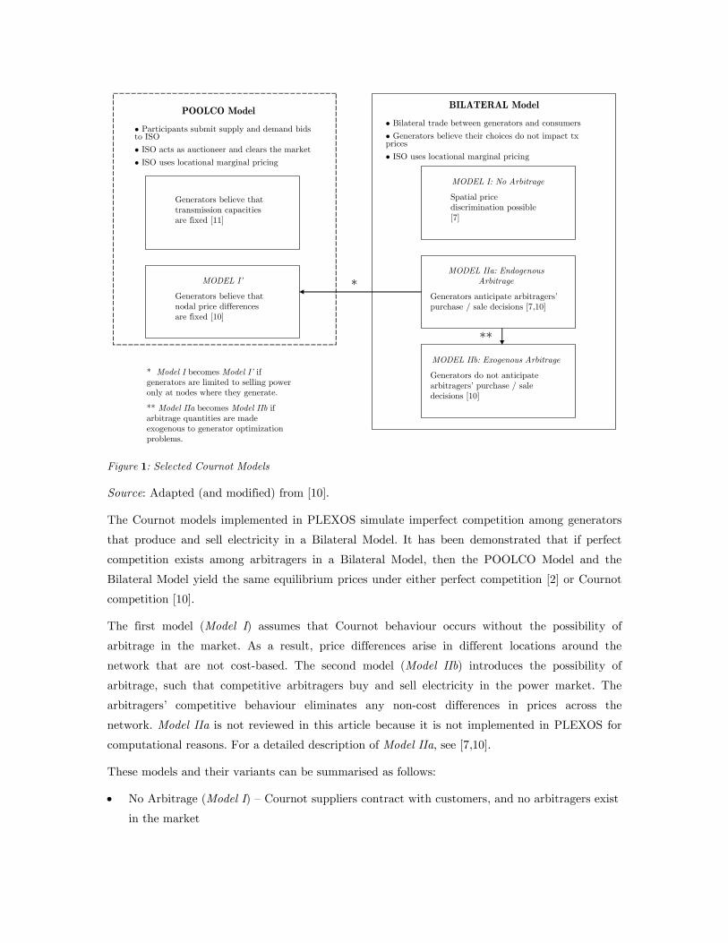
Figure 1 illustrates how these models relate to each other, as well as to several POOLCO models.

7

Generators believe that transmission capacities are fixed [11]

MODEL I’

Generators believe that nodal price differences are fixed [10]

POOLCO Model

• Participants submit supply and demand bids to ISO

• ISO acts as auctioneer and clears the market

• ISO uses locational marginal pricing

MODEL IIa: Endogenous Arbitrage

Generators anticipate arbitragers’ purchase / sale decisions [7,10]

BILATERAL Model

• Bilateral trade between generators and consumers

• Generators believe their choices do not impact txprices

• ISO uses locational marginal pricing

MODEL IIb: Exogenous Arbitrage

Generators do not anticipate arbitragers’ purchase / sale decisions [10]

MODEL I: No Arbitrage

Spatial price discrimination possible [7]

*

**

* Model I becomes Model I’ if generators are limited to selling power only at nodes where they generate.

** Model IIa becomes Model IIb if arbitrage quantities are made exogenous to generator optimization problems.

Figure 1: Selected Cournot Models

Source: Adapted (and modified) from [10].

The Cournot models implemented in PLEXOS simulate imperfect competition among generators

that produce and sell electricity in a Bilateral Model. It has been demonstrated that if perfect

competition exists among arbitragers in a Bilateral Model, then the POOLCO Model and the

Bilateral Model yield the same equilibrium prices under either perfect competition [2] or Cournot

competition [10].

The first model (Model I) assumes that Cournot behaviour occurs without the possibility of

arbitrage in the market. As a result, price differences arise in different locations around the

network that are not cost-based. The second model (Model IIb) introduces the possibility of

arbitrage, such that competitive arbitragers buy and sell electricity in the power market. The

arbitragers’ competitive behaviour eliminates any non-cost differences in prices across the

network. Model IIa is not reviewed in this article because it is not implemented in PLEXOS for

computational reasons. For a detailed description of Model IIa, see [7,10].

These models and their variants can be summarised as follows:

• No Arbitrage (Model I) – Cournot suppliers contract with customers, and no arbitragers exist

in the market

8

• Arbitrage – Cournot suppliers contract with customers, and competitive arbitrage forces

nodal price differences to equal the transmission cost

Stackelberg Conjecture – Endogenous Arbitrage (Model IIa – not presented) –

suppliers expect that arbitragers will adjust their purchases / sales in the market in

response to changes in supplier decisions

Cournot Conjecture – Exogenous Arbitrage (Model IIb) – suppliers make output and

price decisions under the assumption that arbitragers will not change their purchases

/ sales at each node

IIIC: Common Modelling Aspects

Models I, IIa, IIb include common assumptions regarding: i) transmission, ii) producers, and iii)

consumers. They are also characterised by the same form of solution. The existence of exogenous

arbitrage is unique to Model IIb. This section provides a detailed description of each of the

common model components.

IIIC.1: Transmission

IIIC.1.a: Description of the Network Model

The electricity network is modelled with a graph that uses a finite set of nodes (N) and a finite

set of directed arcs (A). In general, constraints on transmission are represented by a finite number

of linear inequalities. For purposes of the models, the constraints are limited to i) constraints on

the transmission capacities of any of the arcs, or reverse arcs, in K, and to ii) constraints on flow

balance.

The models use Kirchhoff’s laws and Power Distribution Factors (PDFs) to implement a

linearized DC network flow model [13]. A PDF represents the MW increase in flow resulting from

1MW of injection at an arbitrary hub, node H, and 1MW of power withdrawal at node i, due to

Kirchhoff’s laws. Under a linearized DC model, power is analogous to current, such that power

flows satisfy analogies to Kirchhoff’s Current Law and Kirchhoff’s Voltage Law. For any physical

network and an assumed set of network injections and withdrawals, these laws uniquely

determine the flows – unlike a ‘transshipment network’, in which discretion generally exists in

regard to the ‘routing’ of the network flows.

For example, consider a three-node (triangular) network in which each pair of nodes is connected

directly by a line with an electrical reactance of 2.5. By Kirchhoff’s laws, an injection of 10MW at

node 3 and a 10MW withdrawal at node 1 will result in the following power flows:

9

• 3.33MW from node 3 to node 2;

• 3.33MW from node 2 to node 1; and

• 6.67MW from node 3 to node 1.

These flows satisfy Kirchhoff’s Current Law since net flow into each node is zero, and they also

satisfy Kirchhoff’s Voltage Law since the net drop around any loop in the network is zero. In a

linearized DC load flow model, the change in voltage angle over an arc is proportional to the

product of the power flow and the reactance, e.g. proceeding around the voltage loop for the

previous example, i.e. 3-2-1-3, gives a net voltage drop of 2.5 x (3.33) + 2.5 x (3.33) + 2.5 x (-

6.67) = 0. An example of a PDF for a triangular network, with node 3 as the hub node, gives

PDFik = -.33 for node i = 1 and the arc k in the direction from node 1 to node 2.

Since the Kirchhoff equations that determine flows in the DC model are linear, the principle of

superposition applies; therefore, the flows induced by an injection of x at node i and a withdrawal

of x at node j equal the sum of the flows induced by injecting x at node i and withdrawing x at

the hub, node H, plus the flows induced by injecting x at node H and withdrawing x at node j.

Due to the linearity of the DC network approximation, all generation is notionally routed through

node H. The linearity property also implies that the choice of the hub node is arbitrary.

IIIC.1.b: Independent System Operator (ISO)

The ISO, by assumption, rations scarce interface capacity to maximize the value of transmission

services that it provides to the market. Equivalently, the ISO maximizes its profit from selling

transmission services (yi) to the market given the transmission fees (wi) that it charges to

producers (and arbitragers in Model IIb) and given interface constraints.

For transmission services, yi > 0 implies a net flow into node i while yi < 0 implies a net flow

from node i. The transmission fee is the cost that a producer (or arbitrager) pays the ISO for the

(notional) transmission of power from node H to node i. This assumption is also equivalent to a

competitive market for transmission rights. Further, the ISO maximizes its profit under the

assumption that it cannot strategically manipulate the fees that it charges for transmission

services.

In the models, the following notation is used for transmission:

• set of transmission nodes N.

• set of transmission arcs A.

• set of transmission interfaces K.

• transmission capacity on arc k . kT+

• transmission capacity on arc k in the reverse direction . kT−

• transmission (MW) from the hub node (H) to node i . iy

10

• power distribution factor for node i on arc k, PDFik.

representing the MW increase in flow resulting from

1MW of injection at node H and 1 MW of power

withdrawal at node i, due to Kirchhoff’s laws.

• transmission fee for transport from node H to i wi.

• price at the hub, node H pH.

IIIC.2: Consumers

Consumers at node i consume qi MW such that the price at node i (pi) is related linearly to

consumption by the nodal demand function:

(1) . 0 0 0( ) ( / )i i i i i ip q P P Q q= −

In the demand function, is the vertical intercept, and is the horizontal intercept. The use

of a linear demand function allows for the use of a Linear Complementarity or Quadratic Problem

(LCP or QP) formulation in the model. The use of a non-linear demand function would result in

a Non-linear Complementarity Problem (NCP), which is, in general, more difficult to solve.

0iP 0

iQ

IIIC.3: Producers

Each individual producer :f f F∈ is located at a node. A producer has a generation capacity

(MW) of Gif, and its generation (MWh) at node i is represented by gif.

A producer maximizes its profit, i.e. revenues less costs, under an assumption of imperfect

competition. The imperfect competition is modelled as Cournot behaviour with respect to sales in

the power market. A producer has the option to sell its generation at any node; therefore, the

sales at node i by producer f are sif. Producer revenue is the product of sales at a node and the

nodal price, summed across all nodes at which sales occur. The production cost possesses two

components: producer marginal production cost (Cif) and the transmission fee (wi). The

constraints on the producer are i) generation station capacity, ii) production and sales balance,

and iii) nonnegativity of both production and sales.

A critical assumption of the models is that producers do not anticipate the impact of their output

decisions on transmission congestion and prices. This assumption, therefore, eliminates the

situations in which producers manipulate transmission in a strategic manner to their benefit. This

assumption diverges from the assumptions of the models in [3,11], in which producers anticipate

(correctly) the effect of their decisions on transmission limits and on the resulting transmission

prices.

The disadvantage of the assumption is that it does not allow for the possibility that, in reality,

producers recognise the impact of their decisions on transmission prices. The advantage, however,

is that the models are solvable for realistically large networks. The primary reason for this

improvement in solvability is that the representation of producers’ expectations - of their output

11

decisions on transmission prices - requires that each producer’s optimization problem includes the

Karush-Kuhn-Tucker (KKT) conditions of the ISO’s optimal power flow problem. The resulting

mathematical program is highly non-convex and may possess multiple, local optima.

Consequently, this simplifying assumption represents a tradeoff between a possibly more realistic

representation of producer behaviour and computability.

IIIC.4: Solution

Given the assumptions on market design and market participant interaction, each model

determines a market equilibrium. An equilibrium is defined as a set of generator outputs,

consumer demands, prices, transmission flows, and arbitrage quantities (Model IIb) that satisfy

the market participants’ profit maximization conditions and market-clearing condition. A solution

to each model that satisfies these conditions possesses the Nash equilibrium property – no

participant has the incentive to unilaterally deviate from its equilibrium choices.

IIID: The Models

This section contains a detailed description of the Cournot models implemented in PLEXOS.

IIID.1: Cournot Model I: No Arbitrage

Model I is derived from [7]. An equivalent model is developed by [15] and includes the possibility

of generation capacity expansion. This model proves existence and uniqueness of a solution by

variational inequality methods. In addition, [10] proves existence and uniqueness using

complementarity methods.

IIID.1.a: Description and Model-specific Assumptions

In Model I, power flows on a linearized DC network and the ISO allocates scarce transmission

capacity efficiently. Trade in the electricity market occurs consistent with the Bilateral Model,

such that producers, i.e. generators, contract directly with consumers for power supply. No

arbitragers exist in the market. Since no arbitrage occurs between locations in the network, the

Cournot assumption on generator behaviour enables non-cost based price differences to arise in

different locations across the network.

In summary, the following assumptions on producer, consumer, and transmission behaviour

characterise Model I:

• power flows over a linearized DC network;

• oligopolistic producers behave as Cournot suppliers in a Bilateral Model;

• transmission capacity is allocated efficiently; and

• arbitragers do not exist in the power market to eliminate non-cost price differences.

12

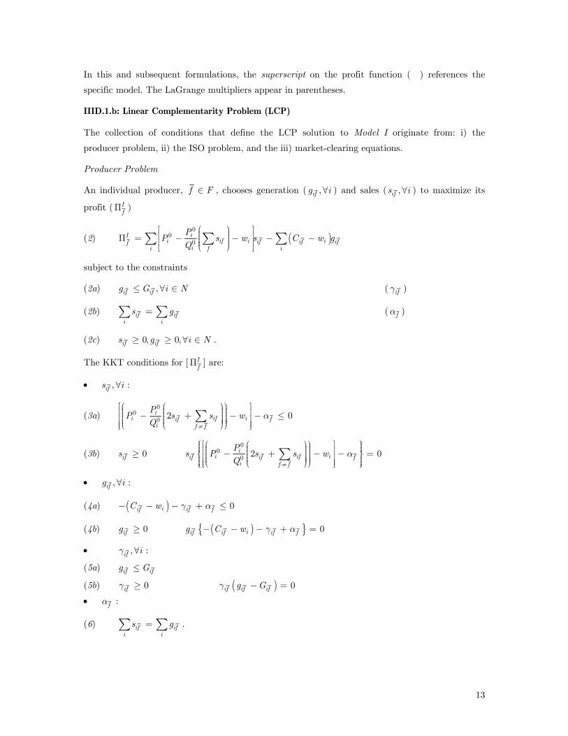
In this and subsequent formulations, the superscript on the profit function (�) references the

specific model. The LaGrange multipliers appear in parentheses.

IIID.1.b: Linear Complementarity Problem (LCP)

The collection of conditions that define the LCP solution to Model I originate from: i) the

producer problem, ii) the ISO problem, and the iii) market-clearing equations.

Producer Problem

An individual producer, f F∈ , chooses generation ( ,ifg ∀i ) and sales ( ,ifs ∀i ) to maximize its

profit ( If

Π )

(2) ( )0

00iI

i if i if if iffii f i

PP s w s C w

Q

⎡ ⎛ ⎞ ⎤⎟⎜⎢ ⎥⎟Π = − − − −⎜ ⎟⎜⎢ ⎥⎟⎜⎝ ⎠⎣ ⎦∑ ∑ ∑ i g

subject to the constraints

(2a) ,if ifg G i≤ ∀ ∈ N ( ifγ )

(2b) if ifi i

s =∑ ∑ g ( fα )

(2c) 0, 0,if ifs g i≥ ≥ ∀ ∈ N .

The KKT conditions for [ If

Π ] are:

• , :ifs i∀

(3a) 0

00 2 0i

i if iif fi f f

PP s s w

Qα

≠

⎡⎛ ⎛ ⎞⎞ ⎤⎟⎟⎜ ⎜⎢ ⎥⎟⎟⎜ ⎜− + − −⎟⎟⎜ ⎜⎢ ⎥⎟⎟⎟⎟⎜ ⎜⎝ ⎝ ⎠⎠⎢ ⎥⎣ ⎦∑ ≤

(3b) 0ifs ≥ 0

00 2 0i

i if iif if fi f f

Ps P s s w

Qα

≠

⎧ ⎡⎛ ⎛ ⎞⎞ ⎤ ⎫⎪ ⎪⎟⎟⎜ ⎜⎪ ⎪⎢ ⎥⎟⎟⎜ ⎜− + − −⎨ ⎬⎟⎟⎜ ⎜⎢ ⎥⎟⎟⎪ ⎪⎟⎟⎜ ⎜⎝ ⎝ ⎠⎠⎢ ⎥⎪ ⎪⎩ ⎣ ⎦ ⎭∑ =

• , :ifg i∀

(4a) ( ) 0iif if fC w γ α− − − + ≤

(4b) 0ifg ≥ ( ){ } 0iif if if fg C w γ α− − − + =

• , :if iγ ∀

(5a) if ifg G≤

(5b) 0ifγ ≥ ( ) 0if if ifg Gγ − =

• :fα

(6) if ifi i

s g=∑ ∑ .

13

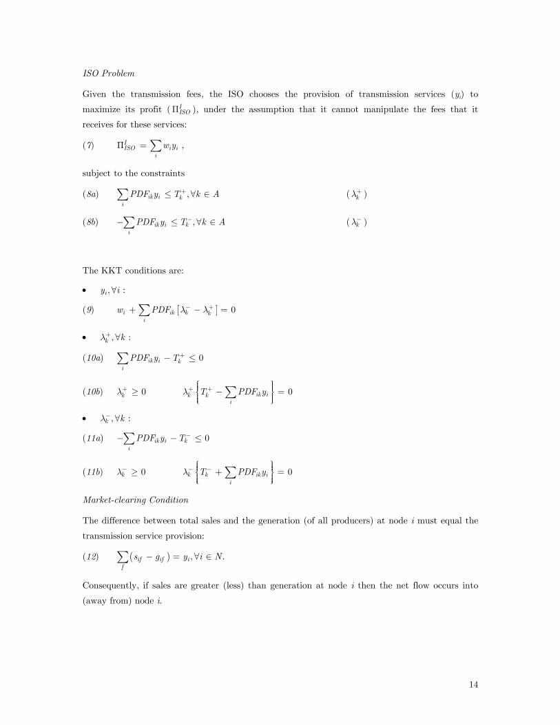
ISO Problem

Given the transmission fees, the ISO chooses the provision of transmission services (yi) to

maximize its profit ( ), under the assumption that it cannot manipulate the fees that it

receives for these services:

IISOΠ

(7) , IISO i i

i

w yΠ = ∑

subject to the constraints

(8a) ( ) ,ik i ki

PDF y T k A+≤ ∀ ∈∑ kλ+

(8b) ( ) ,ik i ki

PDF y T k A−− ≤ ∀∑ ∈ kλ−

The KKT conditions are:

• , :iy i∀

(9) [ ] 0i ik k ki

w PDF λ λ− ++ −∑ =

≤

• , :k kλ+ ∀

(10a) 0ik i ki

PDF y T+− ≤∑

(10b) 0kλ+ ≥ 0ik ik k

i

T PDF yλ+ +⎧ ⎫⎪ ⎪⎪ ⎪− =⎨ ⎬⎪ ⎪⎪ ⎪⎩ ⎭∑

• , :k kλ− ∀

(11a) 0ik i ki

PDF y T−− −∑

(11b) 0kλ− ≥ 0k k ik ii

T PDF yλ− −⎧ ⎫⎪ ⎪⎪ ⎪+ =⎨ ⎬⎪ ⎪⎪ ⎪⎩ ⎭∑

Market-clearing Condition

The difference between total sales and the generation (of all producers) at node i must equal the

transmission service provision:

(12) ( ) , .if if if

s g y i N− = ∀ ∈∑

Consequently, if sales are greater (less) than generation at node i then the net flow occurs into

(away from) node i.

14

Comments on LCP Solution

The LCP solution is obtained by solving (3-6), (9-11), and (12) simultaneously for the primal

variables. Although both the producer and the ISO problems naively assume that the wi are fixed,

the wi are variables in the LCP; the LCP solution yields the wi that clear the market for

transmission services.

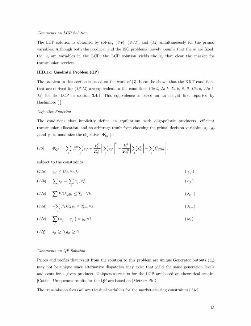
IIID.1.c: Quadratic Problem (QP)

The problem in this section is based on the work of [7]. It can be shown that the KKT conditions

that are derived for (13-14) are equivalent to the conditions (3a-b, 4a-b, 5a-b, 6, 9, 10a-b, 11a-b,

12) for the LCP in section 3.4.1. This equivalence is based on an insight first reported by

Hashimoto [ ].

Objective Function

The conditions that implicitly define an equilibrium with oligopolistic producers, efficient

transmission allocation, and no arbitrage result from choosing the primal decision variables, sif , gif

, and yi, to maximize the objective [ ]: IQPΦ

(13) 20 0

0 20 02 2

i iIQP i if if if if if

i ii f f f f

P PP s s s C g

Q Q

⎡ ⎤⎛ ⎞ ⎛ ⎞⎟ ⎟⎢ ⎥⎜ ⎜⎟ ⎟Φ = − − −⎜ ⎜⎟ ⎟⎢ ⎥⎜ ⎜⎟ ⎟⎜ ⎜⎝ ⎠ ⎝ ⎠⎢ ⎥⎣ ⎦∑ ∑ ∑ ∑ ∑ ,

subject to the constraints

(14a) ( ) , , .if ifg G i≤ ∀ f

f∀

ifγ

(14b) (, .if ifi i

s g=∑ ∑ fα )

(14c) ( ) ,ik i ki

PDF y T k+≤ ∀∑ .

∀

i

kλ +

(14d) ( ) , .ik i ki

PDF y T k−− ≤∑ kλ −

(14e) ( ) ( ) , .if if if

s g y− = ∀∑ iw

(14f) 0, 0.if ifs g≥ ≥

Comments on QP Solution

Prices and profits that result from the solution to this problem are unique.Generator outputs (gif)

may not be unique since alternative dispatches may exist that yield the same generation levels

and costs for a given producer. Uniqueness results for the LCP are based on theoretical studies

[Cottle]. Uniqueness results for the QP are based on [Metzler PhD].

The transmission fees (wi) are the dual variables for the market-clearing constraints (14e).

15

Example

[To be completed.]

IIID.2: Cournot Model IIb: Exogenous Arbitrage

This model is based on the work of [7,10]. The QP formulation is derived by Michael Blake

(Drayton Analytics Pty Ltd, Australia) and Benjamin Hobbs (The Johns Hopkins University,

U.S.A.).

IIID.2.a: Description and Model-specific Assumptions

In Model IIb, power flows on a linearized DC network, and an ISO allocates scarce transmission

capacity efficiently. Trade in the electricity market occurs consistent with the Bilateral Model,

such that producers, i.e. generators, contract directly with consumers for power supply. Unlike

Model I, however, arbitragers exist in the energy market. The arbitragers behave as price-takers,

given the prices at the various nodes in the network. With the possibility of arbitrage, only

transmission cost-based differences occur across nodes in the network in equilibrium.

The following assumptions on producer, consumer, and transmission behaviour characterise Model

IIb:

• power flows over a linearized DC network;

• oligopolistic producers behave as Cournot suppliers in a Bilateral Model;

• transmission capacity is allocated efficiently; and

• arbitragers exist in the power market and behave as price-takers.

Specific to this model, producers assume naively that they are able to affect prices in one location

without affecting prices at other locations in the network. In other words, producers simply

accept the arbitrage quantities as given in their profit maximization problems. This modelling

assumption is equivalent to a Cournot conjecture in relation to arbitrage quantities since the

latter are effectively exogenous to the producers’ decisions. This assumption leads to several

modelling simplifications that make computation tractable for large networks.

IIID.2.b: Linear Complementarity Problem (LCP)

The collection of conditions that define the LCP solution to Model IIb derives from: i) the

producer problem, ii) the ISO problem, iii) the arbitrager problem, and the iv) market-clearing

equations.

Producer Problem

16

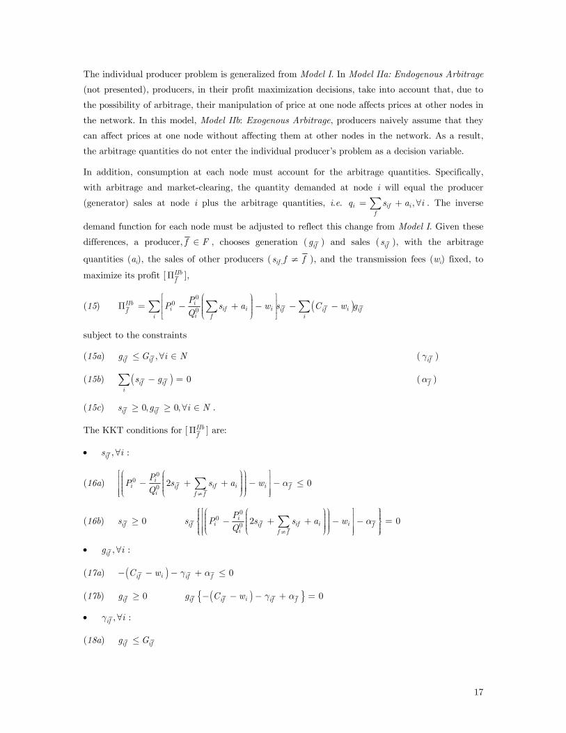
The individual producer problem is generalized from Model I. In Model IIa: Endogenous Arbitrage

(not presented), producers, in their profit maximization decisions, take into account that, due to

the possibility of arbitrage, their manipulation of price at one node affects prices at other nodes in

the network. In this model, Model IIb: Exogenous Arbitrage, producers naively assume that they

can affect prices at one node without affecting them at other nodes in the network. As a result,

the arbitrage quantities do not enter the individual producer’s problem as a decision variable.

In addition, consumption at each node must account for the arbitrage quantities. Specifically,

with arbitrage and market-clearing, the quantity demanded at node i will equal the producer

(generator) sales at node i plus the arbitrage quantities, i.e. . The inverse

demand function for each node must be adjusted to reflect this change from Model I. Given these

differences, a producer,

,i if if

q s a= +∑ i∀

f F∈ , chooses generation ( ifg ) and sales ( ifs ), with the arbitrage

quantities (ai), the sales of other producers ( ,ifs f f≠ ), and the transmission fees (wi) fixed, to

maximize its profit [ IIbf

Π ],

(15) ( )0

00iIIb

i if i i if if iffii f i

PP s a w s C w

Q

⎡ ⎛ ⎞ ⎤⎟⎜⎢ ⎥⎟Π = − + − − −⎜ ⎟⎜⎢ ⎥⎟⎜⎝ ⎠⎣ ⎦∑ ∑ ∑ i g

subject to the constraints

(15a) ,if ifg G i≤ ∀ ∈ N ( ifγ )

(15b) ( ) 0if ifi

s g− =∑ ( fα )

(15c) 0, 0,if ifs g i≥ ≥ ∀ ∈ N .

The KKT conditions for [ IIbf

Π ] are:

• , :ifs i∀

(16a) 0

00 2 0i

i if i iif fi f f

PP s s a w

Qα

≠

⎡⎛ ⎛ ⎞⎞ ⎤⎟⎟⎜ ⎜⎢ ⎥⎟⎟⎜ ⎜− + + − −⎟⎟⎜ ⎜⎢ ⎥⎟⎟⎟⎟⎜ ⎜⎝ ⎝ ⎠⎠⎢ ⎥⎣ ⎦∑ ≤

(16b) 0ifs ≥ 0

00 2 0i

i if i iif if fi f f

Ps P s s a w

Qα

≠

⎧ ⎡⎛ ⎛ ⎞⎞ ⎤ ⎫⎪ ⎪⎟⎟⎜ ⎜⎪ ⎪⎢ ⎥⎟⎟⎜ ⎜− + + − −⎨ ⎬⎟⎟⎜ ⎜⎢ ⎥⎟⎟⎪ ⎪⎟⎟⎜ ⎜⎝ ⎝ ⎠⎠⎢ ⎥⎪ ⎪⎩ ⎣ ⎦ ⎭∑ =

• , :ifg i∀

(17a) ( ) 0iif if fC w γ α− − − + ≤

(17b) 0ifg ≥ ( ){ } 0iif if if fg C w γ α− − − + =

• , :if iγ ∀

(18a) if ifg G≤

17

(18b) 0ifγ ≥ ( ) 0if if ifg Gγ − =

• :fα

(19) if ifi i

s g=∑ ∑

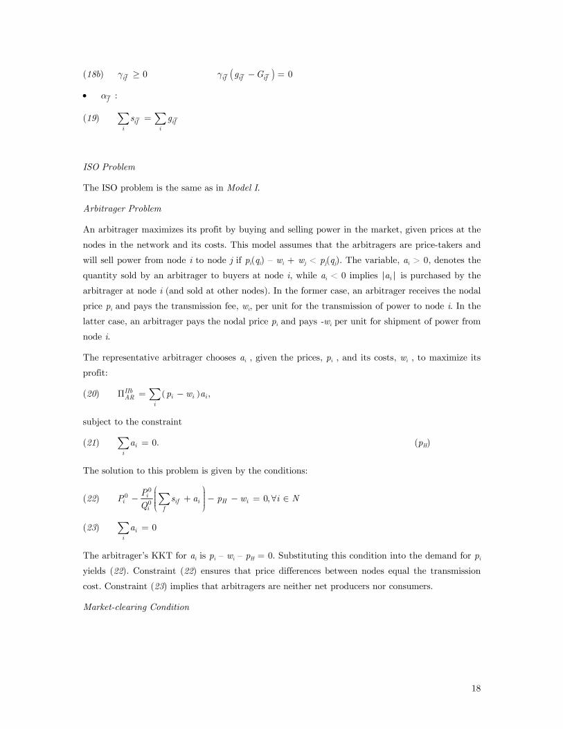
ISO Problem

The ISO problem is the same as in Model I.

Arbitrager Problem

An arbitrager maximizes its profit by buying and selling power in the market, given prices at the

nodes in the network and its costs. This model assumes that the arbitragers are price-takers and

will sell power from node i to node j if pi(qi) – wi + wj < pj(qj). The variable, ai > 0, denotes the

quantity sold by an arbitrager to buyers at node i, while ai < 0 implies ia is purchased by the

arbitrager at node i (and sold at other nodes). In the former case, an arbitrager receives the nodal

price pi and pays the transmission fee, wi, per unit for the transmission of power to node i. In the

latter case, an arbitrager pays the nodal price pi and pays -wi per unit for shipment of power from

node i.

The representative arbitrager chooses ai , given the prices, pi , and its costs, wi , to maximize its

profit:

(20) ( ) ,IIbi iAR

i

p w aΠ = −∑ i

subject to the constraint

(21) (p0.ii

a =∑ H)

The solution to this problem is given by the conditions:

(22) 0

00 0,i

i if i H ii f

PP s a p w i

Q

⎛ ⎞⎟⎜ ⎟− + − − = ∀⎜ ⎟⎜ ⎟⎜⎝ ⎠∑ N∈

(23) 0ii

a =∑

The arbitrager’s KKT for ai is pi – wi – pH = 0. Substituting this condition into the demand for pi

yields (22). Constraint (22) ensures that price differences between nodes equal the transmission

cost. Constraint (23) implies that arbitragers are neither net producers nor consumers.

Market-clearing Condition

18

The market-clearing condition must be modified to account for the possibility of arbitrage. Net

total sales at node i plus arbitrage sales at node i must equal the transmission service provision to

node i:

(24) ( ) , .if if i if F

s g a y∈

− + = ∀∑ i

Comments on LCP Solution

The LCP solution can be obtained by solving (16-19), (9-11), and (22-24) simultaneously for the

primal variables. Both the producers and the ISO assume that the wi are fixed. The wi, however,

are variables in the LCP, and its solution yields the wi that clear the market for transmission

services.

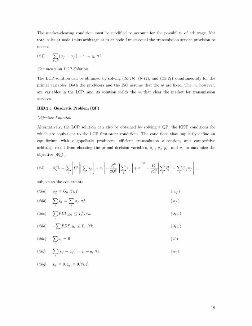
IIID.2.c: Quadratic Problem (QP)

Objective Function

Alternatively, the LCP solution can also be obtained by solving a QP, the KKT conditions for

which are equivalent to the LCP first-order conditions. The conditions that implicitly define an

equilibrium with oligopolistic producers, efficient transmission allocation, and competitive

arbitrage result from choosing the primal decision variables, sif , gif, yi , and ai, to maximize the

objective [ ]: IIbQPΦ

(25) 20 0

0 20 02 2

i iIIbQP i if i if i if if if

i ii f f f f

P PP s a s a s C g

Q Q

⎡ ⎤⎡⎛ ⎞ ⎤ ⎡⎛ ⎞ ⎤ ⎡ ⎤⎟ ⎟⎢ ⎥⎜ ⎜⎢ ⎥ ⎢ ⎥ ⎢ ⎥⎟ ⎟Φ = + − + − −⎜ ⎜⎟ ⎟⎢ ⎥⎜ ⎜⎢ ⎥ ⎢ ⎥ ⎢ ⎥⎟ ⎟⎜ ⎜⎝ ⎠ ⎝ ⎠⎢ ⎥⎣ ⎦ ⎣ ⎦ ⎣ ⎦⎣ ⎦∑ ∑ ∑ ∑ ∑ ,

subject to the constraints

(26a) ( ) , , .if ifg G i≤ ∀ f

f∀

ifγ

(26b) (, .if ifi i

s g=∑ ∑ fα )

(26c) ( ) ,ik i ki

PDF y T k+≤ ∀∑ .

.∀

.i

f

kλ +

(26d) ( ) ,ik i ki

PDF y T k−− ≤∑ kλ −

(26e) (β ) 0ii

a =∑

(26f) ( ) ( ) ,if if i if

s g y a− = − ∀∑ iw

(26g) 0, 0, , .if ifs g i≥ ≥ ∀

19

Comments on QP Solution

This model yields the same equilibrium prices, producer outputs, and profits as a POOLCO

Model with Cournot competition, in which an ISO buys power from producers and resells it to

consumers through the use of a centralised auction.

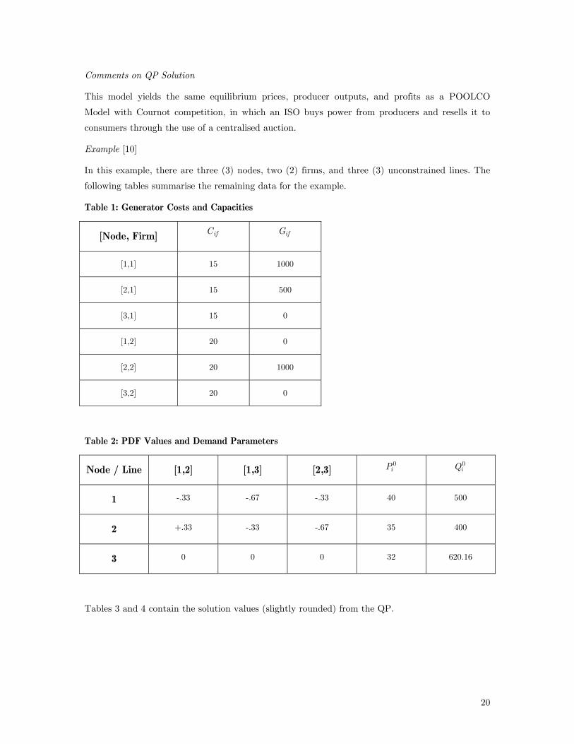
Example [10]

In this example, there are three (3) nodes, two (2) firms, and three (3) unconstrained lines. The

following tables summarise the remaining data for the example.

Table 1: Generator Costs and Capacities

[Node, Firm] ifC ifG

[1,1] 15 1000

[2,1] 15 500

[3,1] 15 0

[1,2] 20 0

[2,2] 20 1000

[3,2] 20 0

Table 2: PDF Values and Demand Parameters

Node / Line [1,2] [1,3] [2,3] 0

iP 0iQ

1 -.33 -.67 -.33 40 500

2 +.33 -.33 -.67 35 400

3 0 0 0 32 620.16

Tables 3 and 4 contain the solution values (slightly rounded) from the QP.

20

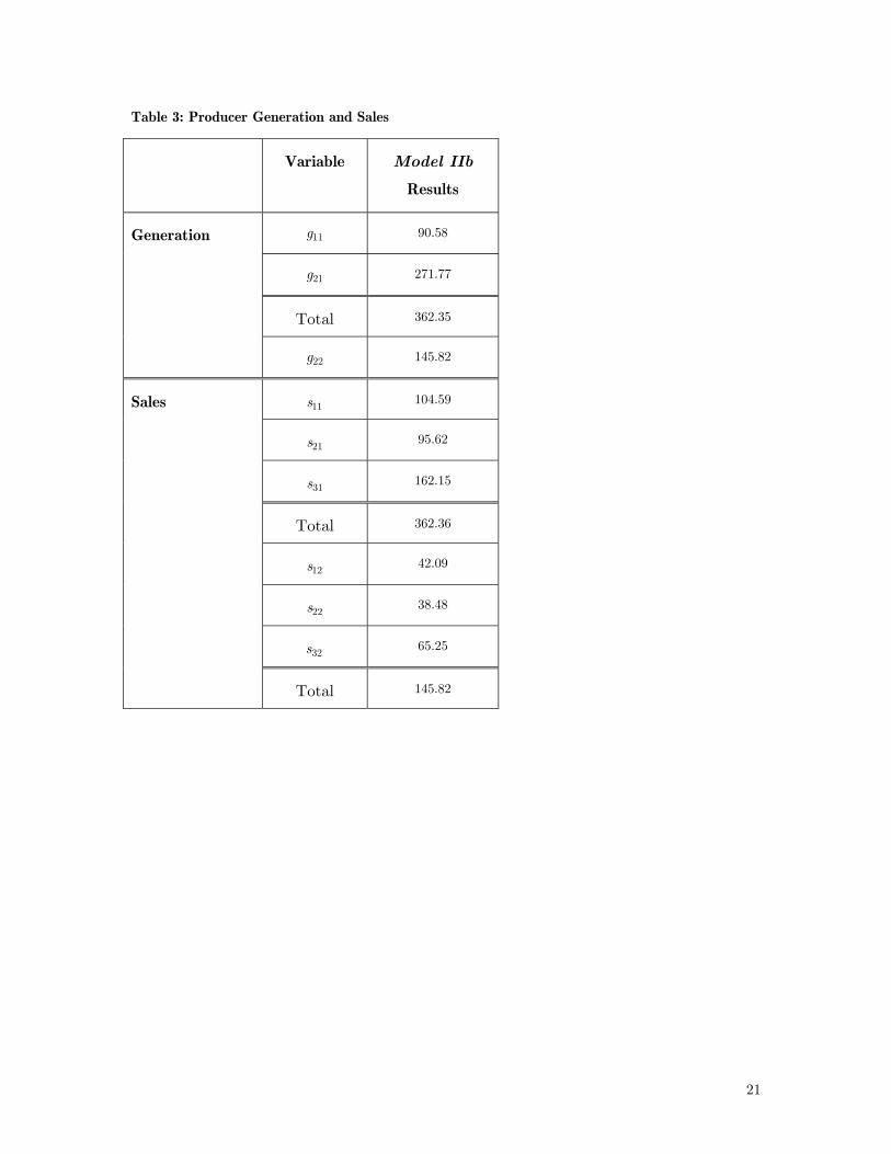
Table 3: Producer Generation and Sales

Variable Model IIb

Results

11g 90.58

21g 271.77

Total 362.35

Generation

22g 145.82

11s 104.59

21s 95.62

31s 162.15

Total 362.36

12s 42.09

22s 38.48

32s 65.25

Sales

Total 145.82

21

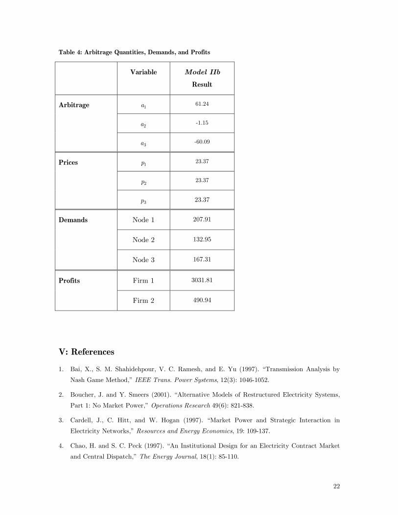
Table 4: Arbitrage Quantities, Demands, and Profits

Variable Model IIb

Result

1a 61.24

2a -1.15

Arbitrage

3a -60.09

1p 23.37

2p 23.37

Prices

3p 23.37

Node 1 207.91

Node 2 132.95

Demands

Node 3 167.31

Firm 1 3031.81 Profits

Firm 2 490.94

V: References

1. Bai, X., S. M. Shahidehpour, V. C. Ramesh, and E. Yu (1997). “Transmission Analysis by

Nash Game Method,” IEEE Trans. Power Systems, 12(3): 1046-1052.

2. Boucher, J. and Y. Smeers (2001). “Alternative Models of Restructured Electricity Systems,

Part 1: No Market Power,” Operations Research 49(6): 821-838.

3. Cardell, J., C. Hitt, and W. Hogan (1997). “Market Power and Strategic Interaction in

Electricity Networks,” Resources and Energy Economics, 19: 109-137.

4. Chao, H. and S. C. Peck (1997). “An Institutional Design for an Electricity Contract Market

and Central Dispatch,” The Energy Journal, 18(1): 85-110.

22

5. Chao, H. and S. C. Peck (1996). “A Market Mechanism for Electricity Power Transmission,”

Journal of Regulatory Economics, 10(1): 25-60.

6. Cottle, R., J. Pang, and R. Stone (1992). The Linear Complementarity Problem, Boston, MA:

Academic Press.

7. Daxhelet, O. and Y. Smeers (2001). “Variational Inequality Models of Restructured

Electricity Systems,” in Complementarity: Applications, Algorithms and Extensions (M.

Ferris, O. Mangasarian, and J. Pang, eds.), Dordrecht: Academic Publishers, 85-120.

8. Green, R. (1996). “Increasing Competition in the British Electricity Spot Market,” Journal of

Industrial Economics, 44: 205-216.

9. Hashimoto, H. (1985). “A Spatial Nash Equilibrium Model,” in Spatial Price Equilibria:

Advances in Theory, Computation, and Application, P. Harker (ed.), New York: Springer-

Verlag.

10. Hobbs, B. (2001). “Linear Complementarity Models of Nash-Cournot Competition in

Bilateral and POOLCO Power Markets,” IEEE Transactions on Power Systems, 16: 194-202.

11. Hobbs, B., C. Metzler, and J. Pang (2000). “Strategic Gaming Analysis for Electric Power

Networks: An MPEC Approach,” IEEE Transactions on Power Systems, 15(2): 638-645.

12. Hobbs, B. and R. Schuler (1985). “Assessment of the Deregulation of Electric Power

Generation Using Network Models of Imperfect Spatial Competition,” Papers of the Regional

Science Association, 57: 75-89.

13. Hogan, W. (1992). “Contract Networks for Electric Power Transmission,” Journal of

Regulatory Economics, 4(3): 211-242.

14. Metzler, C., B. Hobbs, and J. Pang (2002). “Nash-Cournot Equilibria in Power Markets on a

Linearized DC Network with Arbitrage: Formulations and Properties,” Networks and Spatial

Theory (forthcoming).

15. Metzler, C. (2000). Complementarity Models of Competitive Oligopolistic Electric Power

Generation Markets, Ph.D. Dissertation, Dept. of Mathematical Sciences, The Johns Hopkins

University, Baltimore, MD.

16. Oren, S. S. (1997). “Economic Inefficiency of Passive Transmission Rights in Congested

Electricity Systems with Competitive Generation,” The Energy Journal, 18(1): 63-83.

17. Ring, B. J. and E. G. Read (1996). “A Dispatch Based Pricing Model for the New Zealand

Electricity Market,” in Electricity Transmission Pricing and Technology, M. Einhorn and R.

Siddiqi, eds., Boston: Kluwer Academic Publishers.

18. Schweppe, F., M. Caramanis, R. Tabors, and R. Bohn (1988). Spot Pricing of Electricity,

Boston: Kluwer Academic Publishers, Appendix D.

23

19. Smeers, Y. and J. Wei (1997). “Do We Need a Power Exchange If There Are Enough Power

Marketers?,” CORE Discussion Paper 9760, Universite Catholique de Louvain.

20. Smeers, Y. and J. Wei (1997). “Spatially Oligopolistic Model with Opportunity Cost Pricing

for Transmission Capacity Reservations – A Variational Inequality Approach,” CORE

Discussion Paper 9717, Universite Catholique de Louvain.

21. von der Fehr, N. and D. Harbord (1993). “Spot Market Competition in the UK Electricity

Industry,” Economic Journal, 103: 531-546.

22. Wu, F. F. (1996). “Coordinated Multilateral Trades for Electric Power Networks,”

Department of Electrical Engineering, University of Hong Kong.

24