GCWerks for CRDS

GCWerks for CRDS

Copyright © 2019 GC Soft, Inc. All rights reserved.

GCWerks is a registered trademark of GC Soft, Inc.

Updated December 2019

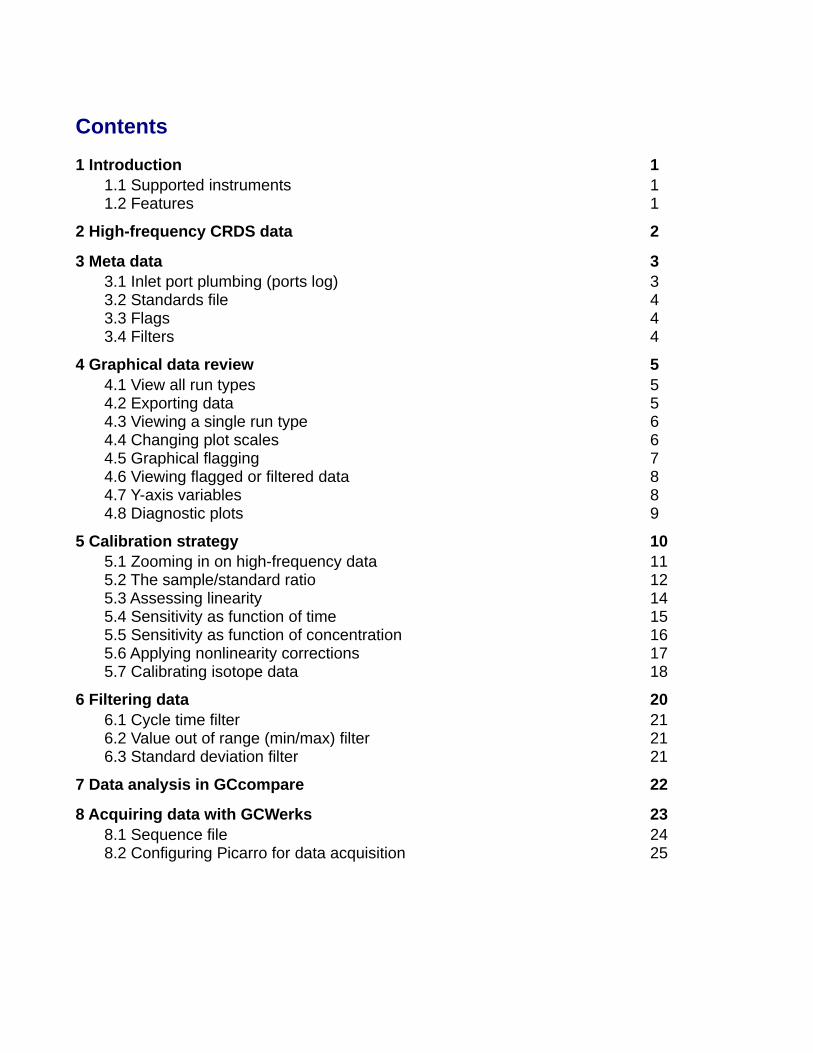
Contents

1 Introduction 11.1 Supported instruments 11.2 Features 1

2 High-frequency CRDS data 2

3 Meta data 33.1 Inlet port plumbing (ports log) 33.2 Standards file 43.3 Flags 43.4 Filters 4

4 Graphical data review 54.1 View all run types 54.2 Exporting data 54.3 Viewing a single run type 64.4 Changing plot scales 64.5 Graphical flagging 74.6 Viewing flagged or filtered data 84.7 Y-axis variables 84.8 Diagnostic plots 9

5 Calibration strategy 105.1 Zooming in on high-frequency data 115.2 The sample/standard ratio 125.3 Assessing linearity 145.4 Sensitivity as function of time 155.5 Sensitivity as function of concentration 165.6 Applying nonlinearity corrections 175.7 Calibrating isotope data 18

6 Filtering data 206.1 Cycle time filter 216.2 Value out of range (min/max) filter 216.3 Standard deviation filter 21

7 Data analysis in GCcompare 22

8 Acquiring data with GCWerks 238.1 Sequence file 248.2 Configuring Picarro for data acquisition 25

1 IntroductionGCWerks for CRDS is part of the GCWerks product family for greenhouse gas measurements, with the same software interface for GC, GC/MS and CRDS measurements.

This document provides an overview of GCWerks for CRDS capabilities, whether importing existing data or acquiring data from the instrument. For more details see the online documentation at http://gcwerks.com.

1.1 Supported instruments

GCWerks acquires or imports data from leading instrument manufacturers. It shields the userfor the specifics of each manufacturer's data formats and variable naming conventions, providing a uniform structure across manufacturers and models. Supported instruments include:

• Picarro: Acquires or imports data from the latest Picarro concentration or isotope analyzers, such as the G2401. Imports data from the older Picarro G1301 analyzer.

• LI-COR: Acquires or imports data from the LI-7810 CH4 analyzer or the LI-7815 CO2 analyzer.

• Los Gatos Research: Acquires or imports data from the latest LGR analyzers.

• Aerodyne: Imports data from Aerodyne QC laser analyzers.

• Valco valves for automation of sampling.

1.2 Features

• A single Linux system can acquire data from all instruments at a remote site (CRDS, GC, GC/MS), providing a secure point of access to remote instruments.

• Automation for reliable unattended operation, with email notification of user-defined alarm conditions

• Easy handling of large volumes of data, fast interactive graphics for years of data

• Uniform control of addition hardware for sampling (Valco valves, inlet sample pressure and temperature, etc.).

• Team access to a single multi-user Linux server data from all instruments.

• Imported or acquired data stored as binary strip-charts over 30 times smaller than hourly Picarro files (for fast data processing and copying over the Internet).

• Calculates results based on periodic standard measurements

• Nonlinearity and other diagnostics

• Graphical data flagging

GCWerks for CRDS - 1

http://gcwerks.com/

2 High-frequency CRDS dataCRDS data which are imported or acquired directly by GCWerks are stored in binary strip-charts. These strip-charts include all the relevant data from the instrument, and any additional data acquired by GCWerks (inlet temperature, pressure, ambient temperature, weather station data, etc.).

Files are named by GMT date and time. A new file is created each time the inlet port has changed, with normally a maximum of 1 hour of data in each file. All files for one year are stored in a single directory (e.g. victorville-picarro/13/strip-chart/) and are named as follows:

yymmdd.hhmmss.port - imported files

yymmdd.hhmmss.type.port - files acquired by GCWerks

Imported files include the inlet port number in the file name. Files acquired directly by GCWerks also include the run type (air, std, tank, etc.) in the file name.


Figure 1: Strip-chart showing high-frequency CRDS data

3 Meta data

3.1 Inlet port plumbing (ports log)

The ports log describes what is on each inlet for each time period.

# Date Time Port Tank Regulator Type Reject Bin#------ ---- ---- -------- --------- ---- ------ ---110101 0000 1 90m - air 1110101 0000 2 90m - air 1110101 0000 3 50m - air 1#110101 0000 4 JB03331 - cal 10110101 0000 5 JB03203 - std 10#130601 0000 5 JB03205 - std 10

The 'Type' column specifies the run type. Common types are:

• air: ambient air

• cal: calibration tanks

• std: one of the cal tanks, used as the reference to calibrate the data

• zero: zero gas

• tank: tank being calibrated

One of the cal tanks (usually near ambient) is defined as the reference standard which is used to calibrate the data. If there are two near-ambient cal tanks, either one can be used at any time as the standard to calculate results.

The 'Reject' column specifies the number of minutes to reject after switching to a new inlet. This is normally longer for calibration tanks (10 minutes in the example above). If the previous inlet has a greater reject time than the new inlet (air following cal in the example above), then the longer reject time is used for the new inlet (this may be disabled by setting “crds-reject-after: 0” in gcwerks.conf).

The 'Bin' column affects the time-interval over which data are averaged. If set to 1, the air data are binned in even time interval (e.g. 00-01, 01-02, for hourly means); 0000-0020, 0020-0040 for 20-minute means, etc.). This is most useful when there is a single air inlet. (1-minute data are always binned in even minutes).


3.2 Standards file

Calibration tank concentrations are specified in the standards file. The header defines the columns in the file.

tank co2 ch4#JB03331 393.392 1858.17JB03203 393.169 1871.4

3.3 Flags

Section 4.5 describes graphical data flagging. This is useful for flagging occasional outliers orgroups of outliers.

For flagging very long time periods, months or years, it is better to enter the flag manually in the “range flags file”. This specifies the date range, inlet port number and species:

##date time date time port gas flag#----- ---- ------ ---- ---- --- ----120101 0000 120607 2000 4 all F

This can also be useful for ongoing problems, by setting the ending date into the future, so that newly acquired data are automatically flagged (for the specified inlet port) until the problem is resolved.

3.4 Filters

Filters specify conditions for automatically rejecting bad data, for example cavity temperature or pressure out of range. Statical filters may also be used to eliminate outliers from the high-frequency data before averaging.


4 Graphical data reviewMean data may be viewed graphically in a number of ways. The displayed mean may be changed by selecting 60 min, 20 min, 5 min or 1 min on the lower left-hand corner.

4.1 View all run types

Any of the raw or calculated data may be displayed for any run type (air, cal, tank, etc.) simultaneously in different colors.

4.2 Exporting data

The report below the time-series plot is displayed with View > report. For any displayed mean (5 minute, 20 minute, etc.) the listed data may be saved to a file with File > Saveas.... To automate exporting or for more control over exported columns and data, see exporting results on the GCWerks website documentation.


Figure 2: Reviewing air data (blue), ambient-level and high calibration tanks as 20 minute averages. The data listing below corresponds to the plotted data.

4.3 Viewing a single run type

When viewing an individual run type (air, cal, tank, etc.), each inlet port is plotted in a differentcolor. The list at left shows what is plumbed on each inlet port for each time period, and allows selecting data to plot or export from the report listing.

4.4 Changing plot scales

Dragging the cursor on the time-series plot (left mouse button) zooms only the time-axis, with the y-axis self-scaled. This is useful as the y-axis will always scale properly for any displayed time period, gas, or y-axis variable. To disable this zoom mode and allow a rectangle zoom box (x and y zoom), un-check x-zoom only on the plot menu.

The left/right and up/down arrow buttons on the axes may also be used to change the the plotscales. Press the left mouse button on an arrow to move the view. Press the right mouse button to compress or stretch the scale.


Figure 3: Air data with each inlet in a different color.

4.5 Graphical flagging

The 1-minute data may be flagged graphically, with the resulting flags applying to the 5-minute, 20-minute and 60-minute means. To select a single point to flag, hold down the SHIFT key and click on the point. Click on the point again to un-select it. To flag a group of points, hold down the SHIFT key and use the zoom box as shown in Figure 4. To clear all selected points, press clear.

The default flag is the 'F' flag, which flags a point as a flyer to exclude from the calculated results. The 'U' flag may be used to unflag a point. Press apply flags to flag the currently selected points for the displayed gas.

After applying flags in this way, select update > update all to re-calculate mean data with the new flags applied. If flagging only the latest year, use select update > update latest year.


Figure 4: SHIFT-zoom box to select points to flag graphically. Only 1-minute data may be flagged.

4.6 Viewing flagged or filtered data

When all the points in a mean (5-minute, 20-minute, etc.) are flagged or filtered (or fewer thana minimum number of points remain), the means are not normally displayed. They may be displayed with the following options:

Options > show flagged points ('F')

Options > show filtered points ('*')

Options > show rejected points ('x') - only plotted for 1-minute data

(The rejected points are in the transient period after switching to a new inlet port, as specified in the 'Reject' column in the ports.log.)

4.7 Y-axis variables

For each y-axis variable, the displayed mean may be changed by selecting 60 min, 20 min, 5min or 1 min on the lower left-hand corner. The y-axis variables are:

• measured (dry): Measured concentration, corrected for water (and matrix effects for isotope analyzers).

• measured (wet): Measured concentration, not corrected for water for matrix effects (not available for all species or analyzer models).

• stdev: standard deviation of the mean of the high-frequency raw data for each species

• N: the number of high-frequency data points in each mean

• N filtered: the number of high-frequency data points filtered or flagged for each mean

• C (drift corrected) = Cdrift: single point calibration, using linear interpolation of response from bracketing standard measurements.

• C (nonlin corrected): single point calibration with additional correction for concentration dependent response (nonlinearity)

• sensitivity = dry / Ctank: instrument response divided by tank concentration (useful to plot for calibration tanks).

• drift corrected sensitivity = Cdrift / Ctank: the drift-corrected concentration for calibration tank measurements divided by the tank concentration.

• seconds / cycle: The number of seconds for a complete (Picarro) measurement cycle(e.g. CO2, CH4, CO, H2O on a G2401).

• cavity press, cavity temp, etc: all other instrumental data


4.8 Diagnostic plots

Any of the Picarro parameters may be plotted to diagnosing instrument performance over time. Below is a plot of “seconds / cycle” for a Picarro G2301. This is the number of seconds required for a complete measurement cycle (CO2, CH4, H2O) and should typically be below 5seconds. This is an important diagnostic of laser performance. Values above 5 seconds, or large variability, indicate need for service (usually remote calibration).


Figure 5: The number of seconds required for a complete measurement cycle (CO2, CH4, H2O on this G2301). This should be typically below 5 seconds.

5 CalibrationGCWerks typically uses a single, near-ambient standard to track drift in instrumental response. Results can be corrected for this drift by either the difference between the standard’s measured and assigned value, or the ratio of the standard’s measured to assignedvalue. In general it appears that relatively small peaks (such as CO on a Picarro 2401 or 13Cisotope measurements) are better corrected by difference, as drift in the spectroscopic baseline fitting offset likely dominates. For large peaks (such as CO2 or CH4) it appears that percentage drift dominates (mostly likely in the pressure sensor) and ratio correction is better. Examples of this are shown in the next section below.

In addition to the single point calibration which corrects for drift in instrumental response, GCWerks has the capability to apply a nonlinearity correction, which can be determined with a single high standard or a range of standards. For instruments such as Picarro, which are well pressure and temperature controlled, this nonlinearity correction tends to be small and stable over long periods of time. Examples of this using a suite of ICOS tanks are shown in the sections that follow. This is not the case for instruments such as LGR, where at least two standards (ambient and high) need to be run frequently to track both drift and linearity changes (as cavity temperature and pressure drift).


5.1 Drift correct by ratio or difference?

By default GCWerks corrects for instrument drift based on the ratio of the measured standard value to the assigned value. This can be changed from ratio to difference for a given species by the gcwerks.conf variable “drift-diff”, for example CO measurements on a Picarro 2401:

drift-diff: co

Figure 6 shows Picarro 2401 CO measurements of two near ambient standards (111.62 ppb and 235.35 ppb) and a high standard (1318.11 ppb).


Figure 6: Low and high CO calibration tanks.

Figure 7 shows the same data plotted as ratio to mean (top panel) and difference from mean (bottom panel). From this it is clear that the difference from mean is needed to track drift for CO on a Picarro 2401.

GCWerks does the drift correction based on difference as described below:

Cdrift = M + (Cstd - Mstd)

Cdrift = drift-corrected concentration (single-point calibration)

Cstd = assigned standard concentration

M = measured (dry)

Mstd = measured (dry) time-interpolated from adjacent standard measurements


Figure 7: CO calibration tanks plotted as (Top) ratio to the tank’s mean and (Bottom) difference from the tank’s mean.

Figure 8 shows the same data for CO2, with two near ambient standards (395.20 ppm and 387.68 ppm) and a high standard (869.57 ppm). In this case it is clear that CO2 is better drift corrected by ratio, rather than difference.

GCWerks does the drift correction based on ratio as described below:

Cdrift = M x Cstd / Mstd

Cdrift = drift-corrected concentration (single-point calibration)

Cstd = assigned standard concentration

M = measured (dry)

Mstd = measured (dry) time-interpolated from the adjacent standard measurements


Figure 8: CO2 calibration tanks plotted as (Top) ratio to the tank’s mean and (Bottom) difference from the tank’s mean.

5.2 Zooming in on high-frequency data

Use View > stripchart to display the strip-chart, then click (or drag the cursor) on any point on the time-series to view the corresponding high-frequency data. Select 60 min to see the mean of the full standard or tank measurement (assuming measurements are 60 minutes or shorter).

Time=0 on each strip-chart corresponds to change of inlet port, making it easy to asses the transient period (to reject after an inlet change). In the example below, "reject minutes" in theports.log has been set to 10 minutes so the first 10 minutes are excluded from the mean. Theremaining data (between the vertical black lines) are averaged. Standard measurements used to calibrate the data are always averaged for the full measurement time, after the transient period has been rejected.


Figure 9: The high-frequency data between the vertical lines below correspond to the mean pointed toby the cursor above.

5.3 The sample/standard ratio

To take out time-dependent drift in instrument response, the ratio is taken of any measurement to the time interpolation of the neighboring standards.

Figure 4 shows two near-ambient calibration tanks run daily over several months on a Picarro2301. The striking feature is the coherent pattern of instrumental response between the two tanks. Either of these two calibration tanks may be used as the reference standard (this is done by assigning it type 'std' in the ports.log). In this case the tank plotted in red was designated as the 'std'. The red points on the bottom panel show the std/std ratio, which is the ratio of each std to the time interpolation of its neighboring standards. The orange points show the tank/std ratio for the cal tank.

.


Figure 10: The bottom panel shows the sample/standard ratio calculated by linear interpolation from the neighboring standard measurements.

Below is an example from LGR showing two near-ambient tanks with a significant N2O response drift over a two month period. Drift correction by linear interpolation here results in standard deviations of about 0.017% for the std/std ratio and 0.012% for the tank/std ratio.


Figure 11: LGR N2O response for two tanks (top), and sample/standard ratio determined by time interpolation from neighboring daily standards (bottom).

5.4 Assessing linearity

Linearity is assessed by measuring tanks with a range of concentrations. For a linear instrument the response/concentration ratio (sensitivity) should be independent of concentration. Of importance is how the tanks of high and low concentrations are prepared (in particular are high tanks spiked with compounds in roughly their naturally-occurring isotopic ratios?) and how the tanks are assigned values. The linearity of the instrument used to assign values to the calibration tanks must be independently verified.

Figure 12 shows calibration tanks spanning a range of concentrations measured approximately monthly over a 9 month period. The Picarro responses are plotted as ratios to the standard (with the standard defined at y=1.0).


Figure 12: Calibration tank measurements plotted as ratio to the standard . In blue are the daily standard measurements (at y=1.0 by definition).

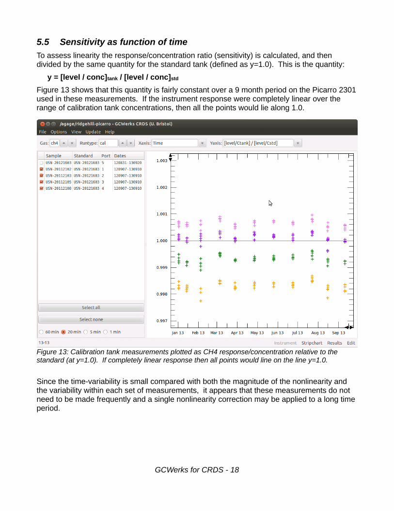
5.5 Sensitivity as function of time

To assess linearity the response/concentration ratio (sensitivity) is calculated, and then divided by the same quantity for the standard tank (defined as y=1.0). This is the quantity:

y = [level / conc]tank / [level / conc]std

Figure 13 shows that this quantity is fairly constant over a 9 month period on the Picarro 2301used in these measurements. If the instrument response were completely linear over the range of calibration tank concentrations, then all the points would lie along 1.0.

Since the time-variability is small compared with both the magnitude of the nonlinearity and the variability within each set of measurements, it appears that these measurements do not need to be made frequently and a single nonlinearity correction may be applied to a long time period.


Figure 13: Calibration tank measurements plotted as CH4 response/concentration relative to the standard (at y=1.0). If completely linear response then all points would line on the line y=1.0.

5.6 Sensitivity as function of concentration

When the data in Figure 13 are plotted a function of concentration we see a fairly significant slope of about 0.3% over the range 1600 to 2200 ppb.

Here it is clear that a single fit of the calibration tanks measured over the 9 month period is sufficient to correct for the nonlinearity. This fit is relative to the standard's response, so values above 1.0 indicate a greater sensitivity than at the concentration of the standard. This can be fitted as a simple slope over a limited concentration range or as a quadratic as shown above.


Figure 14: Calibration tank measurements plotted as CH4 response/concentration relative to the standard (at y=1.0) versus x=tank concentration.

For CO2 the measured nonlinearity is an order of magnitude smaller, and it may not be necessary to correct for over a limited concentration range.

5.7 Applying nonlinearity corrections

Details of fitting and applying nonlinearity corrections are described on the GCWerks website documentation under calculating results / nonlinearity correction.


Figure 15: Calibration tank measurements plotted as CO2 response/concentration relative to the standard (at y=1.0) versus x=tank concentration.

5.8 Calibrating isotope data

Figure 16 shows an example of Picarro G2132-i δ13C CH4 data. δ13C is defined as:

δ13C = [ (13C/12C)/REF – 1] x 1000

The top panel of the figure shows the measured δ13C for air (blue), working standard (green) and periodic calibration tanks (orange). The bottom panel shows the sample/standard ratio interms of (δ + 1000):

sample/standard = (13C/12C)sample / (13C/12C)standard


Figure 16: Picarro-reported δ13C CH4 values (top), and sample/standard ratio determined by time interpolation from neighboring standards (bottom).

The approach taken by GCWerks is to calibrate 13C and 12C independently, including any nonlinearity corrections, and then to compute a calibrated δ. This takes into consideration

that 13C is a small peak (about 1% of 12C) and vulnerable to small offsets in spectroscopic

baseline fitting, resulting in a potentially large nonlinearity compared with 12C. A nonlinearity in terms of δ would be much more complicated mathematically as the absolute peak size (e.g.12C concentration) must also be part of the function.


6 Filtering dataA number of filters are automatically applied to the high-frequency data before the mean is taken. These are configured in the gcwerks.conf file and the default settings are described in the sections below. Filter results are shown on the high-frequency strip-chart with a letter code for each filtered or flagged point. The codes are:

P = cavity pressure out of range T = cavity temperature out of range W = water value too high C = cycle time too high S = standard deviation filtered (for measured compound or water)

Flagged or rejected data are also displayed with letter codes.

F = flagged data x = rejected data (transient period after switch to a new inlet port)

Notes: Filters are not applied to rejected ('x') or flagged ('F') data. Any filter may be turned off by changing its setting to 0.


Figure 17: Strip-chart corresponding to cursor in top panel, showing filtered cal tank points (here labled 'S ' and 'P') and initial rejection period (labeled 'x').

The number of points filtered or flagged for each mean point (5-min, 20-min, etc.) is displayedwith y=Nfiltered. To see means which have been completely flagged for filtered (because not enough points remain for an unflagged or unfiltered mean):

Options > show flagged points ('F')

Options > show filtered points ('*')

6.1 Cycle time filter

The cycle time filter finds points which are separated from both adjacent points by more than the specified maximum cycle time, in which case all 3 points are filtered. For Picarro, the cycle time should be less than 5 seconds. The default filter maximum is set to 8 seconds for Picarro (and 0 for LGR):

crds-filter-cycle-time-max: 8

6.2 Value out of range (min/max) filter

Values outside of the minimum or maximum settings are filtered. The H2O maximum value is in the units reported by the instrument (e.g. percent for Picarro, ppm for LGR). The default values for Picarro are:

crds-filter-cavity-temp-min: 44.98

crds-filter-cavity-temp-max: 45.02

crds-filter-cavity-press-min: 139.9

crds-filter-cavity-press-max: 140.1

crds-filter-h2o-max: 10

6.3 Standard deviation filter

For each measured compound and water, points outside of the set number of standard deviations are filtered. This is done recursively until no more points are filtered in each mean.

For air data, a narrow 2-minute moving window is used along with a large standard deviation (default 10) to filter extreme outliers resulting from instrument errors. The moving windows overlap 1-minute, and the center 1-minute is filtered. The ends (first and last 30 seconds of each air measurement) are not filtered.

| 1-min | 1-min | 2-minute moving window, step 1-minute | 1-min | points in center filtered

For tank data, then entire period is filtered at once (no moving window), after the rejection period, using a tighter standard deviation test of 3 (see Figure 17).

crds-filter-air-window-minutes: 2

crds-filter-air-stdev: 10

crds-filter-tank-stdev: 3


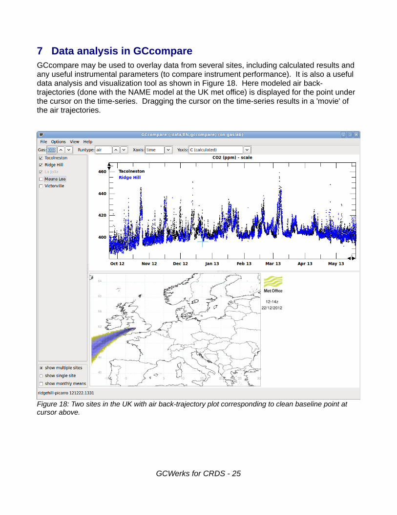
7 Data analysis in GCcompareGCcompare may be used to overlay data from several sites, including calculated results and any useful instrumental parameters (to compare instrument performance). It is also a useful data analysis and visualization tool as shown in Figure 18. Here modeled air back-trajectories (done with the NAME model at the UK met office) is displayed for the point under the cursor on the time-series. Dragging the cursor on the time-series results in a 'movie' of the air trajectories.


Figure 18: Two sites in the UK with air back-trajectory plot corresponding to clean baseline point at cursor above.

8 Acquiring data with GCWerksFigure 19 shows the GCWerks instrument control display with a sequence running to acquire data from a Picarro 2401. The real time strip-chart and numerical displays can show any of the CRDS instrument or other sample data (such as inlet pressure, ambient temperature, etc.).

In addition to automated control from the sequence, the valve position can be controlled interactively from the panel.


Figure 19: GCWerks acquiring data from Picarro 2401.

8.1 Sequence file

An example default sequence is shown below. Any number of sequences may be created and scheduled to run at various times. The default sequence simply repeats forever if nothingelse is scheduled. The sequence specifies the run type (air, cal), the inlet port, and the duration of each measurement.


Figure 20: An example default sequence which runs air on port 1 and calibration tanks from ports 2 and 3.

8.2 Configuring Picarro for data acquisition

The instructions and figures below apply generally to the G2000 series Picarro (G2301, 2302,G2401, etc.). These steps enable data acquisition over TCP/IP via the GCWerks CRDS software:

1) Stop analyzer software only. Do not shut down the analyzer, only stop the software.

2) Under the Picarro Setup Tool "Port Manager" tab, set "TCP" for the "Command Interface" as shown in Figure 21, then press "Apply".

3) Under the Picarro Setup Tool "Command Interface" tab, select all the available output data columns as shown in Figure 22, then press "Apply".

4) Either disable the Windows Firewall or enable TCP port 51020.

5) Set user calibration factors of 1000 for species better reported in ppb units (CH4, CO and N2O) as shown in Figure 24. This step increases the number of significant digits acquired over TCP/IP. Since Picarro reports values over TCP/IP to 3 decimal places inppm units, this corresponds to only 1 ppb resolution. By applying user calibration factor 1000, this increases the resolution to 0.001 ppb.

6) Start the analyzer software

After the Picarro software is restarted test that the TCP/IP port is open by using telnet:

telnet picarro_IP_address 51020



Figure 21: Select TCP for "Command Interface" under the "Port Manager" tab and press Apply.


Figure 22: "Command Interface" tab for Picarro G2401. Select all data columns and press Apply.


Figure 23: "Command Interface" tab for Picarro G2301. Select all data columns and press Apply.


Figure 24: Set ppb units for CH4, CO and N2O with user calibration factor 1000. This also increases the number of significant digits acquired over TCP/IP. NOTE: the name of this file varies by Picarro model. For G2301 UserCal_CFADS.ini, for G2401 UserCal_CFKADS.ini.

Documents

GCWerks for CRDS