Hyperboloid Bridge tutorial in Generative Components This is an edited and revised version of a tutorial written as coursework whilst at Liverpool University School of Architecture on Andre Brown, Michael Knight and Martin Winchester’s Advanced CAAD third year module. The text and images refer to an early version of Generative Components v8, therefore the programme set ups maybe slightly different and the images may not be exact to what this version of the tutorial gives you. Having used v8i, which is the latest version – the information here can still be applied. The downloadable .gct file has been composed, tried and tested in v8 XM 8.5.5. If you are new to GC the first thing to understand is the interface.

Figure 1

View 1, the symbolic view, shows the components relationships. The main view, view 2, shows the geometric result and the features you have placed to form it. It shows your physical model and you can drag and move around the features within in it, altering the model. You can pan around the model and visualise the design. The Transaction File (TF) is the generative components panel in which you define and alter variables within the model. The system of boxes in the middle is the main plane system. The plane with the yellow box is the active plane. These windows will not be quite arranged as seen here

but like any window, they can be moved around and altered to preference but it is suggested you can see all the windows at the same time. (Figure 1) Save the TF (TF stands for transaction file), in the form of a .gct file, this can be done by clicking File, Save on the tool bar of the TF. This saves the instruction that is held within the TF, not the geometry. When you re-open the file, the screen will appear blank, but do not worry all the information is held within the TF. When it is opened a list with black dots appears under the title ‘transaction’, clicking one of these will turn it green and you can choose the stage of the instruction to jump to. Each transaction can be expanded to see what is occurring and also suppressed. These steps can be played through by using the standard forward and backward buttons. This is a key feature within parametric design, where the model does not need to be re-drawn to see the different effects of altering a variable. To skip to this at any point within design, click on the transaction file tab in the bottom left of the TF. (Figure 2)

Figure 2 : Highlighting file tab, stages saved within transaction file and the

transactions tab

If you save after every step or major part of the build up, a new graph user change will exist and if you name it you can quickly refer to, and alter a specific transaction, suppress a transaction, add, delete or move a transaction also.

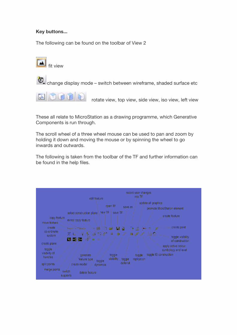
Key buttons... The following can be found on the toolbar of View 2

fit view

change display mode – switch between wireframe, shaded surface etc

rotate view, top view, side view, iso view, left view These all relate to MicroStation as a drawing programme, which Generative Components is run through. The scroll wheel of a three wheel mouse can be used to pan and zoom by holding it down and moving the mouse or by spinning the wheel to go inwards and outwards. The following is taken from the toolbar of the TF and further information can be found in the help files.

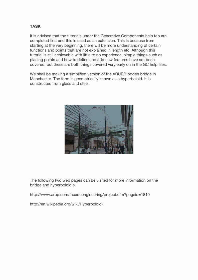
TASK It is advised that the tutorials under the Generative Components help tab are completed first and this is used as an extension. This is because from starting at the very beginning, there will be more understanding of certain functions and points that are not explained in length etc. Although this tutorial is still achievable with little to no experience, simple things such as placing points and how to define and add new features have not been covered, but these are both things covered very early on in the GC help files. We shall be making a simplified version of the ARUP/Hodden bridge in Manchester. The form is geometrically known as a hyperboloid. It is constructed from glass and steel.

The following two web pages can be visited for more information on the bridge and hyperboloid's. http://www.arup.com/facadeengineering/project.cfm?pageid=1810 http://en.wikipedia.org/wiki/Hyperboloid).

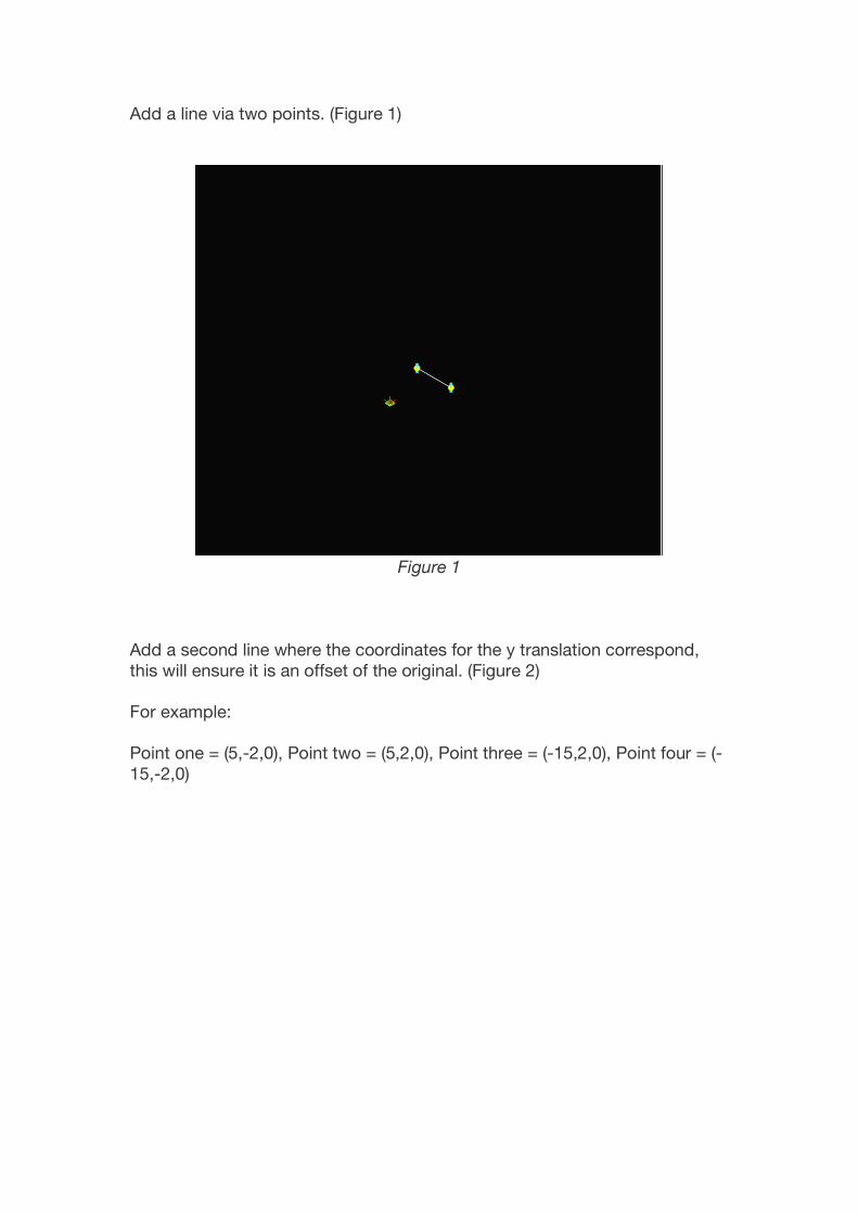
Add a line via two points. (Figure 1)

Figure 1

Add a second line where the coordinates for the y translation correspond, this will ensure it is an offset of the original. (Figure 2) For example: Point one = (5,-2,0), Point two = (5,2,0), Point three = (-15,2,0), Point four = (-15,-2,0)

Figure 2

Apply coordinate systems01 and 02 on the lines, with T of 0.5 and basecs.z direction, using ByParameterAlongCurve as a definition.

Figure 3

Place tangent lines from coordinate system. Line, ByStartPointDirectionLength, Coordinatesystem01 as start point, direction is

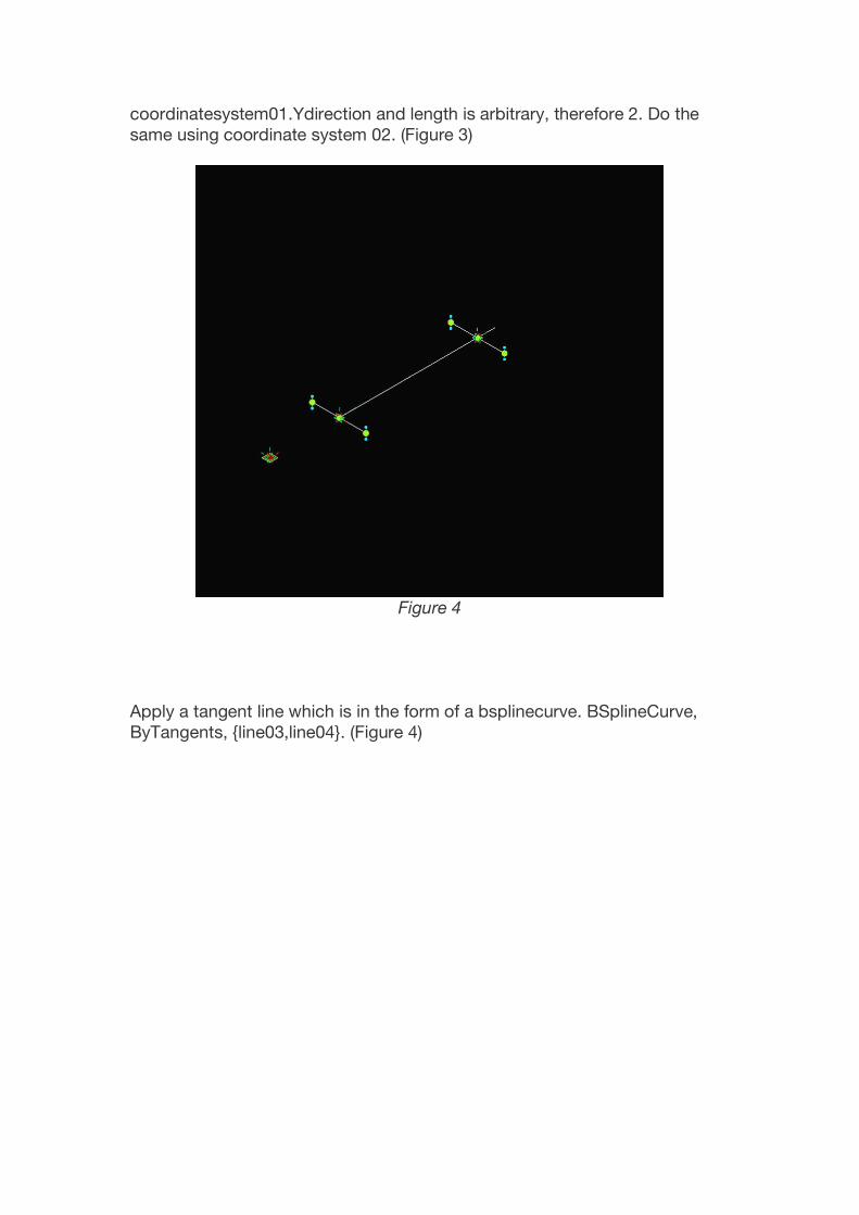
coordinatesystem01.Ydirection and length is arbitrary, therefore 2. Do the same using coordinate system 02. (Figure 3)

Figure 4

Apply a tangent line which is in the form of a bsplinecurve. BSplineCurve, ByTangents, {line03,line04}. (Figure 4)

Figure 5

Apply points along the curve, which we will user as centre points for the hoops. Point, ByDistanceAlongCurve, select curve and then apply series of points eg. If the line is 20 long then Series{0,4,8,12,16,20}. Note : In the gct file I originally placed points every 2, not 4. This is edited later on in the process to use 0,4,8,12,16,20. (Figure 5)

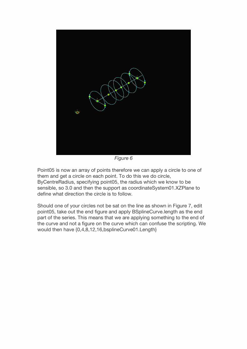
Figure 6

Point05 is now an array of points therefore we can apply a circle to one of them and get a circle on each point. To do this we do circle, ByCentreRadius, specifying point05, the radius which we know to be sensible, so 3.0 and then the support as coordinateSystem01.XZPlane to define what direction the circle is to follow. Should one of your circles not be sat on the line as shown in Figure 7, edit point05, take out the end figure and apply BSplineCurve.length as the end part of the series. This means that we are applying something to the end of the curve and not a figure on the curve which can confuse the scripting. We would then have {0,4,8,12,16,bsplineCurve01.Length}

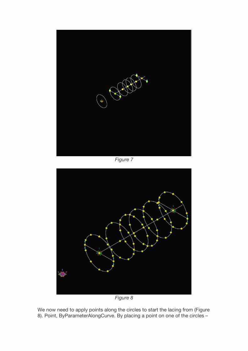
Figure 7

Figure 8

We now need to apply points along the circles to start the lacing from (Figure 8). Point, ByParameterAlongCurve. By placing a point on one of the circles –

which exist as an array, we shall see the point on every circle. If we make the point a series, that series will exist on all the circles. So if we choose circle01 as the curve and then define T as ‘Series(0.0,1.0,0.1)’ we will get points at every 0.1 increment from start to finish. We then need to hit the ‘Toggle Replication Style’ button on the TF to apply this, this maximises the possible replication from our inputs. Next we apply the first set of lacing, which will join on circle[1] to circle[2] from point06[1][3] to point06[2][4] and so on, where the circle index will increase by one every time, as will the point indices, apart from when joining then end hoops. This can be seen in Figure 9.

Figure 9

This is done by Line, ByLacingFromPointGrid and define point06 without brackets and index references. The position index should be 0 and the lacing method should be LacingOption.PositionIndex. We then need the lacing to work in the opposite ‘direction’, so that it would go from point06[1][3] to point06[2][2] and then point06[3][1] and so on. To do this we do the same but input the optional position index as 10. This figure tells the script to do the opposite. (Figure 10)

Figure 10

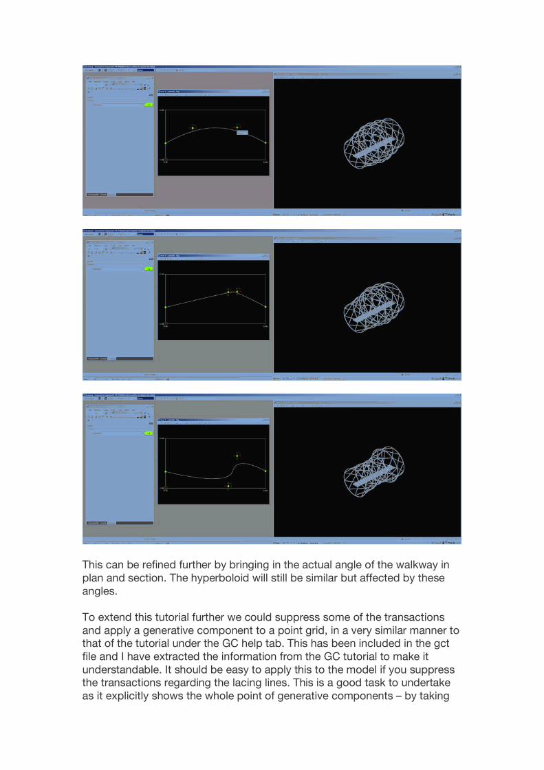
We now apply what is called a law curve, which will allow us to control the form overall/make it interactive, and will be controlled by points in a graph, linked to the radii of the inner hoops, via ‘dependent variables’. First, we require a new control space in which to place a graph, which can then be linked. So to do this we specify a new coordinate system. Coordinate System, AtModelOrigin and type “control2”, including the speech marks. A new window with the new coordinate system will appear. Within this we can now apply the Law Curve Frame.

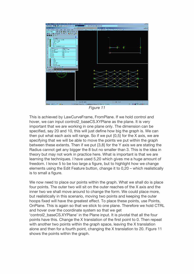
Figure 11

This is achieved by LawCurveFrame, FromPlane. If we hold control and hover, we can input control2_baseCS.XYPlane as the plane. It is very important that we are working in one plane only. The dimension can be specified, say 20 and 10, this will just define how big the graph is. We can then put what each axis will range. So if we put {0,5} for the X axis, we are specifying that we will be able to move the points we put within the graph between these extents. Then if we put {3,8} for the Y axis we are stating the Radius cannot get any bigger the 8 but no smaller than 3. This is the idea in theory but may not work in practice here. What is important is that we are learning the techniques. I have used 5,20 which gives me a huge amount of freedom. I know 5 to be too large a figure, but to highlight how we change elements using the Edit Feature button, change it to 0,20 – which realistically is to small a figure. We now need to place our points within the graph. What we shall do is place four points. The outer two will sit on the outer reaches of the X axis and the inner two we shall move around to change the form. We could place more, but realistically in this scenario, moving two points and keeping the outer hoops fixed will have the greatest effect. To place these points, use Points, OnPlane. This is again so that we stick to one plane. Therefore we hold CTRL and hover over the coordinate system so that we get ‘control2_baseCS.XYPlane’ in the Plane input. It is pivotal that all the four points have this. Change the X translation of the first point to 0. Then repeat with another two points within the graph space, leaving the X translation alone and then for a fourth point, changing the X translation to 20. Figure 11 shows the points within the graph.

We then need to apply the actual curve which is done by LawCurve, ByControlPoints. First we specify the LawCurveFrame which can be done by hold CTRL and hovering over the frame, giving ‘lawCurveFrame01’. Next input the points as Controlpoints, as a list, therefore {point07,point08,point09,point10}, and make sure they are in the order in which they exist left to right. If we make the CurveControl input box active we are immediately faced with an options list. Select ByPoles, although in this case it would have little affect which way the curve was controlled. Put the order as 3. This is for the same reason as before in that 2 would be a polyline and 4 is the maximal control points. For the IndependentVariables, input ‘Series(0,5,1)’, which is defining a series of variables. We will fix the curve to the circle at a later point.

Figure 12

Something like Figure 12 will now exist. We now need to give the bridge some substance and so we will apply cones to make the form look like it is made from steel tubing. To do this we apply a cone via, Cone, ByLine. Select one of the sets of lacing, eg line06. Specify a start and end radius, 0.1 will look sensible. Then repeat this to the other set of lacing. Figure 13, show both sets on cones applied.

Figure 13

We also need to do this to the hoops. We do this once and it will apply it to all of them. We will have to do this as a BSplineSurface. Therefore, BSplineSurface, SweepCircleAlongCurve. This will give us the same effect as a cone did in the straight lines. Select circle01 as the curve, making sure the indices are removed. For diameter put 0.2 and we put 0.1 as a radius for the cones. (Figure 14)

Figure 14

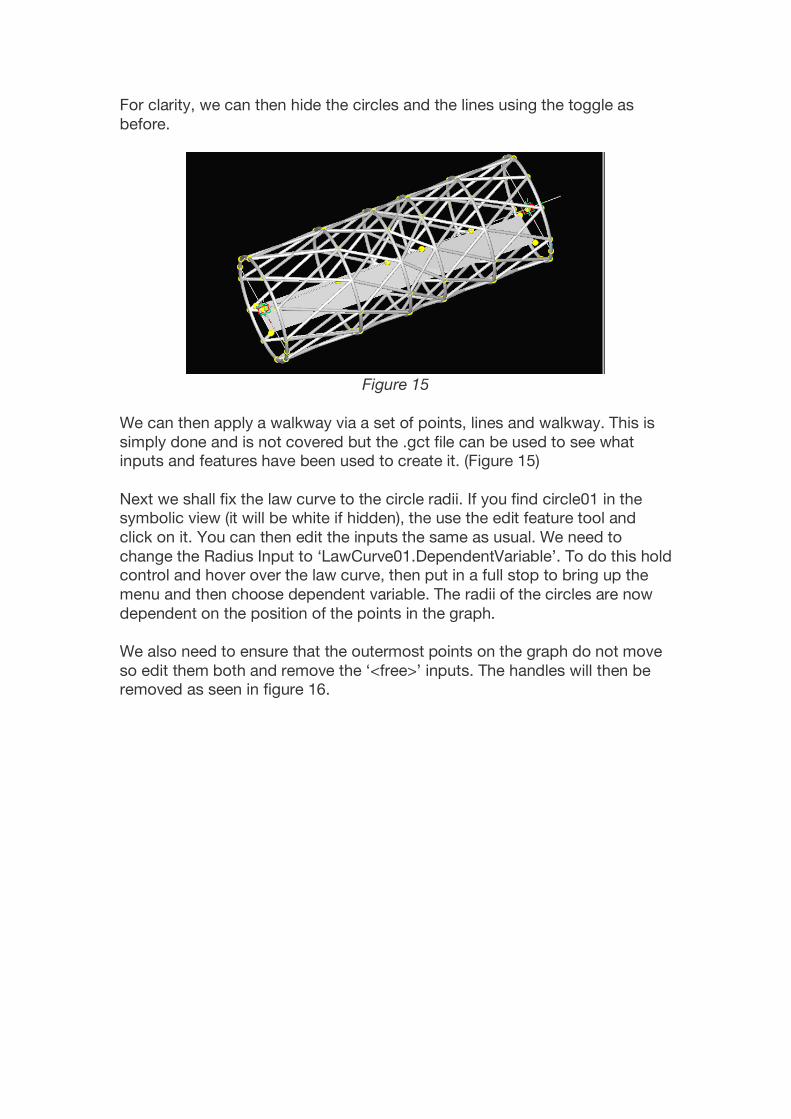
For clarity, we can then hide the circles and the lines using the toggle as before.

Figure 15

We can then apply a walkway via a set of points, lines and walkway. This is simply done and is not covered but the .gct file can be used to see what inputs and features have been used to create it. (Figure 15) Next we shall fix the law curve to the circle radii. If you find circle01 in the symbolic view (it will be white if hidden), the use the edit feature tool and click on it. You can then edit the inputs the same as usual. We need to change the Radius Input to ‘LawCurve01.DependentVariable’. To do this hold control and hover over the law curve, then put in a full stop to bring up the menu and then choose dependent variable. The radii of the circles are now dependent on the position of the points in the graph. We also need to ensure that the outermost points on the graph do not move so edit them both and remove the ‘<free>’ inputs. The handles will then be removed as seen in figure 16.

Figure 16

You can also see that I’ve moved the points and the form has changed.

Figure 17

We can use the toggles to hide what is not necessary visually and by moving the points we can get something near to the bridge in Manchester, shown in Figure 17. By moving the points we can get some of the following results…

This can be refined further by bringing in the actual angle of the walkway in plan and section. The hyperboloid will still be similar but affected by these angles. To extend this tutorial further we could suppress some of the transactions and apply a generative component to a point grid, in a very similar manner to that of the tutorial under the GC help tab. This has been included in the gct file and I have extracted the information from the GC tutorial to make it understandable. It should be easy to apply this to the model if you suppress the transactions regarding the lacing lines. This is a good task to undertake as it explicitly shows the whole point of generative components – by taking

one simple feature, applying it to a system and if necessary getting a completely different result and form for each iteration of it, even though you have only drawn one. The .dll file is the generative component which can be loaded via Tools_Manage Loaded Assemblies_Select Pre-complied Assembly File (*.dll) should it be needed. Some of these instructions may appear brief in what we do in places. This is because they are not necessary to know in the early stage, but if this is carried out with GC’s tutorials, the key techniques should now be picked up. Information for applying a simple generative component (taken from the Bentley GC help files which I then re-wrote for coursework on the Advanced CAAD course at the University of Liverpool Architecture School) : “Using these points we need to form the actual polygon grid. This is done by Polygon, ByPointGrid. Remove the indexes and brackets leaving just point05. The program then knows just to use all the point05’s to from a grid. (This would be done with point06 in the hyperboloid task) We will now make a crossbar panel which gives us a more elegant aesthetic and can also be manipulated by the original four points. This will be created away from the model and then applied. Place four points as shown in Figure 12.

Figure 12 – Placing crossbar points

Make a polygon from these points via Polygon, ByVertices. The vertices will be each of the four points. The polygon will be formed and hide the points as in Figure 13.

Figure 13 – Polygon formed

Next, we create the diagonals, Line, Bypoints, where start point is ‘polygon02.vertices[0]’ and end point is ‘polygon02.vertices[2]’ and then via create copy use [1] and [3] for the other. (Figure 14)

Figure 14 – Diagonals applied

A ‘cone’ is then applied to each diagonal, which effectively acts a tube in this scenario. We do this by Cone, ByLine. The radius needs to be proportional to the diagonal length and not a fixed figure so that the model works and can be manipulated. Line should ‘line04’ and Startradius should be ‘line04.Length/25.0’. Repeat this for line05 using line05 where necessary. 25.0 is editable and arbitrary. (In the hyperboloid example, simply 0.1 as a radius will suffice). The applied cones can be seen in Figure 15.

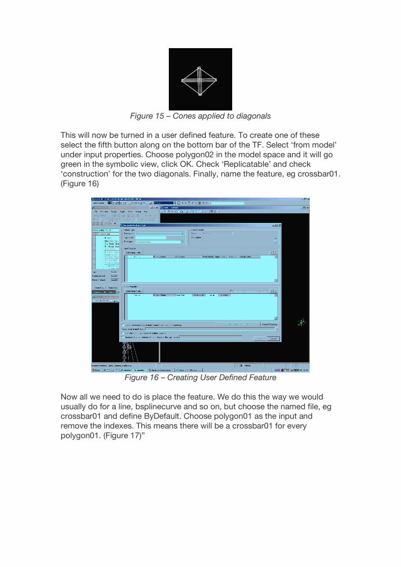
Figure 15 – Cones applied to diagonals

This will now be turned in a user defined feature. To create one of these select the fifth button along on the bottom bar of the TF. Select ‘from model’ under input properties. Choose polygon02 in the model space and it will go green in the symbolic view, click OK. Check ‘Replicatable’ and check ‘construction’ for the two diagonals. Finally, name the feature, eg crossbar01. (Figure 16)

Figure 16 – Creating User Defined Feature

Now all we need to do is place the feature. We do this the way we would usually do for a line, bsplinecurve and so on, but choose the named file, eg crossbar01 and define ByDefault. Choose polygon01 as the input and remove the indexes. This means there will be a crossbar01 for every polygon01. (Figure 17)”

Figure 17 – crossbar01 applied.

If this is applied to the hyperboloid task and all the unnecessary lines, points and surfaces are hidden, then the results should look exactly the same and with the lacing, BUT one generative component has been applied and altered numerous times across the form and more information could be taken from this in terms of sizing etc. through excel and in theory for manufacture. Excel inputs/outputs and fabrication planning are further tools which make GC very worthwhile. These, along with all other features etc can be explored at any time via the ‘Example’ button on the TF. This will not affect your modelling or file, as it just opens up as a second symbolic and modelling view which can be closed, and it will show how to use the definition and what it requires. Questions please…