Embed Size (px)
Citation preview
Gaussian Mixture Models
David Rosenberg, Brett Bernstein
New York University
April 26, 2017
David Rosenberg, Brett Bernstein (New York University)DS-GA 1003 April 26, 2017 1 / 42

Intro Question
Intro Question
David Rosenberg, Brett Bernstein (New York University)DS-GA 1003 April 26, 2017 2 / 42
Intro Question
Intro Question
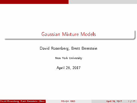
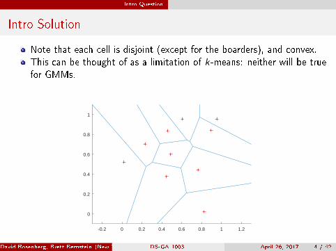
Suppose we begin with a dataset D= {x1, . . . ,xn}⊆ R2 and we runk-means (or k-means++) to obtain k cluster centers. Below we havedrawn the cluster centers. If we are given a new x ∈ R2, we can assign it alabel based on which cluster center is closest. What regions of the planebelow correspond to each possible labeling?
-0.2 0 0.2 0.4 0.6 0.8 1 1.2
0
0.2
0.4
0.6
0.8
1
David Rosenberg, Brett Bernstein (New York University)DS-GA 1003 April 26, 2017 3 / 42
Intro Question
Intro Solution
Note that each cell is disjoint (except for the boarders), and convex.This can be thought of as a limitation of k-means: neither will be truefor GMMs.
-0.2 0 0.2 0.4 0.6 0.8 1 1.2
0
0.2
0.4
0.6
0.8
1
David Rosenberg, Brett Bernstein (New York University)DS-GA 1003 April 26, 2017 4 / 42

Gaussian Mixture Models
Gaussian Mixture Models
David Rosenberg, Brett Bernstein (New York University)DS-GA 1003 April 26, 2017 5 / 42
Gaussian Mixture Models
Yesterday's Intro Question
Consider the following probability model for generating data.
1 Roll a weighted k-sided die to choose a label z ∈ {1, . . . ,k}. Let πdenote the PMF for the die.
2 Draw x ∈ Rd randomly from the multivariate normal distributionN(µz ,Σz).
Solve the following questions.
1 What is the joint distribution of x ,z given π and the µz ,Σz values?
2 Suppose you were given the dataset D= {(x1,z1), . . . ,(xn,zn)}. Howwould you estimate the die weightings, and the µz ,Σz values?
3 How would you determine the label for a new datapoint x?
David Rosenberg, Brett Bernstein (New York University)DS-GA 1003 April 26, 2017 6 / 42
Gaussian Mixture Models
Yesterday's Intro Solution
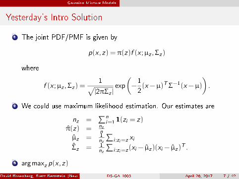
1 The joint PDF/PMF is given by
p(x ,z) = π(z)f (x ;µz ,Σz)
where
f (x ;µz ,Σz) =1√
|2πΣz |exp
(−1
2(x −µ)TΣ−1(x −µ)
).
2 We could use maximum likelihood estimation. Our estimates are
nz =∑n
i=11(zi = z)π̂(z) = nz
nµ̂z = 1
nz
∑i :zi=z xi
Σ̂z = 1nz
∑i :zi=z(xi − µ̂z)(xi − µ̂z)
T .
3 argmaxz p(x ,z)
David Rosenberg, Brett Bernstein (New York University)DS-GA 1003 April 26, 2017 7 / 42
Gaussian Mixture Models
Probabilistic Model for Clustering
Let's consider a generative model for the data.
Suppose
1 There are k clusters.2 We have a probability density for each cluster.
Generate a point as follows
1 Choose a random cluster z ∈ {1,2, . . . ,k}.2 Choose a point from the distribution for cluster Z .
The clustering algorithm is then:1 Use training data to �t the parameters of the generative model.2 For each point, choose the cluster with the highest likelihood based on
model.
David Rosenberg, Brett Bernstein (New York University)DS-GA 1003 April 26, 2017 8 / 42
Gaussian Mixture Models
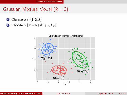
Gaussian Mixture Model (k = 3)
1 Choose z ∈ {1,2,3}
2 Choose x | z ∼ N (X | µz ,Σz).
David Rosenberg, Brett Bernstein (New York University)DS-GA 1003 April 26, 2017 9 / 42
Gaussian Mixture Models
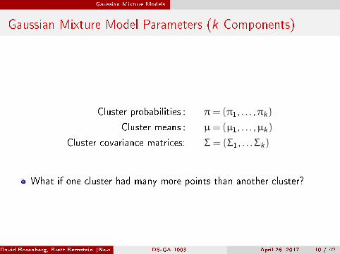
Gaussian Mixture Model Parameters (k Components)
Cluster probabilities : π= (π1, . . . ,πk)
Cluster means : µ= (µ1, . . . ,µk)
Cluster covariance matrices: Σ= (Σ1, . . .Σk)
What if one cluster had many more points than another cluster?
David Rosenberg, Brett Bernstein (New York University)DS-GA 1003 April 26, 2017 10 / 42
Gaussian Mixture Models
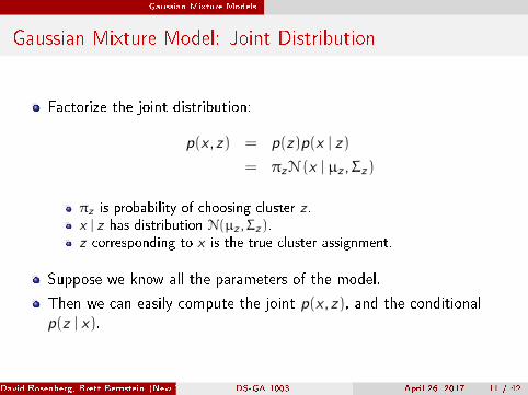
Gaussian Mixture Model: Joint Distribution
Factorize the joint distribution:
p(x ,z) = p(z)p(x | z)
= πzN (x | µz ,Σz)
πz is probability of choosing cluster z .x | z has distribution N(µz ,Σz).z corresponding to x is the true cluster assignment.
Suppose we know all the parameters of the model.
Then we can easily compute the joint p(x ,z), and the conditionalp(z | x).
David Rosenberg, Brett Bernstein (New York University)DS-GA 1003 April 26, 2017 11 / 42
Gaussian Mixture Models
Latent Variable Model
We observe x .
In the intro problem we had labeled data, but here we don't observe z ,the cluster assignment.
Cluster assignment z is called a hidden variable or latent variable.
De�nition
A latent variable model is a probability model for which certain variablesare never observed.
e.g. The Gaussian mixture model is a latent variable model.
David Rosenberg, Brett Bernstein (New York University)DS-GA 1003 April 26, 2017 12 / 42
Gaussian Mixture Models
The GMM �Inference� Problem
We observe x . We want to know z .
The conditional distribution of the cluster z given x is
p(z | x) = p(x ,z)/p(x)
The conditional distribution is a soft assignment to clusters.
A hard assignment is
z∗ = argmaxz∈{1,...,k}
p(z | x).
So if we have the model, clustering is trivial.
David Rosenberg, Brett Bernstein (New York University)DS-GA 1003 April 26, 2017 13 / 42

Mixture Models
Mixture Models
David Rosenberg, Brett Bernstein (New York University)DS-GA 1003 April 26, 2017 14 / 42
Mixture Models
Gaussian Mixture Model: Marginal Distribution
The marginal distribution for a single observation x is
p(x) =
k∑z=1
p(x ,z)
=
k∑z=1
πzN (x | µz ,Σz)
Note that p(x) is a convex combination of probability densities.
This is a common form for a probability model...
David Rosenberg, Brett Bernstein (New York University)DS-GA 1003 April 26, 2017 15 / 42
Mixture Models
Mixture Distributions (or Mixture Models)
De�nition
A probability density p(x) represents a mixture distribution or mixture
model, if we can write it as a convex combination of probabilitydensities. That is,
p(x) =k∑
i=1
wipi (x),
where wi > 0,∑k
i=1wi = 1, and each pi is a probability density.
In our Gaussian mixture model, x has a mixture distribution.
More constructively, let S be a set of probability distributions:
1 Choose a distribution randomly from S .2 Sample x from the chosen distribution.
Then x has a mixture distribution.
David Rosenberg, Brett Bernstein (New York University)DS-GA 1003 April 26, 2017 16 / 42
Learning in Gaussian Mixture Models
Learning in Gaussian Mixture Models
David Rosenberg, Brett Bernstein (New York University)DS-GA 1003 April 26, 2017 17 / 42
Learning in Gaussian Mixture Models
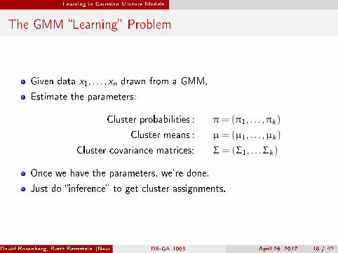
The GMM �Learning� Problem
Given data x1, . . . ,xn drawn from a GMM,
Estimate the parameters:
Cluster probabilities : π= (π1, . . . ,πk)
Cluster means : µ= (µ1, . . . ,µk)
Cluster covariance matrices: Σ= (Σ1, . . .Σk)
Once we have the parameters, we're done.
Just do �inference� to get cluster assignments.
David Rosenberg, Brett Bernstein (New York University)DS-GA 1003 April 26, 2017 18 / 42
Learning in Gaussian Mixture Models
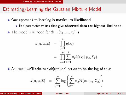
Estimating/Learning the Gaussian Mixture Model
One approach to learning is maximum likelihood
�nd parameter values that give observed data the highest likelihood.
The model likelihood for D= {x1, . . . ,xn} is
L(π,µ,Σ) =
n∏i=1
p(xi )
=
n∏i=1
k∑z=1
πzN (xi | µz ,Σz) .
As usual, we'll take our objective function to be the log of this:
J(π,µ,Σ) =
n∑i=1
log
{k∑
z=1
πzN (xi | µz ,Σz)
}
David Rosenberg, Brett Bernstein (New York University)DS-GA 1003 April 26, 2017 19 / 42
Learning in Gaussian Mixture Models
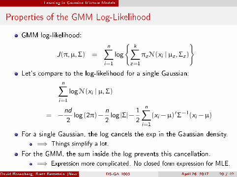
Properties of the GMM Log-Likelihood
GMM log-likelihood:
J(π,µ,Σ) =
n∑i=1
log
{k∑
z=1
πzN (xi | µz ,Σz)
}Let's compare to the log-likelihood for a single Gaussian:
n∑i=1
logN (xi | µ,Σ)
= −nd
2log (2π)−
n
2log |Σ|−
1
2
n∑i=1
(xi −µ)′Σ−1(xi −µ)
For a single Gaussian, the log cancels the exp in the Gaussian density.
=⇒ Things simplify a lot.
For the GMM, the sum inside the log prevents this cancellation.
=⇒ Expression more complicated. No closed form expression for MLE.
David Rosenberg, Brett Bernstein (New York University)DS-GA 1003 April 26, 2017 20 / 42

Issues with MLE for GMM
Issues with MLE for GMM
David Rosenberg, Brett Bernstein (New York University)DS-GA 1003 April 26, 2017 21 / 42
Issues with MLE for GMM
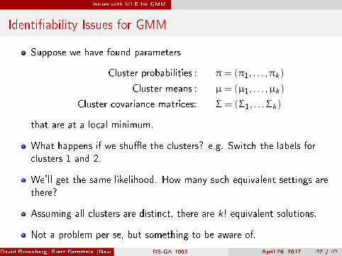
Identi�ability Issues for GMM
Suppose we have found parameters
Cluster probabilities : π= (π1, . . . ,πk)
Cluster means : µ= (µ1, . . . ,µk)
Cluster covariance matrices: Σ= (Σ1, . . .Σk)
that are at a local minimum.
What happens if we shu�e the clusters? e.g. Switch the labels forclusters 1 and 2.
We'll get the same likelihood. How many such equivalent settings arethere?
Assuming all clusters are distinct, there are k! equivalent solutions.
Not a problem per se, but something to be aware of.
David Rosenberg, Brett Bernstein (New York University)DS-GA 1003 April 26, 2017 22 / 42
Issues with MLE for GMM
Singularities for GMM
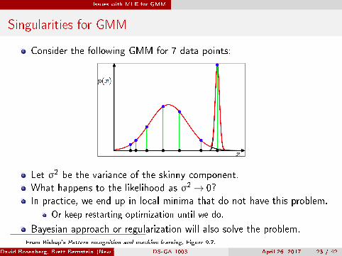
Consider the following GMM for 7 data points:
Let σ2 be the variance of the skinny component.
What happens to the likelihood as σ2→ 0?
In practice, we end up in local minima that do not have this problem.
Or keep restarting optimization until we do.
Bayesian approach or regularization will also solve the problem.From Bishop's Pattern recognition and machine learning, Figure 9.7.
David Rosenberg, Brett Bernstein (New York University)DS-GA 1003 April 26, 2017 23 / 42
Issues with MLE for GMM
Gradient Descent / SGD for GMM
What about running gradient descent or SGD on
J(π,µ,Σ) = −
n∑i=1
log
{k∑
z=1
πzN (xi | µz ,Σz)
}?
Can be done � but need to be clever about it.
Each matrix Σ1, . . . ,Σk has to be positive semide�nite.
How to maintain that constraint?
Rewrite Σi =MiMTi , where Mi is an unconstrained matrix.
Then Σi is positive semide�nite.
David Rosenberg, Brett Bernstein (New York University)DS-GA 1003 April 26, 2017 24 / 42

The EM Algorithm for GMM
The EM Algorithm for GMM
David Rosenberg, Brett Bernstein (New York University)DS-GA 1003 April 26, 2017 25 / 42
The EM Algorithm for GMM
MLE for GMM
From yesterday's intro questions, we know that we can solve the MLEproblem if the cluster assignments zi are known
nz =
n∑i=1
1(zi = z)
π̂(z) =nzn
µ̂z =1
nz
∑i :zi=z
xi
Σ̂z =1
nz
∑i :zi=z
(xi − µ̂z)(xi − µ̂z)T .
In the EM algorithm we will modify the equations to handle ourevolving soft assignments, which we will call responsibilities.
David Rosenberg, Brett Bernstein (New York University)DS-GA 1003 April 26, 2017 26 / 42
The EM Algorithm for GMM
Cluster Responsibilities: Some New Notation
Denote the probability that observed value xi comes from cluster j by
γji = P(Z = j | X = xi ) .
The responsibility that cluster j takes for observation xi .
Computationally,
γji = P(Z = j | X = xi ) .
= p (Z = j ,X = xi )/p(x)
=πjN (xi | µj ,Σj)∑k
c=1πcN (xi | µc ,Σc)
The vector(γ1i , . . . ,γ
ki
)is exactly the soft assignment for xi .
Let nc =∑n
i=1γci be the �number� of points soft assigned to cluster
c .
David Rosenberg, Brett Bernstein (New York University)DS-GA 1003 April 26, 2017 27 / 42
The EM Algorithm for GMM
EM Algorithm for GMM: Overview
If we know π and µj ,Σj for all j then we can easily �nd
γji = P(Z = j | X = xi ).
If we know the (soft) assignments, we can easily �nd estimates for π,µj ,Σj for all j .
Repeatedly alternate the previous 2 steps.
David Rosenberg, Brett Bernstein (New York University)DS-GA 1003 April 26, 2017 28 / 42
The EM Algorithm for GMM
EM Algorithm for GMM: Overview
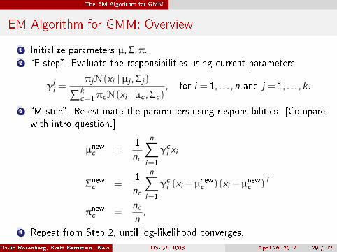
1 Initialize parameters µ,Σ,π.2 �E step�. Evaluate the responsibilities using current parameters:
γji =
πjN (xi | µj ,Σj)∑kc=1πcN (xi | µc ,Σc)
, for i = 1, . . . ,n and j = 1, . . . ,k .
3 �M step�. Re-estimate the parameters using responsibilities. [Comparewith intro question.]
µnewc =1
nc
n∑i=1
γci xi
Σnewc =1
nc
n∑i=1
γci (xi −µnewc )(xi −µ
newc )T
πnewc =ncn,
4 Repeat from Step 2, until log-likelihood converges.
David Rosenberg, Brett Bernstein (New York University)DS-GA 1003 April 26, 2017 29 / 42
The EM Algorithm for GMM
EM for GMM
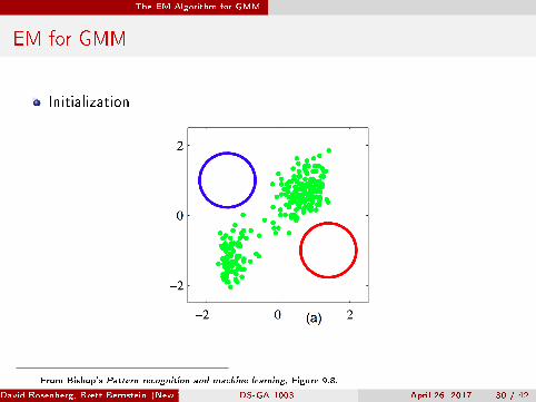
Initialization
From Bishop's Pattern recognition and machine learning, Figure 9.8.
David Rosenberg, Brett Bernstein (New York University)DS-GA 1003 April 26, 2017 30 / 42
The EM Algorithm for GMM
EM for GMM
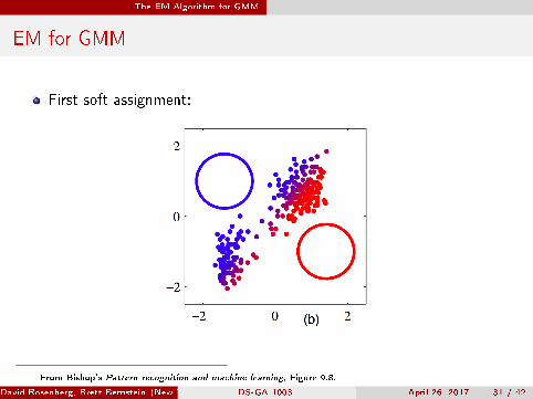
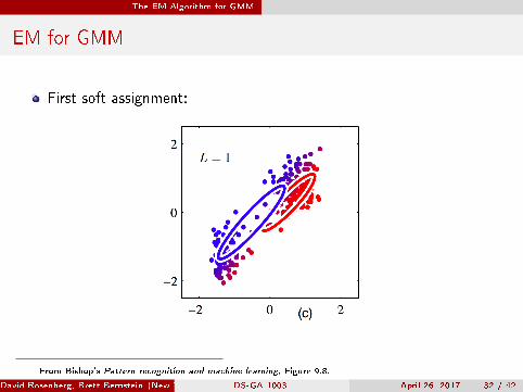
First soft assignment:
From Bishop's Pattern recognition and machine learning, Figure 9.8.
David Rosenberg, Brett Bernstein (New York University)DS-GA 1003 April 26, 2017 31 / 42
The EM Algorithm for GMM
EM for GMM
First soft assignment:
From Bishop's Pattern recognition and machine learning, Figure 9.8.
David Rosenberg, Brett Bernstein (New York University)DS-GA 1003 April 26, 2017 32 / 42
The EM Algorithm for GMM
EM for GMM
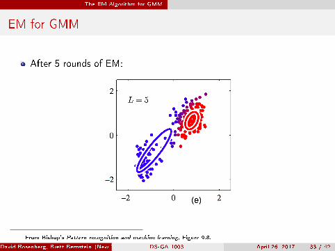
After 5 rounds of EM:
From Bishop's Pattern recognition and machine learning, Figure 9.8.
David Rosenberg, Brett Bernstein (New York University)DS-GA 1003 April 26, 2017 33 / 42
The EM Algorithm for GMM
EM for GMM
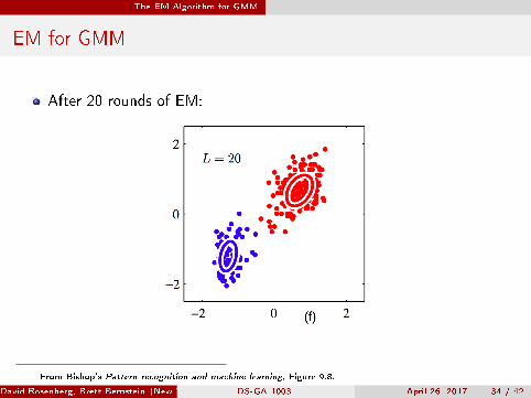
After 20 rounds of EM:
From Bishop's Pattern recognition and machine learning, Figure 9.8.
David Rosenberg, Brett Bernstein (New York University)DS-GA 1003 April 26, 2017 34 / 42
The EM Algorithm for GMM
Relation to K -Means
EM for GMM seems a little like k-means.
In fact, there is a precise correspondence.
First, �x each cluster covariance matrix to be σ2I .
Then the density for each Gausian only depends on distance to themean.
As we take σ2→ 0, the update equations converge to doing k-means.
If you do a quick experiment yourself, you'll �nd
Soft assignments converge to hard assignments.Has to do with the tail behavior (exponential decay) of Gaussian.
Can use k-means++ to initialize parameters of EM algorithm.
David Rosenberg, Brett Bernstein (New York University)DS-GA 1003 April 26, 2017 35 / 42

Math Prerequisites for General EM Algorithm
Math Prerequisites for General EM Algorithm
David Rosenberg, Brett Bernstein (New York University)DS-GA 1003 April 26, 2017 36 / 42
Math Prerequisites for General EM Algorithm
Jensen's Inequality
Which is larger: E[X 2] or E[X ]2?
Must be E[X 2] since Var[X ] = E[X 2]−E[X ]2 > 0.
More general result is true:
Theorem
Jensen's Inequality If f : R→ R is convex and X is a random variable then
E[f (X )]> f (E[X ]). If f is strictly convex then we have equality i�
X = E[X ] with probability 1 (i.e., X is constant).
David Rosenberg, Brett Bernstein (New York University)DS-GA 1003 April 26, 2017 37 / 42
Math Prerequisites for General EM Algorithm
Jensen's Inequality
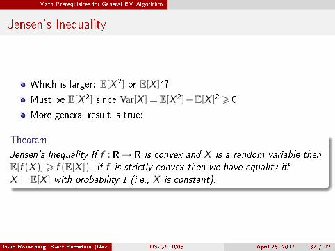
Which is larger: E[X 2] or E[X ]2?
Must be E[X 2] since Var[X ] = E[X 2]−E[X ]2 > 0.
More general result is true:
Theorem
Jensen's Inequality If f : R→ R is convex and X is a random variable then
E[f (X )]> f (E[X ]). If f is strictly convex then we have equality i�
X = E[X ] with probability 1 (i.e., X is constant).
David Rosenberg, Brett Bernstein (New York University)DS-GA 1003 April 26, 2017 37 / 42
Math Prerequisites for General EM Algorithm
Proof of Jensen
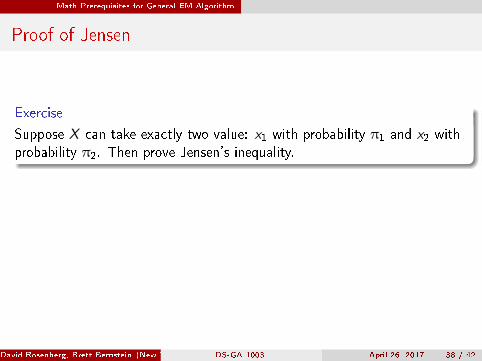
Exercise
Suppose X can take exactly two value: x1 with probability π1 and x2 withprobability π2. Then prove Jensen's inequality.
Let's compute E[f (X )]:
E[f (X )] = π1f (x1)+π2f (x2)6 f (π1x1+π2x2) = f (E[X ]).
For the general proof, what do we know is true about all convexfunctions f : R→ R?
David Rosenberg, Brett Bernstein (New York University)DS-GA 1003 April 26, 2017 38 / 42
Math Prerequisites for General EM Algorithm
Proof of Jensen
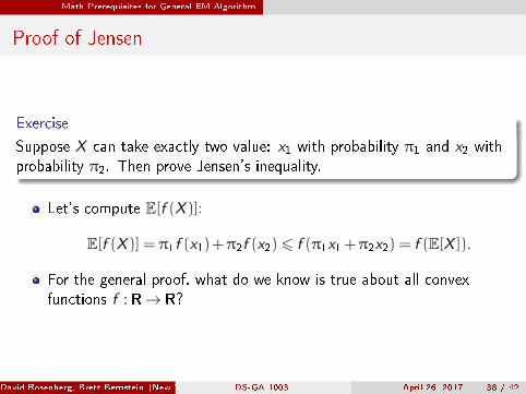
Exercise
Suppose X can take exactly two value: x1 with probability π1 and x2 withprobability π2. Then prove Jensen's inequality.
Let's compute E[f (X )]:
E[f (X )] = π1f (x1)+π2f (x2)6 f (π1x1+π2x2) = f (E[X ]).
For the general proof, what do we know is true about all convexfunctions f : R→ R?
David Rosenberg, Brett Bernstein (New York University)DS-GA 1003 April 26, 2017 38 / 42
Math Prerequisites for General EM Algorithm
Proof of Jensen
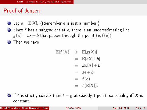
1 Let e = E[X ]. (Remember e is just a number.)
2 Since f has a subgradient at e, there is an underestimating lineg(x) = ax +b that passes through the point (e, f (e)).
3 Then we have
E[f (X )] > E[g(X )]
= E[aX +b]
= aE[X ]+b
= ae+b
= f (e)
= f (E[X ]).
4 If f is strictly convex then f = g at exactly 1 point, so equality i� X isconstant.
David Rosenberg, Brett Bernstein (New York University)DS-GA 1003 April 26, 2017 39 / 42
Math Prerequisites for General EM Algorithm
KL-Divergence
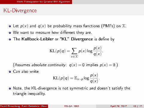
Let p(x) and q(x) be probability mass functions (PMFs) on X.
We want to measure how di�erent they are.
The Kullback-Leibler or �KL� Divergence is de�ne by
KL(p‖q) =∑x∈X
p(x) logp(x)
q(x).
(Assumes absolute continuity : q(x) = 0 implies p(x) = 0.)
Can also write
KL(p‖q) = Ex∼p logp(x)
q(x).
Note, the KL-divergence is not symmetric and doesn't satisfy thetriangle inequality.
David Rosenberg, Brett Bernstein (New York University)DS-GA 1003 April 26, 2017 40 / 42
Math Prerequisites for General EM Algorithm
Gibbs' Inequality
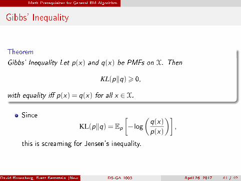
Theorem
Gibbs' Inequality Let p(x) and q(x) be PMFs on X. Then
KL(p‖q)> 0,
with equality i� p(x) = q(x) for all x ∈ X.
Since
KL(p‖q) = Ep
[− log
(q(x)
p(x)
)],
this is screaming for Jensen's inequality.
David Rosenberg, Brett Bernstein (New York University)DS-GA 1003 April 26, 2017 41 / 42
Math Prerequisites for General EM Algorithm
Gibbs' Inequality: Proof
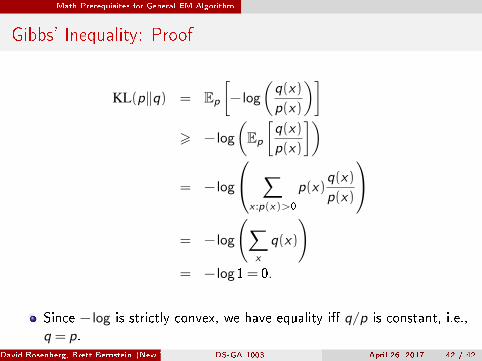
KL(p‖q) = Ep
[− log
(q(x)
p(x)
)]> − log
(Ep
[q(x)
p(x)
])
= − log
∑x :p(x)>0
p(x)q(x)
p(x)
= − log
(∑x
q(x)
)= − log1= 0.
Since − log is strictly convex, we have equality i� q/p is constant, i.e.,q = p.
David Rosenberg, Brett Bernstein (New York University)DS-GA 1003 April 26, 2017 42 / 42