Embed Size (px)
Citation preview
4Gauge Theories and the Standard
Model
In the first chapter, we focused on quantum field theories of free fermions. In order to
construct renormalizable interacting quantum field theories, we must introduce ad-
ditional fields. The requirement of renormalizability imposes two constraints. First,
the terms of the interaction Lagrangian must be no higher than mass dimension-
four. Thus, no (perturbatively) renormalizable interacting theory that consists only
of spin-1/2 fields exists, since the simplest interaction term involving fermions is a
dimension-six four-fermion interaction. Renormalizable interacting theories consist-
ing of scalars, fermions and spin-one bosons can be constructed. The vector bosons
must either be abelian vector fields or non-abelian gauge fields. This exhausts all
possible renormalizable field theories.
The Standard Model is a spontaneously broken non-abelian gauge theory contain-
ing elementary scalars, fermions and spin-one gauge bosons. Typically, one refers
to the spin-0 and spin-1/2 fields (which are either neutral or charged with respect
to the underlying gauge group) as matter fields, whereas the spin-1 gauge bosons
are called gauge fields. In this chapter we review the ingredients for construct-
ing non-abelian (Yang-Mills) gauge theories and their breaking via the dynamics
of self-interacting scalar fields. The Standard Model of fundamental particles and
interactions is then exhibited, and some of its properties are described.
4.1 Abelian Gauge field theory
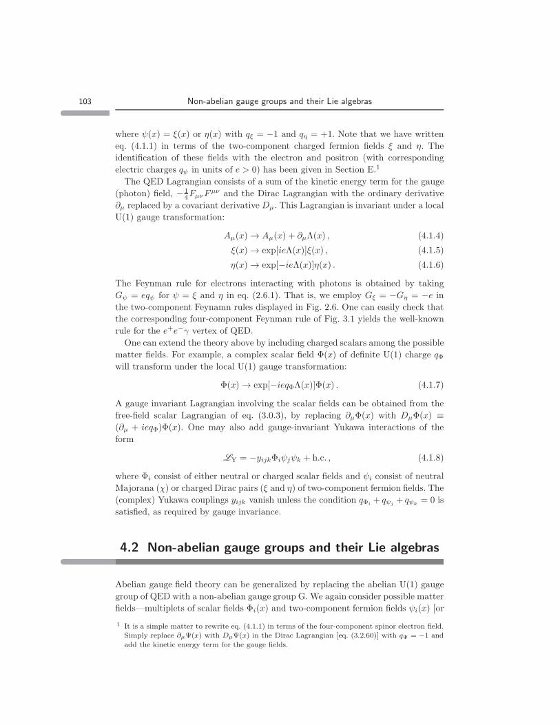
The first (and simplest) known gauge theory is quantum electrodynamics (QED).
This was a very successful theory that described the interactions of electrons,
positrons and photons. The Lagrangian of QED is given by:
L = − 14F
µνFµν + iξ† σµDµξ + iη† σµDµη −m(ξη + ξ† η†) , (4.1.1)
where the electromagnetic field strength tensor Fµν is defined in terms of the gauge
field Aµ as
Fµν ≡ ∂µAν − ∂νAµ , (4.1.2)
and the covariant derivative Dµ is defined as:
Dµψ(x) ≡ (∂µ + ieqψAµ)ψ(x) , (4.1.3)
102
103 Non-abelian gauge groups and their Lie algebras
where ψ(x) = ξ(x) or η(x) with qξ = −1 and qη = +1. Note that we have written
eq. (4.1.1) in terms of the two-component charged fermion fields ξ and η. The
identification of these fields with the electron and positron (with corresponding
electric charges qψ in units of e > 0) has been given in Section E.1
The QED Lagrangian consists of a sum of the kinetic energy term for the gauge
(photon) field, − 14FµνF
µν and the Dirac Lagrangian with the ordinary derivative
∂µ replaced by a covariant derivative Dµ. This Lagrangian is invariant under a local
U(1) gauge transformation:
Aµ(x)→ Aµ(x) + ∂µΛ(x) , (4.1.4)
ξ(x)→ exp[ieΛ(x)]ξ(x) , (4.1.5)
η(x)→ exp[−ieΛ(x)]η(x) . (4.1.6)
The Feynman rule for electrons interacting with photons is obtained by taking
Gψ = eqψ for ψ = ξ and η in eq. (2.6.1). That is, we employ Gξ = −Gη = −e in
the two-component Feynamn rules displayed in Fig. 2.6. One can easily check that
the corresponding four-component Feynman rule of Fig. 3.1 yields the well-known
rule for the e+e−γ vertex of QED.
One can extend the theory above by including charged scalars among the possible
matter fields. For example, a complex scalar field Φ(x) of definite U(1) charge qΦwill transform under the local U(1) gauge transformation:
Φ(x)→ exp[−ieqΦΛ(x)]Φ(x) . (4.1.7)
A gauge invariant Lagrangian involving the scalar fields can be obtained from the
free-field scalar Lagrangian of eq. (3.0.3), by replacing ∂µΦ(x) with DµΦ(x) ≡(∂µ + ieqΦ)Φ(x). One may also add gauge-invariant Yukawa interactions of the
form
LY = −yijkΦiψjψk + h.c. , (4.1.8)
where Φi consist of either neutral or charged scalar fields and ψi consist of neutral
Majorana (χ) or charged Dirac pairs (ξ and η) of two-component fermion fields. The
(complex) Yukawa couplings yijk vanish unless the condition qΦi+ qψj
+ qψk= 0 is
satisfied, as required by gauge invariance.
4.2 Non-abelian gauge groups and their Lie algebras
Abelian gauge field theory can be generalized by replacing the abelian U(1) gauge
group of QED with a non-abelian gauge group G. We again consider possible matter
fields—multiplets of scalar fields Φi(x) and two-component fermion fields ψi(x) [or
1 It is a simple matter to rewrite eq. (4.1.1) in terms of the four-component spinor electron field.Simply replace ∂µΨ(x) with DµΨ(x) in the Dirac Lagrangian [eq. (3.2.60)] with qΨ = −1 and
add the kinetic energy term for the gauge fields.
104 Gauge Theories and the Standard Model
equivalently, four component fermions Ψi(x)] that are either neutral or charged
with respect to G.
The symmetry group G can be expressed in general as a direct product of a finite
number of simple compact Lie groups and U(1). A direct product of simple Lie
groups [i.e., with no U(1) factors] is called a semi-simple Lie group. The list of all
possible simple Lie groups are known and consist of SU(n), SO(n), Sp(n) and five
exceptional groups (G2, F4, E6, E7 and E8). Given some matter field (either scalar
or fermion), which we generically designate by φi(x), the gauge transformation
under which the Lagrangian is invariant, is given by:
φi(x)→ Uij(g)φj(x) , i, j = 1, 2, . . . , d(R) , (4.2.1)
where g is an element of G (that is, g is a specific gauge transformation) and U(g)
is a (possibly reducible) d(R)-dimensional unitary representation R of the group G.
One is always free to redefine the fields via φ(x) → V φ(x), where V is any fixed
unitary matrix (independent of the choice of g). The gauge transformation law for
the redefined φ(x) now has U(g) replaced by V −1U(g)V . If U(g) is a reducible
representation, then it is possible to find a V such that the U(g) for all group
elements g assume a block diagonal form. Otherwise, the representation U(g) is
irredicible. The matter fields of the gauge theory generally form a reducible rep-
resentation, which can subsequently be decomposed into their irreducible pieces.
Irreducible representations imply that the corresponding multiplets transform only
among themselves, and thus we can focus on these pieces separately without loss
of generality.
The local gauge transformation U(g) is also a function of space-time position, xµ.
Explicitly, any group element that is continuously connected to the identity takes
the following form:
U(g(x)) = exp[−igaΛa(x)T a] , (4.2.2)
where there is an implicit sum over the repeated index a = 1, 2, . . . , dG. The T a
are a set of dG linearly independent hermitian matrices2 called generators of the
Lie group, and the corresponding Λa(x) are arbitrary x-dependent functions. The
constants ga (which is analogous to e of the abelian theory) are called the gauge
couplings. There is a separate coupling ga for each simple group or U(1) factor of
the gauge group G. Thus, the generators T a separate out into distinct classes, each
of which is associated with a simple group or one of the U(1) factors contained in
the direct product that defines G. In particular, ga = gb if T a and T b are in the
same class. If G is simple, then ga = g for all a.
Lie group theory teaches us that the number of linearly independent generators,
dG, depends only on the abstract definition of G (and not on the choice of repre-
sentation). Thus, dG is also called the dimension of the Lie group G. Moreover, the
2 The condition of linear independence means that caTa = 0 (implicit sum over a) implies that
ca = 0 for all a.

105 Non-abelian gauge groups and their Lie algebras
commutator of two generators is a linear combination of generators:
[T a, T b] = ifabcT c , (4.2.3)
where the fabc are called the structure constants of the Lie group. In studying the
stucture of gauge field theories, nearly all the information of interest can be ascer-
tained by focusing on infinitesimal gauge transformations. In a given representation
R, one can expand about the d(R)×d(R) identity matrix any matrix representation
of a group element U(g(x)) that is continuously connected to the identity element:
U(g(x)) ≃ Id(R) − igaΛa(x)T a , (4.2.4)
where the T a comprise a d(R)-dimensional representation of the Lie group gener-
ators. Then, the infinitesimal gauge transformation corresponding to eq. (4.2.1) is
given by φi(x)→ φi(x) + δφi(x), where
δφi(x) = −igaΛa(x)(T a)ijφj(x) . (4.2.5)
From the generators T a, one can reconstruct the group elements U(g(x)), so it is
sufficient to focus on the infinitesimal group transformations. The group generators
T a span a real vector space, whose general element is caT a, where the ca are real
numbers.3 One can formally define a “vector product” of any two elements of the
vector space as the commutator of the two vectors. For example, using eq. (4.2.3),
it is clear that the vector product of any two vectors [caT a, dbT b] is a real linear
combination of the generators, which is also an element of the vector space. Con-
sequently, this vector space is also an algebra, called a Lie algebra. Henceforth, the
Lie algebra corresponding to the Lie group G will be designated by g. A Lie algebra
has one additional important property:
[T a, [T b, T c]
]+[T b, [T c, T a]
]+[T c, [T a, T b]
]= 0 . (4.2.6)
This is called the Jacobi identity, and it is clearly satisfied by any three elements
of the Lie algebra.
If the symmetry group G is a direct product of simple Lie group and U(1) factors,
then its Lie algebra g is a direct sum of a finite number of simple Lie algebras and
u(1).4 A direct sum of simple Lie algebras [i.e., with no u(1) factors] is called a semi-
simple Lie algebra. If T a and T b belong to different classes (i.e., different factors of
the direct sum), then [T a, T b] = 0. Equivalently, fabc = 0 if T a, T b and T c do not
all belong to the same class.
In the next section, we will see that the gauge fields transform under the adjoint
representation of the (global) gauge group. The explicit matrix elements of the
3 With the Ta hermitian, we require the ca to be real in order that U(g) be unitary. Then, theTa span a real Lie algebra. Mathematicians consider the elements of the real Lie algebra to beicaTa, with anti-hermitian generators iTa. Note that for real Lie algebras, the representationmatrices for Ta (or iTa) may be complex or quaternionic.
4 The Lie algebra u(1) is equivalent to the vector space of real numbers. The vector product isthe commuatator, which vanishes for any pair of u(1) elements. Thus, u(1) is an abelian Lie
algebra.

106 Gauge Theories and the Standard Model
adjoint representation generators are given by
(T a)bc = −ifabc a, b, c = 1, 2, . . . , dG . (4.2.7)
Thus, the dimension of the adjoint representation matrices coincides with the num-
ber of generators, dG. Hence, we shall often refer to the indices a, b, c as adjoint
indices. For real Lie algebras, the fabc are real numbers. Note that fabc = −facb[as a consequence of eq. (4.2.3)], so that in the adjoint representation the iT a are
real antisymmetric matrices. The representation matrices of the corresponding Lie
group elements [eq. (4.2.2)] are therefore real and orthogonal. Thus, the adjoint
representation provides a real representation of the Lie group and Lie algebra.
The choice of basis vectors (or generators) T a is arbitrary. Moreover, the values
of the structure constants fabc also depend on this choice of basis. Nevertheless,
there is a canonical choice which we now adopt. The generators are chosen such
that:
Tr(T aT b) = TRδab , (4.2.8)
where TR depends on the irreducible representation of the T a. Having chosen this
basis, there is no distinction between upper and lower adjoint indices.5 Moreover,
in this basis the fabc are completely antisymmetric under the interchange of a, b
and c.6 One can show that once TR is chosen for any one non-trivial irreducible
representation R, then the value of TR for any other irreducible representation is
fixed. Corresponding to each simple real (compact) Lie algebra, one can identify
one particular irreducible representation, called the defining representation (some-
times, but less accurately, called the fundamental representation); the most useful
examples are listed in Table 4.1. For the defining (or fundamental) representation
(which is indicated by R = F ), the conventional value for TR is taken to be:
TF = 12 . (4.2.9)
As noted above, the basis choice of eq. (4.2.8) with the normalization convention
given by eq. (4.2.9) determines the value of TR for an arbitrary irreducible repre-
sentation R. The quantity TR/TF is called the index of the representation R.
For the record, we mention two other properties of Lie algebras that will be
useful in this book. First, given any semi-simple Lie algebra g and a corresponding
irreducible representation of anti-hermitian generators iT a, one can always find an
equivalent representation V −1T aV for some unitary matrix V . There exists some
choice of V (not necessarily unique) that maximizes the number of simultaneous
diagonal generators, V −1T aV . This maximal number rG, called the rank of g, is
independent of the choice of representation, and is a property of the abstract Lie
algebra. The ranks of the classical Lie algebras are given in Table 4.1.
Second, a Casimir operator is defined to be an operator that commutes with
5 More generally, in an arbitrary basis, Tr(TaT b) = TRgab, where gab is the Cartan-Killing form
(which can be used to raise and lower adjoint indices).6 By definition, fabc is antisymmetric under the interchange of a and b. But the complete anti-
symmetry under the interchange of all three indices requires eq. (4.2.8) to be satisfied.
107 Non-abelian gauge field theory
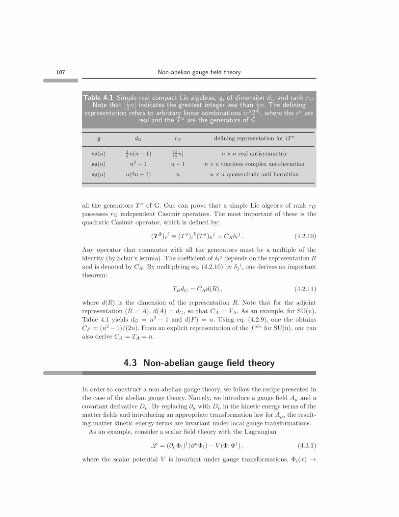
Table 4.1 Simple real compact Lie algebras, g, of dimension dG and rank rG.Note that [1
2n] indicates the greatest integer less than 1
2n. The defining
representation refers to arbitrary linear combinations icaT a, where the ca arereal and the T a are the generators of G.
g dG rG defining representation for iT a
so(n) 12n(n− 1) [ 1
2n] n× n real antisymmetric
su(n) n2 − 1 n− 1 n× n traceless complex anti-hermtian
sp(n) n(2n+ 1) n n× n quaternionic anti-hermitian
all the generators T a of G. One can prove that a simple Lie algebra of rank rGpossesses rG independent Casimir operators. The most important of these is the
quadratic Casimir operator, which is defined by:
(T 2)ij ≡ (T a)i
k(T a)kj = CRδi
j . (4.2.10)
Any operator that commutes with all the generators must be a multiple of the
identity (by Schur’s lemma). The coefficient of δij depends on the representation R
and is denoted by CR. By multiplying eq. (4.2.10) by δji, one derives an important
theorem:
TRdG = CRd(R) , (4.2.11)
where d(R) is the dimension of the representation R. Note that for the adjoint
representation (R = A), d(A) = dG, so that CA = TA. As an example, for SU(n),
Table 4.1 yields dG = n2 − 1 and d(F ) = n. Using eq. (4.2.9), one the obtains
CF = (n2− 1)/(2n). From an explicit representation of the fabc for SU(n), one can
also derive CA = TA = n.
4.3 Non-abelian gauge field theory
In order to construct a non-abelian gauge theory, we follow the recipe presented in
the case of the abelian gauge theory. Namely, we introduce a gauge field Aµ and a
covariant derivative Dµ. By replacing ∂µ with Dµ in the kinetic energy terms of the
matter fields and introducing an appropriate transformation law for Aµ, the result-
ing matter kinetic energy terms are invariant under local gauge transformations.
As an example, consider a scalar field theory with the Lagrangian
L = (∂µΦi)†(∂µΦi)− V (Φ,Φ†) , (4.3.1)
where the scalar potential V is invariant under gauge transformations, Φi(x) →
108 Gauge Theories and the Standard Model
Uij(g)Φj(x); that is,
V (UΦ, (UΦ)†) = V (Φ,Φ†) . (4.3.2)
Although L is invariant under global gauge transformations, the kinetic energy
term is not invariant under local gauge transformations due to the presence of
the derivative. In particular, under local gauge transformations ∂µΦ → ∂µ(UΦ) =
U∂µΦ+(∂µU)Φ. We therefore introduce the covariant derivative acting on a matter
field that transforms according to some representation R of the symmetry group
G:
(Dµ)ij = δi
j∂µ + igaAaµ(x)(T a)i
j , a = 1, 2, . . . , dG , (4.3.3)
where the flavor indices i, j = 1, 2, . . . , d(R). If the symmetry group is simple, then
ga = g. Otherwise ga = gb if and only if T a and T b belong to the same simple Lie
algebra [or u(1) factor] in the direct sum decomposition of the Lie algebra g.
By introducing a suitable transformation law for Aaµ(x), one can arrange DµΦ to
transform under a local gauge transformation as
DµΦ→ UDµΦ , (4.3.4)
in which case,
L = (DµΦi)†(DµΦi)− V (Φ,Φ†) (4.3.5)
is invariant under local gauge transformations.
The transformation law for Aaµ(x) is most easily expressed for the matrix-valued
gauge field7
Aµ(x) ≡ gaAaµ(x)T a . (4.3.6)
Under local gauge transformations, the matrix-valued gauge field transforms as
Aµ → UAµU−1 − iU(∂µU
−1) . (4.3.7)
Using eq. (4.3.7), one quickly shows that DµΦ transforms as expected:
DµΦ ≡ (∂µ + iAµ)Φ→[∂µ + iUAµU
−1 + U(∂µU−1)]UΦ
= UDµΦ +[∂µU + U(∂µU
−1)U]
Φ
= UDµΦ . (4.3.8)
In the last step, we noted that
∂µU + U(∂µU−1)U =
[(∂µU)U−1 + U(∂µU
−1)]U (4.3.9)
=[∂µ(UU−1)
]U = 0 , (4.3.10)
since UU−1 = I.
It is also useful to exhibit the infinitesimal version of the transformation law, by
7 The matrix-valued gauge field that one employs in the covariant derivative depends on the
representation of the matter fields on which the covariant derivative acts.

109 Non-abelian gauge field theory
taking the infinitesimal form for U [eq. (4.2.4)]. This allows us to directly write
down the transformation law Aaµ(x)→ Aaµ(x) + δAaµ(x), where
δAaµ = gafabcΛbAcµ + ∂µΛa ≡ Dab
µ Λb , (4.3.11)
and
Dabµ ≡ δab∂µ + gaf
abcAcµ (4.3.12)
is the covariant derivative operator applied to fields in the adjoint representation
[i.e., insert eq. (4.2.7) for the T a in eq. (4.3.3)]. In particular, under global gauge
transformations, the gauge fields Aaµ(x) transform under the adjoint representation
of the gauge group.
To complete the construction of the non-abelian gauge field theory, we must
introduce a gauge invaraint kinetic energy term for the gauge fields. To motivate
the definition of the gauge field strength tensor, we consider [Dµ, Dν ] acting on Φ,
[Dµ, Dν ]Φ = [∂µ + iAµ, ∂ν + iAν ]Φ
= i{∂µAν − ∂νAµ + i[Aµ, Aν ]
}Φ . (4.3.13)
Thus, we define the matrix-valued gauge field strength tensor Fµν ≡ gaFaµνT
a as
follows:
[Dµ, Dν ] ≡ iFµν . (4.3.14)
Using eq. (4.3.13) and the commutation relations of the Lie group generators, it
follows that
F aµν = ∂µAaν − ∂νAaµ − gafabcAbµAcν . (4.3.15)
Under a gauge transformation, the transformation law for Fµν is easily obtained.
Starting with Φ→ UΦ andDµΦ→ UDµΦ [eq. (4.3.4)], it follows that [Dµ, Dν ] Φ→U [Dµ, Dν ]Φ. One then easily derives FµνΦ→ UFµνΦ = (UFµνU
−1)UΦ. That is,
Fµν → UFµνU−1 , (4.3.16)
which is the transformation law for an adjoint field. The infinitesimal form of
eq. (4.3.16) is Fµν → Fµν + δFµν , where
δF aµν(x) = gafabcΛbF cµν(x) . (4.3.17)
Note that in an abelian gauge theory, UFµνU−1 = UU−1Fµν = Fµν so that Fµν
is gauge invariant (i.e., neutral under the gauge group). For a non-abelian gauge
group, Fµν transforms non-trivially; i.e., it carries non-trivial gauge charge.
We can now construct a gauge-invariant kinetic energy term for the gauge fields:
Lgauge =−1
4TRTr(FµνF
µν) . (4.3.18)
Using eq. (4.3.16), we see that Lgauge is gauge invarinat due to the invariance of
the trace under cyclic permutation of its arguments. In light of,
Tr(FµνFµν) = F aµνF
µνb Tr(T aT b) = TRFaµνF
µνa , (4.3.19)

110 Gauge Theories and the Standard Model
the form for Lgauge does not depend on the representation R and we end up with:
Lgauge = − 14F
aµνF
µνa
= − 14 (∂µA
aν − ∂νAaµ − gafabcAbµAcν)(∂µAνa − ∂νAµa − gafadeAµdAνe ) .
(4.3.20)
Thus, for non-abelian gauge theories (in contrast to abelian gauge theories), the
gauge kinetic energy term generates three-point and four-point self-interactions
among the gauge fields.
To summarize, if Lmatter is invariant under a group G of global (gauge) trans-
formations, then
L = Lgauge + Lmatter(∂µ → Dµ) (4.3.21)
is invariant under a group G of local gauge transformations. Above, Lmatter contains
a sum of kinetic energy terms of the various scalar and fermion matter multiplets,
each of which transforms under some irreducible representation of the gauge group.
In these terms, we replace the ordinary derivative with Dµ = ∂µ+ igaAaµT
a and use
the matrix representation T a appropriate for each of the matter field multiplets.
Note that there is no mass term for the gauge field, since the term:
Lmass = 12m
2AaµAµa (4.3.22)
would violate the local gauge invariance. This is a tree-level result; in the next
section we will discusee whether this result persists to all orders in perturbation
theory.
4.4 Feynman rules for Gauge theories
The Feynamn rules for the self-interactions of the gauge fields and for the inter-
actions of matter are simple to obtain. The triple and quartic gauge boson self-
couplings follow from the the form of the gauge kinetic energy term [eq. (4.3.20)].
The interactions of the gauge bosons with matter are derived from the matter
kinetic energy terms. For example, after replacing the ordinary derivatives with
covariant derivatives in the scalar field kinetic energy terms, the gauge field depen-
dence of Dµ generates cubic and quartic terms that are linear and quadratic in Aµ.
A similar replacement in the fermion field kinetic energy terms yields interactions
between the fermions and gauge boisons that are linear in Aµ, as exhibited by the
Feynmen rules previously given in Figs. 2.6—2.8 [see also Figs. 3.1 and 3.2].
However, an apparent problem is encountered when one tries to obtain the Feyn-
man rule for the gauge boson propagator. In general the rule for the tree-level
propagator is obtained by inverting the operator that appears in the part of the
Lagrangian that is quadratic in the fields. In the case of gauge fields, this is the

111 Feynman rules for Gauge theories
kinetic energy term, which we can rewrite as follows
− 14 (∂µA
aν − ∂νAaµ)(∂µAνa − ∂νAµa)
= 12A
aµ(gµν�− ∂µ∂ν)Aaν + total divergence . (4.4.1)
Note that the total divergence does not contribute to the action. However, a more
significant observation is that (gµν�−∂µ∂ν)∂ν = 0, which implies that gµν�−∂µ∂νhas a zero eigenvalue and therefore is not an invertible operator.
The solution to this problem is to add the so-called gauge-fixing term and the
Faddeev-Popov ghost fields (anticommuting adjoint fields ωa and ω∗a). The jus-
tification of this procedure can be found in the standard quantum field theory
textbooks (and is most easily explained using path integral techniques). Here, we
take a more practical view and simply note that the following Yang-Mills (YM)
Lagrangian
LYM = − 14F
aµνF
µνa − 1
2ξ(∂µA
µa)2 + ∂µω∗
aDabµ ωb (4.4.2)
is invariant under a Becchi-Rouet-Stora (BRS) extended gauge symmetry, whose
infinitesimal transformation laws arge given by:
δAaµ = ǫDabµ ωb , (4.4.3)
δωa = 12ǫgaf
abcωbωc , (4.4.4)
δω∗a = −1
ξǫ∂µA
µa , (4.4.5)
where ǫ is an infinitesimal anticommuting parameter. Note that the gauge trans-
formation function Λa(x) in eq. (4.3.11) has now been promoted to a field ωa(x),
whose transformation law is given above. Eq. (4.4.2) generates new interaction
terms involving the gauge fields and Faddeev-Popov ghosts. The Faddeev-Popov
ghosts can therefore appear inside loops of Feynman diagrams. One can show that
any scattering amplitudes that involve only physical particles as external states
satisfy unitarity. Hence the theory based on eq. (4.4.2) is consistent.
In particular, due to the gauge-fixing term (the term that involves the gauge-
fixing parameter ξ), one observes that the part of the Lagrangian quadratic in the
gauge fields has changed, and the propagator can now be defined. Converting to
momentum space, the Feynman rule for a non-abelian gauge boson propagator is:
b, νa,µ
q−iδabq2 + iǫ
[−gµν + (1 − ξ)qµqν
q2
]
The Feynman gauge (ξ = 1) and the Landau gauge (ξ = 0) are two of the more
common gauge choices made in practical computations. Of course, any physical
quantity must be independent of ξ. This provides a good check of Feynman diagram
computations of graphs in which internal gauge bosons propagate. Note that the
above considerations also apply to abelian gauge theories such as QED. In this case,

112 Gauge Theories and the Standard Model
one can introduce ghost fields to exhibit the extended BRS symmetry. However,
within the class of gauge fixing terms considered here, the ghost fields are non-
interacting (since the photon does not carry any U(1)-charge) and hence the ghosts
can be dropped. The photon propagator still takes the form above (but with the
factor of δab removed).
Finally, let us examine the question of the gauge boson mass. We know that
the gauge boson is massless at tree-level. But, can one generate mass via radiative
corrections? One must compute the gauge boson two-point function (which corre-
sponds to the radiatively-corrected inverse propagator) and check to see whether
the zero at q2 = 0 (corresponding to a zero mass gauge boson) is shifted. Summing
up the geometric series yields an implicit equation for the fully radiatively-corrected
propagator Dµν(q):
Dµν(q) = Dµν(q) +Dµλ(q)iΠλρ(q)Dρν(q) , (4.4.6)
where Dµν(q) is the tree-level gauge field propagator and iΠµν(q) is the sum over all
one-particle irreducible (1PI) diagrams (these are the graphs that cannot be split
into two separate graphs by cutting through one internal line). The Ward identity
of the theory (a consequence of gauge invariance) implies that qµΠµν = qνΠµν = 0.
It follows that one can write:
iΠµνab (q) = −i(q2gµν − qµqν)Π(q2)δab . (4.4.7)
After Multiplying on the left of eq. (4.4.6) by D−1 and on the right by D−1 (where,
e.g., D−1µλD
λν = gνµ), one obtains:
D−1µν (q) = D−1
µν (q)− iΠµν(q) . (4.4.8)
It is convenient to decompose Dµν(q) and Dµν(q) into transverse and longitudinal
pieces. For example,
Dµν(q) = D(q2)
(gµν −
qµqνq2
)+D(ℓ)(q2)
qµqνq2
. (4.4.9)
Similar decompositions of the inverses D−1µν (q) and D−1
µν (q) are easily obtained; for
example,
D−1µν (q) =
1
D(q2)
(gµν −
qµqνq2
)+
1
D(ℓ)(q2)
qµqνq2
. (4.4.10)
Since Πµν(q) is transverse [eq. (4.4.7)], one easily concludes from eq. (4.4.8) that
D(ℓ)(q2) = D(ℓ)(q2) =
−iξq2 + iǫ
(4.4.11)
D−1(q2) = D−1(q2) + iq2Π(q2) . (4.4.12)
Using D−1(q2) = iq2, we conclude that8
Dµν(q) =
−iq2[1 + Π(q2)]
(gµν − qµqν
q2
)− iξqµqν
q4. (4.4.13)
8 We have dropped the explicit +iǫ that is associated with the pole of the propagator.

113 Spontaneously broken gauge theories
Thus, the pole at q2 = 0 is not shifted. That is, the gauge boson mass remains zero
to all orders in perturbation theory.
This elegant argument has a loophole. Namely, if Π(q2) develops a pole at q2 = 0,
then the pole of Dµν(q) shifts away from zero: Π(q2) ≃ −m2v/q
2 as q2 → 0 implies
that D(q2) ≃ −i/(q2−m2v). This requires some non-trivial dynamics to generate a
massless intermediate state in Πµν(q). Such a massless state is called a Goldstone
boson. The Standard Model employs the dynamics of elementary scalar fields in
order to generate the Goldstone mode. We thus turn our attention to the vector
boson mass generation mechanism of the Standard Model.
4.5 Spontaneously broken gauge theories
Start with a non-abelian gauge theory with scalar (and fermion) matter, given by
eq. (4.3.21). The corresponding scalar potential function must be gauge invariant
[eq. (4.3.2)]. In order to identify the physical scalar degrees of freedom of this model,
one must minimize the scalar potential and determine the corresponding values of
the scalar fields at the potential minimum. These are the scalar vacuum expectation
values. Expanding the scalar fields about their vacuum expectation values yields
the tree-level scalar masses and self-couplings. However, in general the scalar fields
are charged under the global symmetry group G, in which case a non-zero vacuum
expectation value would be incompatible with the global symmetry.
4.5.1 Goldstone’s theorem
In the absence of the gauge fields, Goldstone proved the following theorem:
Theorem: If the Lagrangian is invariant under a continuous global symmetry
group G (of dimension dG), but the vacuum state of the theory is not invariant un-
der all G-transformations, then the theory exhibits spontaneous symmetry break-
ing. In this case, if the vacuum is invariant under all H-transformations, where H
is a subgroup of G (of dimension dH), then we say that the gauge group G is spon-
taneously broken down to H . The physical spectrum will then contain n massless
scalar excitations (called Goldstone bosons) where n ≡ dG − dH .
Goldstone’s theorem can be proved independently of perturbation theory [1, 2].
However, it can be demonstrated rather easily with a tree-level computation. Let
φi(x) be a set of n ≡ d(R) hermitian scalar fields.9 The scalar Lagrangian
L = 12 (∂µφi)(∂
µφi)− V (φi) (4.5.1)
is assumed to be invariant under a compact symmetry group G, under which the
scalar fields transform as φi → Qijφj , whereQ is a real representationR of G. Using
a well-known theorem, all real representations of a compact group are equivalent
9 Classical real scalar fields are promoted to hermitian scalar field operators in quantum field
theory.

114 Gauge Theories and the Standard Model
(via a similarity transformation) to an orthogonal representation. Thus, without loss
of generality, we may take Q to be an orthogonal n× n matrix. The corresponding
infinitesimal transformation law is
δφi(x) = −igaΛa(T a)ijφj(x) , (4.5.2)
where ga and Λa are real and the T a are imaginary antisymmetric matrices. One
can check that the scalar kinetic term is automatically invariant under O(n) trans-
formations. The scalar potential, which is not invariant in general under the full
O(n) group, is invariant under G [which is a subgroup of O(n)] if the following
condition is satisfied:
V (φ + δφ) ≃ V (φ) +∂V
∂φiδφi = V (φ) . (4.5.3)
The first (approximate) equality above is simply a Taylor expansion to first order
in the field variation, while the second equality imposes the invariance assumption.
Inserting the result for δφi(x) from eq. (4.5.2), it follows that:
∂V
∂φi(T a)i
jφj = 0 . (4.5.4)
Suppose V (φ) has a minimum at 〈φi〉 = vi, which is not invariant under the
global symmetry group. That is,
Qijvj ≃(δij − igaΛa(T a)i
j)vj 6= vi . (4.5.5)
It follows that there exists at least one a such that (T av)j 6= 0, and we conclude that
the global symmetry is spontaneously broken. In general, there is a residual sym-
metry group H whose Lie algebra h is spanned by the maximal number of linearly
independent elements of the Lie algebra g that annihilate the vacuum expectation
value v. That is, we choose a new basis of generators for the Lie algebra g (which
we denote by T a), such that
(T av)j = 0 , a = 1, 2, . . . , dH , (4.5.6)
(T av)j 6= 0 , a = dH + 1, dH + 2, . . . , dG , (4.5.7)
where dH is the dimension of H , which is identified as the maximal unbroken
subgroup of G. Eqs. (4.5.6) and (4.5.7) define the unbroken and broken generators,
respectively. We then say that the symmetry group G is spontaneously broken down
to the group H .
Now, shift the field by its vacuum expectation value:
φi ≡ vi + ϕi , (4.5.8)
and express the scalar Lagrangian in terms of the ϕi
L = 12 (∂µϕi)(∂
µϕi)− 12M2
ijϕiϕj +O(ϕ3) , (4.5.9)
where we have made use of the scalar potential minimum condition, (∂V/∂φi)φi=vi =

115 Spontaneously broken gauge theories
0, and
M2ij ≡
(∂2V
∂φi∂φj
)
φi=vi
. (4.5.10)
The terms cubic and higher in the ϕi do not concern us here. Since V must satisfy
eq. (4.5.4), we can differentiate eq. (4.5.4) with respect to φk and then set all φi = vi.
Invoking the scalar potential minimum condition, the end result is given by
M2ki(T
av)i = 0 . (4.5.11)
Hence, for each broken generator [see eq. (4.5.7)], (T av)i is an eigenvector of M2
with zero eigenvalue. The corresponding eigenstates can be used to identify the
linear combinations of scalar fields ϕi that are massless. These are the Goldstone
bosons, Ga ∝ iϕiTaijvj . Clearly, there are dG − dH independent Goldstone modes,
corresponding to the number of broken generators.
4.5.2 Massive gauge bosons
If a spontaneously broken global symmetry is promoted to a local symmetry, then
a remarkable mechanism called the Higgs mechanism takes place. The Goldstone
bosons disappear from the spectrum, and the formerly massless gauge bosons be-
come massive. Roughly speaking, the Goldstone bosons become the longitudinal
degrees of freedom of the massive gauge bosons. This is easily demonstrated in
a generalization of the tree-level analysis given previously. If the scalar sector of
eq. (4.5.1) is coupled to gauge fields, then one must replace the ordinary derivative
with a covariant derivative in the scalar kinetic energy term:
LKE = 12 [∂µφi + igaA
aµ(T a)i
jφj ][∂µφi + igbA
µb(T b)ikφk] . (4.5.12)
As above, the φi(x) are real fields and the T a are pure imaginary antisymmetric
matrix generators corresponding to the representation of the scalar multiplet. It is
convenient to define real antisymmetric matrices
La ≡ igaT a . (4.5.13)
If we expand the φi around their vacuum expectation values [eq. (4.5.8)], then
eq. (4.5.12) yields a term quadratic in the gauge fields:
Lmass = 12M
2abA
aµA
µb , (4.5.14)
where
M2ab = (Lav, Lbv) (4.5.15)
is the gauge boson squared-mass matrix. Here, we have employed a convenient
notation where:
(x, y) ≡∑
i
xiyi . (4.5.16)

116 Gauge Theories and the Standard Model
If Lav 6= 0 for at least one a, then the gauge symmetry is broken and at least one
of the gauge bosons acquires mass. The gauge boson squared-mass matrix is real
symmetric, so it can be diagonalized with an orthogonal similarity transformation:
OM2OT = diag (0, 0, . . . , 0, m21,m
22, . . .) . (4.5.17)
The corresponding gauge boson mass-eigenstates are:
Aaµ ≡ OabAbµ . (4.5.18)
Indeed, one can easily check that M2abA
aµA
µb =∑
am2aA
aµA
µa. Likewise, we may
define a new basis for the Lie algebra:
La ≡ OabLb . (4.5.19)
It then follows that:
(OM2OT )ab = (Lav, Lbv) = m2aδab . (4.5.20)
In particular m2a = 0 when Lav = 0 for a = 1, . . . , dH (corresponding to the unbro-
ken generators) and m2a 6= 0 when Lav 6= 0 for a = dH + 1, . . . , dG (corresponding
to the broken generators). That is, there are dG − dH massive gauge bosons.10
It is instructive to revisit the scalar Lagrangian:
L = 12 (∂µφi + (La)i
jAaµφj)(∂µφi + (Lb)i
kAbµφk)− V (φ) . (4.5.21)
Note that the covariant derivative Dµ ≡ ∂µ +LaAaµ can also be written in terms of
gauge boson mass eigenstates Aaµ if the new generators La are also employed, due
to the identity:
LaAaµ = OacOabLcAbµ = LcA
cµ . (4.5.22)
Expanding the scalar fields in eq. (4.5.21) around their vacuum expectation values
[eq. (4.5.8)], and identifying the gauge boson mass eigenstates (while not displaying
terms cubic or higher in the fields), we find:11
L = 12 (∂µϕi)(∂
µϕi) + 12m
2aA
aµA
µa
+ 12 (LaA
aµv, ∂
µϕ) + 12 (∂µϕ, LaA
aµv) + . . .
= 12 (∂µG
b)(∂µGb) + 12m
2aA
aµA
µa +maAaµ∂
µGa + . . . , (4.5.23)
where there is an implicit sum over the thrice repeated index a and
Ga =1
ma(Lav, ϕ) , [no sum over a] . (4.5.24)
We recognize Ga as the Goldstone bosons that appeared in the scalar theory with
a spontaneously broken global symmetry [see eq. (4.5.11) and the discussion that
10 The number of massive gauge bosons, or equivalently the number of broken generators, is equalto the dimension of the coset space G/H.
11 Terms involving the physical scalars are also omitted here. These terms will be addressed in
Section 4.5.4.

117 Spontaneously broken gauge theories
follows]. Here, the normalization of the Goldstone field has been chosen so that Ga
possesses a canonically normalized kinetic energy term.
The coupling maAaµ∂
µGa provides an explanation for the vector boson mass
generation mechanism. Namely, this coupling yields a new interaction vertex in the
theory:
ba,µ
k
makµδab
We can then evaluate the contribution of an intermediate Goldstone propagator to
iΠµν(q):
a, νa,µ
k
iΠµν(k) = m2akµ(−kν)
i
k2+ . . . = −im2
a
kµkν
k2+ . . . , (4.5.25)
where terms that are finite as k2 → 0 are indicated by the ellipsis. That is, the
Feynman diagram above is the only source for a pole at k2 = 0 at this order in
perturbation theory. But, gauge invariance requires:
iΠµν(k) = i(kµkν − k2gµν)Π(k2) . (4.5.26)
It therefore follows that
Π(k2) ≃ −m2a
k2, (4.5.27)
and (up to an overall wave function renormalization that we absorb into the defi-
nition of the renormalized D),
D(k2) =i
k2[1 + Π(k2)]=
i
k2 −m2a
. (4.5.28)
We say that the gauge boson “eats” or absorbs the corresponding Goldstone boson
and thereby acquires mass via the Higgs mechanism.
4.5.3 The unitary and Rξ gauges
The spontaneously broken non-abelian gauge theory Lagrangian contains Goldstone
boson fields. However, as we shall now demonstrate, the Goldstone bosons are gauge
artifacts that can be removed by a gauge transformation. Consider the transforma-
tion law for the shifted scalar field, ϕi(x) ≡ φi(x) − vi. Promoting eq. (4.5.2) to a
local gauge transformation, where Λa = Λa(x), and noting that δvi = 0,
δϕi = −Λ(ϕi + vi) , (4.5.29)

118 Gauge Theories and the Standard Model
where Λ ≡ igT aΛa ≡ LaΛa. If we define Λa = OabΛb, then we can also write
Λ = LaΛa. Then, under a gauge transformation, the Goldstone field [eq. (4.5.24)]
transforms as Ga → Ga + δGa, where
δGa =1
ma(Lav, δϕ) = − 1
ma(Lav,Λϕ+ Λv)
= − 1
ma(Lav,Λϕ)− 1
ma(Lav, Lbv)Λb
= − 1
ma(Lav,Λϕ)−maΛa , (4.5.30)
after using eq. (4.5.20) for the gauge boson masses. Note that the second term
in the last line above, maΛa, is an inhomogeneous term independent of ϕ. As a
result, one can always find a Λa(x) such that Ga + δGa = 0. That is, a gauge
transformation exists12 in which the Goldstone field is completely gauged away to
zero. The resulting gauge is called the unitary gauge.
So far, we have not mentioned the gauge fixing term and Faddeev-Popov ghosts.
In spontaneously-broken non-abelian gauge theories, the Rξ-gauge turns out to be
particularly useful.13 The Rξ-gauge is defined by the following gauge-fixing term:
LGF = − 1
2ξ
[∂µAaµ − ξ (Lav , ϕ)
]2
= − 1
2ξ(∂µAaµ)2 +maGa(∂µAaµ)− ξm2
a
2GaGa , (4.5.31)
after using eq. (4.5.24). At this point, we notice that the term maGa(∂µAaµ) of
eq. (4.5.31) combines with maAaµ∂
µGa of eq. (4.5.23) to yield
ma[Ga∂µAaµ + Aaµ∂
µGa] = ma∂µ(GaA
aµ) , (4.5.32)
which is a total divergence that can be dropped from the Lagrangian. One must
also include Faddeev-Popov ghosts [5]:
LFP = ∂µω∗aD
abµ ωb − ξω∗
aM2abωb − ξgagbω∗
aωb(ϕ , TbT av) , (4.5.33)
Dabµ is defined in eq. (4.3.12) and M2
ab is the gauge boson squared-mass matrix
[eq. (4.5.15)].
In the Rξ gauges, the Feynman rules for the massless and massive gauge boson
propagators take on the following form, respectively:
12 In a general non-abelian gauge theory, the gauge transformation that eliminates the Goldstonefields Ga(x) [for all values of x] cannot be explicitly exhibited [3]. Nevertheless, one can provethat such a gauge transformation must exist [4].
13 The R stands for renormalizable, and ξ is the gauge fixing parameter. In the Rξ-gauges, thetheory is manifestly renormalizable although unitarity is not manifest and must be separately
proved. The opposite is true for the unitary gauge.

119 Spontaneously broken gauge theories
b,νa,µ
qiδab
q2 + iǫ
[−gµν + (1− ξ)qµqν
q2
]
b,νa,µ
q−iδab
q2 −m2a + iǫ
[−gµν + (1− ξ) qµqν
q2 − ξm2a
]
Above, the massless gauge bosons are indicated by wavy lines, and the massive
gauge bosons are indicated by curly lines.14
In addition, we note from eq. (4.5.31) that the Goldstone bosons have acquired
a squared-mass equal to ξm2a. This is an artifact of the gauge choice. Neverthe-
less, for a consistent computation in the Rξ-gauge, both the Goldstone bosons and
the Faddeev-Popov ghosts must be included as possible internal lines in Feynman
graphs. As noted previously, any physical quantity must ultimately be independent
of ξ.
As in the unbroken non-abelian gauge theory, the two most useful gauges are ξ=1
(now called the ‘t Hooft-Feynman gauge) and ξ=0 (still called the Landau gauge).
As an additional benefit, the Goldstone bosons are massless in the Landau gauge.
Finally, we note that one can attempt to take the limit of ξ →∞. This corresponds
to the unitary gauge, since the Goldstone boson masses become infinite and thus
decouple from all Feynman graphs. Moreover, one can check that the massive gauge
boson propagator reduces to
b,νa,µ
q−iδab
q2 −m2a + iǫ
[−gµν +
qµqνm2a
]
which resembles the gauge boson propagator of massive QED. The fact that the
unitary gauge is a limiting case of the Rξ-gauge played an essential role in the proof
that spontaneously-broken non-abelian gauge theories are unitary and renormaliz-
able [7].
4.5.4 The physical Higgs bosons
An important check of the formalism is the counting of bosonic degrees of free-
dom. Assume that the multiplet of scalar fields transforms according to some d(R)-
dimensional real representation R under the transformation group G (which has
dimension dG). Prior to spontaneous symmetry breaking, the theory contains d(R)
14 In the so-called generalized Rξ-gauge [6], the ξ that appears in the two Feynman rules above
may be different.
120 Gauge Theories and the Standard Model
scalar degrees of freedom and 2dG vector-boson degrees of freedom. The latter con-
sists of dG massless gauge bosons (one for each possible value of the adjoint index
a), with each massless gauge boson contributing two degrees of freedom correspond-
ing to the two possible transverse helicities. After spontaneous symmetry breaking
of G to a subgroup H (which has dimension dH), there are dG − dH Goldstone
bosons which are unphysical (and can be removed from the spectrum by going to
the unitary gauge). This leaves
d(R)− dG + dH physical scalar degrees of freedom , (4.5.34)
which correspond to the physical Higgs bosons of the theory. We also found that
there are dH massless gauge bosons (one for each unbroken generator) and dG −dH massive gauge bosons (one for each broken generator). But, for massive gauge
bosons which possess a longitudinal helicity state, we must count three degrees of
freedom. Thus, we end up with
3dG − dH vector boson degrees of freedom. (4.5.35)
Adding the two yields a total of d(R)+2dG bosonic degrees of freedom, in agreement
with our previous counting.
It is instructive to check that the physical Higgs bosons cannot be removed by
a gauge transformation. We divide the scalars into two classes: (i) the Goldstone
bosons Ga, a = dH + 1, dH + 2, . . . , dG [see eq. (4.5.24)] and (ii) the scalar states
orthogonal to Ga. These are the Higgs bosons:
Hk = c(k)j ϕj , (4.5.36)
where k = 1, 2, . . . , d(R) − dG + dH . The c(k)j are real numbers that satisfy the
orthogonality conditions:∑
j
c(k)j (Lav)j = 0 ,
∑
j
c(k)j c
(ℓ)j = δkℓ . (4.5.37)
Under a gauge transformation [eq. (4.5.29)],
δ(c(k)j ϕj) = c
(k)j δϕj = −c(k)j (Λϕ+ Λv)j = −c(k)j (Λϕ)j , (4.5.38)
where we have noted that c(k)j (Λv)j = c
(k)j Λa(Lav)j = 0 [after invoking eq. (4.5.37)].
Thus the transformation law for Hk is homogeneous in the scalar fields, and one
cannot remove the Higgs boson field by a gauge transformation.
The states Hk are in general not mass-eigenstates. We may write down the
physical Higgs mass matrix by employing the {Ga, Hk} basis for the scalar fields.
This is accomplished by noting that the orthogonality relations of eq. (4.5.37) and
eq. (4.5.20) yield:
ϕj =(Lav)jma
Ga + c(k)j Hk , (4.5.39)
where the sum over the repeated indices a and k respectively is implied. Finally,
we note that the scalar boson squared-mass matrix, given in eq. (4.5.10), is real

121 Complex representations of scalar fields
symmetric and satisfies (M2)ij(Lav)j = 0 [eq. (4.5.11)]. Thus, the non-derivative
quadratic terms in the scalar part of the Lagrangian are given by
Lscalar mass = − 12 (M2
H)kℓHkHℓ , (4.5.40)
where the physical Higgs squared-mass matrix is given by:
(M2H)kℓ = c
(k)i c
(ℓ)j M2
ij . (4.5.41)
Diagonalizing M2H yields the Higgs boson mass-eigenstates, Hk, and the corre-
sponding eigenvalues are the physical Higgs boson squared-masses.
4.6 Complex representations of scalar fields
We now have nearly all the ingredients necessary to construct the Standard Model.
However, in our treatment of spontaneously broken non-abelian gauge fields, we
considered hermitian scalar fields that transform under a real representation of the
symmetry group. In contrast, the Standard Model employs scalars that transform
under a complex representation of the symmetry group. In this section, we provide
the necessary formalism that will allow us to directly treat the complex case.
Let Φi(x) be a set of n ≡ d(R) complex scalar fields. The scalar Lagrangian
L = 12 (∂µΦi)
†(∂µΦi)− V (Φi,Φ†i ) (4.6.1)
is assumed to be invariant under a compact symmetry group G, under which the
scalar fields transform as:
Φi → UijΦj , Φ† i → Φ† j(U†)ji , (4.6.2)
where U is a complex representation 15 of G. Using a well-known theorem, all
complex representations of a compact group are equivalent (via a similarity trans-
formation) to a unitary representation. Thus, without loss of generality, we may
take U to be a unitary n× n matrix. Explicitly,
U = exp[−igaΛaT a] , (4.6.3)
where the generators T a are n×n hermitian matrices. The corresponding infinites-
imal transformation law is
δΦi(x) = −igaΛa(T a)ijΦj(x) , (4.6.4)
δΦ† i(x) = +igaΦ† j(x)Λa(T a)j
i , (4.6.5)
where the ga and Λa are real. One can check that the scalar kinetic energy term is
invaraint under U(n) transformations. The scalar potential, which is not invariant
15 In this context, we call a representation complex if and only if it is not equivalent (by similaritytransformation) to some real representation. This is somewhat broader than the conventional
group theoretical definition.

122 Gauge Theories and the Standard Model
in general under the full U(n) group, is invariant under G [which is a subgroup of
U(n)] if eq. (??) is satisfied.
There are 2n independent scalar degrees of freedom, corresponding to the fields
Φi and Φ† i. We can also express these degrees of freedom in terms of 2n hermitian
scalar fields consisting of φAj and φBj (j = 1, 2, . . . , n) defined by:
Φj =1√2
(φAj + iφBj) , Φ† j =1√2
(φAj − iφBj) . (4.6.6)
It is straightforward to compute the group transformation laws for the hermi-
tian fields φAj and φBj . These are conveniently expressed by introducing a 2n-
dimensional scalar multiplet:
φ(x) =
(φA(x)
φB(x)
). (4.6.7)
That is, φAj(x) = φj(x) and φBj(x) = φj+n(x). Then the inifintesimal form of
the group transformation law for φ(x) is given by φk(x) → φk(x) + δφk(x) for
k = 1, 2, . . . , 2n, where
δφk(x) = −igΛa(T a)kℓφℓ(x) , (4.6.8)
and [8]
iT a =
(− Im T a −ReT aRe T a − Im T a
). (4.6.9)
Note that Re T a is symmetric and Im T a is antisymmetric (which follow from the
hermiticity of T a). Thus, iT a is a real antisymmetric 2n× 2n matrix, which when
exponentiated yields a real orthogonal 2n-dimensional representation of G. Con-
sequently, using the real representation for iT a [eq. (4.6.9)], we may immediately
apply the formalism of Section 4.5 that was established for the case of a real rep-
resentation, and obtain the corresponding results for the case of a complex repre-
sentation.
We can also apply the above analysis to a non-abelian gauge theory based on the
compact group G coupled to a multiplet of scalar fields. We assume that the scalars
transform according to a (possibly reducible) d(R)-dimensional complex unitary
representation R of G. We proceed to transcribe some of the results of Section 4.5
to the present case. The vacuum expectation value of the complex scalar field is
assumed to be 〈Φi(x)〉 ≡ νi. Consequently, in the real representation,
v ≡ 〈φ(x)〉 =1√2
(ν + ν∗
−i(ν − ν∗)
). (4.6.10)
We now shift the complex fields by their vacuum expectation values:
Φi ≡ νi + Φi , Φ†i ≡ ν∗i + Φ
†i . (4.6.11)
Using the real scalar field basis, the gauge boson mass matrix is given by eq. (4.5.15),

123 Complex representations of scalar fields
which can be rewritten as:
M2ab = gagb(T
aT b)jkvjvk , (4.6.12)
after noting that the T a are antisymmetric. Plugging in eqs. (4.6.9) and (4.6.10),
we obtain the corresponding result with respect to the complex scalar field basis [2]
M2ab = 2gagb Re(ν†T aT bν) = gagbν
†(T aT b + T bT a)ν , (4.6.13)
where the last step above follows from the hermiticity of the T a. As before, M2 is
a real symmetric matrix that can be diagonalized by an orthogonal transformation
OM2OT [eq. (4.5.17)]. The corresponding gauge boson mass-eigenstates are given
by eq. (4.5.18).
It is again convenient to introduce the anti-hermitian generators:
La ≡ igaT a , (4.6.14)
and then define a new basis for the Lie algebra:
La ≡ OabLb . (4.6.15)
It follows that
(OM2OT )ab = (Laν)†(Lbν) + (Lbν)†(Laν) = m2aδab . (4.6.16)
Hence, one can easily identify the unbroken and broken generators:
(T aν)j = 0 , a = 1, 2, . . . , dH , (4.6.17)
(T aν)j 6= 0 , a = dH + 1, dH + 2, . . . , dG . (4.6.18)
Consider next the scalar squared-mass matrix and the identification of the Gold-
stone bosons. Although these quantities can be obtained from first principles (see
problem 1), our derivations here are based on results already obtained in Sec-
tion 4.5.1, where we employ the connection between the real and complex basis
outlined above. To identify the Goldstone bosons, we insert eqs. (4.6.7), (4.6.9) and
(4.6.10) into eq. (4.5.24). Rewriting φA and φB in terms of the shifted complex
fields Φ and Φ†, we obtain dG − dH Goldstone boson fields:
Ga =1
ma
[Φ
†Laν + (Laν)†Φ], (4.6.19)
where a = dH +1, dH +2, . . . , dG. The scalar squared-mass matrix is obtained from
eq. (4.5.10):
Lscalar mass = − 12M2
ijφiφj = −1
2
(Φk Φ† ℓ )M
2
(Φ†m
Φn
). (4.6.20)
To determine the matrix M 2, it is convenient to introduce the unitary matrix W
W =1√2
(I −iII iI
), Wφ =
(Φ†
Φ
), (4.6.21)

124 Gauge Theories and the Standard Model
and φTW−1 =(
Φ Φ† ), where I is the d(R)× d(R) identity matrix. Finally, we
use the chain rule to obtain:
M2ij =
(∂2V
∂φi∂φj
)
φi=vi
= W−1M
2W , (4.6.22)
and
M2 =
∂2V
∂Φk∂Φ†m∂2V
∂Φk∂Φn
∂2V
∂Φ† ℓ∂Φ†m∂2V
∂Φ† ℓi ∂Φn
Φi=νi
, (4.6.23)
with k, ℓ,m, n = 1, 2 . . . , d(R). Indeed, one can check (see problem 1) that:
M2
((Laν)∗m
(Laν)n
)= 0 , (4.6.24)
which confirms the identification of Ga [eq. (4.6.19)] as the Goldstone boson.
Finally, we identify the physical Higgs bosons. In this case, the counting of bosonic
degrees of freedom of Section 4.5.4 applies if we interpret d(R) as the number of
complex degrees of freedom, which is equivalent to 2d(R) real degrees of freedom.
Following the results of Section 4.5.4, we define the hermitian Higgs fields:
Hk ≡ c(k)j Φ† j
+ [c(k)∗]jΦj , (4.6.25)
where k = 1, 2, . . . , 2d(R)− dG + dH and the c(k)j are complex numbers that satisfy
orthogonality relations:
∑
j
{(Laν)j [c
(k)∗]j + [Laν]∗ jc(k)j}
= 0 , (4.6.26)
∑
j
[c(k)∗]jc(ℓ)j + [c(ℓ)∗]jc
(k)j = δkℓ . (4.6.27)
The orthonormality of the scalar states {Ga, Hk} follows from eqs. (4.6.16), (4.6.25)
and (4.6.26). We may therefore solve for the shifted complex fields Φ and Φ†
in terms
of Ga and Hk:
Φj =(Laν)jma
Ga + c(k)j Hk . (4.6.28)
Inserting this result into eq. (4.6.20) and using eq. (4.6.24), we end up with:
Lscalar mass = − 12 (M 2
H)pq HpHq , (4.6.29)

125 The Standard Model of particle physics
where the physical Higgs squared-mass matrix is given by:
(M 2H)pq =
{c(p)k [c(q)∗]m
∂2V
∂Φk∂Φ†m + c(p)k c(q)n
∂2V
∂Φk∂Φn
+[c(p)∗]ℓ[c(q)∗]m∂2V
∂Φ† ℓ∂Φ†m + [c(p)∗]ℓc(q)n∂2V
∂Φ† ℓ∂Φn
}
Φi=νi
. (4.6.30)
Note that M 2H is a real symmetric matrix. Diagonalizing M 2
H yields the Higgs
boson mass-eigenstates, Hk, and the corresponding eigenvalues are the physical
Higgs boson squared-masses.
4.7 The Standard Model of particle physics
The Standard Model is a spontaneously broken non-abelian gauge theory based on
the symmetry group SU(3)×SU(2)×U(1). The color SU(3) group is unbroken, so
we put it aside and focus on the spontaneous breaking of SU(2)×U(1)Y to U(1)EM.
Here, we have distiguished between the hypercharge-U(1) gauge group (denoted by
Y ) which is broken and the electromagnetic U(1) gauge group which is unbroken.
The breaking is accomplished by introducing a hypercharge one, SU(2) complex
doublet of scalar fields:
Φ =
(Φ+
Φ0
). (4.7.1)
The SU(2)×U(1)Y covariant derivative acting on Φ is given by:
DµΦi = ∂µΦi +W kµ (Lk)i
jΦj +Bµ(L4)ijΦj , (4.7.2)
where i, j = 1, 2; k = 1, 2, 3 and
(Lk)ij = 1
2 ig(τk)ij , (L4)i
j = ig′Y δij . (4.7.3)
Here, we have introduced the SU(2) gauge fields,W kµ , the respective gauge couplings
g and g′, and the hypercharge-U(1) gauge field Bµ, and the SU(2)×U(1)Y group
generators (La = igaT a, where a = 1, . . . , 4 with g1,2,3 = g and g4 = g′) acting
on the hypercharge-one, SU(2) doublet of scalar fields. The τk are the usual Pauli
matrices 16 and the hypercharge operator Y is normalized such that YΦ = + 12Φ. 17
We begin by focusing on the bosonic sector of the Standard Model. The dynamics
of the scalar field are govered by the scalar potential, whose form is constrained by
renomalizibility and SU(2)×U(1)Y gauge invariance,
V (Φ,Φ†) = −m2(Φ†Φ) + λ(Φ†Φ)2 , (4.7.4)
16 Here, ~τ = ~σ. We use a different symbol here to distinguish the τa from the σa that appear inthe formalism of two-component spin-1/2 fermions.
17 Another common normalization in the literature is (L4)ij = 12ig′Y δij , in which case the doublet
of scalar fields possesses hypercharge one.
126 Gauge Theories and the Standard Model
where m2 and λ are real positive parameters. Minimizing the scalar potential yields
a local minimum at Φ†Φ = m2/(2λ). Thus, the scalar doublet acquires a vacuum
expectation value. It is conventional to choose:
ν ≡ 〈Φ〉 =1√2
(0
v
), (4.7.5)
where v = m/√λ is real.18
Using eq. (4.6.13), the gauge boson mass matrix is easily computed. After noting
that τ iτ j+τ jτ i = 2δij and ν†ν = v2/2, we end up with two mass degenerate states:
W 1 and W 2 with m2W = 1
4g2v2, and a non-diagonal matrix which in the W 3–B
basis is given by
M2 =v2
4
(g2 −gg′−gg′ g′ 2
). (4.7.6)
This matrix is easily diagonalized by
O =
(cos θW − sin θWsin θW cos θW
), (4.7.7)
where the Weinberg angle is defined by
sin θW =g′√
g2 + g′ 2. (4.7.8)
From eq. (4.6.15), we deduce that Lk = Lk for k = 1, 2 and
L3 = L3 cos θW − L4 sin θW =ig
cos θW
[T 3 −Q sin2 θW
], (4.7.9)
L4 = L3 sin θW + L4 cos θW = ieQ , (4.7.10)
where
e = g sin θW = g′ cos θW =gg′√g2 + g′ 2
, (4.7.11)
and
Q = T 3 + Y . (4.7.12)
Note that eqs. (4.7.9), (4.7.10) and (4.7.12) are representation independent, and
thus can be applied in any representation.
These results imply that Laν 6= 0 for a = 1, 2, 3, while L4ν = 0. That is, L4 is
the unbroken generator, which we have identified as ieQ, where Q is the U(1)EM
generator. Indeed, SU(2)×U(1)Y is spontaneously broken down to U(1)EM.
18 Using the SU(2) gauge freedom, it is always possible to perform a gauge transformation to
bring 〈Φ〉 into the form given by eq. (4.7.5).

127 The Standard Model of particle physics
The gauge boson mass-eigenstates are given by eq. (4.5.18). Explicitly, these are
denoted by W 1µ , W 2
µ , Zµ and Aµ, where
Zµ = W 3µ cos θW −Bµ sin θW , (4.7.13)
Aµ = W 3µ sin θW +Bµ cos θW . (4.7.14)
Note that from eq. (4.7.6), it follows that det M2 = 0 and TrM2 = 14v
2(g2 + g′ 2).
Thus, the field Aµ is massless and is identified with the photon, while the Z-boson
is massive, with mZ = 14v
2(g2 + g′ 2). This can be used to set the scale of the
vacuum expectation value v. Plugging in the observed values of e, sin θW and mZ
yields v = 246 GeV.
The electric charge of the gauge bosons can be determined by determining the
eigenvalues of the charge operator when applied to the gauge boson field. Let Q be
the charge operator that acts on the Hilbert space of quantum fields. Then, for a
multiplet of gauge fields Aaµ,
(QAµ)a = QabAbµ , (4.7.15)
where Qab is the representation of Q in the adjoint representation of the gauge
group. The adjoint representation of the SU(2)×U(1) Lie algebra consists of a direct
sum of the three-dimensional adjoint representation of SU(2), given by (T k)ij =
−iǫijk and the trivial one-dimensional representation of U(1), given by T 4 = 0.
Thus, in the adjoint representation, Q is a 4 × 4 matrix. Using eq. (4.7.12), the
explicit form for the adjoint representation matrix Q is
Q =
(T 3 0
0 0
)=
0 −i 0 0
i 0 0 0
0 0 0 0
0 0 0 0
. (4.7.16)
In eq. (4.7.16), Q is defined relative to the W 1, W 2, Z, A basis of vector fields. But
Q as exhibited in eq. (4.7.16) is not diagonal. The form of Q implies that Z and A
are neutral under Q, whereas W 1 and W 2 are not eigenstates of Q. However, it is
simple to diagonalize Q by a simple basis change. We introduce:
W±µ ≡
1√2
(W 1µ ∓ iW 2
µ
). (4.7.17)
With respect to the new W+, W−, Z, A basis,
Q =
(ST 3S−1 0
0 0
)=
1 0 0 0
0 −1 0 0
0 0 0 0
0 0 0 0
. (4.7.18)
where W±µ = SjkW
kµ (k = 1, 2) with
S =1√2
(1 −i1 i
). (4.7.19)

128 Gauge Theories and the Standard Model
Therefore, QW±µ = ±W±
µ . That is, W± are the positively and negatively charged
W -bosons, respectively, with m2W = 1
4g2v2 [as noted above eq. (4.7.6)]. Having
fixed the Z mass by experiment, the value of the W mass is now constrained by the
model. At tree-level, the results above imply that mW = mZ cos θW . This is often
rewritten as:
ρ ≡ m2W
m2Z cos2 θW
= 1 . (4.7.20)
The result ρ = 1 is a consequence of a “custodial” SU(2) symmetry that is implicit
in the choice of the Higgs sector.19 In theories with more complicated Higgs sectors
(that involve different multiplets), the value of ρ is generally a free parameter of
the model. The fact that the precision electroweak data finds that ρ ≃ 1 is a strong
clue as to the fundamental nature of the electroweak symmetry breaking dynamics.
Having identified the gauge boson mass-eigenstates, it is useful to re- express the
covariant derivative operator Dµ = ∂µ+LaAaµ = ∂µ+ LaAaµ in terms of these fields:
Dµ = ∂µ +ig√
2
(T +W+
µ + T −W−µ
)
+ig
cos θW
(T 3 −Q sin2 θW
)Zµ + ieQAµ , (4.7.21)
where T ± ≡ T 1 ± iT 2.
We turn next to the scalar sector. First, we note that Φ is a complex Y = + 12 ,
SU(2)-doublet of fields, so we will need to introduce the corresponding antiparticle
multiplet which is a complex Y = − 12 , SU(2)-doublet of fields. However, the correct
anti-particle multiplet is not Φ†, which does not possess the correct transformation
properties under SU(2). The correct procedure is to define the antiparticle multiplet
by:
Φi = ǫijΦ†j =
([Φ0]†
−Φ−
). (4.7.22)
where Φ− ≡ [Φ+]† and
ǫ = iσ2 =
(0 1
−1 0
). (4.7.23)
The proof that Φ has the correct SU(2) transformation law, Φ→ Φ + δΦ, where
δΦ = − i2~θ · ~τ Φ , (4.7.24)
relies on the identity among Pauli matrices given by eq. (1.3.7). The mathematical
19 In the Standard Model, the Higgs scalar potential [eq. (4.7.4)] possesses a global SO(4)∼=SU(2)×SU(2) [see problem 2(a)]. One of the SU(2) factors is identified with the gauged SU(2)of electroweak theory. The second SU(2) is the so-called custodial SU(2), of which only ahypercharge U(1)Y is gauged. The custodial SU(2) is responsible for the tree-level relationρ = 1. Since the custodial SU(2) is not an exact global symmetry of the gauge and fermion
sectors of the Standard Model, there exist finite one-loop corrections to the quantity ρ− 1.
129 The Standard Model of particle physics
implication of this result is that the two-dimensional representation of SU(2) is
equivalent to its complex conjugated representation.20 The electric charge of the
scalar bosons can be determined by determining the eigenvalues of the charge oper-
ator when applied to the scalar field. For scalar fields in the doublet representation
of SU(2)
(QΦ)i = QijΦj (4.7.25)
where Qij is the representation of Q in the fundamental representation of the gauge
group. In this case,
Q = 12 (τ3 + I2) =
(1 0
0 0
). (4.7.26)
Note that QΦ+ = +Φ+ and QΦ0 = 0, as expected. For scalar fields in the
Y = − 12 complex-conjugated doublet representation of SU(2)×U(1), we have T a =
{ 12~τ∗ , − 1
2I2}. Consequently, if we denote the charge operator in this representation
by Q∗, then
(QΦ)i = (Q∗)ijΦj , where Q∗ = 1
2 (τ3 ∗ − I2) =
(0 0
0 −1
). (4.7.27)
Thus, QΦ− = −Φ− and QΦ∗ 0 = 0, as expected.
Eq. (4.6.19) provides an explicit formula for the Goldstone bosons. Applying this
formula to the electroweak theory is straightforward, and we find:
G1 =√
2 Im Φ+ , G2 =√
2 Re Φ+ , G3 = −√
2 Im Φ0 . (4.7.28)
The physical Higgs state must be orthonormal to the Ga, so in this case it is trivial
to deduce that:
H =√
2 Re Φ0 − v . (4.7.29)
Thus, the complex scalar doublet takes the form
Φ =1√2
(G2 + iG1
v + H − iG3
)≡(
G+
1√2
[v +H + iG0
]), (4.7.30)
which defines the Goldstone states of definite charge: G± and G0 (where G− =
[G+]†). Finally, the Higgs mass is determined from eq. (4.6.30). In this case, there
is only one physical Higgs state, so that c1 = 0 and c2 = 1/√
2. Thus,
m2H =
{∂2V
∂Φ0∂Φ0† +1
2
∂2V
∂Φ0∂Φ0+
1
2
∂2V
∂Φ0†∂Φ0†
}
Φi=νi
. (4.7.31)
20 However, neither of these representations is equivalent to a matrix representation of SU(2) inwhich all the group element matrices are real. Such a representation is called a pseudo-real
representation, although such representations were treated as “complex” in Section 4.6.
130 Gauge Theories and the Standard Model
Plugging in ν1 = 0 and ν2 = v/√
2 and using the potential minimum condition
m2 = λv2 [see text following eq. (4.7.5)], we end up with:
m2H = 2λv2 . (4.7.32)
The interactions of the gauge bosons and the Higgs bosons originate from the
scalar kinetic energy term
Lkinetic = (DµΦ)†(DµΦ) , (4.7.33)
where the covariant derivative is given by eq. (4.7.21) with generators T k = 12τ
k
and Φ is given by eq. (4.7.30). In the unitary gauge, we simply set G± = G0 = 0
and obtain:
Lkinetic = 12 (∂µH)(∂µH) + 1
4g2(v2 + 2vH +H2)Wµ+W−
µ
+g2
8 cos2 θW(v2 + 2vH +H2)ZµZµ . (4.7.34)
As expected, eq. (4.7.34) yields m2W = m2
Z cos2 θW = 14g
2v2, as well as trilinear and
quadralinear interactions of the Higgs boson with a pair of gauge bosons.
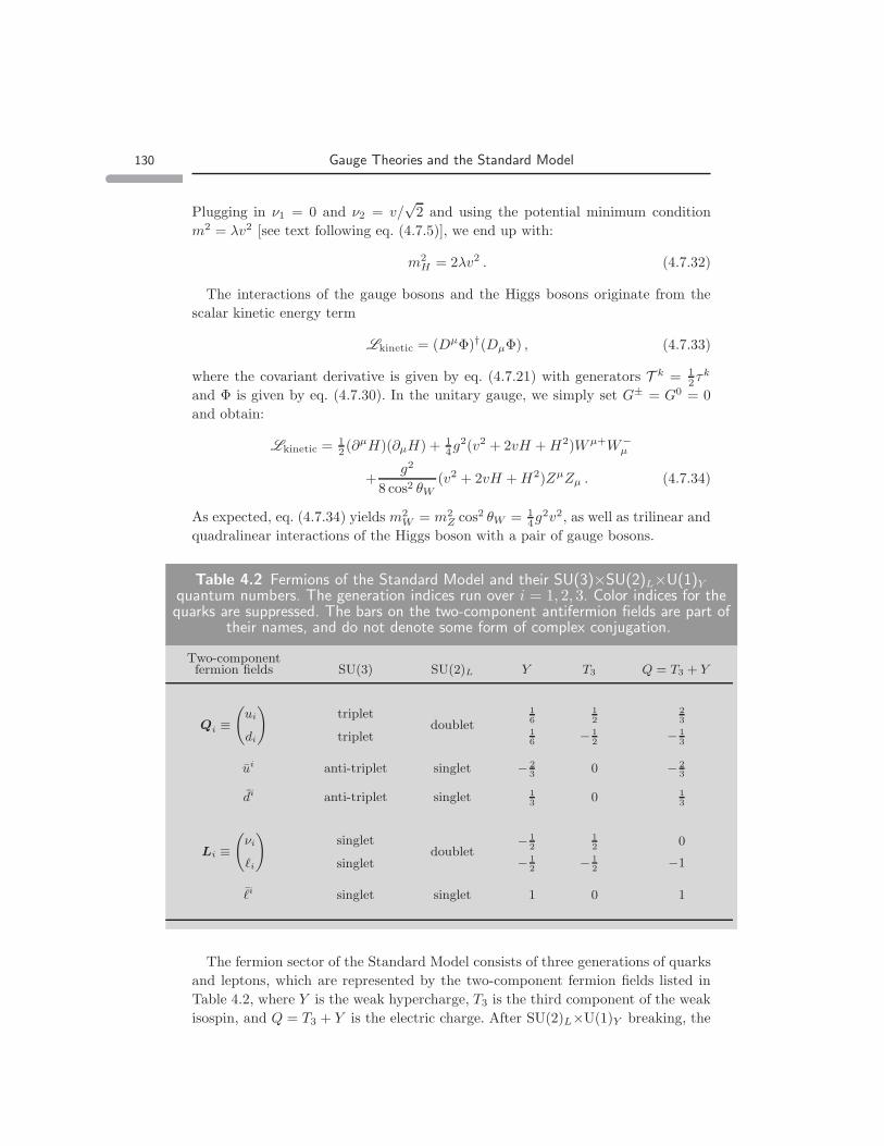
Table 4.2 Fermions of the Standard Model and their SU(3)×SU(2)L×U(1)Yquantum numbers. The generation indices run over i = 1, 2, 3. Color indices for thequarks are suppressed. The bars on the two-component antifermion fields are part of
their names, and do not denote some form of complex conjugation.
Two-componentfermion fields SU(3) SU(2)L Y T3 Q = T3 + Y
Qi ≡(ui
di
)triplet
tripletdoublet
16
16
12
− 12
23
− 13
ui anti-triplet singlet − 23
0 − 23
di anti-triplet singlet 13
0 13
Li ≡(νi
ℓi
)singlet
singletdoublet
− 12
− 12
12
− 12
0
−1
ℓi singlet singlet 1 0 1
The fermion sector of the Standard Model consists of three generations of quarks
and leptons, which are represented by the two-component fermion fields listed in
Table 4.2, where Y is the weak hypercharge, T3 is the third component of the weak
isospin, and Q = T3 + Y is the electric charge. After SU(2)L×U(1)Y breaking, the
131 The Standard Model of particle physics
quark and lepton fields gain mass in such a way that the above two-component
fields combine to make up four-component Dirac fermions:
Ui =
(ui
u†i
), Di =
(di
d†i
), Li =
(ℓi
ℓ†i
), (4.7.35)
while the neutrinos νi remain massless. The extension of the Standard Model to
include neutrino masses will be treated in Chapter 5.
Note that u, u, d, d, ℓ and ℓ are two-component fields, whereas the usual four-
component quark and charged lepton fields are denoted by capital letters U , D and
E. Consider a generic four-component field expressed in terms of the corresponding
two-component fields:
F =
(f
f †
). (4.7.36)
The electroweak quantum numbers of f are denoted by T f3 , Yf and Qf , whereas
the corresponding quantum numbers for f are T f3 = 0 and Qf = Yf = −Qf . Thus
we have the correspondence to our general notation [eq. (3.1.5)]
f ←→ χ, f ←→ η . (4.7.37)
The QCD color interactions of the quarks are governed by the following interac-
tion Lagrangian:
Lint = −gsAµaq†mi σµ(T a)mnqni + gsA
µa q
†ni σµ(T a)m
nqmi , (4.7.38)
summed over the generations i, where q is a (mass eigenstate) quark field, m and n
are SU(3) color triplet indices, Aµa is the gluon field (with the corresponding gluons
denoted by ga), and T a are the color generators in the triplet representation of
SU(3).
The electroweak interactions of the quarks and leptons are governed by the fol-
lowing interaction Lagrangian:
Lint = − g√2
[(u†iσµdi + ν†iσµℓi)W
+µ + (d†iσµui + ℓ†iσµνi)W
−µ
]
− g
cW
∑
f=u,d,ν,ℓ
{(T f3 − s2WQf)f †iσµfi + s2WQf
ˆf †iσµ ˆfi
}Zµ
−e∑
f=u,d,ℓ
Qf (f †iσµfi − ˆf †iσµ ˆfi)Aµ , (4.7.39)
where sW ≡ sin θW , cW ≡ cos θW , the hatted symbols indicate fermion interaction
eigenstates and i labels the generations. Before we perform any practical compu-
tations, we must convert from fermion interaction eigenstates to mass eigenstates.
In order to accomplish this step, we must first identify the quark and lepton mass
matrices.
In the electroweak theory, the fermion mass matrices originate from the fermion-
Higgs Yukawa interactions. The Higgs field of the Standard Model is a complex

132 Gauge Theories and the Standard Model
SU(2)L doublet of hypercharge Y = 12 , denoted by Φa, where the SU(2)L index
a = 1, 2 is defined such that Φ1 ≡ Φ+ and Φ2 ≡ Φ0 [cf. eq. (4.7.1)]. Here, the
superscripts + and 0 refer to the electric charge of the Higgs field, Q = T3 + Y ,
with Y = 12 and T3 = ± 1
2 . Since Φa is a complex field, its complex conjugate
Φ† a ≡(Φ− , (Φ0)†
)is an SU(2)L doublet scalar field with hypercharge Y = − 1
2 ,
where Φ− ≡ (Φ+)†. The SU(2)L×U(1)Y gauge invariant Yukawa interactions of the
quarks and leptons with the Higgs field are then given by:
LY = ǫab(Y u)ijΦaQbiuj − (Y d)
ijΦ
† aQaiˆdj − (Y ℓ)
ijΦ
† aLaiˆℓj + h.c., (4.7.40)
where ǫab is the antisymmetric invariant tensor of SU(2)L, defined such that ǫ12 =
−ǫ21 = +1. Using the definitions of the SU(2)L doublet quark and lepton fields
given in Table 4.2, one can rewrite eq. (4.7.40) more explicitly as:
−LY = (Y u)ij
[Φ0ui ˆu
j − Φ+di ˆuj]
+ (Y d)ij
[Φ−ui
ˆdj + Φ0∗diˆdj]
+(Y ℓ)ij
[Φ−νi
ˆℓj + Φ0∗ℓiˆℓj]
+ h.c. (4.7.41)
The Higgs fields can be written in terms of the physical Higgs scalar hSM and
Nambu-Goldstone bosons G0, G± as
Φ0 =1√2
(v + hSM + iG0) , (4.7.42)
Φ+ = G+ = (Φ−)† = (G−)†. (4.7.43)
where v = 2mW /g ≃ 246 GeV. In the unitary gauge appropriate for tree-level
calculations, the Nambu-Goldstone bosons become infinitely heavy and decouple.
We identify the quark and lepton mass matrices by setting Φ0 = v/√
2 and Φ+ =
Φ− = 0 in eq. (4.7.41):
(Mu)ij =v√2
(Y u)ij , (Md)ij =
v√2
(Y d)ij , (M ℓ)
ij =
v√2
(Y ℓ)ij .(4.7.44)
The neutrinos remain massless as previously indicated.
To diagonalize the quark and lepton mass matrices, we introduce four unitary
matrices for the quark mass diagonalization, Lu, Ld, Ru and Rd, and two unitary
matrices for the lepton mass diagonalization, Lℓ and Rℓ [cf. eq. (1.6.8)] such that
ui = (Lu)ijuj , di = (Ld)i
jdj , ˆui = (Ru)ij uj , ˆdi = (Rd)
ij dj ,(4.7.45)
ℓi = (Lℓ)ijℓj ,
ˆℓi = (Rℓ)ij ℓj , (4.7.46)
where the unhatted fields u, d, u and d are the corresponding quark mass eigenstates
and ν, ℓ and ℓ are the corresponding lepton mass eigenstates. The fermion mass
diagonalization procedure consists of the singular value decomposition of the quark
and lepton mass matrices:
LT
uMuRu = diag(mu , mc , mt) , (4.7.47)
LT
dMdRd = diag(md , ms , mb) , (4.7.48)
LT
ℓM ℓRℓ = diag(me , mµ , mτ ) , (4.7.49)

133 The Standard Model of particle physics
where the diagonalized masses are real and non-negative. Since the neutrinos are
massless, we are free to define the physical neutrino fields, νi, as the weak SU(2)
partners of the corresponding charged lepton mass eigenstate fields. That is,
νi = (Lℓ)ijνj . (4.7.50)
We can now write out the couplings of the mass eigenstate quarks and leptons to
the gauge bosons and Higgs bosons. Consider first the charged current interactions
of the quarks and leptons. Using eq. (5.2.49), it follows that u†iσµdi = Kiju†iσµdj ,
where
K = L†uLd (4.7.51)
is the unitary Cabibbo-Kobayashi-Maskawa (CKM) matrix [?].21 Due to eq. (4.7.50),
the corresponding leptonic CKM matrix is the unit matrix. Hence, the charged cur-
rent interactions take the form
Lint = − g√2
[Ki
ju†iσµdjW+µ + (K†)i
jd†iσµujW−µ + ν†iσµℓiW
+µ + ℓ†iσµνiW
−µ
],
(4.7.52)
where [K†]ij ≡ [Kji]∗. Note that in the Standard Model, u, d and ℓ do not couple
to the W±.
To obtain the neutral current interactions, we insert eqs. (5.2.49)–(4.7.50) into
eq. (4.7.39). All factors of the unitary matrices Lf and Rf (f = u, d, ℓ) cancel out,
and the resulting interactions are flavor-diagonal. That is, we may simply remove
the hats from the quark and lepton fields that couple to the Z and photon fields in
eq. (4.7.39). This is the well-known Glashow-Iliopoulos-Maiani (GIM) mechanism
for the flavor-conserving neutral currents [?].
The diagonalization of the fermion mass matrices is equivalent to the diagonal-
ization of the Yukawa couplings [cf. eqs. (4.7.44) and (4.7.47)–(4.7.49)]. Thus, we
define22
Yfi =√
2mfi/v , f = u, d, ℓ , (4.7.53)
where i labels the fermion generation. It is convenient to rewrite eqs. (4.7.47)–
(4.7.49) as follows:
(Lf )kj(Y f )km(Rf )mi = Yfiδ
ji , f = u, d, ℓ , (4.7.54)
with no sum over the repeated index i. Using the unitarity of Lf (f = u, d),
eq. (4.7.54) is equivalent to the following convenient form:
(Y fRf )ki = Yfi(L†f )i
k . (4.7.55)
21 The CKM matrix elements Vij as defined in ref. [?] are related by, for example, Vtb = K33 and
Vus = K12.
22 Boldfaced symbols are used for the non-diagonal Yukawa matrices, while non-boldfaced symbols
are used for the diagonalized Yukawa couplings.

134 Gauge Theories and the Standard Model
Inserting eqs. (5.2.49), (4.7.50) and (4.7.54) into eq. (4.7.41), the resulting Higgs-
fermion Lagrangian is flavor-diagonal:
Lint = − 1√2hSM
[Yuiuiu
i + Ydididi + Yℓiℓiℓ
i]
+ h.c. (4.7.56)
4.8 Parameter count of the Standard Model
The Standard Model Lagrangian appears to contain many parameters. However, not
all these parameters can be physical. One is always free to redefine the Standard
Model fields in an arbitrary manner. By suitable redefinitions, one can remove
some of the apparent parameter freedom and identify the true physical independent
parametric degrees of freedom.
To illustrate the procedure, let us first make a list of the parameters of the
Standard Model. First, the gauge sector consists of three real gauge couplings (g3, g2and g1) and the QCD vacuum angle (θQCD). The Higgs sector consists of one Higgs
squared-mass parameter and one Higgs self-coupling (m2 and λ). Traditionally, one
trades in the latter two real parameters for the vacuum expectation value (v =
246 GeV) and the physical Higgs mass. The fermion sector consists of three Higgs-
Yukawa coupling matrices yu, yd, and ye. Initially, yu, yd, and ye are arbitrary
complex 3× 3 matrices, which in total depend on 27 real and 27 imaginary degrees
of freedom.
But, most of these degrees of freedom are unphysical. In particular, in the limit
where yu = yd = ye = 0, the Standard Model possesses a global U(3)5 symmetry
corresponding to three generations of the five SU(3)×SU(2)×U(1) multiplets: (νm,
e−m)L, (ecm)L, (um, dm)L, (ucm)L, (dcm)L, where m is the generation label. Thus, one
can make global U(3)5 rotations on the fermion fields of the Standard Model to
absorb the unphysical degrees of freedom of yu, yd, and ye. A U(3) matrix can be
parameterized by three real angles and six phases, so that with the most general
U(3)5 rotation, we can apparently remove 15 real angles and 30 phases from yu,
yd, and ye. However, the U(3)5 rotations include four exact U(1) global symmetries
of the Standard Model, namely B and the three separate lepton numbers Le, Lµand Lτ . Thus, one can only remove 26 phases from yu, yd, and ye. This leaves 12
real parameters (corresponding to six quark masses, three lepton masses, 23 and
three CKM mixing angles) and one imaginary degree of freedom (the phase of the
CKM matrix). Adding up to get the final result, one finds that the Standard Model
possesses 19 independent parameters (of which 13 are associated with the flavor
sector).
23 The neutrinos in the Standard Model are automatically massless and are not counted as inde-
pendent degrees of freedom in the parameter count.
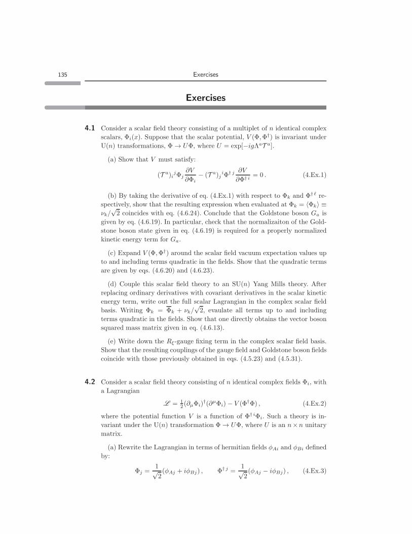
135 Exercises
Exercises
4.1 Consider a scalar field theory consisting of a multiplet of n identical complex
scalars, Φi(x). Suppose that the scalar potential, V (Φ,Φ†) is invariant under
U(n) transformations, Φ→ UΦ, where U = exp[−igΛaT a].
(a) Show that V must satisfy:
(T a)ijΦj
∂V
∂Φi− (T a)j
iΦ† j ∂V
∂Φ† i = 0 . (4.Ex.1)
(b) By taking the derivative of eq. (4.Ex.1) with respect to Φk and Φ† ℓ re-
spectively, show that the resulting expression when evaluated at Φk = 〈Φk〉 ≡νk/√
2 coincides with eq. (4.6.24). Conclude that the Goldstone boson Ga is
given by eq. (4.6.19). In particular, check that the normalizaiton of the Gold-
stone boson state given in eq. (4.6.19) is required for a properly normalized
kinetic energy term for Ga.
(c) Expand V (Φ,Φ†) around the scalar field vacuum expectation values up
to and including terms quadratic in the fields. Show that the quadratic terms
are given by eqs. (4.6.20) and (4.6.23).
(d) Couple this scalar field theory to an SU(n) Yang Mills theory. After
replacing ordinary derivatives with covariant derivatives in the scalar kinetic
energy term, write out the full scalar Lagrangian in the complex scalar field
basis. Writing Φk = Φk + νk/√
2, evaulate all terms up to and including
terms quadratic in the fields. Show that one directly obtains the vector boson
squared mass matrix given in eq. (4.6.13).
(e) Write down the Rξ-gauge fixing term in the complex scalar field basis.
Show that the resulting couplings of the gauge field and Goldstone boson fields
coincide with those previously obtained in eqs. (4.5.23) and (4.5.31).
4.2 Consider a scalar field theory consisting of n identical complex fields Φi, with
a Lagrangian
L = 12 (∂µΦi)
†(∂µΦi)− V (Φ†Φ) , (4.Ex.2)
where the potential function V is a function of Φ† iΦi. Such a theory is in-
variant under the U(n) transformation Φ→ UΦ, where U is an n×n unitary
matrix.
(a) Rewrite the Lagrangian in terms of hermitian fields φAi and φBi defined
by:
Φj =1√2
(φAj + iφBj) , Φ† j =1√2
(φAj − iφBj) , (4.Ex.3)

136 Gauge Theories and the Standard Model
and introduce the 2n-dimensional hermitian scalar field:
φ(x) =
(φA(x)
φB(x)
). (4.Ex.4)
Show that the Lagrangian is actually invariant under a larger symmetry group
O(2n), corresponding to the transformation φ → Oφ where O is a 2n × 2n
orthogonal matrix.
(b) Working in the complex basis, show that the Lagrangian [eq. (4.Ex.2)]
is invariant under the transformation:
Φi → UijΦj + Φ† j(V †)j
i , (4.Ex.5)
where U and V are complex n× n matrices, provided that the following two
conditions are satisfied:
(i) (U †U + V †V )ij = δi
j , (4.Ex.6)
(ii) V TU is an antisymmetric matrix . (4.Ex.7)
(c) Show that the 2n× 2n matrix
Q =
(Re(U + V ) − Im(U + V )
Im(U − V ) Re(U − V )
)(4.Ex.8)
is an orthogonal matrix if U and V satisfy eqs. (4.Ex.6) and (4.Ex.7). Prove
that any 2n× 2n orthogonal matrix can be written in the form of eq. (4.Ex.8)
by verifying that Q is determined by n(2n− 1) independent parameters.
(d) Use the results of parts (b) and (c) to conclude that if U is a unitary
n× n matrix, then the 2n× 2n matrix
QU =
(ReU − ImU
ImU ReU
)(4.Ex.9)
provides an explicit embedding of the subgroup U(n) inside O(2n). By writ-
ing QU = exp[−igΛaT a] and U = exp[−igΛaT a], show that T a is given by
eq. (4.6.9) in terms of the T a.
Likewise, define QV by taking U = 0 in Q [eq. (4.Ex.8)]. Show that QV also
provides an embedding of the subgroup U(n) inside O(2n). Prove that QU and
QV are in fact equivalent representations of U(n) by explicitly constructing
the similarity transformation such that S−1QUS is of the same form as QV(with U substituted for V ). Note that QU and QV depend implicitly on the
group element g ∈ U(n), whereas S is a fixed invertible matrix.
(e) Define the unitary matrix
A =
(In −iIniIn In
), (4.Ex.10)

137 Exercises
where In is the n × n identity matrix. Consider a real orthogonal 2n × 2n
matrix R that satisfies:
RTAR = A . (4.Ex.11)
Using an infinitesimal analysis (where R ≃ I + Z where Z is an infinitesimal
real antisymmetric 2n×2n matrix), prove that R provides an n⊕n∗ reducible
representation of U(n). Verify that both QU and QV satisfy the constraint
given by eq. (4.Ex.11)
(f) The natural embedding of the SO(2n) subgroup inside U(2n) can be
constructed by considering the matrix
U =
(U V ∗
V U∗
), (4.Ex.12)
where U and V satisfy eqs. (4.Ex.6) and (4.Ex.7). Verify that U is a unitary
matrix. Then, prove that Q and U provide equivalent representations of O(2n)
by explicitly constructing the similarity transformation U = P−1QP for some
fixed invertible matrix P (which is independent of the group element).
4.3 Repeat parts (a)–(d) of problem 2, under the assumption that Φ(x) is a
quaternionic-valued field.
(a) Show that an analogous analysis yields an explicit embedding of Sp(n)
as a subgroup of U(2n) [or equivalently as a subgroup of O(4n)].
(b) How does the fundamental representation of O(4n) decompose with
respect to the Sp(n) subgroup? How does the fundamental representation of
U(2n) decompose with respect to the Sp(n) subgroup?
4.4 Consider the spontaneous breaking of a gauge group G down to U(1). The
unbroken generatorQ = caTa is some real linear combination of the generators
of G.
(a) Prove that xb ≡ cb/gb is an (unnormalized) eigenvector of the vector
boson squared-mass matrix, M2ab, with zero eigenvalue.
(b) Suppose that Aµ is the massless gauge field that corresponds to the gen-
erator Q. Show that the covariant derivative can be expressed in the following
form:
Dµ = ∂µ + ieQAµ + . . . , (4.Ex.13)
where we have omitted terms in eq. (4.Ex.13) corresponding to all the other
138 Gauge Theories and the Standard Model
gauge bosons and
e =
[∑
a
(caga
)2]−1/2
. (4.Ex.14)
HINT: The vector boson mass matrix is diagonalized by an orthogonal trans-
formation OM2OT according to eq. (4.5.17). The rows of the matrix O are
constructed from the orthonormal eigenvectors of M2.
(c) Evaluate Q in the adjoint representation (i.e., Q = caTa, where the
(T a)bc = −ifabc are the generators of G in the adjoint representation). Show
that Qbcxc = 0, where xc is defined in part (a). What is the physical inter-
pretation of this result?
(d) Prove that the commutator [Q,M2] = 0, where Q is the unbroken U(1)
generator in the adjoint representation and M2 is the gauge boson squared-
mass matrix. Conclude that one can always choose the eigenstates of the gauge
boson squared-mass matrix to be states of definite unbroken U(1)-charge.
(e) Apply the results of part (b) to the spontaneous breaking of SU(2)×U(1)Yto U(1)EM in the Standard Model of electroweak interactions. Show that
eq. (4.Ex.14) reproduces eq. (4.7.11).
4.5 The generators of SU(2)×U(1) in the hypercharge-one SU(2) doublet repre-
sentation can be expressed as 4× 4 matrices by using the real representation
of eq. (4.6.9).
(a) Using the explicit form for this real representation, derive the gauge bo-
son squared-mass matrix. Diagonalize the mass matrix and explicitly identify
the real antisymmetric matrix generators La.
(b) Use eq. (4.5.24) to obtain the Goldstone bosons and identify the physical
Higgs boson.
(c) Using the real representation, write down an explicit form for DµΦ as
a four-dimensional column vector. Then, evaluate eq. (4.7.33) in the unitary
gauge and verify the results of eq. (4.7.34).
4.6 Derive the interaction Lagrangian for the charged and neutral Nambu-Goldstone
bosons and the fermions of the Standard Model and verify that
Lint = Yui[K]ijdj u
iG+ − Ydi[K†]ijuj d
iG− − YℓiνiℓiG−
+i√2
[Ydidid
i − Yuiuiui + Yℓ iℓiℓi]G0 + h.c. , (4.Ex.15)
where K is the CKM matrix and Yfi (for f = u, d, ℓ) is given by eq. (4.7.53).

139 Exercises
4.7 In Section 4.7, we examined in detail the structure of a spontaneously broken
SU(2)×U(1)Y gauge theory, in which the symmetry breaking was due to the
vacuum expectation value of a Y = 12 , SU(2) doublet of complex scalar fields.
In this problem, we will replace this multiplet of scalar fields with a different
representation.
(a) Consider a spontaneously broken SU(2)×U(1)Y gauge theory with a
Y = 0, SU(2) triplet of real scalar fields. Assume that the electrically neu-
tral member of the scalar triplet acquires a vacuum expectation value. After
symmetry breaking, identify the subgroup that remains unbroken. Compute
the vector boson masses and the physical Higgs scalar masses in this model.
Deduce the Feynman rules for the three-point interactions among the Higgs
and vector bosons.
HINT: Since the triplet of scalar fields corresponds to the adjoint represen-
tation of SU(2), the corresponding SU(2) generators that act on the triplet
of scalar fields can be chosen to be (T a)bc = −iǫabc. The hypercharge opera-
tor annihilates the Y = 0 fields. Define La = igaTa, and follow the methods
outlined in Section 4.5.4.
(b) Consider a spontaneously broken SU(2)×U(1)Y gauge theory with a
Y = 1, SU(2) triplet of complex scalar fields. Again, assume that the elec-
trically neutral member of the scalar triplet acquires a vacuum expectation
value. After symmetry breaking, identify the subgroup that remains unbro-
ken. Compute the vector boson masses and the physical Higgs scalar masses
in this model.
(c) If both doublet and triplet Higgs fields exist in nature, what does this
exercise imply about the parameters of the Higgs Lagrangian?
References
[1] John C. Taylor, Gauge Theories of Weak Interactions, (Cambridge University
Press, Cambridge, England, 1976).
[2] Steven Weinberg, The Quantum Theory of Fields: Volume II—Modern Appli-
cations, (Cambridge University Press, Cambridge, England, 1996).
[3] L. Oraifeartaigh, Group Structure of Gauge Theories (Cambridge University
Press, Cambridge, England, 1986).
[4] S. Weinberg, Phys. Rev., D7 (1973) 1068.
[5] David Bailin and Alexander Love, Introduction to Gauge Field Theory (Insti-
tute of Physics Publishing, London, 1993).
[6] Dima Bardin and Giampiero Passarino, The Standard Model in the Making:
Precision Study of the Electroweak Interactions (Oxford University Press, Ox-
ford, England, 1999).
[7] For a review, see E.S. Abers and B.W. Lee, Physics Reports, 9C (1973) 1.
[8] Kerson Huang, Quarks, Leptons and Gauge Fields (World Sicentific Publish-
ing, Singapore, 1992).
140