NIST Measurement Services:

Gas Flowmeter Calibrations with the 34 L and 677 L PVTt Standards NIST Special Publication 250-63

John D. Wright, Aaron N. Johnson, Michael R. Moldover, and Gina M. Kline U. S. Department of Commerce Technology Administration National Institute of Standards and Technology

Table of Contents Gas Flowmeter Calibrations with the 34 L and 677 L PVTt Standards Abstract ...................................................................................................................... 1 1 Introduction............................................................................................................ 2 2 Description of Measurement Services ................................................................... 4 3 Procedures for Submitting a Flowmeter for Calibration........................................ 7 4 Pressure, Volume, Temperature, and time (PVTt) Standards ................................ 7 5 Design and Operation of the PVTt Standard........................................................ 11

5.1 Average Temperature of the Collected Gas ...............................................11 5.2 Mass Change in the Inventory Volume.......................................................16 5.3 Measurement of the Tank and Inventory Volumes .....................................24

6 Uncertainty Analysis of the 34 L and 677 L PVTt Flow Standards..................... 27 6.1 Techniques for Uncertainty Analysis .........................................................28 6.2 Mass Flow Uncertainty ..............................................................................31 6.3 Pressure ......................................................................................................33 6.4 Temperature................................................................................................36 6.5 Compressibility, Molecular Weight, and Gas Constant .............................39 6.6 Density........................................................................................................42 6.7 Collection Time..........................................................................................43 6.8 Volume of the 677 Liter Collection Tank (Gravimetric Method)..............44 6.9 Volume of the 34 Liter Collection Tank (Volume Expansion Method) ....48 6.10 Inventory Volume.....................................................................................50

7 Experimental Verification of the Uncertainty of the 34 L and 677 L PVTt Gas Flow Standards......................................................................................................... 55

7.1 Comparison of the 34 L and 677 L Flow Standards...................................56 7.2 Multiple Diversions in the 677 L Flow Standard .......................................59

8 Summary .............................................................................................................. 60 9 References............................................................................................................ 62 Appendix: Sample Calibration Report

i

Abstract This document provides a description of the 34 L and 677 L pressure, volume,

temperature, and time (PVTt) primary gas flow standards operated by the National

Institute of Standards and Technology (NIST) Fluid Flow Group. These facilities are

used to provide gas flowmeter calibration services as reported in NIST Special

Publication 250 [Marshall 1998] for Test Numbers 18010C and 18050C. The PVTt

standard uses two collection tanks and two diverter valve systems to perform gas

flowmeter calibrations between 1 L/min and 2000 L/min (the reference temperature and

pressure conditions are 293.15 K and 101.325 kPa). The standard measures flow by

collecting gas in a tank of known volume during a measured time interval. The

uncertainty of the flow measurement is between 0.02 % and 0.05 % (k = 2 or

approximately 95 % confidence level), depending on the gas used and where in the flow

range the facilities are being used.

We provide an overview of the gas flow calibration service and the procedures for

customers to submit their flowmeters to NIST for calibration. We describe the significant

and novel features of the standard and analyze its uncertainty. The gas collection tanks

have a small diameter and are immersed in a uniform, stable, thermostatted water bath.

The collected gas achieves thermal equilibrium rapidly, and the uncertainty of the

average gas temperature is only 7 mK (22 × 10-6 T). A novel operating method leads to

essentially zero mass change in and very low uncertainty contributions from the

inventory volume.

Gravimetric and volume expansion techniques were used to determine the tank and the

inventory volumes. Gravimetric determinations of collection tank volume made with

nitrogen and argon agree with a standard deviation of 16 × 10-6 VT. The largest source of

uncertainty in the flow measurement is drift of the pressure sensor over time, which

contributes a relative standard uncertainty of 60 × 10-6 to the determinations of the

volumes of the collection tanks and to the flow measurements. Throughout the range 3

L/min to 110 L/min, flows were measured independently using the 34 L and the 677 L

collection systems, and the two systems agreed within a relative difference of 150 × 10-6.

1

Double diversions were used to evaluate the 677 L system over a range of 300 L/min to

1600 L/min, and the relative differences between single and double diversions were less

than 75 × 10-6.

Key words: calibration, correlated uncertainty, flow, flowmeter, gas flow standard,

inventory volume, PVTt standard, mass cancellation, meter, sensor response, uncertainty.

1 Introduction

Calibrations of gas flowmeters are performed with primary standards [ISO 1993] that are

based on measurements of more fundamental quantities, such as length, mass, and time.

Primary flow calibrations are accomplished by collecting a measured mass or volume of

the flowing fluid over a measured time interval under approximately steady state

conditions of flow, pressure, and temperature at the meter under test. The flow measured

by the primary standard is computed along with the average of the flow indicated by the

meter under test during the collection interval. All of the quantities measured in

connection with the calibration standard (i.e., temperature, pressure, time, etc.) are

traceable to established national standards. A gas calibration facility consists of a fluid

source (e.g., an air compressor or compressed gas cylinders), a test section that provides

stable thermodynamic conditions and a fully developed flow profile, and a system for

diverting and timing the collection of a quantity of the fluid.

NIST offers calibrations of gas flowmeters in order to provide traceability to flowmeter

manufacturers, secondary flow calibration laboratories, and flowmeter users. For a

calibration fee, NIST calibrates a customer’s flowmeter and delivers a calibration report

that documents the calibration procedure, the calibration results, and their uncertainty.

The flowmeter and its calibration results may be used in different ways by the customer.

The flowmeter is often used as a transfer standard to perform a comparison of the

customer’s primary standards to the NIST primary standards so that the customer can

establish traceability, validate their uncertainty analysis, and demonstrate proficiency.

2

Customers with no primary standards use their NIST calibrated flowmeters as working

standards or reference standards in their laboratory to calibrate other flowmeters.

The Fluid Flow Group of the Process Measurements Division (part of the Chemical

Science and Technology Laboratory) at NIST provides gas flow calibration services over

a range of 1 L/min to 77600 L/min.∗ Table 1 presents the flow ranges covered by the

primary gas flow standards in the Fluid Flow Group. Flows from 900 L/min to 77600

L/min can be measured with a 26 m3 PVTt standard that was built in the late 1960’s and

has been upgraded several times [Olsen and Baumgarten 1971, Johnson et al. 2003].

Flows of 1 L/min or less can be calibrated by the NIST Pressure and Vacuum Group.

Table 1. Primary gas flow calibration capabilities within the NIST Fluid Flow Group.

Flow

Standard

Flow Range

(L/min)

Gas

Pressure Range

(kPa)

Uncertainty

(k = 2) (%)

1 - 100 N2 100 – 7000 0.03 – 0.04

1 - 100 Air 100 - 1700 0.05

1 - 100 CO2 100 - 4000 0.05

1 - 100 Ar 100 - 7000 0.05

34 L PVTt

1 - 100 He 100 - 7000 0.05

10 - 150 N2 100 - 800 0.02 – 0.03 677 L PVTt

10 -2000 Air 100 - 1700 0.05

26 m3 PVTt 860 - 77600 Air 100 - 800 0.13

This document describes the theory, methods of operation, and uncertainty of the 34 L

and 677 L PVTt primary standards that cover the 1 L/min to 2000 L/min flow range.

From the late 1960’s to 2002, this flow range was covered by a set of three mercury-

sealed piston provers and two bell provers [Wright and Mattingly 1998]. The 34 L and

677 L PVTt standards were completed in 2002, and for a period of one year we used both

∗ Reference conditions of 293.15 K and 101.325 kPa are used throughout this document for volumetric flows.

3

the old and the new primary standards for customer calibrations. In 2003, the new

primary standards and their uncertainty statements were sufficiently validated [Wright

2003A], and we began using the new standards alone to calibrate customers’ flowmeters.

The PVTt standard is ideally suited for the calibration of critical flow venturis (CFV’s)

since they provide pressure isolation and provide a well defined boundary for the

inventory volume. A set of NIST CFV’s, calibrated by the PVTt standards are used as

working standards in another calibration facility called the Working Gas Flow Standard

(WGFS). The WGFS provides calibrations, particularly for laminar flowmeters, in which

the reference flow is measured with uncertainty of 0.1% or less. The methods and

uncertainty analysis for the WGFS are covered in a separate document.

2 Description of Measurement Services

Customers should consult the web address www.nist.gov/fluid_flow to find the most

current information regarding our calibration services, calibration fees, technical contacts,

and flowmeter submittal procedures.

NIST uses the PVTt primary standards described herein to provide gas flowmeter

calibrations for flows between 1 L/min and 2000 L/min. The facility has been used at

flows as low as 0.025 L/min, but calibrations below 1 L/min should be discussed with the

technical contacts before a flowmeter is submitted for such low flows.

The gases available for calibrations in the 34 L PVTt standard are dry air, nitrogen,

carbon dioxide, argon, and helium. The source of air, at pressures up to 1700 kPa, is an

oil-free reciprocating compressor and a refrigeration drier. The dew point temperature of

the dried air is 250 K so the mole fraction of water in the air is 0.08 %. Nitrogen (at

pressures up to 800 kPa and purity of 99.998%) is supplied by liquid nitrogen dewars.

Higher pressures of nitrogen as well as argon, carbon dioxide, and helium gas can be

supplied from compressed gas cylinders. Other non-toxic, non-corrosive gases can be

accommodated upon customer request. While other gases are certainly feasible in the 677

4

L PVTt standard, gases are practically limited to air from the compressor and nitrogen

from dewars since a very large number of gas cylinders would be necessary to provide

gas at 2000 L/min. The gas temperatures are nominally room temperature.

Readily available fittings for the installation of flowmeters in the 34 L and 677 L PVTt

standards are Swagelok∗ (1/8” to 1”), A/N 37 degree flare (1/4” to 1”), national pipe

thread or NPT (1/8” to 3”), VCR (1/4” and 1/2”), and VCO (1/2” and 1”).

Meters can be tested if the flow range, gas, and piping connections are suitable, and if the

system to be tested has precision appropriate for calibration with the NIST flow

measurement uncertainty. The vast majority of flowmeters calibrated in the gas flow

calibration service are either critical flow venturis (critical nozzles) or laminar

flowmeters since these are presently regarded as the best candidates for transfer and

working standards by the gas flow metrology community [Wright 2003B]. Other meter

types that we have tested include positive displacement meters, roots meters, rotary gas

meters, thermal mass flowmeters, and turbine meters. Meter types with calibration

instability significantly larger than the primary standard uncertainty should not be

calibrated with the NIST standards for economic reasons. For example, a rotameter for

which the float position is read by the operator’s eye normally cannot be read with

precison any better than 1 %. It is not practical to pay thousands of dollars to obtain

0.05 % or less uncertainty flow data from NIST for such a flowmeter when 0.5% data is

perfectly adequate and available from other laboratories at significantly lower cost.

A normal flow calibration performed by the NIST Fluid Flow Group consists of five

flows spread over the range of the flowmeter. For a CFV, typical calibration set points

are at 200 kPa, 300 kPa, 400 kPa, 500 kPa, and 600 kPa. A laminar flowmeter is

normally calibrated at 10 %, 25 %, 50 %, 75 %, and 100 % of the meter full scale. At

each of these flow set points, three (or more) flow measurements are made with the PVTt

∗ Certain commercial equipment, instruments, or materials are identified in this paper to foster understanding. Such identification does not imply recommendation or endorsement by the National Institute of Standards and Technology, nor does it imply that the materials or equipment identified are necessarily the best available for the purpose.

5

standard. The same set point flows are tested on a second occasion, but the flows are

tested in decreasing order instead of the increasing order of the first set. Therefore, the

final data set consists of six (or more) primary flow measurements made at five flow set

points, i.e., 30 individual flow measurements. The sets of three measurements can be

used to assess repeatability, while the sets of six can be used to assess reproducibility. For

further explanation, see the sample calibration report that is included in this document as

an appendix. Variations on the number of flow set points, spacing of the set points, and

the number of repeated measurements can be discussed with the NIST technical contacts.

However, for data quality assurance reasons, we rarely will conduct calibrations

involving fewer than three flow set points and two sets of three flow measurements at

each set point.

The Fluid Flow Group prefers to present flowmeter calibration results in a dimensionless

format that takes into account the physical model for the flowmeter type [Wright 1998].

The dimensionless approach facilitates accurate flow measurements by the flowmeter

user even when the conditions of usage (gas type, temperature, pressure) differ from the

conditions during calibration. Hence for a CFV calibration, the calibration report will

present Reynolds number and discharge coefficient and for a laminar flowmeter, a report

presents the viscosity coefficient and the flow coefficient. In order to calculate the

uncertainty of these flowmeter calibration factors, we must know the uncertainty of the

standard flow measurement as well as the uncertainty of the instrumentation associated

with the meter under test (normally absolute pressure, differential pressure, and

temperature instrumentation). We prefer to connect our own instrumentation

(temperature, pressure, etc.) to the meter under test since they have established

uncertainty values based on calibration records that we would not have for the customer’s

instrumentation. In some cases, it is impractical to install our own instrumentation on the

meter under test and the meter under test outputs flow. In these cases, we provide a table

of flow indicated by the meter under test, flow measured by the NIST standard, and the

uncertainty of the NIST flow value.

6

3 Procedures for Submitting a Flowmeter for Calibration

The Fluid Flow Group follows the policies and procedures described in Chapters 1, 2,

and 3 of the NIST Calibration Services Users Guide [Marshall 1998]. These chapters can

be found on the internet at the following addresses:

http://ts.nist.gov/ts/htdocs/230/233/calibrations/Policies/policy.htm,

http://ts.nist.gov/ts/htdocs/230/233/calibrations/Policies/domestic.htm, and

http://ts.nist.gov/ts/htdocs/230/233/calibrations/Policies/foreign.htm.

Chapter 2 gives instructions for ordering a calibration for domestic customers and has the

sub-headings: A.) Customer Inquiries, B.) Pre-arrangements and Scheduling, C.)

Purchase Orders, D.) Shipping, Insurance, and Risk of Loss, E.) Turnaround Time, and

F.) Customer Checklist. Chapter 3 gives special instructions for foreign customers. The

web address www.nist.gov/fluid_flow has information more specific to the gas flow

calibration service, including the technical contacts in the Fluid Flow Group, fee

estimates, and turnaround times.

4 Pressure, Volume, Temperature, and time (PVTt) Standards

PVTt systems have been used as primary gas flow standards by NIST and other

laboratories for more than 30 years [Olsen and Baumgarten 1971, Kegel 1995, Ishibashi

et al. 1985, Wright 2001]. The PVTt systems at NIST consist of a flow source, valves for

diverting the flow, a collection tank, a vacuum pump, pressure and temperature sensors,

and a critical flow venturi (CFV) which isolates the meter under test from the pressure

variations in the downstream piping and tank (see Fig. 1).

7

Figure 1. Arrangement of equipment in a PVTt system.

The process of making a PVTt flow measurement normally entails the following steps:

1. Close the tank valve, open the bypass valve, and establish a stable flow through the

CFV.

2. Evacuate the collection tank volume (VT) with the vacuum pump.

3. Wait for pressure and temperature conditions in the tank to stabilize and then acquire

initial values for the tank ( and iTP i

TT ). These values will be used to calculate the

initial density and the initial mass of gas in the tank ( ). iTm

4. Close the bypass valve and, during the “dead-end time” when both the bypass and

tank valves are fully closed, choose a start time ( ). At the same time, acquire the

initial pressure and temperature in the inventory volume ( and T ). These values

will be used along with the equation of state for the gas and the inventory volume (V

it

m

iIP i

I

I)

to obtain an initial mass in the inventory volume ( ). Shortly after the bypass valve

is fully closed, open the tank valve.

iI

5. Wait for the tank to fill to a prescribed upper pressure and then close the tank valve

and choose the stop time ( ) during the dead-end time. At the same time, acquire

the pressure and temperature in the inventory volume ( and T ) and hence the

final mass in the inventory. Open the bypass valve.

ftf

IP fI

8

6. Wait for stability and then acquire and and hence . f

TP fTT f

Tm

By writing a mass balance for the control volume composed of the inventory and tank

volumes (see the volume defined by the dashed line in Fig. 1), one can derive an equation

for the average mass flow during the collection time:

if

ifif )()(tt

mmmmm IITT

−−+−

=& , (1)

or, neglecting the volume changes between the initial and final conditions:

( ) ( )if

ifif

ttVVm IIITTT

−−+−

=ρρρρ

& , (2)

where ρ is the gas density determined via a real gas equation of state, ( ) ZRTPM=ρ ,

where M is the gas molecular weight, R is the universal gas constant, and Z is the

compressibility factor.

The start and stop times can be chosen at any point during the dead-end time as long as

the inventory conditions are measured coincidentally. Why is this true? Implicit in the

PVTt basis equation (Eq. 2) are two requirements: 1) the measurement of the initial and

final densities must be coincident with the measurement of the start and stop times and 2)

there must not be any other sources or sinks of mass flow to the control volume. The

second condition is met for the entire time that the bypass valve is fully closed, including

the start and stop dead-end times. It is not necessary that the initial and final

determinations of the mass in the collection tank be done coincidentally with the start and

stop times because the tank is free of leaks and it is advantageous to measure these mass

values when the tank conditions have reached equilibrium. The freedom to choose the

start and stop times from within the dead-end time intervals allows one to choose times

where the initial and final inventory densities match, giving essentially zero mass change

9

in the inventory volume ( ) and extremely good cancellation of certain correlated

inventory uncertainties.

Im∆

The PVTt measurement process can be performed in a “blow down” mode also, where

initial and final values of the mass in a tank that is the source of flow instead of the

collector of flow are utilized. Such a system has the advantage that a small compressor

can be used to charge a large pressure vessel over a long period of time allowing one to

achieve very large flows relatively inexpensively. The blow down method has the

disadvantage that it is more difficult to maintain stable pressure and temperature

conditions at the meter under test since the high-side pressure of the flow control

throttling process is changing continuously as the tank discharges.

The bypass and tank valves can be operated with valve overlap, i.e. where one valve

begins to open before the other is fully closed, or with zero overlap, where one is

completely closed before the other begins to open (as described above) [Harris 1980].

With zero overlap, there is no question about lost or extra mass occurring during the

diversion. For instance, if the tank is at an initial pressure less than atmospheric, when

both valves are partially open, flow can enter the tank from the room instead of through

the meter under test. Zero overlap avoids this possibility. For a zero overlap system it is

important that any valve design be fast acting. There is a short period of time during the

actuation of the diverter valves during which both valves are closed (the “dead end” time)

and the mass of gas that passed through the critical venturi accumulates in the inventory

volume. The mass accumulation leads to a pressure rise in the inventory volume that will

depend on the mass flow, the size of the inventory volume, and the dead end time of the

diverter valves. The pressure in the inventory must not be permitted to reach a high

enough level that the flow at the venturi is no longer critical, lest pressure perturbations

reach the meter under test and disrupt the steady state flow conditions at the meter.

10

5 Design and Operation of the PVTt Standard Experience with a previous, 26 m3 PVTt flow standard at NIST indicated that

improvements in temperature and pressure instrumentation as well as in the design and

operation of the new system would be necessary in order to achieve an uncertainty of

0.05 % or better [Johnson et al. 2003]. In the following three sections we will describe

aspects of the design and operation of the new flow standard that are important to achieve

this low uncertainty. The first of these sections describes the measurement of the average

temperature of the collected gas. A subsequent section describes the procedures that

minimize the uncertainty of the mass change in the inventory volume, and the last section

describes the determination of the tank and inventory volumes.

5.1 Average Temperature of the Collected Gas

One of the most important sources of uncertainty in a PVTt flow standard is the

measurement of the average temperature of the gas in the collection tank, particularly

after filling. The evacuation and filling processes lead to cooling and heating of the gas

within the volume due to flow work and kinetic energy phenomena [Wright and Johnson

2000]. The magnitude of the effect depends on the flow; however, the temperature rise in

an adiabatic tank can be 10 K or more. Hence, immediately after filling and evacuation,

significant thermal gradients exist within the collected gas. For a large tank, the

equilibration time for the gas temperature can be many hours. If the exterior of the tank

has non-isothermal or time varying temperature conditions, stratification and non-

uniform gas temperatures will persist even after many hours [Johnson et al. 2003].

11

Figure 2. A schematic of the PVTt collection tanks, water bath, duct, and temperature

control elements.

In this work, we avoided long equilibration times and the difficult problem of measuring

the average temperature of a non-uniform gas by designing the collection tanks for rapid

equilibration of the collected gas and by immersing the tanks in a well-mixed,

thermostatted, water bath (see Fig. 2 and Fig. 3). There are two control volumes, a 34 L

collection tank and a 677 L collection tank. Because the equilibration of the 677 L tank is

slower, we consider it here. The 677 L tank is composed of eight, cylindrical, 2.5 m

long, stainless steel shells connected in parallel by a manifold. Each shell has a wall

thickness of l = 0.6 cm and an internal radius of a = 10 cm. Because all of the collected

gas is within 10 cm of a nearly isothermal shell, the gas temperature quickly equilibrates

with that of the bath. After the collected gas equilibrates with the bath, the gas

temperature is determined by comparatively simple measurements of the temperature of

the recirculating water. Remarkably, the water temperature measurements made with 14

sensors had a standard deviation of only 0.4 mK during a typical, 20-minute-long,

equilibration interval. In the next section, we describe the bath; in the section after that,

we discuss the equilibration of the collected gas.

12

Large diverter valves Small diverter valves

677 L collection tank manifold

Heating, cooling, and mixing elements

34 L collection tank

Figure 3. A photograph of the two PVTt collection tanks submerged in the temperature

controlled water bath.

5.1.1 The Water Bath

The water bath is a rectangular trough 3.3 m long, 1 m wide, and 1 m high. Metal frames

immersed in the tank support all the cylindrical shells and a long duct formed by four

polycarbonate sheets. The duct surrounds the top, bottom, and sides of the shells:

however, both ends of the duct are unobstructed. At the upstream end of the bath, the

water is vigorously stirred and its temperature is controlled near the temperature of the

room (296.5 K) using controlled electrical heaters and tubing cooled by externally

refrigerated, circulated water. A propeller pushes the vigorously stirred water through the

duct along the collection tanks. When the flowing water reaches the downstream

(unstirred) end of the trough, it flows to the outsides of the duct and returns to the stirred

13

volume through the unobstructed, 10 cm thick, water-filled spaces between the duct and

the sides, the top, and the bottom of the rectangular tank.

297.286

297.287

297.288

297.289

297.29

0 10

Time (min)

T (K

)

20

Figure 4. Temperature data for 14 thermistors distributed in the water bath.

The uniformity and stability of the water temperature was studied using 14 thermistors.

The thermistors were bundled together and zeroed at one location in the water bath.

Then, they were distributed throughout the water bath. Figure 4 plots data recorded at 5 s

intervals from these 14 thermistors. Nearly all of the data in Fig. 4 is within ± 1 mK of

their mean and the standard deviation of the data from their mean is only 0.4 mK. The

largest temperature transients occur where the mixed water enters the duct, indicating

incomplete mixing. The tank walls attenuate these thermal transients before reaching the

collected gas. Thus, after equilibration, the non-uniformity of the water bath and the

fluctuations of the average gas temperature are less than ± 1 mK (3 × 10-6 T).

5.1.2 Equilibration of the Collected Gas

For design purposes, we estimated the time constant (τgas) that characterizes the

equilibration of the gas within the collection tank after the filling process. The estimate

considers heat conduction in an infinitely long, isotropic, “solid” cylinder of radius a

[Carslaw and Jaeger 1946]. For the slowest, radially symmetric heat mode,

14

gasτ = (a/2.405)2/DT, where DT is the thermal diffusivity of the gas. This estimate gives

gasτ = 80 s for nitrogen in the 677 L tank. This estimate for τgas is too large insofar as it

neglects convection, conduction through the ends of the tanks, and the faster thermal

modes, all of which hasten equilibration. The time constants for heat to flow from the gas

through the tank walls and the time constant for a hot or cold spot within a wall to decay

have been calculated and found to be less than a second. Therefore, we expect the

collected gas to equilibrate with a time constant of 80 s or less.

Figure 5. The equilibration of pressure and temperature immediately following a filling

of the 34 L tank at 25 L/min.

The equilibration of the collected gas was observed by using the tank as a constant-

volume gas thermometer. After the tank valve was closed, the pressure of the collected

gas was monitored, as shown in Fig. 5. Our analysis of data such as those in Fig. 5 leads

to the experimental values gasτ of less than 60 s for both the 677 L and 34 L tanks, in

reasonable agreement with the estimates. The measured time constant and Fig. 5 show

that a wait of 20 minutes guarantees that the collected gas is in equilibrium with the bath,

within the resolution of the measurements.

15

The manifold linking the 8 cylindrical shells is completely immersed in the water bath.

Thus, the gas in the manifold quickly equilibrates to the bath temperature as well.

However, each collection system has small, unthermostatted, gas filled volumes in the

tubes that lead from the collection tanks to the diverter valves, the pressure transducers,

etc. In Section 6.4.1, we show the possible temperature variations of these small,

unthermostatted volumes make very small contributions to the uncertainty of the gas

temperature and the flow measurements.

5.2 Mass Change in the Inventory Volume

5.2.1 Overview and Strategy

As outlined in Section 4, the start time ti and the stop time t f used in Eqs. 1 and 2 are

chosen to occur during the brief “dead-end times” (< 100 ms) when both the tank valve

and the bypass valve are closed, i.e., we use a “zero overlap” diversion [Harris and

Johnson 1990]. This choice has the advantage of clear mass balance accountability for

all the gas flowing through the critical flow venturi during both diversions and the tank

filling. Unfortunately, it is difficult to determine either m or m and hence the change in

mass within the inventory volume accurately (especially at high flows) because both the

pressure and the temperature in the inventory volume rise rapidly as the flow through the

critical venturi accumulates in the inventory volume (see Fig. 6).

fI

iI

Our strategy for dealing with the inventory mass change has two elements. First, by

design, the inventory volume VI is much smaller than the collection tank volume VT. (For

the 34 L system, VT /VI = 500; for the 677 L system, VT /VI = 700.) Thus, the uncertainty

of mass flow is relatively insensitive to uncertainty in and m since both are small

compared with the total mass of collected gas. Second, we choose t

fIm i

I

i near the end of the

dead-end time and we chose t f such that P(ti) = P(t f). These choices define a “mass

cancellation” method: since the initial and final inventory densities are essentially equal,

∆mI is nearly zero. In fact, we will assume that ∆mI is zero and consider the quantity only

in terms of flow measurement uncertainty, not as part of the flow calculation. Symmetry

16

of the inventory transients (see Fig. 7) and the mass cancellation method also give

uncertainty benefits due to high correlation in the uncertainties of pressure and

temperature measurements for ∆mI .

We tested our strategy for choosing ti and t f for both the 34 L and the 677 L flow

standards. (See Section 7 for details of these tests.) To test the 34 L system, we collected

identical flows spanning the range 3 L/min < < 100 L/min in both the small and the

large tanks, using the large tank as a reference for the small tank since its inventory

uncertainties are quite small in this flow range. To test the 677 L collection system, we

collected identical flows in the 677 L tank following two different protocols. In the first

protocol, the inventory volume was dead-ended at the beginning and end of the collection

interval in the usual manner. In the second protocol the collection interval was divided

into two subintervals, which doubled

m&

Im∆ and allowed assessment of its uncertainty

contribution.

These tests indicate uncertainties due to the inventory volume that are proportional to

flow as would be expected based on a thermodynamic model of the inventory pressure

and temperature transients. If the inventory uncertainties are considered to arise from

uncertainty in the collection time, the inventory mass change uncertainty found

experimentally for the 34 L system was u mIm &×=∆ ms4 (200 × 10-6 for its maximum

flow). For the 677 L system, single and double diversions changed the flow measurement

by 75 × 10

m&

-6 or less. m&

In the remainder of this section, we describe conditions within the inventory volume

during the dead-end times using both a model and measurements. The measurements

show that T(t) and P(t) are nearly the same during the start and stop dead-end times.

Finally, we show that is insensitive to the exact choice of tIm∆ i, provided that the

condition P(t i) = P(t f) is applied near the end of the dead-end time.

17

Figure 6. Experimentally measured data (25 L/min in the 34 L tank) and thermodynamic

model predictions for zero and non-zero sensor time constants. The model outputs

demonstrate that neglect of sensor response causes significant error in the measurement

of inventory conditions.

5.2.2 Conditions within the Inventory Volume

Figure 6 displays the time dependent temperature T(t) and pressure P(t) in the inventory

volume of the smaller collection system at a typical collection rate ( m = 25 L/min;

collection time = 82 s). The time t = 0 in Fig. 6 is defined by the signal indicating that

the valve is fully closed. The triangles (τ = 0) in Fig. 6 were calculated from the lumped-

parameter, thermodynamic model developed by Wright and Johnson [2000]. The model

assumes a constant mass flow at the entrance to the inventory volume. The model

&

m&

18

neglects heat transport from the gas to the surrounding structure and non-uniform

conditions, such as the jet entering the volume. For Fig. 6, T(t) and P(t) were calculated

on the assumption that the diverter valve reduced the flow linearly (in time) to zero

during the interval −0.02 s < t < 0. Experimentally measured values of T(t) and P(t)

recorded at 3000 Hz (smooth curves) are also shown in Fig. 6. Most of the differences

between the measured curve and the (τ = 0) calculated triangles result from the time

constants of the sensors used to measure T(t) and P(t). This is demonstrated by the

agreement between the experimental curve and the model results when time constants are

incorporated (circles).

In Fig. 6, the calculated curves do not display features that mark either the onset or the

completion of the diverter valve closing. Thus, even T(t) and P(t) data from perfect

sensors cannot be used to mark these events. For this reason, the times ti and t f were

chosen at times that were clearly within the dead-end time intervals.

Figure 6 shows that the measured values of T(t) and P(t) are consistent with the Wright-

Johnson model for the inventory volume after allowance is made for the response times

of the sensors. The consistency shows that the behavior of the inventory volume is

understood semi-quantitatively. However, this is not sufficient to accurately calculate the

density ρ(t) from measurements of T(t) and P(t) because the fraction of the flow collected

as the valves are closing cannot be deduced from the measurements. Instead, we relied

on the pressure sensor to choose ti. The pressure sensor is preferred to the temperature

sensor because it responds more quickly and also because it responds to the average

conditions throughout the inventory volume rather than the conditions at only one

location. We choose ti near the end of the dead-end time, where the P(t) measurements

are nearly parallel to the τ = 0 model. In this regime, the derivative dP/dt is large and its

dependence on precisely how the valve closed is small. Because the dependence on how

the valve closed has decayed, we expect that P(t) will be the same during the start and the

stop dead-end times, improving the mass cancellation as well as the correlation of initial

and final inventory density uncertainties.

19

5.2.3 Near Symmetry of Start and Stop Behavior of P(t)

Figure 7 shows records of T(t) and P(t) taken during the dead-end time intervals at the

start and the stop of a single flow measurement. As before, the data were recorded at

3000 Hz for 500 ms and the plots were displaced along the horizontal axis until they

nearly overlapped. The pressure and the temperature at the beginning of the start dead-

end time were slightly lower than those at the stop dead end time; however, the two

records match closely during the dead-end time. This implies that the time-dependent

densities ρ(t) also nearly match.

Figure 7. Superimposed inventory data traces for a start diversion and a stop diversion in

the 34 L tank at 25 L/min demonstrating “symmetric” diverter valve behavior. The stop

dead-end time was approximately 15 ms longer.

At both diversions shown in Fig. 7, valve trigger signals were gathered along with the

temperature and pressure measurements using a commercially manufactured data

20

acquisition card (see Fig. 8). The trigger signals originate from an LED/photodiode pair

and a flag on the valve actuator positioned so that the circuit output rises to a positive

voltage when the valve is closed. These valve signals are used to trigger timers that give

the approximate collection time.

As represented in Fig. 8, the inventory record is post-processed by the controlling

program to obtain both the initial and final measurements of pressure and temperature in

the inventory volume as well as the final collection time. A “match pressure” P(ti) is

chosen that falls late within the start dead-end interval. The stop time is then found in the

stop dead-end interval by choosing P(t f) = P(ti). Time corrections between the match

pressure measurement and the start and stop trigger signals (∆ti and ∆t f) are determined

from the data record. The appropriate time corrections are added to the approximate

collection time from the timers. Thus, by adjusting the collection time using the inventory

data records, the initial and final inventory pressures and temperatures are nearly

matched, leading to nearly equal initial and final inventory densities and inventory mass

cancellation.

Figure 8. Data records of inventory sensors and valve trigger signals are used to adjust

the collection time and improve cancellation of the initial and final inventory mass as

well as inventory uncertainties.

21

5.2.4 Insensitivity of to the Match Pressure Im∆

Figure 9 shows the total correction time as a function of the match pressure for two flows

in the 34 L system. The 100 L/min flow is very high for the 34 L tank, having only an

18 s collection time. Match pressure is shown as a percentage of the range of pressures

measured during the diversion transient. For a perfectly fast system (valves and sensors),

these plots would be horizontal lines, i.e. any chosen match pressure would result in the

same time correction. However, for the real system with its inevitable limitations, the

match pressure does matter. Exploring the possible reasons for this is valuable for

improving the system and for obtaining an accurate uncertainty analysis.

First recall that the inventory sensors have non-zero time constants and therefore the

measurements they provide are damped versions of the real conditions and further, the

values they report at any given instant are subject to the recent history of the pressure or

temperature value. Second, realize that perfect symmetry of conditions before and during

diversion is unobtainable and that these imperfections and the significance of the sensor

damping increase with the flow. For example, at high flows, the rate of change of

pressure during the tank filling process is large and it becomes more difficult to make the

pressure at which the stop diversion begins closely match the pressure at which the start

diversion began (due to sensor response and valve control delays). This “trigger pressure

difference” will be considered again in Section 7. As another example, the bypass and

tank valves may not close at the same speed.

22

Figure 9. The collection time correction versus the match pressure used in the inventory

mass cancellation algorithm.

Analysis of the thermodynamic model of the inventory and its sensors shows that times

later in the dead-end time give better mass cancellation under these circumstances since

the sensor output enters a period with nearly constant slope that is equal to the real

pressure slope. The experimental results given in Fig. 9 support this assertion: match

pressures between 50 % and 90 % result in nearly constant correction times, while low

match pressures (early in the dead-end time) give much larger corrections. Based on this

analysis, a match pressure of 80 % has been selected for use in the flow standard. Figure

9 demonstrates the insensitivity of Im∆ to a wide range of match pressure values.

Figure 9 also illustrates the concept that uncertainties related to the inventory volume can

be treated not only as mass measurement uncertainties, but as time measurement

uncertainties as well. One can consider the uncertainty in the measurement of time

between conditions of perfect mass cancellation, or one can consider the uncertainty in

the measurement of inventory mass differences between the start and stop times. Both

perspectives offer insight and verification of the uncertainties of the inventory volume

and flow diversion process.

23

5.3 Measurement of the Tank and Inventory Volumes

5.3.1 Gas Gravimetric Method

The volume of the 677 L tank was determined by the gas gravimetric method. In this

method, the mass of an aluminum high pressure cylinder was measured before and after

discharging its gas into the evacuated collection tank. The change in mass of the high-

pressure cylinder and the change in density of the gas in the collection tank were used to

calculate the collection tank volume. Nominally,

extraTT

ccgrav V

mmV −

−

−=

if

fi

ρρ, (3)

where the mc indicates the mass of the high-pressure cylinder and Vextra represents the

extra volume temporarily connected to the tank for the purpose of introducing the gas

from the cylinder to the tank (usually a small volume of tubing and a valve body). The

extra volume is calculated from dimensional measurements or measured by liquid

volume transfer methods.

In practice, a more complex formula than Eq. 3 was used to account for a small amount

of gas that enters the control volume from the room when the cylinder is disconnected

from the collection tank since the final tank pressure was less than atmospheric. For the

volume determinations performed for the 677 L tank, the effect amounts to only

5 × 10-6 VT.

The volume determination was conducted with both nitrogen and argon gas. In both cases

high purity gas was used (99.999 %) and care was taken to evacuate and purge the system

to minimize composition uncertainties. When nitrogen was used, the aluminum cylinder

weighed approximately 4200 g when filled at 12.5 MPa, and approximately 3800 g after

it was emptied to 55 kPa. When argon was used, the initial and final masses were 4440 g

24

and 3820 g respectively. The standard deviation of the six volume measurements (4 with

nitrogen, 2 with argon) was 16 × 10-6 VT.

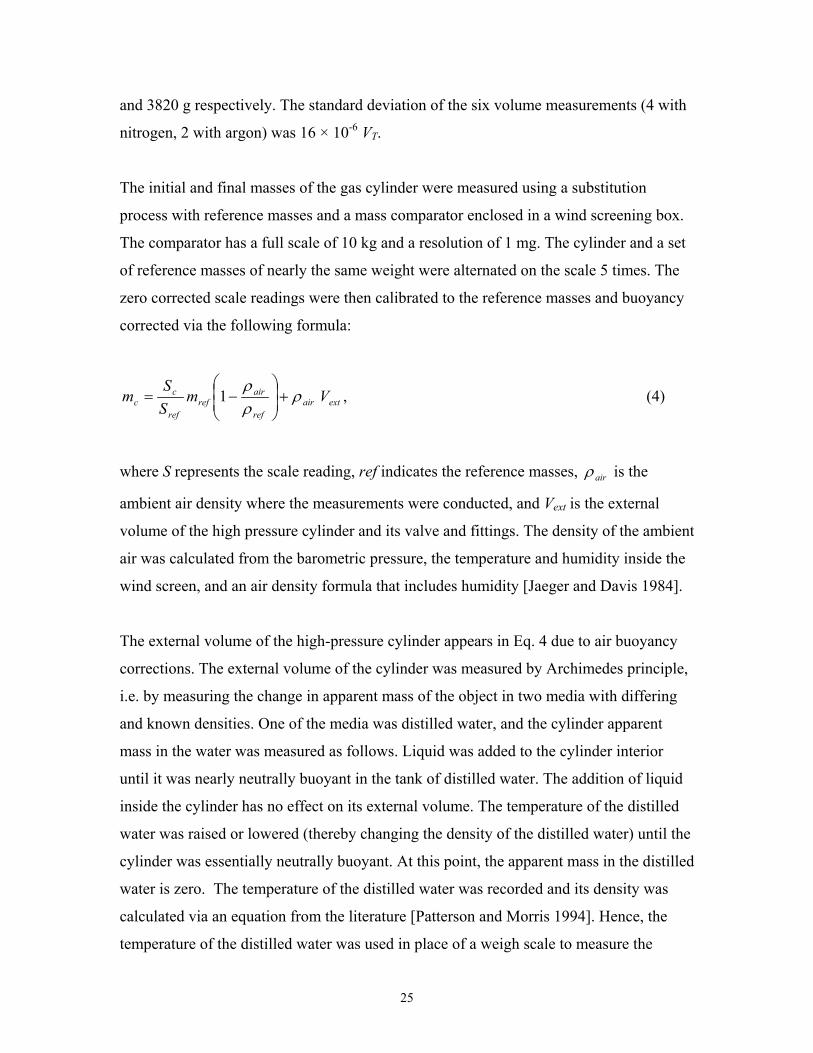
The initial and final masses of the gas cylinder were measured using a substitution

process with reference masses and a mass comparator enclosed in a wind screening box.

The comparator has a full scale of 10 kg and a resolution of 1 mg. The cylinder and a set

of reference masses of nearly the same weight were alternated on the scale 5 times. The

zero corrected scale readings were then calibrated to the reference masses and buoyancy

corrected via the following formula:

extairref

airref

ref

cc Vm

SS

m ρρρ

+

−= 1 , (4)

where S represents the scale reading, ref indicates the reference masses, airρ is the

ambient air density where the measurements were conducted, and Vext is the external

volume of the high pressure cylinder and its valve and fittings. The density of the ambient

air was calculated from the barometric pressure, the temperature and humidity inside the

wind screen, and an air density formula that includes humidity [Jaeger and Davis 1984].

The external volume of the high-pressure cylinder appears in Eq. 4 due to air buoyancy

corrections. The external volume of the cylinder was measured by Archimedes principle,

i.e. by measuring the change in apparent mass of the object in two media with differing

and known densities. One of the media was distilled water, and the cylinder apparent

mass in the water was measured as follows. Liquid was added to the cylinder interior

until it was nearly neutrally buoyant in the tank of distilled water. The addition of liquid

inside the cylinder has no effect on its external volume. The temperature of the distilled

water was raised or lowered (thereby changing the density of the distilled water) until the

cylinder was essentially neutrally buoyant. At this point, the apparent mass in the distilled

water is zero. The temperature of the distilled water was recorded and its density was

calculated via an equation from the literature [Patterson and Morris 1994]. Hence, the

temperature of the distilled water was used in place of a weigh scale to measure the

25

apparent mass in water. The apparent mass of the cylinder in air (with the liquid still

inside) was measured using the comparator described above. The density of air with

humidity was calculated as previously described. The external volume of the cylinder

was calculated for the nominal room temperature (Tref) of 296.5 K with the following

formula:

( ) ( )[ ] ([ )]refairairrefwaterwater

Awater

Aair

refext TTTTmm

TV−+−−+

−=

αραρ 3131, (5)

where the superscript A indicates apparent mass and α is the coefficient of linear thermal

expansion for the aluminum tank. The terms containing α correct for changes in the

cylinder volume due to differences between the water temperature, the air temperature,

and the reference temperature. However, for this particular case, these thermal expansion

issues could have been neglected since both the water temperature and air temperature

never differed from Tref by more than 1.5 K. The thermal expansion corrections to the

external volume were less than 0.5 cm3 or 100 × 10-6 Vext and the external volume has a

small sensitivity coefficient in the collection tank volume determination process.

The expansion of the external cylinder volume as a function of its internal pressure was

not negligible. The Archimedes principle measurements showed a volume increase from

4697.5 cm3 to 4709 cm3 between the 100 kPa and 12.5 Mpa pressures. This change

agreed well with predictions based on material properties, and the appropriate

experimental values for external volume were used in the cylinder mass calculations (Eq.

4), depending on whether the cylinder was empty or full. If this issue were neglected, it

would lead to relative errors in the mass change measurements of about 35 × 10-6.

26

5.3.2 Volume Expansion Method

The 34 L collection tank volume, the inventory volume for the large collection tank, and

the small inventory volume were all determined with a volume expansion method. In this

method, a known volume is pressurized, the unknown volume is evacuated, a valve is

opened between the two volumes, and the density changes within the two volumes are

used to calculate the unknown volume. Applying conservation of mass to the system of

the two tanks yields:

( )( ) extraV

VV −

−

−=

f2

i2

1i1

f1

2ρρρρ

, (6)

where the subscripts 1 and 2 refer to the known and unknown volumes respectively. As

before, the density values are based on pressure and temperature measurements of the gas

within the volumes and gas purity issues must be considered. Note that in many cases the

final densities can be considered the same in both volumes 1 and 2, but for the

determination of the 34 L tank volume, elevation differences between the two tanks

required a head correction to the pressure measurements and therefore the two densities

were not strictly equal. The difference in elevation resulted in a relative difference in gas

density of 20 × 10-6 even though the two tanks were connected.

6 Uncertainty Analysis of the 34 L and 677 L PVTt Flow Standards

In this section, we will analyze the uncertainty of the 34 L and 677 L PVTt standards. We

will begin by giving an overview of the subject of uncertainty analysis including the issue

of correlated uncertainties. Next we will give the results of the uncertainty analysis for

mass flow. In following sections, we will give uncertainties of the sub-components that

were combined to obtain the mass flow uncertainty. The largest source of uncertainty in

the flow measurement is drift of the pressure sensor over time, which contributes a

27

relative standard uncertainty of 60 × 10-6 to the determinations of the volumes of the

collection tanks and to the flow measurements.

6.1 Techniques for Uncertainty Analysis

The uncertainty of a mass flow measurement made with the PVTt standard use the

propagation of uncertainties techniques described in the ISO Guide to the Expression of

Uncertainty in Measurement [ISO 1996]. The process identifies the equations involved

in the flow measurement so that the sensitivity of the final result to uncertainties in the

input quantities can be evaluated. The uncertainty of each of the input quantities is

determined, weighted by its sensitivity, and combined with the other uncertainty

components to arrive at a combined uncertainty.

As described in the references [ISO 1996, Coleman and Steele 1999], consider a process

that has an output, y, based on N input quantities, xi. For the generic basis equation:

),,,( 21 Nxxxyy K= , (7)

if all the uncertainty components are uncorrelated, the standard uncertainties are

combined by root-sum-square (RSS):

( ) ( )∑=

∂∂

=N

ii

ic xu

xyyu

1

22

, (8)

where u(xi) is the standard uncertainty for each of the inputs, and uc(y) is the combined

standard uncertainty of the measurand. The partial derivatives in Eq. 8 represent the

sensitivity of the measurand to the uncertainty of each input quantity.

In cases where correlated uncertainties are significant (as in the following analysis), the

following expression should be used instead of Eq. 8:

28

( ) ( ) ( ) ( ) ( )∑ ∑ ∑=

−

= += ∂∂

∂∂

+

∂∂

=N

i

N

i

N

ijjiji

jii

ic xxrxuxu

xy

xyxu

xyyu

1

1

1 1

22

,2 , (9)

where r(xi, xj) is the correlation coefficient, ranging from –1 to 1, and equaling zero if the

two components are uncorrelated. As will be seen in the following analysis, some

uncertainty components in the present system are correlated and this leads to a significant

improvement in the uncertainty of the measurand.

A simple example of a correlated uncertainty is illustrative. Suppose that a thermometer

was used to measure a temperature difference. Also suppose that the only uncertainty in

the thermometer measurement was an unknown offset in its calibration. When the

difference between two temperatures was calculated from measurements made with this

thermometer, the offset would cancel and would not contribute to the uncertainty of the

temperature difference. In this case, the subtraction process used to calculate the

difference leads to sensitivity coefficients of opposite sign for the two temperature

measurements. Since the sensor always has the same offset, the uncertainties are perfectly

correlated (r(xi, xj) = 1). When this hypothetical scenario is processed through Eq. 9, the

uncertainty of the temperature difference is zero. Of course in a real case, there would be

other, uncorrelated uncertainties that would make the uncertainty of the temperature

difference non-zero. Nonetheless, the example demonstrates that under certain

circumstances, correlated uncertainties will reduce the uncertainty of a measured

quantity.

In the following uncertainty analysis, correlated and uncorrelated uncertainties will be

treated as separate components, even if they are related to the same physical quantity. For

instance, there will be a correlated as well as an uncorrelated inventory pressure

component. In this manner, the correlated components can be considered as having a

correlation coefficient of 1, while uncorrelated components have correlation coefficients

of 0. This approach simplifies the process to deciding which uncertainty sources are

correlated versus uncorrelated and checking that the assumption of perfect correlation is

reasonable.

29

Most of the equations utilized to calculate flow, mass, volume, and other necessary

intermediate quantities for the PVTt standard have been discussed in prior sections. In

Fig. 10 the information is summarized in a diagram that shows the measurement chain

used to calculate flow. At the top of the diagram is the output, mass flow. At the second

level are the inputs to Eq. 2, the quantities needed to calculate mass flow: density,

volumes, and collection time. To calculate density, the inputs to the equation of state are

necessary: pressure, temperature, compressibility, the universal gas constant, and

molecular weight. The other necessary quantities and their basis equations are shown as

well. Figure 10 will serve as a guide for the PVTt uncertainty analysis.

Eq. 6

Eq. 5

Eq. 2

Eq. 4

Eq. 3

m&

IV

xρTV

t∆

P

T

Zm

refmextV

airρ

waterρ

R

xρ

M

airρm

Figure 10. The chain of measurements and equations used for the PVTt flow standard.

30

The discharge coefficient resulting from a flowmeter calibration will have additional

uncertainties not considered herein due to measurements associated with the meter under

test. For instance, if the meter under test is a critical flow venturi, uncertainties related to

the temperature and pressure measurements at the meter must be included in the

uncertainty of the discharge coefficient.

The uncertainties tabulated herein are k = 1, standard, or 68 % confidence level

uncertainties. At the conclusion of the uncertainty analysis, a coverage factor of 2 will be

applied to give an expanded uncertainty for mass flow measurements with an

approximate 95 % confidence level. In the remainder of this section, we will give the

uncertainty of mass flow for both the 34 L and 677 L PVTt systems, and then the

uncertainty components that contribute to the PVTt mass flow measurement will be

traced to their fundamental sources.

6.2 Mass Flow Uncertainty

Table 2. Uncertainty of nitrogen flow measurement with the 677 L standard.

Uncertainty Category Standard Uncertainty

(k = 1)

Contrib Comments

Flow (677 L, N2) Relative (×106) (%)

Tank volume 71 48.44 cm3 50 to 23 see Table 15

Tank initial density 10 2.27 × 10-12 g/cm3 1 to 0

Tank final density 68 7.77 × 10-8 g/cm3 45 to 21 see Table 9

Inventory mass change 0 to 109 0.084 g 0 to 53 see Table 21

Collection time 15 0.287 ms 0 to 1 see Table 11

Std deviation of repeated meas. 20 0.001 g/sec 4 to 2

RSS (combined uncertainty) 102 to 150

Expanded uncertainty (k = 2) 204 to 300

The uncertainty for flows between 20 L/min and 2000 L/min of nitrogen or argon in the

677 L tank is given in Table 2. The standard uncertainty of each sub-component is given

31

in both relative (× 10-6) and dimensional forms. The units of the dimensional values are

given in the third column. The relative contribution of each sub-component to the

combined uncertainty is listed in the fourth column. This contribution is the percentage of

the squared individual component relative to the sum of the squares of all sub-

components. The uncertainty from the inventory volume, the combined uncertainty, the

expanded uncertainty, and the uncertainty contributions are given as a range covering the

minimum to maximum flow. To calculate their relative uncertainty in Table 2, the tank

initial density was normalized by the tank final density and the inventory mass change

was normalized by the total mass collected.

At the highest flow, uncertainty contributions are principally divided between the tank

volume, the final gas density, and the inventory uncertainty. The k = 2 uncertainty falls to

204 × 10-6 for the smallest flows as the uncertainty contributions of the inventory

volume become negligible. For an air flow measurement, the uncertainty of the 677 L

system is less than 500 × 10

m&

-6 over the entire flow range and the uncertainty is driven

by the tank final density measurement (80 % contributor).

m&

Table 3. Uncertainty of nitrogen flow measurement with the 34 L standard.

Uncertainty Category Standard Uncertainty

(k = 1)

Contrib Comments

Flow (34 L, N2) Relative (×106) (%)

Tank volume 116 3.955 cm3 72 to 28 see Table 16

Tank initial density 10 2.27 × 10-12 g/cm3 1 to 0

Tank final density 68 7.77 × 10-8 g/cm3 25 to 10 see Table 9

Inventory mass change 0 to 170 0.007 g 0 to 61 see Table 22

Collection time 15 0.287 ms 0 to 0 see Table 11

Std deviation of repeated meas. 20 4 × 10-5 g/sec 2 to 1

RSS (combined uncertainty) 137 to 219

Expanded uncertainty (k = 2) 274 to 438

32

Table 3 presents the uncertainty of flow measurements from the 34 L system for flows

between 1 L/min and 100 L/min. The expanded uncertainty varies between 270 × 10-6

and 440 × 10

m&-6 . At high flows, the significant uncertainty sources are the tank volume,

the tank final density, and the uncorrelated inventory uncertainties. For low flows, the

major contributors are tank volume and final gas density. For air flow measurements, the

34 L system has a nearly constant uncertainty over its entire flow range of about

500 × 10

m&

-6 and it is driven by the uncertainty of the final gas density. m&

6.3 Pressure

A Ruska Model 2465-754 gas lubricated piston pressure gauge is used as the primary

pressure standard to calibrate pressure transducers within the Fluid Flow Group. The

uncertainties in a single pressure measurement made with this device are listed in Table

4. Uncertainties in the pressure standard can be traced to the effective area of the piston,

piston thermal expansion, the masses, local gravity, and the measurement of the pressure

under the bell jar covering the piston and masses (necessary for absolute pressure

measurements). The uncertainty shown in Table 4 is for a pressure value of 100 kPa. No

buoyancy corrections are made to the masses since the reference pressure, and hence the

density under the bell, are small enough that the buoyancy corrections (and uncertainties)

are negligible (<<1 × 10-6 P). The uncertainty of the piston pressure gauge is 17 × 10-6 P

at 100 kPa.

33

Table 4. Uncertainties for a 100 kPa pressure measurement made with the piston pressure

gage used as the standard for pressure calibrations.

Uncertainty Category Standard Uncertainty

(k = 1)

Contrib Comments

Relative (×106) (kPa) (%)

Piston Pressure Gage

Pressure value 100

piston effective area 12 0.0012 59 from NIST Pressure and Vacuum Group cal.

thermal expansion 6 0.0006 15 assume T unc of 0.2K

masses 1 0.0001 0 Mass Group calibration

local gravity 0.2 0.00002 0 9.801011+/- 0.000002

air density for buoyancy 0 0 0 neg. air density relative to mass density

ref. P for absolute 10 0.001 41 based on calibration data of the vac gauge

RSS 17 0.0017

6.3.1 Collection Tank Pressure

Measurements of the collection tank initial pressure are made with a pair of thermocouple

vacuum gauges (Varian Convectorr P-type) that have been calibrated by comparison to a

reference standard in the NIST Pressure and Vacuum Group. The manufacturer’s

uncertainty specification for this gauge is 10 % of reading. Based on the NIST calibration

results, the consistent agreement between the redundant sensors, and the repeatable

readings of the gauges at the vacuum pump ultimate pressure, a standard uncertainty of

5 % of reading will be used. As will be seen when the components are combined to give

the flow measurement uncertainty, this large value has little impact due to the low initial

pressure in the collection tank (20 Pa).

Pressure measurements of the full collection tank are made with a Paroscientific Model

740 with a full scale of 200 kPa. The manufacturer’s uncertainty specification for this

transducer is 0.01 % of full scale, but under the conditions of the present usage, the

uncertainty is less. The uncertainties in the collection tank pressure measurement are

34

listed in Table 5. They include the uncertainties from the piston pressure gage, the long

term drift of the Paroscientific transducer which has been quantified by periodic re-

calibrations, as well as the residuals from the best fit calibration equation (including

hysteresis), and thermal effects. Uncertainties due to spatial non-uniformity of pressure

within the tank and time response of the sensor are negligible since the calibration

procedure is to wait as much as 20 minutes for equilibration before the measurements are

made.

Figure 11 is a control chart that shows the changes in pressure calibration versus time at a

pressure of 100 kPa for one of the pressure transducers used to measure collection tank

pressure. Also shown are the k = 1 uncertainty tolerance bounds (64 × 10-6 P from Table

5) and error bars that represent the k = 1 uncertainty of the piston pressure gauge used to

calibrate the sensor (17 × 10-6 P from Table 4).

-150.0

-100.0

-50.0

0.0

50.0

100.0

150.0

1/1/99 1/1/00 12/31/00 12/31/01 12/31/02 12/31/03

Date

(P-P

last

) / P

* 1

06

Newsensor

Figure 11. A calibration control chart for a 200 kPa pressure transducer used to measure

the collection tank pressure.

Temperature effects as large as 40 × 10-6 P have been observed in the tank pressure

sensor, and care was taken to minimize their influence. When the tank is quickly filled

from a pressurized cylinder during the volume determination process, cold gas enters the

sensor, cooling it. The pressure readings asymptotically approach a final value as the

35

sensor returns to room temperature (with a time constant of approximately 1 hr). The

temperature dependence of the sensor was confirmed by testing with an environmental

chamber. Temperature effects also result in a hysteresis loop for the sensor calibration

data that enlarges the calibration fit residuals. The calibration process entails increasing

and decreasing the pressure in steps. The pressure steps result in heating and cooling of

the pressure sensing elements and a hysteresis loop. Therefore the residuals of the

pressure calibration fit include contributions due to thermal effects. We noticed that the

thermal effects due to pressure changes in the transducers can be larger than the values

given in Table 5. During volume determinations, we allowed sufficient time for the

sensor to return to room temperature so that the remaining temperature effects were much

smaller than the allowance for calibration drift.

Table 5. Uncertainties in the collection tank pressure measurement at 100 kPa.

Uncertainty Category Standard Uncertainty

(k=1)

Contrib Comments

Relative (×106) (kPa) (%)

Pressure Measurement

Pressure value 100

piston pressure gage 17 0.0017 7 from Table 4

drift 60 0.0060 88 < 0.01 % in 6 mos, assume rect.

residuals, hysteresis, thermal effects 14 0.0014 5 from cal. records, experiments

RSS 64 0.0064

6.4 Temperature

The temperature sensors used in the flow standard are traceable to the NIST

Thermometry Group through calibrations made with a four-wire thermister transfer

standard (Thermometrics Model TS8901) and a recirculating water constant temperature

bath. The uncertainty of the transfer standard thermister is 1.2 mK (see Table 6). The drift

of the transfer standard is considered negligible based on 7 annual calibrations that have

always differed from each other by less than the calibration uncertainty.

36

Table 6. Uncertainties for the Fluid Flow Group temperature transfer standard.

Uncertainty Category Standard Uncertainty

(k =1)

Contrib Comments

Relative (×106) (mK) (%)

Temperature Transfer Standard

Temperature value 3 × 105

Thermometry Group cal 4 1.2 94 unc. for 274 K to 368 K

fit residuals 1 0.3 6 some years, 1/6 this size

drift 0 0 0 less than discernable given cal unc.

radiation, self-heating, etc. 0 0 0 deeply immersed in water bath

RSS 4 1.2

6.4.1 Collection Tank Temperature

The measurement of the temperature of the gas in the collection tank has additional

uncertainties that are listed and quantified in Table 7. Temperature is measured with YSI

Model 46000 thermisters in 3 mm diameter stainless steel sheaths, a Keithley model 224

current source, a Keithley model 7001 switch system, and a Keithley model 2002

multimeter. Uncertainty sources include the temperature transfer standard covered by

Table 6, the uniformity and stability of the water bath used to calibrate the thermisters,

and the residuals of the best-fit equation to the calibration data. The largest uncertainty

component is the calibration drift between periodic calibrations. Radiation and stem

conduction are negligible since the thermisters are immersed at least 15 cm in room

temperature water. Tests were conducted to measure the significance of self-heating by

varying the thermister current while the sensor was held in a stable water bath and

watching the resulting change in sensor reading. Based on this experiment, the current

through the 5000 ohm thermisters was set to 10 µA which leads to self-heating of less

than 1 mK. The PVTt bath stability and uniformity (1 mK) were discussed earlier, as was

the issue of thermal equilibrium between the water bath and the gas in the collection tank.

The sensors are calibrated over their entire range of usage, so there is no uncertainty

37

related to extrapolation of their calibration data. Uncertainty related to the time response

of the thermisters is negligible since the time constant for the sensor is on the order of

10 s and the wait for thermal equilibrium is 30 or more times longer.

Small portions of the gas collection tank are not immersed in the water bath. They

include the tubing connecting the outlet of the diverter valve to the collection tank, the

tubing that connects the tank to pressure and vacuum transducers, and the internal volume

of these transducers. Because we assumed that the bath temperature represents the gas

temperature, and the room temperature may differ from that of the bath, the small portion

of the tank not immersed leads to a gas temperature uncertainty. The room temperature is

maintained at 23.5 ± 1°C. The fractional error in mass contained in the collection tank

due to a 1 K difference between the room and the water bath is:

TT

VV

mm

T

out δδ≈ , (10)

where Vout is the volume of the portion of the tank that is at room temperature and Tδ is

the difference between the room and water bath temperatures. For the large tank, Vout is

200 cm3 and the total tank volume is 677 L. For Tδ of 1 K, the relative mass uncertainty

is 1 × 10-6. This uncertainty will be treated as an uncertainty in the average gas

temperature of 1 × 10-6 T or 0.3 mK in the following analysis. For the small tank this

temperature uncertainty is 1.2 mK or 4 × 10-6 T.

By RSS of the components listed in Table 7, the combined uncertainty for the average

temperature of the gas in the collection tank is 7 mK when using the thermisters

dedicated to the flow standard.

38

Table 7. Uncertainty of average gas temperature in the collection tank with the dedicated

temperature sensors.

Uncertainty Category Standard Uncertainty

(k =1)

Contrib Comments

Relative (×106) (mK) (%)

Tank Gas Average Temperature

Temperature value 297000

temperature transfer standard 4 1.2 4 from Table 7

cal. bath uniformity and stability 3 1 2 based on notes made during cal

fit residuals 7 2 9

drift (I, R, DMM, thermistors) 20 5.8 77 YSI spec is <10mK/10 mo., assume rect.

radiation, stem cond., self-heating 3 1 2 expt. varied current, 5 mK, assume rect.

PVTt bath uniformity and stability 3 1 2 based on experimental measurements

diff. between water and room T's 4 1.2 3 see Eq. 10

extrapolation 0 0 0 cal covers whole operating range

sensor time constant 0 0 0 wait time is >10 × sensor time constant

RSS 22 7

6.5 Compressibility, Molecular Weight, and Gas Constant

The remaining contributors to gas density uncertainty are the compressibility, the

molecular weight, and the gas constant. Four gas cases will be considered. Tank volume

determinations were conducted with ultra high purity nitrogen (99.999 %) and ultra high

purity argon (99.999 %). During normal calibrations, industrial liquid nitrogen vaporized

from dewars (99.998 %) and compressed, dried air are used.

6.5.1 Gas Constant

The universal gas constant is known with relative standard uncertainty better than

2 × 10-6 [Moldover et al. 1988].

39

6.5.2 Compressibility

The compressibility factor can be calculated from the following expression:

21 nn CBZ ρρ ++= , (11)

where nρ is the molar density (mol/ cm3) and B and C are the second and third virial

coefficients respectively. For nitrogen, the virial coefficients can be calculated from the

correlations:

24

2 10636.765125.021.131 TTBN−×−++−= , (12)

2

2 015.035.112.3454 TTCN +−= , (13)

where temperature is in K and B and C are in cm3/mol and cm6/mol2 respectively and the

units of the constants have been surpressed. For dry air the correlations for the virial

coefficients are:

2410833.766785.006.137 TTBAir

−×−++−= , (14)

2016.040.129.3528 TTCAir +−= . (15)

These expressions are the result of least squares best fitting to outputs from a database of

the property measurements by numerous experimenters [Lemmon et al. 2002]. Equations

12 through 15 were fitted to data over the range of 270 K to 330 K. This range allows

application of the correlations at the conditions found in the test section of the flow

standard. However, it should be noted that the conditions in the collection tank are much

narrower, with pressures ranging from 0 kPa to 101 kPa at a nearly constant temperature

of 296.5 K. For these narrower conditions, the third virial coefficient could be ignored

with negligible impact on the density uncertainty.

40

Uncertainty estimates for experimental studies of compressibility are often unavailable,

especially for older publications. Comparison of previously compiled compressibility

values obtained by various researchers [Dymond and Smith 1980, Hilsenrath et al. 1955,

Span et al. 2000, Lemmon et al. 2000] shows agreement to within 10 × 10-6 in the 270 K

to 330 K temperature range at 100 kPa. Perhaps more valuable is that this level of

agreement is achieved between compressibility measurements made by the traditional

PVT method and by the more recent speed of sound techniques [Trusler et al. 1997].

Based on this information, a relative standard uncertainty of 10 × 10-6 will be used for the

experimental measurements of compressibility. This uncertainty is for a pressure of

100 kPa and it scales with density. The residuals of the equation fitting process to the

experimental data are negligibly small (<1 × 10-6 Z). The uncertainty components of the

compressibility factor are listed in Table 8.

Table 8. Uncertainty of the compressibility for nitrogen, argon, and dry air. Uncertainty Category Standard Uncertainty

(k =1)

Contrib Comments

Compressibility (Z) Relative (×106) (-) (%)

Compressibility value 1

experimental data 10 1 × 10-5 99 based on analysis of literature

impurity effects on Z 1 1 × 10-6 1

residuals of best fit 0 0 0 <1 × 10-6

RSS 10 1 × 10-5

The source of the dry air used in the flow standard is a Joy oil-free two stage

reciprocating compressor and a Zurn refrigeration dryer. The mole fraction of water in

this air source is 0.0010 ± 0.0005. This uncertainty in composition leads to uncertainty in

the compressibility of only 1 × 10-6 Z. The uncertainty in compressibility due to

impurities is smaller for the other gases.

41

6.5.3 Molecular Weight

The departure of the molecular weight of ultra high purity nitrogen, industrial liquid

nitrogen, and ultra high purity argon from the molecular weight of the pure substance was

examined using the impurity specifications of the gas manufacturer. This analysis results

in molecular weight relative standard uncertainties less than 1 × 10-6, but 1 × 10-6 will be

assumed for the molecular weight of nitrogen (28.01348 g/mol) and argon

(39.94800 g/mole). For the dry air described above, the molecular weight is

28.9532 g/mol and its relative standard uncertainty is 190 × 10-6 due to the variability of

water content.

6.6 Density

Now that the sub-components have been quantified, the uncertainty of density

measurements made in the collection tank with nitrogen and argon (for volume

determinations and for flow measurements) and with dry air (for flow measurements) can

be calculated and they are presented in Tables 9 and 10. For the pure gases, the relative

standard uncertainty is 68 × 10-6 and the primary contributor is the pressure measurement.

For air, the relative standard uncertainty is 208 × 10-6 and the largest contribution is due

to water content variations. The uncertainties of the density of ambient air (needed for

buoyancy corrections) and of distilled water are considered in the section pertaining to

tank volume determinations.

42

Table 9. The uncertainty of collection tank gas density for nitrogen and argon.

Uncertainty Category Standard Uncertainty

(k=1)

Contrib Comments

Collection Tank Density (N2 & Ar) Relative (×106) (%)

pressure 64 6.45 × 10-3 kPa 88 from Table 5

temperature 22 6.47 mK 10 from Table 7

compressibility 10 1 × 10-5 2 from Table 8

molecular weight (purity) 1 2.80 × 10-5 g/mol 0

gas constant 2 1.41 × 10-2 (cm2)/(s2K) 0

RSS 68 7.82 × 10-8 g/cm3

Table 10. The uncertainty of collection tank gas density for dry air from the NIST Fluid

Flow Group small compressor and dryer system.

Uncertainty Category Standard Uncertainty

(k =1)

Contrib Comments

Collection Tank Density (Air) Relative (×106) (%)

pressure 64 6.45 × 10-3 kPa 9 from Table 5

temperature 22 6.47 mK 1 from Table 7

compressibility 10 1 × 10-5 0 from Table 8

molecular weight (purity) 190 5.5 × 10-3 g/mol 89

gas constant 2 1.41 × 10-2 (cm2)/(s2K) 0

RSS 208 2.38 × 10-7 g/cm3

6.7 Collection Time

As explained in section 5.2.3, the collection time is an approximate time measured by

timers that is then corrected via analysis of records of the inventory pressure data and

trigger voltages to minimize inventory mass and improve uncertainty cancellation. The

base time is measured redundantly with two Hewlett-Packard Model 53131A counters.

The counter calibration and usage leads to less than 0.01 ms uncertainty. Due to the

3000 Hz recording frequency of the inventory pressure and trigger data, the actual rise of

43

the trigger voltage can be any time within a 0.33 ms window. Assuming a rectangular

distribution, the post-processing corrections will have a standard uncertainty of 0.19 ms.

This uncertainty applies to both the start and stop times. The time uncertainties of the two

pressure measurements used in the mass cancellation procedure are negligible since the

times are found by interpolation of the data records and are much smaller than 0.33 ms.

The combined collection time uncertainty is 0.3 ms (see Table 11).

Table 11. Collection time uncertainties.

Uncertainty Category Standard Uncertainty

(k =1)

Contrib Comments

Relative (×106) (ms) (%)

Collection Time

Time value 100000

timer cal and usage 0 0.01 0 base time uncertainty

inventory correction (start) 2 0.19 50 3000 Hz, rectangular distribution

inventory correction (stop) 2 0.19 50 3000 Hz, rectangular distribution

RSS 3 0.3

6.8 Volume of the 677 Liter Collection Tank (Gravimetric Method)

The uncertainty of the determination of the collection tank volume by the previously

described gravimetric method (section 5.3.1) is traceable to the uncertainty of the mass

and density measurements made during the process, which are in turn dependent on the

quantities shown in Fig. 10. The uncertainty of the density measurements for the pure

nitrogen and argon gases used for the volume measurements was given in Table 9. The

scale used was a Mettler-Toledo model PR10003, which has a 10 kg capacity. The

uncertainty of the mass measurements of the high-pressure cylinder before and after

discharge is dependent on the buoyancy corrections (ambient air density and cylinder

external volume), the reference masses used with the mass comparator, and the

performance of the mass comparator. The measurement of the external volume of the

high-pressure cylinder via the Archimedes principle was described in an earlier section.

44

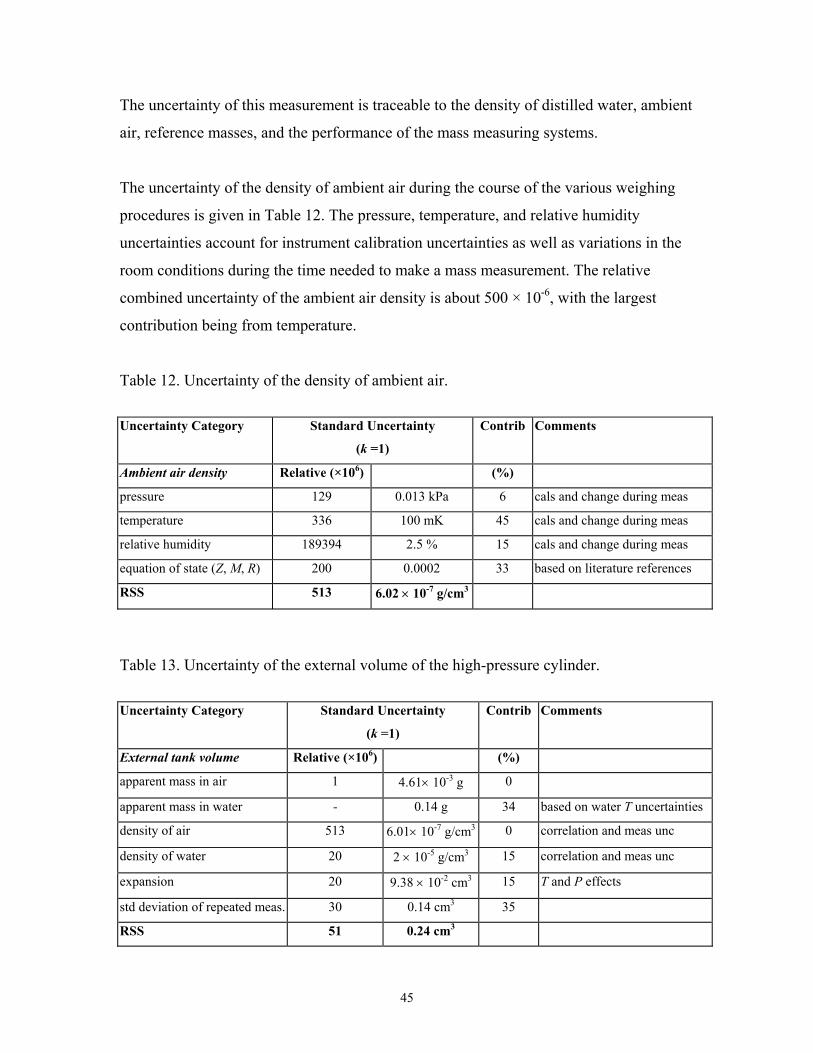
The uncertainty of this measurement is traceable to the density of distilled water, ambient

air, reference masses, and the performance of the mass measuring systems.

The uncertainty of the density of ambient air during the course of the various weighing

procedures is given in Table 12. The pressure, temperature, and relative humidity

uncertainties account for instrument calibration uncertainties as well as variations in the

room conditions during the time needed to make a mass measurement. The relative

combined uncertainty of the ambient air density is about 500 × 10-6, with the largest

contribution being from temperature.

Table 12. Uncertainty of the density of ambient air.

Uncertainty Category Standard Uncertainty

(k =1)

Contrib Comments

Ambient air density Relative (×106) (%)

pressure 129 0.013 kPa 6 cals and change during meas

temperature 336 100 mK 45 cals and change during meas

relative humidity 189394 2.5 % 15 cals and change during meas

equation of state (Z, M, R) 200 0.0002 33 based on literature references

RSS 513 6.02 × 10-7 g/cm3

Table 13. Uncertainty of the external volume of the high-pressure cylinder.

Uncertainty Category Standard Uncertainty

(k =1)

Contrib Comments

External tank volume Relative (×106) (%)

apparent mass in air 1 4.61× 10-3 g 0

apparent mass in water - 0.14 g 34 based on water T uncertainties

density of air 513 6.01× 10-7 g/cm3 0 correlation and meas unc

density of water 20 2 × 10-5 g/cm3 15 correlation and meas unc

expansion 20 9.38 × 10-2 cm3 15 T and P effects

std deviation of repeated meas. 30 0.14 cm3 35

RSS 51 0.24 cm3

45

The uncertainties related to the determination of the external volume of the high-pressure

cylinder are listed in Table 13. The 1 × 10-6 relative standard uncertainty for the apparent

mass in air is based on uncertainty calculations for the true mass of the weighed cylinder

(discussed later). The uncertainty of the apparent mass in water is based on the recorded

temperatures of water that made the cylinder barely sink or barely float. Uncertainty of

the water temperature for neutral buoyancy of 0.2 K leads to a value for the uncertainty

of the apparent mass in water. This uncertainty is not reported in a relative form since the

apparent mass in water is zero and the relative uncertainty is therefore undefined. The

RSS is calculated using the results in the third column and their sensitivity coefficient.

The water density uncertainty includes thermometer uncertainties, estimates of non-

uniformity of the water temperature, and uncertainty of the water density correlation

obtained from the literature. As previously stated, different values of external volume

were used for the full and empty cylinder due to pressure dilation, but an uncertainty

related to pressure and temperature effects is included here. The collection tank volume is

not very sensitive to this external tank volume, hence larger uncertainty values than

51 × 10-6 Vext could certainly be tolerated.

Table 14. Uncertainty of the high-pressure cylinder mass measurement.

Uncertainty Category Standard Uncertainty

(k =1)

Contrib Comments

Final mass of high P cylinder Relative (×106) (%)

reference masses 0.5 1.91 × 10-3 g 26 from NIST Mass Group cal report

room air density 513 6.01 × 10-7 g/cm3 45

reference mass density 0 0 g/cm3 0 same value for cal. and usage

external cylinder volume 51 0.24 cm3 1 from unc. of Archimedes method

std deviation of repeated meas. 1 0.002 g 28

RSS 1 0.00376 g

46

The relative standard uncertainties of the cylinder mass measurement (Table 14) are quite

small (1 × 10-6) with the major components being the reference masses, the room air

density (for buoyancy corrections) and the performance of the comparator (repeatability

of the 5 measurements made with the comparator, a type A uncertainty). The complete

mass measurement process was repeated several times for the full and empty cylinder

conditions to assess the repeatability of the process, and these repeated mass values never

differed by more than 1 × 10-6 mc. This repetition was undertaken since a previously used

cylinder showed changes over time, probably due to absorption of water from room

humidity variations. The uncertainty of the density of the reference masses (7.8 g/cm3) is

negligible since the sensitivity of mass measurements to this component is extremely

small. While some of the mass measurement uncertainties for the full and empty cylinder

are correlated and this could be used to reduce the uncertainty of the mass delivered to

the collection tank, this benefit was not utilized since the improvement was not

significant. A table of uncertainty components of the empty cylinder mass measurement

is not presented because it is so similar to Table 14.

Finally, the uncertainty of the collection tank volume is presented in Table 15. The

relative value of the initial collection tank density uncertainty is quite large, but the

sensitivity of the result to this quantity is very small. Recall that uncertainty due to the

effects of room temperature variations on the portion of the collection tank not

submerged has already been incorporated as a temperature uncertainty. The effects of

pressure changes from vacuum to 100 kPa on the tank volume have been considered

analytically and found to be negligible. A small volume (1 cm3) of connecting tubing and

valve was necessary to introduce gas from the pressurized cylinder to the collection tank.

This volume was measured with alcohol and a graduated syringe and the uncertainty of

this volume correction was estimated to be 0.5 cm3. By far the largest contribution is

from the final gas density, and this in turn is nearly completely traceable to the pressure

measurement.

47

Table 15. Uncertainty of the 677 liter collection tank volume.

Uncertainty Category Standard Uncertainty

(k =1)

Contrib Comments

Collection tank volume Relative (×106) (%)

Initial mass of high P cylinder 1 0.00385 g 2 see Table 14

Final mass of high P cylinder 1 0.00376 g 2 see Table 14

initial collection tank gas density 100000 1.14 × 10-9 g/cm3 0

final collection tank gas density 68 4.25 × 10-8 g/cm3 92 see Table 9

expansion due to P and T 0 0 cm3 0 < 1 ppm

extra volume uncertainty 1 0.50 cm3 0 related to liq transfer meas.

std deviation of repeated meas. 16 10.85 cm3 5 6 measurements, 2 gases

RSS 71 48.44 cm3

Each gravimetric volume determination required one day to complete due to the time

required to achieve ultimate vacuum in the tank (1 Pa), the time for the pressure

transducer to reach thermal equilibrium after filling, and the time to take multiple

cylinder mass measurements separated by an hour each time. The volume measurements

were done 6 times, 4 times with nitrogen and twice with argon. The standard deviation of

these six determinations was 16 × 10-6 VT, quite good when one considers that two

different gases were used and the uncertainty of their equations of state. The combined

uncertainty of the 677 L collection tank volume is 71 × 10-6 VT. The 677 L volume was

used as a reference to determine the remaining three unknown volumes via the volume

expansion method.

6.9 Volume of the 34 Liter Collection Tank (Volume Expansion Method)

As explained in section 5.3.2, the volume expansion method is performed by pressurizing

a known volume with pure gas and opening a valve to expand the gas into a previously

evacuated unknown volume. The density changes and known volume are used to

calculate the unknown volume via Eq. 6. In this case the 677 L volume was used to

determine the large inventory volume and the 34 L collection tank volume. Subsequently,

the 34 L collection tank volume was used to determine the small inventory volume.

48

Significant uncertainties of the volume expansion method are related to density and the

measurement of pressure. Many components of the previously given pressure uncertainty

are correlated for a pressure change measurement made with the same pressure

transducer over a short time period (about 1 h). Uncertainties of the piston pressure gauge

and the sensor drift can be considered correlated for the short time period and small

pressure changes involved (5 kPa to 8 kPa out of 200 kPa full scale).

The uncorrelated uncertainties in the measurement of pressure change are due to sensor

non-linearity, resolution, hysteresis, and thermal effects. In order to quantify these

uncertainties for the volume expansion method, the piston pressure gauge was used to

repeatedly provide a reference step change of 6 kPa to the pressure transducer. The

pressure change measured by the pressure transducer was compared to the pressure

change calculated from the pressure standard. Based on these experiments, the

uncertainty of the pressure difference measurement during the 34 L tank volume

determination is 0.3 Pa

Table 16. Uncertainty of the 34 L tank volume determined by the volume expansion

method.

Uncertainty Category Standard Uncertainty

(k =1)

Contrib Comments

Collection tank volume Relative (×106) (%)

677 L volume 71 48.4 cm3 38 from gravimetric determination

large inventory volume 1788 1.298 cm3 0 from volume expansion method

677 L density change 40 3.53 × 10-9 g/cm3 12 dominated by pressure

34 L density change 65 -1.12× 10-7 g/cm3 32 dominated by pressure

extra volume uncertainty 15 0.5 cm3 2 measured by liq transfer

std deviation of repeated meas. 46 1.58 cm3 16 13 volume determinations

RSS 116 4.0 cm3

49

The 34 L tank volume uncertainty is summarized in Table 16. The largest uncertainty

contributions are from the 677 L volume uncertainty, the density change in the 34 L

volume, and the standard deviation of the repeated volume measurements. The

uncertainty of the density change in the 677 L volume is dominated by uncertainty in the

measurement of the pressure change. 6.10 Inventory Volume

The mass change in the inventory volume is negligible since we used the mass

cancellation procedure. However, since there are imperfections in the procedure,

uncertainty components related to the inventory mass change cannot be neglected.

Fortunately, the most significant of these uncertainty components (due to sensor time

constants) are correlated between the start and stop diversions for the methods of

operation used in this flow standard. Other correlated inventory volume uncertainties

include the pressure and temperature sensor calibrations and the differences between

sensed and stagnation values of pressure and temperature. For instance, the inventory

temperature is measured incorrectly low by the same amount at both the start and stop

conditions due to slow sensor response time, so cancellation of temperature uncertainty

occurs. More precisely, the uncertainty of the mass change within the inventory volume

caused by the correlated pressure and temperature uncertainties can be expressed as:

( ) ( )

21

2

22

2

)()()(1)(1)(

−+

−=∆ i

IiI

iIf

IfI

fIi

IiI

fIf

I

II Tu

T

PTu

T

PPu

TPu

TZRMV

mu (16)

where in this equation, u(PI), u(TI), and u(∆mI) are the uncertainties of the inventory

pressure, the inventory temperature, and the inventory mass change during the collection,

respectively. Note that if the uncertainties and the initial and final conditions are equal

(i.e. , , T , and ), then the terms within

parentheses cancel, and the flow uncertainty related to the inventory volume is zero.

Equation 16 demonstrates the benefit of matching the initial and final inventory

conditions to optimize the cancellation of correlated uncertainties.

)()( fI

iI TuTu = )()( f

Ii

I PuPu = fiI IT= f

Ii

I PP =

50

Not all of the measurement uncertainties of the inventory volume are correlated. For

perfect inventory mass cancellation, the pressure and temperature measured at specific

locations in the inventory volume must exhibit perfect correlation with the pressures and

temperatures throughout the inventory volume. In this way, the sensor readings

“represent” the conditions throughout the volume and when the readings at the specific

locations match, the conditions throughout the inventory volume are matched.

Unfortunately, this representative relationship may not exist and there may be

inconsistencies between the pressure and temperature fields between the start and stop

diversions. These inconsistencies may originate from a change in the inventory wall

temperature or from differences in the flow paths between the start and stop diversions.

The spatial inconsistencies are uncorrelated and their magnitude is likely a function of the

mass flow.

Another source of inventory uncertainty, alluded to previously, is due to imperfection in

matching the stop diversion pressure to the start diversion pressure. Recall that the

inventory pressure is recorded while the bypass valve is open (nominally the barometric

pressure), and that the tank filling is stopped when the inventory pressure regains this

same pressure. In this way, the pressure at the beginning of the dead-end time transients

is nearly equal for both diversions and the symmetry of the transients is improved. At

high flows, it becomes more difficult to match these initial pressures in the high speed

data records and a “trigger pressure difference” that increases with increasing flow

occurs. The size of the trigger pressure difference can be reduced by using faster sensors

and a fast data acquisition and diverter valve control system. An example of the trigger

pressure difference can be seen in Fig. 7, where at times less than zero, the pressure

traces differ by about 1.6 kPa. The trigger pressure difference, coupled with the

“historical” nature of the inventory pressure measurements due to the sensor time

constant, is another reason that matching of the pressure sensor readings does not

necessarily lead to matching of the actual conditions in the inventory volume. Hence the

trigger pressure difference is another source of inventory uncertainty that scales with the

flow.

51

It is difficult to assess the magnitude of the uncorrelated uncertainties of pressure and

temperature between the start and stop diversions in the inventory volume. Our strategy is

to estimate the uncorrelated inventory uncertainties and then perform experiments (see

Section 7) to confirm that the estimates are reasonable. We assumed that the uncorrelated

inventory uncertainties scale with the flow and are essentially zero at the minimum flow

of each tank. We will assume values of 3 kPa and 9 K (about 3 % of the nominal values)

for the maximum flow of each tank.

Uncertainties related to the fast measurement of pressure with a 700 kPa full scale Heise

Model HPO sensor in the inventory volume are listed in Table 17, separated into

correlated and uncorrelated components.

Table 17. Uncertainties in the inventory pressure measurement, correlated and

uncorrelated, for maximum flow conditions.

Uncertainty Category Standard Uncertainty

(k =1)

Contrib Comments

Relative (×106) (kPa) (%)

Inventory Pressure Measurement

Pressure value 100

sensor calibration 3000 0.30 0

sensor time response 1350000 135 100 from inv. model at max flow

sensed vs. stagnation 710 0.071 0 for max flow

RSS (correlated) 1350004 135

sensor repeatability 3.00E+02 0.03 0 from calibration data

spatial inconsistency 3.00E+04 3 100 estimated

RSS (uncorrelated) 30001 3.0

Table 18. Inventory temperature uncertainties, correlated and uncorrelated, for the

maximum flow for each tank.

52

Uncertainty Category Standard Uncertainty

(k =1)

Contrib Comments

Relative (×106) (mK) (%)

Inventory Thermocouple

Temperature value 297000

sensor calibration 337 100 0

sensor time response 168350 50000 97 from inventory model

sensed vs. stagnation 50 15 0 for max flow

RSS (correlated) 168351 50000

sensor repeatability 286 85 0 from calibration data

spatial inconsistency 30303 9000 100 estimated

RSS (uncorrelated) 30304 9000

The uncertainties of the measurement of temperature in the inventory volume are listed in

Table 18, again divided into correlated and uncorrelated components. The uncertainties

include calibration, time response, sensed versus stagnation issues, sensor repeatability,

and spatial non-uniformity or inconsistency between start and stop diversions.

Table 19. Uncertainty of the 1000 cm3 (large) inventory volume.

Uncertainty Category Standard Uncertainty

(k =1)

Contrib Comments

Collection tank volume Relative (×106) (%)

677 L volume 71 48.4 cm3 0

677 L density change 1039 3.41× 10-9 g/cm3 54

inv. vol. density change 120 2.81× 10-7 g/cm3 1

extra volume uncertainty 526 0.5 cm3 14

std. deviation of repeated meas. 799 0.76 cm3 32

RSS 1419 1.35 cm3

The uncertainties for the large and small inventory volumes determined by the volume

expansion method are presented in Tables 19 and 20. Although the relative uncertainties

53

of these volumes are large, the sensitivity of the flow measurement to these volumes is

small due to the inventory mass cancellation scheme and the relatively small size of VI.

For the very small pressure changes used for the inventory volume determinations, the

ability of the pressure transducers to measure the pressure change becomes a large

uncertainty issue. The standard deviation of repeated measurements is large for these

volume determinations due to the uncertainty of the small pressure change measurements.

The ratio of the known tank volume to the unknown inventory volume is about 500 to 1,

hence the pressure change is only about 0.3 kPa for an initial pressure of 150 kPa. The

uncertainty of the pressure change measurement (0.3 Pa) is based on the previously

described experiments using the pressure standard. The instrument resolution (1.3 Pa) is

also a concern for such small pressure changes measured with a 200 kPa full-scale

transducer. Although the noise in the pressure data is greater than 1.3 Pa, averaging the

pressure measurements over 30 seconds reduces the resolution to an acceptable level. For

the inventory volumes, the “extra volume” includes tubing and valves used to introduce

gas to the system and volume changes caused by the actuation of the diverter valves. The

extra volume corrections are based on liquid transfer into or out of the volume by pipette,

and /or by dimensional calculations.

Table 20. Uncertainty of the 75 cm3 (small) inventory volume.

Uncertainty Category Standard Uncertainty

(k =1)

Contrib Comments

Collection tank volume Relative (×106) (%)

34 L volume 116 4.0 cm3 0

34 L density change 811 3.41 × 10-9 g/cm3 24

inv. vol. density change 120 2.31 × 10-7 g/cm3 1

extra volume uncertainty 1346 0.1 cm3 66

std. deviation of repeated meas. 511 0.038 cm3 9

RSS 1661 0.12 cm3

Tables 21 and 22 show the uncertainty in the mass change in the inventory volume for the

largest flows in the 34 L and 677 L systems. The relative inventory uncertainty is

54

extremely large since the mass change is nearly zero. The mass change was calculated

using the same 3 kPa and 9 K uncorrelated uncertainty values previously discussed.

Table 21. Uncertainty of the inventory mass change for the 677 L system.

Uncertainty Category Standard Uncertainty

(k =1)

Contrib Comments

Inventory mass change Relative (×106) (%)

initial density 42643 6.29 × 10-5 g/cm3 50 3 kPa and 9 K uncorr. inv. unc.

final density 42643 6.24 × 10-5 g/cm3 50 3 kPa and 9 K uncorr. inv. unc.

volume 1419 1.35 cm3 0 see Table 19

RSS - 8.42 × 10-2 g

Table 22. Uncertainty of the inventory mass change for the 34 L system.

Uncertainty Category Standard Uncertainty

(k =1)

Contrib Comments

Inventory mass change Relative (×106) (%)

initial density 42643 6.29 × 10-5 g/cm3 50 3 kPa and 9 K uncorr. inv. unc.

final density 42643 6.24 × 10-5 g/cm3 50 3 kPa and 9 K uncorr. inv. unc.

volume 1661 0.123 cm3 0 see Table 20

RSS - 6.58 × 10-3 g

The sub-component uncertainties of gas density, volume, collection time, and inventory

mass change above have been combined in Section 6.2 to give the uncertainty in mass

flow.

7 Experimental Verification of the Uncertainty of the 34 L and 677 L PVTt Gas Flow Standards

55

Throughout the range 3 L/min to 110 L/min, flows were measured independently using

the 34 L and the 677 L collection systems, using a set of critical flow venturis (CFV) as

transfer standards, and the two systems agreed within a relative difference of 150 × 10-6.

Double diversions were used to evaluate the 677 L system over a range of 300 L/min to

1600 L/min, and the relative differences between single and double diversions were less

than 75 × 10-6. These differences are within our expectations based on the uncertainty

analysis presented in Section 6. 7.1 Comparison of the 34 L and 677 L Flow Standards

To test both systems, we performed comparisons between the two flow standards over the

range of flows where they could both be used: 3 L/min < m < 110 L/min (3.6 g/min to

138 g/min of nitrogen). The collections ranged from as short as 18 s to more than 4 h.

&

Figure 11 shows the difference in the discharge coefficients of several critical flow

venturis as measured by both the 34 L and 677 L systems, plotted versus flow. The

agreement between the two flow standards is 150 × 10-6 over the entire range tested.

The throat diameters of the venturis used for the comparisons ranged between 0.2921 mm

and 1.7 mm. The comparisons were done with the same pressure and temperature sensors

associated with the venturi during the testing on both flow standards in order to reduce

some possible sources of discharge coefficient differences. Numerous collections were

made for each tank at each flow to confirm stability of the conditions at the meter under

test.

m&

How well should the two systems agree? The difference between the discharge

coefficients measured by the two PVTt systems should be less than the root sum square

(RSS) of the uncertainties of the two standards, especially when one considers that the

uncertainties due to pressure and temperature measurements are correlated between the

two standards. For the lowest flows of the comparison range, the uncertainties originating

from the inventory volume are quite small for both systems and the observed differences

between them are dominated by tank volume uncertainties. From Fig. 11 it can be seen

56

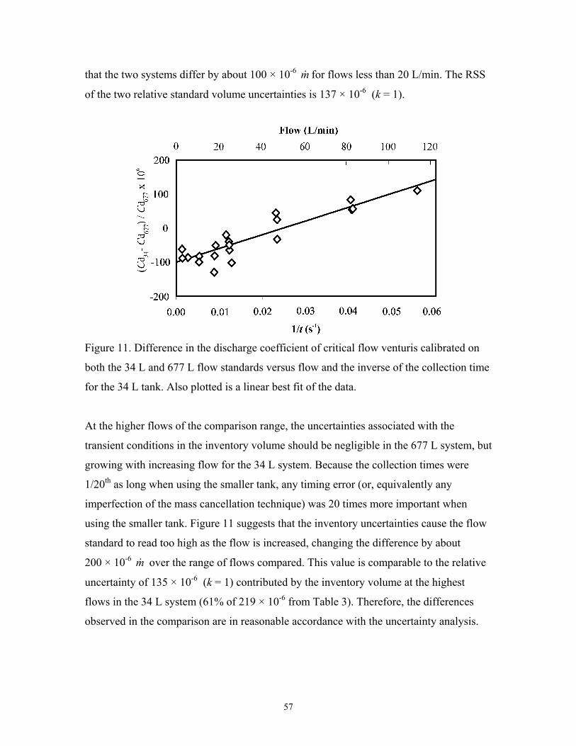
that the two systems differ by about 100 × 10-6 for flows less than 20 L/min. The RSS

of the two relative standard volume uncertainties is 137 × 10

m&-6 (k = 1).

Figure 11. Difference in the discharge coefficient of critical flow venturis calibrated on

both the 34 L and 677 L flow standards versus flow and the inverse of the collection time

for the 34 L tank. Also plotted is a linear best fit of the data.

At the higher flows of the comparison range, the uncertainties associated with the

transient conditions in the inventory volume should be negligible in the 677 L system, but

growing with increasing flow for the 34 L system. Because the collection times were

1/20th as long when using the smaller tank, any timing error (or, equivalently any

imperfection of the mass cancellation technique) was 20 times more important when

using the smaller tank. Figure 11 suggests that the inventory uncertainties cause the flow

standard to read too high as the flow is increased, changing the difference by about

200 × 10-6 over the range of flows compared. This value is comparable to the relative

uncertainty of 135 × 10

m&-6 (k = 1) contributed by the inventory volume at the highest

flows in the 34 L system (61% of 219 × 10-6 from Table 3). Therefore, the differences

observed in the comparison are in reasonable accordance with the uncertainty analysis.

57

Figure 11 also shows the tank comparison results from the perspective of time

measurement uncertainty rather than the mass. We interpreted the comparison results

using the simplified model , where m is the mass collected and t is the collection

time using the 34 L tank. Making the assumption that there exists a constant error in the

mass measurement, δm, for all flows (say due to a tank volume error) and a constant error

in time measurement, δt, for all flows (say due to the time constant of the inventory

pressure sensor), we can derive a simple linear model for the error in mass flow

measurement, i.e.,

tmm /=&

tt

mm

mm δδδ

−=&

&. (17)

Since the mass collected and the mass error are both essentially constant, this model

suggests that a linear function of the inverse of the collection time should fit the tank

comparison data. Such a linear function fits reasonably well, as shown in Fig. 11, and its

slope implies a constant timing error of 4 ms. A timing error of this order is not surprising

because the timing is based on a pressure sensor with a time constant of approximately

20 ms. The standard deviation of a measurement from the best fit line is 24 × 10-6 . m&

The comparison results could be the basis for corrections to the 34 L system. The

intercept of Fig. 11 could be used to change the volume of the 34 L tank and improve the

agreement between the two systems at low flows. The slope could be used to improve

agreement at higher flows. This approach offers the possibility of reducing the

comparison differences to zero with a standard deviation of 24 × 10-6 . However, these

corrections have not been made at the present time for several reasons. The comparison

results are consistent with the uncertainty analysis. Also, despite the success of Eq. 17,

we feel that the inventory uncertainties are more related to pressure and temperature than

time, so it is more appropriate to make improvements in those measurements to reduce

the slope in the comparison data. The volume (or offset) differences can be improved by

repeating and refining the volume expansion process used to determine the 34 L tank

m&

58

size. This approach adheres to the definition of primary standard for both systems since

neither one has been calibrated by a flow measurement against some other flow standard.

During some of the comparison flows, we noticed that the pressure downstream of the

critical flow venturi was significantly higher in the 34 L system than in the 677 L system

(108 kPa vs. 100 kPa) due to the smaller tube size and resultant higher pressure drop. For

some of our venturis (with relatively short diffusers) this pressure difference caused slight

changes in the upstream pressure (and the discharge coefficient), even at conditions well

above the critical pressure ratio. Therefore, our assumption that for the same throat

Reynolds number, the discharge coefficient of the venturi is independent of the

downstream pressure may not be perfectly valid. We suspect that some of the differences

observed between the tanks in Fig. 11 are due to the venturis (even though long diffusers

were used).

In one series of experiments, the trigger pressure difference was purposely varied over a

range from –2 kPa to 27 kPa at a constant flow of 82 L/min in the 34 L system. The

purpose of the test was to measure the dependence of the venturi discharge coefficient on

the trigger pressure difference and hence assess its influence on the inventory volume

uncertainties. The tests showed a relative change of 10 × 10-6 in discharge coefficient for

each 1 kPa change in the trigger pressure difference. Since the largest trigger pressure

difference is less than 3 kPa in the present system, this effect is expected to contribute

only 30 × 10-6 to the flow uncertainty. Therefore the major contributor to the

inventory uncertainty appears to be spatial inconsistency of the pressure and temperature

fields between the start and stop diversions or some other, unknown flow dependent

uncertainty source.

m&

7.2 Multiple Diversions in the 677 L Flow Standard

To confirm that the uncertainty analysis for the inventory volume of the 677 L collection

system was reasonable, we performed CFV calibrations at identical flows following two

different protocols. In the first protocol, the inventory volume was dead-ended at the

59

beginning and end of the collection interval in the usual manner. In the second protocol,

the collection interval was divided into two subintervals, i.e. each flow measurement had

two start and stop diversions. The intermediate dead-end times were set up so that the

pressure transients in the inventory volume still permitted the mass cancellation

procedure. Breaking the collection into two subintervals has the effect of doubling the

uncertainty contribution from the inventory volume. The CFV discharge coefficients

from the two protocols were compared to assess the magnitude of the uncertainties

introduced by the inventory volume and the flow diversion process. Three flows between

300 L/min and 1600 L/min were tested and the differences in discharge coefficient were

all less than 75 × 10-6 as shown in Table 23. m&

Table 23. Differences in CFV discharge coefficients (Cd) for two and one diversion in the

677 L flow standard. Flow (L/min) [Cd (2 diversions) – Cd]/Cd × 106

300 53 ± 25

700 -27 ± 31

1600 75 ± 122

8 Summary

We have given a description of the gas flowmeter calibration services that use the 34 L

and 677 L PVTt primary standards within the NIST Fluid Flow Group. These PVTt

standards were designed to calibrate flowmeters between 1 L/min to 2000 L/min, with

uncertainties between 0.02 % and 0.05 %. See Table 1 for more details about the test

capabilities of the calibration service such as available gases and pressure at the test

section. The 34 L PVTt standard has been used at flows as low as 0.025 L/min.

The intended audience for this document is potential flowmeter calibration customers,

hence we have attempted to address their likely questions. We have described the method

of operation of the primary standard and have given the uncertainty analysis for a mass

flow measurement (see Tables 2 and 3). We have given a description of the standard gas

60

flow calibration, including a sample calibration report, as well as sources for instructions

for submitting a flowmeter for calibration.

The 34 L and 677 L PVTt flow standards have several novel features. The collection

tanks are immersed in a water bath that matches the nominal room temperature and is

stable and uniform to 1 mK. The collection tanks are divided into sections of small

enough diameter that the gas inside them achieves thermal equilibrium with the

surrounding water bath in 20 minutes or less. This reduces the contribution of

temperature to the flow measurement uncertainty to a low level.

Uncertainties related to the inventory volume and the diversion of gas into the collection

tank at the start and stop of a flow measurement have been studied in great detail. A

thermodynamic model of the inventory volume during diversion has been utilized to

understand the large pressure and temperature transients and the importance of sensor

time constants on the flow measurement uncertainty. The flow standard is operated to

achieve “mass cancellation” in the inventory volume, thereby taking advantage of

correlated sensor uncertainties to minimize uncertainty contributions from the inventory

volume. The uncertainty contributions of the inventory volume have been considered

from both the time and mass perspectives.

The volumes of the collection tanks were measured by two methods, a gas gravimetric

method and a volume expansion method. Six gravimetric determinations of the 677 L

collection tank volume made with nitrogen and argon agree with a standard deviation of

16 × 10-6 VT.

A detailed uncertainty analysis for the gas flow standard has been presented The analysis

started with the basis equation utilized to calculate flow in a PVTt system and followed

the propagation of uncertainties method suggested by international standards. The

uncertainties of the sub-components have been examined at a fundamental level.

61

The uncertainty analysis shows that the 677 L system measures mass flow with an

uncertainty between 200 × 10-6 and 300 × 10m& -6 for a pure gas like nitrogen or

argon. The higher uncertainty applies to higher flows as the inventory transients and the

related uncertainties grow larger. For the 34 L tank and pure gases, the uncertainties

range from 440 × 10

m&

-6 to 270 × 10m& -6 m . The uncertainties are larger for the 34 L tank

because the tank volume uncertainty is relatively greater and the inventory volume is

relatively larger for the small system. For pure gas measurements, the largest sources of

uncertainty can be traced to pressure measurement (about 70 × 10

&

-6 P) which is the major

contributor to gas density and tank volume uncertainties. For air flow measurements

using gas from the existing compressor and drier, mass flow uncertainties are about 500 ×

10-6 for both standards and the major contribution is the uncertainty in the moisture

content of the air.

m&

Comparisons between the 34 L and 677 L standards from 3 L/min to 100 L/min show

agreement within 150 × 10-6 m or better. Experiments using single diversions (normal

operation) and double diversions to the collection tank were used to validate the

uncertainty estimates of the 677 L inventory volume and the differences between these

two methods were less than 75 × 10

&

-6 m . The evaluation results along with comparisons

to previously existing gas flow standards support the uncertainty statements for the new

standards.

&

9 References

Carslaw, H. S. and Jaeger, J. C., Conduction of Heat in Solids, 2nd Edition, Clarendon Press, Oxford, pp 198-201, 1946. Coleman, H. W. and W. G. Steele, Experimentation and Uncertainty Analysis for Engineers, John Wiley and Sons, 2nd edition, 1999.

Dymond, J. H. and Smith, E. B., The Virial Coefficients of Pure Gases and Mixtures: A Critical Compilation, Clarendon Press, Oxford, 1980. Harris, R. E. and Johnson, J. E., Primary Calibration of Gas Flows with a Weight / Time Method, Proceedings 2nd International Symposium on Fluid Flow Measurement, Calgary, Canada, pp. 347–358, June, 1990.

62

Hilsenrath, J., Beckett, C. W., Benedict, W. S., Fano, L., Hoge, H. J., Masi, J. F., Nuttall, R. L., Touloukian, Y. S., and Woolley, H. W., Tables of Thermal Properties of Gases, NBS Circular 564, 1955. International Organization for Standardization, International Vocabulary of Basic and General Terms in Metrology, 2nd edition, 1993. International Organization for Standardization, Guide to the Expression of Uncertainty in Measurement, Switzerland, 1996. Ishibashi, M., Takamoto, M., and Watanabe, N., New System for the Pressurized Gas Flow Standard in Japan, Proceedings of International Symposium on Fluid Flow Measurements, AGA, 1985. Jaeger, J. B. and Davis, R. S., A Primer for Mass Metrology, NBS Special Publication 700-1, National Bureau of Standards, Gaithersburg, Maryland, Eq. 20a, pp. 22, 1984. Johnson, A. N., Wright, J. D., Moldover, M. R., and Espina, P. I., Temperature Characterization in the Collection Tank of the NIST 26 m3 PVTt Gas Flow Standard, Metrologia, 40, 211–216, 2003. Kegel, T., Uncertainty Analysis of a Volumetric Primary Standard for Compressible Flow Measurement, 3rd International Symposium of Fluid Flow Measurement, San Antonio, TX, USA, 1995. Lemmon, E. W., Jacobsen, R. T., Penoncello, S. G., and Friend, D. G., Thermodynamic Properties of Air and Mixtures of Nitrogen, Argon, and Oxygen from 60 to 2000 K at Pressures to 2000 MPa, J. Phys. Chem. Ref. Data, 29, (3), 331-362, 2000. Lemmon, E. W., McLinden, M. O., and Huber, M. L., Refprop 23: Reference Fluid Thermodynamic and Transport Properties, NIST Standard Reference Database 23, Version 7, National Institute of Standards and Technology, Boulder, Colorado, 2002. Marshall, J. L., NIST Calibration Services Users Guide 1998, NIST Special Publication 250, January, 1998. Moldover, M. R., Trusler, J. P. M., Edwards, T. J., Mehl, J. B., and Davis, R. S., Measurement of the Universal Gas Constant R Using a Spherical Acoustic Resonator, NIST J. of Res., 93, (2), 85–143, 1988. Olsen, L. and Baumgarten, G., Gas Flow Measurement by Collection Time and Density in a Constant Volume, Flow: Its Measurement and Control in Science and Industry, Instrument Society of America, Pittsburgh, PA, USA, pp. 1287–1295, 1971.

63

Patterson, J. B. and Morris, E. C., Measurement of Absolute Water Density, 1° C to 40° C, Metrologia, 31, pp. 277-288, 1994. Trusler, J. P. M., Wakeham, W. A., and Zarari, M. P., Model Intermolecular Potentials and Virial Coefficients Determined from the Speed of Sound, Molecular Physics, 90, (5), pp. 695–703,1997. Wright, J. D., The Long Term Calibration Stability of Critical Flow Nozzles and Laminar Flowmeters, National Conference of Standards Laboratories Conference Proceedings, Albuquerque, NM, USA, pp. 443-462, 1998. Wright, J. D. and Mattingly, G. E., NIST Calibration Services for Gas Flow Meters: Piston Prover and Bell Prover Gas Flow Facilities, NIST Special Publication 250-49, National Institute of Standards and Technology, Gaithersburg, Maryland, August, 1998. Wright, J. D., Gas Flow Measurements and Standards: Development and Validation of a PVTt Primary Gas Flow Standard, Doctoral thesis to Kogakuin University, Tokyo, Japan, September, 2003A. Wright, J. D., What Is the “Best” Transfer Standard for Gas Flow?”, FLOMEKO, Groningen, the Netherlands, May, 2003B.

64

NIST Test Number: 836-123456-03-01 Page 1 of 6 Calibration Date: July 2, 2003

Appendix: Sample Calibration Report

REPORT OF CALIBRATION

FOR

A CRITICAL FLOW NOZZLE

July 7, 2003

Mfg.: Meter Builders, Inc. Serial No: 1234

Throat Diameter: 0.125 in (0.3175 cm)

submitted by

Flowmasters, Inc. Metertown, MD

Purchase Order No. A123 dated June 23, 2003

The flow meter identified above was calibrated by flowing filtered dry air at a constant rate through the flow meter and then into a volumetric prover (the NIST 677 L PVTt standard). The PVTt standard determines mass flow, , by measuring the change in density of gas diverted into a known volume for a measured period of time.

m&1 The flow

meter was tested at five flows and at each flow, three (or more) measurements were gathered on two different occasions and used to produce averages at each of these flows. As a result, the tabulated data for this test are averages of six or more individual calibration measurements. The nozzle was installed in an assembly that meets the ISO Standard for critical nozzles2 and a photograph of the installation is shown in Figure 1. The nozzle temperature ( and pressure were measured with NIST sensors, (Keithley SN 687848, thermistor #3, and Paroscientific SN 75971). Stagnation temperature, T was calculated from the measured temperature via the following equation, using a recovery factor,

)1T)( 1P

0

r , of 0.75:

( )T T M r0 121 1

21= ⋅ +

−⋅ ⋅ −

γ (1)

1 Wright, J. D., Johnson, A. N., and Moldover, M. R., Design and Uncertainty Analysis for a

PVTt Gas Flow Standard, J. Res. Natl. Inst. Stand. Technol., 108, 21-47, 2003. 2 Measurement of Gas Flow by Means of Critical Flow Venturi Nozzles, ISO 9300: 1990 (E),

International Organization for Standardization, Geneva, Switzerland, 1990.

REPORT OF CALIBRATION Gas Flow Meters Flowmasters, Inc. Purchase Order No. A123

and the stagnation pressure, , was calculated via the equation: 0P

P P M0 12 1

1 12

= ⋅ +−

⋅

−γγγ

(2)

where γ is the specific heat ratio and M is the Mach number in the approach pipe, both based on and T . The largest of these corrections is 0.0067% for pressure. 1P 1

Figure 1. A photograph of the flow meter installation.

The Reynolds number is included in the tabulated data and it was calculated using the following expression:

µπ ⋅⋅⋅

=d

mRe&4 (3)

where is the mass flow of gas, is the nominal nozzle throat diameter, and &m d µ is the gas viscosity, all in consistent units so that is dimensionless. The viscosity of the gas was calculated using best-fit equations which are based on the NIST gas properties database

Re

3: 3

032

02010 TaTaTaa +++=µ (4)

3 Lemmon, E. W., McLinden, M. O., and Huber, M. L., Refprop 23: Reference Fluid

Thermodynamic and Transport Properties, NIST Standard Reference Database 23, Version 7, National Institute of Standards and Technology, Boulder, Colorado, 2002.

NIST Test Number: 836-123456-03-01 Page 2 of 6 Calibration Date: July 2, 2003

REPORT OF CALIBRATION Gas Flow Meters Flowmasters, Inc. Purchase Order No. A123

where µ has units g / (cm s), and T is in K. The polynomial coefficients, a are in turn polynomial functions of pressure

0 i

303

202010 PbPbPbba iiii

i +++= (5)

where is in kPa and the coefficients for dry air are: 0P ib j

-1.48711900E-06 2.36550580E-08 -4.74728350E-11 3.80951780E-14 8.03433280E-07 -2.06447690E-10 4.86819380E-13 -3.87442880E-16

-7.32108840E-10 6.60598760E-13 -1.65670740E-15 1.31012510E-18

( ) =µib j

4.44444440E-13 -7.23905720E-16 1.87289560E-18 -1.47306400E-21 (6)

where i number and number. row= column=j The discharge coefficient C was calculated from the expression: d

Cm R Td P Cd =⋅ ⋅ ⋅⋅ ⋅ ⋅ ∗

4 02

0

&

π (7)

where R is the gas constant (the universal gas constant, 8.314471 J / (mol K), divided by the gas molecular weight, 28.9646431 g/mol). The critical flow factor, C∗ , was calculated from the expression:

11

*

12 −

+

+=

γγ

γγC (8)

where γ is the specific heat ratio, calculated using the same system of polynomials described above with the following coefficients:

1.40035540E+00 2.31594790E-04 2.32361020E-08 3.48369500E-13 -2.51273630E-06 -1.63018610E-06 -2.01773710E-10 -4.02631530E-15

9.40776360E-08 4.19213690E-09 5.90056690E-13 1.42526470E-17

( ) =γib j

-3.01845240E-10 -3.79086500E-12 -5.81559640E-16 -1.61335590E-20

(9)

The calibration results are presented in the following table and figure.

NIST Test Number: 836-123456-03-01 Page 3 of 6 Calibration Date: July 2, 2003

REPORT OF CALIBRATION Gas Flow Meters Flowmasters, Inc. Purchase Order No. A123

0.9780

0.9800

0.9820

0.9840

0.9860

0.9880

0.9900

35,000 85,000 135,000 185,000 235,000 285,000

Re

Cd

Figure 2. Calibration results for 0.125 in (0.3175 cm), SN 1234 nozzle Table 1. Calibration results for 0.125 in (0.3175 cm), SN 1234 nozzle from the 677 L

PVTt standard.

0P [kPa]

0T

[K] m&

[lbm/s] ∗C

[] Re []

dC []

rU [%]

104.07 295.73 0.004189 0.68505 41471.1 0.9808 0.08

249.69 295.26 0.010117 0.68550 100147.9 0.9859 0.08

399.90 294.87 0.016256 0.68597 160854.2 0.9877 0.08

546.52 294.63 0.022261 0.68643 220116.4 0.9887 0.08

685.88 294.49 0.027979 0.68686 276392.8 0.9893 0.08 An analysis was performed to assess the uncertainty of the results obtained for the meter under test.4, 5, 6 The process involves identifying the equations used in calculating the 4 International Organization for Standardization, Guide to the Expression of Uncertainty in

Measurement, Switzerland, 1996 edition. 5 Taylor, B. N. and Kuyatt, C. E., Guidelines for Evaluating and Expressing the Uncertainty of

NIST Measurement Results, NIST TN 1297, 1994 edition.

NIST Test Number: 836-123456-03-01 Page 4 of 6 Calibration Date: July 2, 2003

REPORT OF CALIBRATION Gas Flow Meters Flowmasters, Inc. Purchase Order No. A123

calibration result (measurand) so that the sensitivity of the result to uncertainties in the input quantities can be evaluated. The 67 confidence level uncertainty of each of the input quantities is determined, weighted by its sensitivity, and combined with the other uncertainty components by root-sum-square to arrive at a combined uncertainty (U ). The combined uncertainty is multiplied by a coverage factor of 2.0 to arrive at an expanded uncertainty (U ) of the measurand with approximately 95 confidence level.

%

c

e % As described in the references, if one considers a generic basis equation for the measurement process, which has an output, , based on input quantities, , y N ix

),,,( 21 Nxxxyy K= (10)

and all uncertainty components are uncorrelated, the normalized expanded uncertainty is given by,

( ) ( ) ( )∑=

==

N

i i

ii

ce

xxusk

yyUk

yyU

1

22 (11)

In the normalized expanded uncertainty equation, the u are the standard uncertainties of each input, and are their associated sensitivity coefficients, given by,

s)'x( i

s'si

yx

xys i

ii ∂

∂= (12)

The normalized expanded uncertainty equation is convenient since it permits the usage of relative uncertainties (in fractional or percentage forms) and of dimensionless sensitivity coefficients. The dimensionless sensitivity coefficients can often be obtained by inspection since for a linear function they have a magnitude of unity. For this calibration, the uncertainty of the discharge coefficient has components due to the measurement of the mass flow by the primary standard, ( ) %025.0=mu & ,7 as well as the pressure, u , and temperature, ( ) %02.0=P ( ) %03.0=Tu , measurements at the meters under test. The sensitivity coefficients for mass flow and pressure are 1, and the sensitivity coefficient for temperature is ½. This uncertainty analysis assumes that the user will use the same values for the throat diameter and the critical flow factor given herein and that the uncertainties in these quantities are correlated and cancel. To measure the reproducibility8 of the test, the standard deviation of the discharge 6 Coleman, H. W. and Steele, W. G., Experimentation and Uncertainty Analysis for Engineers,

John Wiley and Sons, 2nd ed., 1999. 7 Wright, J. D., Johnson, A. N., and Moldover, M. R., Design and Uncertainty Analysis for a

PVTt Gas Flow Standard, J. Res. Natl. Inst. Stand. Technol., 108, 21-47, 2003. 8 Reproducibility is herein defined as the closeness of agreement between measurements with the

flow changed and then returned to the same nominal value.

NIST Test Number: 836-123456-03-01 Page 5 of 6 Calibration Date: July 2, 2003

REPORT OF CALIBRATION Gas Flow Meters Flowmasters, Inc. Purchase Order No. A123

NIST Test Number: 836-123456-03-01 Page 6 of 6 Calibration Date: July 2, 2003

coefficient at each of the nominal flows was used to calculate the relative standard uncertainty (the standard deviation divided by the mean and expressed as a percentage). The reproducibility was root-sum-squared along with the other uncertainty components to calculate the combined uncertainty. Using the values given above results in the expanded uncertainties listed in the data table and shown as error bars in the figure. For the Director, National Institute of Standards and Technology Dr. Pedro I. Espina Leader, Fluid Flow Group Process Measurements Division Chemical Science and Technology Laboratories