Embed Size (px)
Citation preview

MULTIPLE IMPELLER GAS-LIQUID CONTACTORS48
4Gas Dispersion Phenomena and
Bubble Motion in Agitated VesselsThe performance of gas dispersion determines the bubble size and exerts a great
influence to the mass transfer rate within the gas-liquid contactor, which severely affects the
reaction rate and product yield as a result. However, the mechanism of gas dispersion by
impeller in a mechanically agitated vessel was quite ambiguous until the hydrodynamics of
liquid flow behind the blade has been examined in late sixties. In this chapter, the gas
dispersion phenomena of different impellers and the bubble motion within the single and
multiple impeller systems are discussed in detail to offer a guideline for the impeller
selection.
4.1 States of gas dispersion and their transitions within stirred vessel
From the visual observation, Nienow et al. (1977, 1985) delineated the five states of gas
dispersion within the single Rushton gas-liquid stirred vessel as shown in Fig. 4.1-1 and
categolized them as: (a) no gas dispersion is achieved, large bubbles escape along along the
impeller axis; (b) sufficient dispersion for the upper part of the vessel to act as a bubble
column; (c) gas circulation can be seen in the upper part of the vessel with some movement
into the lower region; (d) circulation of bubbles occurs throughout the vessel; (e) at a still
higher impeller rotational speed, secondary circulation loop of bubbles appears at the location
close to the surface.
In the operation of gassed mechanically stirred tanks, it has long been found that the
flooding phenomenon occurs when the power input by agitation is too low to disperse a
certain gassing flow rate. Below the flooding point, gas dispersion becomes inefficient, so that
both the gas holdup and the gas-liquid mass transfer rate decrease sharply, which is an
undesirable condition and need to be avoided in gas-liquid mixing operations. Designers
usually need a specific set of data of the minimum impeller speed at which flooding
phenomenon is overcome.

Gas Dispersion Phenomena and Bubble Motion in Agitated Vessels 49
Fig. 4.1-1 The five characteristic stages of gas dispersion.(Nienow et al. 1977).
Various methods for estimating the flooding condition are summarized in Table 4.1-1. It
was after 1970, that more attention was paid to this subject when the mechanism of the
sparged gas dispersion was of primarily interest. It is interesting to compare the changes in the
definitions and the correlation equations before and after 1970. Before 1970, a minimum
impeller rotational speed was observed below which the impeller exerts no influence on the
transport properties such as the overall gas holdup, the specific gas-liquid interfacial area, and
the overall volumetric mass transfer coeffcient. The correlations for the minimum speed
presented in this period contain the effect of the physical properties (surface tension, density),
but not the gas sparged rate. On the contrary, the gas sparged rate has been one of the most
important factors to the correlations presented lately and the physical properties play no role
in the recent correlations. The most common method used recently to determine the flooding
condition is the impeller power consumption curve method developed by Nienow et al.
(1977).
Fig. 4.1-2 The plot of Pg/Po vs.. aeration number (Calderbank, 1958).

MULTIPLE IMPELLER GAS-LIQUID CONTACTORS50
Table 4.1-1 Summary of impeller flooding condition for Rushton turbine impeller.
Author )(cmTTD Metho
dResults
Westerterpet Al. (1963)
14-90 0.2-0.7 SPAR( )( )4
1ρσgDTbaDNM += a=1.22 b=1.25, for turbine
a=2.25 b=0.68, for paddleDierendonck et al.
(1968)15.6-92.3 1/3 HOUP 25.1219.0 −= DTNM for pure liquid and T<1.0 m
( ) ( ) 241
21
2 −= DghTNM ρσ for pure liquid and T>1.0 m
( )41
2 ρσgTDN M−= for ionic solution
Smith et al. (1977) 44-183 1/3-1/2 CAVY21
99.0 DN F =Nienow et al.
(1977)29 1/3-2/3 PWRO
241
21
4 −= DTQN FGreaves and
Kobbacy (1981)20.3 0.375-2/3 SMEM 72.12.029.0 −= DTaQN F a=1.52, for pure liquid
a=1.66, for ionic solutionWiedmann et al.
(1980, 1981, 1982)45 1/3 PWAR 207.1283.0694.2 −= DQN F
Ismail et al. (1984) 40 1/3 PWRO 146.1
22
22
051.0⎪⎭
⎪⎬⎫
⎪⎩
⎪⎨⎧
⎟⎟⎠
⎞⎜⎜⎝
⎛−⎟
⎟⎠
⎞⎜⎜⎝
⎛=
inA
F
DDD
WDN
gDN
b
Nienow et al.(1985)
29-120 0.22-0.58 PWAR ( ) ( ) 35.331
40322. DTDQgN F =Lu and Chen
(1985)28.8 1/3 VELO 8.13.054.0 −= DQN F
Warmoeskerkenand Smith (1985)
44-120 0.4 MPRO ( ) 314941.0 DQgN F =Wong et al. (1986) 29 1/3 PWAR 8.13.075.0 −= DQN F
CAVY: large cavity unstable condition.HOUP: overall gas holdup.PWAR: power curve under constant impeller speed and varying gas rate.PWRO: power curve under constant gas rate and varying impeller speed.SPAR: specific gas-liquid interfacial area.SMEM: semi-empirical technique.VELO: volume averaged turbulent fluctuating velocity.MPRO: mini propeller.
It is not clear who was the first person introduced the word "FLOODING" to aerated
stirred tank operations, but we know that Calderbank (1958) first mentioned the word
"FLOODING" in his paper as shown in Fig.4.1-2.
Westerterp et al. (1963) measured the gas absorption rates as shown in Fig.4.1-3, using
reactions between a sulfite solution and absorbed oxygen and between a sodium hydroxide
solution and absorbed carbon dioxide in a gas-liquid contactor agitated with the turbine, the
paddle, and the propeller impellers of various ratio of tanks to impeller diameter. They found
that the influence of the impeller rotational speed on the specific absorption rate could be
divided into two regions. (a) A region without agitation effect-at very low impeller speeds the
specific absorption rate does not improve due to the stirring until a certain minimum speed is

Gas Dispersion Phenomena and Bubble Motion in Agitated Vessels 51
surpassed. In this region the specific absorption rate depends on the gas load and the type of
sparger, but not on the impeller speed. (b) A region with agitation effect-as the impeller speed
surpasses the minimum speed, the specific absorption rate increases quickly and linearly with
increase in the impeller speed. They pointed out that at very low impeller speeds the gas is not
dispersed at all. In the neighborhood of the minimum impeller speed some effect was seen;
the amount of gas bubbles below the stirrer is still very low, and fine bubbles are only found
in the region above the impeller. Once the minimum speed has been surpassed, the dispersion
gets better and more homogeneous. In accordance with this result, they proposed the idea of
the “minimum impeller speed”. The minimum impeller speed was obtained by linear
extrapolating the specific absorption rate towards zero and finding the corresponding impeller
speed. From the result of the influence of the impeller diameter on the specific absorption rate,
it was found that at increasing impeller diameters the value of the minimum impeller speed
becomes lower. The “minimum agitation rate” was then defined as the product of the
minimum impeller speed and the impeller diameter. They presented the first correlation for
the minimum agitation rate as :
NoD = (A+BT/D)(gσ/ρ)0.25 (4.1-1)
where A=1.22 and B=1.25 for turbine impeller; A=2.25 and B=0.68 for paddle impeller.
Fig. 4.1-3 The effect of impeller speed on oxygen absorption into sulfite solution(Westerterp et al., 1963).
One of the shortcomings of the above correlation is that it does not take the influence of
the gas sparging rate on the minimum agitation rate into account. Van Dierendonck et al.
(1968) determined the minimum impeller speed from the measurement of the overall gas
holdup as shown in Fig. 4.1-4. They pointed out that the gas bubbles from a gas distributor

MULTIPLE IMPELLER GAS-LIQUID CONTACTORS52
were dispersed and the overall gas holdup started to increase with impeller speed as the
impeller speed passed a certain value. They obtained the minimum impeller speed by linearly
extrapolating the overall gas holdup towards zero and proposed the following correlations.
(1) For pure liquid
NoD2 =0.07gT1.5 for T<1.0 (4.1-2)
NoD2 =2.0(H’T)0.5(gσ/ρ)0.25 for T>1.0 (4.1-3)
where H’ is the liquid height above the impeller.
(2) For electrolyte solutions
NoD = (aD+bT)(gσ/ρ)0.25 (4.1-4)
where a is very small figure and b is nearly equal to unity.
Fig. 4.1-4 The plot of N vs. gas holdup (Van Dierendonck et al., 1968).
Their correlations did not take into account the influence of the sparging rate on the
minimum impeller speed either. A strict definition of "IMPELLER FLOODING" first
appeared in Rushton and Bimbinets’ work in 1965. Their definition is one of the most
well-known ones and has been referred to very often by later investigators. They found that at
a given total power input, gas holdup increases with air flow rate up to a critical value beyond
which gas holdup decreases sharply and the sparged gas is not well distributed. At a constant
air rate, if (Pg/V) is decreased, larger and larger bubbles will be formed; the impeller is less
and less able to disperse the air throughout the tank properly. When (Pg/V) has decreased to a
critical value, the flow pattern changes suddenly; it is no longer a horizontal flow of gas
bubbles starting from the impeller and reaching the walls.There are no bubbles present in the
large space below and around the impeller. Very large bubbles rise to the surface along the
impeller axis. They stated this state as "FLOODED". They also pointed out the hysterisis
phenomenon of flooding. When the impeller speed is decreased from a high point, flooding
Gas Dispersion Phenomena and Bubble Motion in Agitated Vessels 53
occurs at a lower (Pg/V) value below which dispersion is not likely; tthen the impeller speed is
increased from a low point, flooding occurs at a higher (Pg/V) value beyond which flooding is
also unlikely; Both critical (Pg/V) values were found to be proportional to (D/T) for (D/T)
between 0.26 and 0.44. The ratio of these two critical values was found to be 1.33. These two
critical (Pg/V) values increase with increasing air rate. It is really a pity that no correlation was
given in their paper.
The mechanisms of gas dispersion and the developments of various kinds of gas cavities
has been intensively studied by Bruijn et al.(1974) They found that large cavities can exist
only when the Froude number exceeds 0.1; otherwise, large bubbles will escape from the
cavities as a result of buoyancy forces. This result has been used by Vant Riet and
NF= (0.1g / D)0.5 (4.1-5)
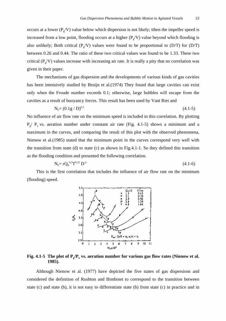
No influence of air flow rate on the minimum speed is included in this correlation. By plotting
Pg/ Po vs. aeration number under constant air rate (Fig. 4.1-5) shows a minimum and a
maximum in the curves, and comparing the result of this plot with the observed phenomena,
Nienow et al.(1985) stated that the minimum point in the curves correspond very well with
the transition from state (d) to state (c) as shown in Fig.4.1-1. So they defined this transition
as the flooding condition and presented the following correlation.
NF= rQS0.5T0.25 D-2 (4.1-6)
This is the first correlation that includes the influence of air flow rate on the miminum
(flooding) speed.
Fig. 4.1-5 The plot of Pg/Po vs. aeration number for various gas flow rates (Nienow et al.1985).
Although Nienow et al. (1977) have depicted the five states of gas dispersions and
considered the definition of Rushton and Bimbinet to correspond to the transition between
state (c) and state (b), it is not easy to differentiate state (b) from state (c) in practice and in
MULTIPLE IMPELLER GAS-LIQUID CONTACTORS54
many cases the differentiation between these two states is not possible. However, the
transition from state (a) to state (b) is always very obvious. In this respect, the definition of
impeller flooding given by Rushton and Bimbient may be considered to be equivalent to the
transition from state (b) to state (a), though Nienow et al. considered that to correspond to the
transition from state (c) to state (b).
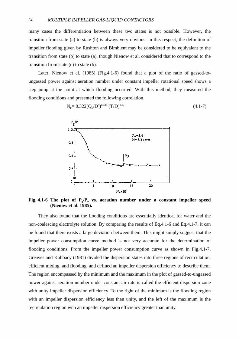
Later, Nienow et al. (1985) (Fig.4.1-6) found that a plot of the ratio of gassed-to-
ungassed power against aeration number under constant impeller rotational speed shows a
step jump at the point at which flooding occurred. With this method, they measured the
flooding conditions and presented the following correlation.
NF= 0.322(QS/D4)0.333 (T/D)1.67 (4.1-7)
Fig. 4.1-6 The plot of Pg/Po vs. aeration number under a constant impeller speed(Nienow et al. 1985).
They also found that the flooding conditions are essentially identical for water and the
non-coalescing electrolyte solution. By comparing the results of Eq.4.1-6 and Eq.4.1-7, it can
be found that there exists a large deviation between them. This might simply suggest that the
impeller power consumption curve method is not very accurate for the determination of
flooding conditions. From the impeller power consumption curve as shown in Fig.4.1-7,
Greaves and Kobbacy (1981) divided the dispersion states into three regions of recirculation,
efficient mixing, and flooding, and defined an impeller dispersion efficiency to describe them.
The region encompassed by the minimum and the maximum in the plot of gassed-to-ungassed
power against aeration number under constant air rate is called the efficient dispersion zone
with unity impeller dispersion efficiency. To the right of the minimum is the flooding region
with an impeller dispersion efficiency less than unity, and the left of the maximum is the
recirculation region wnh an impeller dispersion efficiency greater than unity.

Gas Dispersion Phenomena and Bubble Motion in Agitated Vessels 55
Fig. 4.1-7 The plot of Pg/Po vs. NA for various gassing rates (Greaves and Kobbacy,1981).
They derived semi-empirically the following correlation for the following condition. For
pure water,
NF= 1.52T0.2QS0.29D-1.72 (4.1-8)
For ionic solutions,
NF= 1.66T0.2QS0.29D-1.72 (4.1-9)
The impeller power consumption curve method was also employed by Ismail et al. (1984)
to determine the flooding condition They plotted the ratio of gassed-to-ungassed power
against the impeller speed, instead of against the aeration number and calculated the flooding
conditions from the maximum of the curves.
Fig. 4.1-8 Variation of average turbulent fluctuating velocity by changing gassing ratesunder a given impeller speed.
MULTIPLE IMPELLER GAS-LIQUID CONTACTORS56
Lu and Chen (1986) were the first ones to attempt to measure the mean and the root-
mean-square (rms) velocities of the liquid in an aerated stirred tank using hot film
anemometry with a conical film probe. At constant rotational speed, the power consumpnon
per unit mass always decreases as the au flow rate increases. The volume average velocity,
<u’>, was found to have a curious relationship with P/V in an aerated agitated system. Figure
4.1-8 shows a dumping behavior occurred at some critical value of Pg/V for various rotational
speeds.
When they gradually reduced the air flow rate at a constant rotational speed, the Pg/V
gadually increased and the <u’> vs. Pg/V proceeded along the lower line. Further decrease in
the air flow rate to some critical value, the value of <u’> abruptly jumped from the lower line
to the upper line, and the transition of a poor dispersion of air in the system to a
well-dispersed status could be observed in this instance. The magnitude of critical Pg/V
increased as N increased. This is denoted by the vertical dash line in this figure. The figure
strongly suggests that at a given Pg/V, there exists a critical revolutional speed N, or an
appropriate aeration number to have good dispersion of air in the system.
They defined this jump as the flooding condition and gave a correlation as follows:
NF= QS0.3D-1.8 (4.1-10)
The use of the rms fluctuating velocity to determine the flooding condition is an effective
tool. It is not difficult to realize how the liquid velocity will change when the impeller is
flooded. All the previous investigations confirmed the fact that the impeller does not disperse
the sparged gas and eases to produce a radial liquid velocity to carry the sparged gas bubbles
to the vessel wall horizontally when flooding occurs. This implies that the impeller pumps
nothing out of it. Under this circumstance, it is reasonable to expect that there will exist a
drastic change in the liquid velocity when the impeller is operated in the vicinity of flooding
condition. On the other hand, the use of the volume averaged value of the liquid velocity may
be inappropriate because impeller flooding condition is, in essence, a feature pertaining to the
impeller itself, though it may influence the overall performance in the tank.
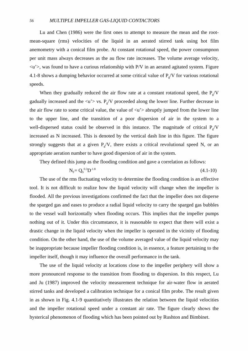
The use of the liquid velocity at locations close to the impeller periphery will show a
more pronounced response to the transition from flooding to dispersion. In this respect, Lu
and Ju (1987) improved the velocity measurement technique for air-water flow in aerated
stirred tanks and developed a calibration technique for a conical film probe. The result given
in as shown in Fig. 4.1-9 quantitatively illustrates the relation between the liquid velocities
and the impeller rotational speed under a constant air rate. The figure clearly shows the
hysterical phenomenon of flooding which has been pointed out by Rushton and Bimbinet.
Gas Dispersion Phenomena and Bubble Motion in Agitated Vessels 57
Fig. 4.1-9 The hysterisis phenomenon of impeller discharge velocity between floodingstage and dispersion stage.
From the intersections of these two curves, two flooding conditions can be obtained; one
is the lowest limit of flooding below which dispersion is unlikely to happen; the other is the
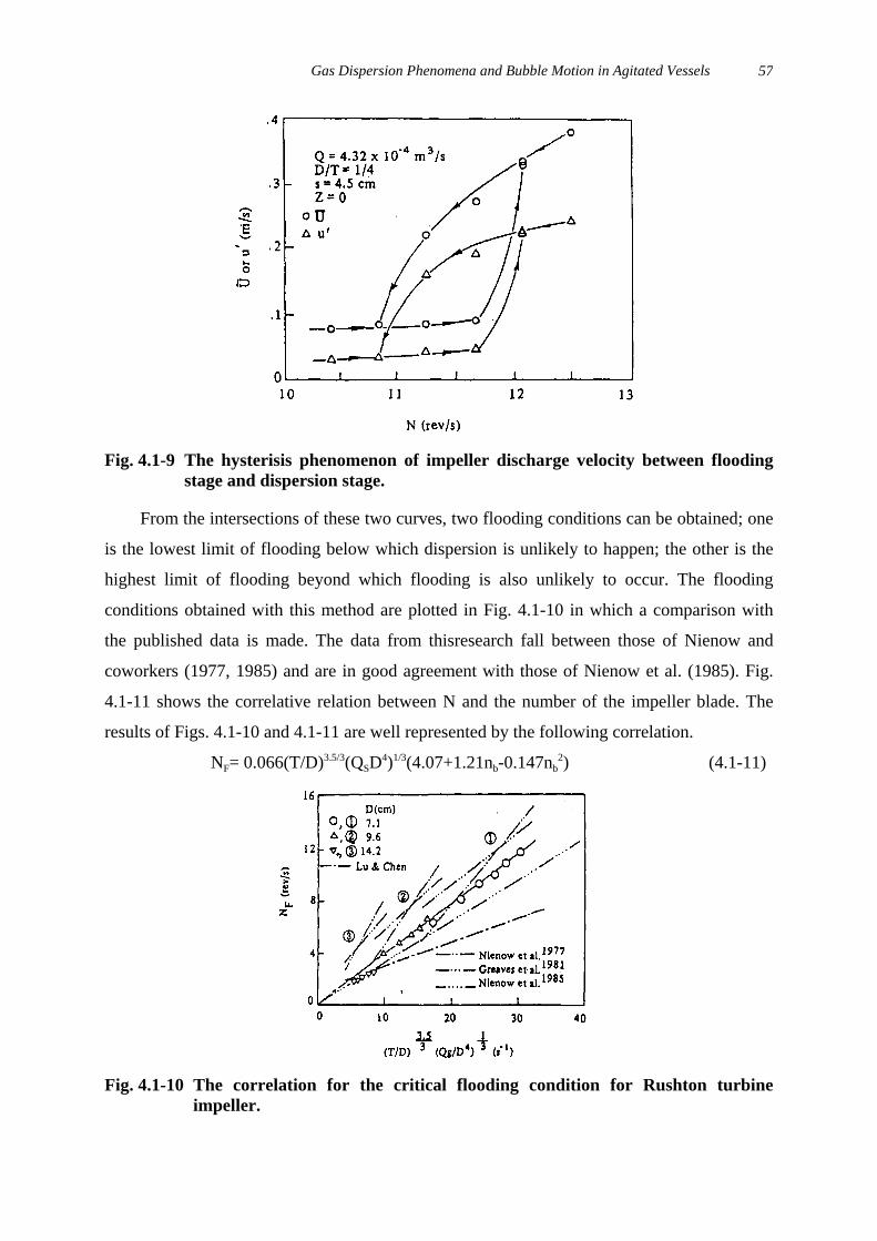
highest limit of flooding beyond which flooding is also unlikely to occur. The flooding
conditions obtained with this method are plotted in Fig. 4.1-10 in which a comparison with
the published data is made. The data from thisresearch fall between those of Nienow and
coworkers (1977, 1985) and are in good agreement with those of Nienow et al. (1985). Fig.
4.1-11 shows the correlative relation between N and the number of the impeller blade. The
results of Figs. 4.1-10 and 4.1-11 are well represented by the following correlation.
NF= 0.066(T/D)3.5/3(QSD4)1/3(4.07+1.21nb-0.147nb2) (4.1-11)
Fig. 4.1-10 The correlation for the critical flooding condition for Rushton turbineimpeller.

MULTIPLE IMPELLER GAS-LIQUID CONTACTORS58
Fig. 4.1-11 The correlation of the critical impeller flooding velocity interns of D, NA andnumber of blades.
Transition conditions determined by bubble size distribution against gas flow number
In examining bubble size distribution in aerated stirred vessels, Lu et al. (1993) found
that the transition rotational speed of impeller can be determined from the plots of Sauter
mean diameter of bubbles vs. Fl (aeration or gas flow number). The typical plots are shown in
Figs.4.1-12, 4.1-13 and 4.1-14, for the upper circulation region of the impeller. At a given QS,
32D first decreases to a minimum value as Fl decreases (that is, increases in N), then
increases to higher value as N continuously increases when the impellers have four and six
blades.
This fact demonstrates that if the value of N is smaller than that corresponding to the
minimum 32D , the negative pressure generated behind the blade is not strong enough to
capture all the sparged gas, and the pumping capacity of the impeller is not high enough to
recirculate of the dispersed bubbles, thus the most dispersed bubbles rise directly to the free
surface. Consequently, the bubble sizes at this stage are dominated by the dispersion ability of
the impeller, and the value of D32 decreases as N increases. As observed, this status of gas
dispersion is within stage (b) and stage (c) as shown in Fig.4.1-1. If the value of N is larger
than the value of N corresponding to the minimum 32D , the pumping capacity of the
impeller will reach a value to at which stronger circulation of both liquid and gas is generated,
whose flow pattern corresponds to stage (d) in Fig 4.1-1. Thus the size of the bubbles will
increase because the circulation of bubbles will enhance their coalescence. From the
description given here, it is seen that the value of the rotational speed corresponding to the
minimum 32D appearing in the plots of 32D vs. Fl is a transition speed at which the status
of gas dispersion of the system shifts from stage (c) to stage (d) and can be defined as NC. Due

Gas Dispersion Phenomena and Bubble Motion in Agitated Vessels 59
to the circulation flow of fluid, the major control factor for the size of bubbles in this region
will be changed from gas dispersion by impeller to the degree of coalescence.
Fig. 4.1-12 32D vs. Fl for nb=4 in the upper circulation region at various gassing rates.
Fig. 4.1-13 32D vs. Fl for nb=6 in the upper circulation region at various gassing rates.
Fig. 4.1-14 32D vs. Fl for nb=8 in the upper circulation region at various gassing rates.

MULTIPLE IMPELLER GAS-LIQUID CONTACTORS60
The values of NC defined here are quite different from the values of Ncd proposed by
Nienow et al. (1977) as shown in Table 4.1-2. The difference is probably caused by the
difference in layout of the impeller and design of the spargers. Under experimental conditions
in this study, the characteristics of gas dispersion of the eight-blade impeller system has
overpassed stage (c); i e. most data are beyond stage (d), and the curves of NC vs., Fl show a
different trend if they are compared with the plots of the four- And six-blade impellers. At a
given QS, 32D in smaller N or a larger value of Fl tends to increase to a maximum value,
then to decrease as N increases. Comparing this result with the relationship between Pg/Po and
Fl, it is noted that the maximum 32D is found near the other transition point, NR a
rectrculation point defined by Nienow et. al. (1977)(i.e. the transition region point from stage
(d) to stage (e) in Fig. 4.1-1), NR lines are also given in Figs 4.1-12 and 4.1-13. Therefore, the
change of 32D in this region at a given QS can be explained as that, even at the lower N, the
eight-blade impeller still pumps enough fluid to provide a circulatory flow, which can provide
32D up to the maximum value. When the increase of N goes beyond the maximum 32D or
the point of NR, part of the recycle bubbles are sucked into the impeller and redispersed by the
impellers which reduce 32D . Therefore, the mechanism of gas dispersion by the trailing
vortex again controls the size of bubbles.
Table 4.1-2 Comparison of transitional speed for gas dispersion stage (c) to stage (d) inFig.4.1-1.
smQg 3510× 3.33 5.05 7.60 10.00 12.50)(rpsNcd 1.383 2.25 2.75 3.17 3.53)(rpsNc 4.70 4.75 5.12 5.18 5.63
( ) ( ) 5.05.020.0: FrT
DFlNcd = defined by Nienow et al. 12)
:cN defined in this study
For the lower circulation region, Since bubbles scarcely appear in this region until the
status of gas dispersion reaches stage (c) shown in Fig. 4.1-1, only smaller bubbles can be
seen at lower N. To examine the role of recirculation in bubble-size distribution in this region,
plots of 32D vs. Fl determined for this region are shown in Fig.4.1-15. For a given QS and
lower N, the increase in N provides a stronger recirculation of fluids which enhances the
coalescence of the bubbles; thus 32D increases to a maximum value. Beyond this maximum
point, 32D will decrease because when N increases, the enhanced circulation flow will
promote redispersion of bubbles by the impeller. These trends coincide with the results of

Gas Dispersion Phenomena and Bubble Motion in Agitated Vessels 61
Zhang et al.(1989). Therefore, the bubble sizes in this region are dominated be the strength of
the circulation of fluid, and NR corresponding to the maximum 32D can be seen as a
transitional speed of the gas dispersion from stage (d) and (e) in Fig. 4.1-1.
Fig. 4.1-15 32D vs. Fl for various impellers in the upper circulation region at variousgassing rates.
4.2 Transitions of ventilated cavities
4.2.1 Cavity structures behind the blade of the Rushton trubine impeller
The rotation of a disc turbine generates a pair of rolling vortices behind each blade
(Takeda and Hoshino,1966 Rennie and Valentin, 1968; Nienow and Wisdom, 1974; Van't
Riet and Smith, 1973, 1975). In low gas flow rates, these vortices suck in the sparged gas to
form gas cavities and then disperse the gas through their dispersive ends as small bubbles.
The cavities play a very important role in gas-phase mixing as well as in gasphase dispersion.
The cavities were classified into three categories: vortex cavity, clinging cavity, large cavity
as shown in Fig.4.2-1 by Bruijn et al. (1974) according to the shape and size of the cavities.
Fig. 4.2-1 Transition of cavities behind the blades (Bruijin et al. ,1974).
MULTIPLE IMPELLER GAS-LIQUID CONTACTORS62
This figure also illustrates how these cavities related to power drawn by the impeller and
gas flow number. They pointed out that the number of large cavities goes from one through
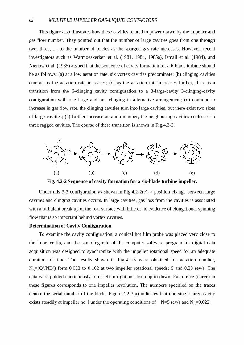
two, three, .... to the number of blades as the sparged gas rate increases. However, recent
investigators such as Warmoeskerken et al. (1981, 1984, 1985a), Ismail et al. (1984), and
Nienow et al. (1985) argued that the sequence of cavity formation for a 6-blade turbine should
be as follows: (a) at a low aeration rate, six vortex cavities predominate; (b) clinging cavities
emerge as the aeration rate increases; (c) as the aeration rate increases further, there is a
transition from the 6-clinging cavity configuration to a 3-large-cavity 3-clinging-cavity
configuration with one large and one clinging in alternative arrangement; (d) continue to
increase in gas flow rate, the clinging cavities turn into large cavities, but there exist two sizes
of large cavities; (e) further increase aeration number, the neighboring cavities coalesces to
three ragged cavities. The course of these transition is shown in Fig.4.2-2.
(a) (b) (c) (d) (e)
Fig. 4.2-2 Sequence of cavity formation for a six-blade turbine impeller.
Under this 3-3 configuration as shown in Fig.4.2-2(c), a position change between large
cavities and clinging cavities occurs. In large cavities, gas loss from the cavities is associated
with a turbulent break up of the rear surface with little or no evidence of elongational spinning
flow that is so important behind vortex cavities.
Determination of Cavity Configuration
To examine the cavity configuration, a conical hot film probe was placed very close to
the impeller tip, and the sampling rate of the computer software program for digital data
acquisition was designed to synchronize with the impeller rotational speed for an adequate
duration of time. The results shown in Fig.4.2-3 were obtained for aeration number,
NA=(QS/ND3) form 0.022 to 0.102 at two impeller rotational speeds; 5 and 8.33 rev/s. The
data were poltted continuously form left to right and from up to down. Each trace (curve) in
these figures corresponds to one impeller revolution. The numbers specified on the traces
denote the serial number of the blade. Figure 4.2-3(a) indicates that one single large cavity
exists steadily at impeller no. l under the operating conditions of N=5 rev/s and NA=0.022.

Gas Dispersion Phenomena and Bubble Motion in Agitated Vessels 63
(a) (b)
Fig. 4.2-3(a) The CTA signal at N=5 rps and NA=0.022 (one large cavity).Fig. 4.2-3(b) The CTA signal at N=8.33 rps and NA=0.04 (one or two large cavities).
These cavities does not shift its position to other blades. Figure 4.2-3(a) also indicates
that small cavities(as denoted by characters a and b) continuously change their position. Due
mainly to the absence of replotting the end point of the last trace as the starting point of the
following trace, and a minute difference between the digital sampling rate and the impeller
rotational speed, the angular position of (say) cavity no.l show a forward shift. The number of
large cavities under the operating conditions of N=8.33 rev/s and NA= 0.045 is one or two, as
shown in Fig.4.2-3(b). A position change for the large cavities can easily be seen in the results

MULTIPLE IMPELLER GAS-LIQUID CONTACTORS64
of Fig.4.2-3(b). The configurations of two large cavities and the associated operating
conditions are shown in Figs.4.2-4(a) and 4.2-4(b).
(a) (b)
Fig. 4.2-4(a) The CTA signal at N=5 rps and NA=0 028 (two large cavities).Fig. 4.2-4(b) The CTA signal at N=8.33 rps and NA=0.05 (two or three large cavities).
At the lower rotational speed, the large cavities stay attached to blades no.2 and 5. At the
higher rotation speed, however, the large cavities change their resident positions. Fig.4.2-5(a)
indicates that a three large cavity configuration appears at NA=0.04 for N=5 rev/s. The
configuration of the cavities is one large cavity and one small cavity in alternate arrangement.

Gas Dispersion Phenomena and Bubble Motion in Agitated Vessels 65
(a) (b)
Fig. 4.2-5(a) The CTA signal at N=5 rps and NA=0.04 (incipient three large cavities).Fig. 4.2-5(b) The CTA signal at N=8.33 rps and NA=0.058 (two or three large cavities).
No position change for the large cavities is observed. Figure 4.2-5(b) shows that the
number of large cavities is two or three at NA=0.058 and N=8.33 rev/s. The positions of the
large cavities are still not stable. At a still higher aeration rate, the configuration of the
cavities is three large cavities and three small cavities with one large and one small in
alternate arrangement as shown in Figs.4.2-6(a) and 4.2-6(b).

MULTIPLE IMPELLER GAS-LIQUID CONTACTORS66
(a) (b)
Fig. 4.2-6(a) The CTA signal at N=5 rps and NA=0.098 (well developed three largecavities).
Fig. 4.2-6(b) The CTA signal at N=8.33 rps and NA= 0.102 (well developed three largecavities).
The large cavities do not change their resident positions, but the small cavities still
change their positions indefinitely. The above results indicate that situations of one large
cavity and two large cavities do exist. These large cavities do not shift their resident positions
at low rotational speed but they shift positions at high rotational speed before the most stable
configuration of three large cavities and three small cavities in alternate arrangement is
reached (for a 6-blade Rushton turbine). Once a three large cavities and three small cavities
condition is established, the large cavities and the small cavities are always arranged in an
alternate way. This arrangement is usually referred to as a stable 3-3 structure. The shift of

Gas Dispersion Phenomena and Bubble Motion in Agitated Vessels 67
position of the large cavities in this structure was not observed at either rotational speed. The
conditions for various cavity configurations are summarized in Table 4.2-1.
Table 4.2-1 The formation condition of the various number of large cavities and theirconfiguration.
N=5 rev s-1 N=8.33 rev s-1No. ofcavities NA Position NA Position
0 <0.016 <0.0411 0.016-0.022 1 0.041-0.045 change2 0.022-0.028 1-5 0.045-0.05 change3 0.028-0.04 2-4-6 0.05-0.058 change3 0.04-0.098 1-3-5 0.058-0.102 1-3-5
It can be seen from the result of this table that the aeration number alone cannot dictate
the state of the cavity structure. The statement that a 3-3 configuration occurs at NA = 0.03
made by Warmoeskerken et al. (1981) is obviously specific to their equipment condition.
Approximation of Cavity Structure through CFD Simulation
Due to the complexity of the fluid hydrodynamics in stirred vessels, the experimental
determination of the flow field becomes a very difficult job. Although there are many
advantages coming with the LDA and it was adopted extensively to obtain the detailed
velocity distribution within stirred vessels (Shoots and Calabrese, 1995; Yianneskis et
a1.,1987; Lu and Yang,1998, etc), it is so time-consuming, which limits its application. The
commercial available software, such as ‘CFX 4.1’ (AEA technology company) could be
adopted to calculate the flow pattern, pressure distribution and some relevant turbulent
characteristics, i.e. the deformation rate and shear stress, by using a fine grid distribution
around the Rushton turbine impeller under an ungassed condition. The locus and
conformation of the trailing vortex were then determined according to the simulated results.
During the simulation, apart from the intrinsic boundary conditions, e.g. shaft, periodic plane,
free surface and mass transfer boundary, etc., the only extra-needed boundary condition is the
rotational speed, and the sliding grid facility was adopted to differentiate the impeller region
and the stationary part of the stirred vessel. Using the Reynolds’ Stress model to combine the
SIMPLE scheme to link the relationship between pressure and velocity, the flow field within
the stirred vessel is calculated and transferred over the interface between the impeller core and
the motionless part. The details of the simulation can be referred to Wu’s thesis (2000).
Van’t Riet and Smith (1973,1975) had pointed out that the low-pressure region comes
with the vortex zone, therefore the locus of the trailing vortex can be determined by
connecting the lowest pressure point at each azimuthal slice. Furthermore, since the steepest
pressure gradient exists at the interface between the vortex zone and non-vortex zone, the
MULTIPLE IMPELLER GAS-LIQUID CONTACTORS68
conformation of the trailing vortex can be depicted along the pressure contour with the largest
gradient. The change in the vortex diameter can be also determined through the pressure
contour shape change at each azimuthal slice.
As seen in previous experimental works, although “the zero axial velocity connection
method” can depict the vortex locus reasonably, there are three main disadvantages coming
with this method. First, the criteria used for the zero axial velocity point judgment at each
azimuthal slice are different from person to person, which may induce the stretching
tangential angle of trailing vortex inconsistent from each other under the same operating
condition. Secondly, as pointed out by Van’t Riet and Smith (1973, 1975), an abrupt change
in direction appears to the vortex locus as it approaches the leading blade, which implies that
a finite axial velocity exists there. Therefore, it is not appropriate to depict the vortex locus by
using this method at the location close to the leading blade. Finally, nothing as far was proven
that this method could be used to depict the conformation of the trailing vortex. All of these
constraints limit the application of this method. To avoid the disadvantages described above, a
method named “the minimum pressure point connecting method” was proposed by Van’t
Riet & Smith, (1973 and 1975) was proposed and used to depict the locus and conformation
of the trailing vortex. The locus of the trailing vortex obtained in this study was compared
with others’ results depicted by using the zero axial velocity connection method.
With a lower sparged gas rate, gas is sucked into the negative-pressure zone behind the
leading blade and then dispersed completely, under which most of the dispersed bubbles will
circulate with the liquid flow. Under this circumstance, the structure of the trailing vortex is
less destroyed by the sparged gas and the structures of the vortex cavity and clinging cavity
can be deemed as close to the trailing vortex, which can be approximated by the single-phase
flow simulation.
1. Pressure distributions around the disk turbine impeller
Prior to depict the locus and conformation of the trailing vortex, it is necessary to acquire
the precise pressure distribution around the impeller. Choosing the vessel bottom as the
referential position and set the pressure as 1 atm (101,325 Pa). The pressure distribution
around the impeller was calculated precisely. Figures 4.2-7(a) and 4.2-7(b) show the top view
of the calculated pressure contour at Z*=2Z/W=0.63 and the pressure contour at the tangential
plane with θ=5° behind the leading blade with N=4.17rps under an ungassed condition,
respectively. From the picture shown in Fig. 4.2-7(a), it is clearly found that the negative
pressure region always appears behind the leading blade, which stretches backward and
outside and terminates at a certain tangential angle behind the leading blade. In the boundary

Gas Dispersion Phenomena and Bubble Motion in Agitated Vessels 69
of the trailing vortex, the variation in the pressure value becomes erratically large, i.e. a steep
pressure gradient exists in the interface between the vortex and non-vortex zones. The value
of the pressure at the edge of the trailing vortex changes from a large negative value to a
positive value within a small displacement, which can be used to distinguish the
circumference of the trailing vortex as a result. In Fig. 4.2-7(b), it is seen that there are two
symmetrical negative pressure zones located at the upper and lower sides of the disk plate for
the Rushton turbine impeller. It indicates that a pair of the trailing vortex develops at the
backside of the leading blade for the Rushton turbine impeller.
(a) Top view
Fig. 4.2-7(a) Top view of the calculated pressure distribution for the Rushton turbineimpeller with N=4.17rps.
(b) Tangential plane
Fig. 4.2-7(b) The calculated pressure distribution at the tangential plane with 5o behindthe leading blade for the Rushton turbine impeller with N=4.17rps.

MULTIPLE IMPELLER GAS-LIQUID CONTACTORS70
2. Vortex locus behind the blade of the impeller
Once the pressure distribution around the impeller was calculated, the locus of trailing
vortex between two neighboring blades can be determined using the minimum pressure point
connecting method. Figure 4.2-8 shows the top view of vortex locus for the Rushton turbine
impeller with N=4.17rps. The results after the LDA experiment of Lu & Yang (1998) and
Yianneskis et al. (1987) by using the zero axial velocity connecting method were also shown
in this figure for comparison. It can be seen that the vortex originates from the leading blade
initially and stretches back and outside the impeller, and finally terminates at about 40o behind
the leading blade. Comparing these three loci, it is found that the locus obtained in this study
is more confined and closer to the impeller center than those obtained by using the zero axial
velocity connecting method based on the LDA experimental results.
Fig. 4.2-8 Comparison of the top view of the vortex loci for the Rushton turbineimpeller obtained in this study and those by Lu & Yang (1998) andYianneskis et al. (1987) with N=4.17rps.
3. Vortex Conformation around the Rushton turbine impeller
Since the calculated values of pressure change from large to negative values to positive
values at interface between the vortex zone and non-vortex zone, the conformation of trailing
vortex can also delineated along the calculated pressure contour behind the leading blade. Fig.
4.2-9 shows an example of the vortex conformation depicted according to the calculated
pressure contour at each azimuthal slice around the Rushton turbine impeller with N=4.17 rps,
where the vortex tail was drawn based on the experimental observation. From the picture
shown in this figure, it is found that: (1) a pair of vortices clings to each leading blade, which
streches back and away from the impeller. They possess intense but opposite-direction rotary
motions, which may tear gas into small bubbles; (2) vortex develops close to the leading blade
and grows in diameter along vortex axis initially, where it changes direction from axial to

Gas Dispersion Phenomena and Bubble Motion in Agitated Vessels 71
horizontal and sweeps outside the impeller. After passing the maximum diameter, the
diameter of the vortex becomes smaller and smaller along the vortex axis and finally breaks
into small eddies. Table 4.2-2 lists the variation of the vortex diameter along the vortex axis.
The trailing vortex grows in diameter within the range of 0o to 9o behind the leading blade.
After passing the largest diameter (2.01 cm at 9o for this case), the vortex shrinks and finally
disappears at 40o behind the leading blade.
Fig, 4.2-9 Conformation of the Trailing Vortex behind the Rushton Turbine blade withN=4.17rps.
Table 4.2-2 Variation of the vortex diameter along the vortex axis for the Smith turbineimpeller and Rushton turbine impeller with N=4.17 rps.
(1) (2) (3) (4)( )Rrr =* 0.5 0.5-0.7 0.93 1.15
θ 0° 1-3° 9° 40°
( )WZZ 2* = 0 1± 6.0± 4.0±
Vortex diameter 0.81 cm 1.20 cm 2.01 cm ---
As gassing rate reaches to VS=1.69x10⁻³m/s, the whole blade is embraced by large cavity,
and the cavity structure has changed into large cavity. And the intense rotary motion
disappeared.
4.2.2 Pressure distribution behind the blade of Smith turbine impeller
From the experimental observation, it was found that the cavity structure behind the
blade of the Smith turbine impeller changes gradually from the vortex cavity to clinging
cavity by decreasing the rotational speed and/or increasing the aeration rate. However, the
formation of the large cavity behind the blade of the Smith turbine impeller is still not seen
even with an extremely large aeration rate (N=3.33rps, QS=1.07vvm, i.e. NA=1.085), under
which the flooding condition had happened to the Rushton turbine impeller.

MULTIPLE IMPELLER GAS-LIQUID CONTACTORS72
Comparison of pressure distributions behind the blades of different disk turbines
Figure 4.2-10 shows the calculated pressure contours for the Smith turbine impeller and
the Rushton turbine impeller behind the blade with θ=-3o and N=4.17rps under an ungassing
condition. There are two symmetrical negative pressure zones located at the upper and lower
sides of the disk plate for the Rushton turbine impeller. However, for the Smith turbine
impeller, apart from the single large negative pressure zone, two small negative pressure
zones locate at the upper and lower sides of the backside of leading blade. This result implies
that there is a pair of trailing vortex attaching to the leading blade of the Rushton turbine
impeller, while for the Smith turbine impeller, apart from the single main trailing vortex, there
are two extra small vortices cling to the leading blade.
(a) Rushton turbine impeller
(b) Smith turbine impeller
Fig. 4.2-10 The calculated pressure shaded contours for the Rushton turbine impellerand the Smith turbine impeller with N=4.17rps.
100
100
50
3030
50
0-200
300
300
-100300
-200-100 0
Unit: Pa
Unit: Pa300
300
100
50
50
3030
00
0
0
-200-50
-300
-300
100300
Gas Dispersion Phenomena and Bubble Motion in Agitated Vessels 73
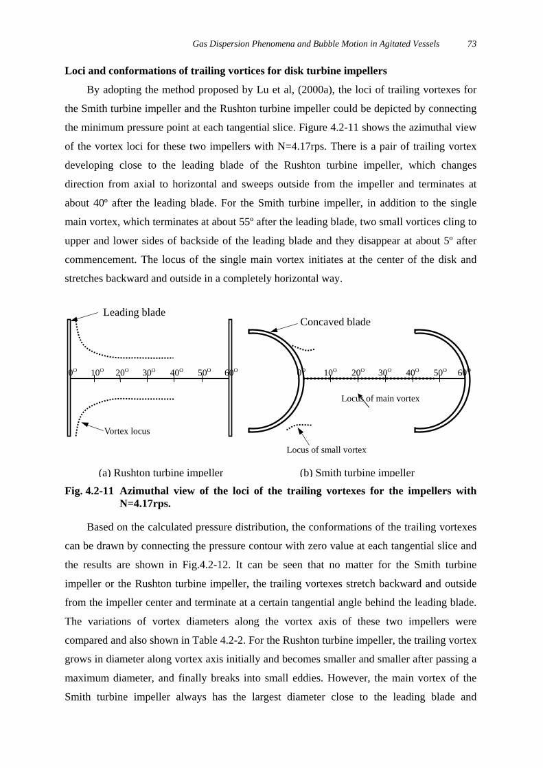
Loci and conformations of trailing vortices for disk turbine impellers
By adopting the method proposed by Lu et al, (2000a), the loci of trailing vortexes for
the Smith turbine impeller and the Rushton turbine impeller could be depicted by connecting
the minimum pressure point at each tangential slice. Figure 4.2-11 shows the azimuthal view
of the vortex loci for these two impellers with N=4.17rps. There is a pair of trailing vortex
developing close to the leading blade of the Rushton turbine impeller, which changes
direction from axial to horizontal and sweeps outside from the impeller and terminates at
about 40º after the leading blade. For the Smith turbine impeller, in addition to the single
main vortex, which terminates at about 55º after the leading blade, two small vortices cling to
upper and lower sides of backside of the leading blade and they disappear at about 5º after
commencement. The locus of the single main vortex initiates at the center of the disk and
stretches backward and outside in a completely horizontal way.
0O 10O 20O 30O 40O 50O 60O 0O 10O 20O 30O 40O 50O 60O
r
L e
Locus of main vortex
L x
C e
(a) Rushton turbine impeller (b) Smith turbine impelle
Fig. 4.2
Ba
can be d
the resu
impeller
from the
The var
compare
grows in
maximu
Smith t
Vortex locus
-1
s
r
l
i
d
m
u
eading blad
1 Azimuthal view of the loci of the N=4.17rps.
ed on the calculated pressure distribution,
awn by connecting the pressure contour w
ts are shown in Fig.4.2-12. It can be s
or the Rushton turbine impeller, the trail
impeller center and terminate at a certain
ations of vortex diameters along the v
and also shown in Table 4.2-2. For the R
diameter along vortex axis initially and b
diameter, and finally breaks into small
rbine impeller always has the largest
ocus of small vorte
tra
th
ith
een
ing
tan
ort
ush
eco
ed
dia
oncaved blad
iling vortexes for the impellers with
e conformations of the trailing vortexes
zero value at each tangential slice and
that no matter for the Smith turbine
vortexes stretch backward and outside
gential angle behind the leading blade.
ex axis of these two impellers were
ton turbine impeller, the trailing vortex
mes smaller and smaller after passing a
dies. However, the main vortex of the
meter close to the leading blade and

MULTIPLE IMPELLER GAS-LIQUID CONTACTORS74
continuously shrinks along the vortex axis and breaks into small eddies at the vortex tail.
Comparing the vortex sizes for these two impellers, it is found that the main vortex of the
Smith turbine impeller has a smaller maximum vortex diameter than the Rushton impeller
with a given rotational speed.
Fig
4.2
var
Fig
gra
mu
Main vortex
Small vortex
r
(a) Rushton turbine impeller (b) Smith turbine impelle. 4.2-12 Conformations of the trailing vortices for the Rushton turbine impeller andSmith turbine impeller with N=4.17rps.
.3 Mapping of ventilated cavities
By combining several relationship between rotational speed and gas flow rate for
ious cavity transition, Wannoeskerken et al.(1986) presented a flow map as shown in
.4.2-13. for the stirred vessel with flat blade disk turbine. This map enables an engineer to
sp the performance of gas dispersion. A very similar flow map as shown in Fig.4.2-14 for
ltiple impeller system was given by Smith et al. (1985).
Fig. 4.2-13 The flow map for the Rushton turbine (Warmoeskerken et al., 1986).

Gas Dispersion Phenomena and Bubble Motion in Agitated Vessels 75
Fig. 4.2-14 The flow map for multi-turbines vessel of T/D=2.5 (Smith,1985).
4.3 Machanism of Gas Dispersion behind Impeller Blades
To discuss the gas dispersion mechanisms of various impellers, the values of
deformation rates, shear stresses and the bubble size distribution at different locations around
the cavities should be estimated.
4.3.1 Forces related to gas dispersion around the trailing Vortex of Rushton turbine
The deformation rate and shear stress play important roles in gas dispersion. For the
cylindrical coordinates, the deformation rate tensor can be written as (Lu and Yang, 1998):
⎥⎥⎥⎥⎥⎥⎥
⎦
⎤
⎢⎢⎢⎢⎢⎢⎢
⎣
⎡
∂∂
∂∂
+∂∂
∂∂
+∂∂
∂∂
+∂∂
⎟⎠⎞
⎜⎝⎛ +
∂∂
∂∂
+⎟⎠⎞
⎜⎝⎛
∂∂
∂∂
+∂∂
∂∂
+⎟⎠⎞
⎜⎝⎛
∂∂
∂∂
=∆
zV2 1
zV
1z
V r12 1
rr
z
Vz
V 1r
r 2
z
rz
θ
θθθ
θ
θ
θθθ
θ
zrz
zrr
rr
Vrz
Vz
V
Vrr
VVVrr
V
Vrr
Vr
V
(4.3-1)
and the average deformation rate at each location can be calculated as:
∆∆= :21δ (4.3-2)
With the determined locus and conformation of trailing vortex (approximate to the vortex
cavity or clinging cavity), the forces related to gas dispersion were calculated and plotted
along the vortex axis. The deformation rates were calculated at the edge and central line of
the trailing vortex with N=4.17rps and the results were shown in Fig. 4.3-1. In this figure, Zv
denotes the position coordinate along the cavity axis and Zc is the full length of cavity axis,

MULTIPLE IMPELLER GAS-LIQUID CONTACTORS76
therefore the value of Zv/Zc is zero at the commencement of the vortex and equal to 1 at the
vortex tail (Van’t Riet and Smith, 1973). At the core of the trailing vortex, the deformation
rate increases monotonically along the vortex tail, while at edge of the vortex, it decreases
along with the vortex axis initially, after passing a minimum value at ZV/ZC=0.4, it increases
along with the vortex axis and gives a maximum value at vortex tail.
Fig. 4.3-1 Variation in deformation rate along the vortex axis at the core and edge ofthe trailing vortex with N=4.17rps.
Fig. 4.3-2 Variation in shear stress along the vortex axis at the core and edge of thetrailing vortex with N=4.17rps.
Similarly, the shear stress at each location was obtained by calculating the determinant
Gas Dispersion Phenomena and Bubble Motion in Agitated Vessels 77
of the following shear stress tensor.
⎥⎥⎥⎥⎥⎥⎥⎥
⎦
⎤
⎢⎢⎢⎢⎢⎢⎢⎢
⎣
⎡
⎥⎦⎤
⎢⎣⎡ ⋅∇−
∂∂
⎥⎦⎤
⎢⎣⎡
∂∂
+∂∂
⎥⎦⎤
⎢⎣⎡
∂∂
+∂∂
⎥⎦⎤
⎢⎣⎡
∂∂
+∂∂
⎥⎦⎤
⎢⎣⎡ ⋅∇−+
∂∂
⎥⎦
⎤⎢⎣
⎡∂∂
+⎟⎠⎞
⎜⎝⎛
∂∂
⎥⎦⎤
⎢⎣⎡
∂∂
+∂∂
⎥⎦
⎤⎢⎣
⎡∂∂
+⎟⎠⎞
⎜⎝⎛
∂∂
⎥⎦⎤
⎢⎣⎡ ⋅∇−
∂∂
=
)(32
zV2- 1
zV- -
1z
V- )(32)1(2- 1
r-
- 1r
- )(322-
z VVrz
Vz
V
Vr
Vr
VVr
Vrr
Vr
zV
zVV
rrVrV
rV
zrz
zrr
rzrr
µθ
µµ
θµ
θµ
θµ
µθ
µµ
τ
θ
θθθ
θ
(4-3-3)
And the results were compared for the circumference and central line of the trailing vortex as
shown in Fig. 4.3-2. It is found that (1) the largest shear stress always appears at vortex tail;
(2) a definite value of shear stress exists in the circumference of the vortex cavity, which
implies that the intense rotary motion happens to the vortex cavity or clinging cavity.
Yamamoto and Nishino (1992) had attempted to estimate the values of various dispersed
forces around the trailing vortex and the results were tabulated in Table 4.3-1 along with the
results obtained from this work. The measured mean bubble sizes at the circumference and
tail of the vortex cavity are also shown in this table for comparison. Both the results obtained
by Yamamoto and Nishino (1992) and this study show that: (1) the dispersing force resulting
from the turbulent eddy at the vortex tail was much larger than those provided by the rotary
motion of the vortex and the impeller blade itself; (2) the gas sucking force produced by the
negative pressure at the blade backside was the largest. Although all the results shown in this
table were obtained from the simulation for a single-phase systems, the structures of the
vortex and clinging cavities can be approximated. Therefore, it can be concluded that the
sparged gas was dispersed into small bubbles through two steps when the cavity structure
falls into the vortex or clinging cavities. First, gas is sucked into the vortex, and then
dispersed into small bubbles through the turbulent eddies around the vortex or turbulent eddy
at the vortex tail. Comparing the dispersed bubble sizes shown in this table, it was also found
that the bubbles appearing at the cavity tail result in a smaller mean bubble size.
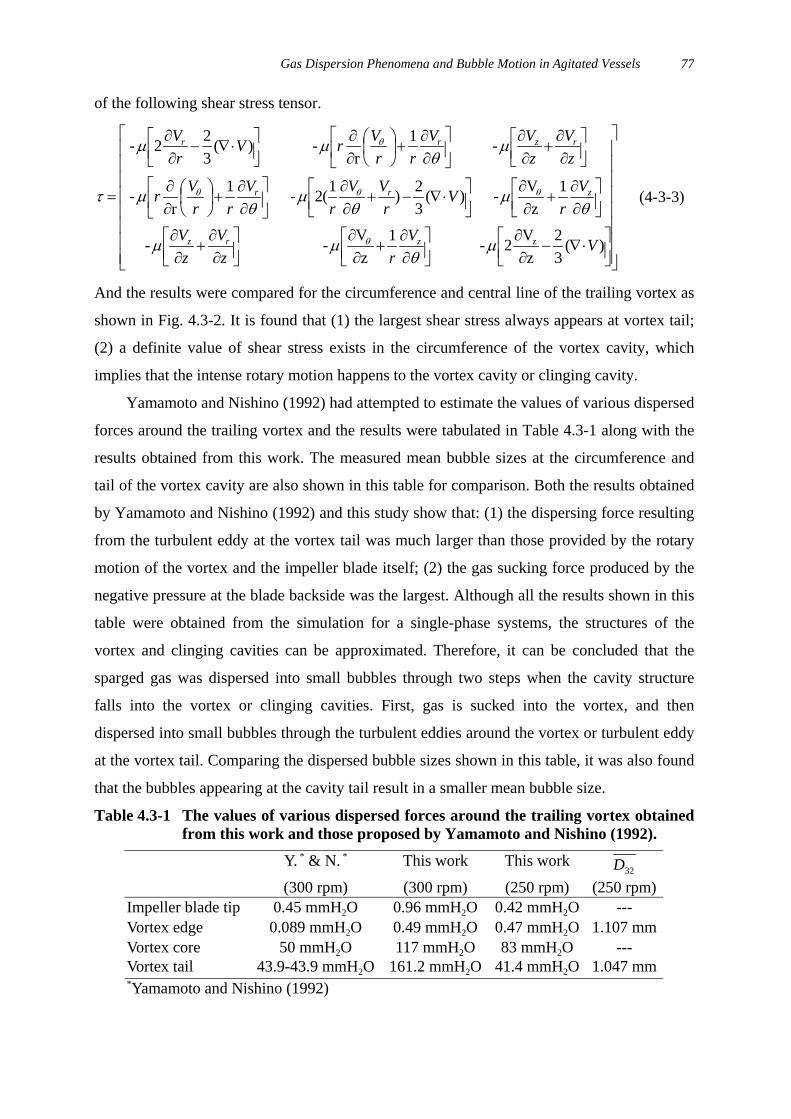
Table 4.3-1 The values of various dispersed forces around the trailing vortex obtainedfrom this work and those proposed by Yamamoto and Nishino (1992).
Y. * & N. * This work This work32D
(300 rpm) (300 rpm) (250 rpm) (250 rpm)Impeller blade tip 0.45 mmH2O 0.96 mmH2O 0.42 mmH2O ---Vortex edge 0.089 mmH2O 0.49 mmH2O 0.47 mmH2O 1.107 mmVortex core 50 mmH2O 117 mmH2O 83 mmH2O ---Vortex tail 43.9-43.9 mmH2O 161.2 mmH2O 41.4 mmH2O 1.047 mm*Yamamoto and Nishino (1992)
MULTIPLE IMPELLER GAS-LIQUID CONTACTORS78
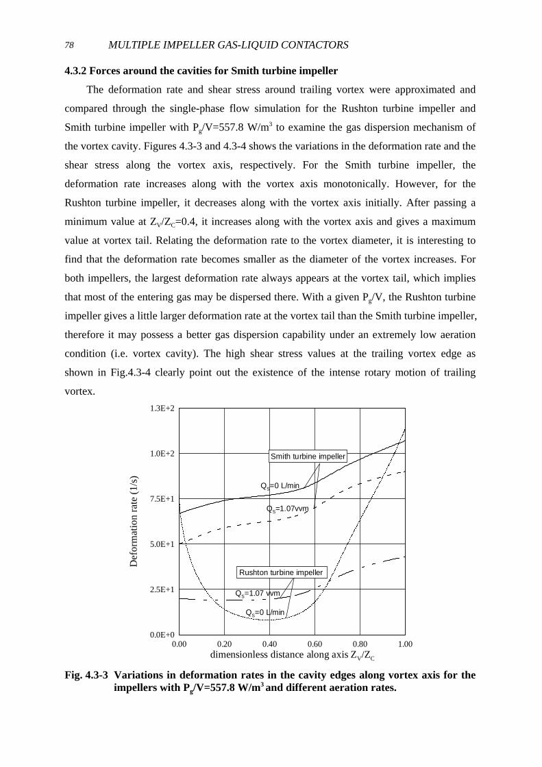
4.3.2 Forces around the cavities for Smith turbine impeller
The deformation rate and shear stress around trailing vortex were approximated and
compared through the single-phase flow simulation for the Rushton turbine impeller and
Smith turbine impeller with Pg/V=557.8 W/m3 to examine the gas dispersion mechanism of
the vortex cavity. Figures 4.3-3 and 4.3-4 shows the variations in the deformation rate and the
shear stress along the vortex axis, respectively. For the Smith turbine impeller, the
deformation rate increases along with the vortex axis monotonically. However, for the
Rushton turbine impeller, it decreases along with the vortex axis initially. After passing a
minimum value at ZV/ZC=0.4, it increases along with the vortex axis and gives a maximum
value at vortex tail. Relating the deformation rate to the vortex diameter, it is interesting to
find that the deformation rate becomes smaller as the diameter of the vortex increases. For
both impellers, the largest deformation rate always appears at the vortex tail, which implies
that most of the entering gas may be dispersed there. With a given Pg/V, the Rushton turbine
impeller gives a little larger deformation rate at the vortex tail than the Smith turbine impeller,
therefore it may possess a better gas dispersion capability under an extremely low aeration
condition (i.e. vortex cavity). The high shear stress values at the trailing vortex edge as
shown in Fig.4.3-4 clearly point out the existence of the intense rotary motion of trailing
vortex.
0.00 0.20 0.40 0.60 0.80 1.00dimensionless distance along axis ZV/ZC
0.0E+0
2.5E+1
5.0E+1
7.5E+1
1.0E+2
1.3E+2
Def
orm
atio
n ra
te (1
/s)
QS=0 L/min
QS=1.07vvm
QS=0 L/min
QS=1.07 vvm
Smith turbine impeller
Rushton turbine impeller
Fig. 4.3-3 Variations in deformation rates in the cavity edges along vortex axis for theimpellers with Pg/V=557.8 W/m3 and different aeration rates.

Gas Dispersion Phenomena and Bubble Motion in Agitated Vessels 79
Fig. 4.3-4 Variation in shear stresses in the cavity edges along vortex axis for theimpellers with Pg/V=557.8W/m3 and different aeration rates.
Adjusting the aeration rate QS to 1.07vvm and keep Pg/V as 557.8 W/m3, the cavity of
the Rushton turbine impeller has changed into the large cavity, while the vortex cavity still
clings to the Smith turbine impeller. The deformation rate and shear stress at the cavity edge
were calculated and the results are also shown in Fig.4.3-3 and Fig.4.3-4 to examine the gas
dispersion mechanisms of these two impellers under a higher aeration condition. For the
Rushton turbine impeller, once the cavity falls into the large cavity, the deformation rate
always increases smoothly with approaching the cavity tail and no minimum point exists in
the deformation rate curve as what is seen for the vortex cavity at ZV/ZC=0.4. Since the
maximum deformation rate at the tail of a large cavity is only approximately half of that for a
vortex cavity, the vortex cavity has a much better gas dispersion capability than the large
cavity. The large shear stress dose not appear at the periphery of a large cavity, which
indicates that the intense swirling motion does not exist for a large cavity any more and the
entering gas is dispersed at the tail of the large cavity only.
Comparing the deformation rate and shear stress for these two impellers with
QS=1.07vvm and Pg/V=557.8 W/m3, it is found that the Smith turbine impeller always gives
larger deformation rates and shear stresses. This fact demonstrates the better gas dispersion
capability of the Smith turbine impeller under a higher aeration condition. From the results
obtained here, one may conclude that no matter for the Smith turbine impeller or the Rushton
turbine impeller, the entering gas is mostly dispersed at either the tail and/or the
circumference of cavity through the larger shear force.
0.00 0.20 0.40 0.60 0.80 1.00dimensionless distance along axis ZV/ZC
0.0E+0
2.0E-7
4.0E-7
6.0E-7
8.0E-7
1.0E-6
1.2E-6
1.4E-6
1.6E-6
Shea
r stre
ss (k
g/m
s2 )
Rushton turbine impeller
Smith turbine impeller

MULTIPLE IMPELLER GAS-LIQUID CONTACTORS80
To examine the effect of the two small vortices appearing at the upper and lower edge of
leading blade of the Smith turbine impeller on the gas dispersion, the deformation rate and
shear stress around the small vortices are calculated under different operating conditions. It is
surprising to find out that the values of deformation rates and shear stress around the small
vortexes are guite large, even 30% higher than those at the tail of the cavity, which may
enhance the gas dispersion capability of the Smith turbine impeller.
4.3.3 Bubble size distributions around the cavity
Rushton turbine impeller
To illustrate how the forces related to the gas dispersion behind the blade, the bubble
sizes and bubble size distribution were experimentally determined at various locations around
different type cavities.
Fig. 4.3-5 The schematic diagram of the experimental setup and the distribution ofmeasured points for the bubble size measurements.
(a) Vortex core (b) Vortex tail (c) Vortex edge
Fig. 4.3-6 Distributions of bubble size at various locations around vortex cavity for thestandard Rushton turbine impeller with N=4.17rps and QS=0.8 L/min.
Gas Dispersion Phenomena and Bubble Motion in Agitated Vessels 81
(a) Vortex cavity
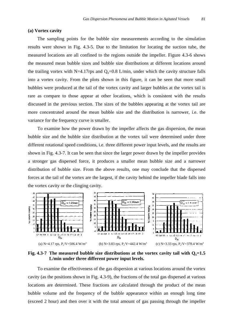
The sampling points for the bubble size measurements according to the simulation
results were shown in Fig. 4.3-5. Due to the limitation for locating the suction tube, the
measured locations are all confined to the regions outside the impeller. Figure 4.3-6 shows
the measured mean bubble sizes and bubble size distributions at different locations around
the trailing vortex with N=4.17rps and QS=0.8 L/min, under which the cavity structure falls
into a vortex cavity. From the plots shown in this figure, it can be seen that more small
bubbles were produced at the tail of the vortex cavity and larger bubbles at the vortex tail is
rare as compare to those appear at other locations, which is consistent with the results
discussed in the previous section. The sizes of the bubbles appearing at the vortex tail are
more concentrated around the mean bubble size and the distribution is narrower, i.e. the
variance for the frequency curve is smaller.
To examine how the power drawn by the impeller affects the gas dispersion, the mean
bubble size and the bubble size distribution at the vortex tail were determined under three
different rotational speed conditions, i.e. three different power input levels, and the results are
shown in Fig. 4.3-7. It can be seen that since the larger power drawn by the impeller provides
a stronger gas dispersed force, it produces a smaller mean bubble size and a narrower
distribution of bubble size. From the above results, one may conclude that the dispersed
forces at the tail of the vortex are the largest, if the cavity behind the impeller blade falls into
the vortex cavity or the clinging cavity.
(a) N=4.17 rps, Ps/V=506.4 W/m3 (b) N=3.83 rps, Ps/V=442.4 W/m3 (c) N=3.33 rps, Ps/V=378.4 W/m3
Fig. 4.3-7 The measured bubble size distributions at the vortex cavity tail with QS=1.5L/min under three different power input levels.
To examine the effectiveness of the gas dispersion at various locations around the vortex
cavity (as the positions shown in Fig. 4.3-9), the fractions of the total gas dispersed at various
locations are determined. These fractions are calculated through the product of the mean
bubble volume and the frequency of the bubble appearance within an enough long time
(exceed 2 hour) and then over it with the total amount of gas passing through the impeller

MULTIPLE IMPELLER GAS-LIQUID CONTACTORS82
(sum of the sparged and recirculated gas). Where the gas recirculation rate can be estimated
by using the method proposed by Lu et al. (2000). From the results shown in Table 4.3-2, it is
found that more than 60% of the total gas is dispersed at the vortex tail and approximately
15% is dispersed in the circumference of the trailing vortex. However, almost no gas is
dispersed at the vortex core, where gas is sucked into. This result quantitatively confirms the
conclusion which it was made in above.
Table 4.3-2 Comparison of the fraction of the sparged gas dispersed at the center,circumference and tail of the vortex under N=4.17rps and QS=0.8 L/min.
Position Vortex tail Vortex edge Vortex core Other placesFraction of the dispersed gas [%] 63.5 15.2 0.01 19.3
(b) Large cavity
Keep the cavity structure as a large cavity and change the rotational speed of impeller
and aeration rate into 6.67rps and QS=20.0 L/min=1.07vvm to give the same energy
dissipation density Pg/V=577.8 W/m3 as the vortex cavity. The mean bubble size and bubble
size distribution at the tail of a large cavity was determined and compared with that produced
at the tail of a vortex cavity as shown in Fig. 4.3-8. From the plots shown in this figure, it can
be seen that a large cavity produces much larger mean bubble size than that given by a vortex
cavity with the same energy dissipation density. This fact indicates that the capability of gas
dispersion of a large cavity is much worse than that of a vortex cavity.
(a) Large cavity (b) Vortex cavity
Fig. 4.3-8 Comparison of the bubble size distribution at the tail of a large cavity and avortex cavity with Pg/V=557.8W/m3.
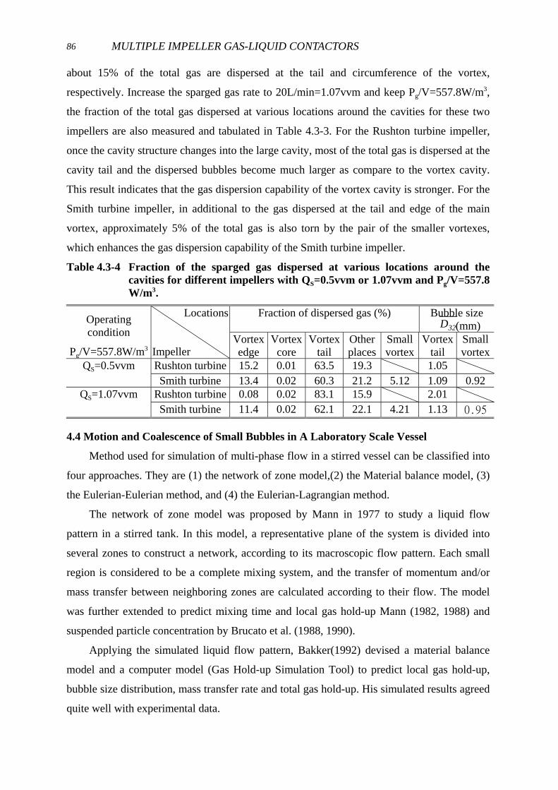
Similarly, the effectiveness of gas dispersion at various locations around a large cavity is
determined with a constant rotational speed as well as the same energy dissipation density as
the vortex cavity. The results are listed in Table 4.3-3 along with the gas dispersion fraction
obtained at the tail of a vortex cavity (N=4.17rps and QS=0.8L/min). It can be seen that no
Gas Dispersion Phenomena and Bubble Motion in Agitated Vessels 83
matter under what operating conditions, much more gas is dispersed at the tail of a large
cavity than that for a vortex cavity, which is more than 80% as compare to 60% for a vortex
cavity. However, almost no gas is dispersed at the edge of a large cavity, which clearly
indicates the diminution of the intense swirling motion of a large cavity.
Table 4.3-3 The fraction of the sparged gas dispersed at the center, circumference andtail of a large cavity with N=4.17rps and QS=20.0L/min along with thatobtained at the tail of a vortex cavity with N=4.17rps and QS=0.8L/min.
Large cavity Vortex tailPosition Tail Edge Core Other placesOperating conditions 4.17
[rps]0.35
[vvm]
557.8[W/m3]
1.07[vvm]
4.17[rps]
557.8[W/m3]
4.17[rps]
557.8[W/m3]
4.17[rps]
557.8[W/m3]
4.17[rps]
Fraction ofthe dispersed gas [%]
82.5 83.1 0.09 0.08 0.03 0.02 16.3 15.9 63.5
Effect of blade number on bubble size around the impellers
According to the observed conclusion reached by Takahashi and Nienow (1992) and
Barigou (1992), the bubbles near the location (r1, z2) or (r1, z4) are freshly generated and
underisturbed, therefore the discussion here will also concentrate on the values of bubble
diameters of determined at these points. Fig.4.3-9(a) and Fig.4.3-9(b) shows the size of
Sauter mean diameter of bubble diameter of bubbles around the impellers having 4, 6 and 8
blade under the same rotational speed of 4.17 rps or under the power input per each blade
respectively. Among the impellers having 4, 6 and 8 blades, the impeller with four blades has
not only the strongest mean deformation rates and the largest turbulent kinetics enemy, it also
has the smallest value of Sauter mean bubble diameter under a low gassing rate condition.The
next is the impeller with six blades. The impeller having eight blades performs the worst in
both cases. It is noticed that the bubbles appearing in the upper vortex are always smaller
than the bubbles dispersed by the lower vortex. This fact shows that the diameter of the upper
trailing vortex is usually smaller- (The size of vortex can be seen from the plot of mean
velocity in azimuthal planes, more details are available in Yang’s thesis (1995))-due to the
existence of hub on the upper side of tile impeller disk. Here, the impeller with two blades is
excluded from the discussion because the status of gas dispersion is different and a more
coalescent effect is possible involved due to low coverage of the vortex (lower value of the
ratio of azimuthal angle of the vortex to the azimuthal angle between two blades) as well as
the smaller pumping rate which makes it very difficult to obtain a good comparison.

MULTIPLE IMPELLER GAS-LIQUID CONTACTORS84
(a) (b)
Fig. 4.3-9(a) Comparison of 32D at r*=1.29 for various impellers with Qg=0.1L/min/blade and N=250 rpm.
(b) Comparison of D32 at *r =1.29 for various impellers with Qg=0.1L/min/blade and Pg=0.52 W/blade.
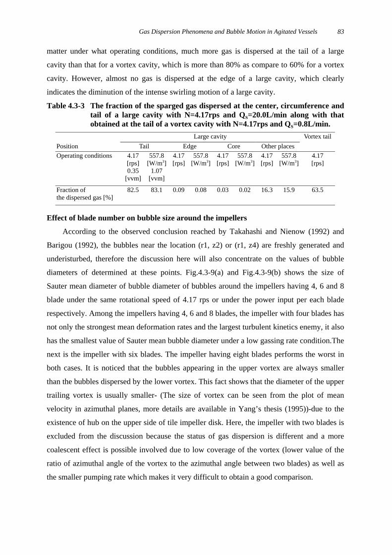
Comparison of the gas dispersion for different impellers
In accordance with the depicted conformations of the trailing vortices, the sizes of
dispersed bubbles at the core, edge and tail of the trailing vortices for the Rushton turbine
impeller and Smith turbine impeller were measured. Figure 4.3-10 shows the bubble size
distributions at the vortex tails around the Smith turbine impeller and Rushton turbine
impeller with QS=9.8L/min=0.5vvm and the same power input Pg/V=557.8 W/m3. Comparing
the plots shown in these two figures, one can find that the Rushton turbine impeller gives a
little smaller mean bubble size and result in a narrower bubble distribution about this mean
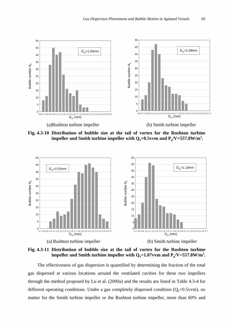
value. To accentuate the prevalence of the Smith turbine impeller under higher aeration
conditions, the bubble size and bubble size distributions for these two impellers were also
measured with QS=20L/min=1.07vvm and Pg/V=557.8 W/m3. Figure 4.3-11 compares the
measured bubble size distributions at the cavity tail for these two impellers with QS=1.07vvm
and Pg/V=557.8 W/m3. From the plots shown in this figure, one can see that the Smith turbine
impeller disperses gas more effectively under higher gassing rate condition and gives a much
smaller mean bubble size than the Rushton turbine impeller. The mean bubble size and
bubble size distribution around the small vortex attaching to the Smith turbine impeller are
also determined with QS=1.07vvm and Pg/V=557.8W/m3. It is found that the small vortexes
always result in much smaller bubbles ( mm95.0D32 = ) than those produced at other
locations. These results prove that the Smith turbine impeller possesses a better gas
dispersion capability and is proper to be used for the higher gassing condition.
Gas Dispersion Phenomena and Bubble Motion in Agitated Vessels 85
(a)Rushton turbine impeller (b) Smith turbine impeller
Fig. 4.3-10 Distribution of bubble size at the tail of vortex for the Rushton turbineimpeller and Smith turbine impeller with QS=0.5vvm and Pg/V=557.8W/m3.
(a) Rushton turbine impeller (b) Smith turbine impeller
Fig. 4.3-11 Distribution of bubble size at the tail of vortex for the Rushton turbineimpeller and Smith turbine impeller with QS=1.07vvm and Pg/V=557.8W/m3.
The effectiveness of gas dispersion is quantified by determining the fraction of the total
gas dispersed at various locations around the ventilated cavities for these two impellers
through the method proposed by Lu et al. (2000a) and the results are listed in Table 4.3-4 for
different operating conditions. Under a gas completely dispersed condition (QS=0.5vvm), no
matter for the Smith turbine impeller or the Rushton turbine impeller, more than 60% and
0.6 0.7 0.8 0.9 1.0 1.1 1.2 1.3 1.4 1.5 1.6 1.7 1.8 1.9 2.0 2.1 2.2 2.3 2.4 2.5 2.6 2.7
D32 (mm)
0
5
10
15
20
25
30
35
40
45
50
Bubb
le n
umbe
r Nb
D32=1.05mm
0.6 0.7 0.8 0.9 1.0 1.1 1.2 1.3 1.4 1.5 1.6 1.7 1.8 1.9 2.0 2.1 2.2 2.3 2.4 2.5 2.6 2.7
D32 (mm)
0
5
10
15
20
25
30
35
40
45
50
Bubb
le n
umbe
r Nb
D32=1.09mm
0.7 0.8 0.9 1.0 1.1 1.2 1.3 1.4 1.5 1.6 1.7 1.8 1.9 2.0 2.1 2.2 2.3 2.4 2.5 2.6 2.7
D32 (mm)
0
5
10
15
20
25
30
35
40
45
50
Bubb
le n
umbe
r Nb
D32=2.01mm
0.7 0.8 0.9 1.0 1.1 1.2 1.3 1.4 1.5 1.6 1.7 1.8 1.9 2.0 2.1 2.2 2.3 2.4 2.5 2.6 2.7
D32 (mm)
0
5
10
15
20
25
30
35
40
45
50
55
Bubb
le n
umbe
r Nb
D32=1.13mm
MULTIPLE IMPELLER GAS-LIQUID CONTACTORS86
about 15% of the total gas are dispersed at the tail and circumference of the vortex,
respectively. Increase the sparged gas rate to 20L/min=1.07vvm and keep Pg/V=557.8W/m3,
the fraction of the total gas dispersed at various locations around the cavities for these two
impellers are also measured and tabulated in Table 4.3-3. For the Rushton turbine impeller,
once the cavity structure changes into the large cavity, most of the total gas is dispersed at the
cavity tail and the dispersed bubbles become much larger as compare to the vortex cavity.
This result indicates that the gas dispersion capability of the vortex cavity is stronger. For the
Smith turbine impeller, in additional to the gas dispersed at the tail and edge of the main
vortex, approximately 5% of the total gas is also torn by the pair of the smaller vortexes,
which enhances the gas dispersion capability of the Smith turbine impeller.
Table 4.3-4 Fraction of the sparged gas dispersed at various locations around thecavities for different impellers with QS=0.5vvm or 1.07vvm and Pg/V=557.8W/m3.
Fraction of dispersed gas (%) Bubble size (mm)Operating
condition
Pg/V=557.8W/m3
Locations
ImpellerVortexedge
Vortexcore
Vortextail
Otherplaces
Smallvortex
Vortextail
Smallvortex
Rushton turbine 15.2 0.01 63.5 19.3 1.05QS=0.5vvmSmith turbine 13.4 0.02 60.3 21.2 5.12 1.09 0.92
Rushton turbine 0.08 0.02 83.1 15.9 2.01QS=1.07vvmSmith turbine 11.4 0.02 62.1 22.1 4.21 1.13 0.95
4.4 Motion and Coalescence of Small Bubbles in A Laboratory Scale Vessel
Method used for simulation of multi-phase flow in a stirred vessel can be classified into
four approaches. They are (1) the network of zone model,(2) the Material balance model, (3)
the Eulerian-Eulerian method, and (4) the Eulerian-Lagrangian method.
The network of zone model was proposed by Mann in 1977 to study a liquid flow
pattern in a stirred tank. In this model, a representative plane of the system is divided into
several zones to construct a network, according to its macroscopic flow pattern. Each small
region is considered to be a complete mixing system, and the transfer of momentum and/or
mass transfer between neighboring zones are calculated according to their flow. The model
was further extended to predict mixing time and local gas hold-up Mann (1982, 1988) and
suspended particle concentration by Brucato et al. (1988, 1990).
Applying the simulated liquid flow pattern, Bakker(1992) devised a material balance
model and a computer model (Gas Hold-up Simulation Tool) to predict local gas hold-up,
bubble size distribution, mass transfer rate and total gas hold-up. His simulated results agreed
quite well with experimental data.
32D

Gas Dispersion Phenomena and Bubble Motion in Agitated Vessels 87
The Eulerian-Eulerian approach was used by Issa and Gosman (1981) to study the
motion of gas and liquid in a stirred vessel. In their study, only a simplified momentum
equation of gas was considered. By considering turbulent phenomena, Looney et al. (1985)
estimated the locus of particle flow in a stirred vessel and had quite good results. Using the
Eulerian-Eulerian approach, it is possible to obtain the value of average velocity and the
turbulent characteristics of the dispersed phase in a stirred vessel system.
The Eulerian-Lagrangian method is the most popular approach used by researchers in
this field. Table 4.4-1 summarizes the results of studies using the E-L method in simulation
of multi-phase flow in stirred vessels. Patterson (1991) had discussed the effect of gas flow
on liquid flow, and has pointed out that liquid flow is not affected by the existence of gas
flow except when the gas flow rate is large. In this chapter, the E-L approach was adopted to
design a program to simulate the motion of small bubbles in a laboratory scale mechanically
stirred vessel with multiple impellers. The simple mechanism for coalescence and break-up
of bubbles is also considered in this simulation
Table4.4-1 Summary of results and boundary conditions in different E-L models.Zeitlin(1972) Ambeganontar(
1977)Fort et al.
(1986)Hutchings(1989
)Patterson(1991)
Dimension 2D 2D 2D 3D 3DNo. of dispersedparticle phase
Approximately1000
Multi-particles Multi-bubbles Single-bubblec=T/3
Multi-bubbles
No. and locationof impellers
Single stageturbine c=T/3
Single stageturbine c=T/3
Single stageturbine or A315c=T/3
Single stageturbine c=T/3
Single stageturbine c=T/3
Liquid flowimpeller
Tip velocity Seven regionanalytical solid
Eight zoneanalytical solid
Obtained byusing fluent
Obtained byusing fluent
Decision ofparticle velocity
See**
Coalescence Considered * Neglected Neglected NeglectedBreak up Considered * Neglected Neglected NeglectedFeed rate ofdispersed phase
Fixed gas hold-up
* Fixed gas flowrate
Fixed gas flowrate
Termination ofcalculation
Gas hold-up notchange
* Gas hold-up notchange
Objective results Local particleconcentration
Local particleconcentration
Local gas hold-up
Bubble motion Bubble motion
**:
Method to calculate Up
Zeitlen and Ambanontar Up =Uf +Ut, if random number ≧ U'/UUp =Ur, if random number ≦U'/U
Fort et al. Up =Uf +Ubax+Ur
Hutchings and Paterson Integrating force balance equation with respect to time

Gas Dispersion Phenomena and Bubble Motion in Agitated Vessels 73
4.4.1 Equation for motion of bubbles
For simplicity, it is assumed that the concentration of the bubbles in the mixing tank in
small. It can be assumed that the flow of the liquid is not affected by the presence of bubbles
and that interaction among bubbles is negligible. In addition, neither heat transfer nor mass
transfer is considered. Then, the motion of bubbles can be computed by considering a force
balance on the bubbles; i.e., the mass acceleration product is equal to the sum of the forces
acting on the bubble. The various forces acting on a bubble are as follows: (1) drag force, (2)
pressure gradient force, (3) buoyancy force, (4) added mass force, (5) Basset history force, (6)
lift force, and (7) wall force presented by Antal et al. (1991). Then, the equation of motion for
a bubble having mass M moving at velocity Vb, in a liquid with velocity UL can be expressed
as follows (Chiu, 1994):
)(''
)()(1)()23(
)()()()()43(
021
2
'0
2
yRCC
RUm
UVUmCdtttdt
VUdCdm
dtdV
dtdUmCgmMU
DtDUmUVVVC
dm
dtdVM
bWW
bLbLL
tbLL
n
bLVLL
LLbLbd
b
++×∇⋅−+−
−+
−+−+∇−+−−−=
∫πν
ν
(4.4-1)
where Cd, the drag coefficient, is estimated from universal correlations of the bubble rise
speed in a large extent of liquid following Wallis (1974). The liquid velocity is given by UL =
uL+u’L, where uL is obtained from the mean flow of liquid calculated by FLUENT, u’L is
chosen randomly from an isotropic Gaussian distribution with mean square deviation 2κ/3,
and κis the turbulent kinetic energy of the liquid estimated by FLUENT. The bubble
location at any instant of time is given by dXb/dt =Vb.
4.4.2 Bubble diameter in the pressure field
If it is assumed that the bubble is spherical and the mass and heat transfer between the
two phases are not considered, then the change of bubble diameter can be considered in a
quasi-steady-state. The equation of the change of bubble diameter in terms of the pressure
difference, ambient static pressure of the liquid and the internal pressure of the bubble can be
given as (Chiu, 1994):
(p-pv) d3+4σd3-podo3=0 (4.4-2)
where the liquid ambient static pressure p can be estimated as a function of position, pv, po, do
denote the saturated vapor pressure, the initial values of the pressure in the bubble and the
initial bubble diameter, respectively.
4.4.3 Mechanism of bubble coalescence
The coalescence of a pair of bubbles was found to consist of the following three
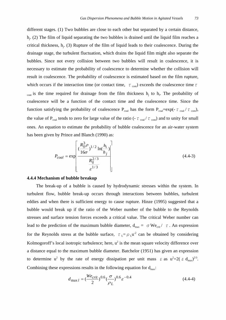
Gas Dispersion Phenomena and Bubble Motion in Agitated Vessels 73
different stages. (1) Two bubbles are close to each other but separated by a certain distance,
hj. (2) The film of liquid separating the two bubbles is drained until the liquid film reaches a
critical thickness, hj. (3) Rupture of the film of liquid leads to their coalescence. During the
drainage stage, the turbulent fluctuation, which drains the liquid film might also separate the
bubbles. Since not every collision between two bubbles will result in coalescence, it is
necessary to estimate the probability of coalescence to determine whether the collision will
result in coalescence. The probability of coalescence is estimated based on the film rupture,
which occurs if the interaction time (or contact time, τcont) exceeds the coalescence timeτ
cont is the time required for drainage from the film thickness hj to hf. The probability of
coalescence will be a function of the contact time and the coalescence time. Since the
function satisfying the probability of coalescence Pcoal has the form Pcoal=exp(-τcoal /τcont),
the value of Pcoal tends to zero for large value of the ratio (-τcoal /τcont) and to unity for small
ones. An equation to estimate the probability of bubble coalescence for an air-water system
has been given by Prince and Blanch (1990) as:
⎥⎥⎥⎥⎥⎥
⎦
⎤
⎢⎢⎢⎢⎢⎢
⎣
⎡
=
3/1
3/2
2/13
)ln()16
(exp
ε
σ
ρ
ij
j
iij
coalR
hhR
P (4.4-3)
4.4.4 Mechanism of bubble breakup
The break-up of a bubble is caused by hydrodynamic stresses within the system. In
turbulent flow, bubble break-up occurs through interactions between bubbles, turbulent
eddies and when there is sufficient energy to cause rupture. Hinze (1995) suggested that a
bubble would break up if the ratio of the Weber number of the bubble to the Reynolds
stresses and surface tension forces exceeds a critical value. The critical Weber number can
lead to the prediction of the maximum bubble diameter, dmax = σWecrit / τ. An expression
for the Reynolds stress at the bubble surface, τL=ρLu-2 can be obtained by considering
Kolmogoroff’s local isotropic turbulence; here, u2 is the mean square velocity difference over
a distance equal to the maximum bubble diameter. Batchelor (1951) has given an expression
to determine u2 by the rate of energy dissipation per unit mass εas u2=2(εdmax)2/3.
Combining these expressions results in the following equation for dmax:
4.06.06.0max )()
2( −= ε
ρσ
L
critl
Wed (4.4-4)
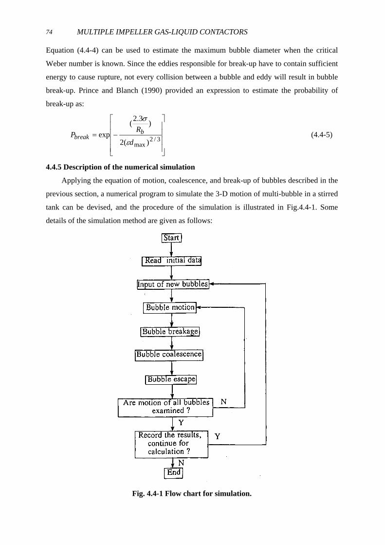
MULTIPLE IMPELLER GAS-LIQUID CONTACTORS74
Equation (4.4-4) can be used to estimate the maximum bubble diameter when the critical
Weber number is known. Since the eddies responsible for break-up have to contain sufficient
energy to cause rupture, not every collision between a bubble and eddy will result in bubble
break-up. Prince and Blanch (1990) provided an expression to estimate the probability of
break-up as:
⎥⎥⎥⎥
⎦
⎤
⎢⎢⎢⎢
⎣
⎡
−= 3/2max )(2
)3.2(exp
d
RP b
breakε
σ
(4.4-5)
4.4.5 Description of the numerical simulation
Applying the equation of motion, coalescence, and break-up of bubbles described in the
previous section, a numerical program to simulate the 3-D motion of multi-bubble in a stirred
tank can be devised, and the procedure of the simulation is illustrated in Fig.4.4-1. Some
details of the simulation method are given as follows:
Fig. 4.4-1 Flow chart for simulation.
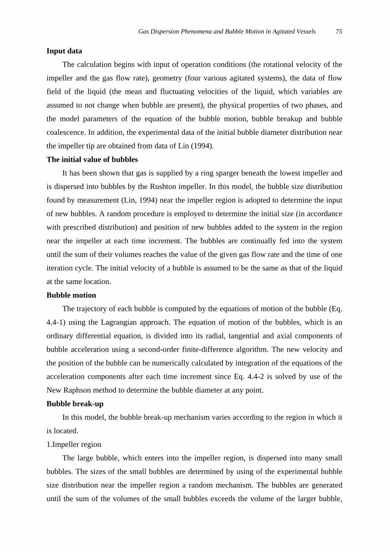
Gas Dispersion Phenomena and Bubble Motion in Agitated Vessels 75
Input data
The calculation begins with input of operation conditions (the rotational velocity of the
impeller and the gas flow rate), geometry (four various agitated systems), the data of flow
field of the liquid (the mean and fluctuating velocities of the liquid, which variables are
assumed to not change when bubble are present), the physical properties of two phases, and
the model parameters of the equation of the bubble motion, bubble breakup and bubble
coalescence. In addition, the experimental data of the initial bubble diameter distribution near
the impeller tip are obtained from data of Lin (1994).
The initial value of bubbles
It has been shown that gas is supplied by a ring sparger beneath the lowest impeller and
is dispersed into bubbles by the Rushton impeller. In this model, the bubble size distribution
found by measurement (Lin, 1994) near the impeller region is adopted to determine the input
of new bubbles. A random procedure is employed to determine the initial size (in accordance
with prescribed distribution) and position of new bubbles added to the system in the region
near the impeller at each time increment. The bubbles are continually fed into the system
until the sum of their volumes reaches the value of the given gas flow rate and the time of one
iteration cycle. The initial velocity of a bubble is assumed to be the same as that of the liquid
at the same location.
Bubble motion
The trajectory of each bubble is computed by the equations of motion of the bubble (Eq.
4.4-1) using the Lagrangian approach. The equation of motion of the bubbles, which is an
ordinary differential equation, is divided into its radial, tangential and axial components of
bubble acceleration using a second-order finite-difference algorithm. The new velocity and
the position of the bubble can be numerically calculated by integration of the equations of the
acceleration components after each time increment since Eq. 4.4-2 is solved by use of the
New Raphson method to determine the bubble diameter at any point.
Bubble break-up
In this model, the bubble break-up mechanism varies according to the region in which it
is located.
1. Impeller region
The large bubble, which enters into the impeller region, is dispersed into many small
bubbles. The sizes of the small bubbles are determined by using of the experimental bubble
size distribution near the impeller region a random mechanism. The bubbles are generated
until the sum of the volumes of the small bubbles exceeds the volume of the larger bubble,

MULTIPLE IMPELLER GAS-LIQUID CONTACTORS76
which was dispersed.
2. Bulk region
When the size of the bubble is near the maximum bubble size, a random procedure is
used to determine whether the bubble will break according to the probability of bubble break-
up. If bubble breakage occurs, the bubble is assumed to break into two small ones of equal
size. No breakage occurs when the size of the bubble is smaller than the maximum bubble
size.
Bubble coalescence
If a bubble collides with another bubble, a random procedure is used to determine the
probability of whether the collision will result in bubble coalescence.
Escape of bubbles
If a bubble moves through the liquid to the free surface, the bubble is assumed to leave
the system.
Output data
The program continues to calculate the bubble motion after another bubble is examined.
After the motion of all the bubbles at this iteration are examined, the program records the
results and decides whether to continue or terminate the simulations. If the program decides
to continue, it returns to the stage of input of new bubbles.
4.4.6 Simulated bubble motion and its effect on power consumption of the impellers
To examine the effect of the motion of bubbles within the system on the power
consumption of each impeller in multiple impeller systems, simulation of bubble motion was
carried out for four different geometrical systems as described in part I and shown in Table
4.4-2. Differential gas flow rates were also imposed to determine how the gas flow rate
would affect the bubble size, which is caused by the coalescence and break-up of the bubble.
In Fig. 4.4-2, variations of bubble size with time for various tank designs and various
flow rates are shown. The average size of bubbles increases with time due to coalescence of
bubbles. Comparing curves (4), (3) and (2) it can be seen that the gas flow rate clearly affects
the size of bubbles because the increase in the gas flow rate naturally enhances the chance of
coalescence of bubbles. From a comparison of curves (4) and (5) no significant difference in
average bubble size is observed between the systems of the dual and the triple Rushton
turbine. Although greater liquid depth and longer retention time should cause more
coalescence, the additional stage of impeller redisperses the sucked gas and break-up some of
larger bubble. Finally, it results in only a slight difference is seen in the average size of
bubbles. Comparing curves (3) and (6), the effect of the different flow patterns on the growth
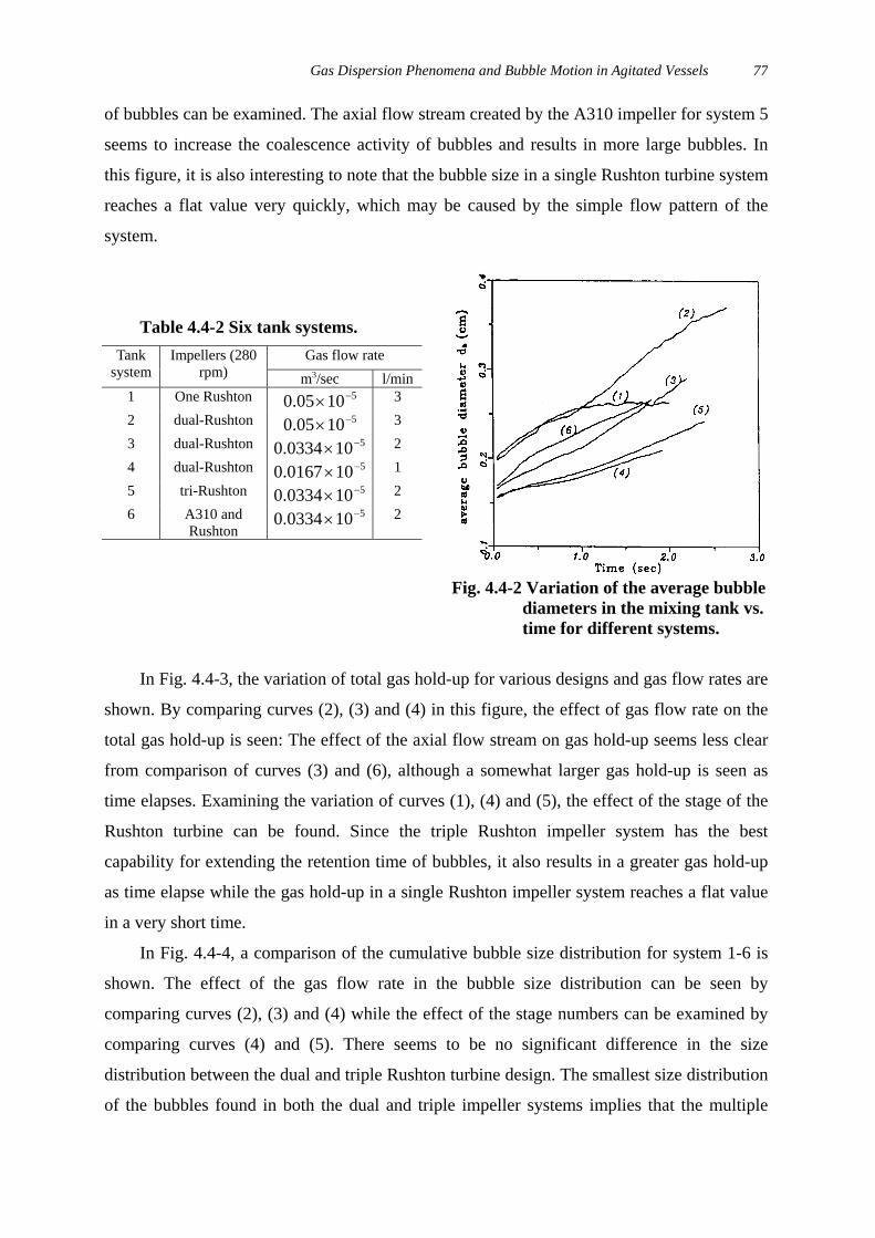
Gas Dispersion Phenomena and Bubble Motion in Agitated Vessels 77
of bubbles can be examined. The axial flow stream created by the A310 impeller for system 5
seems to increase the coalescence activity of bubbles and results in more large bubbles. In
this figure, it is also interesting to note that the bubble size in a single Rushton turbine system
reaches a flat value very quickly, which may be caused by the simple flow pattern of the
system.
Table 4.4-2 Six tank systems.Gas flow rateTank
systemImpellers (280
rpm) m3/sec l/min1 One Rushton 51005.0 −× 32 dual-Rushton 51005.0 −× 33 dual-Rushton 5100334.0 −× 24 dual-Rushton 5100167.0 −× 15 tri-Rushton 5100334.0 −× 26 A310 and
Rushton5100334.0 −× 2
Fig. 4.4-2 Variation of the average bubblediameters in the mixing tank vs.time for different systems.
In Fig. 4.4-3, the variation of total gas hold-up for various designs and gas flow rates are
shown. By comparing curves (2), (3) and (4) in this figure, the effect of gas flow rate on the
total gas hold-up is seen: The effect of the axial flow stream on gas hold-up seems less clear
from comparison of curves (3) and (6), although a somewhat larger gas hold-up is seen as
time elapses. Examining the variation of curves (1), (4) and (5), the effect of the stage of the
Rushton turbine can be found. Since the triple Rushton impeller system has the best
capability for extending the retention time of bubbles, it also results in a greater gas hold-up
as time elapse while the gas hold-up in a single Rushton impeller system reaches a flat value
in a very short time.
In Fig. 4.4-4, a comparison of the cumulative bubble size distribution for system 1-6 is
shown. The effect of the gas flow rate in the bubble size distribution can be seen by
comparing curves (2), (3) and (4) while the effect of the stage numbers can be examined by
comparing curves (4) and (5). There seems to be no significant difference in the size
distribution between the dual and triple Rushton turbine design. The smallest size distribution
of the bubbles found in both the dual and triple impeller systems implies that the multiple
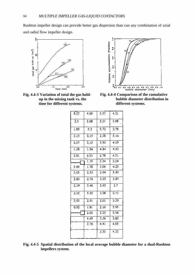
MULTIPLE IMPELLER GAS-LIQUID CONTACTORS94
Rushton impeller design can provide better gas dispersion than can any combination of axial
and radial flow impeller design.
Fig. 4.4-3 Variation of total the gas hold-up in the mixing tank vs. thetime for different systems.
Fig. 4.4-4 Comparison of the cumulativebubble diameter distribution indifferent systems.
Fig. 4.4-5 Spatial distribution of the local average bubble diameter for a dual-Rushtonimpellers system.

Gas Dispersion Phenomena and Bubble Motion in Agitated Vessels 95
Fig. 4.4-5 illustrates the spatial distribution of local average bubble diameter for the
system with dual Rushton turbines. The simulated result clearly shows that the local bubble
diameter is heavily dependent on the local strength of the turbulent and flow pattern. The
smallest bubbles are found near the impeller discharge region and the center core of the
vessel. Larger bubbles are found near the wall and baffle plates due to the greater opportunity
for coalescence in these regions. The bubble size increases along the discharge stream
because the turbulent eddies of the discharge flow enhance coalescence.
In Fig. 4.4-6 comparisons between simulated mean bubble sizes at discharge region in
system 1 and system 2 are presented. Although the values are not quite the same, the order
and the magnitude are in acceptable deviation.System 1
System 2
Fig. 4.4-6 Comparison between simulated 32D and experimental 32D .
Fig. 4.4-7(a), 4.4-7(b) and 4.4-7(c) show examples of bubble distribution for system 2
(Dual Rushton Turbines) at three different vertical planes, i.e., at the 45° mid-plane, the
plane in front of the baffle (relative to the fluid flow direction) and the plane behind the baffle.
Figure 4.4-8(a) (b) and (c) show the similar picture for the system 5, which was triple
Rushton Turbine. These pictures clearly demonstrate that the bubble distribution of the tank

MULTIPLE IMPELLER GAS-LIQUID CONTACTORS96
is far from homogeneous. Most bubbles were driven very quickly to the wall due to the high
radial velocity of the impeller discharge stream. From picture Fig. 4.4-7(b) and 4.4-8(b) it can
be seen that bubbles in front of the baffle plates tend to collide with each other, become
larger bubbles and rise along the baffle plates while bubbles at other planes tend to recirculate
along the fluid flow in the tank.
(a) (b) (c)
Fig. 4.4-7 Diagram of the bubbles in the stirred tank with a dual Rushton impellerssystem(gas flow rate =3 l /min, rotational speed =250 rpm).(a) Midway between the baffles(b) In front of the baffles(c) Behind the baffles
(a) (b) (c)
Fig. 4.4-8 Diagram of bubbles in a triple impeller system (Qg=1 l/min, N=250 rpm).
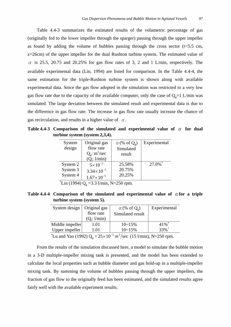
Gas Dispersion Phenomena and Bubble Motion in Agitated Vessels 97
Table 4.4-3 summarizes the estimated results of the volumetric percentage of gas
(originally fed to the lower impeller through the sparger) passing through the upper impeller
as found by adding the volume of bubbles passing through the cross sector (r<5.5 cm,
z=26cm) of the upper impeller for the dual Rushton turbine system. The estimated value of
α is 25.5, 20.75 and 20.25% for gas flow rates of 3, 2 and 1 L/min, respectively. The
available experimental data (Lin, 1994) are listed for comparison. In the Table 4.4-4, the
same estimation for the triple-Rushton turbine system is shown along with available
experimental data. Since the gas flow adopted in the simulation was restricted to a very low
gas flow rate due to the capacity of the available computer, only the case of Qg=1 L/min was
simulated. The large deviation between the simulated result and experimental data is due to
the difference in gas flow rate. The increase in gas flow rate usually increase the chance of
gas recirculation, and results in a higher value of α.
Table 4.4-3 Comparison of the simulated and experimental value of α for dualturbine system (system 2,3,4).
Systemdesign
Original gasflow rate
Qg: m3/sec(Ql: l/min)
α(% of Qg)Simulated
result
Experimental
System 2System 3System 4
5105 −×51034.3 −×51067.1 −×
25.58%20.75%20.25%
27.0%*
*Lin (1994) Qg =3.3 l/min, N=250 rpm.
Table 4.4-4 Comparison of the simulated and experimental value of αfor a tripleturbine system (system 5).
System design Original gasflow rate
(Ql: l/min)
α(% of Qg)Simulated result
Experimental
Middle impellerUpper impeller
1.011.01
10~15%10~15%
41%*
33%*
*Lu and Yao (1992) Qg = sec1025 35 m−× (15 l/min), N=250 rpm.
From the results of the simulation discussed here, a model to simulate the bubble motion
in a 3-D multiple-impeller mixing tank is presented, and the model has been extended to
calculate the local properties such as bubble diameter and gas hold-up in a multiple-impeller
mixing tank. By summing the volume of bubbles passing through the upper impellers, the
fraction of gas flow to the originally feed has been estimated, and the simulated results agree
fairly well with the available experiment results.
MULTIPLE IMPELLER GAS-LIQUID CONTACTORS98
NOTATION
B Baffle width [m]
D Impeller diameter [m]
Di Bubble size for each measurement point [m]
D32 Sauter mean bubble diameter [m]
Fl Gas flow number(=Qg/ND3) [-]
Fr Froud number [-]
g Gravitation factor [m/s2]
H Liquid level of stirred tank [m]
h0 Height of lower impeller from bottom [m]
k Dimensionless turbulent kinetic energy [-]
L Turbulence macroscale [m]
Lres Resultant turbulence scale [m]
N Impeller rotational speed [1/s]
NA Aeration number(=Q/ND3) [-]
Nc Transitional impeller rotating speed for stage(c) to stage(d) in Fig.3.2-1 [s-1]
NF Impeller rotating speed at flooding point [s-1]
No Minimum impeller speed which can disperse gas completely [s-1]
Nc Transitional impeller rotating speed for stage(d) to stage(f) in Fig.3.2-1 [s-1]
nb Baffle number [-]
nI Impeller number [-]
np Number of impeller blade [-]
P Power consumption [W]
P0 The ambient pressure for the cavity [kg/s2m2]
Pg Power consumption with aeration [kgm2/s3]
Po Power consumption without aeration [kgm2/s3]
QS Sparged gas flow rate [m3/s]
qi,l,g Liquid volumetric flow rate between cells in the I direction [m3/s]
r Radial coordinate [m]
r* Dimensionless radial coordinate(=2r/D) [-]
s Time [s]
T Tank diameter [m]
tM Mixing time [s]
U Rotating frame of reference mean velocity [m/s]
Ul,g Liquid phase velocity with aeration [m/s]
Ul,u Liquid phase velocity without aeration [m/s]
u’,v’ Fluctuation velocity [m/s]
V Liquid volume in the tank [m3]
v Stationary frame of reference mean velocity [m/s]
Vtip Impeller tip velocity [m/s]
W Mean tangential velocity [m/s]
w Impeller blade width [m]
Z Axial coordinate [m]
Gas Dispersion Phenomena and Bubble Motion in Agitated Vessels 99
z* Dimensionless axial coordinate(=2z/w) [-]
<Greeks Letters>Δ Mean rate of deformation tensor [1/s]
α Defined in Eq.(6-1)(=nbB/T) [-]
β Exponent adopted in Eq.(6.1-2) [-]
δ Mean deformation rate [1/s]
ε Energy dispersion rate [m2/s3]
εg Local gas hold-up [-]
θ Shaft angular position [degree]
κ Turbulent kinetic energy [m2/s2]
ρ Density [kg/m3]
σ Surface tension [N/m]
ω Mean rotation rate [1/s]
<Subscripts>cd Completely dispersed condition
g Gassed condition
i Initial condition
l Liquid phase
Pro Projective
r,θ,z Radial, tangential, axial
u Ungassed condition
∞ Final condition
<Superscripts>* Nondimensional
- Average quantity
~ Instantaneous quantity