Embed Size (px)
Citation preview
GAS BUILD-UP IN A DOMESTIC PROPERTY FOLLOWING
RELEASES OF METHANE/HYDROGEN MIXTURES
Lowesmith, B.J.1 , Hankinson, G.
1, Spataru, C.
l and Stobbart, M.
2
1 Chem. Eng. Dept, Loughborough University, Loughborough, LE11 3TU, UK 2 Advantica Ltd, Spadeadam Test Site, Spadeadam, Cumbria, CA8 7AU, UK
ABSTRACT
The EC funded Naturalhy project is investigating the possibility of promoting the swift introduction of
hydrogen as a fuel, by mixing hydrogen with natural gas and transporting this mixture by means of the
existing natural gas pipeline system to end-users. Hydrogen may then be extracted for use in
hydrogen fuel cell applications or the mixture may be used directly in conventional gas-fired
equipment. This means that domestic customers would receive a natural gas (methane)/hydrogen
mixture delivered to the home. As the characteristics of hydrogen are different from natural gas, there
may be an increased risk to end-users in the event of an accidental release of gas from internal pipe
work or appliances. Consequently, part of the Naturalhy project is aimed at assessing the potential
implications on the safety of the public, which includes end-users in their homes. In order to
understand the nature of any gas accumulation which may form and identify the controlling
parameters, a series of large scale experiments have been performed to study gas accumulations within
a 3 m by 3 m by 2.3 m ventilated enclosure representing a domestic room. Gas was released vertically
upwards at a pressure typical of that experienced in a domestic environment from hole sizes
representative of leaks and breaks in pipe work. The released gas composition was varied and
included methane and a range of methane/hydrogen mixtures containing up to 50% hydrogen. During
the experiments gas concentrations throughout the enclosure and the external wind conditions were
monitored with time. The experimental data is presented. Analysis of the data and predictions using a
model developed to interpret the experimental data show that both buoyancy and wind driven
ventilation are important.
1.0 BACKGROUND
Hydrogen is seen as an important energy carrier for the future which offers carbon free emissions at
the point of use. However, transition to the hydrogen economy is likely to be lengthy and will take
considerable investment with major changes to the technologies required for the manufacture,
transport and use of hydrogen. In order to facilitate the transition to the hydrogen economy, the EC
funded project Naturalhy is studying the potential for the existing natural gas pipeline networks to
transport hydrogen from manufacturing sites to hydrogen users. The hydrogen, introduced into the
pipeline network, would mix with the natural gas. This mixture could then be used directly by
consumers as a fuel within existing gas powered equipment, with the benefit of lower carbon
emissions. In addition, hydrogen could be extracted from the mixture for use in hydrogen powered
engines or for hydrogen fuel cell applications. Using the existing pipeline network to convey
hydrogen in this way, would enable hydrogen production and hydrogen fuelled applications to become
established prior to the development of a dedicated hydrogen transportation system, which would
require considerable capital investment and time for construction.
However, the existing gas pipeline networks are designed, constructed and operated based on the
premise that natural gas is the material to be conveyed. Hydrogen has different chemical and physical
properties which may adversely affect the integrity or durability of the pipeline network, or which may
increase the risk presented to the public. For these reasons, the Naturalhy project has been initiated to
assess the feasibility and impact of introducing hydrogen into a natural gas pipeline system.
Determining any change in risk to the public is a major part of this project. For example, although
rare, escapes of gas from faulty appliances or joints in internal pipe work do occur and sometimes
result in the formation of a flammable accumulation. Each year, a small number of such escapes result
in an explosion with the potential to harm the occupants and cause damage to the building. The
introduction of hydrogen into the supplied gas may increase the risk of such explosions due to the
change in way in which the gas accumulation forms and/or due to the increased reactivity of hydrogen.
In order to understand the nature of any accumulation of natural gas/hydrogen which may form and to
identify the controlling parameters, a series of large scale experiments have been undertaken in which
methane/hydrogen mixtures were released within a room-sized enclosure under conditions which are
typical of a domestic environment. Assessment of the data enabled identification of the controlling
parameters and aided the development and validation of a mathematical model.
2.0 INTRODUCTION
The concentration and extent of the flammable accumulation will affect the severity of the resulting
explosion and hence it is important to understand the controlling parameters of gas build-up
behaviour. For natural gas, the characteristics of gas escapes in the home are well understood. For
example, gas accumulations will tend to form a layer of uniform concentration in that part of the room
above the height of the release point. Factors which contribute to this behaviour are: the low
momentum of gas release (due to the typical gas pressure being 20-30 mbar); the density of natural gas
being less than that of air; and the generally low velocity of airflow (ventilation) within domestic
buildings.
However, natural gas/hydrogen mixtures have a lower density than natural gas and this may give rise
to different gas accumulation behaviour. Also, for a given supply pressure and leak size, the volume
flow rate of natural gas/hydrogen will be greater than the equivalent leak involving methane. Hence, it
might be expected that the resulting gas concentration will be higher. Furthermore, due to the wide
flammability limits of the mixture, a larger flammable volume may result. In order to assess any
change in gas accumulation behaviour, the large scale experiments reported here studied gas releases
at pressures typical of that found in a domestic building from leak sizes typical of those that may
occur, involving methane (representing natural gas) and methane/hydrogen mixtures. As a flammable
concentration will be reached more readily if the escape results in an accumulation in only part of the
room (a ‘layer’) this represents the more hazardous situation. Hence, the experimental programme was
designed such that most tests involved a gas release which was vertically upwards from a location at
half-height. Furthermore, the ventilation regime was such that air would enter the room at low level
and gas mixture leave the room at high level. This situation promoted the formation of a ‘layer’ in the
upper part of the room.
3.0 EXPERIMENTAL DETAILS
3.1 Experimental Arrangement
The experiments were conducted at the Advantica Limited test site at Spadeadam in the north of
England. The test rig was designed to represent a typical domestic room and consequently measured 3
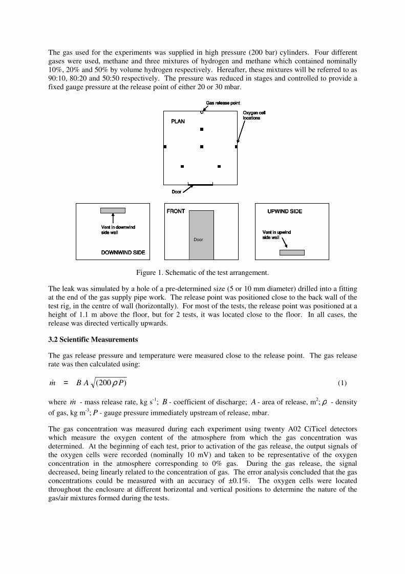
m by 3 m by 2.3 m high. Figure 1 shows a schematic of the test arrangement. In one wall of the test
rig (front wall) a lightweight door (typical of that used inside a domestic property) was installed
measuring 0.9 m by 2 m high. This was located within a typical door frame and a door jamb nailed to
the doorframe to hold the door in place. The arrangement was therefore characteristic of the situation
where the door opens into the room. The two side walls, each adjacent to the front wall, incorporated
ventilation openings which could be adjusted in size and could provide a well-defined ventilation
pattern to the enclosure. The upwind side wall (facing the wind) had an opening at low level, located
200 mm above the floor. The downwind side had an opening the same size at high level, 200mm
below the ceiling. Each ventilation opening measured 1 m in the horizontal direction and was adjusted
in size in the vertical direction. The back wall, floor and ceiling were plain and incorporated no
fittings.
The gas used for the experiments was supplied in high pressure (200 bar) cylinders. Four different
gases were used, methane and three mixtures of hydrogen and methane which contained nominally
10%, 20% and 50% by volume hydrogen respectively. Hereafter, these mixtures will be referred to as
90:10, 80:20 and 50:50 respectively. The pressure was reduced in stages and controlled to provide a
fixed gauge pressure at the release point of either 20 or 30 mbar.
Gas release point
PLAN
Oxygen cell
locations
Door
FRONT
Vent in upwind
side wall
UPWIND SIDE
Vent in downwind
side wall
DOWNWIND SIDE
Door
Gas release point
PLAN
Oxygen cell
locations
Door
FRONT
Vent in upwind
side wall
UPWIND SIDE
Vent in downwind
side wall
DOWNWIND SIDE
Gas release point
PLAN
Oxygen cell
locations
Door
FRONT
Vent in upwind
side wall
UPWIND SIDE
Gas release point
PLAN
Oxygen cell
locations
Door
Gas release point
PLAN
Oxygen cell
locations
Door
FRONTFRONT
Vent in upwind
side wall
UPWIND SIDE
Vent in upwind
side wall
UPWIND SIDE
Vent in downwind
side wall
DOWNWIND SIDE
Vent in downwind
side wall
DOWNWIND SIDE
Door
Figure 1. Schematic of the test arrangement.
The leak was simulated by a hole of a pre-determined size (5 or 10 mm diameter) drilled into a fitting
at the end of the gas supply pipe work. The release point was positioned close to the back wall of the
test rig, in the centre of wall (horizontally). For most of the tests, the release point was positioned at a
height of 1.1 m above the floor, but for 2 tests, it was located close to the floor. In all cases, the
release was directed vertically upwards.
3.2 Scientific Measurements
The gas release pressure and temperature were measured close to the release point. The gas release
rate was then calculated using:
)200( PABm ρ=& (1)
where m& - mass release rate, kg s-1
; B - coefficient of discharge; A - area of release, m2; ρ - density
of gas, kg m-3
; P - gauge pressure immediately upstream of release, mbar.
The gas concentration was measured during each experiment using twenty A02 CiTicel detectors
which measure the oxygen content of the atmosphere from which the gas concentration was
determined. At the beginning of each test, prior to activation of the gas release, the output signals of
the oxygen cells were recorded (nominally 10 mV) and taken to be representative of the oxygen
concentration in the atmosphere corresponding to 0% gas. During the gas release, the signal
decreased, being linearly related to the concentration of gas. The error analysis concluded that the gas
concentrations could be measured with an accuracy of ±0.1%. The oxygen cells were located
throughout the enclosure at different horizontal and vertical positions to determine the nature of the
gas/air mixtures formed during the tests.
The prevailing wind speed and direction was measured at a location approximately 60 m from the test
rig. The wind speed was measured at heights above the ground of 3, 4.85, 8.4 and 10.75 m.
4.0 TEST PROGRAMME
Table 1 summarises the test conditions for 8 tests. As can be seen, six tests considered a 10 mm
diameter leak at nominally 30 mbar representing a break of typical internal pipe work. Two tests
studied a 5 mm diameter leak at nominally 20 mbar representing smaller failures, such as, a leak from
a joint or a faulty appliance.
Table 1. Summary of Experimental Conditions
Test 1 2 3 4 5 6 7 8
Gas composition CH4 50:50 CH4 90:10 80:20 50:50 80:20 50:50
Release diameter (mm) 5 5 10 10 10 10 10 10
Release height (m) 1.1 1.1 1.1 1.1 1.1 1.1 0.1 0.1
Release gauge pressure
(mbar)
20.5 20.7 30.3 30.4 30.5 30.2 31.1 29.7
Height of vent opening
(mm)
10 15 50 15 10 50 20 15
5.0 EXPERIMENTAL RESULTS
In all cases, it was found that the gas concentrations measured at different locations within the
enclosure but at the same height were the same, indicating that the gas accumulation was uniform in
the horizontal plane and only varied with height above the floor. Consequently, in the results
presented here, only the height of the sensor (oxygen cell) above the floor is given.
0
2
4
6
8
10
12
14
16
18
20
22
0 500 1000 1500 2000 2500 3000 3500 4000 4500 5000
Time (s)
Ga
s C
on
ce
ntr
ati
on
(%
)
1.6m and above
1.4m
1.3m
1.2m
1.1m and below
Gas On
Gas Off
Height (m)
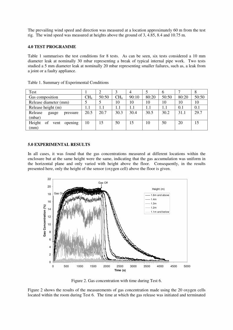
Figure 2. Gas concentration with time during Test 6.
Figure 2 shows the results of the measurements of gas concentration made using the 20 oxygen cells
located within the room during Test 6. The time at which the gas release was initiated and terminated
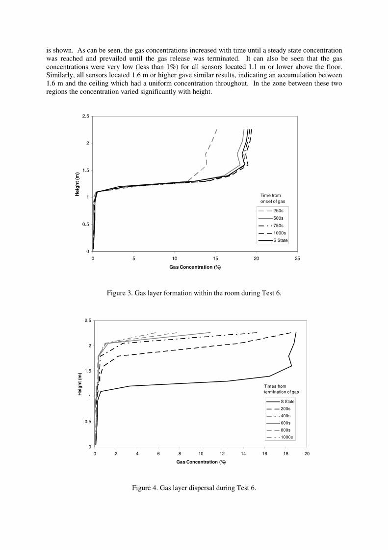
is shown. As can be seen, the gas concentrations increased with time until a steady state concentration
was reached and prevailed until the gas release was terminated. It can also be seen that the gas
concentrations were very low (less than 1%) for all sensors located 1.1 m or lower above the floor.
Similarly, all sensors located 1.6 m or higher gave similar results, indicating an accumulation between
1.6 m and the ceiling which had a uniform concentration throughout. In the zone between these two
regions the concentration varied significantly with height.
0
0.5
1
1.5
2
2.5
0 5 10 15 20 25
Gas Concentration (%)
Heig
ht
(m)
250s
500s
750s
1000s
S State
Time from
onset of gas
Figure 3. Gas layer formation within the room during Test 6.
0
0.5
1
1.5
2
2.5
0 2 4 6 8 10 12 14 16 18 20
Gas Concentration (%)
Heig
ht
(m)
S State
200s
400s
600s
800s
1000s
Times from
termination of gas
Figure 4. Gas layer dispersal during Test 6.
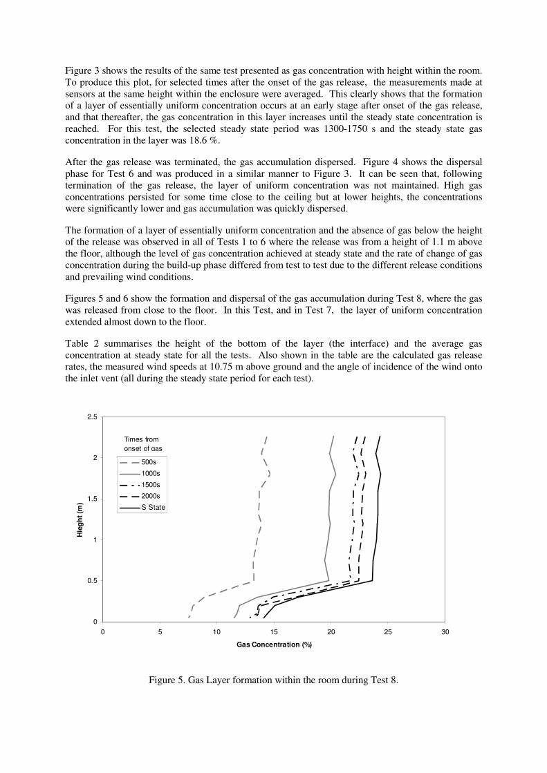
Figure 3 shows the results of the same test presented as gas concentration with height within the room.
To produce this plot, for selected times after the onset of the gas release, the measurements made at
sensors at the same height within the enclosure were averaged. This clearly shows that the formation
of a layer of essentially uniform concentration occurs at an early stage after onset of the gas release,
and that thereafter, the gas concentration in this layer increases until the steady state concentration is
reached. For this test, the selected steady state period was 1300-1750 s and the steady state gas
concentration in the layer was 18.6 %.
After the gas release was terminated, the gas accumulation dispersed. Figure 4 shows the dispersal
phase for Test 6 and was produced in a similar manner to Figure 3. It can be seen that, following
termination of the gas release, the layer of uniform concentration was not maintained. High gas
concentrations persisted for some time close to the ceiling but at lower heights, the concentrations
were significantly lower and gas accumulation was quickly dispersed.
The formation of a layer of essentially uniform concentration and the absence of gas below the height
of the release was observed in all of Tests 1 to 6 where the release was from a height of 1.1 m above
the floor, although the level of gas concentration achieved at steady state and the rate of change of gas
concentration during the build-up phase differed from test to test due to the different release conditions
and prevailing wind conditions.
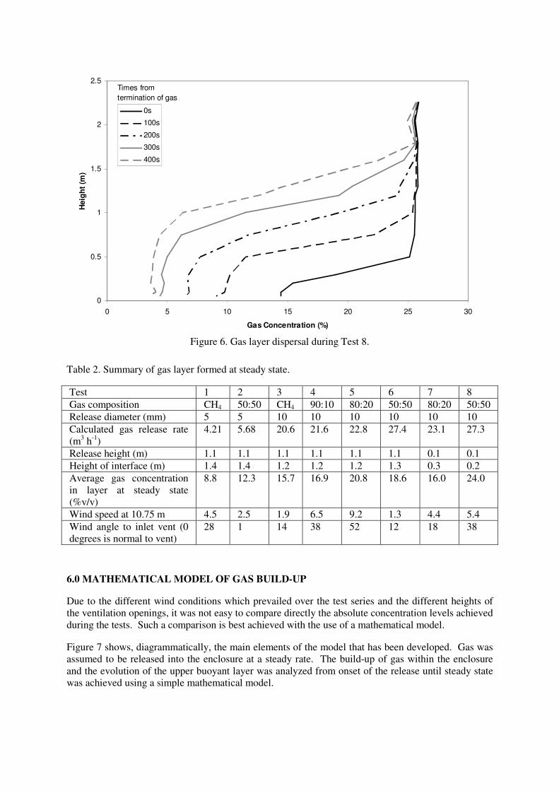
Figures 5 and 6 show the formation and dispersal of the gas accumulation during Test 8, where the gas
was released from close to the floor. In this Test, and in Test 7, the layer of uniform concentration
extended almost down to the floor.
Table 2 summarises the height of the bottom of the layer (the interface) and the average gas
concentration at steady state for all the tests. Also shown in the table are the calculated gas release
rates, the measured wind speeds at 10.75 m above ground and the angle of incidence of the wind onto
the inlet vent (all during the steady state period for each test).
0
0.5
1
1.5
2
2.5
0 5 10 15 20 25 30
Gas Concentration (%)
Hie
gh
t (m
)
500s
1000s
1500s
2000s
S State
Times from
onset of gas
Figure 5. Gas Layer formation within the room during Test 8.
0
0.5
1
1.5
2
2.5
0 5 10 15 20 25 30
Gas Concentration (%)
Heig
ht
(m)
0s
100s
200s
300s
400s
Times from
termination of gas
Figure 6. Gas layer dispersal during Test 8.
Table 2. Summary of gas layer formed at steady state.
Test 1 2 3 4 5 6 7 8
Gas composition CH4 50:50 CH4 90:10 80:20 50:50 80:20 50:50
Release diameter (mm) 5 5 10 10 10 10 10 10
Calculated gas release rate
(m3 h
-1)
4.21 5.68 20.6 21.6 22.8 27.4 23.1 27.3
Release height (m) 1.1 1.1 1.1 1.1 1.1 1.1 0.1 0.1
Height of interface (m) 1.4 1.4 1.2 1.2 1.2 1.3 0.3 0.2
Average gas concentration
in layer at steady state
(%v/v)
8.8 12.3 15.7 16.9 20.8 18.6 16.0 24.0
Wind speed at 10.75 m 4.5 2.5 1.9 6.5 9.2 1.3 4.4 5.4
Wind angle to inlet vent (0
degrees is normal to vent)
28 1 14 38 52 12 18 38
6.0 MATHEMATICAL MODEL OF GAS BUILD-UP
Due to the different wind conditions which prevailed over the test series and the different heights of
the ventilation openings, it was not easy to compare directly the absolute concentration levels achieved
during the tests. Such a comparison is best achieved with the use of a mathematical model.
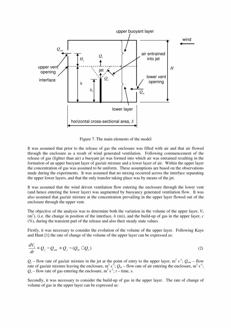
Figure 7 shows, diagrammatically, the main elements of the model that has been developed. Gas was
assumed to be released into the enclosure at a steady rate. The build-up of gas within the enclosure
and the evolution of the upper buoyant layer was analyzed from onset of the release until steady state
was achieved using a simple mathematical model.
inQ
pQ
outQ
1H
sQ
hs h
lower vent opening interface
H
upper buoyant layer
lower layer
upper vent opening
air entrained into jet
jet
wind
horizontal cross-sectional area, S
Qj
Figure 7. The main elements of the model
It was assumed that prior to the release of gas the enclosure was filled with air and that air flowed
through the enclosure as a result of wind generated ventilation. Following commencement of the
release of gas (lighter than air) a buoyant jet was formed into which air was entrained resulting in the
formation of an upper buoyant layer of gas/air mixture and a lower layer of air. Within the upper layer
the concentration of gas was assumed to be uniform. These assumptions are based on the observations
made during the experiments. It was assumed that no mixing occurred across the interface separating
the upper lower layers, and that the only transfer taking place was by means of the jet.
It was assumed that the wind driven ventilation flow entering the enclosure through the lower vent
(and hence entering the lower layer) was augmented by buoyancy generated ventilation flow. It was
also assumed that gas/air mixture at the concentration prevailing in the upper layer flowed out of the
enclosure through the upper vent.
The objective of the analysis was to determine both the variation in the volume of the upper layer, V1
(m3), (i.e. the change in position of the interface, h (m)), and the build-up of gas in the upper layer, c
(%), during the transient part of the release and also their steady state values.
Firstly, it was necessary to consider the evolution of the volume of the upper layer. Following Kaye
and Hunt [1] the rate of change of the volume of the upper layer can be expressed as:
)(1sinjoutj QQQQQ
dt
dV+−=−= (2)
Qj – flow rate of gas/air mixture in the jet at the point of entry to the upper layer, m3 s
-1; Qout – flow
rate of gas/air mixture leaving the enclosure, m3 s
-1; Qin – flow rate of air entering the enclosure, m
3 s
-1;
Qs – flow rate of gas entering the enclosure, m3 s
-1; t – time, s.
Secondly, it was necessary to consider the build-up of gas in the upper layer. The rate of change of
volume of gas in the upper layer can be expressed as:
( ))(1
11
sins QQcQdt
dVc
dt
dcV
dt
cVd+−=+= (3)
Substituting for dt
dV1 from equation (2), gives:
( )( ) )(1 sinssinj QQcQQQQcdt
dcV +−=+−+
Therefore the rate of change of the concentration is given by:
js cQQdt
dcV −=1 (4)
To solve the pair of equations (2) and (4) numerically, it was necessary to establish relationships for
the volume flow rate of ventilation air into the enclosure through the lower vent, Qin, and the volume
flow rate of gas/air mixture from the jet into the upper layer, Qj.
To determine Qin, the approach described in Warren and Webb (1980) [2] was followed in which:
22
WBin QQQ += (5)
QB - ventilation flow generated by buoyancy in the absence of wind, m3 s
-1; QW - ventilation flow
generated by the wind in the absence of buoyancy, m3s
-1.
Considering the effective height of the upper buoyant layer as the vertical distance from the interface
to the centre of the upper vent, H1, (m) then the ventilation flow generated by buoyancy can be
expressed as:
122
HgAC
Q vdB
′= (6)
Cd – coefficient of discharge of the vent (A value of Cd = 0.8 was used.) ; Av – area of vent opening,
m2; g′ - reduced gravity, m s
-2.
Where ggair
air
−=′
ρρρ 1
g – acceleration due to gravity, m s-2
; ρair – density of air, kg m-3
; ρ1 – density of gas/air mixture in the
upper layer, kg m-3
.
The ventilation flow generated by the wind can be expressed as:
Wvd
W UAC
Q2
= (7)
UW – component of the wind velocity normal to the ventilation opening, m s-1
.
To determine Qj, the model for a buoyant jet of Lane-Serff et al (1993) [3] was adopted. The two
main assumptions of this approach are the Boussinesq approximation (discussed in detail by Turner
(1973) [4]) and relating entrainment into the jet as proportional to the local mean jet velocity. The
constant of proportionality is called the entrainment constant, α.
An entrainment constant was first used explicitly by Morton, Taylor and Turner (1956) [5]. Numerous
experimental studies have provided values of the entrainment constant such as Rouse, Yih and
Humphreys (1952) [6], Chen and Rodi (1980) [7]. A value of α = 0.05 taken from Rodi (1982) [8] was
used in this analysis.
Following Lane-Serff et al (1993) [3], Conservation equations for mass, momentum and buoyancy
were written as:
( )j
jUR
dZ
RUdα2
2
= (8a)
( ) ( )2
22
RgdZ
RUd j λ′= (8b)
( )0
2
=′dZ
RUgd j (8c)
Uj – local mean jet velocity, m s-1
; R – local jet radius, m; Z – height above the source of the gas, m; λ
– ratio of the transverse length scales of density and velocity. (Following Lane-Serff et al (1993) [3], a
value of λ of 1.1 was adopted.)
Equations (8a) to (8c) were non-dimensionalised and transformed as described by Lane-Serff et al
(1993) [3] and integrated at each time step during the solution of equations (2) and (4) to determine the
mean jet velocity, Uj, and the jet radius, R, at the height at which the jet entered the upper buoyant
layer. This enabled the flow rate of gas/air mixture into the upper layer, Qj, to be calculated.
7.0 RESULTS FROM THE MODEL
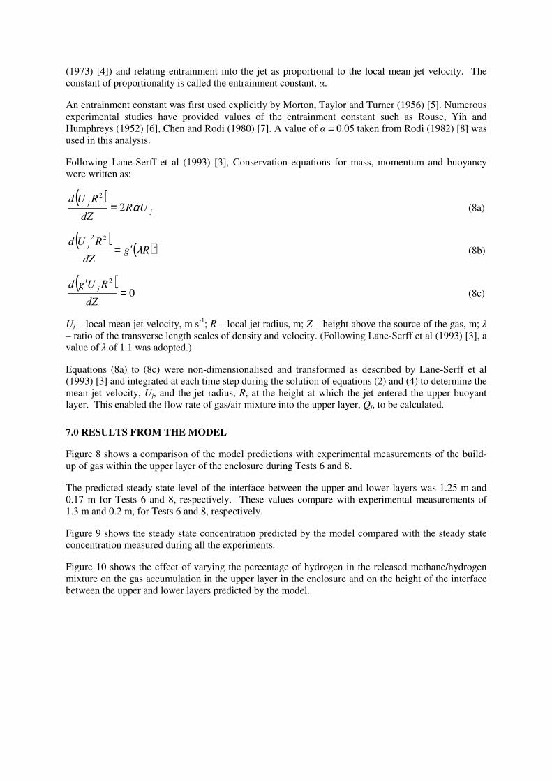
Figure 8 shows a comparison of the model predictions with experimental measurements of the build-
up of gas within the upper layer of the enclosure during Tests 6 and 8.
The predicted steady state level of the interface between the upper and lower layers was 1.25 m and
0.17 m for Tests 6 and 8, respectively. These values compare with experimental measurements of
1.3 m and 0.2 m, for Tests 6 and 8, respectively.
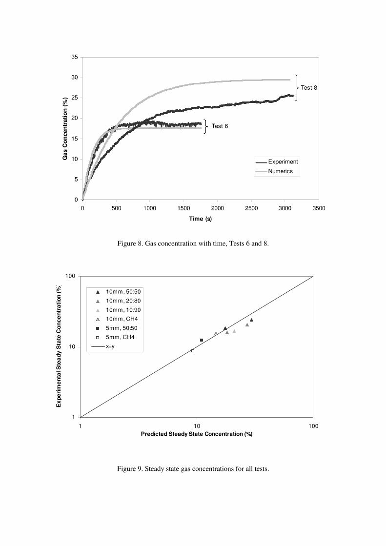
Figure 9 shows the steady state concentration predicted by the model compared with the steady state
concentration measured during all the experiments.
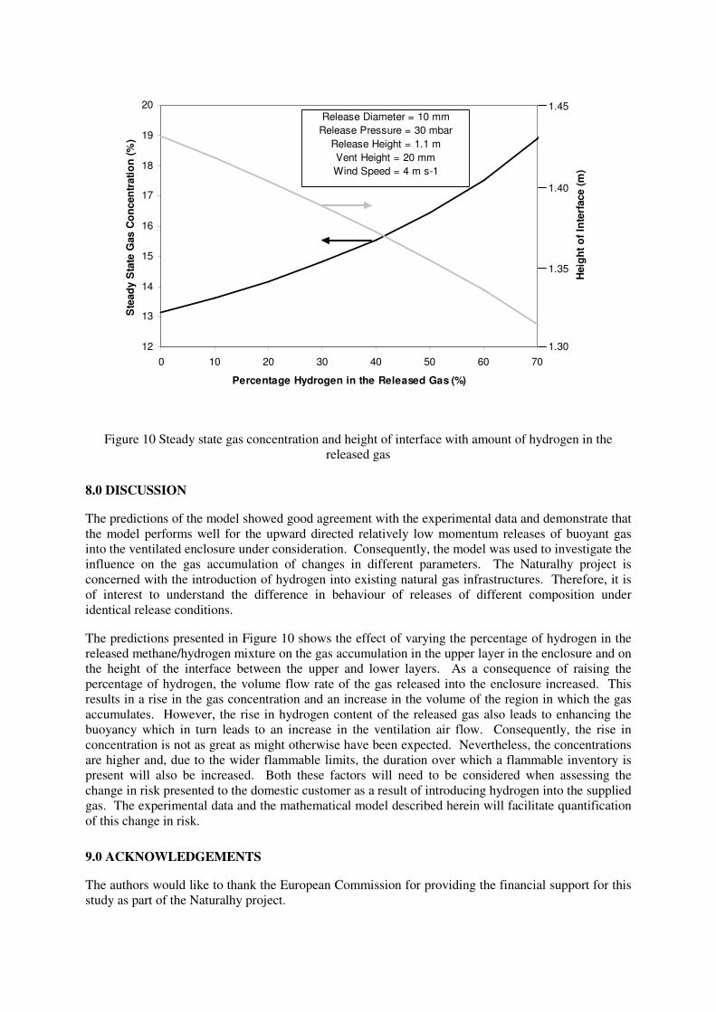
Figure 10 shows the effect of varying the percentage of hydrogen in the released methane/hydrogen
mixture on the gas accumulation in the upper layer in the enclosure and on the height of the interface
between the upper and lower layers predicted by the model.
0
5
10
15
20
25
30
35
0 500 1000 1500 2000 2500 3000 3500
Time (s)
Gas C
on
cen
trati
on
(%
)
Experiment
Numerics
Test 6
Test 8
Figure 8. Gas concentration with time, Tests 6 and 8.
1
10
100
1 10 100
Predicted Steady State Concentration (%)
Ex
pe
rim
en
tal S
tea
dy
Sta
te C
on
ce
ntr
ati
on
(%
)
10mm, 50:50
10mm, 20:80
10mm, 10:90
10mm, CH4
5mm, 50:50
5mm, CH4
x=y
Figure 9. Steady state gas concentrations for all tests.
12
13
14
15
16
17
18
19
20
0 10 20 30 40 50 60 70
Percentage Hydrogen in the Released Gas (%)
Ste
ad
y S
tate
Gas C
on
cen
trati
on
(%
)
Release Diameter = 10 mm
Release Pressure = 30 mbar
Release Height = 1.1 m
Vent Height = 20 mm
Wind Speed = 4 m s-1
1.45
1.40
1.35
1.30
Heig
ht
of
Inte
rface (
m)
Figure 10 Steady state gas concentration and height of interface with amount of hydrogen in the
released gas
8.0 DISCUSSION
The predictions of the model showed good agreement with the experimental data and demonstrate that
the model performs well for the upward directed relatively low momentum releases of buoyant gas
into the ventilated enclosure under consideration. Consequently, the model was used to investigate the
influence on the gas accumulation of changes in different parameters. The Naturalhy project is
concerned with the introduction of hydrogen into existing natural gas infrastructures. Therefore, it is
of interest to understand the difference in behaviour of releases of different composition under
identical release conditions.
The predictions presented in Figure 10 shows the effect of varying the percentage of hydrogen in the
released methane/hydrogen mixture on the gas accumulation in the upper layer in the enclosure and on
the height of the interface between the upper and lower layers. As a consequence of raising the
percentage of hydrogen, the volume flow rate of the gas released into the enclosure increased. This
results in a rise in the gas concentration and an increase in the volume of the region in which the gas
accumulates. However, the rise in hydrogen content of the released gas also leads to enhancing the
buoyancy which in turn leads to an increase in the ventilation air flow. Consequently, the rise in
concentration is not as great as might otherwise have been expected. Nevertheless, the concentrations
are higher and, due to the wider flammable limits, the duration over which a flammable inventory is
present will also be increased. Both these factors will need to be considered when assessing the
change in risk presented to the domestic customer as a result of introducing hydrogen into the supplied
gas. The experimental data and the mathematical model described herein will facilitate quantification
of this change in risk.
9.0 ACKNOWLEDGEMENTS
The authors would like to thank the European Commission for providing the financial support for this
study as part of the Naturalhy project.

10.0 REFERENCES
1. Kaye, N.B. and Hunt, G.R., Time-dependent flows in an emptying filling box, J. Fluid Mech. 520,
2004, pp. 135-156.
2. Warren, P.R. and Webb, B.C. The relationship between tracer gas and pressurisation techniques in
dwellings. Proc. 1st AIC Conf. “Instrumentation and Measurement Techniques”, Windsor, UK,
1980, pp. 245-276.
3. Lane-Serff, G.F., Linden, P.F. and Hillel, M., Forced, angled plumes, Journal of Hazardous
Materials, 33, 1993, pp. 75-99.
4. Turner,J.S. Buoyancy effects in fluids. Cambridge University Press, London, 1973.
5. Morton, B.R., Taylor,G.I. and Turner,J.S. Turbulent gravitational convection from maintained and
instantaneous sources. Proc. R. Soc. London A 234, 1956, pp. 1-23.
6. Rouse, H., Yih, C.S. and Humphreys, H.W., Gravitational convection from a boundary source,
Tellus, 4, 1952, pp. 201-210.
7. Chen, C.J. and Rodi, W. Vertical turbulent buoyant jets: A review of experimental data, Pergamon
Press, Oxford, 1980
8. Rodi, W. Turbulent Buoyant Jets and Plumes, Pergamon Press, Oxford, 1982, pp. 47.


![How To Build Your Own Domestic Violence Case Without A Lawyer [v1]](https://img.pdfslide.us/doc/110x75/55cf8e10550346703b8e202e/how-to-build-your-own-domestic-violence-case-without-a-lawyer-v1.jpg)