GARCH Option Pricing Models, the CBOE VIX, and Variance ... · PDF filepapers discussing the weakness of traditional GARCH option pricing models. Garcia and Renault ... for both the

[11:29 14/6/2013 nbs026.tex] JFINEC: Journal of Financial Econometrics Page: 556 556–580

Journal of Financial Econometrics, 2013, Vol. 11, No. 3, 556--580

GARCH Option Pricing Models, the CBOEVIX, and Variance Risk PremiumJINJI HAO

Department of Economics, Washington University in St. Louis

JIN E. ZHANG

Department of Accountancy and Finance, Otago Business School,University of Otago and School of Economics and Finance, The Universityof Hong Kong

ABSTRACTIn this article, we derive the corresponding implied VIX formulas underthe locally risk-neutral valuation relationship (LRNVR) proposed byDuan (1995) when a class of square-root stochastic autoregressivevolatility (SR-SARV) models are proposed for S&P 500 index. Theempirical study shows that the GARCH implied VIX is consistently andsignificantly lower than the CBOE VIX for all kinds of GARCH modelinvestigated when they are estimated with returns only. When jointlyestimated with both returns and VIX, the parameters are distortedunreasonably, and the GARCH implied VIX still cannot fit the CBOEVIX from various statistical aspects. The source of this discrepancyis then theoretically analyzed. We conclude that the GARCH optionpricing under the LRNVR fails to incorporate the price of volatility orvariance risk premium. ( JEL: G13, C52)

KEYWORDS: GARCH option pricing models, GARCH implied VIX, the CBOEVIX, Variance risk premium

We are especially grateful to Eric Renault (editor) and two anonymous referees whose helpful commentssubstantially improved the paper. We also acknowledge helpful comments from Andrew Carverhill(our AsianFA discussant), Werner Ploberger, Jinghong Shu, Tianyi Wang, Dongming Zhu and seminarparticipants at Peking University, Asian Finance Association (AsianFA) 2010 International Conference inHong Kong. Jin E. Zhang has been supported by a grant from the Research Grants Council of the HongKong Special Administrative Region, China (Project No. HKU 7549/09H). Address correspondence to JinE. Zhang, School of Economics and Finance, The University of Hong Kong, Pokfulam Road, Hong Kong,P. R. China, or e-mail: [email protected]

doi:10.1093/jjfinec/nbs026 Advanced Access publication January 20, 2013© The Author, 2013. Published by Oxford University Press. All rights reserved.For Permissions, please email: [email protected]


HAO & ZHANG | GARCH Option Pricing Models 557

1 INTRODUCTION

Finance literature has put much effort on studying the premia that investorsrequire for compensating various risks in financial market, especially the equityrisk premium for price risk (volatility). However, instead of a constant volatilityassumed in the Black–Scholes framework, a lot of research has confirmed that thevolatility itself is time-varying, which is termed volatility risk. Many stochasticvolatility models and various GARCH models go along this line.

Then a natural question is whether this volatility risk is priced and compen-sated in financial market. One of the possible rationales for the existence of volatilityrisk premium is the negative correlation between the volatility and the index, whichhas been verified in many literatures. In the context of asset pricing theory, thesource of risk is the correlation with the market portfolio, aggregate consumption orpricing kernel. Theoretically, the negative correlation between volatility and indexsuggests a negative risk premium. If so, the premia required by investors should bereflected in the prices of volatility-dependent assets such as options and volatilityproducts. The pursuit of empirical evidence generally proceeds in two directions.One is to study the phenomenon that the implied volatility of options exceeds therealized volatility. Various delta-neutral portfolios of options are constructed to testwhether significant gains or losses could be produced. Another one is to investigatethe difference between the variance swap rate and the realized variance, which iscoined variance premium. Variance swap rate, the risk-neutral expectation of thefuture variance, can be replicated with European options (See Demeterfi et al., 1999;Carr and Wu, 2009). Methodologies for calculating a model-free realized variancehave also been developed (see Andersen et al., 2003).

Since 1980s, option pricing models with stochastic volatility have introducedthe market price of volatility risk when changing from the physical probabilitymeasure to the risk-neutral measure. These papers include Wiggins (1987),Johnson and Shanno (1987), Hull and White (1987), Scott (1987) and Heston (1993).However, they set the market price of volatility risk to either zero or a constant anddiscussed little about the size, sign or dynamics of this parameter.

Since the beginning of this century, the evidence of the existence of volatilityrisk premium has been well documented. Coval and Shumway (2001) studiedthe expected option return under the framework of classic asset pricing theory.They showed that the zero-beta, at the money straddles that are in longpositions of volatility suffer from average weekly losses of about three percent.Bakshi and Kapadia (2003) constructed a correspondence between the sign andmagnitude of volatility risk premium and the mean delta-hedged portfolio returns.Their empirical results indicated a negative market volatility risk premium.Carr and Wu (2009) calculated the variance premia for several stock market indexesthrough replications with options, and average negative variance premium wasshown.

The dynamics and driving forces of variance premium are studied in recent lit-erature. Vilkov (2008) used the synthetic variance swap returns to approximate the


558 Journal of Financial Econometrics

variance risk premium and studied the dynamics and cross-sectional properties ofvariance premia embedded in index options and individual stock options. Todorov(2010) studied variance risk in terms of stochastic volatility and jumps. Model-free realized variance and realized jumps are constructed using high-frequencydata. He found that price jumps play an important role in explaining the variancerisk premium. Specifically, the estimated variance risk premium increases after abig market jump and slowly reverts to its long-run mean thereafter. Eraker (2008)captured the volatility premium and the large negative correlation between shocksto volatility and stock price with a general equilibrium based on long-run risk.

In this article, we investigate whether the GARCH option pricing model cancapture the variance premium. Since the seminal autoregressive conditional het-eroscedasticity (ARCH) model of Engle (1982) and the generalized autoregressiveconditional heteroscedasticity (GARCH) model of Bollerslev (1986), the GARCHmodels have attracted huge attention from the academics and practitioners andhave been intensively used to model the financial times series. This is mostlybecause they can capture the volatility clustering and fat tails that are typicalproperties of the financial time series. The family of GARCH models has alsobeen enriched to capture the stylized fact that negative returns have higher impacton the volatility than positive ones, which is called leverage effect. This class ofGARCH models includes the exponential GARCH (EGARCH) of Nelson (1991),the threshold GARCH (TGARCH) of Glosten, Jagannathan, and Runkle (1993) andthe non-linear asymmetric GARCH (AGARCH) of Engle and Ng (1993) and the like.Engle and Lee (1993) introduced the component GARCH (CGARCH) that separatesthe conditional variance into a transitory component and a permanent component.

Duan (1995) pioneered in employing the GARCH model in the optionpricing theory. He put forward an equilibrium argument that the options canbe priced under a locally risk-neutral valuation relationship (LRNVR) with someassumptions on the utility function when the price of the underlying asset followsa GARCH process. Kallsen and Taqqu (1998) considered a broad class of ARCH-type models embedded into a continuous-time framework and derived the sameresult by a no-arbitrage argument. The GARCH option pricing model has somelinkage with those bivariate diffusion option pricing models. Duan (1996, 1997),showed that most variants of GARCH model mentioned above converge to thebivariate diffusion processes commonly used for modeling the stochastic volatility.Ritchken and Trevor (1999) developed a lattice algorithm that is applicable foroption pricing under both GARCH models and bivariate diffusions. We will furtherdiscuss this limiting property in this article.

The concept of LRNVR in Duan (1995) has been mainly followed by thesubsequent GARCH option pricing literature, for instance, Heston and Nandi(2000), Christoffersen and Jacobs (2004) and Christoffersen et al. (2008) amongthe others.1 Garcia, Ghysels, and Renault (2010) provided an interesting and

1In this article, we focus on Gaussian GARCH option pricing models with LRNVR. For theGARCH models with non-Gaussian innovations, the literature on changing probability measures



comprehensive review on the econometrics of option pricing models. We willalso focus on Duan’s option pricing model in this article. There are severalpapers discussing the weakness of traditional GARCH option pricing models.Garcia and Renault (1998) pointed out that the hedging formula given in Duan(1995) is not consistent with the fact that the GARCH option pricing is nothomogeneous of degree one with respect to the spot price and the strike price. Anew GARCH option pricing model with filtered historical simulation developed byBarone-Adesi, Engle, and Mancini (2008) avoided a change of probability measureby directly calibrating a new risk neutral GARCH model on option prices. The mostrelevant research to our work is Christoffersen, Heston, and Jacobs (2011) in whichthey propose a variance-dependent pricing kernel for GARCH model accountingfor both the equity risk premium and the variance risk premium.2

To study the variance premium captured by GARCH option pricing models, wewill derive the GARCH implied VIX3 under the LRNVR proposed by Duan (1995).To do this, a more general class of square-root stochastic autoregressive volatility(SR-SARV) models (Meddahi and Renault, 2004) which subsumes many specificGARCH models is proposed for the S&P 500 index. We calculate the (squared)VIX as a risk-neutral expectation of the average variance over the next 21 tradingdays under the LRNVR. In this article, GARCH(1,1) and four other variants ofGARCH(1,1) model are numerically estimated with different data sets.

We then compare the GARCH implied VIX with the CBOE VIX. We find thatthe GARCH implied VIX is significantly and consistently lower than the CBOEVIX when only returns are used for estimation. The difference is around 3.6 thatis consistent with the empirical evidence of the size of volatility premium. WhenVIX is used for estimation, the parameters, especially the equity risk premium,

from physical to risk-neutral ones is still under development. For example, Duan (1999) uses Box-Cox transformation to introduce conditional fat-tailed innovations; Siu, Tong, and Yang (2004) relyon the conditional Esscher transformation to incorporate infinitely divisible distributed innovation;Christoffersen, Heston, and Jacobs (2006) develop a model with Inverse Gaussian innovation allowingfor conditional skewness; Christoffersen et al. (2010) characterize the Radon-Nikodym derivative forneutralizing a class of GARCH models with more general innovations. It is an interesting researchtopic to examine the performance of these non-Gaussian GARCH option pricing models in capturingthe variance risk premium. However, under normality, Duan (1999) and Siu, Tong, and Yang (2004) givethe same result as Duan (1995) with LRNVR, and Christoffersen et al. (2010) subsumes Duan (1995) andHeston and Nandi (2000) as special cases. It would be reasonable to suspect that these models might havesimilar problem observed in this article. Certain amount of research needs to be done in order to makeany conclusion. We decide to leave this topic for the future research.

2We share the same view that ‘The filtering problem in these models [GARCH dynamics] is straightforwardbecause the distribution of one-period return has a known conditional variance .... it has implication foroption pricing. Because the models do not contain an independent adjustment for variance risk, they donot offer much flexibility in the modeling of variance risk premia’ (Christoffersen, Heston, and Jacobs,2011).

3VIX is the Chicago Board of Exchange (CBOE) listed volatility index, which is updated in 2004 and reflectsexpectations of the volatility of the S&P 500 index over the next 30 calendar days. Demeterfi et al. (1999)showed that the squared VIX is actually the variance swap rate and can be replicated with a portfolio ofoptions written on the S&P 500 index.



are distorted to unreasonable levels, and the statistics of the CBOE VIX remainunmatched.

The source of this discrepancy is then theoretically analyzed. We investigatethe LRNVR and the diffusion limits of the GARCH model under both the physicalmeasure and the LRNVR. It is shown that the innovation of volatility is invariantwith respect to the change of probability measure with the LRNVR, and nopremium for the volatility risk is compensated.

The article is constructed as follows. In Section 2, we first review the LRNVR ofDuan (1995) for changing probability measure for the GARCH(p,q) model. We thenderive VIX formulas under the LRNVR for a broad class of GARCH models and itsextension, which subsume GARCH, TGARCH, AGARCH, CGARCH, and EGARCHmodels. In Section 3, we estimate these models using time series of the S&P 500index and the CBOE VIX. The GARCH implied VIX is computed and comparedwith the CBOE VIX in Section 4. In Section 5, the failure of the GARCH optionpricing under the LRNVR to incorporate the price of volatility risk is analyzed. Weconclude in Section 6.

2 THEORETICAL RESULTS ON GARCH IMPLIED VIX

2.1 GARCH Option Pricing Models

Duan (1995) utilized a linear GARCH process for modeling the underlying assetand pricing the options written on it. In that article, the return of the asset in eachperiod is modeled to follow a conditional lognormal distribution under the physicalmeasure P,

lnXt

Xt−1=r+λ

√ht − 1

2ht +εt, (1)

where Xt is the price of the asset, r is the constant interest rate, and λ is the riskpremium; εt follows a GARCH(p,q) process

εt |φt−1 ∼N(0,ht) under measure P,

ht =α0 +q∑

i=1

αiε2t−i +

p∑i=1

βiht−i, (2)

where φt is the information set of all information up to and including time t; p≥0,q≥0; α0>0, αi ≥0, i=1, ··· ,q; βi ≥0, i=1, ··· ,p.

With assumptions made on the utility function and the aggregated consump-tion growth, Duan (1995) proposed a new locally risk neutral valuation relationship,Q, under which

lnXt

Xt−1=r− 1

2ht +ξt, (3)



and

ξt |φt−1 ∼N(0,ht),

ht =α0 +q∑

i=1

αi

(ξt−i −λ

√ht−i

)2 +p∑

i=1

βiht−i. (4)

2.2 GARCH Implied VIX

VIX reflects investors’ expectation of the volatility of the S&P 500 index in thefollowing 30 calender days, that is(

VIXt

100

)2=EQ

t

[1τ0

∫ t+τ0

thsds

], (5)

where τ0 =30 calendar days or 21 trading days, and hs is the instantaneousannualized variance of the rate of return of S&P 500. In this article, we calculateVIX as an expected arithmetic average of the variance in the n subperiods of thefollowing 30 calendar days, that is(

VIXt

100

)2= 1

n

n∑k=1

EQt

[h

t+ τ0kn

]. (6)

Especially, we will use data with daily frequency, that is τ0 =n, then

Vixt = 1n

n∑k=1

EQt [ht+k], (7)

where Vixt = 1252 ( VIXt

100 )2 is defined as a proxy for VIXt in terms of daily variance.The conditional mean of future variance can be calculated under a broad class

of GARCH models. We will consider the square-root stochastic autoregressivevolatility (SR-SARV) models (Meddahi and Renault, 2004).

Definition 1: (Discrete time SR-SARV(p) model, Meddahi and Renault, 2004). Astationary square-integrable process {εt,t∈Z} is called a SR-SARV(p) process with respectto a filtration Jt,t∈Z, if:

(i) εt is a martingale difference sequence (m.d.s.) w.r.t. Jt−1, that is E[εt|Jt−1]=0,(ii) the conditional variance process ft of εt+1

4 given Jt is a marginalization of a stationaryJt-adapted VAR(1) of dimension p:

ft ≡Var[εt+1|Jt]=e′Ft, (8)

Ft =+�Ft−1 +Vt, with E[Vt|Jt−1]=0, (9)

4Indeed, ft =ht+1. But we adopt the notations in Meddahi and Renault (2004) here.



where e∈Rp,∈R

p and the eigenvalues of � have modulus less than one.

If the S&P 500 follows a SR-SARV(p) process under the risk neutral measure, ananalytical formula for the GARCH implied VIX can be obtained.

Proposition 1: If the S&P 500 follows a SR-SARV(p) process under the locally riskneutral valuation relationship Q proposed by Duan (1995), then the implied VIX at time tis affine in Ft, i.e.,

Vixt =ζ+ Ft, ∈Rp. (10)

In particular, if p=1 (then e=1), the implied VIX at time t is a linear function of theconditional variance of the next period,

Vixt =ζ+ψ ft, ψ ∈R, (11)

where

ζ =

1−� (1−ψ),

ψ= 1−�n

n(1−�).

Proof. See Appendix. �

In particular, the threshold GARCH(1,1) (TGARCH) ofGlosten, Jagannathan, and Runkle (1993), the non-linear asymmetric GARCH(1,1)(AGARCH) of Engle and Ng (1993) and the component GARCH(1,1) (CGARCH)of Engle and Lee (1993), which are widely used, are special cases of SR-SARV(p)models. In specific, they take the forms of the following:

TGARCH(1,1):

Physical measure :ht =α0 +α1ε2t−1 +θε2

t−11(εt−1<0)+β1ht−1, (12)

LRNVR :ht =α0 +(ξt−1 −λ√ht−1

)2[α1 +θ1

(ξt−1 −λ√ht−1<0

)]+β1ht−1. (13)

AGARCH(1,1):

Physical measure :ht =α0 +α1

(εt−1 −θ√ht−1

)2 +β1ht−1, (14)

LRNVR :ht =α0 +α1

(ξt−1 −λ√ht−1 −θ√ht−1

)2 +β1ht−1. (15)

CGARCH(1,1):

Physical measure:

ht −qt =α1

(ε2

t−1 −qt−1

)+β1

(ht−1 −qt−1

), (16)



qt =α0 +ρqt−1 +φ(ε2

t−1 −ht−1

).

LRNVR:

ht −qt =α1

[(ξt−1 −λ√ht−1

)2 −qt−1

]+β1

(ht−1 −qt−1

), (17)

qt =α0 +ρqt−1 +φ[(ξt−1 −λ√ht−1

)2 −ht−1

].

Proposition 2: Let {ξt,t∈Z} be a m.d.s. with the conditional variance ht ≡Var[ξt|ξτ ,τ ≤t−1] under the LRNVR. If ht is given by (4) or (15), then ξt is a SR-SARV(1) process. Ifht is given by (17) , then ξt is a SR-SARV(2) process. Furthermore, if ut =ξt/

√ht is i.i.d.,

the TGARCH model (13) is also a SR-SARV(1) process.5

Proof. See Appendix. �

In this article, we assume εt/√

ht and ξt/√

ht are i.i.d. under the physical mea-sure and the LRNVR, respectively, which is sufficient for this proposition to be true.

Corollary 1: Under the locally risk neutral valuation relationship Q proposed by Duan(1995), if the S&P 500 follows a GARCH(1,1), TGARCH(1,1) or AGARCH(1,1) process,the implied VIX is a linear function of the conditional variance of the next period, ht+1. Ifthe S&P 500 follows a CGARCH(1,1) process, the implied VIX is a linear function of thetransitory and permanent components of the conditional variance of the next period, ht+1and qt+1.

The specific VIX formulas are given in Appendix.Now we extend the SR-SARV model to a square-root stochastic exponential

autoregressive volatility (SR-SEARV) model:

Definition 2: (Discrete time SR-SEARV(1) model). A stationary square-integrableprocess {εt,t∈Z} is called a SR-SEARV(1) process with respect to a filtration Jt,t∈Z,if:

(i) εt is a martingale difference sequence w.r.t. Jt−1, that is E[εt|Jt−1]=0,(ii) the logarithm of the conditional variance process ft of εt+1 given Jt is a stationary

Jt-adapted AR(1):

ln ft =ω+γ ln ft−1 +vt, with vt i.i.d. (18)

where |γ |<1.

5Under the LRNVR, the VGARCH model discussed in Meddahi and Renault (2004) is also a SR-SARV(1),while the Asymmetric GARCH model, a different version used in Meddahi and Renault (2004), and theHeston and Nandi model are not because

√ht terms would appear in the expressions of conditional

variance after the risk neutralization.



Proposition 3: If the S&P 500 follows a SR-SEARV(1) process under the locally riskneutral valuation relationship Q proposed by Duan (1995), then the implied VIX is apolynomial function of the conditional variance of the next period, ht+1.

We will show that the EGARCH(1,1) model is a SR-SEARV(1) below.

EGARCH(1,1):

Physical measure :ln ht =α0 +β1 ln ht−1 +g(zt−1), zt =εt/

√ht, (19)

g(zt−1)=α1zt−1 +κ(|zt−1|−

√2/π

).

LRNVR :ln ht =α0 +β1 ln ht−1 +g(ut−1 −λ), ut =ξt/

√ht, (20)

g(ut−1 −λ)=α1(ut−1 −λ)+κ(|ut−1 −λ|−√

2/π).

Proposition 4: If {ξt,t∈Z} is a m.d.s. under the LRNVR with the conditional varianceht ≡Var[ξt|ξτ ,τ ≤ t−1] given by (20) and ut =ξt/

√ht i.i.d., then ξt is a SR-SEARV(1)

process.

Let vt =g(ut −λ). Since ut is i.i.d., vt is also i.i.d., and the EGARCH(1,1) model is aSR-SEARV(1).

Corollary 2: If the S&P 500 follows an EGARCH(1,1) process under the locally riskneutral valuation relationship Q proposed by Duan (1995), the implied VIX is a polynomialfunction of the conditional variance of the next period, ht+1.

The specific VIX formula is also given in Appendix.

3 DATA AND ESTIMATION

Based on the theoretical results obtained in last section, a natural question iswhether the GARCH implied VIX fits the market VIX well. In this section, wewill investigate it by estimating GARCH models and calculating correspondingVIX times series.

In this article, we will use two time series data from the closing price of S&P 500index and the CBOE VIX ranging from January 2, 1990 to August 10, 2009. We alsouse the daily 3-month U.S. Treasury bills (secondary market) rate as the risk-freerate and we get this time series data from the Federal Reserve website.



We may have different approaches in estimating the models. The firststraightforward one is to run a maximum likelihood estimation of the GARCHmodels under the physical measure using returns only. This is feasible since thereis no separate parameter for the risk-neutral process. The log-likelihood functionfor all the five versions of GARCH (1,1) model is,

ln LR =−T2

ln(2π )− 12

T∑t=1

{ln(ht)+[

ln(Xt/Xt−1)−r−λ√

ht + 12

ht

]2/ht

}, (21)

with ht updated by respective conditional variance processes.The second approach is to run a joint maximum likelihood estimation

using both returns and VIX since the market VIX may contain additionalinformation about the underlying return process. Indeed, there is an existingliterature on combining data from both the underlying and option markets formodel estimation.6 However, the problem is that the daily return innovation ztsimultaneously determines the current price level Xt by (1) and the conditionalvariance of the next period ht+1 by (2) and its variants;7 the later then determines thecurrent VIX level Vixt by VIX formulas we derived in last section. To accommodateboth time series, we will allow for a difference8 between the CBOE VIX and theimplied VIX by specifying the following model on a daily basis9

VIXMkt =VIXImp +μ, μ∼ i.i.d.N(

0,s2). (22)

where s2 is estimated with sample variance s2 =var(VIXMkt −VIXImp). We then havethe log-likelihood function corresponding to the CBOE VIX

ln LV =−T2

ln(

2π s2)− 1

2s2

T∑t=1

(VIXMkt

t −VIXImpt

)2, (23)

which is also the log-likelihood function when we use VIX time series only. The jointestimation of the parameters can be obtained by maximizing the joint log-likelihoodfunction

ln LT = ln LR +ln LV . (24)

An estimation using only the market VIX is also reported for comparison. We thenevaluate the performance of models in terms of the goodness of fit of VIX fromvarious aspects.

In particular, we set the conditional variance for the first period as the varianceof the rate of return of S&P 500 index over the whole sample period. It is noted

6For example, Pan (2002), Chernov and Ghysels (2000), and Jones (2003).7TGARCH by (12), AGARCH by (14), CGARCH by (16), and EGARCH by (19).8This may be rationalized as a measurement error.9Note that Vixt expresses the VIX index in terms of daily variance, so we use

√Vixt here.



that the stationary conditions for the GARCH processes under physical and risk-neutral measures are different, with the later having more strict constraints on theparameters. Thus, when estimating the GARCH parameters under the physicalmeasure, we maximize the log-likelihood functions subject to the stationaryconditions under the risk-neural measure. Specifically, for the linear GARCH(1,1),the stationary condition constraint is

α1

(1+λ2

)+β1<1.

For the TGARCH(1,1) process, the stationary condition constraint is

α1

(1+λ2

)+β1 +θ

[λ√2π

e− λ22 +

(1+λ2

)N(λ)

]<1.

For the AGARCH(1,1) process, the stationary condition constraint is

α1

[1+(λ+θ)2

]+β1<1.

For the CGARCH(1,1) process, the stationary condition constraint is that theeigenvalues of the coefficient matrix

(α+β+(φ+α)λ2 ρ−α−β

φλ2 ρ

)

have modulus less than 1. For the EGARCH(1,1) process, the stationary conditionconstraint is

|β1|<1.

4 NUMERICAL RESULTS

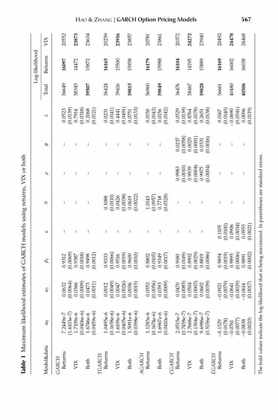
In this section, we examine the performance of the models estimated in fittingVIX time series. Table 1 displays the maximum likelihood estimates and standarderrors of GARCH models. The last three columns report the log-likelihood values.Although the contributions from both returns and VIX as well as the total arereported, we maximize lnLR when only returns are used, lnLV when only VIXlevels are used and the total when both time series are used.

The most notable finding in Table 1 is that the equity risk premium increasessignificantly in the GARCH, TGARCH, and CGARCH models when the VIX data isconsidered, especially when it is used alone. It increases from 0.0523 (returns used)to 0.2068 (returns and VIX used) and 0.7914 (VIX used) in the GARCH model, from0.0231 (returns used) to 0.0751 (returns and VIX used) and 0.4441 (VIX used) in theTGARCH model, and from 0.0529 (returns used) to 0.2651 (returns and VIX used)and 0.8764 (VIX used) in the CGARCH model. In the AGARCH model, it slightly


HAO & ZHANG | GARCH Option Pricing Models 567Ta

ble

1M

axim

umlik

elih

ood

esti

mat

esof

GA

RC

Hm

odel

sus

ing

retu

rns,

VIX

orbo

th

Log-

likel

ihoo

d

Mod

el&

data

α0

α1

β1

κθ

ρφ

λTo

tal

Ret

urns

VIX

GA

RC

HR

etur

ns7.

2449

e-7

0.06

320.

9312

––

––

0.05

2336

649

1609

720

552

(1.6

103e

-7)

(0.0

064)

(0.0

069)

(0.0

139)

VIX

1.71

09e-

60.

0366

0.93

87–

––

–0.

7914

3834

514

472

2387

3(0.0

406e

-6)

(0.0

009)

(0.0

018)

(0.0

318)

Both

1.67

46e-

60.

0473

0.94

98–

––

–0.

2068

3950

715

872

2363

4(0.0

459e

-6)

(0.0

011)

(0.0

012)

(0.0

121)

TGA

RC

HR

etur

ns1.

0495

e-6

0.00

120.

9333

–0.

1088

––

0.02

3136

424

1616

520

259

(0.1

658e

-6)

(0.0

049)

(0.0

066)

(0.0

110)

(0.0

141)

VIX

1.61

09e-

60.

0047

0.95

16–

0.04

26–

–0.

4441

3941

615

500

2391

6(0.0

405e

-6)

(0. 0

026)

(0.0

019)

(0.0

038)

(0.0

491)

Both

1.50

91e-

60.

0036

0.96

00–

0.06

19–

–0.

0751

3981

515

958

2385

7(0.0

398e

-6)

(0.0

015)

(0.0

010)

(0.0

022)

(0.0

133)

AG

AR

CH

Ret

urns

1.12

83e-

60.

0552

0.88

02–

1.01

43–

–0.

0150

3696

016

179

2078

1(0.1

674e

-6)

(0.0

056)

(0.0

105)

(0.0

957)

(0.0

142)

Both

1.69

67e-

60.

0393

0.93

49–

0.77

18–

–0.

0156

3984

915

988

2386

1(0.0

410e

-6)

(0.0

009)

(0.0

017)

(0.0

328)

(0.0

142)

CG

AR

CH

Ret

urns

2.05

15e-

70.

0470

0.91

80–

–0.

9983

0.02

370.

0529

3647

616

104

2037

2(0.7

458e

-7)

(0.0

085)

(0.0

149)

(0.0

010)

(0.0

058)

(0.0

139)

VIX

2.76

68e-

70.

0504

0.89

02–

–0.

9939

0.00

290.

8764

3846

714

195

2427

2(0.1

304e

-7)

(0.0

003)

(0.0

029)

(0.0

004)

(0.0

001)

(0.0

178)

Both

9.69

86e-

70.

0602

0.88

19–

–0.

9975

0.03

310.

2651

3982

815

889

2394

0(0.5

156e

-7)

(0.0

039)

(0.0

086)

(0.0

004)

(0.0

016)

(0.0

138)

EG

AR

CH

Ret

urns

−0.1

329

−0.0

921

0.98

540.

1105

––

–0.

0167

3666

116

169

2049

2(0.0

178)

(0.0

079)

(0.0

019)

(0.0

100)

(0.0

140)

VIX

−0.0

761

−0.0

641

0 .98

950.

0906

––

–−0.0

690

4048

016

002

2447

8(0.0

077)

(0.0

029)

(0.0

006)

(0.0

034)

(0.0

541)

Both

−0.0

838

−0.0

614

0.98

910.

0955

––

–0.

0096

4050

616

038

2446

8(0.0

020)

(0.0

017)

(0.0

002)

(0.0

021)

(0.0

119)

The

bold

valu

esin

dica

teth

elo

g-lik

elih

ood

that

isbe

ing

max

imiz

ed.I

npa

rent

hese

sar

est

anda

rder

rors

.



increases from 0.0150 to 0.0156 (returns and VIX used).10 However, the equity riskpremium is not significantly different from zero no matter which data set is usedin the EGARCH model.11 It can also be seen that in all models except the CGARCHmodel the persistence of conditional variance, β1, increases. This helps to raisethe long-run variance of the risk-neutral SR-SARV(1) process in together with theincrease in λ. The log-likelihood values indicate that more weights are attached tothe VIX data when both returns and VIX are used, which will also be confirmed byTable 2.

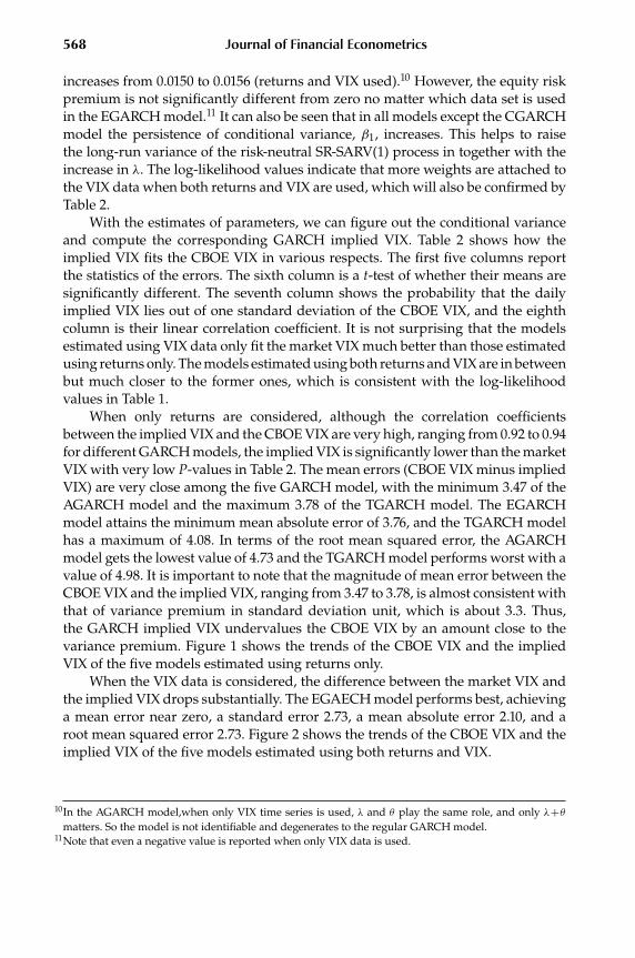
With the estimates of parameters, we can figure out the conditional varianceand compute the corresponding GARCH implied VIX. Table 2 shows how theimplied VIX fits the CBOE VIX in various respects. The first five columns reportthe statistics of the errors. The sixth column is a t-test of whether their means aresignificantly different. The seventh column shows the probability that the dailyimplied VIX lies out of one standard deviation of the CBOE VIX, and the eighthcolumn is their linear correlation coefficient. It is not surprising that the modelsestimated using VIX data only fit the market VIX much better than those estimatedusing returns only. The models estimated using both returns and VIX are in betweenbut much closer to the former ones, which is consistent with the log-likelihoodvalues in Table 1.

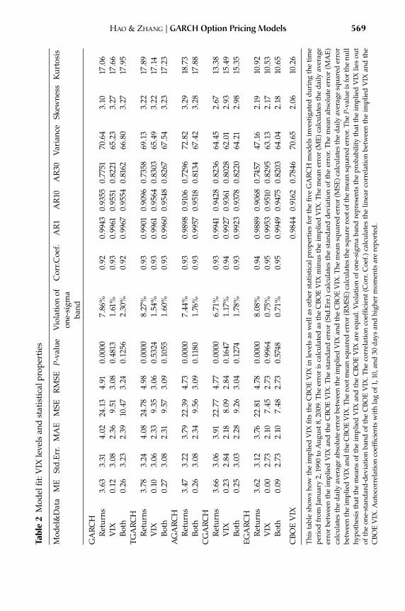
When only returns are considered, although the correlation coefficientsbetween the implied VIX and the CBOE VIX are very high, ranging from 0.92 to 0.94for different GARCH models, the implied VIX is significantly lower than the marketVIX with very low P-values in Table 2. The mean errors (CBOE VIX minus impliedVIX) are very close among the five GARCH model, with the minimum 3.47 of theAGARCH model and the maximum 3.78 of the TGARCH model. The EGARCHmodel attains the minimum mean absolute error of 3.76, and the TGARCH modelhas a maximum of 4.08. In terms of the root mean squared error, the AGARCHmodel gets the lowest value of 4.73 and the TGARCH model performs worst with avalue of 4.98. It is important to note that the magnitude of mean error between theCBOE VIX and the implied VIX, ranging from 3.47 to 3.78, is almost consistent withthat of variance premium in standard deviation unit, which is about 3.3. Thus,the GARCH implied VIX undervalues the CBOE VIX by an amount close to thevariance premium. Figure 1 shows the trends of the CBOE VIX and the impliedVIX of the five models estimated using returns only.

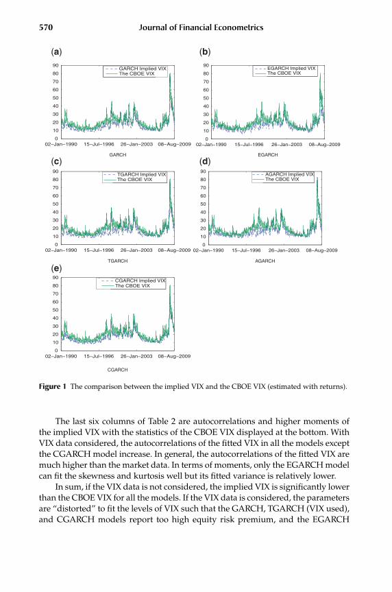
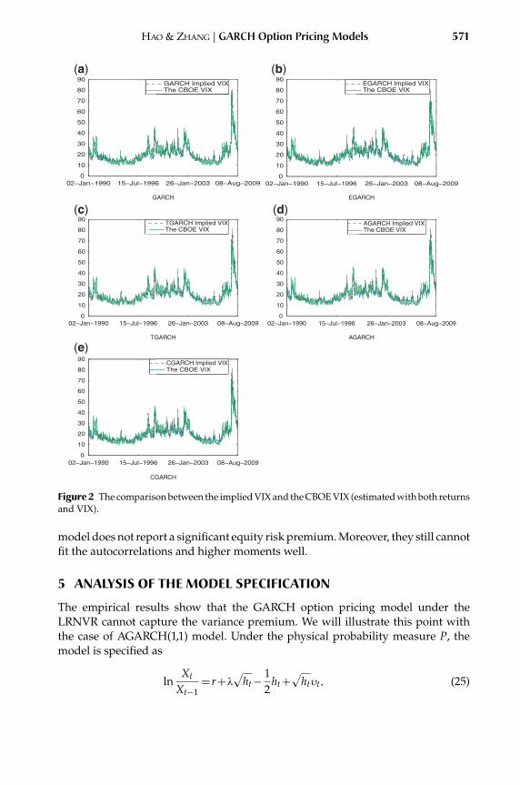
When the VIX data is considered, the difference between the market VIX andthe implied VIX drops substantially. The EGAECH model performs best, achievinga mean error near zero, a standard error 2.73, a mean absolute error 2.10, and aroot mean squared error 2.73. Figure 2 shows the trends of the CBOE VIX and theimplied VIX of the five models estimated using both returns and VIX.

10In the AGARCH model,when only VIX time series is used, λ and θ play the same role, and only λ+θmatters. So the model is not identifiable and degenerates to the regular GARCH model.

11Note that even a negative value is reported when only VIX data is used.


HAO & ZHANG | GARCH Option Pricing Models 569Ta

ble

2M

odel

fit:V

IXle

vels

and

stat

isti

calp

rope

rtie

s

Mod

el&

Dat

aM

ESt

d.Er

r.M

AE

MSE

RM

SEP

-val

ueV

iola

tion

ofon

e-si

gma

band

Cor

r.Coe

f.A

R1

AR

10A

R30

Var

ianc

eSk

ewne

ssK

urto

sis

GA

RC

HR

etur

ns3.

633.

314.

0224.1

34.

910.

0000

7.86

%0.

920.

9943

0.93

550.

7751

70.6

43.

1017.0

6V

IX0.

123.

082.

369.

513.

080.

4813

1.61

%0.

930.

9961

0.95

510.

8221

65.2

33.

2717.6

6Bo

th0.

263.

232.

3910.4

73.

240.

1256

2.30

%0.

920.

9967

0.95

540.

8162

66.8

03.

2717.9

5TG

AR

CH

Ret

urns

3.78

3.24

4.08

24.7

84.

980.

0000

8.27

%0.

930.

9901

0.90

960.

7358

69.1

33.

2217.8

9V

IX0.

103.

062.

339.

353.

060.

5324

1.54

%0.

930.

9961

0.95

640.

8303

65.4

93.

2217.1

4Bo

th0.

273.

082.

319.

573.

090.

1055

1.60

%0.

930.

9960

0.95

480.

8267

67.5

43.

2317.2

3A

GA

RC

HR

etur

ns3.

473.

223.

7922.3

94.

730.

0000

7.44

%0.

930.

9898

0.91

060.

7296

72.8

23 .

2918.7

3Bo

th0.

263.

082.

349.

563.

090.

1180

1.76

%0.

930.

9957

0.95

180.

8134

67.4

23.

2817.8

8C

GA

RC

HR

etur

ns3.

663.

063.

9122.7

74.

770.

0000

6.71

%0.

930.

9941

0.94

280.

8236

64.4

52.

6713.3

8V

IX0.

232.

842.

188.

092.

840.

1647

1.17

%0.

940.

9927

0.93

610.

8028

62.0

12.

9315.4

9Bo

th0.

253.

032.

289.

263 .

040.

1274

1.78

%0.

930.

9923

0.93

780.

8220

64.2

12.

9815.3

5EG

AR

CH

Ret

urns

3.62

3.12

3.76

22.8

14.

780.

0000

8.08

%0.

940.

9889

0.90

680.

7457

47.1

62.

1910.9

2V

IX0.

002.

732.

107.

452.

730.

9964

0.75

%0.

950.

9953

0.95

100.

8295

63.1

32.

1710.5

3Bo

th0.

092.

732.

107.

482.

730.

5748

0.71

%0.

950.

9949

0.94

750.

8203

64.0

42.

1810.6

5

CBO

EV

IX0.

9844

0.91

620.

7846

70.6

52.

0610.2

6

This

tabl

esh

ows

how

the

impl

ied

VIX

fits

the

CBO

EV

IXin

leve

lsas

wel

las

othe

rst

atis

tica

lpro

pert

ies

for

the

five

GA

RC

Hm

odel

sin

vest

igat

eddu

ring

the

tim

epe

riod

from

Janu

ary

2,19

90to

Aug

ust8

,200

9.Th

eer

ror

isca

lcul

ated

asth

eC

BOE

VIX

min

usth

eim

plie

dV

IX.T

hem

ean

erro

r(M

E)ca

lcul

ates

the

daily

aver

age

erro

rbe

twee

nth

eim

plie

dV

IXan

dth

eC

BOE

VIX

.The

stan

dard

erro

r(S

td.E

rr.)

calc

ulat

esth

est

anda

rdde

viat

ion

ofth

eer

ror.

The

mea

nab

solu

teer

ror

(MA

E)ca

lcul

ates

the

daily

aver

age

abso

lute

erro

rbe

twee

nth

eim

plie

dV

IXan

dth

eC

BOE

VIX

.The

mea

nsq

uare

der

ror

(MSE

)cal

cula

tes

the

daily

aver

age

squa

red

erro

rbe

twee

nth

eim

plie

dV

IXan

dth

eC

BOE

VIX

.The

root

mea

nsq

uare

der

ror

(RM

SE)c

alcu

late

sth

esq

uare

root

ofth

em

ean

squa

red

erro

r.Th

eP

-val

ueis

for

the

null

hypo

thes

isth

atth

em

eans

ofth

eim

plie

dV

IXan

dth

eC

BOE

VIX

are

equa

l.V

iola

tion

ofon

e-si

gma

band

repr

esen

tsth

epr

obab

ility

that

the

impl

ied

VIX

lies

out

ofth

eon

e-st

anda

rd-d

evia

tion

band

ofth

eC

BOE

VIX

.The

corr

elat

ion

coef

ficie

nt(C

orr.

Coe

f.)ca

lcul

ates

the

linea

rco

rrel

atio

nbe

twee

nth

eim

plie

dV

IXan

dth

eC

BOE

VIX

.Aut

ocor

rela

tion

coef

ficie

nts

wit

hla

gof

1,10

,and

30da

ysan

dhi

gher

mom

ents

are

repo

rted

.



02−Jan−1990 15−Jul−1996 26−Jan−2003 08−Aug−20090

10

20

30

40

50

60

70

80

90GARCH Implied VIXThe CBOE VIX

GARCH

02−Jan−1990 15−Jul−1996 26−Jan−2003 08−Aug−20090

10

20

30

40

50

60

70

80

90EGARCH Implied VIXThe CBOE VIX

EGARCH

02−Jan−1990 15−Jul−1996 26−Jan−2003 08−Aug−20090

10

20

30

40

50

60

70

80

90TGARCH Implied VIXThe CBOE VIX

TGARCH

02−Jan−1990 15−Jul−1996 26−Jan−2003 08−Aug−20090

10

20

30

40

50

60

70

80

90AGARCH Implied VIXThe CBOE VIX

AGARCH

02−Jan−1990 15−Jul−1996 26−Jan−2003 08−Aug−20090

10

20

30

40

50

60

70

80

90CGARCH Implied VIXThe CBOE VIX

CGARCH

(a) (b)

(c) (d)

(e)

Figure 1 The comparison between the implied VIX and the CBOE VIX (estimated with returns).

The last six columns of Table 2 are autocorrelations and higher moments ofthe implied VIX with the statistics of the CBOE VIX displayed at the bottom. WithVIX data considered, the autocorrelations of the fitted VIX in all the models exceptthe CGARCH model increase. In general, the autocorrelations of the fitted VIX aremuch higher than the market data. In terms of moments, only the EGARCH modelcan fit the skewness and kurtosis well but its fitted variance is relatively lower.

In sum, if the VIX data is not considered, the implied VIX is significantly lowerthan the CBOE VIX for all the models. If the VIX data is considered, the parametersare “distorted” to fit the levels of VIX such that the GARCH, TGARCH (VIX used),and CGARCH models report too high equity risk premium, and the EGARCH



02−Jan−1990 15−Jul−1996 26−Jan−2003 08−Aug−20090

10

20

30

40

50

60

70

80

90GARCH Implied VIXThe CBOE VIX

GARCH

02−Jan−1990 15−Jul−1996 26−Jan−2003 08−Aug−20090

10

20

30

40

50

60

70

80

90EGARCH Implied VIXThe CBOE VIX

EGARCH

02−Jan−1990 15−Jul−1996 26−Jan−2003 08−Aug−20090

10

20

30

40

50

60

70

80

90TGARCH Implied VIXThe CBOE VIX

TGARCH

02−Jan−1990 15−Jul−1996 26−Jan−2003 08−Aug−20090

10

20

30

40

50

60

70

80

90AGARCH Implied VIXThe CBOE VIX

AGARCH

02−Jan−1990 15−Jul−1996 26−Jan−2003 08−Aug−20090

10

20

30

40

50

60

70

80

90CGARCH Implied VIXThe CBOE VIX

CGARCH

(a) (b)

(c) (d)

(e)

Figure 2 The comparison between the implied VIX and the CBOE VIX (estimated with both returnsand VIX).

model does not report a significant equity risk premium. Moreover, they still cannotfit the autocorrelations and higher moments well.

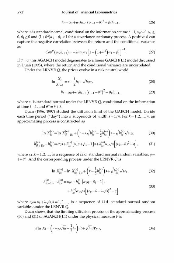
5 ANALYSIS OF THE MODEL SPECIFICATION

The empirical results show that the GARCH option pricing model under theLRNVR cannot capture the variance premium. We will illustrate this point withthe case of AGARCH(1,1) model. Under the physical probability measure P, themodel is specified as

lnXt

Xt−1=r+λ

√ht − 1

2ht +

√htυt, (25)



ht =α0 +α1ht−1(υt−1 −θ)2 +β1ht−1, (26)

whereυt is standard normal, conditional on the information at time t−1;α0>0,α1 ≥0,β1 ≥0 and (1+θ2)α1 +β1<1 for a covariance stationary process. A positive θ cancapture the negative correlation between the return and the conditional varianceas

CovP(υt,ht+1)=−2θα0α1

[1−

(1+θ2

)α1 −β1

]−1. (27)

If θ=0, this AGARCH model degenerates to a linear GARCH(1,1) model discussedin Duan (1995), where the return and the conditional variance are uncorrelated.

Under the LRNVR Q, the prices evolve in a risk neutral world

lnXt

Xt−1=r− 1

2ht +

√htεt, (28)

ht =α0 +α1ht−1(εt−1 −θ∗)2 +β1ht−1, (29)

where εt is standard normal under the LRNVR Q, conditional on the informationat time t−1, and θ∗ =θ+λ.

Duan (1996, 1997) studied the diffusion limit of the GARCH model. Divideeach time period (“day”) into n subperiods of width s=1/n. For k =1,2,...,n, anapproximating process is constructed as

ln X(n)ks = ln X(n)

(k−1)s +(

r+λ√

h(n)ks − 1

2h(n)

ks

)s+

√h(n)

ks

√sυk, (30)

h(n)(k+1)s −h(n)

ks =α0s+h(n)ks

[α1q+β1 −1

]s+h(n)

ks α1√

s[(υk −θ)2 −q

], (31)

where υk,k =1,2,..., is a sequence of i.i.d. standard normal random variables; q=1+θ2. And the corresponding process under the LRNVR Q is

ln X(n)ks = ln X(n)

(k−1)s +(

r− 12

h(n)ks

)s+

√h(n)

ks

√sεk, (32)

h(n)(k+1)s −h(n)

ks =α0s+h(n)ks

[α1q+β1 −1

]s

+h(n)ks α1

√s[(εk −θ−λ√s

)2 −q],

(33)

where εk =υk +λ√s,k =1,2,..., is a sequence of i.i.d. standard normal randomvariables under the LRNVR Q.

Duan shows that the limiting diffusion process of the approximating process(30) and (31) of AGARCH(1,1) under the physical measure P is

dln Xt =(

r+λ√

ht − 12

ht

)dt+

√htdW1t, (34)



dht =[α0 +(

α1q+β1 −1)ht]dt−2θα1htdW1t +

√2α1htdW2t, (35)

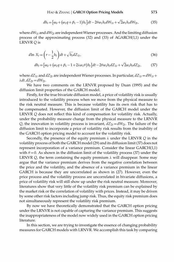
where dW1t and dW2t are independent Wiener processes. And the limiting diffusionprocess of the approximating process (32) and (33) of AGARCH(1,1) under theLRNVR Q is

dln Xt =(

r− 12

ht

)dt+

√htdZ1t, (36)

dht =[α0 +(

α1q+β1 −1+2λα1θ)ht]dt−2θα1htdZ1t +

√2α1htdZ2t, (37)

where dZ1t and dZ2t are independent Wiener processes. In particular, dZ1t =dW1t +λdt,dZ2t =dW2t.

We have two comments on the LRNVR proposed by Duan (1995) and thediffusion limit properties of the GARCH model.

Firstly, for the true bivariate diffusion model, a price of volatility risk is usuallyintroduced to the volatility process when we move from the physical measure tothe risk neutral measure. This is because volatility has its own risk that has tobe compensated. However, the diffusion limit of the GARCH model under theLRNVR Q does not reflect this kind of compensation for volatility risk. Actually,under the probability measure change from the physical measure to the LRNVRQ, the innovation in volatility process is invariant, dZ2t =dW2t. The failure of thediffusion limit to incorporate a price of volatility risk results from the inability ofthe GARCH option pricing model to account for the volatility risk.

Secondly, the presence of the equity premium λ under the LRNVR Q in thevolatility process of both the GARCH model (29) and its diffusion limit (37) does notrepresent incorporation of a variance premium. Consider the linear GARCH(1,1)with θ=0. As shown in the diffusion limit of the volatility process (37) under theLRNVR Q, the term containing the equity premium λ will disappear. Some mayargue that the variance premium derives from the negative correlation betweenthe price and the volatility, and the absence of a variance premium in the linearGARCH is because they are uncorrelated as shown in (27). However, even theprice process and the volatility process are uncorrelated in bivariate diffusions, aprice of volatility risk will still show up under the risk neutral measure. Moreover,literatures show that very little of the volatility risk premium can be explained bythe market risk or the correlation of volatility with prices. Instead, it may be drivenby some other risk factors including jump risk. Thus, the equity risk premium doesnot simultaneously represent the volatility risk premium.

By now we have theoretically demonstrated that the GARCH option pricingunder the LRNVR is not capable of capturing the variance premium. This suggeststhe inappropriateness of the model now widely used in the GARCH option pricingliterature.

In this section, we are trying to investigate the essence of changing probabilitymeasures for GARCH models with LRNVR. We accomplish this task by comparing



the continuous-time limits of the GARCH processes under physical and the risk-neutral measures. We demonstrate our logic by using the diffusion limit of GARCHmodels in Duan (1996, 1997). Similar analysis can be done with Heston and Nandi(2000). By comparing the continuous-time limits instead of GARCH processesthemselves, we can easily find out what is happening during the process ofchanging probability measures. In continuous-time model, we have an adjustmentof equity risk premium for the innovation in the return process and anotheradjustment of variance risk premium for the innovation in the variance process,as demonstrated in Wiggins (1987), Johnson and Shanno (1987), Hull and White(1987), Scott (1987), and Heston (1993). However, when we look at the continuous-time limits of the GARCH processes, we find that there is only one risk adjustmentfor the innovation in returns, and the innovations in the variance process are thesame under both physical and risk-neutral measures. We then argue that there isno risk adjustment for the variance risk when changing the GARCH process fromphysical to the risk-neutral measures.

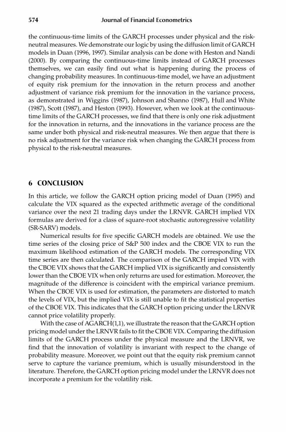
6 CONCLUSION

In this article, we follow the GARCH option pricing model of Duan (1995) andcalculate the VIX squared as the expected arithmetic average of the conditionalvariance over the next 21 trading days under the LRNVR. GARCH implied VIXformulas are derived for a class of square-root stochastic autoregressive volatility(SR-SARV) models.

Numerical results for five specific GARCH models are obtained. We use thetime series of the closing price of S&P 500 index and the CBOE VIX to run themaximum likelihood estimation of the GARCH models. The corresponding VIXtime series are then calculated. The comparison of the GARCH impied VIX withthe CBOE VIX shows that the GARCH implied VIX is significantly and consistentlylower than the CBOE VIX when only returns are used for estimation. Moreover, themagnitude of the difference is coincident with the empirical variance premium.When the CBOE VIX is used for estimation, the parameters are distorted to matchthe levels of VIX, but the implied VIX is still unable to fit the statistical propertiesof the CBOE VIX. This indicates that the GARCH option pricing under the LRNVRcannot price volatility properly.

With the case of AGARCH(1,1), we illustrate the reason that the GARCH optionpricing model under the LRNVR fails to fit the CBOE VIX. Comparing the diffusionlimits of the GARCH process under the physical measure and the LRNVR, wefind that the innovation of volatility is invariant with respect to the change ofprobability measure. Moreover, we point out that the equity risk premium cannotserve to capture the variance premium, which is usually misunderstood in theliterature. Therefore, the GARCH option pricing model under the LRNVR does notincorporate a premium for the volatility risk.



The empirical results and the theoretical arguments both indicate that theGARCH option pricing model under the LRNVR is not capable of capturing thevariance premium. This suggests that the LRNVR is not completely specified, andkind of fully risk neutral measure for the GARCH option pricing is called for.

It is an interesting topic to establish an equilibrium GARCH option pric-ing model that is able to incorporate Christoffersen, Heston, and Jacobs’ (2011)variance-dependent pricing kernel. Zhang, Zhao, and Chang’s (2012) production-based general equilibrium is a possible setup to develop the model.

APPENDIX

A. PROOFS

Proof of Proposition 1. For k ≥1,

EQt(ft+k

)=e′EQt(Ft+k

)=e′EQt(+�Ft+k−1 +Vt+k

)=e′EQ

t

[+EQ

t+k−1

(�Ft+k−1 +Vt+k

)]=e′EQ

t(+�Ft+k−1

)=e′[+�EQ

t(Ft+k−1

)],

(A1)

and continuing this iterating process, we have

EQt(ft+k

)=e′⎛⎝k−1∑

i=0

�i+�kFt

⎞⎠. (A2)

With Vixt = 1n∑n

k=1EQt (ht+k)= 1

n∑n−1

k=0 EQt (ft+k), we have

Vixt =ζ+ Ft, (A3)

with

ζ = e′

n

n−1∑k=1

k−1∑i=0

�i,

= e′

n

n−1∑k=1

�k,

which is affine in Ft.



For p=1, we can get VIXt as a linear function of the conditional variance of thenext period, ft,

Vixt =ζ+ψ ft, (A4)

where

ζ =

1−� (1−ψ),

ψ= 1−�n

n(1−�).

�

Proof of Proposition 2. Let ut =ξt/√

ht. The results for GARCH(1,1) and AGARCH(1,1)have been proved in Proposition 3.2 of Meddahi and Renault (2004). Following thesame idea, we rewrite the first three models as ht =ω+γ ht−1 +vt−1 with:

GARCH(1,1): ω=α0, γ =α1(1+λ2)+β1, vt−1 =α1ht−1(u2t−1 −1−2λut−1).

TARCH(1,1): ω=α0, γ =α1(1+λ2)+β1 +θS, vt−1 =α1ht−1(u2t−1 −1−2λut−1)+

θht−1[(ut−1 −λ)21(ut−1<λ)−S], where S=EQt−1[(ut −λ)21(ut<λ)].

AGARCH(1,1): ω=α0, γ =α1[1+(λ+θ )2]+β1, vt−1 =α1ht−1[u2t−1 −1−2(λ+

θ )ut−1].

We can rewrite the CGARCH(1,1) model as ht =e′Ft and Ft =+�Ft−1 +Vt−1

with: e=(

10

), Ft =

(htqt

), =α0

(11

), �=

(α1 +β1 +(φ+α1)λ2 ρ−α1 −β1

φλ2 ρ

), Vt =

ht−1(u2t−1 −2λut−1 −1)

(φ+α1φ

).

Since EQt−2(ut−1)=0 and EQ

t−2(u2t−1)=1, we have EQ

t−2(vt−1)=0 and EQt−2(Vt−1)=

0. Thus, ξt is a SR-SARV(1) for the first three models and a SR-SARV(2) for theCGARCH model. �

Proof of Proposition 3. Denote eγiωEQ

t (eγivt+1 )= ιi. Under the LRNVR Q, the expectation

of the conditional variance k ≥1 periods ahead can be expressed as

EQt(ft+k

)=eωEQt

[EQ

t+k−1

(f γt+k−1evt+k

)]=eωEQ

t+k−1

(evt+k

)EQ

t

(f γt+k−1

)= ι0EQ

t

(f γt+k−1

).

(A5)

For 0≤ i≤k−1, we have

γ i lnft+k−i =γ iω+γ i+1 lnft+k−i−1 +γ ivt+k−i. (A6)



Thus,

EQt

(f γ

i

t+k−i

)=eγ

iωEQt

(f γ

i+1

t+k−i−1

)EQ

t+k−i−1

(eγ

ivt+k−i)

= ιiEQt

(f γ

i+1

t+k−i−1

).

(A7)

Then starting from formula (A5) and iterating with formula (A7), we have

EQt (ft+k)= f γ

k

t

k−1∏i=0

ιi. (A8)

And the implied VIX formula is

Vixt = 1n

⎡⎣ft +

n−1∑k=1

⎛⎝k−1∏

i=0

ιi

⎞⎠f γ

k

t

⎤⎦. (A9)

�

B. IMPLIED VIX FORMULAS

Substituting their parameters into the general formula (11), we get the followingVIX formulas:GARCH(1,1):

Vixt =A+Bht+1, (A10)

where

A= α0

1−η (1−B),

B= 1−ηn

n(1−η),

η=α1

(1+λ2

)+β1.

TGARCH(1,1):Vixt =C+Dht+1, (A11)

where

C= α0

1−η (1−D),

D= 1−ηn

n(1−η),



η=α1

(1+λ2

)+β1 +θS.

If ut =ξt/√

ht follows i.i.d. N(0,1), S=[λ√2π

e− λ22 +(1+λ2)N(λ)

].

AGARCH(1,1):Vixt =E+Fht+1, (A12)

where

E= α0

1−η (1−F),

F= 1−ηn

n(1−η),

η=α1

[1+(λ+θ)2

]+β1.

CGARCH(1,1):For CGARCH(1,1), we cannot give an explicit formula, but we can refer to

equations (7) and (A2) to get the result numerically.EGARCH(1,1):

For EGARCH(1,1), the ιi in (A9) is given by ιi =eβi1α0 EQ

t (eβi1g(ut+1−λ)).

If ut is i.i.d. standard normal, then

ιi =eβi1(α0−κ

√2/π )

{e−β i

1(α1−κ)λ+ [βi1(α1−κ)]2

2 N[λ−β i

1(α1 −κ)]

+e−β i1(α1+κ)λ+ [βi

1(α1+κ)]22 N

[β i

1(α1 +κ)−λ]}.(A13)

Received May 6, 2010; revised December 3, 2012; accepted December 6, 2012.

REFERENCES

Andersen, T. G., T. Bollerslev, F. X. Diebold, and P. Labys. 2003. Modeling andForecasting Realized Volatility. Econometrica 71: 579–625.

Bakshi, G., and N. Kapadia. 2003. Delta-Hedged Gains and the Negative MarketVolatility Risk Premium. Review of Financial Studies 16: 527–566.

Barone-Adesi, G., R. Engle, and L. Mancini. 2008. A GARCH Option Pricing Modelwith Filtered Historical Simulation. Review of Financial Studies 21: 1223–1258.

Bollerslev, T. 1986. Generalized Autoregressive Conditional Heteroskedasticity.Journal of Econometrics 31: 307–327.

Carr, P., and L.-R. Wu. 2009. Variance Risk Premiums. Review of Financial Studies 22:1311–1341.



Chernov, M., and E. Ghysels. 2000. A Study towards a Unified Approach to the JointEstimation of Objective and Risk Neutral Measures for the Purpose of OptionValuation. Journal of Financial Economics 56: 407–458.

Christoffersen, P., R. Elkamhi, B. Feunou, and K. Jacobs. 2010. Option Valuation withConditional Heteroskedasticity and Nonnormality. Review of Financial Studies23: 2139–2183.

Christoffersen, P., S. Heston, and K. Jacobs. 2006. Option Valuation with ConditionalSkewness. Journal of Econometrics 131: 253–284.

Christoffersen, P., S. Heston, and K. Jacobs. 2011. “Capturing Option Anomalieswith a Variance-Dependent Pricing Kernel.” Working Paper. Available atSSRN: http://ssrn.com/abstract=1538394

Christoffersen, P., and K. Jacobs. 2004. Which GARCH Model for Option Valuation?Management Science 50: 1204–1221.

Christoffersen, P., K. Jacobs, C. Ornthanalai, and Y.-T. Wang. 2008. Option Valuationwith Long-run and Short-run Volatility Components. Journal of FinancialEconomics 90: 272–297.

Coval, J. D., and T. Shumway. 2001. Expected Option Returns. Journal of Finance 56:983–1009.

Duan, J.-C. 1995. The GARCH Option Pricing Model. Mathematical Finance 5: 13–32.Duan, J.-C. 1996. “A Unified Theory of Option Pricing under Stochastic Volatility-

from GARCH to Diffusion.” Working paper, Hong Kong University of Scienceand Technology.

Duan, J.-C. 1997. Augmented GARCH(p, q) Process and its Diffusion Limit. Journalof Econometrics 79: 97–127.

Duan, J.-C. 1999. “Conditionally Fat-Tailed Distributions and the Volatility Smile inOptions.” Working Paper, University of Toronto.

Demeterfi, K., E. Derman, M. Kamal, and J. Zou. 1999. A Guide to Volatility andVariance Swaps. Journal of Derivatives 6: 9–32.

Engle, R. 1982. Autoregressive Conditional Heteroskedasticity with Estimates ofthe Variance of U.K. Inflation. Econometrica 50: 987–1008.

Engle, R., and G. Lee. 1993. “A Permanent and Transitory Component Model ofStock Return Volatility.” Working paper 92-44R, University of California, SanDiego.

Engle, R., and V. Ng. 1993. Measuring and Testing the Impact of News on Volatility.Journal of Finance 48: 1749–1778.

Eraker, B. 2008. “The Volatility Premium.” Working Paper, Duke University.Garcia, R., and É. Renault. 1998. A Note on Hedging in ARCH and Stochastic

Volatility Option Pricing Models. Mathematical Finance 8: 153–161.Garcia, R., E. Ghysels, and É. Renault. 2010. “Econometrics of Option Pricing

Models.” In Y. Aït-Sahalia and L. P. Hansen (eds.), Handbook of FinancialEconometrics, Vol. 1. Amsterdam: North Holland.

Glosten, L., R. Jagannathan, and D. Runkle. 1993. On the Relation between theExpected Value and the Volatility of the Nominal Excess Return on Stocks.Journal of Finance 48: 1779–1801.



Heston, S. 1993. A Closed Form Solution for Options with Stochastic Volatilitywith Applications to Bond and Currency Options. Review of Financial Studies6: 327–343.

Heston, S., and S. Nandi. 2000. A Closed-Form GARCH Option Valuation Model.Review of Financial Studies 13: 585–625.

Hull, J., and A. White. 1987. The Pricing of Options on Assets with StochasticVolatilities. Journal of Finance 42: 281–300.

Johnson, H., and D. Shanno. 1987. Option Pricing When the Variance is Changing.Journal of Financial Quantitative Analysis 22: 143–151.

Jones, C. S. 2003. The Dynamics of Stochastic Volatility Evidence from Underlyingand Option Markets. Journal of Econometrics 116: 181–224.

Kallsen, J., and M. Taqqu. 1998. Option Pricing in ARCH-Type Models. MathematicalFinance 8: 13–26.

Meddahi, N., and E. Renault. 2004. Temporal Aggregation of Volatility Models.Journal of Econometrics 119: 355–379.

Nelson, D. 1991. Conditional Heteroskedasticity in Asset Returns: A NewApproach. Econometrica 59: 347–370.

Pan, J. 2002. The Jump-Risk Premia Implicit in Options: Evidence from an IntegratedTime-Series Study. Journal of Financial Economics 63: 3–50.

Ritchken, P., and R. Trevor. 1999. Pricing Options under Generalized GARCH andStochastic Volatility Processes. Journal of Finance 54: 377–402.

Scott, L. 1987. Option Pricing When the Variance Changes Randomly: Theory,Estimation, and an Application. Journal of Financial Quantitative Analysis 22:419–438.

Siu, T. K., H. Tong, and H.-L. Yang. 2004. On Pricing Derivatives under GARCHModels: A Dynamic Gerber-Shiu Approach. North American Actuarial Journal8: 17–31.

Todorov, V. 2010. Variance Risk-Premium Dynamics: The Role of Jumps. Review ofFinancial Studies 23: 345–383.

Vilkov, G. 2008. “Variance Risk Premium Demystified.” Working Paper, GoetheUniversity.

Wiggins, J. 1987. Option Values under Stochastic Volatility: Theory and EmpiricalEstimates. Journal of Finance 19: 351–372.

Zhang, J. E., H.-M. Zhao, and E. C. Chang. 2012. Equilibrium Asset and OptionPricing under Jump Diffusion. Mathematical Finance 22: 538–568.

Copyright of Journal of Financial Econometrics is the property of Oxford University Press /USA and its content may not be copied or emailed to multiple sites or posted to a listservwithout the copyright holder's express written permission. However, users may print,download, or email articles for individual use.

Documents

GARCH Option Pricing Models, the CBOE VIX, and Variance ... · PDF filepapers discussing the weakness of traditional GARCH option pricing models. Garcia and Renault ... for both the