Embed Size (px)
Citation preview

Option PricingOption Pricing..

Stochastic ProcessStochastic Process
A variable whose value changes A variable whose value changes over time in an uncertain way is said over time in an uncertain way is said to follow a stochastic process. to follow a stochastic process.
Stochastic processes can be Stochastic processes can be “discrete time” or “continuous “discrete time” or “continuous time” and also “discrete variable” time” and also “discrete variable” or “continuous variable”or “continuous variable”

Markov ProcessMarkov Process
It is a particular type of stochastic process It is a particular type of stochastic process where only the present value of a variable is where only the present value of a variable is relevant for predicting the future. The past relevant for predicting the future. The past history of the variable and the way in which history of the variable and the way in which the present value has emerged from the past the present value has emerged from the past are irrelevant.are irrelevant.
It is consistence with the weak form of market It is consistence with the weak form of market efficiency and means that while statistical efficiency and means that while statistical properties of the stock prices may be useful in properties of the stock prices may be useful in determining the characteristics of the determining the characteristics of the stochastic process followed by the stock price stochastic process followed by the stock price but the particular path followed in the past is but the particular path followed in the past is irrelevant.irrelevant.

Wiener ProcessWiener Process
It is a particular type of Markov Stochastic It is a particular type of Markov Stochastic Process and has been used in physics to Process and has been used in physics to describe the motion of a particular subjected describe the motion of a particular subjected to a large number of small molecular shocks to a large number of small molecular shocks and is sometimes referred to as Brownian and is sometimes referred to as Brownian Motion. It has two properties;Motion. It has two properties;
1.1. Small change is equal to root of change Small change is equal to root of change in time multiplied by a random variable in time multiplied by a random variable following a standardized normal distribution.following a standardized normal distribution.2.2. For two different short intervals, the For two different short intervals, the small changes are independent.small changes are independent.

Lognormal DistributionLognormal Distribution
It is the variable whose logarithm It is the variable whose logarithm values are normally distributed. values are normally distributed. We need to convert lognormal We need to convert lognormal distributions (stochastic stock distributions (stochastic stock price changes) to normal price changes) to normal distributions so that one could distributions so that one could undertake analysis using undertake analysis using confidence limits, hypothesis confidence limits, hypothesis testing etc. testing etc.

Option Pricing ModelsOption Pricing Models
DCF criterion cannot be used since risk DCF criterion cannot be used since risk of anof an
option is virtually indeterminate and option is virtually indeterminate and hencehence
the discount rate is impossible to bethe discount rate is impossible to be
estimated. The two popular models are:estimated. The two popular models are:
The Binomial ModelThe Binomial Model Black – Scholes ModelBlack – Scholes Model

The Binomial ModelThe Binomial Model
The model assumes,The model assumes,
The price of asset can only go up The price of asset can only go up or go down in fixed amounts in or go down in fixed amounts in discrete time.discrete time.
There is no arbitrage between There is no arbitrage between the option and the replicating the option and the replicating portfolio composed of underlying portfolio composed of underlying asset and risk-less asset.asset and risk-less asset.

The Binomial ModelThe Binomial Model
Current stock price = SCurrent stock price = S Next Year values = uS or dSNext Year values = uS or dS B amount can be borrowed at ‘r’. B amount can be borrowed at ‘r’.
Interest factor is (1+r) = RInterest factor is (1+r) = R d < R < u (no risk free arbitrage d < R < u (no risk free arbitrage
possible)possible) E is the exercise price E is the exercise price

The Binomial ModelThe Binomial Model
Depending on the change in stock Depending on the change in stock
value, option value will bevalue, option value will be
Cu = Max (uS – E, 0)Cu = Max (uS – E, 0)
Cd = Max (dS – E, 0)Cd = Max (dS – E, 0)

The Binomial ModelThe Binomial Model..
S
Su
Sd
Su2
Sud
Sd2

The Binomial ModelThe Binomial ModelWe now set a portfolio of ∆ shares and B We now set a portfolio of ∆ shares and B
amount ofamount ofdebt such that its payoff is equal to that of calldebt such that its payoff is equal to that of calloption after 1 year. Then, option after 1 year. Then,
Cu = ∆uS + RB……………Cu = ∆uS + RB…………… (1)(1)Cd = ∆dS + RB……………. Cd = ∆dS + RB……………. (2)(2)Solving these equations, Solving these equations, (Cu – Cd) (Cu – Cd)
∆ ∆ = = ; and ; and S(u-d)S(u-d)
(uCd – dCu)(uCd – dCu)
B = B = (u – d)R(u – d)R
Hence C = ∆S + B, since portfolio has same payoff asHence C = ∆S + B, since portfolio has same payoff ascall option.call option.

IllustrationIllustration
A stock is currently selling for Rs.40. A stock is currently selling for Rs.40. The call option on the stockThe call option on the stockexercisable a year from now at a strikeexercisable a year from now at a strikeprice of Rs.45 is currently selling atprice of Rs.45 is currently selling atRs.8. The risk-free rate is 10%. TheRs.8. The risk-free rate is 10%. Thestock can either rise or fall after a year.stock can either rise or fall after a year.It can fall by 20%. By what percentageIt can fall by 20%. By what percentagecan it rise?can it rise?

Black-Scholes Model as the Black-Scholes Model as the
Limit of the Binomial ModelLimit of the Binomial Model
The Binomial Model converges to the The Binomial Model converges to the Black-Black-
Scholes model as the number of timeScholes model as the number of time
periods increases.periods increases.

Black-Scholes Model: The Black-Scholes Model: The originorigin
1820s – Scottish scientist Robert Brown 1820s – Scottish scientist Robert Brown observed motion of suspended particles in observed motion of suspended particles in water.water.
Early 19Early 19thth century – Albert Einstein used century – Albert Einstein used Brownian motion to explain movements of Brownian motion to explain movements of molecules, many research papers.molecules, many research papers.
1900 – French scholar, Louis Bachelier 1900 – French scholar, Louis Bachelier wrote dissertation on option pricing and wrote dissertation on option pricing and developed a model strikingly similar to BSM.developed a model strikingly similar to BSM.
1951 – Japanese mathematician Kiyoshi Ito 1951 – Japanese mathematician Kiyoshi Ito developed Ito’s Lemma that was used in developed Ito’s Lemma that was used in option pricing.option pricing.

Black-Scholes Model: The Black-Scholes Model: The originorigin
Fischer Black and Myron Scholes worked in Fischer Black and Myron Scholes worked in Finance Faculty at MIT Published paper in Finance Faculty at MIT Published paper in 1973. They were later joined by Robert 1973. They were later joined by Robert Merton.Merton.
Fischer left academia in 1983, died in Fischer left academia in 1983, died in 1995 at 57.1995 at 57.
1997 – Scholes and Merton got Nobel Prize1997 – Scholes and Merton got Nobel Prize

Black-Scholes ModelBlack-Scholes Model Fischer Black and Myron Scholes, The Journal of Political Economy, Fischer Black and Myron Scholes, The Journal of Political Economy,
19731973
Assumptions:Assumptions: The underlying stock pays no dividends.The underlying stock pays no dividends. It is a European option.It is a European option. The stock price is continuous and is The stock price is continuous and is
distributed lognormally.distributed lognormally. There are no transaction costs and taxes.There are no transaction costs and taxes. No restrictions or penalty on short sellingNo restrictions or penalty on short selling The risk free rate is known and is constant The risk free rate is known and is constant
over the life of the option.over the life of the option.

Black-Scholes ModelBlack-Scholes Model
CC00 = S = S00 N (d N (d11) – E/e) – E/ertrt N (d N (d22) where,) where,
CC00 = Present equilibrium value of call option= Present equilibrium value of call option
SS00 = Current stock price= Current stock price
E E = Exercise price= Exercise price
e e = Base of natural logarithm= Base of natural logarithm
rr = Continuously compounded risk free interest = Continuously compounded risk free interest raterate
tt = length of time in years to expiration= length of time in years to expiration
N (*) N (*) = Cumulative probability distribution function of a= Cumulative probability distribution function of a standardized normal distributionstandardized normal distribution

Black-Scholes ModelBlack-Scholes Model
C = S N (dC = S N (d11) – K) – Kee-rt-rt N (d N (d22) where,) where,
CC = Present equilibrium value of call option= Present equilibrium value of call option
SS = Current stock price= Current stock price
KK = Exercise price= Exercise price
e e = Base of natural logarithm= Base of natural logarithm
rr = Continuously compounded risk free interest = Continuously compounded risk free interest raterate
tt = length of time in years to expiration= length of time in years to expiration
N (*) N (*) = Cumulative probability distribution function of = Cumulative probability distribution function of aa
standardized normal distributionstandardized normal distribution

Black-Scholes ModelBlack-Scholes Model
llnn (S (S00/E) + (r + ½ /E) + (r + ½ σσ22)t )t dd11 = =
σσ √t √t
llnn (S (S00/E) + (r - ½ /E) + (r - ½ σσ22)t )t dd22 = =
σσ √t √t
where lwhere lnn is the natural logarithm is the natural logarithm
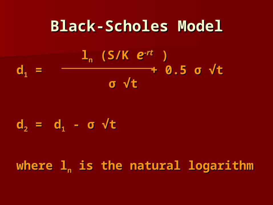
Black-Scholes ModelBlack-Scholes Model
llnn (S/K (S/K ee-rt-rt ))dd11 = = + 0.5 + 0.5 σ σ √t √t
σσ √t √t
dd22 = = dd11 - - σ σ √t √t
where lwhere lnn is the natural logarithm is the natural logarithm

IllustrationIllustration
The standard deviation of the continuously The standard deviation of the continuously
compounded stock price change for acompounded stock price change for a
company is estimated to be 20% per year.company is estimated to be 20% per year.
The stock currently sells for Rs.80 and theThe stock currently sells for Rs.80 and the
effective annual interest rate is Rs.15.03%.effective annual interest rate is Rs.15.03%.
What is the value of a one year call optionWhat is the value of a one year call option
on the stock of the company if the exerciseon the stock of the company if the exercise
price is Rs.82?price is Rs.82?
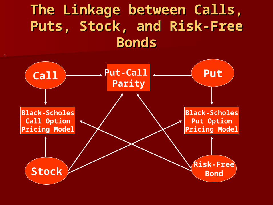
The Linkage between Calls, The Linkage between Calls, Puts, Stock, and Risk-Free Puts, Stock, and Risk-Free
BondsBonds..
Call
Stock
Put
Risk-FreeBond
Black-ScholesCall Option
Pricing Model
Put-Call Parity
Black-ScholesPut Option
Pricing Model

Put-Call Parity TheoremPut-Call Parity Theorem
Payoffs just before Payoffs just before expirationexpiration
If SIf S11< E< E If S If S11> E> E
1.1. Buy the equity stockBuy the equity stock S S11 S S11
2.2. Buy a put optionBuy a put option E-SE-S11 0 0
3.3. Borrow amount equal Borrow amount equal
to exercise priceto exercise price - E- E - E- E
1+2+3=Buy a call option1+2+3=Buy a call option 0 0 S S11- E- E
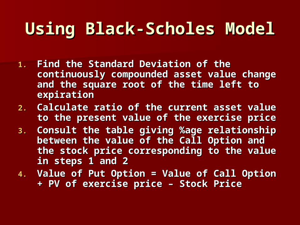
Using Black-Scholes ModelUsing Black-Scholes Model
1.1. Find the Standard Deviation of the Find the Standard Deviation of the continuously compounded asset value continuously compounded asset value change and the square root of the time change and the square root of the time left to expirationleft to expiration
2.2. Calculate ratio of the current asset value Calculate ratio of the current asset value to the present value of the exercise priceto the present value of the exercise price
3.3. Consult the table giving %age relationship Consult the table giving %age relationship between the value of the Call Option and between the value of the Call Option and the stock price corresponding to the value the stock price corresponding to the value in steps 1 and 2in steps 1 and 2
4.4. Value of Put Option = Value of Call Option Value of Put Option = Value of Call Option + PV of exercise price – Stock Price+ PV of exercise price – Stock Price

IllustrationIllustration
Find the value of a one year call option as Find the value of a one year call option as
well as a put option, if the current stockwell as a put option, if the current stock
price is Rs.120, exercise price is Rs.125 andprice is Rs.120, exercise price is Rs.125 and
the S.D. of continuously compounded pricethe S.D. of continuously compounded price
change of the stock is 30%. The effectivechange of the stock is 30%. The effective
interest rate is 15.03% so that the interestinterest rate is 15.03% so that the interest
factor is 1.1503. factor is 1.1503.

IllustrationIllustration
Step 1: Standard Deviation × √Time = 0.30 × √1Step 1: Standard Deviation × √Time = 0.30 × √1 = 0.30= 0.30
Step 2: The ratio of stock price to the PV of Step 2: The ratio of stock price to the PV of exercise price = 120 ÷ 125/1.1503 exercise price = 120 ÷ 125/1.1503 = 120/108.7 = 1.10= 120/108.7 = 1.10
Step 3: Consulting the table we get 16.5% of the Step 3: Consulting the table we get 16.5% of the stock price as the value of call option stock price as the value of call option
i.e. i.e. 120×0.165 = 19.8120×0.165 = 19.8
Step 4: Value of Put Option Step 4: Value of Put Option = 19.8 + 108.7 – 120 = 8.5= 19.8 + 108.7 – 120 = 8.5


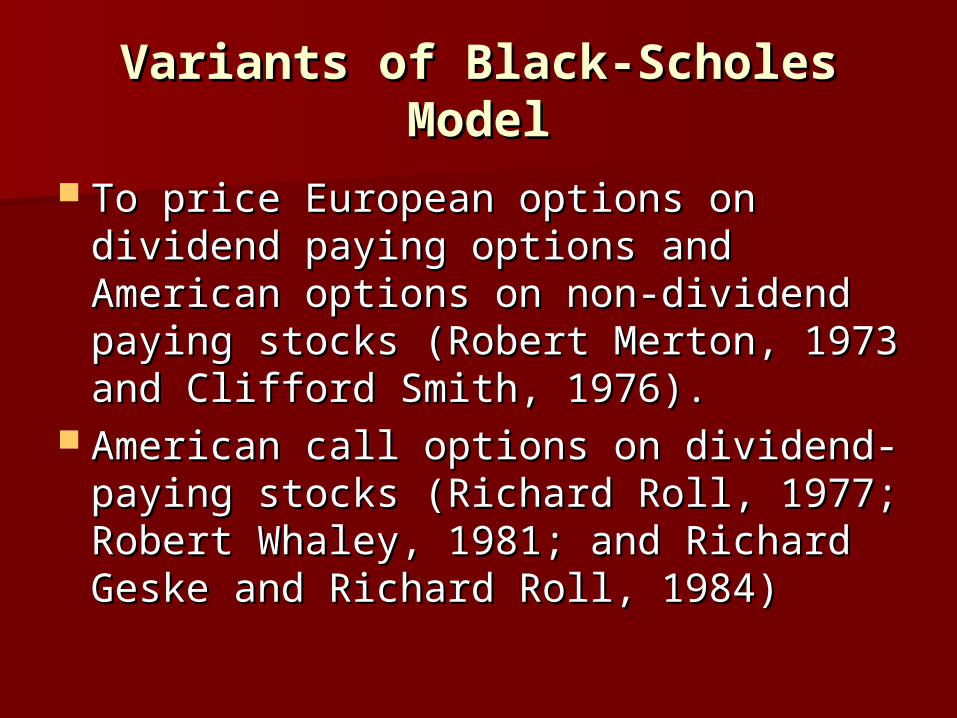
Variants of Black-Scholes Variants of Black-Scholes ModelModel
To price European options on To price European options on dividend paying options and dividend paying options and American options on non-dividend American options on non-dividend paying stocks (Robert Merton, 1973 paying stocks (Robert Merton, 1973 and Clifford Smith, 1976).and Clifford Smith, 1976).
American call options on dividend-American call options on dividend-paying stocks (Richard Roll, 1977; paying stocks (Richard Roll, 1977; Robert Whaley, 1981; and Richard Robert Whaley, 1981; and Richard Geske and Richard Roll, 1984)Geske and Richard Roll, 1984)

Variants of Black-Scholes Variants of Black-Scholes ModelModel
When price changes are When price changes are discontinuous (Cox, Rubinstein and discontinuous (Cox, Rubinstein and Ross, 1979). This was published in Ross, 1979). This was published in Journal of Financial Economics as Journal of Financial Economics as “Option Pricing: A Simplified “Option Pricing: A Simplified Approach”. This is the Binomial Approach”. This is the Binomial Model for Option Pricing.Model for Option Pricing.

Garman - Kohlhagen ModelGarman - Kohlhagen Model
The foreign currency option pricing The foreign currency option pricing model is equivalent to the Black-model is equivalent to the Black-Scholes mode except that the spot Scholes mode except that the spot rate is discounted by the foreign rate is discounted by the foreign interest rate and appears instead of interest rate and appears instead of the Stock Price.the Stock Price.

Sensitivity of Option PremiumsSensitivity of Option Premiums
An option’s intrinsic value is the amount An option’s intrinsic value is the amount by which it is in the money and the time by which it is in the money and the time value is the difference between actual value is the difference between actual premium and the intrinsic value i.e. premium and the intrinsic value i.e. premium = intrinsic value + time value.premium = intrinsic value + time value.
At the money option has highest At the money option has highest likelihood of gaining intrinsic value as likelihood of gaining intrinsic value as compared to that of losing. It has no compared to that of losing. It has no value to lose but 50-50 chance of value to lose but 50-50 chance of gaining.gaining.

Sensitivity of Option PremiumsSensitivity of Option Premiums
Delta (Delta (δδ):): Change in option price Change in option price relative to the price of underlying relative to the price of underlying asset. Reverse of Delta is used to asset. Reverse of Delta is used to calculate a hedge ratio.calculate a hedge ratio.
Gamma:Gamma: The rate of change of Delta. It The rate of change of Delta. It is the second derivative of option price is the second derivative of option price with respect to price of the asset and is with respect to price of the asset and is also known as option’s curvature. High also known as option’s curvature. High gamma makes option less attractive.gamma makes option less attractive.

Sensitivity of Option PremiumsSensitivity of Option Premiums
Lambda:Lambda: Change in option price relative Change in option price relative to change in volatility. Its value lies to change in volatility. Its value lies between zero and infinity and declines between zero and infinity and declines as option approaches maturityas option approaches maturity
Theta:Theta: Change in option price relative to Change in option price relative to Time to Expiration. The value of theta Time to Expiration. The value of theta lies between zero and total value of lies between zero and total value of option.option.
Rho:Rho: Change in option value in relation to Change in option value in relation to interest rates and varies from type to interest rates and varies from type to type of the options.type of the options.

Sensitivity of Option PremiumsSensitivity of Option Premiums
Implied volatility is obtained by finding Implied volatility is obtained by finding the S.D. that when used in the Black-the S.D. that when used in the Black-Scholes model makes the model price Scholes model makes the model price equal to market price of the option.equal to market price of the option.
The pattern of implied volatility across The pattern of implied volatility across expirations is often called the term expirations is often called the term structure of volatility, and the pattern structure of volatility, and the pattern of volatility across exercise prices is of volatility across exercise prices is often called the volatility smile or often called the volatility smile or skew.skew.
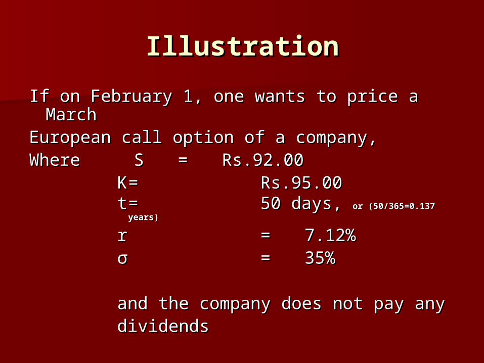
IllustrationIllustration
If on February 1, one wants to price a MarchIf on February 1, one wants to price a MarchEuropean call option of a company,European call option of a company,Where Where SS == Rs.92.00Rs.92.00
KK = = Rs.95.00Rs.95.00tt == 50 days, 50 days, or or
(50/365=0.137 years)(50/365=0.137 years)
r r = = 7.12%7.12%σσ == 35%35%
and the company does not pay anyand the company does not pay anydividendsdividends

Return RelativesReturn Relatives
If P(0) is the beginning wealth and If P(0) is the beginning wealth and P(T), the ending wealth, the price P(T), the ending wealth, the price relative R(0,T) is given by P(T)/P(0). relative R(0,T) is given by P(T)/P(0). Since P(T) is a random variable, Since P(T) is a random variable, P(T)/P(0) is also a random variable.P(T)/P(0) is also a random variable.
Holding period return is the Holding period return is the effective return r(T) is related to effective return r(T) is related to R(0,T).R(0,T).
Continuous holding period return Continuous holding period return rrcc(T) is related to price relative by: (T) is related to price relative by: rrcc(T) = ln(R(0,T)).(T) = ln(R(0,T)).
Thus all these are random variables.Thus all these are random variables.