Embed Size (px)
Citation preview

The author(s) shown below used Federal funds provided by the U.S.Department of Justice and prepared the following final report:
Document Title: Gang Activity in Orange County, California:Final Report to the National Institute of Justice
Author(s): Bryan J. Vila Ph.D., James W. Meeker Ph.D.
Document No.: 181242
Date Received: February 2000
Award Number: 96-IJ-CX-0030, 96-CN-WX-0019
This report has not been published by the U.S. Department of Justice.To provide better customer service, NCJRS has made this Federally-funded grant final report available electronically in addition totraditional paper copies.
Opinions or points of view expressed are thoseof the author(s) and do not necessarily reflect
the official position or policies of the U.S.Department of Justice.

Gang Activity in Orange County, California
GANG ACTIVITY IN ORANGE COUNTY, CALIFORNIA
Final Report to the National Institute of Justice
Award Number: 96-IJ-CX-0030
Principal Investigators:
Bryan J. Vila, Ph.D.
University of Wyoming
James W. Meeker, J.D., Ph.D.
University of California, Irvine
August 1999 The authors would like to thank the invaluable assistance of the research assistants on this project: Thomas E. Fossati, Ph.D., Jodi Lane, Ph.D., Katie J.B. Parsons, Ph.D., and Douglas Wiebe. We would also like to thank Darcy Purvis for her editorial help. This research would not have been possible without the cooperation of the Orange County Police Chiefs and Sheriff's Association Steering Committee on Juvenile Justice and Gangs and its Chair James Cook, Police Chief of Westminster. This report was prepared under grant number 96-IJ-CX-0030 from the National Institute of Justice, U.S. Department of Justice. The public survey of fear was also partially supported by grant number 96-CN-WX-0019 from the Office of Community Oriented Policing Services, U.S. Department of Justice. We would also like to thank the helpful comments of anonymous reviewers of earlier drafts of this report. Points of view or opinions expressed in this document are those of the authors and do not necessarily represent the official position or policies of the National Institute of Justice or the U. S. Department of Justice.

Gang Activity in Orange County, California a
TABLE OF CONTENTS
Executive Summary vi
Introduction
Organization of Report 1
Project Overview 2
Project History 3
Data Collection 6
Research Objectives 8
Dissemination of Project Information 11
Objective 1: Understanding Gang Crime and Anti-Gang Strategies
Nature and Distribution of Gang Incidents, 1994–1997 12
Findings for 1994–1997 Gang-Related Crimes 13
Temporal Distribution of Gang Incidents: Hourly Trends for Juvenile and Adult
Arrest Incidents, 1994–1996 21
Explaining Violent Gang Crime Variation 28
Using GITS to Evaluate the Effectiveness of Anti-Gang Strategies 53
Objective 2: Fear of Gang Crime
Literature Review 61
Fear of Crime and Gangs Survey Methods 66
Analysis of Random Digit Dial Survey Findings 70
Impact of Fear of Gang Crime 92
Comparing Perceptions of Gang Crime with Reported Levels 94
Ethnicity as a Predictor of Perceived Seriousness, Risk, and Fear of Gang Crime 97
Conclusions 104
Final Report - Aug 99 i

Gang Activity in Orange County, California
Objective 3: GITS Validity and Reliability Evaluation
Validity of Gang Incident Measures 107
Observations Regarding Use of Definitional Criteria 112
Validation of Data Collected 117
Data Coding Reliability Tests 119
Improving GITS Data Collection 120
Objective 4: GITS Program Evaluation
Findings 125
Goal Analysis 128
GITS Benefits, Expected and Unexpected 132
Structure of Interagency Cooperation 133
Summary
Discussion of Findings 136
Future Research Opportunities 139
References 141
Appendix A: GITS Data Coding Forms 153
Appendix B: Fear of Crime and Gangs Survey 160
Appendix C: Dissemination of Project Information Activities 174
List of Figures
Figure 1. Information flow into the GITS database 7
Figure 2. Percentage of incidents in each major crime category 16
Figure 3. Adult and juvenile arrests in gang-related incidents 17
Figure 4. Known motivating factors in Orange County gang incidents, 1994-1997 18
Figure 5. Known victims of gang incidents, 1994-1997 19
Figure 6. Known victims of violent gang incidents, 1994-1997 20
Figure 7. Firearm use in gang-related incidents 21
Final Report – Aug 99 ii

Gang Activity in Orange County, California
Figure 8. Hourly number of juvenile gang-related arrest incidents on 550 schooldays
(n=1,155) and 546 non-schooldays (n=838) in 1994–1996 22
Figure 9. Hourly number of adult gang-related arrest incidents on 550 schooldays
(n=1,034) and 546 non-schooldays (n=1,180) in 1994–1996 24
Figure 10. Hourly number of juvenile gang-related violent (n=605), property (n=413)
and tagging (n=374) arrest incidents in 1994–1996 26
Figure 11. Hourly number of adult gang-related violent (n=854), property (n=363) and
tagging (n=145) arrest incidents in 1994–1996 27
Figure 12. Violent gang incidents by census tract. 33
Figure 13. Predicted values for violent gang incidents based on OLS regression 41
Figure 14. Moran scatterplot of OLS residuals with regression line 43
Figure 15. OLS residuals by Moran Quadrant 44
Figure 16. Significantly large positive and negative standardized residuals 45
Figure 17. SAR model predicted values for Orange County census tracts 48
Figure 18. Moran scatterplot of SAR residuals with regression line 49
Figure 19. SAR residuals by Moran Quadrant 50
Figure 20. Significantly large residuals for the SAR regression model 51
Figure 21. Location of incidents committed by gang A in 1994 57
Figure 22. Location of incidents committed by gang A in 1995 58
Figure 23. Location of incidents committed by gang A in 1996 59
Figure 24. Structural equation model predicting fear of crime and gangs 91
Figure 25. Percentage of reported gang-related incidents by judicial district 96
Figure 26. Gang incident hot spots for Orange County judicial districts 96
Figure A1. Original GITS Coding Form 154
Figure A2. Revised GITS Coding Form 158
Figure A3. Revised GITS Coding Form Instructions 159
Final Report – Aug 99 iii

Gang Activity in Orange County, California
List of Tables
Table 1. Major crime categories 14
Table 2. Detailed crime incidents by year 15
Table 3. Descriptive statistics for violent incident measures in Orange County census
tracts 32
Table 4. Description of data sources used and variable information for community
structure 34
Table 5. Descriptive statistics for census measure of community structure 35
Table 6. Principal components eigenvalues for community structure dimensions 36
Table 7. Principal components loadings: varimax rotated solution 36
Table 8. Reliability results for items used in creation of community dimensions 38
Table 9. Descriptive statistics for OLS regression model 39
Table 10. Results from OLS regression model 40
Table 11. Results from SAR regression model 46
Table 12. Theoretical constructs and survey questions used to measure them 69
Table 13. RDD respondents rank the seriousness of eight crimes 71
Table 14. RDD respondents indicate the likelihood that they will become a victim of
eight crimes in the next 2-3 years 72
Table 15. RDD respondents indicate how personally afraid they are of eight crimes 73
Table 16. Predicting crime seriousness based upon RDD respondent demographic
characteristics 76
Table 17. Predicting perceived risk of victimization based upon RDD respondent
demographic characteristics 77
Table 18. Predicting personal fear based upon RDD respondent demographic
characteristics 78
Table 19. Predicted perceptions of seriousness based upon demographic, disorder, and
diversity variables 82
Table 20. Predicted perceived risk of victimization based upon demographic, disorder,
and diversity variables 83
Table 21. Predicting personal fear based upon demographic, disorder, and diversity
variables 84
Final Report – Aug 99 iv

Gang Activity in Orange County, California
Table 22. Predicting fear of crime from demographics, perceived seriousness and
perceived risk 88
Table 23. Predicting fear of crime from demographics, community concerns, perceived
seriousness, and perceived risk 89
Table 24. Perceptions of current community crime levels and crime changes in the last
two to three years 93
Table 25. Gang crime avoidance behaviors 94
Table 26. Tukey HSD comparisons of ethnic differences in seriousness ratings for eight
crimes 98
Table 27. Tukey HSD comparisons of ethnic differences in perceived risk of
victimization for eight crimes 99
Table 28. Tukey HSD comparisons of ethnic differences in fear for eight crimes 100
Table 29. Predicting seriousness ratings of eight crimes based upon ethnicity and region
of residence 101
Table 30. Predicting perceived risk of victimization of eight crimes based upon ethnicity
and county region of residence 102
Table 31. Predicting fear of eight crimes based upon ethnicity and county region of
residence 103
Final Report – Aug 99 v

Gang Activity in Orange County, California
EXECUTIVE SUMMARY: GANG ACTIVITY IN ORANGE COUNTY
Background
This analysis of “Gang Activity in Orange County” began in March 1995, when the
Orange County Chiefs’ and Sheriff’s Association (OCCSA) asked the University of California,
Irvine (UCI) to enter into a long-term partnership to assist them in evaluating and monitoring the
effectiveness of their community-based, multi-agency efforts to address gang violence.
In response, the UCI School of Social Ecology established a Focused Research Group
(FRG) on Gangs within its Department of Criminology, Law & Society. The goal of the FRG
was to work with OCCSA and its countywide Gang Strategy Steering Committee (GSSC) to
resolve a number of previously intractable questions about gangs, gang crime, and their effects
on the community, and help them develop strategies to prevent and control illegal gang activity.
Co-principal investigators for the UCI FRG were Dr. Bryan J. Vila (now with the
University of Wyoming) and Dr. James W. Meeker. Drs. Vila and Meeker supervised the work
of four UCI doctoral students: Thomas E. Fossati, Ph.D.; Jodi Lane, Ph.D.; Katie J.B. Parsons,
Ph.D.; and Douglas Wiebe, ABD.
Initial funding for the project was provided by $30,000 seed-money grants from Pacific
Mutual Corp. of Newport Beach, California, and UCI. Two-year funding for the study reported
here was received from the U.S. Department of Justice’s National Institute of Justice (Award
Number 96-IJ-CX-0030) in 1996. Additional support for technical assistance to participating
law enforcement agencies was received as part of a grant to OCCSA from the Office of
Community Oriented Policing Services (PNG-22294),
Final Report – Aug 99 vi

Gang Activity in Orange County, California
One of the primary programs developed by OCCSA and GSSC to be evaluated during the
two-year study was the Orange County Gang Incident Tracking System (GITS). GITS was
established in 1993 to document the extent of gang-related crime in the county and provide
information for strategic planning and evaluation purposes by establishing a baseline against
which to identify future trends in gang-related crime over time, and determining regional
variation in gang-related crime patterns.
GOALS
GITS collected more, and more detailed, cross-jurisdictional information about gang
incidents than had ever been assembled before. So long as these data provide a reasonably valid,
reliable, and complete picture of gang activity, they pose a unique opportunity to evaluate the
nature, extent, and effects of street gang crime in a large metropolitan region. Therefore, our
main research objectives were to:
• Evaluate the validity and reliability of GITS data;
• Describe and, if possible, explain the nature and distribution of gang crime using
geographic information systems and multi-variate statistical techniques as well as attempt
to assess the effectiveness of various gang prevention, intervention, and control strategies;
• Determine the effects of fear of gangs and gang crime on residents of Orange County; and
• Evaluate how well GITS met the initial goals set for it.
Following is a brief summary of some of the more important findings from this study:
Key Findings
VALIDITY
• Data being collected by GITS appears to present a reasonably unbiased and complete
picture of gang incidents handled by the police. The study found little evidence to support
Final Report – Aug 99 vii

Gang Activity in Orange County, California
concerns that the police are drastically over-estimating gang-related crime in Orange
County. In fact, based on a substantial number of ride-alongs and interviews, as well as
field observation, and evaluation of official records, we found that law enforcement
agencies tend to under-report gang incidents to the GITS database.
• Orange County’s concentrated effort to train officers about legal criteria in California for
defining who is a gang member appears to have paid off. Contrary to some claims, we
found no evidence that officers were classifying young people as gang members merely
because of their mode of dress, ethnicity, or place of residence when they reported gang
incidents for use in the countywide database.
NATURE AND DISTRIBUTION OF GANG INCIDENTS
• There were 3,600 gang-related incidents reported to the GITS database in 1994, 3,407 in
1995, 3,408 in 1996, and 3,227 in 1997. Of these incidents, the majority of gang-related
crimes committed each year were violent crimes—45.2 percent, 46.9 percent, 53.8
percent, and 48.9 percent, respectively. Vandalism/graffiti was the next most frequent
gang-related crime during this four-year period (23.4 percent, 21.3 percent, 21 percent,
and 31.6 percent, respectively), followed by weapons violations (15.1 percent, 16.1
percent, 15.3 percent, and 11.7 percent, respectively) and property crimes (13.7 percent,
12.5 percent, 6.9 percent and 6.3 percent, respectively), and narcotic sales (2.6 percent,
3.3 percent, 3.0 percent, and 1.5 percent, respectively).
• Overall, adult street gang crime in Orange County appears to be a more serious problem
than juvenile gang crime. While similar proportions of juveniles and adults were arrested
for gang-related incidents reported to the police, adults have much higher violent arrest
rates than juveniles, and—compared to juveniles—a much lower proportion of gang-
related adult arrests are for property crimes.
• The data clearly suggest that adult and juvenile gang intervention strategies reflect
different needs at different times of the day. Adult offenses for all types of crime are
unaffected by schoolday and non-schoolday periods; that is, they show similar time-of-
day patterns during either period. In contrast, gang-related juvenile offenses peak much
earlier in the day on schooldays. Moreover, the number of juvenile gang-related arrests at
Final Report – Aug 99 viii

Gang Activity in Orange County, California
the peak hours on schooldays (from 2–2:59 p.m.) is much higher than at the peak on non-
schooldays (from 11–11:59 p.m.). Another important difference between juvenile and
adult gang-related arrests is that, on schooldays, the number of juvenile arrests for all
offenses increases sharply early in the day (climbing steadily from 7 a.m. to 3:59 p.m.),
whereas adult arrests climb slowly throughout the day and peak in the evening.
• Regional approaches such as the one mounted by the Orange County Chiefs’ and
Sheriff’s Association are required for tracking, understanding, or addressing street gang
problems. We found that communities tend to be significantly impacted by violent crime
in neighboring communities. This means that any attempt to reduce the gang problem in
areas of Orange County where it is more concentrated will have to consider neighboring
communities as well.
FEAR OF GANGS AND GANG CRIME
The focus of the study is on gang crime and associated fears. We specifically studied
perceptions of fear, risk, and seriousness for six crimes typically association with gangs and two
crimes that are not.
• Overall, women tend to be more afraid than men of all eight crimes measured in the
study—graffiti, home invasion robbery, drive-by shootings, physical assault, harassment,
carjacking, burglary, and rape. However, women’s perceived risk of actually being a
victim of these crimes was significantly related only to burglary and rape. Therefore,
although women report more fear of all eight crimes than do men, they don’t necessarily
feel more at risk. Women also are more likely to rate crimes, except carjacking, as more
serious than do men.
• Age was found to be negatively related to ratings of seriousness for gang-related assault,
carjacking, and home invasion robbery—i.e., younger residents tended to rate these crimes
as more serious than did older residents. Younger residents also perceived greater risk of
graffiti, gang-related harassment, and gang-related assault than did older residents, and
were more fearful of gang-related assault, carjacking, home invasion robbery, drive-by
shootings, and rape.
Final Report – Aug 99 ix

Gang Activity in Orange County, California
• Although lower income and education were significantly related to perceived risk for most
of the crimes in the study, income was not significantly related to fear of any of the
crimes.
• Prior victimization was related to perceived risk of future victimization, but not
significantly related to fear of any of the crimes.
• Whites generally were more likely to rate the crimes named in the study as serious. But in
terms of risk and fear, Vietnamese felt more at risk and more fearful than Hispanics, who
felt significantly more at risk and more fearful than whites.
• As with previous studies, concern about community disorder was a significant predictor of
perceived risk and fear for almost all of the crimes. However, concern about community
diversity was not significantly related to seriousness ratings, perceived risk, or fear of any
of the crimes named in the study.
Final Comments
The Gang Incident Tracking System (GITS) project clearly demonstrates the
usefulness—and the necessity—of multi-jurisdictional efforts to understand, prevent, intervene
with, and suppress street gang activities. Just as clearly, we think, it demonstrates the value of
partnerships between criminal justice practitioners and university researchers.
One of the most heartening surprises associated with this project is that several dozen law
enforcement and community agencies can collaborate successfully with one another and with a
team of university researchers. The Orange County Chief’s and Sheriff’s Association and the
county Gang Strategy Steering Committee provide an excellent model for regions struggling
with the reality that crime often is multi-jurisdictional in nature. The findings reported here
provide evidence of the utility of this type of cooperative endeavor for practitioners. They also
reveal opportunities for fruitful scholarly research (see Summary and Conclusions).
Final Report – Aug 99 x

Gang Activity in Orange County, California
INTRODUCTION
Organization of Report
This is the final report for a research grant titled “Gang Activity in Orange County”
awarded to the University of California, Irvine (UCI) by the U.S. Department of Justice’s
National Institute of Justice (Award Number 96-IJ-CX-0030). The grant was administered by
the UCI School of Social Ecology. Co-principal investigators were Dr. Bryan J. Vila (now with
the University of Wyoming) and Dr. James W. Meeker.
Drs. Vila and Meeker supervised the work of four UCI doctoral students, each of whom
took the lead on a different aspect of the project; developing the research design, overseeing
implementation, conducting analyses, and preparing draft reports. Three of the students, Thomas
E. Fossati, Ph.D.; Jodi Lane, Ph.D.; and Katie Parsons, Ph.D., worked on the project from its
inception in March 1995. Douglas Wiebe, ABD, joined the project in 1997. Although Drs. Vila
and Meeker bear sole responsibility for the work reported here, we acknowledge the invaluable
role played by Fossati, Lane, Parsons, and Wiebe. Although their individual contributions are
noted as appropriate in each of the following sections of the report, it is important to recognize
that during the course of the project each student participated in a wide variety of activities. We
also gratefully acknowledge the diligent work of more than 20 undergraduate research assistants
who entered data, checked the accuracy of locator data, and assisted with database development.
The report first provides an overview of the GITS project and relevant history regarding
its development. After a collective description of the project’s research goals, each of the goals
is treated as a separate chapter that discusses key problems, describes research methods and
analysis, then presents findings. Because one of the non-research goals of this project was the
Final Report – Aug 99 1

Gang Activity in Orange County, California
dissemination of information to scholars, practitioners, and relevant officials, we next list
scholarly publications that have been made or are currently being prepared, conference
presentations, public presentations, and reports prepared by project staff for local government
agencies. The report ends with a summary discussion of findings and future research needs.
Project Overview
In recent years, many communities that previously considered themselves insulated from
inner-city problems have been forced to acknowledge that gang violence also can extend into
their neighborhoods (Curry, Ball and Fox, 1994; Spergel and Curry, 1995). Orange County,
California is one such community. Located 40 miles south of Los Angeles, Orange County is a
highly heterogeneous suburban county with 2.7 million people living in 31 cities and
unincorporated areas. Since 1980, the county has experienced rapid growth, increasing
urbanization, and racial and ethnic change. Despite a few traditional Hispanic “turf” gangs
firmly entrenched in its less affluent areas (see Vigil and Long, 1990), Orange County
historically has enjoyed low crime rates and relative tranquility.
During the past decade, however, gang activity appears to have been on the rise in the
county. In 1991, the Orange County Grand Jury reported that gang problems were escalating at
an alarming rate, a sentiment echoed by the 1995 Orange County Grand Jury. According to
police and media reports, gang crime in Orange County not only had become more frequent, but
more violent. More mobile Asian gangs, as well as white “skinhead” gangs have emerged within
the county, along with a growing number of more traditional turf-oriented gangs.
Final Report – Aug 99 2

Gang Activity in Orange County, California
Orange County residents also have become increasingly concerned about gangs and
crime. A 1994 survey1 found that 75 percent of residents were aware of gang problems in their
community, and 61 percent thought gang activities have increased in the past few years. In
addition, the Orange County Annual Survey2 found that residents' worries about crime—once a
low concern—ranked highest on the list of county problems for the first time in 1993 and again
in 1994.
Project History
In response to escalating gang activities that often overlapped jurisdictional boundaries,
the Orange County Chiefs' and Sheriff's Association (OCCSA) established a countywide Gang
Strategy Steering Committee (GSSC) in 1992. Joining forces with school districts, local
government agencies, community groups, and businesses, all 22 law enforcement agencies in the
county developed and implemented an unprecedented community-based, multi-agency effort to
address gang violence.
Since then, following the recommendations of the California State Task Force on Gangs
(1989:37, 57), OCCSA launched a comprehensive set of programs:
• Project No Gangs, a countywide community education and awareness prevention program
aimed at mobilizing community resources to fight the influence of gangs;
• TARGET, a suppression program strategically located in eight cities involving law
enforcement, probation, and prosecution staff in targeting hard-core gang leaders and
repeat offenders through vigorous surveillance and prosecution (Kent and Smith, 1995);
1 The survey, conducted for Drug Abuse is Life Abuse, involved random telephone interviews with 600 adult Orange County residents (Mark Baldassare and Associates, 1994). 2 A random telephone survey of 1,000 adult county residents conducted annually since 1982 (Baldassare and Katz).
Final Report – Aug 99 3

Gang Activity in Orange County, California
• The Gang Incident Tracking System (GITS), designed to document the extent of gang-
related crime in the county and provide information for strategic planning and evaluation
purposes (Vila and Meeker, 1997).
Although OCCSA laid the foundation for interagency coordination and data collection, it
lacked the analytical resources and expertise to fully evaluate and monitor the effectiveness of
these programs. Early in 1995, OCCSA asked UCI to enter into a long-term partnership to
enhance their analytical capabilities. The UCI School of Social Ecology established a Focused
Research Group (FRG) on Gangs within its Department of Criminology, Law & Society. In
keeping with the School’s tradition for using innovative research techniques to tackle important
community problems in a holistic fashion, the goal of the FRG was to work with OCCSA and
GSSC to resolve a number of previously intractable questions about gangs, gang crime, and their
effects on the community and help them develop strategies to prevent and control illegal gang
activity.
GITS
Orange County's Gang Incident tracking System (GITS) is intended to accurately
identify the extent of gang-related crime in Orange County, establish a baseline against which to
identify future trends in gang-related crime over time, and determine regional variation in gang-
related crime patterns. This information is used by Orange County law enforcement agencies to
facilitate strategic planning and improve resource allocation for controlling gang activities.
GITS became operative January 1, 1993, when county law enforcement agencies began
reporting all gang-related incidents, based on police reports, to a centralized database. By the
end of 1993, all 22 independent cities and the Orange County Sheriff-Coroner's Department
(which serves contract cities and unincorporated areas) had established relatively consistent
internal procedures for identifying and tracking gang-related crime, and were reporting to the
Final Report – Aug 99 4

Gang Activity in Orange County, California
centralized database. Training programs and a short training videotape were used to teach patrol
officers countywide how to identify and report gang-related incidents to GITS. The GSSC
declared publicly that 1994 GITS data was to be the benchmark by which future law
enforcement activities involving gang activities would be judged.
To help avoid discrepancies between agencies, the GSSC definition of the term “gang”
closely follows the one used in California's Street Terrorism Enforcement and Prevention
(STEP) Act (CPC §186.22), “…a group of three or more persons who have a common
identifying sign, symbol or name, and whose members individually or collectively engage in or
have engaged in a pattern of criminal activity creating an atmosphere of fear and intimidation in
the community.”
Gang-related crimes were defined as those where:
• Suspects(s) are identified as gang members, or admit(s) membership in a gang;
• A person becomes a victim due to his/her gang association;
• A reliable informant identifies an incident as gang activity; or
• An informant of previously untested reliability identifies an incident as gang activity, and
it is corroborated by other independent information.
Incidents also may be included that do not fit these criteria if there are strong indications
of gang involvement (e.g., suspects display gang hand signs, or the incident fits the profile of
gang incidents, such as drive-by shootings, or home invasion robberies).
The definition adopts the gang-involved definition of gang crime. This is often called the
Los Angeles model because of its adoption by law enforcement in that county. The other
definition used by law enforcement is the gang-motivated, or Chicago model. This definition
restricts gang crime to incidents that have a clear gang motivation. The gang-involved model is
the broader perspective including not only gang-motivated crime, but all crime involving gang
Final Report – Aug 99 5

Gang Activity in Orange County, California
members. While the gang-involved definition will clearly include more crime, the limited
research on this issue to date suggests both definitions cover crimes that produce similar patterns
in factors associated with the crime (see Maxson and Klein, 1990 and 1996).
Data Collection
GITS DATABASE DEVELOPMENT
The original GITS reporting forms (Appendix A) collected information on gang
identification, map grid location, 21 crime categories, and number of juveniles and adults
arrested during each incident. Additional information about motivating factors, drugs and
alcohol, and weapons involved in the incident also were collected, as was information about
victim/offender relationship. The form was changed in 1995 to collect specific address data, and
all 1994 cases were updated to include address. For reporting purposes, the type of incident is
divided into three primary categories: violent crime, property crime, and other crime.
In 1996 the data coding forms were revised based upon input from all jurisdictions
(Appendix B). There were two major category changes. First, the crime categories were
expanded to allow coders to list the penal code violations associated with each incident on the
departmental reports. This eliminated the need for coders to translate specific penal codes into
the 1994–1995 crime categories, reducing error. Coders also were given the opportunity to
indicate more than the most serious crime related to the incident; this provided an opportunity to
identify most of the crimes associated with each incident. Another major change in the data
coding form was the inclusion of a victim relationship category. On the 1994–1995 forms, the
victim category was not reliable due to overlapping meanings in the categories. This created
confusion for coders and resulted in unreliable coding. The new form was modified to clear up
Final Report – Aug 99 6
Gang Activity in Orange County, California
confusion and to reflect the desire for information about gang-on-gang crime versus gang-on-
non-gang crime.
THE REPORTING PROCESS
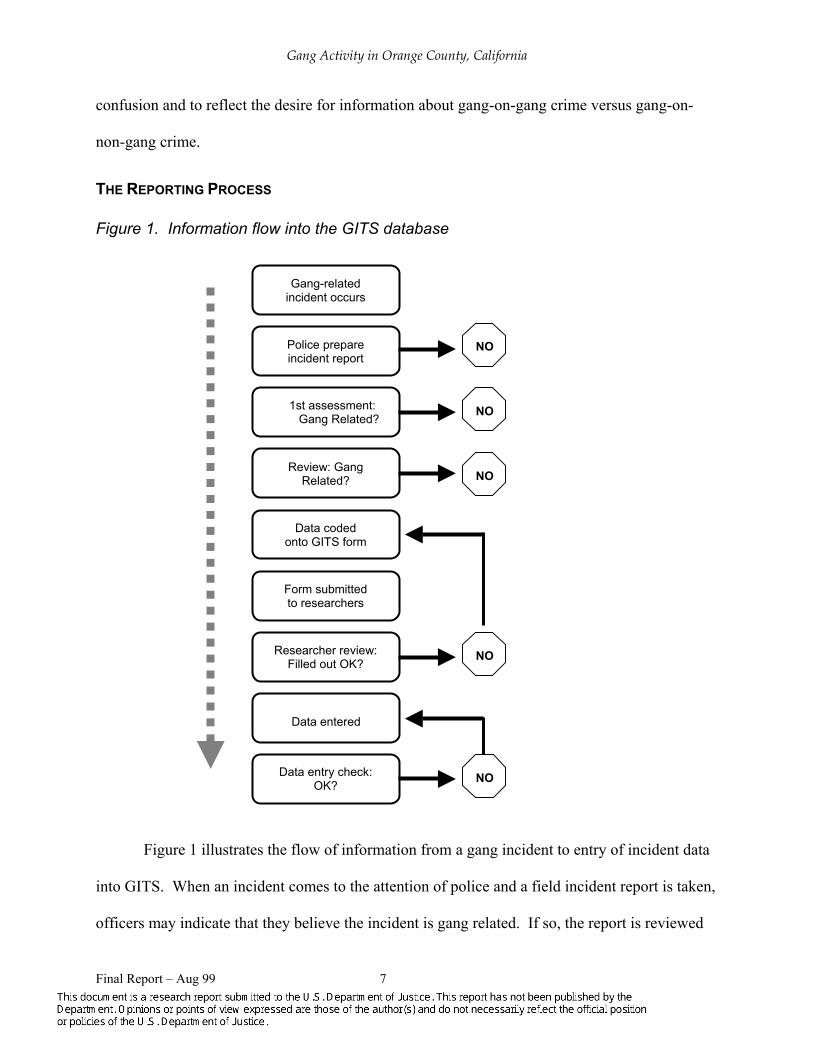
Figure 1. Information flow into the GITS database
Data coded onto GITS form
Form submitted to researchers
Data entered
1st assessment: Gang Related?
Review: Gang Related?
Researcher review:Filled out OK?
Data entry check: OK?
Gang-related incident occurs
NO
NO
NO
NO
NO
Police prepare incident report
Figure 1 illustrates the flow of information from a gang incident to entry of incident data
into GITS. When an incident comes to the attention of police and a field incident report is taken,
officers may indicate that they believe the incident is gang related. If so, the report is reviewed
Final Report – Aug 99 7

Gang Activity in Orange County, California
later by the person responsible for review of departmental reports for possible inclusion in GITS.
If the review process is working properly (see reliability evaluation later on), every field incident
report also receives another review for gang-relatedness. Gang-related incidents then are coded
onto the GITS form by individuals assigned that task in each department and forwarded to the
research team. There, the forms are reviewed for completeness and potential errors. Those that
fail this screening are rejected and returned to the department for correction. Those that pass are
entered into the GITS database. Once data have been entered, a member of the project team
conducts a last check to assure that they were entered accurately. If not, the errors are corrected.
Research Objectives
The Orange County Gang Incident Tracking System (GITS) collected more, and more
detailed, cross-jurisdictional information about gang incidents than had ever been assembled
before. So long as these data provide a reasonably valid, reliable, and complete picture of gang
activity, they pose a unique opportunity to evaluate the nature, extent, and effects of street gang
crime in a large metropolitan region. Our initial research objectives were to:
• Evaluate the validity and reliability of GITS data;
• Describe and, if possible, explain the nature and distribution of gang crime as well as
attempt to assess the effectiveness of various gang prevention, intervention, and control
strategies;
• Determine the effects of fear of gangs and gang crime on residents of Orange County; and
• Evaluate how well GITS met the initial goals set for it.
Obviously, it would not be possible to exhaust the research potential of such an extensive data
collection project—especially when more than half of project staff time was devoted to mundane
tasks such as data collection, entry, and geocoding as well as the endless coordination and
Final Report – Aug 99 8

Gang Activity in Orange County, California
administrative tasks associated with the cooperative effort of more than 30 government agencies.
In the following four sections we present results of our evaluation of GITS reliability and
validity and our assessment of the effects of fear of gangs and gang crime on county residents.
We also describe the nature and extent of gang crime in the region and present results of
explanatory research (with the caveat that there still is substantial potential in the data with
regard to explaining gang crime).
Objective 1: Understanding Gang Crime and Anti-Gang Strategies. Use geographic
information system and multi-variate statistical techniques to analyze the extensive Orange
County gang incident data collected by OCCSA in order to (1) increase understanding of the
nature and distribution of gang incidents reported by the police, and (2) test the effectiveness of
different gang prevention and control efforts initiated by law enforcement agencies, such as
“street sweeps” and targeting gang leadership. Potential research questions under this objective
included:
• What is the extent of the gang problem in Orange County?
• How many gang-related incidents are there?
• How many gangs are there, where are they located, how many members do they have,
what are their personal characteristics, and what types of crimes do they commit?
• Are there statistically significant relationships between gang incidents reported by police
in Orange County and social, economic, demographic, educational, ecological and
geographical variables?
• What strategies are likely to be more effective for combating gang crime?
• Are different control and prevention strategies effective against different types of gangs?
• Does suppression of gang activities in one area displace them to another area?
Final Report – Aug 99 9

Gang Activity in Orange County, California
• Does suppression of one type of gang activity deflect gang members toward other types of
crime?
• What effect does removal of gang leaders have (i.e., does it lead to more or less violence
by gang members and is any increase in violence focused inside or outside the gang)?
Objective 2: Fear of Gang Crime. Identify factors that contribute to community
members’ perceptions of—and fears about—gang violence and compare residents’ fears to
actual levels of gang activity in the county so that law enforcement efforts may be targeted to
address community concerns more efficiently and effectively. Potential research questions under
this objective included:
• How much fear do Orange County residents currently have about gang violence?
• How closely are these fears related to actual risks of victimization?
• What factors have the most impact on residents’ perceptions of, and fears about, gang
activity?
• What effect does increased gang violence—or the perception of increased gang
violence—have on residents’ day-to-day activities and quality of life?
Objective 3: GITS Validity and Reliability Evaluation. Determine how completely,
accurately and reliably Orange County law enforcement agencies measure illegal gang activity.
Potential research questions under this objective included:
• Are current techniques for measuring gang-related incidents and violence and for
identifying gang members valid?
• How consistently are gang members and gang-related incidents identified by officers
within and between law enforcement agencies?
Final Report – Aug 99 10

Gang Activity in Orange County, California
• What can be done to improve collection of data on gangs and gang incidents in Orange
County?
Objective 4: GITS Program Evaluation. Determine how well GITS meets the goals
originally set by law enforcement officials and identify ways to improve the original program
goals.
Dissemination of Project Information
Another of the project deliverables was an active effort to disseminate information to
academics, practitioners, and policy makers. Since 1995, we have presented 23 conference
papers on GITS research, given 17 talks to practitioner bodies and the general public, prepared
nine extensive reports for local agencies, and prepared two more specialized analyses for federal
agencies. We also have published three doctoral dissertations, one refereed journal article—with
an additional eight under preparation along with a book. Appendix C provides a complete listing
of publications, presentations, and other information dissemination activities.
Final Report – Aug 99 11

Gang Activity in Orange County, California
OBJECTIVE 1: UNDERSTANDING GANG CRIME AND ANTI-GANG
STRATEGIES
Our objective in this portion of the research was to analyze the extensive Orange County
gang incident data collected by OCCSA using geographic information system software and
multivariate statistical analysis techniques to (1) increase understanding of the nature and
distribution of gang incidents reported by the police, and (2) test the effectiveness of different
gang prevention and control efforts initiated by law enforcement agencies, such as “street
sweeps” and targeting gang leadership. Dr. Katie J.B. Parsons shouldered primary responsibility
for oversight of data screening and entry activities, Dr. Thomas E. Fossati was team leader for
crime mapping and geospatial analyses. Mr. Douglas Wiebe took a leadership role with regard
to temporal analyses and the evaluation of gang prevention and control efforts.
Nature and Distribution of Gang Incidents, 1994-1997
GANG INCIDENT TRACKING SYSTEM DATABASE
The original Gang Incident Tracking System (GITS) reporting forms collected
information on gang identification, map grid location, 21 crime categories, and number of
juveniles and adults arrested for each incident. Information about motivating factors, drugs and
alcohol, and weapons involved in the incident also were collected, as was information about
victim/offender relationship. The form was changed in 1995 to collect specific incident address
data that would enable us to apply GIS analysis, and all 1994 cases were updated to include
incident addresses. For reporting purposes, the “type of incident” entry is divided into three main
categories: violent crime, property crime, and other crime. More specific findings are listed for
Final Report – Aug 99 12

Gang Activity in Orange County, California
particular elements found on the GITS reporting sheet. Due to the amount of information tracked
by this database, specific findings are limited to major elements found on the GITS data form.
In 1996 the data coding forms were revised based upon departmental input from all
jurisdictions. There were two major category changes. First, the crime categories were
expanded to allow coders to indicate the penal codes designated on the departmental reports.
This eliminated the need for coders to translate specific penal codes into the 1994–1995 crime
categories, reducing error. Coders also were given the opportunity to indicate more than the most
serious crime related to the incident. Another major change in the data coding form included the
victim relationship category. On the 1994–1995 forms, the victim category was not reliable due
to overlapping meanings in the categories creating confusion for coders. The new form was
modified to clear up confusion and to reflect the desire for information about gang-on-gang
crime versus gang-on-non-gang crime. Appendix A provides copies of the coding forms and
describes the data collection system in more detail.
Findings for 1994-1997 Gang-Related Crimes
GENERAL FINDINGS
The findings reported here represent all data entered into the Gang Incident Tracking
System (GITS) by May 1, 1998 for Orange County. Because data forms were changed to collect
information on penal codes, only incidents that contained one of the original 21 crime categories
are included in 1996 and 1997 data. The use of penal codes resulted in 42 separate crime
categories. Those additional categories include alcohol, conspiracy, contributing to minors,
counterfeiting, court order violations, curfew violations, domestic abuse, fraud, narcotic
possession, narcotic use, probation violation-adult, probation violation-juvenile, receiving stolen
Final Report – Aug 99 13

Gang Activity in Orange County, California
property, reimprisonment of parolee, school, status offenses, suspicious circumstance, theft,
traffic, trespassing, and other.
NUMBER OF GANG-RELATED INCIDENTS
The first two tables present the number of violent, property and other crimes reported to
the GITS system for 1994, 1995, 1996, and 1997. To the right of the total number is the relative
proportion of reported gang-related crime that this category represents. Table 1 reports the
number of crimes occurring in the broad categories, and Table 2 reports a more detailed
description of the specific crimes included in the original 21 crime categories.3
Table 1. Major crime categories
INCIDENT CATEGORY ALL 94
% 94 ALL 95
% 95 ALL 96
% 96 ALL 97
% 97
TOTAL REPORTED 3600 100 3407 100 3408 100 3227 100
VIOLENT INCIDENTS 1628 45.2 1598 46.9 1832 53.8 1578 48.9
PROPERTY INCIDENTS 492 13.7 425 12.5 235 6.9 204 6.3
OTHER INCIDENTS: 1480 41.1 1384 40.6 1341 39.3 1445 44.8
NARCOTIC SALES 94 2.6 114 3.3 102 3.0 48 1.5
VANDALISM/GRAFFITI 844 23.4 725 21.3 716 21.0 1019 31.6
WEAPON LAW VIOL. 542 15.1 545 16.0 523 15.3 378 11.7
3 Data collection for the years 1994 and 1995 are directly comparable. The 1996 data were collected on a new form with crimes being recorded differently. In 1994 and 1995, broad crime categories were checked by the data coders. In 1996 and 1997, data coders simply entered the penal code section(s) from the police field report in the incident blank on the form. These penal codes then were aggregated into the larger crime categories used in 1994 and 1995. In 1994 and 1995 vandalism and graffiti were two distinct categories. The penal code used for law enforcement purposes covers both activities. For ease in analyzing the data, vandalism and graffiti were collapsed for the first two years and are described as “other crimes.” This category was created to avoid weighing down the “property incidents” category with unreliable data.
Final Report – Aug 99 14

Gang Activity in Orange County, California
Table 2. Detailed crime incidents by year
TOTAL REPORTED INCIDENTS
94 %94 95 %95 96 %96 97 %97
VIOLENT INCIDENTS
ASSLT/BATT. ON POLICE 33 0.9 18 0.5 101 3.0 103 3.2
CARJACKING/ROBBERY 48 1.3 47 1.4 28 0.8 18 0.6
EXTORTION 9 0.3 8 0.2 2 0.1 5 0.0
FELONIOUS ASSAULT 542 15.1 585 17.2 516 15.1 359 11.1
HOME INVASION ROB’RY 21 0.6 42 1.2 0 0.0 0 0.0
HOMICIDE/MANSLA’TER 67 1.9 66 1.9 45 1.3 29 0.9
WITNESS INTIMIDATION 12 0.3 11 0.3 13 0.4 6 0.2
KIDNAPPING 9 0.3 4 0.1 8 0.2 6 0.2
MISD. ASSAULT/BATTERY 177 4.9 161 4.7 162 4.8 149 4.6
ROBBERY 519 14.4 424 12.4 764 22.4 748 23.2
SEXUAL ASSAULT 22 0.6 10 0.3 13 0.4 12 0.4
SHOOT–INHAB. DWELNG. 108 3.0 116 3.4 110 3.2 75 2.3
SHOOT–UNINHAB. VEH. 25 0.7 44 1.3 20 0.6 15 0.5
TERRORISM 36 1.0 62 1.8 50 1.5 53 1.6
VIOLENT TOTAL 1628 45.2 1598 46.9 1832 53.8 1578 48.9
PROPERTY INCIDENTS
ARSON 7 0.2 4 0.1 6 0.2 1 0.0
AUTO THEFT 169 4.7 122 3.6 83 2.4 72 2.2
BURGLARY 316 8.8 299 8.8 146 4.3 131 4.1
PROPERTY TOTAL 492 13.7 425 12.5 235 6.9 204 6.3
OTHER INCIDENTS
NARCOTICS SALES 94 2.6 114 3.3 102 3.0 48 1.5
VANDALISM/GRAFFITI 844 23.4 725 21.3 716 21.0 1019 31.6
WEAPON LAW VIOL. 542 15.1 545 16.0 523 15.3 378 11.7
OTHER TOTAL 1480 41.1 1384 40.6 1341 39.3 1445 44.8
TOTAL ALL INCIDENTS 3600 100.0 3407 100.0 3408 100.0 3227 100.0
Final Report – Aug 99 15

Gang Activity in Orange County, California
Figure 2 illustrates the relative proportion of incidents which fall into each broad crime
category during all years. Therefore, it is possible to determine the change in the relative
proportions over time. Remember that vandalism and graffiti have been collapsed into one
category.
Figure 2. Percentage of incidents in each major crime category
0%
10%
20%
30%
40%
50%
60%
Violent Property Weapons Vandalism/Graffiti Narcotic Sales
1994 1995 1996
1997
Final Report – Aug 99 16

Gang Activity in Orange County, California
Figure 3 has two columns, one indicating adult arrests and another indicating juvenile
arrests. Each column illustrates the number of incidents in which there was an arrest. It does not
represent the total number of adult and juvenile arrests. A single incident could be counted in
each component because:
• both adults and juveniles could be arrested in a single incident
• more than one individual can be arrested in a single incident.
Figure 3. Adult and juvenile arrests in gang-related incidents
0
200
400
600
800
1994 1995 1996 1997
Adult Juvenile
Final Report – Aug 99 17

Gang Activity in Orange County, California
Figure 4 indicates the number of times that three key types of motivating factors were
linked to gang incidents in from 1994 to 1997. Gang-related factors include gang rivalry,
retaliation, territorial disputes, intimidation and initiation. Economic gain and personal conflict
are self-explanatory. It is important to note that coders could choose more than one factor when
filling out the GITS form based upon the information contained in the police field report. For
example, an incident could be linked to both personal conflict and economic gain.
Figure 4. Known motivating factors in Orange County gang incidents, 1994–1997
0
500
1000
1500
2000
2500
Gang Related Economic Gain Personal Conflict
1994 1995 1996 1997
Final Report – Aug 99 18

Gang Activity in Orange County, California
Figure 5 provides information about known victims of gang-related crime (personal and
property).4 Changes in reporting make it difficult to compare victim information for 1994–1995
with that from 1996–1997. Coders were asked to determine if the victim was an acquaintance of
the suspect, an innocent or unintended victim, or a rival gang member. However, a person
actually could be an acquaintance, an innocent bystander, and an unintended victim. This was
confusing for coders and we do not consider data for 1994–1995 to be reliable. In 1996, we
modified the coding sheet to minimize these sources of error. Coders were asked to respond to
two separate questions, whether the victim was a rival gang member or not, and whether the
victim was intentionally or unintentionally injured.
Figure 5. Known victims of gang incidents, 1994-1997
0%
20%
40%
60%
Rival Gang Mem ber Innocent / Unintended
1994 1995 1996
1997
4 Victims were identified in 3,058 incidents in 1994, 2,951 incidents in 1995, 2,763 in 1996, and 2,715 in 1997.
Final Report – Aug 99 19

Gang Activity in Orange County, California
Figure 6 provides information about known victims of gang-related violent crime.5
Again, data for 1994 and 1995 are not reliable due to overlapping categories on the old data
coding sheet. Nevertheless, relative consistency of reports over the four-year period gives some
perspective on relationships between victims and offenders in violent gang incidents.
Figure 6. Known victims of violent gang Incidents, 1994-1997
0%
25%
50%
75%
Rival Gang Member Innocent / Unintended
1994 1995 1996
1997
5 The number of violent incidents in which a victim was identified in 1994, 1995, 1996, 1997 respectively was 1,528, 1,532, 1,718, and 1,454.
Final Report – Aug 99 20

Gang Activity in Orange County, California
Figure 7 depicts the proportion of gang-related incidents in which firearms such as
handguns, rifles, shotguns, or automatic weapons were used during 1994–1997.6
Figure 7. Firearm use in gang-related incidents
0%
25%
50%
1994 1995 1996 1997
Temporal Distribution of Gang Incidents: Hourly Trends for Juvenile
and Adult Arrest Incidents, 1994–1996
INTRODUCTION
We used data from the Gang Incident Tracking System (GITS) to analyze hourly trends
of gang incidents that resulted in a juvenile and/or adult arrest. Mr. Douglas Wiebe took the lead
on temporal analysis of gang arrest incidents. GITS records contain 10,393 incidents of gang-
related crime in the years 1994–1996. Of these, 3,801 (36.6 percent) involved arrests of
6 Incidents involving the use of firearms numbered 1,628 in 1994, 1,598 in 1995, 1,832 in 1996, and 1,578 in 1997.
Final Report – Aug 99 21

Gang Activity in Orange County, California
juveniles under age 18 or adults. Both juveniles and adults were arrested in 445 incidents (11.7
percent). 2,016 incidents (53.0 percent) had at least one arrest of a juvenile, and 2,230 incidents
(58.7 percent) had at least one arrest of an adult.
JUVENILE GANG INCIDENTS ON SCHOOLDAYS AND NON-SCHOOLDAYS
Figure 8. Hourly juvenile gang-related arrest incidents on 550 schooldays (N=1,155)
and 546 non-schooldays (N=838) in 1994–1996.
0
20
40
60
80
100
6:00
-6:5
9am
8:00
-8:5
9am
10:0
0-10
:59a
m
12:0
0-12
:59p
m
2:00
-2:5
9pm
4:00
-4:5
9pm
6:00
-6:5
9pm
8:00
-8:5
9pm
10:0
0-10
:59p
m
12:0
0-12
:59a
m
2:00
-2:5
9am
4:00
-4:5
9am
Gan
g A
rres
t Inc
iden
ts
Schooldays Non-schooldays
The hourly trend of juvenile gang-related arrest incidents committed during schooldays in
Orange County is substantially different than the trend for non-schooldays. Figure 8 shows the
hourly trend of (gang related) juvenile arrest incidents for all crime categories (i.e., violent crime,
property crime, narcotics offenses, weapons law violations, and tagging/vandalism) occurring
during schooldays and non-schooldays. The number of incidents resulting in arrest on
Final Report – Aug 99 22

Gang Activity in Orange County, California
schooldays increases rapidly during the morning and early afternoon and peaks between 3–3:59
p.m. Unlike non-gang violent juvenile victimization (Sickmund, Snyder & Poe-Yamagata, 1997:
26), gang arrest incidents begin increasing sharply very early on schooldays (between 7:59 a.m).
The hourly number of arrest incidents then decreases until 6:59 p.m, increases slightly between
8–9:59 p.m., and then steadily decreases after 10 p.m. During the data collection period, all
Orange County jurisdictions had curfew laws in effect on schooldays, most starting at 10 p.m.
Thirty-five percent of juvenile gang arrest incidents on schooldays occur during the
typical seven-hour schoolday from 8 a.m. to 2:59 p.m., and 20.7 percent occur during the first
three hours after school, from 3–5:59 p.m. While other research found this after-school period to
be the peak time for all juvenile crime (Sickmund, Snyder & Poe-Yamagata, 1997: 26), the
GITS data show a different pattern. That is, the same number of gang-related juvenile arrest
incidents (20.1 percent) in Orange County occur during the last three hours of the school/day as
occur during the three hour after-school period. The early afternoon on schooldays appears to be
just as volatile as the period immediately after school with regard to gang incidents involving
juveniles.
On non-schooldays (weekends, summers and vacations), the hourly arrest trend follows a
different pattern. Arrest incidents increase more gradually overall until the most active hour
between 11–11:59 p.m. A greater proportion of non-schoolday incidents occurs later in the
evening, and far fewer daytime incidents occur on non-schooldays. This becomes evident when
the incident rate during the 8 a.m. to 2:59 p.m. period is compared for schooldays and non-
schooldays: .74 arrest incidents per period on schooldays versus only .26 arrest incidents per
period on non-schooldays. The overall daily incident rates also differed. There were 2.1 arrest
incidents per schoolday and 1.5 arrest incidents per non-schoolday in 1994–1996.
Final Report – Aug 99 23

Gang Activity in Orange County, California
ADULT GANG INCIDENTS ON SCHOOLDAYS AND NON-SCHOOLDAYS
Hourly trends for adult incidents do not vary significantly between schooldays and non-
schooldays. Figure 9 shows that while adult gang arrest incidents peak an hour earlier on
schooldays than on non-schooldays, the overall trends of gradually increasing arrest incidents
over the course of the day are quite similar. The most notable difference is that more of the
schoolday arrest incidents occur earlier in the day, and more of the non-schoolday arrest
incidents occur later in the evening. There were 1.9 arrest incidents per schoolday for adults and
2.2 arrest incidents per non-schoolday. Finally, adult gang-related arrest incidents do not
increase rapidly in early morning hours on schooldays as do juvenile arrest incidents.
Figure 9. Hourly number of adult gang-related arrest incidents on 550 schooldays
(N=1,034) and 546 non-schooldays (N=1,180) in 1994–1996
020406080
100120140
6:00
-6:5
9am
8:00
-8:5
9am
10:0
0-10
:59a
m
12:0
0-12
:59p
m
2:00
-2:5
9pm
4:00
-4:5
9pm
6:00
-6:5
9pm
8:00
-8:5
9pm
10:0
0-10
:59p
m
12:0
0-12
:59a
m
2:00
-2:5
9am
4:00
-4:5
9am
Gan
g A
rres
t Inc
iden
ts
Schooldays Non-schooldays
Final Report – Aug 99 24

Gang Activity in Orange County, California
JUVENILE GANG-RELATED ARRESTS FOR DIFFERENT TYPES OF CRIMES7
Figure 10 compares the hourly trends of juvenile gang-related violent crime8 and property
crime9 arrest incidents that were reported to GITS. There were a total of 605 violent arrest
incidents and 413 property arrest incidents in the period 1994–1996. Violent crimes peak in the
afternoon (between 3–3:59 p.m.), early evening (between 8–8:59 p.m.), and nighttime (between
11–11:59 p.m.). This trend varies substantially between schooldays and non-schooldays with
schoolday incidents occuring mainly during the afternoon, and non-schoolday incidents in the
evening and nighttime.
A majority of the juvenile property crime arrest incidents occur after 4 p.m. (68.0
percent), and juveniles are involved in more property crime arrest incidents than violent crime
arrest incidents in the early morning hours.
Juveniles were arrested in 374 incidents of tagging and vandalism, and the distribution of
those incidents is quite consistent between the hours of 4 p.m. and 2:59 a.m. Tagging appears to
be more of a late night activity for juveniles than are violent and property crimes.
7 GITS data are grouped by five major crime types: violent crimes, property crimes, narcotics offenses, weapon law violations, and tagging/vandalism. The juvenile and adult trends of narcotics offenses and weapons law violations are not addressed here. 8 Violent crime incidents include assault and battery on a police officer, car jacking, extortion, felonious assault, home invasion robbery, homicide, intimidation of a witness, kidnapping, misdemeanor assault and battery, robbery, sexual assault, shooting into an inhabited dwelling, shooting into an uninhabited vehicle, and terrorism. 9 Property crime incidents include arson, auto theft, and burglary. Theft data are available only for 1996 and subsequent years and are therefore excluded from this analysis.
Final Report – Aug 99 25

Gang Activity in Orange County, California
Figure 10. Hourly number of juvenile gang-related violent (N=605), property (N=413)
and tagging (N=374) arrest incidents in 1994–1996
0
10
20
30
40
50
606:
00-6
:59a
m
8:00
-8:5
9am
10:0
0-10
:59a
m
12:0
0-12
:59p
m
2:00
-2:5
9pm
4:00
-4:5
9pm
6:00
-6:5
9pm
8:00
-8:5
9pm
10:0
0-10
:59p
m
12:0
0-12
:59a
m
2:00
-2:5
9am
4:00
-4:5
9am
Gan
g A
rrest
Inci
dent
s
Violent Property Tagging
ADULT GANG-RELATED INCIDENTS OF VIOLENT CRIME, PROPERTY CRIME, AND TAGGING
Figure 11 shows that the majority (38.4 percent) of gang-related incidents resulting in
adult arrests involve violent crime, and that violent gang arrest incidents are most likely to occur
between 5–6:59 p.m. and in the late evening between 9–11:59 p.m. It also is important to note
that the number of violent adult gang-related arrest incidents is much greater than the number of
violent juvenile arrest incidents. Adult arrests peak at 83 between 11–11:59 p.m., compared to a
peak of 50 juvenile arrest incidents between 3–3:59 p.m. Adults actually were involved in 41.2
percent more violent arrest incidents than were juveniles. In each of the three years, adults have
much higher rates of gang-related arrests for violent crimes than juveniles.
Final Report – Aug 99 26

Gang Activity in Orange County, California
Arrest incidents for property crime indicate a much flatter trend and relatively few adults
were arrested for tagging and vandalism (which were widely dispersed, with some fluctuation,
between 10 a.m. and 2:59 a.m). Note that whereas Figure 10 shows 374 juvenile arrests for
tagging, only 145 adults were arrested for tagging.
Figure 11. Hourly number of adult gang-related violent (N=854), property (N=363) and
tagging (N=145) arrest incidents in 1994–1996
0102030405060708090
6:00
-6:5
9am
8:00
-8:5
9am
10:0
0-10
:59a
m
12:0
0-12
:59p
m
2:00
-2:5
9pm
4:00
-4:5
9pm
6:00
-6:5
9pm
8:00
-8:5
9pm
10:0
0-10
:59p
m
12:0
0-12
:59a
m
2:00
-2:5
9am
4:00
-4:5
9am
Gan
g A
rrest
Inci
dent
s
Violent Property Tagging
CONCLUSIONS
We reached several tentative conclusions with respect to the temporal distribution of
gang-related crime in Orange County. Similar proportions of juveniles and adults were arrested
for gang-related incidents reported to the police. However, adults have much higher violent
Final Report – Aug 99 27

Gang Activity in Orange County, California
arrest rates than juveniles, and—compared to juveniles—a much lower proportion of gang-
related adult arrests are for property crimes. Overall, adult street gang crime in Orange County
appears to be a more serious problem than juvenile gang crime.
Adult offenses for all types of crime are unaffected by schoolday and non-schoolday
periods; that is, they show similar time-of-day patterns during either period. In contrast, gang-
related10 juvenile offenses peak much earlier in the day on schooldays. Moreover, the number of
juvenile gang-related arrests at the peak hours on schooldays (at 2–2:59 p.m.) is much higher
than at the peak on non-schooldays (from 11–11:59 p.m.). Another important difference
between juvenile and adult gang-related arrests is that, on schooldays, the number of juvenile
arrests for all offenses increases sharply early in the day (climbing steadily from 7:00 a.m. to
3:59 p.m.), whereas adult arrests climb slowly throughout the day and peak in the evening. The
data clearly suggest that adult and juvenile gang intervention strategies reflect different needs at
different times of the day.
Explaining Violent Gang Crime Variation
INTRODUCTION
Orange County officials began to measure gang crime in 1993 to determine its extent
and to track changes over time. While a number of researchers have found a relationship
10 At the request of OJJDP, we compared our findings regarding gang-related juvenile arrests with data from another state (Sickmund et al., 1997) on juvenile temporal offense patterns. We found that there appears to be an important difference between temporal patterns for gang-related versus non-gang-related juvenile offenses. While gang-related juvenile offenses precipitously and steadily increase throughout the schoolday, non-gang juvenile offenses increase much more slowly throughout the schoolday and show a sharp increase between 3–4:00 p.m. (Sickmund et al., 1997: 26). However, a strict comparison of these trends is problematic as are assumptions concerning when the school day ends. The gang and juvenile data are from different states, which well may differ in terms of school dismissal times. What is clear, however, is that more crime occurs in the early afternoon for both sets of data and policies should be tailored to focus on this time period.
Final Report – Aug 99 28

Gang Activity in Orange County, California
between violent crime and community characteristics in larger, well-established cities such as
Chicago, it was unclear if such relationships existed in a region like Orange County, which is
made up of many smaller cities and unincorporated areas. (See generally Blau and Blau, 1982;
Block and Block, 1995; Burgess, 1925; Bursik, 1986; Bursik, 1988; Bursik and Grasmick, 1993;
Byrne and Sampson, 1986; Figlio, Hakim and Rengert, 1986; Sampson, Castellano, and Laub,
1981; Stahura and Huff, 1981; Sampson, 1985; Sampson and Groves, 1989; Taylor and
Covington, 1988; Warner and Pierce, 1993). To date, researchers have not been able to study
violent gang crime in multiple contiguous jurisdictions. Thus, it is unclear if relationships
between community factors and gang crime will be in areas that depart from traditional city
modes of organization, or when a mosaic of multiple contiguous cities like these existing in
Orange County are analyzed together.
Our goal here is to determine if similar patterns exist in Orange County between violent
gang crime and community characteristics, as are suggested by research conducted in traditional
cities (e.g., see Evans, 1980; Fabrikant, 1979; Georges, 1978; Georges-Abeyie and Harries,
1980; Gottfredson, McNeil and Gottfredson, 1991; Greenberg, Rohe, and Williams, 1982;
Harries, 1976; Harries, 1990; Maxson, Gordon and Klein, 1985; Reiss, 1986; Roncek, 1981;
Roncek and Bell, 1981; Sampson, 1983). Previous research has been unable to determine if the
geographic concentration of crime is solely an inner city problem, or if similar relationships
would be found in non-urban areas with similar social, economic, and demographic
characteristics. It also is unclear whether community-based theories can explain violent gang
crime in a growing metropolitan area that includes multiple jurisdictions. In other words, do
community-based theories have any external validity when the area under study is not a large
traditionally structured city?
Final Report – Aug 99 29

Gang Activity in Orange County, California
BACKGROUND
The social disorganization perspective can be traced back to Durkheim (1897) who
suggested rapid social change and the resulting breakdown of social controls are associated with
increases in crime. These basic tenets were further examined by Park and Burgess (1921) and
later by Shaw and McKay (1931), who found geographic mobility was related to crime within a
community. Shaw and McKay’s central thesis was that a high rate of delinquency reflected the
inability of a community to engage in self-regulation. Berry and Kasarda (1977) suggest that
primary associations result in forms of informal social control that are less effective when local
networks are in a constant state of flux.
Ecological factors and social disorganization often have been used to explain crime in
communities. Shaw and McKay (1942), contended crime rates are associated with the inability
of local institutions and organizations to control behavior. Neighborhood deterioration, shifts
from single to multiple family dwellings, residential mobility, size of the minority population
and the number of females in the labor force appear to be antecedents to rising crime rates in
communities (Burgess, 1925; Bursik, 1986; Schuerman and Kobrin, 1986). Burgess (1925)
suggested that these ecological factors contribute to crime because they overload the ability of
local institutions to function effectively. Recent studies (see Cau and Maume, 1993; Sampson,
Raudenbusch and Earls, 1997; Taylor and Covington, 1988; Taylor and Covington, 1993;
Warner and Pierce, 1993) have used a more integrated theoretical framework, which includes
many of the dimensions found in traditional community-based theories.
More recently, technological advances have given rise to changes in methodological
approaches for studying the community/crime relationship. The use of Geographic Information
System (GIS) and spatial statistics have proven beneficial in other fields, and are likely to
enhance our understanding of geographic or spatially related problems such as crime (See
Final Report – Aug 99 30

Gang Activity in Orange County, California
generally Anselin, 1990; Anselin, 1994; Anselin and Getis, 1992; Anselin and Hudak, 1992;
Anselin and Hudak, 1993; Baily, 1994; Cliff and Ord, 1973; Cliff and Ord, 1981; Goodchild,
1987; Goodchild, Haining and Wise, 1992; Griffith, 1987; Haining, 1990; Land, McCall and
Cohen, 1990; Rich, 1995).
We examined the community-based theoretical dimension of crime in Orange County to
determine if similar patterns exist between community structure and violent gang incidents, as
have been found by past research, in mature cities. This relationship was tested by applying GIS
and spatial analytical methods to GITS data on gang incidents and tract-level census data.
RESEARCH DESIGN
Dr. Thomas E. Fossati took the lead in performing GIS analysis for the project. We used
5,540 violent gang incidents for the years 1994–1997 from the Gang Incident Tracking System
database. Violent incidents are represented by points located at the address where the incident
occurred. Census tract boundaries are polygons created from U.S. Bureau of the Census Tiger
files. Orange County contains 485 census tracts covering approximately 798 square miles with a
population of 2.4 million people. Analysis for this study is based on 471 census tracts, excluding
14 tracts found in mostly rural or sparsely populated areas within the county. Of these 14 tracts,
nine contained fewer than 100 persons per square mile, four were missing all census-based data,
and one was a naval station. The total area under study was reduced by 224 square miles,
approximately 28 percent of the total area within Orange County. Total persons were reduced by
12,792 or 0.53 percent of the county population. Gang incidents were reduced by 41 or 0.6
percent of the violent gang incidents reported in the county over the four-year period.
Incident and census data sets were integrated using ArcView version 3.0a. A point in
polygon overlay was used to determine the tract containing each incident. Incident level data
Final Report – Aug 99 31

Gang Activity in Orange County, California
then were aggregated, resulting in counts for the number of violent crimes contained within each
tract boundary. Table 3 contains descriptive statistics for violent gang incidents.
Table 3. Descriptive statistics for violent incident measures in Orange County census
tracts
VIOLENT INCIDENT: Min MAX SUM MEAN STD.
DEV SKEW KURT
CARJACKING/ROB’RY 0 6 155 .33 .84 3.40 13.92
FELONIOUS ASSAULT 0 39 2135 4.53 7.05 2.35 5.78
HOMICIDE 0 9 208 .44 1.14 3.82 17.51
ROBBERY 0 102 2501 5.31 11.77 3.83 18.17
SHOOTING INTO INHABITED DWELLING
0 19 429 .91 2.35 3.71 16.43
SHOOTING INTO UNINHAB. DWELLING
0 8 112 .24 .84 4.85 28.39
VIOLENT GANG INCIDENTS
0 160 11.76 21.76 3.17 11.60
LN (VIOLENT GANG INCIDENTS +1)
.00 5.08 1.59 1.34 .50 -7.25
The individual incidents along with the variable created for violent incidents are highly
skewed. To induce normality in violent incidents the variable was transformed with a natural log
function. Since the natural log of 0 is undefined, a constant (+1) was first added to the violent
incident variable for each census tract. Descriptive statistics for incidents used in the creation of
the violent incident measure, along with violent incidents and the transformed violent incident
measure are located in Table 3. Further analysis with violent incidents will be based on the
natural log transformation of violent gang incidents. Figure 12 illustrates the location and
concentration of violent gang incidents within each census tract throughout the county.
Final Report – Aug 99 32

Gang Activity in Orange County, California
Figure 12. Violent gang incidents by census tract. (Darker colors represent greater
numbers of violent incidents)
n (Violent Gang Incidents + 1)1st Quintile2nd Quintile3rd Quintile4th Quintile5th Quintile
10 0 10 MilesN
l
Community structure data are based on 1990 U.S. Census data for 471 census tracts in
Orange County. Census data were extracted from Summary Tape Files (STF) 1A and STF 3A.
STF 1A contains full count demographic information down to the block group level. STF 3A
provides more detailed demographic information but is based on sample count information. Full
count STF 1A data have no sampling error, while the more detailed STF 3A data are subject to
sampling variability (Myers, 1992). Brief descriptions of the census-based data used in this
study are provided in Table 4.
Final Report – Aug 99 33

Gang Activity in Orange County, California
Table 4. Description of data sources used and variable information for community
structure
VARIABLE: CENSUS FILE DESCRIPTION UNIVERSE
NOVEHICLE STF3A % Housing units with no vehicles
available Occupied housing units
RACIAL HETERO STF1A )1( 2pΣ− where p is fraction of
population in a given group Persons
FOREIGNBRN STF3A % Foreign Born Persons
MINUNDER25 STF1A % Minorities under age 25 Minority under 25/
persons under 25
HOUSE85 STF3A % Living in same residence in 1985 Persons age 5 and up
HOMEOWNERS STF1A % Owner occupied housing units Occupied housing units
OWN1UNIT STF1A % Owner occupied single unit (attached
and detached)housing units Occupied housing units
PUBTRANSWRK STF3A % Traveling to work via public
transportation Workers age 16 & over
LOW INCOME STF3A % Household income less than $12,500 Households
URBANIZATION — Number of years city containing census
tract has been incorporated —
Under the social disorganization framework, community structure consists of three
dimensions: economic deprivation or status, minority and youth concentration, and community
stability. Principal components analysis of census information at the tract level were used to
create measures representing these dimensions of community structure. Each of the census
variables used in the principal components analysis is described in Tables 4 and 5. Census
variables used in this analysis were selected because of similarity with variables used in prior
research (See generally Berry and Kasarda, 1977; Taylor and Covington, 1988; Sampson,
Raudenbush, and Earls, 1997).
Final Report – Aug 99 34

Gang Activity in Orange County, California
Table 5. Descriptive statistics for census measure of community structure VARIABLE:
MIN MAX MEAN STD. DEV
SKEW KURT
NOVEHICLE .000 28.959 4.260 4.124 2.231 7.452
PUBTRANSWRK .000 17.800 2.243 2.853 2.403 6.460
LOWINCOME .000 45.338 8.861 5.682 1.574 4.782
RACIALHETERO .049 .683 .403 .150 -.182 -.857
FOREIGNBRN 3.370 72.071 22.315 14.255 1.365 1.399
MINUNDER25 2.460 98.840 33.390 21.728 1.180 .890
HOMEOWNERS .170 97.940 60.917 22.080 -.403 -.662
HOUSE85 3.058 85.450 46.990 14.189 -.406 .206
OWN1UNIT .160 97.350 53.857 24.035 -.149 -.920
One variable used in model specification but not included in the principal components
analysis is urbanization (Years of Incorporation). A number of studies have noted a relationship
between ecological change and crime (Cau and Maume, 1993; Taylor and Covington, 1988;
Jackson, 1991). While ecological factors likely play a role in Orange County, links between
crime and changes in the ecology of communities associated with urbanization are difficult to
measure using cross-sectional data. However, a general measure may detect this urbanization
effect. Data for the number of years a particular city has been incorporated were added to each
census tract contained within that city. Tracts within unincorporated areas represent number of
years of incorporation, and are likely to represent areas that are less urbanized than tracts lying
within the oldest city, represented by 121 years of incorporation. Since Orange County, and the
cities within, are relatively young, this measure is likely to tap urbanization for this region.
Descriptive statistics for urbanization are found in Table 4.
Results from the principal components analysis are listed in Tables 6 and 7. Each of the
components was subjected to varimax rotation since it tends to produce clearer separation of
components. Table 6 shows the eigenvalues and explained variance for each of the community
Final Report – Aug 99 35

Gang Activity in Orange County, California
structure components. Economic deprivation explains most of the variance for the variables
included in the analysis, followed by minority/youth concentration and community stability.
Overall, these components account for 83 percent of the variance among the original variables.
Table 6 Principal components eigenvalues for community structure dimensions COMPONENT: EIGENVALUES % OF VARIANCE CUMULATIVE % ECONOMIC DEPRIVATION 2.639 29.322 29.322
MINORITY/YOUTH CONCENTRATION 2.436 27.068 56.390
COMMUNITY STABILITY 2.427 26.971 83.361
Table 7 contains the loadings for each component. Values for each component factor are
expressed as correlations, and describe the relationship between each variable and a factor.
Variable communalities indicate the amount of variance contributed by each variable.
Component scores were calculated for each of the community structure dimensions using
regression.
Table 7. Principal components loadings: varimax rotated solution COMPONENT: VARIABLE: ECONOMIC
DEPRIVATION MINORITY/YOUTH CONCENTRATION
COMMUNITY STABILITY
EXTRACTION COMMUNALITIES
NOVEHICLE .877 .112 -.227 .832
LOWINCOME .773 .160 -.407 .789
PUBTRANSWRK .675 .572 -8.382E-2 .790
MINUNDER25 .420 .873 -9.508E-2 .948
FOREIGNBRN .489 .821 -7.334E-2 .918
RACIAL HETERO -.242 .737 -.323 .707
HOUSE85 -3.171E-02 -7.194E-02 .856 .739
HOMEOWNERS -.339 -.258 .828 .867
OWN1UNIT -.477 -.138 .816 .913
Final Report – Aug 99 36

Gang Activity in Orange County, California
Reliability analysis was used to assess how well each of the census-based variables
represents its respective component dimension. Table 8 contains the results from the reliability
analysis. Under the economic deprivation dimension, percent using public transportation to
commute to work has the weakest relationship with other items and with the economic
deprivation scale. Households without vehicles and percent households with income under
$12,500 are similar in strength with moderate correlations. All three variables were extracted
from sample census data. Percent using public transportation is based on the sample universe of
employed workers while households without vehicles and household income under $12,500 use
the sample universe ‘households’. Cronbach’s alpha statistics suggest that the economic
deprivation scale is fairly reliable.
Within the minority and youth concentration scale, racial heterogeneity is weakest in
strength. Both foreign born and minorities under age 25 have strong item and scale correlations.
Racial heterogeneity is calculated differently than percent foreign born or minorities under age
25. Racial heterogeneity taps the degree of racial and ethnic mixture within each census tract,
taking into consideration the number of groups and number of persons within each group.
Percent foreign born and minorities under 25 simply indicate group size (foreign born and
minorities under 25 are not mutually exclusive groups).
Community stability shows a pattern similar to that found with the previous two
dimensions. Percent living in same house during the previous five years has the lowest item and
scale correlations. Both percent homeowners and percent homeowners of single-unit dwellings
are moderately strong and similar in strength. The weak relationship found with percent living in
the same house may be due to measurement error. The variable was extracted from STF 3A
Final Report – Aug 99 37

Gang Activity in Orange County, California
files, which are derived from sample counts rather than the full-count census. Reliability for
community stability is moderately strong.
Table 8 Reliability Results for items used in creation of community dimensions
VARIABLE:
SCALE MEAN IF ITEM DELETED
CORRECTED ITEM CORRELATION.
SQ. MULTIPLE CORRELATION
ALPHA IF ITEM DELETED
ECONOMIC DEPRIVATION NOVEHICLE 11.103 .834 .708 .592
LOWINCOME 6.503 .789 .685 .697
PUBTRANSWRK 13.121 .569 .335 .879
SCALE: Mean = 15.363 S.D. = 11.249
N = 471 Alpha = .819 Std. Alpha = .842
MINORITY/YOUTH CONCENTRATION RACIALHETERO 55.705 .464 .292 .931
FOREIGNBRN 33.793 .950 .909 .014
MINUNDER25 22.718 .951 .918 .017
SCALE: Mean = 56.108 S.D. = 35.622
N = 471 Alpha = .702 Std. Alpha = .828
COMMUNITY STABILITY HOMEOWNERS 100.847 .882 .817 .715
HOUSE85 114.774 .655 .429 .945
OWN1UNIT 107.908 .875 .815 .736
SCALE: Mean = 161.764 S.D. = 55.281
N = 471 Alpha = .878 Std. Alpha = .889
ANALYTICAL MODELS
A number of spatial diagnostics are included in the following regression equations in
order to measure the possibility of spatial effects. These diagnostics, along with the
specifications of the final regression model require the use of a spatial weights matrix. The
weights matrix is a first order contiguity matrix computed from census tract boundaries within
ArcView. The weights matrix contains information values for the dependent variable on the
surrounding areas of a given census tract. Weight matrices calculated from boundary files in this
manner follow the queen convention, which means that tracts are considered a neighbors when
Final Report – Aug 99 38

Gang Activity in Orange County, California
they have one or more nodes in common (for a complete description on weight matrices and
methods for computing them see Anselin, 1995; Anselin and Bao, 1996; Anselin and Bao, 1997).
All regression models and diagnostics were computed with SpaceStat version 1.86 (Anselin,
1995a).
ORDINARY LEAST SQUARES REGRESSION
An ordinary least squares (OLS) model was specified by regressing violent gang
incidents on economic disadvantaged, minority/youth concentration, community stability and
urbanization. Table 9 provides the descriptive statistics for the independent variables included in
the OLS regression model.
Table 9. Descriptive statistics for OLS regression model VARIABLE:
MIN MAX MEAN STD. DEV
SKEW KURT
ECONOMIC DEPRIVATION -1.731 6.368 -8.493E-08 1.000 2.294 8.096
MIN/YOUTH CONCENTRATION -3.894 2.381 -1.911E-07 1.000 -.066 .100
COMMUNITY STABILITY -3.343 2.286 -6.369E-08 1.000 -.447 .032
URBANIZATION .000 121.000 67.289 37.717 -0.146 1.759
Results for the OLS regression model are found in Table 10. Each of the community
structure dimensions and the urbanization variables are significant. Violent gang incidents
increase as communities with greater economic deprivation, minority and youth composition,
and greater urbanization. Additionally, the model suggests that as communities become more
stable, violent gang incidents tend to decrease. Community-based factors account for
approximately 70 percent of the variance in violent gang incidents for these data.
Final Report – Aug 99 39

Gang Activity in Orange County, California
Table 10. Results from OLS regression model Dependent Variable: ln (Violent Incidents +1)
R2 0.705; R2-adj 0.702; OLS σ = 0.536; σ2 = 0.732; ML σ = 0.530; σ2 = 0.728
LIK -518.826; AIC 1047.65
RSS 249.651; F-test 278.245; Prob 0.00
N = 471; DF 466
VARIABLE: B STD.
ERROR BETA t-VALUE PROB CONSTANT 1.203 0.074 16.308 0.000
ECONOMIC DEPRIVATION 0.421 0.035 .314 11.882 0.000
MIN/YOUTH CONCENTRATION 0.917 0.035 .684 26.069 0.000
COMMUNITY STABILITY -0.201 0.034 -.150 -5.950 0.000
URBANIZATION 5.759E-03 0.001 .162 5.906 0.000
MULTICOLLINEARITY: Multicollinearity Condition Number 4.223
NORMALITY OF ERRORS: Jarque-Bera = 4.395 (p = 0.111)
HETEROSKEDASTICITY: Breusch-Pagan (Sq. Miles) = 0.871 (p = 0.351)
DIAGNOSTICS FOR SPATIAL DEPENDENCE:
Moran's I (error) = 0.249; z = 9.243 (p = 0.000)
Robust LM (error) = 4.488 (p = 0.034)
Robust LM (lag) = 39.253 (p = 0.000)
Figure 13 contains a map of the predicted values based on the OLS regression model.
This map can be compared to the map of observed values (Figure 12) to observe how well the
regression model fits these data.
Final Report – Aug 99 40

Gang Activity in Orange County, California
Figure 13. Predicted values for violent gang incidents based on OLS regression
OLS Regression Predicted Values1st Quintile2ndQuintile3rd Quintile4thQuintile5thQuintile
10 0 10 MilesN
OLS REGRESSION RESIDUAL ANALYSIS
We used a number of diagnostics to determine the level of confidence in interpreting the
OLS regression model. Statistics testing for the presence of multicollinearity, normality and
heteroskedasticity did not indicate any problems. A number of spatial diagnostics also were used
to determine if residual error is spatially related. Diagnostics for spatial dependence indicate a
significant amount of spatial autocorrelation may be present in the residuals. Moran’s I, a
familiar statistic for spatial autocorrelation, is significant. However, Moran’s I is sensitive to a
Final Report – Aug 99 41

Gang Activity in Orange County, California
number of misspecification errors such as non-normality and heteroskedasticity (Anselin and
Rey, 1991; Anselin, 1995). The Lagrange Multiplier tests are robust to other forms of
misspecification and aid in narrowing down the source of spatial dependence (See generally
Anselin, 1990; Anselin, Bera, Florax and Yoon, 1996). Robust LM (lag) can detect spatial lag11
error and is robust to the presence of spatial error dependence. This statistic is significant,
indicating error in the form of spatial lag. The LM (error) statistic tests for the presence of
spatial error and is robust to the presence of spatial lag, if it exists. The value for the Robust LM
(error) test is lower than the Robust LM (lag) value, and is not significant at the .01 level. These
diagnostics suggest spatial dependence in the residuals is due to the presence of spatial lag error.
Ignoring the presence of lag error results in OLS estimates that are biased and any inference
based on the regression model may be incorrect (Anselin, 1995b).
Based on the results of the diagnostic tests a plot of the residual and associated spatial lag
is shown in Figure 14. The slope coefficient in an OLS regression model of residual spatial lag
on the regression residuals is equivalent to Moran’s I (Anselin, 1995b). Figure 14 also contains
the regression line, which summarizes the overall spatial pattern of linear association in the
residuals. The presence of spatial autocorrelation in variables specified in the model and in the
residuals suggests that including a variable in the model representing these neighborhood effects
may decrease the amount of residual variation.
11 Spatial lag for a tract is represented by the number of violent incidents that occur in closely contiguous areas.
Final Report – Aug 99 42

Gang Activity in Orange County, California
Figure14. Moran scatterplot of OLS residuals with regression line
SAR Residuals
43210-1-2-3-4
Spat
ial L
ag
2
1
0
-1
-2
To further clarify the behavior of the residuals two maps (Figures 15 and 16) were
generated that display the distribution of positive and negative residuals. Figure 15 contains
residual values by Moran quadrant. Spatial autocorrelation is clearly visualized by groupings of
areas where the OLS model over-predicts surrounded by areas that also were over predicted.
Similarly, under-predicted areas surrounded by areas of under prediction are grouped together.
Final Report – Aug 99 43

Gang Activity in Orange County, California
Figure 15. OLS residuals by Moran Quadrant
sitive/PositivePositive/NegativeNegative/NegativeNegative/Positive
10 0 10 Miles
N
OLS RegressionResiduals by Moran Quadrant
Po
Figure 16 illustrates areas with large standardized residuals. Although Figure 15
represents general grouping of residuals, it does not differentiate between significantly large or
small residuals. Figure 16 indicates only those areas where over and under prediction are
significantly large.
Final Report – Aug 99 44

Gang Activity in Orange County, California
Figure 16. Significantly large positive and negative standardized residuals
OLS Large Pos/Neg Residuals< -1.96 Std. Dev.< 1.96 Std. Dev.
10 0 10 MilesN
MAXIMUM LIKELIHOOD REGRESSIVE SPATIAL AUTOREGRESSIVE (SAR) MODEL
Based on diagnostics suggesting the presence of spatial lag in residuals of the OLS
regression model, a spatial lag regression model was specified. This model is justified since the
OLS model, with spatial dependence in the residuals, results in biased coefficients. Therefore,
interpretation of the OLS model should be used with caution. All variables included in the OLS
model were included in the SAR model in addition to a spatial lag of the dependent variable.
The spatial lag for a tract is represented by the number of violent incidents surrounding a tract.
Final Report – Aug 99 45

Gang Activity in Orange County, California
A spatial lag variable thus represents the neighborhood effect of violent gang incidents. Results
from the SAR model are located in Table 11.
Table 11. Results from SAR regression model Dependent Variable ln (Violent Incidents +1)
(pseudo) R2 0.732; Sq. Corr. 0.725; σ = 0.399; σ2 = 0.632
LIK -463.365; AIC 938.731
RSS = 188.107
N = 471; DF 465
VARIABLE: B STD.
ERROR BETA Z-VALUE PROB LAG VIOLENT INCIDENTS 0.487 0.042 0.487 11.650 0.000
CONSTANT 0.622 0.080 7.829 0.000
ECONOMIC DEPRIVATION 0.256 0.033 0.191 7.669 0.000
MIN/YOUTH CONCENTRATION 0.552 0.044 0.411 12.680 0.000
COMMUNITY STABILITY -0.191 0.029 -0.142 -6.524 0.000
URBANIZATION 2.643E-03 8.842E-04 7.431E-02 2.989 0.003
HETEROSKEDASTICITY: Spatial Breusch-Pagan (Sq. Miles) = 0.122 (p = 0.727)
SPATIAL DEPENDENCE: Likelihood Ratio Test = 110.920 (p = 0.000)
SPATIAL ERROR DEPENDENCE:
Moran’s I = -0.007; z = -0.165 (p=0.869)
Lagrange Multiplier Test = 0.121 (p = 0.728)
Figure 17 contains the predicted values from the SAR model. The spatial lag for violent
gang incidents is significant and has several impacts on the model. The coefficient for
community stability has changed little (-0.191 vs. -0.201), while the constant (0.622 vs. 1.203),
economic deprivation (0.256 vs. 0.421), minority and youth concentration (0.552 vs. 0.917) and
urbanization (2.643E-03 vs. 5.759E-03) have been reduced. This suggests that the coefficients in
the OLS model are biased, since a significant explanatory variable was omitted from the model.
The top portion of Table 11 contains a number of statistics used to assess model fit.
Commonly used OLS statistics such as R2, R2adj and estimates for error variance and standard
Final Report – Aug 99 46

Gang Activity in Orange County, California
deviations measures are not appropriate for maximum likelihood based models. SpaceStat
produces two estimates of the R2 labeled (pseudo) R2 and Sq.Corr. The (pseudo) R2 is the ratio
of the variance for predicted values over the variance of the observed. The Sq. Corr is computed
as the squared correlation between predicted and observed values (Anselin, 1995). Both
(pseudo) R2 and Sq. Corr are estimates and cannot be compared to OLS-based R2. Based on
these statistics, approximately 72 percent of the variance in violent gang incidents can be
explained by the level of crime in neighboring communities, along with community structural
characteristics and urbanization.
For comparison purposes ML based statistics, log-likelihood (LIK), Akaike Information
Criterion (AIC) and ML estimates for error variance and standard deviation are located in the top
portion of Table 10. When comparing multiple models, higher LIK represents the better fitting
model while a lower AIC indicates better fit. Including the spatial lag for violent gang incidents
improves the overall fit of the model suggested by the higher LIK value (-463.365 vs. –518.826)
and lower AIC (938.731 vs. 1047.65) of the SAR model. Additionally, the residual sums of
squares for the SAR model is lower (188.107 vs. 249.651) and standard estimates of the error are
lower (0.632 vs. 0.728).
Final Report – Aug 99 47
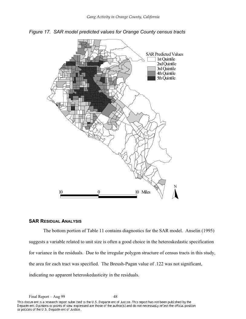
Gang Activity in Orange County, California
Figure 17. SAR model predicted values for Orange County census tracts
SAR Predicted Values1stQuintile2ndQuintile3rd Quintile4thQuintile5thQuintile
10 0 10 MilesN
SAR RESIDUAL ANALYSIS
The bottom portion of Table 11 contains diagnostics for the SAR model. Anselin (1995)
suggests a variable related to unit size is often a good choice in the heteroskedastic specification
for variance in the residuals. Due to the irregular polygon structure of census tracts in this study,
the area for each tract was specified. The Breush-Pagan value of .122 was not significant,
indicating no apparent heteroskedasticity in the residuals.
Final Report – Aug 99 48

Gang Activity in Orange County, California
The Likelihood Ratio (LR) test is an evaluation of the spatial lag variable for violent
crime. The LR test is equivalent to twice the difference between the log likelihood of the spatial
lag model and the log likelihood for the OLS regression model for violent gang incidents. This
test is significant, indicating that spatial lag has contributed significantly to the model.
The final diagnostic in Table 11 is the Lagrange Multiplier test for spatial error
dependence. The value of 0.121 is not significant, suggesting that spatial dependence is no
longer present in the model.
Figure 18 contains the Moran scatterplot of the residuals and associated spatial lag. The
Moran’s I coefficient of –0.007 is not significant (See bottom of Table 11).
Figure 18. Moran scatterplot of SAR residuals with regression line
SAR Residuals
4 3210-1-2-3-4
Spa
tial L
ag
2
1
0
-1
-2
The regression line from the regression used to calculate the Moran coefficient, which is
equivalent to the slope in a regression of residual spatial lag on the residuals, is provided in
Figure 18. Clearly, no detectable pattern is suggested in Figure 18 compared to the Moran
scatterplot for the OLS regression (see Figure 14).
Final Report – Aug 99 49

Gang Activity in Orange County, California
Figure 19 is a map of residuals from SAR model by Moran quadrant. The map is useful
for detecting the two types of positive spatial autocorrelation (large residuals surrounded by large
residuals and small residuals surrounded by small residuals) and corresponding negative spatial
autocorrelation (large residuals surrounded by small residuals or small residuals surrounded by
large).
Figure 19. SAR residuals by Moran Quadrant
SAR
Positive/PositivePositive/NegativeNegative/NegativeNegative/Positive
10 0 10 Miles
N
Residuals by Moran Quadrant
Final Report – Aug 99 50

Gang Activity in Orange County, California
Figure 20 is a map of significantly large residuals for the SAR regression model. There
are noticeably few large residuals present in the map for the SAR model. Compared to the map
in Figure 15 for the OLS model, there are fewer large positive or negative residuals spatially
grouped. Interestingly, the location of large residuals is in approximately the same location as
predicted by the OLS model.
Figure 20. Significantly large residuals for the SAR regression model
SAR Large Pos/Neg Residuals< -1.96 Std. Dev.> 1.96 Std. Dev.
10 0 10 MilesN
Final Report – Aug 99 51
Gang Activity in Orange County, California
CONCLUSIONS
The strength of the spatial relationship for violent gang incident results from OLS based
regression make them somewhat difficult to interpret. However, since the maximum likelihood
spatial autoregressive model was successful in reducing the spatial effect to an insignificant
level, the relationship between community structure and violent gang incidents can be safely
interpreted. Based on the findings of the SAR model, approximately 72 percent of the variance
in violent gang incidents can be explained by community structural characteristics, urbanization,
and the level of crime in neighboring communities. It appears that modern community-based
theories provide robust explanations for the relationship between communities and gang crime in
a region with many contiguous cities.
One of the strongest findings from the SAR model—and one with important policy
implications—is that communities tend to be significantly impacted by violent crime in
neighboring communities. Clearly, any attempt to reduce the gang problem in concentrated
areas within Orange County will have to consider neighboring communities as well. This means
that regional approaches such as the one mounted by the Orange County Chiefs’ and Sheriff’s
Association are required for tracking, understanding, or addressing street gang problems.
Although the aforementioned OLS regression model is similar to models found in other
studies (Schuerman and Kobrin, 1986; Messner and Sampson, 1991; Sampson and Grove 1989)
it should be interpreted with caution. Due to the level of spatial dependence, stemming from the
level of spatial autocorrelation in the dependent variable estimates for the coefficients will be
biased and any inference based on the t-tests and indication of fit from R2 are incorrect. As an
alternative, a spatial autoregressive model (SAR) is estimated which allows us to correctly
estimate the significance of the theoretical variables after controlling for spatial dependence.
Admittedly, the comparison of the two models suggests only minor differences in the degree of
Final Report – Aug 99 52

Gang Activity in Orange County, California
fit and the coefficients. Preliminary analysis revealed a number of individual indicators of
community structure to be unstable. Unique factors of community structure included in the OLS
and SAR models illustrate more stability since they have been generalized to represent those
characteristics that best represent the components of the community structure.
Using GITS to Evaluate the Effectiveness of Anti-Gang Strategies
INTRODUCTION
As part of a project funded by the USDOJ Community Oriented Policing Services Office
(COPS), a Tri-Agency Resource/Gang Enforcement (TARGET) Team12 was funded for the
Orange County city of Santa Ana. This brought the total number of TARGET Teams13 to four in
that city and 11 for the county as a whole. Each team is located in a specific police department
and consists of officers from that police department who serve as gang investigators, a probation
officer, a senior deputy district attorney and a district attorney’s investigator. The hallmark of
such teams is mutual cooperation across law enforcement agencies and vertical prosecution14
(see Kent and Smith, 1995). As part of the COPS grant the FRG was to explore the potential
usefulness of the GITS database for assessing TARGET Teams’ impact on gang activity. For
this analysis, the focus is only on the efforts in the City of Santa Ana.
TARGET Teams aim to suppress gang crime in Santa Ana through the efficient
identification, apprehension, and conviction of the violent gang leaders thought to be responsible
for much of the city’s gang problems. In the past, the usual method of determining the impact of
TARGET teams was to examine law enforcement records for changes in arrests, prosecutions,
convictions and sentencing. The GITS database also allows one to examine the impact of
12 For a description of TARGET Teams see Kent and Smith (1995). 13 In Santa Ana the TARGET Teams are called Street Terrorist Offender Programs (STOP).
Final Report – Aug 99 53

Gang Activity in Orange County, California
TARGET team activity on levels of gang activity within defined areas as well as effects on the
spatial distribution of gang incidents involving targeted gangs.
LAW ENFORCEMENT RECORD
Analyses of the TARGET Teams’ adjudication efforts use data on the prosecution of
targeted gang members. These data are compiled by the Orange County District Attorney’s
Office, and TARGET Teams also maintain records of each case handled by their prosecutors.
The District Attorney Office's report on the county TARGET Team efforts contains greater detail
on county-wide law enforcement statistics; what follows is a brief look at some of the statistics
for the city of Santa Ana.
In 1994, 1995, and 1996, the TARGET Teams reported substantial success in the arrest,
prosecution, and conviction of targeted gang offenders. After two years of targeting 42 members
of one Santa Ana gang, 28 members had been arrested, and 24 (86 percent) had been convicted
on a wide variety of charges. The average sentence length for all those convicted was 34 months
(not including one triple life sentence). After one year of targeting 20 members of another Santa
Ana gang, nine members had been arrested, and all nine had already been convicted within that
year. Not only are the cases of targeted gang members adjudicated quickly, conviction rates also
are high. As of December of 1996, only three of the targeted gang members who had been
arrested did not receive convictions.
In general TARGET teams throughout the county have managed to generate impressive
records with regard to both conviction rates and sentencing for individuals who have been
targeted. An alternative approach to evaluating TARGET teams is to look at their impact on
gang criminal activity.
14 Vertical prosecution refers to the Team’s continued and coordinated focus on an offender from level to level within the criminal justice system (e.g., from investigation through arrest and prosecution).
Final Report – Aug 99 54

Gang Activity in Orange County, California
USING GITS TO EVALUATE TARGET PERFORMANCE
Our knowledge of a TARGET Team’s ability to successfully convict and prosecute
targeted gang members is complimented nicely by evaluations of gang-related crime incidents in
Santa Ana. The analyses used here help us understand the relationship between the TARGET
team’s use of targeting strategies and actual levels of gang crime. As is shown below, the GITS
database makes several methods of analysis possible. Each method provides a unique view of
the relationship between gang crime and targeting. The effects of a TARGET team's efforts
against a particular gang can be examined from longitudinal trends in gang crime by comparing
pre- and post-targeting crime levels. Not only can changes in the annual number of incidents
committed by a gang be determined, but the nature of those incidents also can be examined. For
example, a gang may commit more incidents in a year following targeting, but the majority of
those incidents may be for less serious crimes than were committed before targeting. Because
the GITS database is longitudinal and because it contains many categories of variables, it is a
relatively straightforward task to build upon analyses in this manner. Clearly, doing so affords a
greater understanding of gang crime.
The following example focuses on the question, “What are the effects of targeting gang
rivalry, how does this affect criminal activity?” A related question concerns the possibility of
targeting impacting activity outside the targeting jurisdiction. That is, a gang that is targeted
may commit more or less crime in places outside the jurisdictional area of the TARGET Team.
Evaluations that consider only the amount of crime (not location) reported by the Santa Ana
Police Department may show a reduction in one targeted gang’s criminal activity, when in fact
the gang has reacted to police pressure and is offending in areas outside the city. Because gang
crime data from cities outside Santa Ana are not always readily available to the Santa Ana
TARGET Teams, if this is occurring, they may have inaccurate perceptions of their impact.
Final Report – Aug 99 55

Gang Activity in Orange County, California
Some of the gangs that have been targeted in Santa Ana are known to commit a majority
of their crimes in certain areas of the city. To demonstrate the use of GITS for monitoring the
spatial distribution of gang activity and targeting we focus on two active and violent gangs with
territories in Santa Ana, gang A and gang D.15 These gangs were long-time rivals with violent
histories of repeat offending and retaliation against one another. The TARGET team began
targeting gang D in 1995 in an attempt to ameliorate this rivalry. Given limited resources, it was
hoped that the targeting of one gang would remove some of its violent gang leaders from the
streets, which would directly impact on the level of activity for the targeted gang. This reduction
in gang presence was also intended to limit opportunities for inter-gang violence between gang D
and gang A and as a consequence impact the non-targeted rival gang A. The following maps
illustrate the effects of this strategy and help us understand whether targeting just one gang was
an effective way to interrupt the cycle of rivalry-related crime.
Figure 21 is a map of Santa Ana and surrounding areas that shows the turf of gang D and
gang A. Each point represents an incident of gang crime committed in 1994 by gang A. In
1994, when neither of the gangs was targeted, 88 percent of gang A's incidents (15 out of 17)
occurred in Santa Ana. Thirty-five percent of their incidents occurred on their own turf, six
percent occurred on rival gang D's turf, and only twelve percent occurred outside of Santa Ana.
Most of gang A's activity was restricted to Santa Ana (88 percent).
15 The Santa Ana Police Department has a policy of not using actual gang names in public reports because public exposure tends to enhance gang identity.
Final Report – Aug 99 56

Gang Activity in Orange County, California
Figure 21. Location of incidents committed by gang A in 1994
Figure 22 shows that during 1995, when gang D was targeted (but rival gang A was not),
the level of gang A's activity increased dramatically by 159 percent (from 17 to 44) but only 57
percent (25) now occurred in Santa Ana. While the proportion of gang A's activity on their turf
and gang D's turf dropped, the actual number stayed about the same. The major change occurred
in the actual increase in number of incidents both inside Santa Ana (but not on either A or D's
turf) and the number of incidents outside Santa Ana (an increase from two incidents to 19
incidents or 850 percent).
Final Report – Aug 99 57

Gang Activity in Orange County, California
Figure 22 Location of incidents committed by gang A in 1995. (Each dot may represent
more than one incident.)
Targeting of gang D was continued in 1996. At this point, because of continued rivalry
and a growing number of incidents as well as increased police resources, the decision was made
to also target the gang A directly. Figure 23 indicates that direct targeting further dispersed as
well as decreased gang A's activity. The number of incidents were decreased by 66 percent
(from 44 to15). By targeting gang A directly, its level of activity was brought back down to
where it was before the big increase in 1996 when rival gang D was targeted. The actual level of
activity outside of Santa Ana also decreased by 63 percent (from 19 to seven) but the pattern of
conducting a significant proportion of activity outside of Santa Ana, 47 percent, continued.
Final Report – Aug 99 58

Gang Activity in Orange County, California
Figure 23. Location of incidents committed by gang A in 1996
Spatial analysis of gang incidents clearly indicates the possibility of both direct and
indirect effects when a gang is targeted. Targeting gang A’s rival, gang D, is associated with
changes in the number and location of incidents involving gang A. Incidents involving gang A
increased, a greater proportion of their activity shifted to outside Santa Ana, and the proportion
of activity occurring on either gang’s turf diminished. When gang A was targeted directly, its
overall activity decreased dramatically both inside and outside Santa Ana. However, there still
was substantial activity outside Santa Ana. This example suggests that targeting a gang within
one city may affect its level of activity outside that city.16 Without county-wide data it is unlikely
that the Santa Ana TARGET Team would have been able to assess its impact on gang A this
completely.
16Of course other factors besides targeting, or interacting with targeting, may explain the geographic shift of incidents (e.g., increased recruitment of members outside Santa Ana or gang members moving outside the city.)
Final Report – Aug 99 59

Gang Activity in Orange County, California
ONGOING ANALYSES AND POLICY IMPLICATIONS
The county-wide data provided by GITS enable us to consider the activity of gangs in the
city where they are targeted. But they also let us look well beyond the city of origin. Our
ongoing analyses of crime committed by gangs A and D, as well as other targeted gangs, take
advantage of these comprehensive data. Density analyses are used to determine location of “hot-
spots” involving all gangs or particular gangs of interest. These analyses are provided to gang-
enforcement teams to judge whether they are targeting the most volatile areas of their cities.
Nearest-neighbor analyses also are being used to investigate spatial randomness of
incidents. For instance, it can be determine whether the activity of one gang is occurring
randomly within an expected area of activity, or if that gang is most likely to commit crime in
discrete locations. The spatial distribution of incidents around a point is being evaluated as well.
These analyses determine whether juvenile gang members, for example, are committing offenses
disproportionately around popular locations such as stores, schools, or parks.
Analyses such as these that currently are being conducted by the FRG appear very
promising for helping guide gang control policy and tactics at local and regional levels. GITS
data helps us understand the relationship between gang crime in Orange County and gang-
suppression efforts in a manner that would not be possible without such data. Individual law
enforcement agencies generally have data that are idiosyncratic, very limited in scope, and often
stored in formats that make empirical evaluation difficult. Given the limited (by location and
depth) data that individual departments may maintain, in-house analyses can lead to inaccurate
perceptions of gang crime, and thus to the implementation of misguided gang-suppression
strategies. Furthermore, police departments typically lack physical resources (e.g., software,
hardware) and skilled analysts to critically interpret the data that are available.
Final Report – Aug 99 60

Gang Activity in Orange County, California
OBJECTIVE 2: FEAR OF GANG CRIME
Our objective in this part of the research was to identify factors that contribute to
community members’ perceptions of—and fears about—gang violence. In order to determine
the accuracy of people’s perceptions of gang activities and their risks of becoming victims of
gang activities, we also compared residents’ reported fears to actual levels of gang activity in the
county as indicated by gang incidents reported by police. A final, and important, issue addressed
in this domain was how much perceptions about gang activities affected routine behavior and
quality of life. Dr. Jodi Lane was the team leader for this portion of the research.
Literature Review
Public opinion polls indicate that the fear of crime is increasing in the United States and
that people are modifying their behavior (e.g., including restricting nighttime activities and
avoiding shopping malls and parks) to escape becoming victims of crime (Baldassare and Katz,
1994, 1995, see also Miethe, 1995). There is evidence that recent increases in fear result mostly
from people’s fear of youth crime, and both media and police reports indicate that much of this
fear may result specifically from gang violence. As Lewis and Maxfield (1980: 184) note, “Fear
of crime may be directly affected by concern about local adolescents.” This fear of youthful
offenders is likely to become even more important as communities that previously considered
themselves immune from gang violence are forced to face gangs moving beyond the inner city
and extending into previously untouched neighborhoods (Curry, Ball, and Fox, 1994; Spergel
and Curry, 1995).
Although statistics show that some types of crime are increasing (e.g., youth violence),
overall crime trends suggest we are not experiencing a surge of crime that would explain recent
Final Report – Aug 99 61

Gang Activity in Orange County, California
steep increases in public fear (Ferraro, 1995; Lewis and Maxfield, 1980; Taylor & Hale, 1986;
Taylor & Shumaker, 1990; Tyler, 1980). In fact, overall crime levels in Orange County dropped
14 percent in 1994 and crime rates in California dropped to the lowest level in a decade. The
number of crimes in all major categories (including homicide, rape, robbery, assault, burglary
and automobile theft) decreased during this period (Los Angeles Times, 1995). Crime has
continued to drop during each year since 1994 (Grad and Hua 1997: A1). In other words, fear of
crime appears to be based on something other than crime rates.
This accelerating yet apparently unrealistic fear of crime is an important subject of study
for two reasons. First, because it can have a number of psychological and behavioral
consequences for individuals who are fearful (e.g., Liska, Sanchirico, and Reed, 1988; Liska and
Warner, 1991; Miethe, 1995; Ross, 1993; Taylor and Shumaker, 1990). Second, because public
opinion is critically important in driving public policy (e.g., Lewis and Maxfield, 1980; Taylor
and Hale, 1986; Warr, 1994). Recently, fear of crime has resulted in the passage of harsh
mandatory sentencing policies (so-called ‘Three Strikes and You’re Out’ initiatives) that so far
have increased prison populations drastically without creating a substantial reduction in crime
(Blumstein, 1995). This substantial increase in prisoners pulls funds away from other needed
social services like prevention programs, schools, and child health care (Vila 1997a, 1997b). Yet
the public demands more incarceration, in part because they are afraid of crime. It doesn’t
appear possible for state governments to continue to answer public calls for harsher prison
sentences when there is little evidence that indiscriminate increases in imprisonment cause
significant decreases in crime (see Greenwood et al., 1996; Greenwood et al., 1994; Spelman,
1994; Zimring, 1995). Thus it seems particularly important to understand and attempt to
alleviate factors that contribute to disproportionate public fear of crime.
Final Report – Aug 99 62

Gang Activity in Orange County, California
Since the 1970s, criminologists have made substantial progress toward understanding the
incongruence between fear levels and actual criminal victimizations. These studies have mostly
analyzed official data (e.g., reported crime and arrest rates) and correlated overall crime
indicators with information on resident characteristics (e.g., age, gender, race, income level, prior
victimization) and reported fear levels, which generally have been measured through public
opinion surveys (typically random telephone surveys). Although there have been “a bewildering
variety of questions [employed] to measure fear,” most of these studies have relied on the
standard, well-known fear of crime survey questions used by the General Social Survey (GSS)
and Gallup (Warr, 1994: 6-7). Questions asked include, for example, “How safe do you feel or
would you feel being out alone in your neighborhood at night?”17 There has been considerable
debate over the validity and reliability of the GSS and Gallup questions in measuring fear of
crime (see DuBow et al., 1979; LaGrange and Ferraro, 1987). As Warr (1994: 7) notes, these
standard questions are better suited for measuring the prevalence rather than the magnitude of
fear and have the major limitation of not indicating exactly what people “are afraid of.” Further,
as Warr and Stafford (1983) indicate, the seriousness of the crime and one’s perceived risk of
being victimized also may be important to understanding how these questions are answered.
However, we have a relatively good understanding of the prevalence of fear and its demographic
correlates because the standard questions and trends have been used for decades.
During the 1970s and 1980s, about one-third to one-half of Americans reported that they
were afraid of crime. However, fear of crime began to increase during the 1990s (Baldassare and
Katz, 1994, 1995). Individual characteristics that are important for predicting reported fear of
17 This question typically is used in the National Crime Survey (Ferraro, 1995; LaGrange and Ferraro, 1989). Although the wording of the GSS question varies, it generally reads: “Is there any area around here—that is, within a mile—where you would be afraid to walk alone at night (or during the day)?” (Ferraro, 1995; Warr, 1994: 6; Yin, 1985).
Final Report – Aug 99 63

Gang Activity in Orange County, California
crime include age, gender, race, income level, and victimization. In general, studies have found
that women and older individuals are more afraid than males and younger people, even though
women and the elderly face the lowest objective risk of victimization (Baumer, 1978; Ferraro,
1995; Garofalo and Laub, 1978; Miethe, 1995; Riger, Gordon and Le Bailly, 1978). However
the findings for age effects are not consistent, some have argued that the elderly are not
necessarily as fearful as many assume (see Ferraro and LaGrange 1987, 1988; LaGrange et al.
1992; McCoy et al. 1996). It also is possible that the disproportionate reporting of fear among
groups that are less likely to be victimized reflects perceptions about ability to bear the
consequences of victimization. For example, an elderly person who is beaten may be disabled
for the rest of his or her life while a young man receiving a similar beating may recover in a
matter of days.
Minorities (especially African-Americans) are typically more fearful than whites
(Baumer, 1978; Skogan, 1995; Warr, 1994). People who live in low-income areas also typically
are thought to be more fearful, although the evidence here is inconclusive (Taylor and
Covington, 1993; Warr, 1994; Will and McGrath, 1995). The relationship between prior
victimization and fear is likewise problematic in that those most victimized are not necessarily
most fearful (Garofalo, 1979; Garofalo and Laub, 1978; Taylor and Hale, 1986; Warr, 1994).
Recognizing that the demographic characteristics most closely associated with fear do not
necessarily correspond with likelihood of victimization, studies now typically analyze
community characteristics that may help explain this discrepancy. In general, urban residents are
more fearful than people who live in rural areas (Boggs, 1971, Warr, 1994), and people who live
in larger cities tend to be more fearful than those who live in smaller ones (Clemente and
Kleinman, 1977). Residents in areas with more racial heterogeneity and higher poverty levels
Final Report – Aug 99 64

Gang Activity in Orange County, California
also tend to report more fear (Covington and Taylor, 1991; Lizotte and Bordua, 1980; Merry,
1981; Skogan, 1995; Will and McGrath, 1995)—purportedly because they are more likely to
have direct experience with crime and with incivilities (Ferraro, 1995).
Other community characteristics hypothesized to be crucial in explaining fear of crime
include public disorder and/or community decline. Disorder, as indicated by social (e.g.,
loitering or rowdy youths, drunks, prostitution) and physical incivilities (e.g., litter, vacant
buildings, abandoned lots, broken windows, graffiti), is often found to lead to and increase fear
(e.g., Lewis and Maxfield, 1980; Perkins et al., 1992; Taylor, 1991; Taylor and Shumaker, 1990;
Taylor, Shumaker, and Gottfredson, 1985; Wilson and Kelling, 1982). Another important
predictor of fear is concern over community decline and deterioration (see Conklin, 1975;
Garofalo and Laub, 1978). Including community variables has added an important dimension to
research on fear of crime, suggesting it is influenced not simply by personal characteristics, but
also by the relationship between personal characteristics, community characteristics, and actual
crime victimization probabilities.
There currently are four dominant theoretical models that incorporate both individual and
community correlates of fear of crime: indirect victimization, incivilities, community concern
(decline) and subcultural diversity/racial heterogeneity (Covington and Taylor, 1991).
• “Indirect victimization” refers to the idea that people hear about crime through local
social networks and through the media and consequently experience vicarious
victimization which makes them fearful (Skogan, 1977; Tyler, 1980).
• “Incivilities” refers the idea that when community members perceive social and physical
signs of an “underlying level of disorder” in their immediate surroundings, they feel more
vulnerable and therefore more fearful (e.g., Covington and Taylor, 1991: 232; see also
Lewis and Maxfield, 1980; Taylor, 1991).
Final Report – Aug 99 65
Gang Activity in Orange County, California
• “Community concern” argues that fear of crime is primarily the result of concern over
community deterioration (Conklin, 1975; Covington and Taylor, 1991; Garofalo and
Laub, 1978).
• “Subcultural diversity” argues that individuals who live near people of different cultural
(or racial) backgrounds are more fearful because they find it difficult to interpret the
manners and behaviors of people who are different from themselves (Merry, 1981; see
also Skogan, 1995).
Covington and Taylor (1991) found support for aspects of all four models but even using
expanded models, they were unable to explain much of the variance in the fear of crime
phenomenon. At best, these types of models explain only about 10 percent of the variance
(Covington and Taylor, 1991; Taylor and Hale, 1986). To date, no study has tested the
applicability of these models to fear of youth and street gangs. We believe that such a focus is
particularly important to the study of community characteristics and their relationship to fear of
crime. As noted earlier, gang membership and violence are believed to be on the rise, and
communities that have never experienced gang crime now are being forced to confront it. Media
reports heinous and seemingly random crimes committed by young people such as the murder of
a 3-year-old girl in Los Angeles whose family members took a wrong turn into a “gang-infested”
neighborhood, seem likely to exacerbate fear of gangs.
Fear of Crime and Gangs Survey Methods
CONDUCTING THE SURVEY
From September 3–28, 1997, we conducted a random digit dial survey of 1,000 Orange
County residents with a 50-50 split between men and women.18 In addition to the random
sample, we sampled 100 Hispanic and 100 Vietnamese county residents to allow for smaller
Final Report – Aug 99 66

Gang Activity in Orange County, California
analyses of fear of crime and gangs in these large ethnic groups. The survey had a total of 1,200
respondents and took approximately 20 minutes to administer. The random digit dial portion of
the survey broadly reflects the ethnic distribution of the county: 63 percent white, 18 percent
Hispanic, 6 percent Asian-American and 9 percent others.
The survey instrument itself was designed to measure the level of fear in the community
with regard to gangs and gang crime, investigate the theoretical factors related to fear, and relate
these perceptions to variations in crime across the county. To measure prevalence of fear, for
example, we asked if gangs were a problem in the community, if so, when they became a
problem, and if respondents believed that different types of crime had increased or decreased in
recent years. We also measured behavioral reactions to fear of gangs, such as avoiding certain
areas of the community and carrying a weapon for protection (see Appendix B).
We also hoped to measure theoretical propositions put forth by fear of crime researchers
about the causes of fear (see above). For example, one section of the survey measured concern
about community problems such as disorder/incivilities, community decline, and subcultural
diversity/racial heterogeneity. We also wanted to examine Warr and Stafford’s (1983)
proposition that fear is at least correlated with one’s perception of the crime’s seriousness and
the perceived risk of victimization. This required us to examine specific criminal acts rather than
just generalized perceptions of crime. Therefore, for eight different crimes (six personal and two
property), we asked respondents to indicate the seriousness, the likelihood that they would be
victimized by that crime in the next two to three years, and how personally afraid they were of
that crime. Since the focus of this study is on gang crime, six of the eight crimes were specified
as gang crimes or were crimes typically associated with gang members. These six crimes were:
18 We contracted with Interviewing Services of America in Van Nuys, California to administer the survey. Interviews were closely monitored by Dr. Jodi Lane, the lead researcher on this aspect of our project.
Final Report – Aug 99 67

Gang Activity in Orange County, California
• Having your property damaged by gang graffiti or tagging
• Having a gang member commit a home invasion robbery against you
• Being a victim of a drive-by or random gang-related shooting
• Being physically assaulted by a gang member
• Being harassed by gang members
• Being a victim of a carjacking
The other two crimes in the list were:
• Having someone break into your home while you are away
• Being raped or sexually assaulted by a stranger
The general burglary question was included to allow us to compare fear of gang crimes with fear
of a crime not necessarily associated with gangs. Rape was included to allow us to control for
fear of rape in understanding women’s fear of crime in later analyses.
In addition to measuring fear of crime and gangs, the survey measured respondents’
concern about community-level problems which theorists have noted are important to predicting
fear of crime. The question asked:
We have a number of questions about your community as you define it. I will
read you a list of some things that currently might be problems in your community. After
I read each one, please tell me whether you think it is a big problem, somewhat of a
problem, a small problem, or no problem in your community.19
Some of the community problems listed overlap constructs from different theories
about community effects and therefore can be included as measures of more than one
theory. The questions and the theoretical constructs they were designed to measure are
listed in Table 12.
Final Report – Aug 99 68

Gang Activity in Orange County, California
Table 12. Theoretical constructs and survey questions used to measure them
THEORETICAL CONSTRUCT COMMUNITY PROBLEM QUESTION(S)
DISORDER
Social Disorganization:
• Poverty and economic hardship
• People moving in and out without personally
becoming attached to the community
• Racial differences between residents
Physical Incivilities:
•
•
•
•
•
•
People or landlords allowing their property to
become run down
Abandoned houses or other empty buildings
Graffiti
Social Incivilities:
Too many people living in one residence
Youths hanging out
Gangs
COMMUNITY DECLINE
•
•
•
•
•
•
•
People or landlords allowing their property to
become run down
People moving in and out without personally
becoming attached to the community
Abandoned houses or other empty buildings
Graffiti
Too many people living in one residence
Youths hanging out
Gangs
SUBCULTURAL DIVERSITY/ RACIAL HETEROGENEITY
•
•
•
•
Language differences between residents
Cultural differences between residents
Racial differences between residents
Too many people living in one residence20
19 An earlier question asked respondents to indicate how they defined their community. 20 This question is included as a measurement of this construct because another study of fear in Orange County using focus groups with residents of six Santa Ana, California, neighborhoods indicated that residents associated their neighborhood crime and gang problems and therefore their fear of them with Hispanic immigrants. Part of the
Final Report – Aug 99 69

Gang Activity in Orange County, California
Analysis of Random Digit Dial Survey Findings
To ensure that our analysis applies to the county at large, much of what we report here
deals only with the random digit dial sample of 500 men and 500 women. The research
questions presented in this section will report analysis and findings from these 1,000
respondents. Later, we will examine the differences in fear of crime and gangs between the
subsamples of whites, Hispanics, and Vietnamese residents.
HOW MUCH FEAR DO RESIDENTS CURRENTLY HAVE ABOUT GANG VIOLENCE?
As noted above, the survey asked respondents to indicate on a 4-point scale personal
perceptions about seriousness, risk, and fear regarding eight different crimes.21 Tables 13-15
provide the percentages of the random digit dial sample respondents who answered in each of the
four category options for each of the eight crimes. The tables rank order crimes from most to
least serious, likely to occur, or fear provoking.
problem according to these respondents was that Hispanic immigrants often lived with multiple families in one household, which often led to more neighborhood disorder (Lane 1998). 21 The order of these crimes was rotated randomly during the survey to control for response effects.
Final Report – Aug 99 70

Gang Activity in Orange County, California
Table 13. RDD respondents rank the seriousness of eight crimes
CRIMES:
n
NOT SERIOUS
(%)
SOMEWHAT SERIOUS
(%)
SERIOUS
(%) VERY
SERIOUS
(%)
MEAN
95% CONFIDENCE
INTERVAL
PROPERTY CRIMES:
Burglary 996 7.9 11.3 33.1 47.6 3.20 3.15–3.26
Graffiti 998 11.5 20.7 34.7 33.1 2.89 2.83–2.95
PERSONAL CRIMES:
Rape 994 8.6 3.2 5.9 82.3 3.62 3.56–3.68
Drive-By/Random Gang Shooting 998 9.7 3.1 6.8 80.4 3.58 3.52–3.64
Gang-Related Assault 997 9.4 3.8 12.2 74.5 3.52 3.46–3.58
Home Invasion Robbery 995 9.2 4.3 15.6 70.9 3.48 3.42–3.54
Carjacking 996 9.0 5.9 18.8 66.3 3.42 3.36–3.48
Gang-Related Harassment 995 10.9 13.5 34.5 41.2 3.06 3.00–3.12
Final Report – Aug 99 71

Gang Activity in Orange County, California
Table 14. RDD respondents indicate the likelihood that they will become a victim of eight crimes in the next 2-
3 years
CRIMES:
n
NOT LIKELY
(%)
SOMEWHAT LIKELY
(%)
LIKELY (%)
VERY LIKELY
(%)
MEAN
95% CONFIDENCE
INTERVAL
PROPERTY CRIMES:
Burglary 983 37.1 40.2 17.4 5.3 1.91 1.85–1.96
Graffiti 985 57.6 26.0 9.9 6.5 1.65 1.60–1.71
PERSONAL CRIMES:
Rape 980 49.2 33.6 12.3 4.9 1.73 1.68–1.78
Drive-By/Random Gang Shooting 985 55.7 27.4 12.2 4.7 1.66 1.60–1.71
Gang-Related Assault 979 59.3 26.9 9.9 3.9 1.58 1.53–1.63
Home Invasion Robbery 981 61.6 24.2 9.8 4.5 1.57 1.52–1.62
Carjacking 981 63.3 23.6 7.6 5.4 1.55 1.50–1.60
Gang-Related Harassment 982 69.2 19.0 7.2 4.5 1.47 1.42–1.52
Final Report – Aug 99 72

Gang Activity in Orange County, California
Table 15. RDD respondents indicate how personally afraid they are of eight crimes
CRIMES:
n
NOT AFRAID
(%)
SOMEWHAT AFRAID
(%)
AFRAID (%)
VERY AFRAID
(%)
MEAN
95% CONFIDENCE
INTERVAL
PROPERTY CRIMES:
Burglary 995 29.3 37.3 16.3 17.1 2.21 2.15–2.28
Graffiti 994 47.9 26.8 14.5 10.9 1.88 1.82–1.95
PERSONAL CRIMES:
Rape 994 35.5 23.8 13.0 27.7 2.33 2.25–2.40
Drive-By/Random Gang Shooting 995 32.5 29.0 13.6 24.9 2.31 2.24–2.38
Gang-Related Assault 994 42.4 16.4 10.6 30.7 2.30 2.22–2.38
Home Invasion Robbery 993 37.5 24.1 12.3 26.2 2.27 2.20–2.35
Carjacking 995 36.4 24.5 14.6 24.5 2.27 2.20–2.35
Gang-Related Harassment 995 41.5 28.4 14.2 15.9 2.04 1.98–2.11
Final Report – Aug 99 73

Gang Activity in Orange County, California
COMPARING THE PERCENTAGES
Based upon the percentages presented in the above three tables, there are clear
differences between respondents’ ratings of the seriousness of these crimes, their perceived risk
of victimization and their personal fear of them. In general, respondents see personal crimes as
serious but have a low perceived risk and are only “somewhat afraid.” However, an examination
of the percentages by type of crime indicates that ratings of seriousness, perceived risk, and fear
are very different. For example, for the property crimes of tagging/graffiti and burglary, about
one-third to one-half thought the crimes were very serious, about 5-7 percent felt very likely it
would happen to them, and 10–20 percent were very afraid of them. For gang-related assault,
74.5 percent of respondents felt it was “very serious,” but only 4.5 percent felt that it was “very
likely” to happen to them in the next two to three years and about 26.2 percent of them were
“very afraid” of gang assault. For the “random” crimes often focused on by the media such as
drive-by shootings, carjacking, and home invasion robbery there also were clear differences.
Although a strong majority felt that these crimes were very serious, only about a quarter of
respondents were “very afraid” of them, and most of them did not think that they were very
likely to be victimized by these serious violent crimes—even though they were “random” and
theoretically could happen to anyone. Interestingly, rape was ranked as the most serious crime in
the list, but was seen as the least likely, and ranked in the middle in terms of fear.22
These data only provide partial support for Warr and Stafford’s (1983) proposition that
fear is correlated with one’s perception of crime seriousness and perceived risk of victimization.
For personal crime, the relative rank order for risk, seriousness and fear are the same indicating
association. Property crime, on the other hand, follows a core couples relationship. Both
burglary and graffiti are seen in terms of low fear and seriousness, but very likely for
Final Report – Aug 99 74

Gang Activity in Orange County, California
victimization. A more sophisticated analysis of Warr and Stafford’s (1983) propositions follows
later.
FACTORS AFFECTING RESIDENTS’ PERCEPTIONS AND FEARS REGARDING GANG ACTIVITY
Importance of Demographics
The foregoing tables indicate differences between people’s perceptions about seriousness,
risk, and fear of the eight crimes. It also is important to know what factors are most likely to
predict feelings about these eight crimes. Past research has shown that demographics —
especially age and gender—are important predictors of fear and have emphasized the importance
of subjective concern about community problems such as disorder and community decline. To
better understand the relationship between demographics and concern about community
problems, we conducted regressions predicting seriousness, perceived risk, and fear for each of
the eight crimes based upon demographic characteristics other than race/ethnicity (Tables 16-18).
22 For this table, both men and women’s assessments of rape are included.
Final Report – Aug 99 75

Gang Activity in Orange County, California
Table 16. Predicting crime seriousness ranking based upon RDD respondent
demographic characteristics
SERIOUSNESS23
DEMOGRAPHICS GRF BRG HAR ASS CRJ HNV DBY RAP
SEX24 .226**
(.115)
.133*
(.072)
.275***
(.140)
.241***
(.129)
.082
(.043)
.177**
(.095)
.201**
(.106)
.199**
(.112)
AGE -.043
(-.068)
-.019
(-.033)
-.033
(-.051)
-.056**
(-.093)
-.055*
(-.091)
-.042*
(-.070)
-.037
(-.060)
-.039
(-.068)
INCOME .024
(.047)
.034
(.071)
.040
(.078)
.051**
(.106)
.056**
(.114)
.030
(.061)
.031
(.064)
.039*
(.084)
EDUCATION -.030
(-.040)
-.027
(-.038)
-.051
(-.067)
.069*
(096)
.019
(.026)
.055
(.077)
.027
(.037)
.047
(.068)
VICTIM25 .005
(.002)
.163
(.074)
.028
(.012)
.019
(.008)
.059
(.026)
.104
(.047)
.152
(.068)
.073
(.035)
R2 .018 .015 .026 .049 .025 .028 .026 .032
R2 ADJ .012 .009 .020 .043 .020 .022 .020 .026
F 3.104** 2.587* 4.375** 8.592*** 4.332** 4.701*** 4.376** 5.508***
Df 5, 830 5, 829 5, 827 5, 830 5, 829 5, 827 5, 830 5, 827
B (Beta) * p < .05 ** p < .01 *** p < .001; 1000 Respondents, 500 Men, 500 Women
23 GRF = graffiti or tagging, BRG = burglary, HAR = harassment by gang members, ASS = physical attack or assault by a gang member, CRJ = carjacking, HNV = home invasion robbery, DBY = drive-by or random gang-related shooting, RAP = rape. 24 Gender is dummy coded. 1= female, 0 = male. 25 Victimization is dummy coded with 1 equaling some type of personal victimization by crime in the past 2 to 3 years, and 0 equaling no personal victimization in the past 2 to 3 years.
Final Report – Aug 99 76

Gang Activity in Orange County, California
Table 17. Predicting perceived risk of victimization based upon RDD respondent
demographic characteristics
PERCEIVED RISK26
DEMOGRAPHICS GRF BRG HAR ASS CRJ HNV DBY RAP
SEX27 .066
(.037)
.136*
(.080)
-.007
(-.004)
-.019
(-.011)
.041
(.024)
.076
(.047)
.092
(.055)
.354***
(.222)
AGE -.058**
(-.100)
-.037
(-.067)
-.072***
(-.130)
-.057*
(-.107)
-.022
(-.040)
-.028
(-.054)
-.014
(-.026)
-.027
(-.052)
INCOME -.069***
(-.148)
-.018
(-.041)
-.037*
(-.082)
-.064***
(-.148)
-.030
(-.068)
-.063***
(-.151)
-.065***
(-.149)
-.042*
(-.101)
EDUCATION -.080**
(-.116)
-.036
(-.055)
-.101***
(-.153)
-.139***
(-.219)
-.122***
(-.188)
-.085***
(-.137)
-.116***
(-.181)
-.101***
(-.165)
VICTIM28 .296
(.138)
.222**
(.110)
.427***
(.209)
.217**
(.109)
.182**
(.091)
.258***
(.135)
.153*
(.077)
.160*
(.084)
R2 .093 .033 .118 .138 .067 .092 .096 .120
R2 ADJ .088 .028 .113 .133 .062 .086 .091 .115
F 16.91*** 5.69*** 22.05*** 26.23*** 11.82*** 16.54*** 17.40*** 22.36***
Df 5, 824 5, 821 5, 824 5, 818 5, 819 5, 818 5, 819 5, 819
B (Beta) * p < .05 ** p < .01 *** p < .001; 1000 Respondents, 500 Men, 500 Women
26 GRF = graffiti or tagging, BRG = burglary, HAR = harassment by gang members, ASS = physical attack or assault by a gang member, CRJ = carjacking, HNV = home invasion robbery, DBY = drive-by or random gang-related shooting, RAP = rape. 27 Gender is dummy coded. 1= female, 0 = male. 28 Victimization is dummy coded with 1 equaling some type of personal victimization by crime in the past 2 to 3 years, and 0 equaling no personal victimization in the past 2 to 3 years.
Final Report – Aug 99 77

Gang Activity in Orange County, California
Table 18. Predicting personal fear based upon RDD respondent demographic
characteristics
FEAR29
DEMOGRAPHICS GRF BRG HAR ASS CRJ HNV DBY RAP
SEX30 .374***
(.184)
.405***
(.196)
.593***
(.274)
.678***
(.282)
.631***
(.271)
.549***
(.231)
.549***
(.226)
1.165***
(.451)
AGE -.013
(-.020)
-.011
(-.017)
-.046
(-.066)
-.010***
(-.128)
-.064*
(-.085)
-.062*
(-.080)
-.088**
(-.113)
-.130***
(-.156)
INCOME -.023
(-.043)
-.010
(-.019)
-.007
(-.012)
-.001
(-.001)
.018
(.029)
-.006
(-.010)
-.019
(-.030)
-.009
(-.014)
EDUCATION -.105**
(-.135)
-.083**
(-.105)
-.106**
(-.127)
-.073*
(-.079)
-.075*
(-.084)
-.079*
(-.087)
-.107**
(-.115)
-.079*
(-.079)
VICTIM31 -.040
(-.017)
.087
(.035)
.037
(.014)
.089
(.031)
.155
(.056)
.148
(.052)
-.054
(.019)
.042
(.014)
R2 .062 .054 .098 .102 .088 .072 .083 .230
R2 ADJ .056 .049 .092 .096 .083 .067 .078 .225
F 10.87*** 9.52*** 17.93*** 18.76*** 16.05*** 12.91*** 15.06*** 49.43***
Df 5, 828 5, 829 5, 828 5, 828 5, 828 5, 828 5, 828 5, 829
B (Beta) * p < .05 ** p < .01 *** p < .001; 1000 Respondents, 500 Men, 500 Women
Tables 16-18 again support the notion that predictors of fear of crime, as well as
seriousness and perceived risk, differ depending upon the type of crime. For crime seriousness,
which is presented in Table 16, gender (being female) is significantly related to ratings for every
crime except carjacking. Age also is significantly and negatively related to ratings of seriousness
for gang-related assault, carjacking, and home invasion robbery. Income is significantly and
29 GRF = graffiti or tagging, BRG = burglary, HAR = harassment by gang members, ASS = physical attack or assault by a gang member, CRJ = carjacking, HNV = home invasion robbery, DBY = drive-by or random gang-related shooting, RAP = rape. 30 Gender is dummy coded. 1= female, 0 = male. 31 Victimization is dummy coded with 1 equaling some type of personal victimization by crime in the past 2 to 3 years, and 0 equaling no personal victimization in the past 2 to 3 years.
Final Report – Aug 99 78

Gang Activity in Orange County, California
positively related to seriousness ratings for gang-related assault, carjacking, and rape.
Interestingly, education is significantly and positively related only to ratings of the seriousness of
gang-related assault. Previous victimization is not significantly related to seriousness ratings for
any of the crimes.
Table 17 presents results of regression analyses predicting perceived risk for each of the
eight crimes based upon respondent’s demographic characteristics. For perceived risk, being
female is positively and significantly related to rape and burglary. Age is significantly and
negatively related to perceived risk of graffiti, gang-related harassment, and gang-related assault.
Income is significantly and negatively related to perceived risk of graffiti, gang-related
harassment, gang-related assault, home invasion robbery, drive-by shootings, and rape.
Education is significantly and negatively related to perceived risk of all crimes except burglary.
And prior victimization is significantly and positively related to perceived risk of burglary, gang-
related harassment and assault, carjacking, home invasion robbery, drive-bys and rape.
Table 18 presents results of regression analyses predicting fear of crime from
demographic characteristics. Consistent with most of the previous literature, being female is
significantly and positively related to reported fear of all eight crimes. On the other hand, unlike
findings from most studies, our analyses indicate that, in Orange County at least, younger (rather
than older) people are significantly more likely to be afraid of gang-related assault, carjacking,
home invasion robbery, drive-by shootings, and rape. Education is significantly and negatively
related to fear of all eight crimes. Interestingly, income and victimization are not significantly
related to fear of any of the crimes.
Final Report – Aug 99 79

Gang Activity in Orange County, California
COMPARING EFFECTS OF DEMOGRAPHICS ON SERIOUSNESS, PERCEIVED RISK, AND FEAR
Tables 16–18 show that predictors of seriousness, perceived risk, and fear vary depending
upon the type of crime. In addition, perceived risk and personal fear clearly are not the same
phenomena. Here, gender (being female)—one of the strongest predictors of fear in previous
research (Baumer 1978; Ferraro 1995; Garofalo and Laub 1978; Miethe 1995; Riger, Gordon
and Le Bailly 1978)—again is significantly related to fear of all types of crime included in the
survey. It also is significantly related to seriousness ratings for all crimes except carjacking.
However, gender is significantly related to the perceived risk for only two crimes—burglary and
rape, the two crimes that are not necessarily “gang-related.”
Age is negatively and significantly related to fear of gang-related assault, carjacking,
home invasion robbery, drive-by shootings, and rape. Although many studies have found a
positive relationship between age and fear, our finding is not unique (see Ferraro and LaGrange
1987, 1988; LaGrange et al. 1992; McCoy et al. 1996). Age also is negatively related to
perceived risk of graffiti, gang harassment, and gang-related assault. In Orange County, it
appears younger people are more likely to fear these crimes and to believe they are more likely
to become victims of them.
Previous findings that poverty is positively related to fear (Taylor and Covington 1993;
Warr 1994; Will and McGrath 1995) receive mixed support here. Income is positively and
significantly related to perceptions of the seriousness of gang-related assault, carjacking, and
rape, but it is negatively and significantly related to perceived risk of graffiti, gang harassment,
gang assault, home invasion, drive-bys and rape. However, it is not significantly related to fear
for any of the crimes. Education shows the same pattern, although it is significantly and
negatively related to fear of all eight crimes. For seriousness, education is positively and
significantly related to gang assault, but for perceived risk it is negatively and significantly
Final Report – Aug 99 80

Gang Activity in Orange County, California
related to graffiti, gang harassment, gang assault, carjacking, home invasion robbery, drive-bys,
and rape. As some previous research has indicated, personal victimization within the past two to
three years is not a significant predictor of fear of any of the crimes. Nor is it predictive of
seriousness ratings for them. However, it is significantly related to perceived risk of all the
crimes except burglary.32
Because previous studies have indicated that fear and actual victimization risk based
upon demographic characteristics do not coincide, fear of crime theorists have emphasized the
importance of measuring concern about community problems like disorder, community decline,
and subcultural diversity/racial heterogeneity as important factors in predicting fear. As noted
previously, our survey was designed to measure all three theories, but a factor analysis indicated
the presence of two, rather than three, factors. The survey data loaded primarily on a “disorder”
factor and a “diversity” factor. The failure of community decline to emerge as a coherent factor
may have occurred because many of the variables indicative of concern about disorder also
indicate concerns about community decline. The factors that emerged are:33
DISORDER DIVERSITY • •
• • • • •
• • • •
Poverty and economic hardship People or landlords allowing their property to become run down Abandoned houses or other empty buildings Gunfire Graffiti Gangs Youths hanging out
Language differences between residents Cultural differences between residents Racial differences between residents People moving in and out without becoming attached to the community
We developed composite variables in order to enter the disorder and diversity constructs
into regression equations by computing arithmetic averages for each respondent, summing the
scores for all variables in the factor, and dividing by the number of variables (seven for disorder
32 The direction of relationships in the multiple regression analysis are consistent with the direction of relationships for the bivariate correlations.
Final Report – Aug 99 81

Gang Activity in Orange County, California
and four for diversity). We then computed the same regressions as before with the addition of
disorder and diversity variables. Tables 19–21 show the results of these the regression analyses.
Table 19. Predicted perceptions of seriousness based upon demographic, disorder,
and diversity variables
SERIOUSNESS 34
VARIABLES GRF BRG HAR ASS CRJ HNV DBY RAP STEP 1
.216** .176** .306*** .280*** .127 .230** .218** .242*** SEX (.110) (.095) (.158) (.149) (.067) (.122) (.115) (.135)
-.034 -.013 -.005 -.038 -.049* -.033 -.024 -.029 AGE (-.053) (-.021) (-.007) (-.061) (-.079) (-.053) (-.039) (-.048)
.032 .041* .053* .056** .058** .044* .043* .056** INCOME (.063) (.085) (.104) (.113) (.117) (.088) (.086) (.119)
-.006 -.010 -.038 .070* .028 .059 .030 .038 EDUCATION (-.007) (-.014) (-.050) (.094) (.038) (.079) (.040) (.055)
.004 .181* .041 .035 .054 .096 .146 .080 VICTIM (.002) (.082) (.018) (.016) (.024) (.043) (.064) (.037)
STEP 2 DISORDER .149*
(.126)
.103
(.092)
.150**
(.128)
.067
(.059)
.080
(.070)
.094
(.082)
.023
(.020)
.070
(.065)
DIVERSITY -.015
(-.012)
-.075
(-.063)
.000
(.000)
.017
(.014)
-.017 -.037
(-.030)
.047
(.038)
.039
(.705)
R2 CHANGE STEP 1
.016* .021** .030*** .048*** .025** .033*** .029** .038***
R2 CHANGE STEP 2
.013** .005 .015** .004 .004 .004 .003 .008
MODEL R2 .029 .025 .045 .053 .028 .037 .031 .046
MODEL R2 ADJ .020 .016 .036 .044 .019 .028 .022 .037
MODEL F 3.232** 2.764** 5.029 5.960**
*
3.127** 4.117**
*
3.458** 5.095**
*
MODEL df 7, 749 7, 748 7, 748 7, 749 7, 748 7, 747 7, 749 7, 746
(-.014)
B (Beta) from final model including both steps * p < .05 ** p < .01 *** p < .001
33 The alpha for the disorder scale is .9059 and for the diversity scale is .7752.
Final Report – Aug 99 82

Gang Activity in Orange County, California
Table 20. Predicted perceived risk of victimization based upon demographic, disorder,
and diversity variables
PERCEIVED RISK35
VARIABLES GRF BRG HAR ASS CRJ HNV DBY RAP
STEP 1
SEX .075
(.043)
.141*
(.086)
.007
(.004)
-.012
(-.007)
.044
(.027)
.073
(.048)
.098
(.062)
.347***
(.221)
AGE -.036
(-.063)
-.025
(-.046)
-.039*
(-.072)
-.029
(-.056)
.007
(.012)
-.009
(-.017)
.022
(.041)
-.009
(-.017)
INCOME -.054**
(-.119)
-.000
(.000)
-.014
(-.034)
-.044**
(-.105)
-.016
(-.037)
-.048**
(-.119)
-.052**
(-.125)
-.025
(-.061)
EDUCATION -.068*
(-.101)
-.038
(-.058)
-.109***
(-.170)
-.145***
(-.232)
-.116***
(-.181)
-077**
(-.129)
-.105***
(-.169)
-.112***
(-.181)
VICTIM .194**
(.094)
.122
(.062)
.318***
(.162)
.087
(.045)
.109
(.116)
.140*
(.077)
.069
(.036)
.071
(.038)
STEP 2
DISORDER .231***
(.221)
.116*
(.116)
.206***
(.208)
.171***
(.179)
.198***
(.200)
.207***
(.224)
.212***
(.221)
.129**
(.136)
DIVERSITY .038
(.034)
.095
(.089)
.072
(.068)
.076
(.074)
.002
(.002)
.006
(.006)
.046
(.045)
.073
(.071)
R2 CHANGE STEP 1
.092*** .028** .111*** .138*** .066*** .090*** .105*** .123***
R2 CHANGE STEP 2
.055*** .032*** .061*** .050*** .037*** .048*** .059*** .033***
MODEL R2 .147 .061 .172 .188 .103 .138 .163 .157
MODEL R2 ADJ .139 .052 .165 .181 .095 .130 .155 .149
MODEL F 18.33*** 6.85** 22.13*** 24.50*** 12.15*** 16.94*** 20.60*** 19.61***
MODEL df 7, 743 7, 742 7, 742 7, 739 7, 740 7, 740 7, 739 7, 739
B (Beta) from final model including both steps * p < .05 ** p < .01 *** p < .001
34 GRF = graffiti or tagging, BRG = burglary, HAR = harassment by gang members, ASS = physical attack or assault by a gang member, CRJ = carjacking, HNV = home invasion robbery, DBY = drive-by or random gang-related shooting, RAP = rape. 35 GRF = graffiti or tagging, BRG = burglary, HAR = harassment by gang members, ASS = physical attack or assault by a gang member, CRJ = carjacking, HNV = home invasion robbery, DBY = drive-by or random gang-related shooting, RAP = rape.
Final Report – Aug 99 83

Gang Activity in Orange County, California
Table 21. Predicting personal fear based upon demographic, disorder, and diversity
variables
FEAR36
VARIABLES GRF BRG HAR ASS CRJ HNV DBY RAP
STEP 1
SEX .305***
(.153)
.357***
(.175)
.555***
(.257)
.612***
(.256)
.570***
(.247)
.505***
(.214)
.503***
(.208)
1.098**
*
(.427)
AGE .006
(.008)
-.002
(-.004)
-.036
(-.050)
-.081**
(-.102)
-.046
(-.060)
-.053
(-.068)
-.075*
(-.093)
-.127***
(-.148)
INCOME -.006
(-.011)
.008
(.014)
.023
(.041)
.015
(.024)
.031
(.050)
.004
(.006)
.011
(.017)
.003
(.005)
EDUCATION -097**
(-.124)
-.068*
(-.084)
-.110**
(-.130)
-.071
(-.076)
-.084*
(-.092)
-.058
(-.063)
-.117**
(-.123)
-.078*
(-.077
VICTIM -061
(-.025)
.045
(.018)
-.014
(-.006)
.081
(.028)
.116
(.042)
.109
(.039)
-.008
(-.003)
.042
(.013)
STEP 2
DISORDER .196**
(.162)
.218***
(.176)
.198**
(.152)
.168*
(.116)
.194**
(.139)
.171*
(.120)
.227**
(.155)
.115
(074)
DIVERSITY .027
(.021)
-.055
(-.041)
.046
(.033)
.040
(.026)
-.027
(-.018)
-.020
(-.013)
-.024
(-.016)
.015
(.009)
R2 CHANGE STEP 1
.052*** .044*** .091*** .089*** .079*** .063*** .078*** .123***
R2 CHANGE STEP 2
.029*** .021*** .028*** .017** .015** .012* .019*** .006
MODEL R2 .080 .065 .119 .106 .094 .074 .098 .219
MODEL R2 ADJ .071 .057 .111 .098 .085 .066 .089 .211
MODEL F 9.30*** 7.48*** 14.48*** 12.64*** 11.04*** 8.59*** 11.55*** 29.96***
MODEL df 7, 748 7, 748 7, 747 7, 747 7,748 7, 747 7, 747 7, 749
B (Beta) from final model including both steps * p < .05 ** p < .01 *** p < .001
36 GRF = graffiti or tagging, BRG = burglary, HAR = harassment by gang members, ASS = physical attack or assault by a gang member, CRJ = carjacking, HNV = home invasion robbery, DBY = drive-by or random gang-related shooting, RAP = rape.
Final Report – Aug 99 84

Gang Activity in Orange County, California
COMPARING EFFECTS OF DEMOGRAPHICS AND COMMUNITY PROBLEMS
Tables 19–21, which were generated from equations that included concern about
community disorder and diversity, again indicate that the significant predictors of perceived
seriousness, perceived risk and fear vary depending upon the crime. Interestingly, concern about
diversity is not significantly related to any seriousness ratings, perceived risk, or fear of any of
the crimes. However, concern about disorder is significantly related in most equations predicting
risk and fear. For seriousness ratings, concern about community disorder is significantly and
positively related to graffiti and gang harassment. For perceived risk, belief that disorder is a
community problem is related to all eight crimes, and for fear of crime, disorder is related to all
crimes except rape.
Being female is a significant predictor of perceptions of seriousness for all crimes except
carjacking—as in the previous equations. For perceived risk, being female is significant only for
burglary and rape. However, being female is significantly related to fear of all eight crimes.
Age again is negatively related to only a few crimes. For seriousness, age is significantly
and negatively related only to carjacking. In the previous equations that did not include concern
about community problems, age was significantly and negatively related to seriousness ratings
for gang assault and home invasion robbery. For perceived risk, it was negatively and
significantly related to gang-related harassment. Now, however, the earlier significant
relationships between age and perceived risk of graffiti and gang assault drop out. For fear, age
is negatively and significantly associated with gang-related assault, whereas in the previous
equations it was negatively and significantly associated with fear of carjacking and home
invasion robbery.
Income is significantly and positively related to seriousness ratings for all crimes except
graffiti while, in the previous equations it was significantly related only to gang assault,
Final Report – Aug 99 85

Gang Activity in Orange County, California
carjacking, and rape. With regard to risk, the inclusion of the composite variables made income
significantly and negatively related to perceived risk of graffiti, gang assault, home invasion
robbery, and drive-by shootings. However, as before, income is not significantly related to fear
levels for any of the crimes.
Education, on the other hand, is significantly and negatively related to fear levels for
graffiti, burglary, gang harassment, carjacking, drive-by shooting, and rape, whereas it
previously was significantly related to all eight crimes. As in the previous equations for
perceived risk, education is significantly and negatively related to all crimes except burglary.
Again, however, education is positively and significantly related only to the seriousness with
which respondents rated gang-related assault.
With the inclusion of the diversity and disorder constructs, victimization became
positively related to the seriousness rating for burglary and positively related to the perceived
risk of graffiti, gang-harassment and home invasion robbery when the earlier equations indicated
it was significantly related to all crimes except graffiti. As before, previous victimization is not
significantly related to fear of any of the crimes.
Similar to previous findings (Lewis and Maxfield 1980; Perkins et al 1992; Taylor 1991;
Taylor and Shumaker 1990; Taylor, Shumaker and Gottfredson 1985; Wilson and Kelling 1982;
and Covington and Taylor 1991), the disorder construct is positively associated with almost all
of the fear items and all of the risk items. However, disorder is not related to seriousness. Also
contrary to the findings of Merry 1981 and Skogan 1995, the disorder construct is not strongly
associated with fear, risk or seriousness. The strength of association for the final models,
including demographic variables, victimization, diversity and disorder constructs are similar to
the ten percent findings of Covington and Taylor (1991) for fear and risk. Seriousness is much
Final Report – Aug 99 86

Gang Activity in Orange County, California
less. Average explained variation was 9.8 percent for fear, 13.3 percent for risk and 2.8 percent
for seriousness.
RELATIONSHIPS AMONG SERIOUSNESS RANKINGS, PERCEIVED RISK OF VICTIMIZATION, AND
FEAR
The next step was to test Warr and Stafford’s (1983) idea that fear of a particular crime is
a function of a person’s perceived risk of the crime and his or her beliefs about the seriousness of
the crime. We took a different approach to investigating question by using regression equations
and a structural equation model to examine fear of crime as a function of perceived risk and
perceived seriousness.
Tables 22 and 23 present the result of regression analyses examining the extent to which
fear of crime was explained by perceived risk and by perceived seriousness. We ran two
regressions for each crime. First, Table 22 illustrates the effects of seriousness and risk ratings
for each crime on fear of that crime after controlling for demographic characteristics. Table 23
illustrates the effects of seriousness and perceived risk of the crime after controlling for
demographics as well as respondents’ concerns about community disorder and diversity.
Final Report – Aug 99 87

Gang Activity in Orange County, California
Table 22. Predicting fear of crime from demographics, perceived seriousness and
perceived risk.
FEAR37 GRF BRG HAR ASS CRJ HNV DBY RAP
STEP 1
SEX .299***
(.148)
.333***
(.162)
.549***
(.254)
.647***
(.269)
.600***
(.257)
.488***
(.205)
.489***
(.201)
1.016**
*
(.394)
AGE .011
(.016)
.006
(.009)
-.013
(-.019)
-.065*
(-.083)
-.044
(-.058)
-.039
(-.051)
-.081**
(-.103)
-.120***
(-.144)
INCOME -.005
(-.009)
-.011
(-.021)
-.004
(-.007)
.010
(.015)
.015
(.024)
.015
(.024)
.002
(.003)
.005
(.008)
EDUCATION -.080**
(-.103)
-.054
(-.068)
-.064*
(-.077)
-.029
(-.032)
-.034
(-.038)
-.042
(-.046)
-.069
(-.073)
-.046
(-.046)
VICTIM -.143
(-.059)
-.025
(-.010)
-.127
(-.049)
.019
(.007)
.080
(.029)
.024
(.008)
-.028
(-.010)
-.030
(-.010)
STEP 2
SERIOUSNESS RANK .206***
(.200)
.164***
(.147)
.132***
(.120)
.124**
(.097)
.187***
(.153)
.118**
(.093)
.133**
(.103)
.052
(.036)
RISK PERCEPTION .298***
(.264)
.389***
(.321)
.338***
(.268)
.361***
(.249)
.360***
(.261)
.431***
(.292)
.370***
(.254)
.382***
(.237)
R2 CHANGE STEP 1 .062*** .053*** .096*** .100*** .087*** .069*** .084*** .230***
R2 CHANGE STEP 2 .111*** .130*** .084*** .068*** .095*** .087*** .073*** .052***
MODEL R2 .173 .183 .180 .168 .182 .156 .157 .282
MODEL R2 ADJ .166 .176 .173 .160 .175 .149 .150 .276
F 24.49*** 26.18*** 25.59*** 23.46*** 26.02*** 21.46*** 21.73*** 45.63***
df 7, 821 7, 818 7, 818 7, 815 7, 816 7, 812 7, 816 7, 813
B (Beta) from final model including both steps * p < .05 ** p < .01 *** p < .001
37 GRF = graffiti or tagging, BRG = burglary, HAR = harassment by gang members, ASS = physical attack or assault by a gang member, CRJ = carjacking, HNV = home invasion robbery, DBY = drive-by or random gang-related shooting, RAP = rape.
Final Report – Aug 99 88

Gang Activity in Orange County, California
Table 23. Predicting fear of crime from demographics, community concerns, perceived
seriousness, and perceived risk
FEAR38 GRF BRG HAR ASS CRJ HNV DBY RAP
STEP 1
SEX .231**
(.116)
.274***
(.134)
.499***
(.232)
.572***
(.239)
.527***
(.229)
.434***
(.184)
.427***
(.176)
.936***
(.364)
AGE .019
(.028)
.007
(.010)
-.018
(-.025)
-.060*
(-.075)
-.036
(-.047)
-.040
(-.051)
-.078**
(-.097)
-.125***
(-.146)
INCOME .007
(.014)
-.003
(-.005)
.017
(.031)
.021
(.033)
.022
(.037)
.016
(.026)
.024
(.038)
.012
(.017)
EDUCATION -.082
(-.105)
-.043
(-.053)
-.068*
(-.081)
-.023
(-.024)
-.048
(-.053)
-.033
(-.036)
-.085*
(-.090)
-.039
(-.038)
VICTIM -.136
(-.057)
-.030
(-.012)
-.136
(-.053)
.038
(.013)
.069
(.025)
.030
(.009)
-.052
(-.018)
-.007
(-.002)
STEP 2
DISORDER .102
(.085)
.152**
(.123)
.117*
(.090)
.095
(.066)
.111
(.080)
.060
(.042)
.152*
(.104)
.064
(.042)
DIVERSITY .029
(.022)
-.081
(-.061)
.027
(.020)
.021
(.014)
-.019
(-.013)
.004
(.003)
-.041
(-.026)
-.015
(-.009)
STEP 3
SERIOUS RANK .198***
(.194)
.163***
(.148)
.123**
(.110)
.127**
(.100)
.190***
(.156)
.132**
(.106)
.151**
(.118)
.057
(.040)
RISK PERCEPTION .287***
(.250)
.383***
(.309)
.326***
(.249)
.382***
(.254)
.354***
(.251)
.431***
(.278)
.362***
(.237)
.411
(.252)
R2 CHANGE STEP 1 .052*** .043*** .089*** .087*** .078*** .060*** .078*** .214***
R2 CHANGE STEP 2 .032*** .020*** .031*** .019** .016** .012** .021*** .007*
R2 CHANGE STEP 3 .093*** .119*** .066*** .066*** .088*** .077*** .065*** .056***
MODEL R2 .176 .181 .186 .172 .182 .149 .164 .277
MODEL R2 ADJ .166 .171 .176 .162 .172 .139 .154 .268
F 17.61*** 18.20*** 18.74*** 17.00*** 18.16*** 14.32*** 16.04*** 31.19***
Df 9, 741 9, 739 9, 740 9, 736 9, 737 9, 735 9, 736 9, 734
B (Beta) from final model including all steps * p < .05 ** p < .01 *** p < .001
38 GRF = graffiti or tagging, BRG = burglary, HAR = harassment by gang members, ASS = physical attack or assault by a gang member, CRJ = carjacking, HNV = home invasion robbery, DBY = drive-by or random gang-related shooting, RAP = rape.
Final Report – Aug 99 89

Gang Activity in Orange County, California
Comparing the Effects of Seriousness Ratings and Perceived Risk
Tables 22 and 23 again illustrate the importance of treating fear of different crimes
differently, and they indicate that ratings of seriousness and perceived risk for particular crimes
are important factors with regard to explaining fear of crime. Table 22 indicates that, after
controlling for demographic characteristics, perceived risk is a significant predictor of fear for all
eight crimes. Crime seriousness is a significant predictor for all crimes except rape. Again,
being female is a significant predictor for all eight crimes. Age is negatively and significantly
related to fear of gang-related assault, drive-by shooting, and rape. Education is negatively and
significantly related to fear of graffiti and gang-related harassment.
Table 23 shows that, for all crimes except rape, seriousness rating and perceived risk of a
crime are significant predictors of fear even after controlling for concern about community
disorder and diversity. In fact, seriousness and perceived risk have the greatest impact on fear
compared to the other variables tested supporting Warr and Stafford (1983). Being female still is
a significant predictor for fear of all eight crimes and age still is significantly and negatively
related to fear of gang assault, drive-by shootings, and rape. However, unlike the results
reported in Table 22, education is negatively and significantly related to fear of drive-bys, but it
no longer is significantly related to fear of graffiti. Interestingly, in these analyses disorder only
is significantly related to fear of burglary, gang-harassment, and drive-bys. Concern about
diversity is unimportant in any of the equations.
Another approach to understanding the contribution of perceived risk and seriousness
ratings to fear of crime is to create a latent variable structural equation model for predicting fear
from seriousness ratings and perceived risk. In concordance with the regression equations and
Warr and Stafford’s (1983) findings, the model presented in Figure 24 indicates an excellent fit,
Final Report – Aug 99 90

Gang Activity in Orange County, California
shows that both risk and seriousness are positively associated with fear, and that risk has the
greater impact.
These results clearly support Warr and Stafford’s (1983) proposition that fear is a
function of perceived risk and perception of seriousness. This appears to hold generally across
different types of crimes, even though we found that other variables associated with fear
apparently vary with different crimes. Also, disorder and diversity appear related to fear and
risk, but is much less associated with seriousness. These findings are in the context of gang
crime and future studies of fear should include both different crimes and the distinction between
fear, risk and seriousness.
Figure 24. Structural equation model predicting fear of crime and gangs39
Final Report – Aug 99 91

Gang Activity in Orange County, California
Impact of Fear of Gang Crime
To measure the effects of perceived gang violence on residents’ behavior, we examined
their beliefs about crime, youth violence, and gang violence and asked them to indicate whether
or not they had taken behavioral precautions to avoid gang-related crime. We first asked them to
relate their perceptions about levels of crime in their community and then to indicate whether
they believed each type of crime had increased, decreased, or remained the same during the past
two to three years. Table 24 illustrates the percentage of respondents in each response category
for community crime levels and Table 25 presents the percentage of respondents reporting each
behavioral precaution.
Table 24 indicates that most respondents believed there was either none or a small
amount of each type of crime in their community. The majority of respondents believed that
crime, youth violence, and gang violence had stayed the same in the previous two to three years.
In general, people believed there was more property crime than violent crime.
Table 25 shows that the most frequent behavioral precaution was avoiding certain areas
of Orange County, with over half of the respondents reporting this behavior. The next most
frequent behavior was arranging to go out with someone else to avoid being out alone (38.9
percent of respondents). About a third of respondents indicated that they avoided certain areas of
their own neighborhood. Interestingly, about 10 percent indicated that they had bought or
secured a gun to protect themselves or said that they carried a weapon when they went out.
39 The model presented in Figure 24 is simplified and errors are not shown. In addition, for all latent variables, the errors for the following variables were allowed to correlate (graffiti and burglary, graffiti and gang harassment, burglary and gang harassment, assault and gang harassment, and assault and car jacking).
Final Report – Aug 99 92

Gang Activity in Orange County, California
Table 24. Perceptions of current community crime levels and crime changes in the last two to three years40
HOW MUCH COMMUNITY CRIME N NONE (%) SMALL AMOUNT (%)
MODERATE AMOUNT (%)
A LOT (%)
MEAN 95% CONFIDENCE INTERVAL
PROPERTY CRIME 989 18.3 44.7 27.3 9.7 2.28 2.23–2.34
PROPERTY CRIME BY GANGS 975 40.8 36.0 15.1 8.1 1.90 1.85–1.96
VIOLENT CRIME BY GANGS 984 42.6 34.2 14.9 8.2 1.89 1.83–1.95
VIOLENT CRIME 985 42.2 40.0 12.8 5.0 1.81 1.75–1.86
CHANGE IN LAST 2-3 YEARS: N DECREASED (%) STAYED THE SAME (%)
INCREASED (%)
MEAN 95% CONFIDENCE INTERVAL
YOUTH VIOLENCE 910 15.7 52.7 31.5 2.16 2.11–2.20
GANG VIOLENCE 887 19.2 51.3 29.5 2.10 2.06–2.15
CRIME 933 23.8 49.3 26.9 2.03 1.99–2.08
40 Please note: Valid percentages are used in this table. Types of crime are listed in descending order with the most likely listed at the top of each section of the table. For the amount of community crime, respondents were asked to answer on a Likert scale (1 = none through 4 = a lot). For the change in the previous two to three years, decreased = 1, stayed the same = 2, and increased = 3.
Final Report – Aug 99 93

Gang Activity in Orange County, California
Table 25. Gang crime avoidance behaviors41
BEHAVIOR % SAYING YES
AVOIDED CERTAIN AREAS OF ORANGE COUNTY 60.3
ARRANGED TO GO OUT WITH SOMEONE SO YOU WOULD NOT BE ALONE
38.9
AVOIDED CERTAIN AREAS OF YOUR OWN COMMUNITY 33.6
BOUGHT OR SECURED A GUN 10.0
CARRIED A GUN OR OTHER WEAPON WHEN YOU WENT OUT 9.8
Comparing Perceptions of Gang Crime with Reported Levels
The previous sections of this chapter reported respondents’ beliefs about crime levels in
their community and assessed the ability of theoretically important factors to predict fear about
gang-related crime. Our results indicated that perceived community problems and perceived risk
of victimization were important factors for predicting fear of crime.
Another approach to understanding fear is to compare “objective” risk of victimization as
indicated by local crime levels to reported levels of fear in local areas. Because there were only
1,000 survey respondents, the five judicial districts in Orange County were the smallest
geographical areas at which the data are generalizeable to the population as a whole.
In the analyses that follow we present gang-related incidents as reported by local law
enforcement agencies to the Gang Incident Tracking System (GITS) database during the years
1996 and 1997. Figure 25 illustrates the percentage breakdown of all police-reported gang-
related incidents occurring in each of the five judicial districts. The Central region reported the
most gang-related incidents—44 percent of all those reported. The North region was second
with 33 percent of all reported incidents, followed by the West region with 16 percent. Harbor
41 Please note: Valid percentages are used in this table. Behaviors are listed in descending order with the most likely behavior at the top of the table.
Final Report – Aug 99 94

Gang Activity in Orange County, California
and Southern regions reported the smallest proportion of gang incidents, 4 percent and 3 percent
respectively.
Figure 26 presents a map of the county’s judicial districts with the “hot spots” of gang-
related incidents for 1996 and 1997. The largest hot spot is located in the Central region with
other hot spots in the North and West regions. We examined average perceptions of crime
across the different districts for all crimes. Our analyses indicated that, on average, people in the
Central and Northern districts perceived the designated crimes as being significantly more
common than did those in other districts. This corresponds with the general distribution of gang-
related crime as reported by the police. Residents living in the Central district were significantly
more likely to think there was more gang-related violent and property crime in their community
than individuals living in other districts. Respondents living in the Central district also were
significantly more likely to believe that they were more at risk of victimization by gang-related
assault, harassment, and random or drive-by shootings by gang members. However, the districts
were not significantly different in terms of seriousness ratings or personal fear. This is surprising
given the variation in crime across districts. Our findings were consistent with previous studies
(see Warr 1994), we found that objective likelihood of victimization (i.e., statistical risk) is not
necessarily a primary correlate of personal fear.
Final Report – Aug 99 95

Gang Activity in Orange County, California
Figure 25. Percentage of reported gang-related incidents by judicial district
Harbor 4%
North 33%
South 3%
West 16%
Central 44%
Figure 26. Gang incident hot spots for Orange County judicial districts
Final Report – Aug 99 96

Gang Activity in Orange County, California
Ethnicity as a Predictor of Perceived Seriousness, Risk, and Fear of
Gang Crime
Because we expected the random digit dial data set (1,000 respondents; 500 men and 500
women) to contain small numbers of the two largest ethnic groups in Orange County—Hispanics
and Vietnamese—we oversampled 100 residents from each of these two ethnic groups. The final
complete data set of 1,200 respondents contained 628 whites, 280 Hispanics, and 104
Vietnamese. Because few members of other ethnic or racial groups were selected in by random
sampling, we conducted the ethnic analyses on this subset of 1,012 white, Hispanic, and
Vietnamese respondents. We compared the means among the three groups and conducted Tukey
HSD post-hoc comparisons to determine if there were significant differences among the groups
in terms of seriousness ratings, perceived risk of victimization and personal fear.42 Tables 26–28
report the means and significant comparisons for seriousness, risk, and fear for each of the eight
crimes.
Table 26 presents the mean seriousness ratings for each ethnic group and the significant
Tukey HSD comparisons. On average, whites were significantly more likely to rate gang-related
assault, carjacking, home invasion robbery, drive-by shootings, and rape as more serious than
were Hispanics. Whites also were significantly more likely than Vietnamese to rate gang-related
assault as more serious. However, Vietnamese were more likely to rate home invasion robbery
and rape as more serious than were Hispanics. These responses are consistent with police reports
that Asian gang members are more likely to engage in home invasion crimes and they
disproportionately target their own ethnic community.
42 We also conducted LSD post-hoc comparisons which overall were comparable to the more conservative Tukey HSD comparisons, although the LSD indicated a few more significant comparisons.
Final Report – Aug 99 97

Gang Activity in Orange County, California
Table 26. Tukey HSD comparisons of ethnic differences in seriousness ratings for eight
crimes
SERIOUSNESS43
GRF BRG HAR ASS CRJ HNV DBY RAP WHITES (N) 626 625 624 626 624 625 626 624
HISPANICS (N) 280 279 279 279 280 279 279 279
VIETNAMESE (N) 100 102 103 103 104 104 103 102
WHITES (MEAN) 2.86 3.20 3.07 3.61 3.50 3.55 3.67 3.71
HISPANICS (MEAN) 2.84 3.08 3.06 3.15 3.20 3.18 3.26 3.30
VIETNAMESE (MEAN) 2.91 3.13 3.28 3.37 3.27 3.62 3.47 3.63
F .187 1.46 2.24 23.21*** 10.84*** 16.95*** 18.19*** 20.76***
Df 2, 1003 2, 1003 2, 1003 2, 1005 2, 1005 2, 1005 2, 1005 2, 1002
SIGNIF. CONTRASTS:
TUKEY HSD
W>H***
W>V*
W>H***
W>H***
V>H***
W>H*** W>H***
V>H**
* p < .05; ** p < .01; *** p < .001
Table 27 presents the mean perceived risk scores for the eight crimes and reports
significant Tukey HSD comparisons among the three groups. In contrast to the previous table,
Hispanics and Vietnamese were significantly more likely to perceives themselves to be at risk
than whites for all eight crimes. Vietnamese were significantly more likely to feel at risk than
Hispanics for six of the crimes—burglary, gang-related harassment, carjacking, home-invasion
robbery, drive-by shootings, and rape.
43 GRF = graffiti or tagging, BRG = burglary, HAR = harassment by gang members, ASS = physical attack or assault by a gang member, CRJ = carjacking, HNV = home invasion robbery, DBY = drive-by or random gang-related shooting, RAP = rape. Range from 1 = not serious, not likely, or not afraid to 4 = very serious, very likely or very afraid.
Final Report – Aug 99 98

Gang Activity in Orange County, California
Table 27. Tukey HSD comparisons of ethnic differences in perceived risk of
victimization for eight crimes
PERCEIVED RISK44
GRF BRG HAR ASS CRJ HNV DBY RAP WHITES (N) 622 622 623 619 622 620 622 622
HISPANICS (N) 274 271 272 272 270 269 269 269
VIETNAMESE (N) 92 94 91 94 94 89 93 93
WHITES (MEAN) 1.54 1.84 1.55 1.43 1.59 1.46 1.44 1.38
HISPANICS (MEAN) 2.15 2.20 2.10 2.11 2.16 2.03 2.03 1.92
VIETNAMESE (MEAN) 2.26 2.65 2.35 2.32 2.60 2.69 2.57 2.30
F 55.48*** 42.77*** 58.81*** 88.61*** 80.83*** 109.79*** 97.57*** 73.38***
Df 2, 985 2, 984 2, 983 2, 982 2, 983 2, 975 2, 981 2, 981
SIGNIF. CONTRASTS:
TUKEY HSD
H>W***
V>W***
H>W***
V>W***
V>H***
H>W***
V>W***
V>H*
H>W***
V>W***
H>W***
V>W***
V>H***
H>W***
V>W***
V>H***
H>W***
V>W***
V>H***
H>W***
V>W***
V>H**
* p < .05; ** p < .01; *** p < .001
Table 28 presents the mean scores and significant comparisons among the three groups
for personal fear of these crimes. As with perceived risk, Hispanics and Vietnamese were
significantly more likely than whites to fear all eight crimes. Vietnamese respondents reported
significantly higher levels of fear for all eight crimes than Hispanics. Vietnamese reported being
more afraid than Hispanics who reported being more afraid than whites. This is consistent with
other studies finding increased fear among minorities (see Warr, 1994). However, most of these
studies focused on African Americans.
44 GRF = graffiti or tagging, BRG = burglary, HAR = harassment by gang members, ASS = physical attack or assault by a gang member, CRJ = carjacking, HNV = home invasion robbery, DBY = drive-by or random gang-related shooting, RAP = rape. Range from 1 = not serious, not likely, or not afraid to 4 = very serious, very likely or very afraid.
Final Report – Aug 99 99

Gang Activity in Orange County, California
Table 28. Tukey HSD comparisons of ethnic differences in fear for eight crimes
FEAR45
GRF BRG HAR ASS CRJ HNV DBY RAP WHITES (N) 624 625 624 625 625 624 624 625
HISPANICS (N) 278 278 279 276 278 278 278 279
VIETNAMESE (N) 99 101 101 100 100 102 101 100
WHITES (MEAN) 1.74 2.09 1.91 2.14 2.19 2.12 2.20 2.15
HISPANICS (MEAN) 2.25 2.50 2.40 2.64 2.52 2.57 2.64 2.67
VIETNAMESE (MEAN) 2.58 2.92 3.06 3.23 3.07 3.30 3.31 3.24
F 43.66*** 37.45*** 60.68*** 46.70*** 29.74*** 54.09*** 44.79*** 42.14***
Df 2, 998 2, 1001 2, 1001 2, 998 2, 1000 2, 1001 2, 1000 2, 1001
SIGNIF. CONTRASTS:
TUKEY HSD
L>W***
V>W***
V>L**
L>W***
V>W***
V>L**
L>W***
V>W***
V>L***
L>W***
V>W***
V>L***
L>W***
V>W***
V>L***
L>W***
V>W***
V>L***
L>W***
V>W***
V>L***
L>W***
V>W***
V>L***
* p < .05; ** p < .01; *** p < .001
GEOGRAPHICAL LOCATION AND ETHNIC DIFFERENCES IN PERCEIVED SERIOUSNESS, RISK, AND FEAR
The above tables indicate that Hispanics and Vietnamese felt more at risk than did
whites, and that Vietnamese were more fearful than Hispanics who were more fearful than
whites. After seeing these results, the next obvious question is “Is it about where they live?”
Unfortunately, our sample was not large enough to compare city of residence. However, as a
simple test of this question, we dummy-coded each ethnicity and region and ran regressions
predicting seriousness, perceived risk, and personal fear. Tables 29–31 provide the results of the
regressions which excluded whites and the Southern region (which is predominantly white). Our
analyses indicate that, ethnicity generally is more significant in explaining perceptions of
45 GRF = graffiti or tagging, BRG = burglary, HAR = harassment by gang members, ASS = physical attack or assault by a gang member, CRJ = carjacking, HNV = home invasion robbery, DBY = drive-by or random gang-related shooting, RAP = rape. Range from 1 = not serious, not likely, or not afraid to 4 = very serious, very likely or very afraid.
Final Report – Aug 99 100

Gang Activity in Orange County, California
seriousness, risk, and fear of gang crime that region of residence. This indicates that in Orange
County ethnicity contributes to perceptions about gang crime independent of place of residence.
Table 29. Predicting seriousness ratings of eight crimes based upon ethnicity and
region of residence
SERIOUSNESS46
GRF BRG HAR ASS CRJ HNV DBY RAP
STEP 1
HISPANIC -.038
(-.017)
-.101
(.049)
-.027
(-.013)
-.457***
(-.215)
-.308***
(-.147)
-.367***
(-.175)
-.414***
(-.196)
-.417***
(-.206)
VIETNAMESE -.087
(-.025)
-.125
(-.039)
.159
(.048)
-.292**
(-.090)
-.291**
(-.091)
.048
(.015)
-.273*
(-.084)
-.117
(-.037)
STEP 2
CENTRAL REGION
.104
(.043)
-.046
(-.020)
.170
(.072)
.095
(.041)
.109
(.048)
.033
(.015)
.112
(.049)
.048
(.022)
HARBOR REGION
.022
(.007)
-.124
(-.044)
.048
(.016)
.159
(.055)
.061
(.021)
.028
(.010)
.070
(.024)
.039
(.014)
NORTH REGION
-.079
(-.036)
-.141
(-.068)
-.032
(-.015)
-.076
(-.036)
-.057
(-.028)
-.126
(-.061)
-.048
(-.023)
-.062
(-.031)
WEST REGION
.175
(.070)
-.041
(-.017)
.160
(.066)
.061
(.026)
.086
(.036)
.041
(.017)
.120
(.050)
.087
(.038)
R2 CHANGE STEP 1
.000
.003
.004 .047***
.023***
.033***
.037*** .041***
R2 CHANGE STEP 2
.009
.003
.008 .007
.005
.006
.005 .004
MODEL R2 .009 .007 .011 .054 .028 .039 .042 .045
MODEL R2 ADJ
.003 .001 .005 .048 .022 .033 .036 .039
MODEL F 1.465 1.104 1.857 9.190*** 4.584*** 6.473*** 7.097*** 7.494***
MODEL df 6, 961 6, 961 6, 961 6, 963 6, 963 6, 963 6, 963 6, 960
46 GRF = graffiti or tagging, BRG = burglary, HAR = harassment by gang members, ASS = physical attack or assault by a gang member, CRJ = carjacking, HNV = home invasion robbery, DBY = drive-by or random gang-related shooting, RAP = rape.
Final Report – Aug 99 101

Gang Activity in Orange County, California
Table 30. Predicting perceived risk of victimization of eight crimes based upon ethnicity
and county region of residence
PERCEIVED RISK47
GRF BRG HAR ASS CRJ HNV DBY RAP
STEP 1
HISPANIC .536***
(.247)
.289***
(.141)
.468***
(.228)
.617***
(.306)
.497***
(.242)
.498
(.243)
.540***
(.259)
.488***
(.243)
VIETNAMESE .650***
(.190)
.760***
(.240)
.734***
(.228)
.793***
(.254)
.946***
(.295)
1.15***
(.358)
1.043***
(.322)
.872***
(.280)
STEP 2
CENTRAL REGION
.211*
(.089)
.300**
(.134)
.285**
(.127)
.141
(.064)
.149
(.067)
.272**
(.123)
.165
(.073)
.209*
(.096)
HARBOR REGION
-.139
(-.048)
.001
(.000)
-.092
(-.034)
-.109
(-.040)
-.118
(-.043)
.017
(.006)
-.152
(-.054)
.061
(.023)
NORTH REGION
.090
(.041)
.105
(.052)
-.050
(-.024)
.068
(.034)
.055
(.027)
.139
(.068)
.054
(.026)
.057
(.028)
WEST REGION
.006
(.003)
.067
(.029)
-.050
(-.022)
.047
(.021)
.024
(.010)
.120
(.052)
.108
(.046)
.117
(.052)
R2 CHANGE STEP 1
.096***
.078***
.100*** .144***
.133***
.176***
.158*** .124***
R2 CHANGE STEP 2
.011*
.013*
.021*** .006
.007
.010*
.010* .006
MODEL R2 .107 .091 .122 .150 .140 .186 .168 .130
MODEL R2 ADJ
.101 .085 .116 .145 .134 .181 .162 .125
MODEL F 18.89*** 15.70*** 21.85*** 27.84*** 25.52*** 35.71*** 31.63*** 23.55***
MODEL df 6, 945 6, 945 6, 945 6, 943 6, 942 6, 938 6, 942 6, 942
47 GRF = graffiti or tagging, BRG = burglary, HAR = harassment by gang members, ASS = physical attack or assault by a gang member, CRJ = carjacking, HNV = home invasion robbery, DBY = drive-by or random gang-related shooting, RAP = rape.
Final Report – Aug 99 102

Gang Activity in Orange County, California
Table 31. Predicting fear of eight crimes based upon ethnicity and county region of
residence
FEAR48
GRF BRG HAR ASS CRJ HNV DBY RAP
STEP 1
HISPANIC .487***
(.209)
.406***
(.175)
.518***
(.209)
.496***
(.182)
.283**
(.110)
.462***
(.174)
.384***
(.142)
.521***
(.182)
VIETNAMESE .735***
(.204)
.737***
(.207)
1.100***
(.289)
1.053***
(.251)
.770***
(.194)
1.135***
(.280)
1.031***
(.248)
1.050***
(.237)
STEP 2
CENTRAL REGION
.108
(.043)
.110
(.044)
.197
(.073)
.122
(.041)
.119
(.043)
.074
(.025)
.138
(.047)
.111
(.035)
HARBOR REGION
-.047
(-.015)
-.038
(-.012)
.009
(.003)
-.124
(-.034)
-.294*
(-.085)
-.108
(-.030)
-.156
(-.043)
-.052
(-.013)
NORTH REGION
.009
(.004)
-.070
(-.030)
.022
(.009)
-.097
(-.036)
-.033
(-.013)
-.083
(-031)
.008
(.003)
-.092
(-.032)
WEST REGION
-.072
(-.027)
-.020
(-.007)
-.037
(-.013)
-.137
(-.045)
-.056
(-.019)
-.036
(-.012)
-.131
(-.043)
-.144
(-.045)
R2 CHANGE STEP 1
.074***
.062***
.103*** .082***
.048***
.092***
.072*** .073***
R2 CHANGE STEP 2
.003
.004
.005 .006
.010
.003
.007 .005
MODEL R2 .077 .066 .108 .088 .058 .094 .079 .078
MODEL R2 ADJ
.071 .060 .103 .082 .052 .089 .073 .072
MODEL F 13.29*** 11.29*** 19.39*** 15.37**** 9.84*** 16.67*** 13.69*** 13.51***
MODEL df 6, 956 6, 959 6, 959 6, 956 6, 958 6, 959 6, 958 6, 959
48 GRF = graffiti or tagging, BRG = burglary, HAR = harassment by gang members, ASS = physical attack or assault by a gang member, CRJ = carjacking, HNV = home invasion robbery, DBY = drive-by or random gang-related shooting, RAP = rape.
Final Report – Aug 99 103

Gang Activity in Orange County, California
INTERPRETATION OF ETHNIC AND GEOGRAPHIC ISSUES
After controlling for ethnicity, none of the regions were significantly different from the
Southern region with regard to seriousness ratings for any of the eight crimes. However,
ethnicity still is important. Hispanics still are significantly less likely than whites to rate gang-
related assault, carjacking, home invasion robbery, drive-by shootings and rape as serious. And
Vietnamese are significantly less likely to rate gang-related assault, carjacking, and drive-bys as
serious.
With regard to perceived risk, residents of the Central region feel significantly more at
risk for all crimes except gang-related assault and carjacking than do those in the Southern
region, even after controlling for ethnicity. However, Hispanics still report perceiving
themselves to be significantly more at risk than whites for all crimes except home invasion
robbery. Vietnamese feel significantly more at risk than whites for all eight crimes.
Table 31 again shows that Hispanics and Vietnamese are significantly more fearful of
becoming victims of all eight crimes than whites, even after controlling for region of residence—
which does not appear to be a significant predictor.
Conclusions
One of the strongest findings is support for researchers who argue for measuring fear of
particular crimes rather than fear of crime in general (see Warr 1994). All of the analyses
indicate that significant predictors of seriousness ratings, perceived risk, and fear are different for
different types of crime. In addition, this study shows that perceived risk and perceived fear are
different and emphasizes the importance for researchers in this area of being conscience of what
really is being measured (see Ferraro 1995). Further, as Warr and Stafford (1983) predicted,
perceived crime seriousness and perceived victimization of crime are important for
Final Report – Aug 99 104

Gang Activity in Orange County, California
understanding the extent to which people fear the crimes we examined. However, unlike Warr
and Stafford (1983), we found that the relationship between fear and risk was direct and additive,
rather than the result of interaction effects.
With regard to demographics, this study supports previous research regarding gender—
women report being more afraid of all eight crimes measured here. This was true even after we
controlled for concern about diversity and disorder. With regard to perceived risk, however,
being female is significantly related only to burglary and rape. Although women are more
afraid, they don’t necessarily feel more at risk—at least for the gang-related crimes included
here. Women also are more likely to rate crimes, except carjacking, as more serious than do
men.
Unlike many previous studies (e.g., Clemente and Kleiman 1976; Ortega and Myles
1987; Warr 1994), we find that age is negatively related to ratings of seriousness for gang-related
assault, carjacking, and home invasion robbery. And it is negatively related to perceived risk of
graffiti, gang-related harassment, and gang-related assault. With regard to fear, age is again
negatively related to fear of gang-related assault, carjacking, home invasion robbery, drive-by
shootings, and rape (see Ferraro and LaGrange 1988; Ferraro 1995; LaGrange and Ferraro 1987).
Findings about income and education are interesting. Although lower income and
education are significantly related to perceived risk for most of the crimes, income is not
significantly related to fear of any of the crimes. Prior victimization is related to perceived risk
of future victimization, but not significantly related to fear of any of the crimes.
With regard to ethnicity, whites generally are more likely to rate crimes as serious. But
in terms of risk and fear, Vietnamese feel more at risk and more fearful than Hispanics who feel
significantly more at risk and more fearful than whites. These perceptions are not necessarily
Final Report – Aug 99 105

Gang Activity in Orange County, California
related to region of residence. In fact, when fear across regions was analyzed, we found that the
districts were not significantly different, even though gang-related crime varied a great deal from
area to area. An analysis of smaller geographical areas might shed more light on the importance
of actual environmental characteristics in predicting perceived risk and fear.
Interestingly, concern about community diversity was not significantly related to
seriousness ratings, perceived risk, or fear of any of the crimes. It may be that residents in such a
diverse region did not feel threatened by ethnic diversity per se or that disorder frightened them
more than diversity. It also is possible that people felt it was socially unacceptable to admit that
racial, cultural, or language differences were a problem in their eyes—especially to a university-
sponsored research survey. As with previous studies, concern about community disorder was a
significant predictor of perceived risk and fear for almost all of the crimes, although for gang-
related harassment it only was related to perceived seriousness (see Covington and Taylor 1991;
Lewis and Maxfield 1980; Taylor 1991). Future research on this data set will examine these
issues further.
Final Report – Aug 99 106

Gang Activity in Orange County, California
OBJECTIVE 3: GITS VALIDITY AND RELIABILITY EVALUATION
Our goal in this part of the research was to determine how completely, accurately and
reliably Orange County law enforcement agencies measure illegal gang activity. Because GITS
was intended to provide information upon which strategic decisions could be based, special
attention also was given to the overall quality of the data being collected. Dr. Katie J.B. Parsons
was the team leader for this portion of the research.
Validity of Gang Incident Measures
Several issues associated with validity were addressed here. Since GITS definitions of
the terms “gang” and “gang-related” followed California law, their reasonableness (i.e., face
validity) did not appear to be a serious concern, even though the criteria are different from those
used in some jurisdictions. For example, Chicago uses a more strict “gang-motivated” criteria to
measure gang incidents. The California definitions, while more broad, still capture all of the
gang-motivated crime as well as other crimes committed by gang members. After considerable
deliberation, we have come to favor the California definition for gang data collection purposes
because it encompasses more information and offers the flexibility of extracting a narrower sub-
set at a later date. We also were concerned with measurement validity—whether incidents
reported by police agencies as gang-related actually fit GITS criteria and whether the GITS
system itself met the objectives originally set by OCCSA and the participating law enforcement
agencies.
We identified four groups responsible for collecting information on gang-related activity
in Orange County. The behavior of these groups, officers, reviewers, data coders, and records
departments/bureaus were assessed via direct observation, tests, and interviews.
Final Report – Aug 99 107

Gang Activity in Orange County, California
As Figure 1 (see p. 7) illustrated, all gang incident cases are processed in four stages:
• In the identification stage an officer responds to an incident or crime. What the officer
sees and what he/she chooses to put in the incident report narrative aids in the initial
identification of a gang-related incident.
• In the review stage, someone verifies whether previously identified incidents in fact were
gang-related and reviews unidentified incidents for possible gang relatedness.
• Data coding is the last stage that takes place within a police agency. This is where a GITS
form is completed based upon information contained in an offense/incident report.
• Actual data entry takes place at the University at California, Irvine in the Focused
Research Group’s office.
We assessed reliability and validity at all of these stages.
Several potential threats were identified at the identification, review, and data coding
stages. We examined internal procedures, gang indicators, and definitions with special care
because of their potential ability to bias results. The primary threats to data coding validity and
reliability that we considered were training and consistency.
After a careful review of each of the 22 participating law enforcement agency’s reporting
procedures, we identified three different reporting models that described the ways in which gang
incidents were being identified, reviewed, verified, and recorded. We labeled them the General
Supervisor model, the Gang Unit model, and the Reviewer model. Our goal was to identify any
differences between the models with regard to the likelihood of either incorrectly identifying a
non-gang incident as gang related or failing to identify a gang-related incident when officers’
field incident reports were reviewed. The position of the person responsible for the review stage
within the organization (e.g., watch commander, gang unit supervisor, records clerk) is the
biggest difference between these models. The review stage is critical because it is where cases
Final Report – Aug 99 108

Gang Activity in Orange County, California
are certified for reporting into GITS. GITS depends heavily upon reviewers’ abilities to
accurately identify gang-related incidents.
In all of the models, an original crime report may remain in the patrol division or be
routed to many different units or divisions within a department. In these models it is vital that
the reviewer correctly identify an incident as gang-related so that it gets routed to the proper
place for a GITS form to be completed. Strengths shared by all models included initial
identification by patrol officers who often are highly qualified to identify an incident as gang-
related because of frequent contact with gang members and first-hand experience with the
incident. A second strength was that all models included some sort of review step that attempted
to verify the officer’s initial evaluation and check for missed cases.
Weaknesses shared by all three models include substantial between-officer variation in
identifying incidents as gang-related or non-gang-related, report distribution and routing
problems within departments, inadequate training of data coders, and tardy submission of GITS
report forms.
GENERAL SUPERVISOR MODEL
In the General Supervisor model, a general supervisor or watch commander reviews all
crime reports for gang-related activity. In addition to his/her regular duties, the general
supervisor looks for cases that fit gang-related criteria and then either completes a GITS data-
report or forwards the report to someone else who completes the form. The person responsible
for review in the General Supervisor model has law enforcement training, but generally no
specific gang training. The main strength of the General Supervisor model is that the reviewer is
the power loop to request reports and require completion and accuracy by subordinates. The
weaknesses of this model revolve around distributional and procedural problems. General
Final Report – Aug 99 109

Gang Activity in Orange County, California
supervisors have other priorities and sometimes fail to accurately follow definitions and
reporting directions. As with other models, reports often are directed out of the loop by being
assigned to other departments before they have been reviewed for gang relatedness.
GANG UNIT MODEL
In the Gang Unit model, a supervisor from the gang unit reviews all crime reports to
determine if any of the incidents are gang-related and then someone in the gang unit completes a
GITS data report form. In this model, a supervisor with law enforcement training who also is a
gang expert is responsible for review. The strength of this model is that the gang unit supervisor
has up-to-date knowledge about local and regional gangs. Weaknesses of the Gang Unit model
are that the gang supervisor may not receive all reports to review and the gang unit may have
more pressing matters than reviewing cases and completing GITS forms.
REVIEWER MODEL
In the Reviewer model, an outside reviewer examines all crime reports for indicators of
gang-related activity and completes a GITS form. The reviewer usually is a member of the
department’s support staff, a clerk, or a cadet. The main strength of this model is that the
reviewers tend to do a complete and thorough job. Although the reviewer may not have any
specific training, after working with GITS for a time he/she becomes quite consistent and
accurate in review procedures. The reviewer also is the same person who completes the GITS
forms. Distributional problems do not affect this model because the review takes place at a
nexus where all reports usually are collected—in the records section. The greatest weaknesses of
the model are that the reviewers are completely out of the power loop, they often have many
other responsibilities, and they have little if any law enforcement training and no specific gang
training.
Final Report – Aug 99 110

Gang Activity in Orange County, California
Of the three models, the Gang Unit model often provides the greatest validity.
Unfortunately, GITS responsibilities often are a low priority for gang unit supervisors—
something that tends to interfere with the reliability of GITS reporting and the timeliness with
which they are submitted. We found that an experienced reviewer who is attached to a gang unit
or involved in gang duties for a prolonged period of time, is more reliable and, if trained
properly, can make equally valid assessments regarding report classification. Therefore, in spite
of its inherent weaknesses, more and more agencies are adopting the reviewer model
VALIDITY ASSESSMENT METHODS
It was especially important to know if personnel in each of the agencies involved
understood and applied the administrative definitions of key concepts associated with this
project.49 We also were concerned that internal procedures and directives that affect when an
officer should identify an incident as gang-related might threaten valid identification by officers.
If the administrative definitions were not applied uniformly across jurisdictional boundaries, data
from different agencies would not be compatible.
How accurately and completely crime reports were completed affected a reviewer’s
ability to complete his or her responsibilities. In some agencies, a reviewer was responsible for
identification as well as review. Reviewers included supervisors, cadets, senior volunteers, or
interns; different departments designate people for this responsibility in different ways. The
validity of a reviewer's decisions also may be limited due to internal procedures, gang indicators
reported by police, and definitions. The reviewer must depend on crime reports and narratives to
49 Gang crime was defined in Orange County using a gang-related model. The criteria are 1) Those crimes wherein the suspect(s) is identified as a gang member, or admit(s) to membership in a gang; 2) Those crimes wherein a person becomes a victim due to his gang association; 3) When a reliable informant identifies an incident as gang activity; 4) When an informant of previously untested reliability identifies an incident as gang activity, and it is corroborated by other independent information; and 5) When there are strong indications that an incident is gang related, but it does not fit the above criteria, it may be considered gang activity. (For example: if suspects display gang hand signs, or the incident fits the profile of gang
Final Report – Aug 99 111

Gang Activity in Orange County, California
correctly identify gang-related incidents. Thus, it was imperative to know if reviewers were
relying on officers to check a "gang-related" box on incident reports or if they were taking the
time to read incident report narratives to obtain clues regarding gang-relatedness.50
We used several research strategies in order to assess the extent to which these threats
(internal procedures, gang indicators, and definitions) affected GITS reporting: participant
observation, review of a large sample of police reports, and experiments with data coders.
Observations Regarding Use of Definitional Criteria
Project staff conducted more than 50 ride-alongs with gang unit and patrol officers in
order to assess how officers distinguished an incident as gang-related and identify the reporting
criteria they actually applied. Ride-alongs began with semi-structured interviews with officers
that allowed us to assess the extent of definitional inconsistencies between officers and agencies
across the county. Similar interviews were conducted with supervisors and others responsible
for review tasks.
FIELD OBSERVATIONS OF HOW POLICE APPLY KEY DEFINITIONS
Field observations and discussions with police, supervisors, and chiefs, indicate that there
is some problem with the strict application of the gang-related versus gang-motivated definitions
of gang incidents. While the GSSC officially adopted a gang-related definition in the beginning
of GITS, it is clear that some officers and jurisdictions apply more restrictive criteria for
classifying some types of incidents. In addition, discussions with chiefs of police, district
attorney personnel, and police officers indicate that gang-involved crime and gang-motivated
incidents, such as drive-by shootings or home invasion robberies.) 50Police field incident reports usually are completed by patrol officers. The reports contain data fields for specific information such as the name, address, and description of suspects and victims, the location of the incident, and the offense being reported. They also contain a narrative section where officers describe the incident in story format.
Final Report – Aug 99 112

Gang Activity in Orange County, California
crime often were used interchangeably depending upon type of crime. This became apparent
after the report form was expanded to use penal codes rather than the original 21 crime
categories. For example, many officers and departments objected to including domestic violence
and sexual assault crimes in the database because these crimes are not traditionally thought of as
gang motivated. Thus, few domestic violence and sexual assault crimes are included in the
database. However, robberies by known or suspected gang members are routinely entered with
no examination as to whether they were motivated by gang interests. While training sessions
routinely stressed the gang-related definition, evidence suggests it was more consistently applied
to the original 21 categories and to crimes traditionally thought to be associated with gang
behavior.
Field observations in which staff rode along with officers also indicate that there are
reporting differences across jurisdictions, particularly in terms of reporting less serious gang-
related crimes such as tagging and vandalism. We found that jurisdictions with serious levels of
violent gang criminal activity tended to be more lax in reporting less serious gang incidents.
Jurisdictions with less of a gang problem tended to be more diligent in reporting lesser property
crimes. However, as was discussed previously, more serious violent crimes were more likely to
be consistently reported across jurisdictions.
Based on field observations and evidence from the database, we conclude that an incident
tracking database based on police reports will provide more reliable data if it employs a gang-
involved rather than gang-motivated definition. At the police report stage in the criminal justice
system there often is not enough information to adequately judge motivations in an incident.
Indeed, in many cases, motivation often will not be finally determined until a jury returns a
Final Report – Aug 99 113

Gang Activity in Orange County, California
verdict. Judgment as to how to determine motivation is extremely subjective and would be
difficult, if not impossible, to standardize across officers and police departments.
After reviewing the data, we found little evidence to support the criticism that the police
are drastically over-estimating the amount of gang-related crime. From 1994 through 1997 the
number of gang incidents has remained relatively consistent—at around 3,500 incidents per year
for the original 21 trackable offenses. This is a relatively small number for an area that includes
2.7 million people and only a fraction of the UCR crime for these categories. However, for the
reasons given above, the data on serious violent gang crime appears to be more reliable than
those for less serious crimes.
Based upon these interviews, we found that records departments were common
chokepoints where gang-related cases got "lost" (i.e., were not circulated to correct personnel or
departments for completion of a GITS coding sheet) (see Souryal, 1981). In particular, cases
sometimes got lost due to what Weston (1978) called "horizontal communication barriers"
where, for example, gang units failed to receive a robbery report because robbery detectives were
assigned the report first and a copy was not forwarded. The “grapevine” was an informal
method that existed for overcoming this problem, but the quality and amount of information
passed along in this manner varied greatly.
There appeared to be only slight differences in how officers and reviewers across the
county defined gang and gang-related crime. The formal countywide definition of gang and
gang-related crime was followed quite closely. Without exception, gang unit officers could
recite the official definition of gang-related word-for-word. Posters with the definition were
found in report writing rooms, break rooms, and briefing rooms in each agency. However, we
did not assess the extent to which the posters were noticed or read by patrol officers. Several
Final Report – Aug 99 114

Gang Activity in Orange County, California
gang unit officers expressed the opinion that patrol officers probably understood the nuances of
gang-related vs. gang-motivated definitions less well than experts like themselves.
This perception was troubling because our analysis of internal procedures indicated that
agency review procedures often were not followed and an officer's preliminary classification of
an incident sometimes tended to have a larger effect on reviewers than was supposed to be the
case. Especially in the larger agencies, where thousands of cases a day needed to be reviewed
for gang-related activity, review often was minimal. Review often was limited to cases marked
by police officers as possibly being gang-related or cases requested by reviewers. Some
individuals with review responsibilities were unaware of GITS or their role in collecting gang
data for their agencies. Limited or missed review could result in missed cases—and perhaps
mis-classified cases as well. However, based upon the results of the data validation effort which
is described later on, it appears that the number of missed cases involving violent and weapons-
related incidents was quite modest. However, there well may be more missed cases involving
property-related offenses. We found no evidence of over-estimation of gang-related incidents.
HOW INCIDENTS WERE CLASSIFIED
We also used the ride-alongs and interviews with patrol and gang unit officers and
reviewers to identify the extent to which internal procedures, definitions, and training affect the
internal consistency with which these individuals classify incidents as gang-related. Gang
officers were asked to explain the criteria they used to determine if an individual is a gang
member (e.g., dress, tattoos, age, ethnicity [see Piliavin and Briar, 1964; Quinney, 1970; Smith
and Visher, 1981]). Common descriptors of gang members that were related by officers and
reviewers during interviews and ride-alongs included shaved heads, baggy jeans, tennis shoes,
and tattoos. More important than what they wore, however, was how they wore it. Attitude,
Final Report – Aug 99 115

Gang Activity in Orange County, California
stance, and walk all were important supporting indicators used by officers. All gang officers
who described the appearance of gang members were careful to warn that these attributes do not
make an individual a gang member, but they give officers a reason to stop, observe more closely,
and ask questions. Officers seemed well aware that these types of clothing are quite popular
among young people and that juveniles who are not involved in gangs often wear "gang attire."
We also interviewed supervisors and reviewers to determine what indicators they
employed when screening and reviewing incident reports before they are forwarded for coding
onto the GITS form. These semi-structured interviews aided in determining whether supervisors
and reviewers in different agencies were applying similar criteria to determine if an incident was
gang-related. We found that those responsible for review depended on quick glances at crime
reports to classify an incident as gang-related. Classification of an incident as gang-related often
required the presence of more than one indicator. Supervisors and reviewers looked for such
things as the location of the crime (e.g., did it take place in a known gang area?) and clothing
descriptions. The name of the suspect and victim also were considered good indicators of gang-
related incidents. If gang unit officers were performing the review, they often could quickly
recognize the names of gang members. Other reviewers ran names in a crime report through the
Gang Reporting Evaluation and Tracking (GREAT) database operated by the Orange County
District Attorney's office which lists the names and affiliations of known gang members to
determine if anyone involved in an incident was a known gang member. The modus operandi of
a particular crime also could serve as an indicator. For example, drive-by shootings and home
invasion robberies often were attributed to gangs. In some departments, suspect description was
vital (e.g., did the victim describe the suspect as a “cholo” or gang member type”?). Some
reviewers also took the time to read the narratives and look for gang indicators such as the
Final Report – Aug 99 116
Gang Activity in Orange County, California
question "Where are you from?" which often is asked of strangers by gang members, or an
admission of gang membership to interviewing officers.
We found that both officers and reviewers were quite consistent in the criteria they
applied to classify incidents as gang-related throughout the county and across reporting models.
This consistency may be due to the extensive training that officers receive from the Orange
County Gang Investigators' Association and from gang seminars conducted by the District
Attorney’s office.
Validation of Data Collected
PRIOR DATA VALIDATION ATTEMPTS BY OUTSIDE CONSULTANT
Before we became involved in the project, a consultant supervised a “validation” check
of GITS data for the first six months of 1994. Although the process was more of a verification
than a validation exercise, we include a brief description here to provide a baseline against which
to compare later data quality. Four areas were addressed in the verification: data acquisition,
aggregation, analysis, and reporting. Agencies were asked to verify that GITS data reflected the
original tracking form submitted for data entry, original field incident reports submitted by patrol
officers, and that the incident followed gang-related criteria. No agency was asked to verify
more than 30 incidents. The error rate reported was approximately 16 percent. Although we do
not know with certainty which type of problem contributed most to the errors, our interviews
suggest that a majority of the problems were with data entry.
The data never were validated in the sense of determining if the police were measuring
what they thought they were measuring or if GITS data were an accurate or true measure of the
gang problem known to police. Only cases already determined to be gang-related were verified;
cases that had not been identified as gang-related were not rechecked.
Final Report – Aug 99 117

Gang Activity in Orange County, California
VALIDATION OF 1994 AND 1995 DATA
In order to improve the validity of GITS data and the reliability with which they were
reported, we took steps to validate 1994 and 1995 data by examining a random sample of all
police reports in participating agencies for the last six months of 1994. After a careful review of
each agency's procedures, validation strategies were developed for each department. In all
departments we focused on four crime categories for which the most incidents had been reported
up to 1995: shootings, robberies, assaults, and weapon law violations. Depending upon the size
of the agency, the extent of reported gang problems, and the apparent reliability of agency
tracking procedures, each agency was required to either review all gang-related cases, review a
random sample of all reports within the four crime categories (not just gang-related reports),
count all gang-related cases, or a combination of two or more of these activities. The validation
was completed in early 1996. Project staff performed the validation activities with help from
each agency.
When we took over the data collection, the data had not been cleaned or analyzed in six
to eight months. The validation described above was performed by project staff with help from
each agency. For 1994, 8,295 cases were reviewed and only 283 gang-related cases were found
that needed to be added to GITS—at worst, an error rate of 3 percent. For 1995, 4,302 cases
were reviewed and only 216 were added—at worst, an error rate of 5 percent.
Final Report – Aug 99 118

Gang Activity in Orange County, California
Data Coding Reliability Tests
Reviewers referred gang-related incident reports to data coders within each agency who
were responsible for completing GITS reports and forwarding them to the research team. As one
can see from the original and revised GITS report forms (Appendices A and B, respectively), the
coders were required to extract a substantial amount of information from the original incident
report and exercise a good deal of judgment to decide about such things as crime category,
victim/offender relationship, and what motivated the incident.
We used paper experiments to test data coder reliability. Experiments were administered
in February 1996, October 1996, and October 1997. Since our goal was to both identify
problems and to rectify them in order to strengthen the system, following each experiment we
advised the data coders about problems and conducted training sessions to help rectify them.
In our experiments, we required data coders to review hypothetical narratives that were
based on actual crime reports and fill out GITS report forms. Each experiment consisted of three
narratives, one of which was retained in slightly modified form for all three experiments. The
retained narrative was used to test the reliability of raters across time. The other narratives
varied with each iteration of the experiment and were designed to test for inter-rater reliability,
both within and between departments.
We found that coders from the same department often had a difficult time remaining
consistent from one experiment to the next. Much of this appears to be due to substantial turn-
over among data coders. Not surprisingly, more experienced coders were much more reliable
and departments with at least one experienced coder tended to be more reliable because new
coders were trained by experienced coders. The importance attached to the GITS project by a
department also appeared to affect coder reliability; where GITS and gangs were a high priority,
Final Report – Aug 99 119

Gang Activity in Orange County, California
coder reliability was high and coders tended to be retained for longer periods. When GITS was a
lower priority, coder reliability suffered. A substantial number of experimental GITS forms
were rejected because they contained one or more errors—on average, 34 percent across the
three experiments. A similar proportion of the coders made one or more errors in interpreting
the narratives. However, most of these errors involved rather trivial distinctions in areas of the
form dealing with detailed arrest and victim information. With regard to substantive recording
issues likely to impact policy such as specifying the proper crime, time of day, and location, we
found strong reliability across coders, departments, and time.
Improving GITS Data Collection
Our experiences with the collection of gang incident data from many different law
enforcement agencies in a large metropolitan region emphasize the importance of coder and
reviewer training—and regular retraining targeted at specific problems. Another key problem
we encountered was the need to increase the involvement of line officers and gang units in the
data collection endeavor. If people in these positions were more committed to GITS, it seems
likely that undercounting would be diminished—perhaps substantially. Line officers and gang
units need to be informed about GITS, their responsibilities in the project, and how it can benefit
them. These groups also need to be provided with feedback from the project, something that
some chiefs elect not to do. GITS often depends on those with the least amount of personal
involvement and interest in the project to perform critical tasks. To be effective, review must be
made a priority in every department. In our view, it even would be preferable to narrow the
scope of reviews, say to just violent crime, rather than lose cases to cursory review.
Alternatively, agencies could place better trained volunteers or interns in review positions
Final Report – Aug 99 120

Gang Activity in Orange County, California
instead of watch supervisors. Finally, GITS data forms could be improved further in order to
address problems with the arrest and victim sections, as well as to clarify the issue of whether the
gang code in the victim category should refer to the affiliation of the offender or the victim—
something many coders continue to find confusing. Every effort should be made to make the
forms as clear, simple, and efficient to complete as possible.
Final Report – Aug 99 121

Gang Activity in Orange County, California
OBJECTIVE 4: GITS PROGRAM EVALUATION
Our objective in this part of the research was to determine how well GITS met the goals
set by law enforcement executives and community leaders during the planning, development,
and implementation stages. Dr. Katie J.B. Parsons was the team leader for this portion of the
research.
The final question we evaluated was how well the Gang Incident Tracking System
(GITS) fulfilled the original goals of the Orange County Gang Strategy Steering Committee
(GSSC). Evaluation of existing programs such as this is particularly difficult because evaluators
must act more like detectives than social researchers, trying to unearth and make sense out of the
original reasons for the program (Rossi and Freeman, 1993: 106). As was explained previously,
many different agencies are involved in the GSSC. These agencies include different branches of
the criminal justice system in Orange County (law enforcement agencies, the District Attorney’s
Office, and the Probation Department), as well as federal law enforcement representatives, and
local school superintendents. It seemed likely to us that many of these agencies may have had
different agendas in planning and approving a multi-jurisdictional gang tracking system.
Understanding how the goals of these agencies were transformed into the goals for the database
is an essential first step toward evaluating how well GITS performs. Understanding whose goals
and whose agenda the committee viewed as most important also is important. As one of the
founders of the system explained, “Keep in mind the whole context of this being a compromise
all the way around... all of [the agencies involved] have different priorities. In one respect I
think it is rather remarkable that they all agreed to do something together” (personal interview,
July 6, 1995).
Final Report – Aug 99 123

Gang Activity in Orange County, California
Project researcher Dr. Katie J.B. Parsons used snowball-sampling techniques to identify
public officials who were involved in the initial stages of GITS development, and then
interviewed them to obtain historical information and documents. These public officials were
interviewed about their expectations for GITS, the goals they believed GITS would accomplish,
and why they believed a gang tracking system was necessary. Interviews were taped and
transcribed for later analysis, although interviewees had the opportunity to refrain from being
taped for the entire interview or for specific questions that they felt uncomfortable answering on
tape. Only one interviewee asked to be off-record for some responses. Notes also were taken
both as backup in case the tape recorder failed and to provide context for untranscribable
portions of the interview. Dr. Parsons made field notes on perceptions or feelings about
interviews immediately after they were completed. Other archival materials, including planning
documents, research memos, and meeting notes, also were catalogued, inventoried, and analyzed
to identify program goals and objectives. This was done to track the evolution of goals and
decisions about what GITS was and what it was to accomplish. Thus we examined both the
formal goals established for GITS and the goals held by individual participants early in the
development process.
In addition to evaluating how well GITS met the goals set for it, we also critiqued the
quality of the goals themselves. GITS has attracted much attention during the past two years and
a number of jurisdictions have inquired about replicating the system. Thus, we felt that it was
particularly important to clarify and strengthen foundational issues such as goal statements.
Nakamura and Smallwood (1980) write that goals must be clear and specific because vague
goals allow for misinterpretation and manipulation. Goals should provide clear written
statements of objectives and include detailed descriptions of how they are to be accomplished. A
Final Report – Aug 99 124

Gang Activity in Orange County, California
program's goals also should be technically and logically consistent. After discussing our
findings, the planning evaluation concludes with a discussion of the extent to which GITS' goals
and objectives were met. We also provide recommendations for modifying the goals in the
future.
Findings
In the process of gathering information for this section, we interviewed 19 police chiefs,51
a research consultant who worked on the project prior to our involvement, the GSSC coordinator,
and the District Attorney.
Although the previous consultant was instrumental in gathering background information,
the planning process began almost a year before she was brought onto the project. Initially, local
police chiefs who had worked in Los Angeles and were familiar with that county's attempts to
track gang crime were volunteered/recruited by GSSC to be involved in the planning process.
The original planning committee included these chiefs and other chiefs interested in research,
gang experts, and representatives from the Sheriff's and District Attorney's Offices. This
committee made several limited attempts to discuss the proposed project with Los Angeles city
and county as well as other area agencies that were attempting to tackle similar problems in order
to ascertain what those agencies were doing and what kinds of information they were collecting.
GITS’ goals and objectives reflect strategic and administrative criminal justice interests because
the committee members were high-level administrators. Another reason for focusing on strategic
rather than tactical information was that line personnel already had access to the Gang Reporting
Evaluation and Tracking (GREAT, later CALGANGS) system, an investigative database
51 Interviews included 19 chiefs of police. There are 22 chief positions in Orange County. Several of chiefs have been replaced since the initial interviews took place. No attempt was made to interview new chiefs, because their knowledge of GITS was limited.
Final Report – Aug 99 125

Gang Activity in Orange County, California
containing information about known gang members. Other participants of the GSSC accepted
these goals and objectives, but were offered no other alternatives beyond discussion and final
approval.
Interviews with the participants show that the main goal was a comprehensive
countywide gang crime database that would help make better management decisions about gang
issues. Management decisions included such things as personnel deployment, resource
management, and other long-term policy decisions. Many of the interviewees suggested that
GITS was intended to provide a snapshot of the shape, size, nature, and scope of the gang
problem in Orange County that could be used to guide management decisions. As one chief
stated:
I think one of the reasons the OCCSA became so involved in wanting to track
gang activity was that we weren't sure what was happening around us or why
gangs were doing what they were doing. We couldn't respond to our community
leaders and residents. We were guessing a lot until we got involved with GITS
and other gang initiatives that looked at what was happening and why it was
negatively impacting our communities, we recognized that we needed more
information to make better decisions. (chief interview, February, 18, 1997)
Written statements concerning the overall goal of GITS were found in archival materials.
The only formal written program description states that GITS is to function as a management
tool to facilitate strategic planning and resource allocation (Smith, 1994). Regional GSSC
meeting notes suggest that “the purpose of the program [was] to develop a quality database from
which we can develop management decisions (Hartl, 1993).” Minutes from the GSSC call GITS
a “snapshot” statistical profile taken on a monthly basis for management information purposes—
not a system for continuous record keeping and reporting (Hartl, 1994a). In August 1994, the
GSSC updated the overall county gang strategy policy to include “findings compiled and
Final Report – Aug 99 126

Gang Activity in Orange County, California
analyzed for purposes of providing management information to law enforcement officials to
combat gang violence and gang activity” (Hartl, 1994b).
This goal specifically describes the intended uses of GITS and whom it was designed to
serve. It also clearly indicates that the purpose of the database is to provide strategic intelligence
for law enforcement managers so they can make better decisions. The GSSC also discussed how
and whether this system could be used by individual gang units for investigative purposes. For
example, investigators and middle-managers might have used GITS data to decide where to
focus gang unit patrols and which gangs to focus on (GSSC interview, March 1, 1996).
However, because the timeliness of data submission varied substantially from agency to agency
(many are months late submitting reports), members of the GSSC considered the utility of the
database to be limited with regard to tactical decisions requiring up-to-date information.
GITS appears to provide the information needed to make strategic planning and resource
allocation decisions. With regard to strategic utility, one chief called GITS “historically
interesting” (chief interview, March 5, 1997). Usually the information contained in GITS is two
to three months old. Routine reports currently are produced annually but individual agencies do
make more frequent requests for data that concern their jurisdictions. The types of management
decisions that this database is designed to help with are strategic planning, resource allocation,
staffing issues, and deployment. Strategic planning requires the type, time, and place of gang
incidents. GITS provides those types of information. Resource allocation deals mainly with
“identifying the operational work needs for the department, providing information for manpower
allocation and deployment” (Chang, Simms, Makres, and Bodnar, 1979: 107). The type of
information needed to make these decisions also includes the type, time, place of occurrence, and
possibly arrest data. The GITS program provides these kinds of information as well.
Final Report – Aug 99 127

Gang Activity in Orange County, California
In early 1993, the OCCSA accepted the following series of objectives for a multi-agency
gang research project:
• Establish a centralized database into which all of Orange County law enforcement
agencies would report gang-related crime.
• Accurately identify the extent of gang-related crime in Orange County by identifying
gangs that operate within the county, their membership, and the crime related to their
activities.
• Establish baseline data on gang activity against which to compare future trends in gang-
related crime.
• Determine regional variation in gang-related crime patterns.
Originally these objectives were taken from several documents and articulated by a consultant to
the GSSC based upon minutes from several of the committee’s meetings (personal interview,
July 7, 1995). Other objectives that have been located in the files included a research proposal
which stated that: “The purpose of this procedure is to establish a uniform method of reporting
gang related crimes to a central statistical database in order to provide a clear profile of the gang
crime problem to Orange County law enforcement agencies” (Smith, 1993).
As most often happens in real world planning, formal goals for GITS were established
well after the development process began. This can be less than optimal because, without clearly
articulated goals to guide the development process, it is easy for a project to diverge from its
original purpose. As the following discussion indicates, however, there is no evidence of
substantial problems with GITS goals.
Goal Analysis
We examined each of the formal objectives singularly and then as a group, looking for
both technical and logical inconsistencies.
Final Report – Aug 99 128

Gang Activity in Orange County, California
GOAL 1: ESTABLISH GITS
The first goal was to “Establish a centralized database into which all of Orange County
law enforcement agencies would report gang-related crime.” Although this objective was
achieved and the Gang Incident Tracking System was established, the goal neglected to address
an important issue—maintenance of the database. Another minor inconsistency was that not all
county law enforcement agencies contribute to GITS because some agencies seldom handle gang
incidents (e.g., Marshals Office, Probation Department, and Federal Bureau of Investigation).52
A better restatement of this objective would be: “Establish and maintain a centralized database
into which all of Orange County policing agencies will report gang-related crime.”
GOAL 2: EXTENT OF GANG CRIME
The second objective of GITS was to “accurately identify the extent of gang-related
crime in Orange County by identifying gangs that operate within the county, their membership,
and the crime related to their activities.” GITS, as it ultimately was established, tracks only
crime related to gangs and the activities of gang members. This goal is unnecessarily diffuse
because it also focuses on identifying gangs and gang members, a function that is redundant with
the GREAT and (more recently) CALGANGS systems. Ideally, this objective also should state
how the extent of gang crime is to be measured. Our recommendation for a restatement:
“Identify the extent of gang-related crime in Orange County by tracking gang incidents activities
through official police offense/incident reports.”
52 These agencies are part of the GSSC but their functions and interactions with gang crime limit their ability to participate. Although they deal with gangs, they rarely handle new gang incidents, focusing most of their attention on following up previous incidents, providing security during court appearances, or offering investigative assistance. Thus, these agencies' data generally are not comparable to police data. The Probation Department is somewhat of an exception; it contributes data that are maintained by GITS in a separate database.
Final Report – Aug 99 129

Gang Activity in Orange County, California
GOAL 3: ESTABLISH A BASELINE FOR TREND COMPARISON
The third objective was to “Establish baseline data on gang activity against which to
compare future trends in gang-related crime.” Had this goal been more specific regarding the
types of trends to be tracked, it would have been easier to develop reporting forms. It also seems
likely that the forms would have tracked fewer types of information—something that would have
tended to improve reporting accuracy. Still, the database unarguably has been useful for trend
analysis. The research consultant conducted a preliminary analysis of gang crime trends shortly
after GITS began collecting data. More recently, we have conducted elaborate statistical and
geographic analyses using the data. As the previous sections of this report demonstrate, GITS
data enable identification of local and regional trends with regard to the nature and distribution
of gang incidents across space and time. Overall, we think that this objective is acceptable as
written but other agencies may want to consider limiting the scope of their collection efforts
more narrowly in order to economize and, perhaps, improve reliability.
GOAL 4: REGIONAL VARIATION IN GANG ACTIVITIES
The last goal required that GITS “determine regional variation in gang-related crime
patterns.” Gang-related crime patterns refer to groups of gang offenses which share common
attributes or characteristics (e.g., geographic location, gang identifiers, or crime measures [see
Chang, Simms, Makres, and Bodnar, 1979]). GITS produces countywide year-to-year
information on crime patterns, juvenile and adult arrests, victim/offender relationship, and
weapon involvement. However, the phrase “regional variation” has proven to be a source of
substantial contention among the chiefs of police—and between the chiefs and project
researchers. Some interpret “regional” to mean city-by-city analysis, others consider groups of
cities or sections of the county as appropriate units of analysis within the region.
Final Report – Aug 99 130

Gang Activity in Orange County, California
If any single issue manages to dissolve the astounding level of cooperation between the
jurisdictions involved in GITS, it will be the question of how data are to be reported. Members
of OCCSA who are most concerned about this issue fear that publication of maps or other data
that make it possible to compare levels of gang incidents within different jurisdictions could have
grave political, economic, and research implications. Politically and economically, some of the
chiefs are concerned that their cities will be improperly or unfairly compared to neighboring
jurisdictions with lower reported rates of gang incidents. Such a comparison, they fear, could
have dire consequences for tourism, real estate values, and retail businesses in their cities. They
also cite a concern that such comparisons would tend to penalize chiefs whose departments were
meticulous in reporting gang incidents while casting a favorable light on those that under-
reported.
Some chiefs, even several with substantial amounts of gang crime, have countered that
the only appropriate strategy is to be open about the extent of the problem and try to use every
analytical tool available to understand the causes of gang problems and evaluate which strategies
under their control are most effective and efficient. As researchers, of course, we favor this latter
stance. But we are bound by the Memorandum of Understanding (Appendix C) to only release
analyses which would permit comparison of jurisdictions after their review by OCCSA.
The lack of specificity that plagues this goal has been problematic. However, it is
important to recognize that the GITS project may never have been implemented if it had been
articulated more clearly. We recommend that other jurisdictions implementing similar cross-
jurisdictional programs do their best to develop a compromise acceptable to all participants early
in the planning process in order to avoid the problems encountered in Orange County.
Final Report – Aug 99 131
Gang Activity in Orange County, California
GITS Benefits, Expected and Unexpected
As was expected, GITS data are being used by law enforcement to deploy personnel,
allocate resources, and evaluate gang prevention, intervention, and suppression activities. For
example, GITS has been utilized by the Orange County District Attorney in the “1997 Annual
Report Gang Unit & Tri-Agency Resource Gang Enforcement Teams (TARGET)” (Capizzi,
1997). GITS also provides a measure of gang activity in targeted neighborhoods and enables one
to monitor the level of activity to see if other types of intensive supervision and prosecution have
any effect on gang crime. Sub-regional analyses also are being used by a group of smaller cities
to examine gang crime in their section of the county and help them coordinate both strategic
activities and joint grant applications.
Additional benefits which accrued from GITS but were not foreseen during the formal
planning process were its utility for grant-getting and public education. The GITS project helped
attract grant funds that supported a number of anti-gang programs in several cities. “It [GITS]
has brought us a tremendous amount of money to work on problems in a very real way” (chief
interview, January 29, 1997). Even though GITS was designed to provide a countywide
perspective, the data allows city-level analysis. Several chiefs of police have taken advantage of
the rich data collected by GITS to bolster grant applications to private foundations, state, and
federal agencies. They also have used reports generated using GITS data to educate city councils
and citizen groups. One chief said that the data show that the problem isn’t as large as he
thought and that the tracking of gang crime shows him that there is hope to relieve some of
negative effects gangs have in his city (chief interview, January 29, 1997).
Final Report – Aug 99 132

Gang Activity in Orange County, California
Structure of Interagency Cooperation
There are at least two different ways to structure an interagency cooperative effort to
create a shared database like the Gang Incident Tracking System. One approach is from the top
down, based on a cooperative agreement between the heads of the various law enforcement
agencies involved. The other is from the bottom down, based on cooperative sharing of data
from those in the law enforcement agencies that are actually managing and analyzing the data,
usually the crime analysts in the law enforcement agencies are involved. For ease of discussion
we will call the first the Chief Model, the latter the Analyst Model. Both have strengths as well
as weaknesses. GITS represents an example of the Chief Model, while the Regional Crime
Analysis System in the Baltimore area is an example of the Analyst Model.
GITS was created by the Gang Strategy Steering Committee of the Orange County
Chiefs’ and Sheriff’s Association (OCCSA). OCCSA had already established a history of
interagency cooperative effort between the law enforcement agencies. It also provided a forum
for the heads of the different law enforcement agencies to meet with each other regularly to
discuss issues of shared interest. GITS was created as a strategic tool to measure the level of
gang crime in the county and to plot its variation over time. OCCSA declared GITS as a priority
for the organization ensuring the cooperation of all the members. It is highly unlikely that all of
the law enforcement agencies would have independently agreed to cooperate and create a shared
database absent the support of OCCSA. Because OCCSA was behind the project, there was the
potential of peer pressure to ensure cooperation of chiefs who might not have been cooperative
otherwise. Since there is wide variation in the records management systems among the twenty-
two departments and different reporting forms, GITS had to rely on the willingness of all
departments to fill out a separate standardized reporting form for gang incidents. Only police
Final Report – Aug 99 133
Gang Activity in Orange County, California
chiefs had the power to require all departments to fill out and submit an additional reporting
form. In addition, OCCSA could speak on behalf of all law enforcement in the county, giving it
a much stronger bargaining position to lobby for external funding from the Department of Justice
and to enlist the aid of the University of California Irvine to provide researchers to evaluate the
database. Because OCCSA adopted a strategy of using UCI to collect and analyze the data, it
gave the database an additional claim to validity as well as allowing a level of analysis beyond
the limits of individual departments. This was particularly import in the application of
geographic information system technology. At the beginning of the project none of the
departments had this advanced capability. Even today there is wide variation among the
departments in their ability of handling GIS analysis.
However, the GITS example has demonstrated some drawbacks for the Chief Model of
interagency cooperation. The original goal was to create a strategic tool to provide a countywide
summary of gang crime. Because different chiefs have different management styles and
philosophies concerning access to data, the ability to use the database on a more tactical level has
been limited. Not all chiefs have been willing to give tactical personnel direct access to the data.
Because of incompatible record management systems GITS relies on a separate reporting form
requiring additional effort on behalf of the departments. Different departments place different
priorities in keeping their part of the database up to date, so timely use of the data is limited. So
far this has limited the reporting ability of the database to twice a year. Since each department
maintains control over the use of their data, sharing of the data across departments requires
permission of the respective chiefs that can cause delays, and in some cases has limited analysis.
Because those that collect the data, officers on the street, don’t have direct access to the database,
Final Report – Aug 99 134

Gang Activity in Orange County, California
their perception of the utility of gathering the data is limited which potentially can effect the
validity of the data.
At the Second Annual Crime Mapping Research Conference sponsored by NIJ’s Crime
Mapping Research Center during December 10-12, 1998, the Regional Crime Analysis System
for the Baltimore Washington area made a presentation of their interagency efforts to share crime
mapping data. The origin of this effort was with crime analysts in contiguous jurisdictions trying
to improve their ability to recognize and respond to evolving crime patterns. This cooperative
effort involves less than ten departments where the analysts send each other updated geocoded
crime data formatted according to standards specified by an oversight committee. While it
operates with permission of the chiefs of the participating agencies it is designed and operated by
the analyst. This gives them access to very current data and they have been successful in tactical
tracking of criminals operating across jurisdictions. Its origins in tactical concerns may limit its
strategic value. Not all agencies in the geographic area can participate because not all have the
analytical ability to provide data or analyze it according to format required by the oversight
committee. The ability of smaller departments without GIS capability, to participate is limited.
Because there is not an existing cooperative area-wide organization of chiefs to back the efforts,
their ability to secure outside funding and support has been limited. Finally, the analysis is all in
house, so the advantages of outside analysis such as credibility and expertise, which can be
useful for strategic and publicity purposes, have not been realized.
Both types of interagency cooperation have advantages as well as drawbacks. It may
well be possible to combine the strengths of both in more of a hybrid approach. It is clear that
how the interagency cooperative effort is structured and evolves has clear implications for the
utility and flexibility of the efforts.
Final Report – Aug 99 135

Gang Activity in Orange County, California
SUMMARY
The Gang Incident Tracking System (GITS) project clearly demonstrates the
usefulness—and the necessity—of multi-jurisdictional efforts to understand, prevent, intervene
with, and suppress street gang activities. Just as clearly, we think, it demonstrates the value of
partnerships between criminal justice practitioners and university researchers. Below we provide
a brief summary of key findings from this research and discuss a number of particularly
interesting opportunities for future collaborative research.
Discussion of Findings
One of the most heartening surprises associated with this project is that several dozen law
enforcement and community agencies can collaborate successfully with one another and with a
team of university researchers. The Orange County Chiefs and Sheriff’s Association and the
county Gang Strategy Steering Committee provide an excellent model for regions struggling
with the reality that crime often is multi-jurisdictional in nature. The findings reported here
provide evidence of the utility of this type of cooperative endeavor for practitioners. They also
reveal opportunities for fruitful scholarly research. In particular, we would draw attention to the
following points:
• Development and refinement of the GITS database has enabled law enforcement agencies
and public officials to identify the nature and extent of gang crime in the county. It also
provides them with a useful tool for evaluating gang prevention, intervention, and
suppression programs. Moreover, the fact that the data are being collected and analyzed
by the university independent of direct law enforcement control helps increase public
confidence that policy-makers’ assessments about gang-related crime are reasonable and
accurate. This, we think, is likely to help bring more balance to public perceptions of a
problem that often is exaggerated.
Final Report – Aug 99 136

Gang Activity in Orange County, California
• Applying powerful tools such as geographic information systems (GIS) technology and
multivariate statistical analysis has increased the utility of GITS data substantially.
Examples of this utility include:
• Preparation of crime maps that make complex statistical and GIS analyses accessible to criminal justice practitioners, elected officials, and the public.
• Establishment of a baseline against which to compare future changes in gang activity.
• The ability to identify spatial and temporal patterns of criminal offending in order to target resources more carefully (e.g., our temporal analyses indicate that ‘midnight basketball’ programs that recently were in vogue are inappropriate in Orange County—and perhaps other regions as well).
• Theoretically, the development of geographic and statistical models that can predict more than 70 percent of the variation in violent gang incidents at the census tract level is very interesting. From a practical standpoint, this means that it should be possible to make much more valid evaluations of gang control programs.
• Geocoded data also have made it possible to compare people’s perceptions and fears about gangs and gang crime with the prevalence of gang incidents in their communities.
Fear of crime corrodes the social fabric of our communities. The damage fear of crime
causes tends to be less dramatic, immediate, and obvious than the tragic deaths, injuries,
and property loss on which we usually focus. But the cumulative loss of quality of life,
community efficacy, and public resources associated with people who are afraid to talk to
strangers, help one another, or venture outside their own neighborhoods also is a tragedy
that needs to be understood much more fully.
•
• Our analyses emphasize the importance of measuring fear of crime in a very specific manner. Predictors of seriousness ratings, perceived risk, and fear all are different for different types of crime.
• It also is important to pay more attention to the impact of fear of different types of crime on minority groups—especially groups such as Hispanics and Asians which often are ignored by this line of research. We found that, although whites were likely to rate the seriousness of street crimes higher, Vietnamese and Hispanics perceive themselves to be significantly more at risk and more fearful than whites (even when controlling for place of residence).
Final Report – Aug 99 137

Gang Activity in Orange County, California
• In a region like Orange County with high levels of ethnic diversity, it also was interesting to find no significant relationship between community diversity and perceived risk or fear of crime among respondents to our survey.
Minority activists and others have voiced substantial concern about whether the increase
in gang activity in areas like Orange County reflects biases within the criminal justice
system rather than reality.
•
• Based on a substantial number of ride-alongs, interviews, field observation, and evaluation of official records, we found that law enforcement agencies tend to under-report gang incidents reported to GITS.
• We also found that the concerted effort to train officers about legal criteria in California for defining who is a gang member appeared to pay off. Contrary to activists’ claims, we found no evidence that officers were classifying young people as gang members merely because of their mode of dress, ethnicity, or place of residence when they reported gang incidents for use in the countywide database.
• On a similar note, we also found that the data being collected by GITS appeared to present
a reasonably unbiased and complete picture of gang incidents handled by the police. And
we have identified ways that other jurisdictions interested in adopting or adapting the
GITS system may do so while avoiding some of the implementation difficulties that
plagued OCCSA’s early efforts.
• GITS has been successful in meeting the goals set for it by law enforcement managers:
• Annual announcements by OCCSA regarding countywide trends in gang crime enable the public to judge progress regarding gang-related issues.
• GITS data are being used by many chiefs to deploy personnel, allocate resources, and evaluate gang prevention, intervention, and suppression activities.
• GITS output also has been used by a number of chiefs to help educate local residents and leaders and strengthen requests for additional resources from granting agencies.
• Finally, GITS reports have helped practitioners keep gang problems in perspective; gang incidents represent a relatively small—if especially troublesome—portion of the overall crime problem faced by most jurisdictions.
Final Report – Aug 99 138

Gang Activity in Orange County, California
Future Research Opportunities
GITS represents a unique multi-jurisdictional effort to systematically measure the extent
of gang crime across jurisdictional boundaries over time. This project now has collected a
continuous database for gang activity countywide since 1994. If the database can be continued
for another two to three years, it should be possible to explore its utility for various tactical uses.
It also would be very useful to study the ramifications of using “gang-motivated” versus “gang-
involved” definitions of gang crime for incident based databases. We recommend that future
research with this database should focus on endeavors such as:
• Increase the detail of analysis regarding causes and correlates of gang crime from the level of
a community to the neighborhood-level (i.e., from the census tract to the census block).
• Extend explanatory analyses which now are quite good at predicting levels of violent gang
crime in a very different direction: Identify “cold spots” for crime where levels are much
lower than predicted, and then determine what makes some neighborhoods more resilient or
resistant to this type of crime.
• Determining the impact of daytime and nighttime curfews on juvenile gang crime.
• Empirically identify potential foci for civil abatement proceedings by using GITS and GIS
technology to identify community hot spots and their characteristics.
• Explore the implications of using gang-involved versus gang-motivated definitions of gang
crime.
If the GITS database continues to collect data, it will be possible to pursue both cross-
sectional and longitudinal research strategies to address these sorts of research questions. At
present, the database contains more than four years of data on gang-involved crime as well as
information concerning victim, drug, alcohol and motivational factors. We believe this endeavor
has the potential to provide the most thorough and comprehensive study to date on local attempts
to measure and track gang activity for an extended set of jurisdictions. Results from future
Final Report – Aug 99 139

Gang Activity in Orange County, California
studies would continue to provide guidance to Orange County law enforcement agencies. They
also would provide information on the effectiveness of different strategies for controlling gang
crime and provide a model for other jurisdictions to follow.
Final Report – Aug 99 140

Gang Activity in Orange County, California
REFERENCES
Anselin, Luc. 1988. “Lagrange multiplier test diagnostics for spatial dependence and spatial heterogeneity.” Geographical Analysis 20: 1-17.
Anselin, Luc. 1990. “Some robust approaches to testing and estimation in spatial econometrics.” Regional Science and Urban Economics 20: 141-163.
Anselin, Luc. 1995a. SpaceStat, A Software Program for the Analysis of Spatial Data, Version 1.86. Morgantown, W. Vir.:Regional Research Institute, West Virginia University.
Anselin Luc. 1995b. SpaceStat Version 1.86 User’s Guide. Morgantown, W. Vir.: Regional Research Institute, West Virginia University.
Anselin L. and S. Bao. 1996. SpaceStat.app User’s Guide. Morgantown, W. Vir.: Regional Research Institute, West Virginia University.
Anselin L., R. Dodson and S. Hudak. 1993. “Linking GIS and spatial data analysis in practice.” Geographical Systems 1: 3-23
Anselin L. and A. Getis. 1992. “Spatial statistical analysis and Geographic Information Systems.” The Annals of Regional Science 26: 19-33
Anselin, L. and S. Hudak. 1992. “Spatial econometrics in practice, a review of software options.” Regional Science and Urban Economics 22: 509-536.
Anselin, L. and S. Rey. 1991. “Properties of tests for spatial dependence in linear regression models.” Geographical Analysis 23: 112-31.
Anselin, L., A. Bera, R. Florax and M. Yoon. 1996. “Simple diagnostic tests for spatial dependence.” Regional Science and Urban Economics 26: 77-104.
Bailey T. C. 1994. “A review of statistical spatial analysis in Geographical Information Systems.” In S. Fotheringham and P. Rogerson, eds., Spatial Analysis and GIS. London: Taylor & Francis.
Baker, Mary Holland, Barbara C. Nienstedt, Ronald S. Everett, and Richard McCleary. 1983. “The impact of a crime wave: Perceptions, fear, and confidence in the police.” Law & Society Review 17(2) 319-335.
Baldassare, Mark and Associates. 1994. Drug Use is Life Abuse Survey: Third Annual Study. Final Report Prepared for Drug Use is Life Abuse Foundation.
Final Report – Aug 99 141

Gang Activity in Orange County, California
Baldassare, Mark and Cheryl Katz. 1995. “The impacts of suburban context on crime perceptions, mobility fears and policy preferences.” University of California, Irvine Department of Urban and Regional Planning Working Paper 1995-25.
Baldassare, Mark and Cheryl Katz. 1993. Orange County Annual Survey: 1993 Final Report. Department of Urban and Regional Planning. University of California, Irvine.
Baldassare, Mark and Cheryl Katz. 1994. Orange County Annual Survey: 1994 Final Report. Department of Urban and Regional Planning. University of California, Irvine.
Baldassare, Mark and Cheryl Katz. 1995. Orange County Annual Survey: 1995 Final Report. Department of Urban and Regional Planning, University of California, Irvine.
Baldassare, M. and G. Wilson. 1995. “More trouble in paradise: Urbanization and the decline in suburban quality of life ratings.” Urban Affairs Review 30: 690-708.
Baumer, Terry L. 1978. “Research on fear of crime in the United States.” Victimology 3: 254-264.
Berry, Brian J. L., and John D. Kasarda. 1977. Contemporary Urban Ecology. New York: Macmillan.
Blau, Judith and Peter Blau. 1982. “The cost of inequality: Metropolitan structure and violent crime.” American Sociological Review 47: 114-129.
Block, Carolyn Rebecca and Richard Block. 1995. “Street gang crime in Chicago.” In Malcolm W. Klein, Cheryl L. Maxson and Jody Miller, eds., The Modern Gang Reader. Los Angeles: Roxbury.
Blumstein, Alfred. 1995. “Prisons.” In James Q. Wilson and Joan Petersilia, eds., Crime. San Francisco: Institute for Contemporary Studies.
Boggs, Sarah L. 1971. “Formal and informal crime control: An exploratory study of urban, suburban, and rural orientations.” Sociological Quarterly 12: 319-327.
Brown, M. A. 1982. “Modeling the spatial distribution of suburban crime.” Economic Geography, 58 (3): 247-261.
Burgess, E. W. 1925. “The growth of the city: An introduction to a research project.” In R.E. Park, E.W. Burgess, and R.D. McKenzie, eds., The City. Chicago: University of Chicago Press.
Bursik, Robert J., Jr. 1988. “Social disorganization and theories of crime and delinquency: Problems and prospects.” Criminology 26: 519-551.
Bursik, Robert J., Jr. 1986. “Ecological stability and the dynamics of delinquency.” In Michael Tonry and Norval Morris, eds., Crime and Justice: A review of Research, Vol. 8. Chicago: University of Chicago Press.
Final Report – Aug 99 142

Gang Activity in Orange County, California
Bursik, Robert J., Jr., and Harold Grasmick. 1995. “The Effect of Neighborhood Dynamics on Gang Behavior.” In Malcolm W. Klein, Cheryl L. Maxson, and Jody Miller, eds., The Modern Gang Reader. Los Angeles: Roxbury.
Bursik, Robert J., Jr., and Harold G. Grasmick. 1993. Neighborhoods and Crime. New York: Lexington Books.
Byrne, James and Robert Sampson, eds. 1986. The Social Ecology of Crime. New York: Springer-Verlag.
Capizzi, Mike, Orange County District Attorney. 1997. Annual Report Gang Unit & Tri-Agency Resource, Gang Enforcement Teams (Target).
Cao, Liqun and David J. Maume, Jr. 1993. “Urbanization, inequality, lifestyles and robbery: A comprehensive model.” Sociological Focus 26: 11-26.
Chang, Kenneth. 1996. “Antigang programs criticized as ineffective, perhaps detrimental.” Los Angeles Times, February 23: A29.
Chang, S. K., W.H. Simms, C.M. Makres, and A. Bodnar. 1979. Crime Analysis System Support: Descriptive Report of Manual and Automated Crime Analysis Functions. Gaithersburg, Maryland: International Association of Chiefs of Police.
Chelimsky, E. 1987. “The politics of program evaluation.” Society 25: 24-33.
Clemente, Frank and Michael B. Kleinman. 1977. “Fear of crime in the United States: A multivariate analysis.” Social Forces 56: 519-531.
Cliff A. and J. K. Ord. 1973. Spatial Autocorrelation. London: Pion Limited.
Cliff, A. D. and J. K. Ord. 1981. Spatial Processes: Models and Applications. London: Pion Limited.
Conklin, John. 1975. The Impact of Crime. New York: Macmillan.
Cook, Thomas D. and Charles S. Reichardt, eds. 1979. Qualitative and Quantitative Methods in Evaluation: Research. Beverly Hills, Calif.: Sage.
Covington, Jeanette and Ralph B. Taylor. 1991. “Fear of crime in urban residential neighborhoods: Implications of between- and within-neighborhood sources for current models.” Sociological Quarterly 23 (2): 231-249.
Conye, R. K. and J.M. O’Neil. 1992. Organizational Consultation: A Casebook. Newbury Park: Sage Publications.
Curry, G. David, Richard A. Ball and Robert J. Fox. 1994. Gang Crime and Law Enforcement Recordkeeping. NIJ Research in Brief no. NCJ 148345. Washington, D.C.: U.S. Department of Justice.
Final Report – Aug 99 143

Gang Activity in Orange County, California
Curry, G. David and Irving A. Spergel. 1992. “Gang involvement and delinquency among Hispanic and African-American adolescent males.” Journal of Research in Crime and Delinquency 29: 273-291.
DuBow, Frederic, Edward McCabe and Gail Kaplan. 1979. Reactions to Crime: A Critical Review of the Literature. Washington, D.C.: National Institute of Law Enforcement and Criminal Justice.
Empey, L. T. 1980. “Field experimentation in criminal justice: Rationale and design.” In M. W. Klein and K. S. Teilman, eds., Handbook of Criminal Justice Evaluation. Beverly Hills, Calif.: Sage Publications.
Entman, Robert M. 1994. Violence on Television: News and “Reality” Programming in Chicago. Chicago: Chicago Council on Urban Affairs.
Esbensen, Finn-Aage, David Huizinga and Anne W. Weiher. 1995. “Gang and non-gang youth: Differences in explanatory factors.” In Malcolm W. Klein, Cheryl L. Maxson, and Jody Miller., eds., The Modern Gang Reader. Los Angeles: Roxbury.
Evans, D. J. 1980. Geographic Perspectives on Juvenile Delinquency.
Fabrikant, Richard. 1979. “The distribution of criminal offenses in an urban environment: A spatial analysis of criminal spillovers and juvenile offenders.” American Journal of Economics and Sociology, 38 (1): 31-47.
Farrington, David P. 1986. “Age and crime.” In Michael Tonry and Norval Morris, eds., Crime and Justice: A Review of Research, Vol. 7. Chicago: University of Chicago Press.
Ferraro, Kenneth. 1995. Fear of Crime: Interpreting Victimization Risk. Albany, N.Y.: SUNY Press.
Ferraro, Kenneth F. and Randy LaGrange. 1987. “The measurement of fear of crime.” Sociological Inquiry 57 (1): 70-101.
Ferraro, Kenneth F. and Randy LaGrange. 1988. “Are older people afraid of crime?” Journal of Aging Studies 2 (3): 277-287.
Figlio, Robert, Simon Hakim, and George Rengert, eds. 1986. Metropolitan Crime Patterns. Monsey, N.Y.: Criminal Justice Press.
Fitz-Gibbon, Carol Taylor and Lynn Lyons Morris. 1978. How To Design a Program Evaluation. Beverly Hills, Calif.: Sage Publications.
Freeman, Richard B. 1995. “The labor market.” In James Q. Wilson and Joan Petersilia, eds., Crime. San Francisco: ICS Press.
Garofalo, James. 1979. “Victimization and fear of crime.” Journal of Research in Crime and Delinquency 16: 80-97.
Final Report – Aug 99 144

Gang Activity in Orange County, California
Garofalo, James and John Laub. 1978. “The fear of crime: Broadening our perspective.” Victimology 3: 242-253.
Georges, Daniel. 1978. The Geography of Crime and Violence: A Spatial and Ecological Perspective. Washington, D.C.: Association of American Geographers.
Georges-Abeyie, D., and Keith Harries. 1980. Crime—A Spatial Perspective. New York: Columbia University Press.
Goodchild M. F. 1987. “A spatial analytical perspective on Geographical Information Systems.” International Journal of Geographical Information Systems 1: 327-34
Goodchild M. F., R. P. Haining, S. Wise et al. 1992. “Integrating GIS and spatial analysisƒƒ problems and possibilities.” International Journal of Geographical Information Systems 6: 407-23
Gottfredson, Denise C., Richard J. McNeil J. III, and Gary D. Gottfredson. 1991. “Social area influences on delinquency: A multilevel analysis.” Journal of Research in Crime and Delinquency 28: 197-226.
Grad, Shelby and Thao Hua. 1997. “Crime drops for 5th year in a row in OC cities.” Los Angeles Times (Orange County edition) January 5: A1, A29.
Greenberg, S.W.; W.M. Rohe, and J.R. Williams. 1982. Safe and Secure Neighborhoods: Physical Characteristics and Informal Territorial Control in High and Low Crime Neighborhoods. Washington, D.C.: U.S. Department of Justice, National Institute of Justice.
Greenwood, P., K. Model, C. P. Rydell, and J. Chiesa. 1996. Diverting Children from a Life of Crime: Measuring Costs and Benefits. Santa Monica, Calif.: RAND
Greenwood, P., C. Rydell, A. Abrahamse, J. Caulkins, J. Chiesa, K. Model, and S. Klein. 1994. Three
Strikes and You’re Out: Estimated Benefits and Costs of California’s New Mandatory-Sentencing Law. Santa Monica, Calif.: RAND.
Griffith, Daniel 1987. Spatial Autocorrelation: A Primer. Washington, D.C.: Association of American Geographers.
Gurule, Jimmy. 1991. The OJP Initiative on Gangs: Drugs and Violence in America. NIJ Reports 224: 4-5.
Haining, Robert, 1990. Spatial Data Analysis in the Social and Environmental Sciences. New York: Cambridge University Press.
Harries, Keith D. 1976. “Cities and crime: A geographic model.” Criminology 14, 369-386.
Harries, Keith D. 1990. Geographic Factors in Policing. Washington, D.C.: Police Executive Research Forum.
Final Report – Aug 99 145
Gang Activity in Orange County, California
Hartl, D. 1993. Regional Gang Strategy Steering Committee Meeting Minutes (November 15). Unpublished manuscript.
Hartl, D. 1994a. Gang Strategy Steering Committee Meeting Minutes (July 28). Unpublished manuscript.
Heath, Linda. 1984. “Impact of newspaper crime reports on fear of crime: Multimethodological investigation.” Journal of Personality and Social Psychology 47 (2): 263-276.
Hirschi, Travis. 1995. “The family.” In James Q. Wilson and Joan Petersilia, eds., Crime. San Francisco: ICS Press.
Howell, James C. 1994. “Recent gang research: Program and policy implications.” Crime and Delinquency 40: 495-515.
Jackson, P. 1991. “Crime, youth gangs, and urban transition: The social dislocations of postindustrial economic development.” Justice Quarterly 8: 379-397.
Kail, Barbara L. and Paula H. Kleinman. 1985. “Fear, crime, community organization, and limitations on daily routines.” Urban Affairs Quarterly 20 (3): 400-408.
Kent, Douglas R. and Peggy Smith. 1995. “The Tri-Agency Resource Gang Enforcement Team: A selective approach to reduce gang crime.” In Malcolm W. Klein, Cheryl L. Maxson, and Jody Miller, eds., The Modern Gang Reader. Los Angeles: Roxbury.
Klein, Malcolm W., Cheryl L. Maxson and Jody Miller, eds. 1995. The Modern Gang Reader. Los Angeles: Roxbury.
Klein, Malcolm W., and Louis Y. Crawford. 1967. “Groups, gangs, and cohesiveness.” Journal of Research in Crime and Delinquency 4: 63-75.
Klein, Malcolm W., Cheryl L. Maxson and Lea C. Cunningham. 1991. “Crack, street gangs, and violence.” Criminology 29: 623-650.
LaGrange, Randy L. and Kenneth F. Ferraro. 1987. “The elderly’s fear of crime: A critical examination of the research.” Research on Aging 9: 372-391.
Land, Kenneth C., Patricia L. McCall, and Lawrence E. Cohen. 1990. “Structural covariates of homicide rates: Are there any invariances across time and social space.” American Journal of Sociology 95: 922-963.
Lane, Jodi. 1998. Crime and Gangs in an Urban Sphere: Constructing the Threat and Fearing the Future. Dissertation. University of California, Irvine.
Hartl, D. 1994b. Orange County Chiefs of Police and Sheriffs Association Gang Strategy Steering Committee: Briefing Points (August). Unpublished manuscript.
Final Report – Aug 99 146

Gang Activity in Orange County, California
Lewis, Dan A. and Michael G. Maxfield. 1980. “Fear in the neighborhoods: An investigation of the impact of crime.” Journal of Research in Crime and Delinquency 17: 160-189.
Liska, Allen E., Andrew Sanchirico, and Mark D. Reed. 1988. “Fear of crime and constrained behavior: Specifying and estimating a reciprocal effects model.” Social Forces 66: 827-837.
Liska, Allen E. and William Baccaglini. 1990. “Feeling safe by comparison: Crime in the newspapers.” Social Problems 37 (3): 360-374.
Liska, Allen E. And Barbara D. Warner. 1991. “Functions of crime: A paradoxical process.” American Journal of Sociology 96: 1441-1463.
Lizotte, Alan J. and David J. Bordua. 1980. “Firearms ownership for sport and protection: Two divergent models.” American Sociological Review 45: 229-244.
Maxson, Cheryl L., Margaret A. Gordon, and Malcolm W. Klein. 1985. “Differences between gang and nongang homicides.” Criminology 23: 209-222.
Maxson, Cheryl L. and Malcolm W. Klein. 1990. “Street gang violence: Twice as great, or half as great? In C. Ronald Huff, ed., Gangs in America. Newbury Park, Calif.: Sage.
Maxson, Cheryl L. and Malcolm W. Klein. 1996. “Defining gang homicide: An updated look at member and motive approaches.” In C. Ronald Huff, ed., Gangs in America, second edition. Newbury Park, Calif.: Sage.
McCoy, H.V., J.D. Woodgredge, F.T. Cullen, P.J. Dubeck, and S.L. Browning. 1996 “Lifestyles of the old and not so fearful: Life situation and the older person’s fear of crime.” Journal of Criminal Justice 24: 191-205.
McGahey, Richard M. 1986. “Economic conditions, neighborhood organization, and urban crime.” In Michael Tonry and Norval Morris, eds., Crime and Justice: A Review of Research, Vol. 8. Chicago: University of Chicago Press.
Menard, Scott. 1992. “Demographic and theoretical variables in the age-period-cohort analysis of illegal behavior.” Journal of Research in Crime and Delinquency 29: 178-199.
Merry, Sally Engle. 1981. Urban Danger: Life in a Neighborhood of Strangers. Philadelphia: Temple University Press.
Miethe, Terance D. 1995. “Fear and withdrawal from urban life.” The Annals of the American Academy of Political and Social Science. Special Issue: Reactions to Crime and Violence. 539: 14-27.
Los Angeles Times. 1995. “O.C. crime rate dropped 14% in 1994.” Orange County Edition, August 29: B4.
Final Report – Aug 99 147
Gang Activity in Orange County, California
Morash, Merry. 1983. “Gangs, groups and delinquency.” British Journal of Criminology 23: 309-335.
Morash, Merry. 1986. “Gender, peer group experiences, and seriousness of delinquency.” Journal of Research in Crime and Delinquency 23: 43-67.
Morris, Lynn Lyons and Carol Taylor Fitz-Gibbon. 1978. How To Measure Program Implementation. Beverly Hills, Calif.: Sage Publications.
Myers, Dowell. 1992. Analysis with Local Census Data: Portraits of Change. San Diego: Academic Press.
Nakamura, R. T., and F. Smallwood. 1980. The Politics of Policy Implementation. New York: St. Martins Press.
Ortega, Suzanne T. and Jessie L. Myles. 1987. “Race and gender effects on fear of crime: An interactive model with age.” Criminology 25: 133-152.
Park, Robert and Ernest W. Burgess. 1921. Introduction to the Science of Sociology. Chicago: University of Chicago Press.
Perkins, Douglas D., Abraham H. Wandersman, Richard C. Rich, and Ralph B. Taylor. 1993. “The physical environment of street crime: Defensible space, territoriality and incivilities.” Journal of Environmental Psychology 13 (1): 29-49.
Perkins, Douglas D., John W. Meeks, and Ralph B. Taylor. 1992. “The physical environment of street blocks and resident perceptions of crime and disorder: Implications for theory and measurement.” Journal of Environmental Psychology 12 (1): 21-34.
Piliavin, I. and S. Briar. 1964. “Police encounters with juveniles.” American Journal of Society 70: 206-214.
Pillsbury, J. B. and K. N. Nance. 1976. “An evaluation framework for public welfare agencies.” Public Welfare 34: 47-51.
Reiss, A. J., Jr., and L. E. Rhodes. 1981. “The distribution of juvenile delinquency in the social class structure.” American Sociological Review 26: 720-732.
Reiss, Albert J., Jr. 1986. “Why are communities important in understanding crime?” In Michael Tonry and Norval Morris, eds., Crime and Justice: A Review of Research, Vol. 8. Chicago: University of Chicago Press.
Reiss, Albert J., Jr. 1976. “Settling the frontiers of a pioneer in American criminology.” In James F. Short, Jr., ed., Delinquency, Crime and Society. Chicago: University of Chicago Press.
Final Report – Aug 99 148

Gang Activity in Orange County, California
Rich, Thomas F. 1995. The Use of Computerized Mapping in Crime Control and Prevention Programs. NIJ Research in Action.
Riger, Stephanie. 1985. “Crime as an environmental stressor.” Journal of Community Psychology 13: 270-280.
Riger, Stephanie, Margaret T. Gordon, and Robert Le Bailly. 1978. “Women’s fear of crime: From blaming to restricting the victim.” Victimology 3: 274-284.
Roncek, Dennis. 1981. “Dangerous places: Crime and the residential environment.” Social Forces 60: 74-96.
Roncek, D.W. and R. Bell. 1981. “Bars, blocks, and crimes.” Journal of Environmental Systems 11: 35-47.
Ross, Catherine E. 1993. “Fear of victimization and health.” Journal of Quantitative Criminology 9 (2): 159-175.
Rossi, Peter H. and Howard E. Freeman. 1993. Evaluation: A Systematic Approach, 5th Edition. Newbury Park, Calif.: Sage Publications.
Sampson, Robert J. 1995. “The community.” In James Q. Wilson and Joan Petersilia, eds., Crime. San Francisco: ICS Press.
Sampson, Robert. 1987. “Does an intact family reduce burglary risk for its neighbors?” Sociology and Social Research 71: 204-207.
Sampson, Robert. 1985. “Neighborhood and crime: The structural determinants of personal victimization.” Journal of Research in Crime and Delinquency 22: 7-40.
Sampson, Robert. 1983. “Structural density and criminal victimization.” Criminology 21: 276-293.
Sampson, Robert J., Castellano, T. and John Laub. 1981. Analysis of National Crime Survey Data to
Study Serious Delinquent Behavior, Vol. 5 Juvenile Criminal Behavior and Its Relation to Neighborhood Characteristics. Washington, D.C.: Government Printing Office.
Sampson, Robert J. and Byron Groves. 1989. “Community structure and crime: Testing social-disorganization theory.” American Journal of Sociology 94: 774-802.
Sampson, R., S. Raudenbush, and F. Earls. 1997. “Neighborhoods and violent crime: A multilevel study of collective efficacy.” Science 277: 918-924.
Schuerman, Leo and Solomon Kobrin. 1986. “Community careers in crime.” In Michael Tonry and Norval Morris, eds., Crime and Justice: A Review of Research, Vol. 8. Chicago: University of Chicago Press.
Final Report – Aug 99 149

Gang Activity in Orange County, California
Shaw, Clifford and Henry D. McKay. 1931. Report on the Causes of Crime. Vol. 12, No. 13. Washington, D.C.: National Commission on Law Observance and Enforcement.
Shaw, Clifford R., and Henry D. McKay. 1942. Juvenile Delinquency and Urban Areas. Chicago: University of Chicago Press.
Sickmund, M., H. N. Snyder, and E. Poe-Yamagata. 1997. Juvenile Offenders and Victims: 1997 Update on Violence. Washington, D.C.: U.S. Department of Justice, Office of Juvenile Justice and Delinquency Prevention.
Silberman, G. 1980. “Recent advances in evaluation methods.” In M. W. Klein and K. S. Teilman, eds., Handbook of Criminal Justice Evaluation. Beverly Hills, Calif.: Sage Publications.
Skogan, Wesley G. 1977. “Public policy and the fear of crime in large American cities.” In John A. Gardiner, ed., Public Law and Public Policy. New York: Praeger.
Skogan, Wesley G. 1995. “Crime and the racial fears of white Americans.” The Annals of the American Academy of Political and Social Science 539: 59-71.
Skogan, Wesley G. and Michael G. Maxfield. 1981. Coping With Crime: Individual and Neighborhood Reactions. Beverly Hills, Calif.: Sage.
Smith, D. S. and C.A. Visher. 1981. “Street-level justice: Situation determinants of police arrest decisions.” Social Problems 29: 167-177.
Smith, P. 1993. Gang-Related Crime in Orange County: A Research Proposal. Unpublished manuscript.
Smith, P. 1994. The Orange County Chiefs of Police and Sheriffs’ Association Gang Incident Tracking System: Program Description. Unpublished manuscript.
Spelman, W. 1994. Criminal Incapacitation. New York: Plenum.
Spergel, Irving A. 1990. “Youth gangs: Continuity and change.” In Michael Tonry and Norval Morris, eds., Crime and Justice: A Review of Research, Vol. 12. Chicago: University of Chicago Press.
Spergel, Irving A. and G. David Curry. 1995. “The National Youth Gang Survey: A research and development Process.” In Malcolm W. Klein, Cheryl L. Maxson, and Jody Miller, eds., The Modern Gang Reader. Los Angeles: Roxbury.
Stahura, J.M., and C.R. Huff. 1981. “Persistence of suburban violent crime rates: An ecological analysis.” Sociological Focus 14: 123-137.
Taylor, Ralph B. 1991. “Toward an environmental psychology of disorder: Delinquency, crime, and fear of crime.” In Daniel Stokols and Irwin Altman, eds., Handbook of Environmental Psychology. Malabar, FL: Krieger.
Final Report – Aug 99 150

Gang Activity in Orange County, California
Taylor, Ralph B. and Jeanette Covington. 1993. “Community structural change and fear of crime.” Social Problems 40 (3): 374-395.
Taylor, Ralph B., and Jeanette Covington. 1988. “Neighborhood changes in ecology and violence.” Criminology 26: 553-589.
Taylor, Ralph B. and Margaret Hale. 1986. “Testing alternative models of fear of crime.” Journal of Criminal Law & Criminology 77 (1): 151-189.
Taylor, Ralph B. and Sally A. Shumaker. 1990. “Local crime as a natural hazard: Implications for understanding the relationship between disorder and fear of crime.” American Journal of Community Psychology 18 (5): 619-641.
Taylor, Ralph B., Sally Ann Shumaker, and Stephen D. Gottfredson. 1985. “Neighborhood-level links between physical features and local sentiments: Deterioration, fear of crime, and confidence.” Journal of Architectural Planning and Research 2: 261-275.
Tyler, Tom R. 1980. “Impact of directly and indirectly experienced events: The origin of crime-related judgments and behaviors.” Journal of Personality and Social Psychology 39: 13-28.
Vigil, James D. and John M. Long. 1990. “Emic and etic perspectives on gang culture: The Chicano case.” In C. Ronald Huff, ed., Gangs in America. Newbury Park, Calif.: Sage.
Vila, Bryan 1997a. “Human nature and crime control: Improving the feasibility of nurturant crime control strategies.” Politics and the Life Sciences 16 (1): 3-21.
Vila, Bryan. 1997b. “Motivating and marketing nurturant crime control strategies.” Politics and the Life Sciences 16 (1): 48-55.
Vila, Bryan and James W. Meeker. 1997. “A regional gang incident tracking system.” Journal of Gang Research 4 (3): 23-36.
Vila, B.J., Meeker, J.W., Fossati, T.E., Lane, J.S., and Parsons, K.J.B. 1995. Preliminary Report to the Validation Committee of the Orange County Gang Strategy Steering Committee. Unpublished manuscript.
Warner, Barbara D. and Glenn L. Pierce. 1993. “Reexamining social disorganization theory using calls to the police as a measure of crime.” Criminology 31: 493-517.
Warr, Mark. 1994. “Public perceptions and reactions to violent offending and victimization.” In Albert J. Reiss, Jr., and Jeffrey Roth, eds. Understanding and Preventing Violence: Consequences and Control, Vol. 4. Washington D.C.: National Academy Press.
Final Report – Aug 99 151

Gang Activity in Orange County, California
Warr, Mark and Mark Stafford. 1983. “Fear of victimization: A look at proximate causes.” Social Forces 61: 1033-1043.
Weston, P.B. 1978. Supervision in the Administration of Justice: Police, Correction, and Courts, second edition. Springfield, Ill.: Charles C Thomas.
Wholey, Joseph S., Kathryn E. Newcomer, and associates. 1989. Improving Government Performance: Evaluation Strategies for Strengthening Public Agencies and Programs. San Francisco: Jossey-Bass.
Will, Jeffry A. and John H. McGrath. 1995. “Crime, neighborhood perceptions, and the underclass: The relationship between fear of crime and class position.” Journal of Criminal Justice 23 (2): 163-175.
Wilson, James Q. and George L. Kelling. 1982. “Broken windows: The police and neighborhood safety.” The Atlantic Monthly 249: 29-38.
Yablonsky, Lewis. 1962. The Violent Gang. New York: Macmillan.
Zimring, F.E., G. Hawkins, and H. Ibser. 1995. Estimating the Effect of Increased Incarceration on Crime in California. Berkeley, Calif.: California Policy Seminar.
INTERVIEWS CONDUCTED BY DR. KATIE J.B. PARSONS
Personal Interviews
July 6, 1995
July 7, 1995
GSSC Interviews:
March 1, 1996
Chief Interviews:
January 20, 1997
January 29, 1997
February, 18, 1997
March 5, 1997
Final Report – Aug 99 152

Gang Activity in Orange County, California
APPENDIX A: GITS DATA CODING FORMS
OCCSA’s Gang Strategy Steering Committee created the original GITS data form shown
in Figure A1. This form had several key elements:
• Data collected were acquired from police reports and each incident in the database could be
traced back to its original police report if further information or validation was needed.
• Geographical location data were collected for each incident, but in a manner that severely
limited their utility for spatial analysis.
• Twenty-one crime categories were listed, many of which track offenses enumerated in
California's Street Terrorism Enforcement and Prevention (STEP) Act (CPC §186.22). This
limited the ability of the database to measure the amount of gang crime and made
comparisons with other measures of crime such as the Uniform Crime Reports difficult.
• Information about characteristics of crime incidents such as weapons use and motivating or
precipitating factors also were collected, as were drug and alcohol information.
• Victim information was collected but non-mutually exclusive categories led to data coding
unreliability.
Location
Due to technological limitations, incident location originally was coded using Thomas
Brothers™ map page and grid coordinates. Originally, the Sheriff’s Department was designated
to administer the GITS database. Because the Sheriff’s Department used an out-dated main-
frame computer for most information storage and retrieval, data could only be collected in
numeric fields. This required the use of one-half mile square map grid locations instead of exact
address. This restricted geographical information in the database to a very coarse scale. It also
introduced coder unreliability because the map data usually were not available in the police
report requiring that each address be looked up and recorded on the GITS data form.
Final Report – Aug 99 153

Gang Activity in Orange County, California
FIGURE A1. ORIGINAL GITS CODING FORM FIGURE A1. ORIGINAL GITS CODING FORM
Gang Activity in Orange County, California
Final Report – Aug 99 154
Final Report – Aug 99 154

Gang Activity in Orange County, California
Database Crime Categories
Limiting the database to the 21 crime categories reflected the interests of the GSSC and
its concerns about monitoring only serious gang crime, as reflected in the Street Terrorism
Enforcement and Protection (STEP) Act. This introduced several problems. First, any particular
gang incident can involve several different crimes. For example, a single incident can include
kidnapping, rape, robbery and homicide. The GSSC followed the hierarchical reporting rule
commonly used by other crime databases such as the Federal Bureau of Investigation’s Uniform
Crime Reports (UCR), and recorded only the most serious crime occurring in an incident. This
meant that GITS data reflected the number of gang incidents as characterized by the most serious
crime in the incident, rather than an actual count of the number of gang-involved crimes.
This categorization scheme also created coder and compatibility problems. Because only
21 crime categories were being tracked, coders had to determine which category the crimes listed
in a police report (usually as California penal code sections or municipal and other codes) fell
into, increasing the chance for error. In addition, because the crime list did not include theft-
related crimes, comparability of GITS data with other reports such as the FBI's UCR Part One
property crime statistics was limited.
Evaluating Reporting Reliability
After reviewing the old form and the structure of the database, a number of changes were
made. First, during the validation of the 1994 and 1995 data, all previously-reported incidents
were reviewed and address data was added. During this review process law enforcement
agencies also were asked to carefully review police reports involving shootings, robberies,
assaults and weapon law violations for gang involvement in order to obtain a complete census of
Final Report – Aug 99 155

Gang Activity in Orange County, California
the most serious crime reports from which a random sample of reports could be drawn. The
review done was based on how the individual agencies reviewed gang cases, their record of
reporting to GITS during 1995, and the completeness of the data collected. For 1994, 8,295
reports were reviewed and 283 gang-related cases were added to GITS for an error rate of 3
percent. For 1995, 4,302 reports were reviewed and 216 cases were added for an error rate of 5
percent.
Revised Data Form
The GITS data form was revised and adopted for use in 1996. The new form corrected a
number of the problems noted previously with the original data form. As Figure A2 shows, the
new form specifically asks for street address, the exact criminal code violations as they appear on
the police reports, and provision is made for up to four crimes per incident. This not only reduces
coder error by making the crime categories consistent with the penal codes used in police reports,
but it also allows tracking of up to four separate crimes per incident. Once the system began
tracking all gang incidents instead of only the 21 listed in the original form, the number of gang
incidents reported in 1996 increased. For that year there were 3,384 incidents for the original
twenty on e crime categories, compared to a total of 4,500 incidents for all gang crime, an
increase of 33 percent. Looking at multiple counts in 1996 enabled us to collect information
about a total of 6,134 gang-involved crimes; the old form would only have tracked 55 percent of
these crimes. Although the new form provides a much more complete picture of the extent of
gang crime in Orange County, the OCCSA had made the public commitment of using 1994 as
the base year by which to judge the effectiveness of law enforcement efforts against gang crime.
Consequently, all countywide reports and public releases of the data had to be compatible
with the original form which was used in 1994. The data presented in the rest of this report are
Final Report – Aug 99 156

Gang Activity in Orange County, California
restricted to analysis of the original trackable 21 crimes using the most serious crime in an
incident to characterize that incident.
The new form also clarifies a number of issues with which our analysis revealed coders
were having difficulties. It tracks whether the victim was a gang or non-gang member and
whether their victimization was intentional or unintentional. In order to improve coder
reliability, the form is now divided into sections with instructions that each section needs to have
a response. (Coders previously had been inconsistent in their responses to lack of applicability
or information for certain items.) In order to improve coder reliability, we also included
standardized instructions on the back of each form (see Figure A3) and revised training
materials.
Final Report – Aug 99 157

Gang Activity in Orange County, California
Figure A2. Revised GITS Coding Form
Final Report – Aug 99 158

Gang Activity in Orange County, California
Figure A3. Revised GITS Coding Form Instructions Prior to starting this form be sure all initial crime reports of a single incident are together. Remember that regardless of the number of crime reports there will be a single data sheet filed. For more complete set of instructions and definitions, see the booklet describing the Gang Incident Tracking System.
All information in Section I must be completed. In all other sections, information must be as complete as possible. ‘Yes,’ ‘No.’ or ‘No Information’ decisions must be marked. Further information is required if a ‘Yes’ choice is made. Fill in all boxed information. If a choice cannot be made due to incomplete information or it cannot be determined from the information in the crime report, check the ‘No Information’ or ‘Undetermined’ box.
SECTION 1: Date of incident: This should be the date of incident as indicated on the initial crime report. Date should be recorded month/date/year.
(Use numerical code for month. For example, incident occurred on October 6, 1995, record as 10/6/95. Approximate date will suffice if actual date of occurrence is not known. Please use the code APR for approximate date. If it is known that incident occurred between two (Use dates, please use the midpoint.)
Hour: This should be the hour of the incident recorded on the initial crime report. Hour should be recorded in military time. (Approximate time will be suffice if actual hour of occurrence is not known. Please use the code APR for approximate hour. If it cannot be determined what time the incident occurred, record the hour 0000.)
Department Case Number: This should be assigned by your department at the time of the incident. Number should appear on the crime report.
Gang GREAT Code: If gang membership is unknown or identified, refer to the District Attorney’s gang GREAT code list. Select and record appropriate code number. If gang membership is unknown, record code 999. If there is not a gang GREAT code for the identified gang, call Patty Suarez at 935-7037 to receive a GREAT code. (These same instructions for gang GREAT codes apply to Section 8.)
Address of incident: This should be the address listed on the initial crime report as the place of occurrence. The address should be recorded as completely as possible, i.e., numerical, street, and city, (Cross streets will be acceptable if numerical address is unavailable.) (The Sheriff’s Department will also include Thomas Brother’s Grid locations.)
SECTION 2: Record the crime(s) or penal code number(s) listed on the crime report. If multiple crime reports were involved, list each crime or
penal code number from the crime reports. Count one corresponds to the most serious crime connection to the incident. For further information, please see the booklet.
SECTION 3: Were any arrests made in connection with the incident? Please check either ‘Yes’ or ‘No.’ If arrests were made, enter the total number of adults or juveniles arrested per criminal offense in the appropriate box. SECTION 4: Were any of the following factors involved in the gang incident? Please check all that apply. If none apply, check the factor ‘Other’
and specify which factor is involved. If it cannot be determined from the information on the face sheet, please check the ‘Undetermined’ category.
SECTION 5: Were drugs involved in the gang incident? Please check ‘Yes’ or ‘No,’ or ‘No information’ for both ‘Possession for sale’ and
‘Personal Possession.’ See booklet for definitions of factors involved. SECTION 6: Were drugs and/or alcohol used prior or during the incident? Please check ‘Yes’ or ‘No,’ or ‘No information’ for both ‘Drugs’ and
‘Alcohol.’ If it was known that one of the offenders had taken something, but it cannot be determined which substance was taken, please check the ‘insufficient information to determine the substance used’ box.
SECTION 7: Were any weapons used in the incident? Please check ‘Yes,’ ‘No,’ or ‘No Information.’ If the weapon used and/or recovered is not
listed, check ‘Other Weapon’ and specify what weapon was used and/or recovered. In the ‘INVOLVED’ column, check all appropriate weapon categories. In the ‘RECOVERED’ column, check which weapons were
recovered at the incident. If weapons were not used in the incident, but a weapon was recovered, please mark the type of weapon that was recovered at the incident.
SECTION 8: Were there any victims as a result of the gang incident? Please check ‘Yes,’ ‘No,’ or ‘No Information.’ In some incidents you will be
able to complete both ‘CRIMES AGAINST THE PERSON’ and ‘CRIMES AGAINST PROPERTY’ boxes. Crimes Against the Persons: Record the number of victims per category. If more than one gang member is a victim, please record all applicable codes for victims who are classified as gang members. (Remember if the victim is a known gang member but the gang is unidentified use the code 999. If the gang does not appear on the GREAT code list call patty Suarez at 935-7037 to receive a GREAT code.) Crimes Against Property: Select all that apply. See booklet for explanation of the different types of victims.
If any questions arise while completing the data coding sheet, please contact the UCI Focused Research Group on Orange County Street Gangs at (949) 824-6170. (You can fax questions to (949) 824-2707.)Appendix B Phone Number I.D. NO.___ ___ ___ ___
1 2 3 4
Final Report – Aug 99 159

Gang Activity in Orange County, California
Appendix B: UCI FEAR OF CRIME AND GANGS SURVEY
(ENGLISH, SPANISH AND VIETNAMESE VERSIONS) 1000 ORANGE COUNTY ADULT RESIDENTS + 100 VIETNAMESE + 100 LATINO/ SEPTEMBER 3-28, 1997 HELLO, MY NAME IS ______, AND I AM CALLING ON BEHALF OF THE UNIVERSITY OF CALIFORNIA, IRVINE. WE ARE CONDUCTING A PUBLIC OPINION SURVEY IN ORANGE COUNTY REGARDING COMMUNITY ISSUES. WE ARE VERY INTERESTED IN YOUR OPINIONS ABOUT THE QUALITY OF LIFE IN ORANGE COUNTY. YOUR HOUSEHOLD HAS BEEN RANDOMLY SELECTED TO BE IN THIS STUDY. THIS IS NOT A SALES CALL AND YOUR ANSWERS WILL BE KEPT IN STRICT CONFIDENCE. YOU CAN STOP AT ANY TIME. THIS SURVEY WILL TAKE APPROXIMATELY _____ MINUTES, WILL YOU ANSWER OUR QUESTIONS?
(IF NO) IS THERE ANOTHER TIME THAT WOULD BE CONVENIENT FOR ME TO CALL YOU BACK?
Record number _______________ and call back time: day ________ time___________
(IF YES)
A. ARE YOU AN ORANGE COUNTY RESIDENT? Yes (skip to B) No (terminate)
B. ARE YOU 18 YEARS OF AGE OR OLDER?
Yes (skip to 1) No (ask C)
C. IS THERE ANYONE HOME WHO IS 18 OR OLDER?
Yes (ask to speak to person, go through introduction) No (terminate)
1. FIRST, WHEN YOU THINK ABOUT YOUR COMMUNITY, DO YOU THINK OF IT AS? YOUR OWN BLOCK 5-1 A FEW BLOCKS AROUND YOUR HOUSE -2 YOUR HOUSING DEVELOPMENT -3 A SECTION OF YOUR CITY -4 YOUR ENTIRE CITY -5 YOUR REGION OF THE COUNTY -6 THE COUNTY -7 (other) specify _______________ -8 (dont know/refused) -9 2-13. WE HAVE A NUMBER OF QUESTIONS ABOUT YOUR COMMUNITY AS YOU DEFINE IT. I
WILL READ YOU A LIST OF SOME THINGS THAT CURRENTLY MIGHT BE PROBLEMS IN YOUR COMMUNITY. AFTER I READ EACH ONE, PLEASE TELL ME WHETHER YOU THINK IT IS A BIG PROBLEM, SOMEWHAT OF A PROBLEM, A SMALL PROBLEM, OR NO PROBLEM IN YOUR COMMUNITY.
(ROTATE 2-12, NOT 13) BIG PROBLEM . . . . . . . . . . . . . . . . . . -1 SOMEWHAT OF A PROBLEM . . . . . -2 A SMALL PROBLEM . . . . . . . . . . . . . -3 NO PROBLEM . . . . . . . . . . . . . . . . . . . -4 dont know . . . . . . . . . . . . . . . . . . . .. . . -8 refuse . . . . . . . . . . . . . . . . . . . . . . . . . . . -9
Final Report – Aug 99 160

Gang Activity in Orange County, California
BIG SOM SML NOT DK RF 2. POVERTY AND ECONOMIC HARDSHIP. . . . 6- 1 2 3 4 8 9 3. PEOPLE OR LANDLORDS ALLOWING THEIR PROPERTY TO BECOME RUN DOWN 7- 1 2 3 4 8 9 4. PEOPLE MOVING IN AND OUT WITHOUT PERSONALLY BECOMING ATTACHED TO THE COMMUNITY . . . . . . . . . . . . . . . . . . . . . . 8- 1 2 3 4 8 9 5. LANGUAGE DIFFERENCES BETWEEN RESIDENTS . . . . . . . . . . . . . . . . . . . . . . . . . . . 9- 1 2 3 4 8 9 6. CULTURAL DIFFERENCES BETWEEN RESIDENTS . . . . . . . . . . . . . . . . . 10- 1 2 3 4 8 9 7. ABANDONED HOUSES OR OTHER EMPTY BUILDINGS . . . . . . . . . . . . . . . . . . . . 11- 1 2 3 4 8 9 8. GRAFFITI . . . . . . . . . . . . . . . . . . . . . . . . . . . . . 12- 1 2 3 4 8 9 9. TOO MANY PEOPLE LIVING IN ONE RESIDENCE. . . . . . . . . . . . . . . . . . . . . . . 13- 1 2 3 4 8 9 10. GUNFIRE . . . . . . . . . . . . . . . . . . . . . . . . . . . . . . 14- 1 2 3 4 8 9 11. YOUTHS HANGING OUT . . . . . . . . . . . . . . . . . 15- 1 2 3 4 8 9 12. RACIAL DIFFERENCES BETWEEN RESIDENTS . . . . . . . . . . . . . . . . . . . . . . . . . . . 16- 1 2 3 4 8 9 13. GANGS . . . . . . . . . . . . . . . . . . . . . . . . . . 17- 1 2 3 4 8 9 (IF ANSWER 1-3, SKIP TO 14) (IF ANSWER 4,8,9, SKIP TO 15) 14. HAVE GANGS BECOME A PROBLEM IN THE LAST FEW YEARS, IN THE LAST DECADE,
DURING THE LAST FEW DECADES, OR HAVE THEY ALWAYS BEEN A PROBLEM IN YOUR COMMUNITY?
last few years (1-3) 18-1 last decade (4-9 years) -2 last few decades (10-20 years) -3 always a problem -4 (dont know) -8 (refused) -9
15-18. FOR EACH OF THE FOLLOWING TYPES OF CRIME, DO YOU FEEL THAT YOUR COMMUNITY HAS A LOT, A MODERATE AMOUNT, A SMALL AMOUNT, OR NONE.
(ROTATE)
LOT MOD SML NO DK RF 15. PROPERTY CRIME, LIKE BURGLARY AND THEFT . . . . . . . . . . . . . . . . . . . . . . 19- 1 2 3 4 8 9
Final Report – Aug 99 161

Gang Activity in Orange County, California
16. VIOLENT CRIME, LIKE ASSAULT AND MURDER . . . . . . . . . . . . . . . . . . . . . . . . 20- 1 2 3 4 8 9 17. PROPERTY CRIME BY GANGS . . . . . . . . . . 21- 1 2 3 4 8 9 18. VIOLENT CRIME BY GANGS . . . . . . . . . . . . 22- 1 2 3 4 8 9 19. OVERALL, WOULD YOU SAY THAT CRIME IN YOUR COMMUNITY HAS INCREASED, REMAINED
THE SAME, OR DECREASED IN THE LAST TWO TO THREE YEARS? increased 23-1 stayed the same -2 decreased -3 (dont know) -8 (refused) -9 20. HOW ABOUT YOUTH VIOLENCE IN YOUR COMMUNITY? IS THIS A PROBLEM YOU SEE AS
HAVING INCREASED, REMAINED THE SAME, OR DECREASED IN THE LAST TWO TO THREE YEARS?
increased 24-1 stayed the same -2 decreased -3 (dont know) -8 (refused) -9 21. HOW ABOUT GANG VIOLENCE? HAS IT INCREASED, REMAINED THE SAME, OR DECREASED IN
THE LAST TWO TO THREE YEARS? increased 25-1 stayed the same -2 decreased -3 (dont know) -8 (refused) -9 22-30. PEOPLE USUALLY THINK OF SOME CRIMES AS MORE SERIOUS THAN OTHERS. I AM INTERESTED IN HOW SERIOUS YOU THINK CERTAIN TYPES OF CRIMES ARE. PLEASE RATE THE SERIOUSNESS OF THE FOLLOWING CRIMES, WHERE 1 MEANS NOT SERIOUS, 2 MEANS SOMEWHAT SERIOUS, 3 MEANS SERIOUS, AND 4 MEANS VERY SERIOUS.
(ROTATE) NOT SERIOUS . . . . . . . . . . -1 (NS) SOMEWHAT SERIOUS . . . -2 (SS) SERIOUS . . . . . . . . . . . . . . . -3 (S) VERY SERIOUS . . . . . . . . . -4 (VS) dont know . . . . . . . .. . . . . . . -8 (DK) refused . . . . . . . . . . . . . . . . . . -9 (RF)
NS SS S VS DK RF 22. HAVING YOUR PROPERTY DAMAGED BY GANG GRAFFITI OR TAGGING . . . . . . -26 1 2 3 4 8 9 23. HAVING SOMEONE BREAK INTO YOUR HOME WHILE YOU ARE AWAY . . . . . . . . -27 1 2 3 4 8 9
Final Report – Aug 99 162

Gang Activity in Orange County, California
24. HAVING A GANG MEMBER COMMIT A HOME INVASION ROBBERY AGAINST YOU . . . . . . . . . . . . . . . . . . . . . . . . . . . . . . . . -28 1 2 3 4 8 9 25. BEING RAPED OR SEXUALLY ASSAULTED BY A STRANGER. . . . . . . . . . . -29 1 2 3 4 8 9 26. BEING A VICTIM OF A DRIVE-BY OR RANDOM GANG-RELATED SHOOTING . . . . . . . . . . . . . . . . . . . . . . . . . -30 1 2 3 4 8 9 27. BEING PHYSICALLY ATTACKED OR ASSAULTED BY A GANG MEMBER. . . . . . . -31 1 2 3 4 8 9 28. BEING HARRASSED BY GANG MEMBERS -32 1 2 3 4 8 9 29. BEING A VICTIM OF A CARJACKING. . . . . . -33 1 2 3 4 8 9 30-37 NOW THAT YOU HAVE RATED THE SERIOUSNESS OF THESE CRIMES, I WOULD LIKE YOU
TO TELL ME HOW LIKELY YOU THINK IT IS THAT YOU WILL BECOME A VICTIM OF THOSE CRIMES IN THE NEXT TWO TO THREE YEARS. IS IT NOT LIKELY, SOMEWHAT LIKELY, LIKELY, OR VERY LIKELY THAT YOU WILL . . .
(ROTATE)
NOT LIKELY . . . . . . . . . . -1 (NL) SOMEWHAT LIKELY. . . -2 (SL) LIKELY . . . . . . . . . . . . . -3 (L) VERY LIKELY . . . . . . . . . -4 (VL) dont know . . . . . . . .. . . . . . . -8 (DK) refused . . . . . . . . . . . . . . . . . . -9 (RF)
NL SL L VL DK RF 30. HAVE YOUR PROPERTY DAMAGED BY GANG GRAFFITI OR TAGGING . . . . . . -34 1 2 3 4 8 9 31. HAVE SOMEONE BREAK INTO YOUR HOME WHILE YOU ARE AWAY . . . . . . . . -35 1 2 3 4 8 9 32. HAVE A GANG MEMBER COMMIT A HOME INVASION ROBBERY AGAINST YOU . . . . . . . . . . . . . . . . . . . . . . . . . . . . . . . . -36 1 2 3 4 8 9 33. BE RAPED OR SEXUALLY ASSAULTED BY A STRANGER. . . . . . . . . . . -37 1 2 3 4 8 9 34. BE A VICTIM OF A DRIVE-BY OR RANDOM GANG-RELATED SHOOTING . . . . . . . . . . . . . . . . . . . . . . . . . -38 1 2 3 4 8 9 35. BE PHYSICALLY ATTACKED OR ASSAULTED BY A GANG MEMBER . . . . . -39 1 2 3 4 8 9 36. BE HARRASSED BY GANG MEMBERS. . . -40 1 2 3 4 8 9
Final Report – Aug 99 163
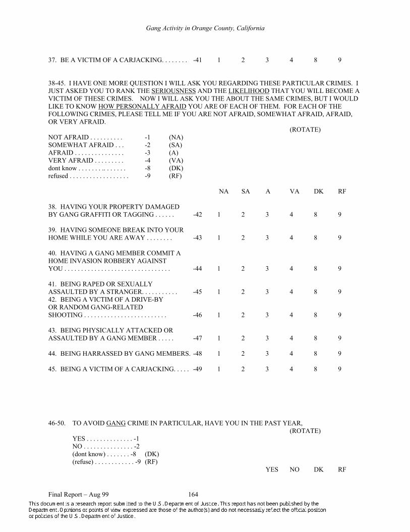
Gang Activity in Orange County, California
37. BE A VICTIM OF A CARJACKING. . . . . . . . -41 1 2 3 4 8 9 38-45. I HAVE ONE MORE QUESTION I WILL ASK YOU REGARDING THESE PARTICULAR CRIMES. I JUST ASKED YOU TO RANK THE SERIOUSNESS AND THE LIKELIHOOD THAT YOU WILL BECOME A VICTIM OF THESE CRIMES. NOW I WILL ASK YOU THE ABOUT THE SAME CRIMES, BUT I WOULD LIKE TO KNOW HOW PERSONALLY AFRAID YOU ARE OF EACH OF THEM. FOR EACH OF THE FOLLOWING CRIMES, PLEASE TELL ME IF YOU ARE NOT AFRAID, SOMEWHAT AFRAID, AFRAID, OR VERY AFRAID.
(ROTATE) NOT AFRAID . . . . . . . . . . -1 (NA) SOMEWHAT AFRAID . . . -2 (SA) AFRAID . . . . . . . . . . . . . . . -3 (A) VERY AFRAID . . . . . . . . . -4 (VA) dont know . . . . . . . .. . . . . . . -8 (DK) refused . . . . . . . . . . . . . . . . . . -9 (RF)
NA SA A VA DK RF 38. HAVING YOUR PROPERTY DAMAGED BY GANG GRAFFITI OR TAGGING . . . . . . -42 1 2 3 4 8 9 39. HAVING SOMEONE BREAK INTO YOUR HOME WHILE YOU ARE AWAY . . . . . . . . -43 1 2 3 4 8 9 40. HAVING A GANG MEMBER COMMIT A HOME INVASION ROBBERY AGAINST YOU . . . . . . . . . . . . . . . . . . . . . . . . . . . . . . . . -44 1 2 3 4 8 9 41. BEING RAPED OR SEXUALLY ASSAULTED BY A STRANGER. . . . . . . . . . . -45 1 2 3 4 8 9 42. BEING A VICTIM OF A DRIVE-BY OR RANDOM GANG-RELATED SHOOTING . . . . . . . . . . . . . . . . . . . . . . . . . -46 1 2 3 4 8 9 43. BEING PHYSICALLY ATTACKED OR ASSAULTED BY A GANG MEMBER . . . . . -47 1 2 3 4 8 9 44. BEING HARRASSED BY GANG MEMBERS. -48 1 2 3 4 8 9 45. BEING A VICTIM OF A CARJACKING. . . . . -49 1 2 3 4 8 9 46-50. TO AVOID GANG CRIME IN PARTICULAR, HAVE YOU IN THE PAST YEAR,
(ROTATE) YES . . . . . . . . . . . . . . -1 NO . . . . . . . . . . . . . . . -2 (dont know) . . . . . . . -8 (DK) (refuse) . . . . . . . . . . . . -9 (RF)
YES NO DK RF
Final Report – Aug 99 164

Gang Activity in Orange County, California
46. BOUGHT OR SECURED A GUN . . . . . . . . . . . . . . . . . . . . . . .. . 50- 1 2 8 9 47. CARRIED A GUN OR OTHER WEAPON WHEN YOU WENT OUT 51- 1 2 8 9 48. ARRANGED TO GO OUT WITH SOMEONE SO YOU WOULD NOTBE ALONE . . . . . . . . . . . . . . . . . . . . . . . . . . . . 52- 1 2 8 9 49. AVOIDED CERTAIN AREAS OF ORANGE COUNTY . . . . . 53- 1 2 8 9 50. AVOIDED CERTAIN AREAS OF YOUR OWN COMMUNITY.. 54- 1 2 8 9 51. DO YOU KNOW THE NAMES OF ANY GANGS OR GANG MEMBERS IN YOUR COMMUNITY?
Yes 55-1 No -2 (dont know) -8 (refused) -9
52. ARE THERE AREAS RIGHT AROUND WHERE YOU LIVE--THAT IS, WITHIN A FEW BLOCKS--
WHERE YOU ARE AFRAID TO WALK ALONE?
Yes (SKIP TO Q. 53) 56-1 No (SKIP TO Q. 54) -2 (dont know) -8 (refused) -9
53. ARE YOU AFRAID THERE BECAUSE OF GANG-RELATED CONCERNS?
Yes 57-1 No -2 (dont know) -8 (refused) -9
54. IN THE PAST TWO TO THREE YEARS, DO YOU FEEL MORE SAFE, NOT AS SAFE, OR ABOUT
THE SAME IN YOUR COMMUNITY?
Safer 58-1 Not as safe -2 About the same -3 (dont know) -8 (refused) -9
55A. IN GENERAL, ARE YOU MORE, LESS, OR EQUALLY AFRAID FOR OTHER PEOPLE LIVING IN
YOUR HOME AS YOU ARE FOR YOURSELF?
MORE AFRAID (SKIP TO 55B) 59-1 LESS AFRAID (SKIP TO 56) -2 EQUALLY AFRAID (SKIP TO 56) -3 (dont know) -8 (refused) -9
Final Report – Aug 99 165

Gang Activity in Orange County, California
55B: ARE YOU MORE AFRAID FOR YOUR YOUR PARENTS, YOUR SPOUSE, YOUR CHILDREN, OR
OTHER PEOPLE UNDER 18 WHO ARE LIVING IN YOUR HOME? (CODE, DONT READ)
parents 60-1 spouse -2 children -3 other under 18 -4 (other) -5 (dont know) -8 (refused) -9
56. ON ANOTHER TOPIC, AT WHAT AGE WOULD YOU CONSIDER SOMEONE NO LONGER A
YOUTH? (CODE, DONT READ)
(61-62) under 16 . . . -01 16 -02 17 -03 18 -04 19 -05 20 -06 21 -07 22 -08 23 -09 24 -10 25 -11 over 25 -12 (dont know) -98 (refused) -99
57. DO YOU THINK GANG MEMBERS ARE MOSTLY UNDER 18, ARE MOSTLY 18 AND OLDER, OR
DO YOU THINK THEY ARE ABOUT HALF AND HALF?
Mostly under 18 63-1 Mostly 18 and older -2 half and half -3 (Dont know) -8 (Refused) -9
58. NOW I WILL ASK YOU A FEW QUESTIONS ABOUT YOUR COMMUNITY IN GENERAL. HOW WOULDYOU DESCRIBE THE PEOPLE WHO LIVE IN YOUR COMMUNITY IN TERMS OF SUCH THINGS AS INCOME, EDUCATION, AND LIFESTYLE? WOULD YOU SAY THEY ARE:
VERY MUCH LIKE YOU 64-1 SOMEWHAT LIKE YOU, OR -2 NOT AT ALL LIKE YOU -3 (dont know) -8
Final Report – Aug 99 166
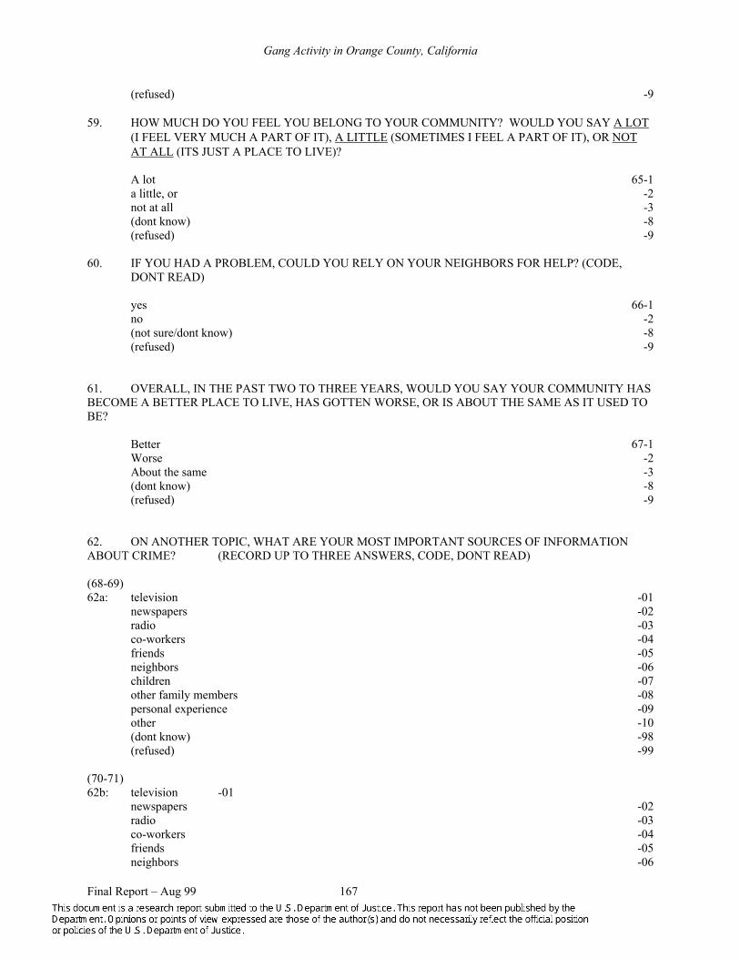
Gang Activity in Orange County, California
(refused) -9 59. HOW MUCH DO YOU FEEL YOU BELONG TO YOUR COMMUNITY? WOULD YOU SAY A LOT
(I FEEL VERY MUCH A PART OF IT), A LITTLE (SOMETIMES I FEEL A PART OF IT), OR NOT AT ALL (ITS JUST A PLACE TO LIVE)?
A lot 65-1 a little, or -2 not at all -3 (dont know) -8 (refused) -9
60. IF YOU HAD A PROBLEM, COULD YOU RELY ON YOUR NEIGHBORS FOR HELP? (CODE,
DONT READ)
yes 66-1 no -2 (not sure/dont know) -8 (refused) -9
61. OVERALL, IN THE PAST TWO TO THREE YEARS, WOULD YOU SAY YOUR COMMUNITY HAS BECOME A BETTER PLACE TO LIVE, HAS GOTTEN WORSE, OR IS ABOUT THE SAME AS IT USED TO BE?
Better 67-1 Worse -2 About the same -3 (dont know) -8 (refused) -9
62. ON ANOTHER TOPIC, WHAT ARE YOUR MOST IMPORTANT SOURCES OF INFORMATION ABOUT CRIME? (RECORD UP TO THREE ANSWERS, CODE, DONT READ) (68-69) 62a: television -01
newspapers -02 radio -03 co-workers -04 friends -05 neighbors -06 children -07 other family members -08 personal experience -09 other -10 (dont know) -98 (refused) -99
(70-71) 62b: television -01
newspapers -02 radio -03 co-workers -04 friends -05 neighbors -06
Final Report – Aug 99 167

Gang Activity in Orange County, California
children -07 other family members -08 personal experience -09 other -10 (dont know) -98 (refused) -99
(72-73) 62c: television -01
newspapers -02 radio -03 co-workers -04 friends -05 neighbors -06 children -07 other family members -08 personal experience -09 other -10 (dont know) -98 (refused) -99
63. ARE YOU A REGULAR VIEWER OF TELEVISION PROGRAMS THAT DEAL WITH CRIME OR
CRIMINAL JUSTICE ISSUES, SUCH AS COPS, REAL STORIES OF THE HIGHWAY PATROL, JUSTICE FILES, OR AMERICAS MOST WANTED? (CODE, DONT READ)
yes 74-1 no -2 (dont know) -3 (refused) -9
64. ON ANOTHER ISSUE, HAVE YOU SEEN OR HEARD ABOUT THE ORANGE COUNTY PROGRAM
DRUG USE IS LIFE ABUSE?
yes (SKIP TO Q. 65) 75-1 no (SKIP TO Q. 67) -2 (dont know) -3 (refused) -9
65. WHERE HAVE YOU SEEN OR HEARD THE SLOGAN DRUG USE IS LIFE ABUSE? (DONT READ,
JUST CODE) (record up to 3 answers) (76-77) 65a. bumper stickers -01
logo in advertising -02 childrens school -03 books, pamphlets -04 newspaper articles, newspaper ads -05 buses -06 bus shelters -07
Final Report – Aug 99 168

Gang Activity in Orange County, California
electronic message board -08 other -09 (dont know) -98 (refused) -99
(78-79) 65b. bumper stickers -01
logo in advertising -02 childrens school -03 books, pamphlets -04 newspaper articles, newspaper ads -05 buses -06 bus shelters -07 electronic message board -08 other -09 (dont know) -98 (refused) -99
(80-81) 65c bumper stickers -01
logo in advertising -02 childrens school -03 books, pamphlets -04 newspaper articles, newspaper ads -05 buses -06 bus shelters -07 electronic message board -08 other -09 (dont know) -98 (refused) -99
66. OVERALL, HOW FAVORABLE AN IMPRESSION DO YOU HAVE OF THE ORGANIZATION AND
THE PROGRAMS INCLUDED IN DRUG USE IS LIFE ABUSE?
VERY FAVORABLE 82-1 SOMEWHAT FAVORABLE -2 SOMEWHAT UNFAVORABLE -3 VERY UNFAVORABLE -4 (dont know) -8 (refused) -9
67-72. TO WHAT DEGREE DO YOU THINK THAT THE FOLLOWING PROBLEMS ARE CAUSED BY
DRUG ABUSE--ON A SCALE OF 1 TO 5 WITH 1 BEING NOT AT ALL AND 5 BEING A LOT? (ROTATE)
NOT LOT DK RF 67. CHILD ABUSE. . . . . . . . . . . . . .. -83 1 2 3 4 5 8 9 68. PROPERTY CRIMES, LIKE BURGLARY
Final Report – Aug 99 169

Gang Activity in Orange County, California
AND THEFT . . . . . . . . . . . . . . . . . . . . . . . -84 1 2 3 4 5 8 9 69. VIOLENT CRIMES, LIKE ASSAULT AND MURDER . . . . . . . . . . . . . . . . . . . . . . . . . . . -85 1 2 3 4 5 8 9 70. VIOLENT CRIMES THAT ARE COMMITTED BY YOUTHS . . . . . . . . . . . . . . . . . . . . . -86 1 2 3 4 5 8 9 71. GANG CRIME . . . . . . . . . . . . . . . . . . -87 1 2 3 4 5 8 9 72. POOR LEARNING ENVIRONMENT IN SCHOOLS . . . . . . . . . . . . . . . . . . . . . . . . . . -88 1 2 3 4 5 8 9 NOW WE WILL ASK YOU A FEW PERSONAL QUESTIONS FOR RESEARCH PURPOSES ONLY. THESE QUESTIONS HELP US UNDERSTAND HOW DIFFERENT PEOPLE IN ORANGE COUNTY FEEL ABOUT THE QUESTIONS WE HAVE ASKED YOU. YOU WILL NOT BE PERSONALLY IDENTIFIED AS HAVING GIVEN THIS INFORMATION. 73. WHAT WAS THE LAST GRADE OF SCHOOL YOU COMPLETED? (CODE, DONT READ)
grade 0-4 89-1 grade 5-8 -2 grade 9-11, some high school -3 grade 12, high school graduate -4 grade 13-15, some college -5 grade 16, college graduate -6 graduate work -7 (dont know) -8 (refused) -9
74. ARE YOU CURRENTLY EMPLOYED FULL-TIME, PART-TIME, OR ARE YOU NOT EMPLOYED?
full-time 90-1 part-time -2 not employed (SKIP TO Q. 76) -3 (dont know) -8 (refused) -9
75. IN YOUR JOB, HOW MUCH CONTACT WOULD YOU SAY YOU HAVE WITH MINORITIES?
WOULD YOU SAY, A LOT, A MODERATE AMOUNT, A SMALL AMOUNT OR NONE? a lot 91-1 a moderate amount -2 a small amount -3 none -4 (dont know) -8 (refused) -9
76. WHAT IS YOUR APPROXIMATE TOTAL HOUSEHOLD YEARLY INCOME? IS IT: (92-93)
LESS THAN $15,000 -01 BETWEEN $15,000 AND $24,999 -02 BETWEEN $25,000 AND $34,999 -03 BETWEEN $35,000 AND $49,999 -04 BETWEEN $50,000 AND $74,999 -05 BETWEEN $75,000 AND $100,000 -06
Final Report – Aug 99 170

Gang Activity in Orange County, California
MORE THAN $100,000 -07 (dont know) -98 (refused) -99
77. ARE YOU MALE OR FEMALE?
male 94-1 female -2 (refused) -9
78. HOW WOULD YOU DESCRIBE YOUR RACE AND ETHNICITY? (CODE, DONT READ)
White/caucasion 95-1 Latino/Hispanic (e.g., Puerto Rican, Mexican, Cuban, Central and South American) -2 African-American/black -3 Asian-American/Pacific Islander (e.g., Filipino, Chinese, Japanese, Hawaiian, Vietnamese) -4 American Indian/Native American -5 Biracial/mixed -6 other -7 (dont know) -8 (refused) -9
79. ARE YOU BETWEEN THE AGES OF:
18 to 20 (96-97)-01 21 to 24 -02 25 to 34 -03 35 to 44 -04 45 to 54 -05 55 to 64 -06 65-74, or -07 75 or older -08 (dont know) -98 (refused) -99
80. WHAT IS YOUR CURRENT MARITAL STATUS? (CODE, DONT READ)
married 98-1 widowed -2 divorced -3 separated -4 never married -5 cohabiting/living with partner -6 (dont know) -8 (refused) -9
81. HOW MANY PEOPLE LIVE IN YOUR HOUSEHOLD? (CODE, DONT READ) (99-100)
1 -01 2 -02 3 -03 4 -04 5 -05 6 -06
Final Report – Aug 99 171

Gang Activity in Orange County, California
7 -07 8 -08 9 -09 10 -10 more than 10 -11 (dont know) -98 (refused) -99
82. HOW MANY PEOPLE LIVING WITH YOU ARE UNDER THE AGE OF 18?
2 -02
(101-102) 0 -00 1 -01
3 -03 4 -04 5 -05 6 -06 7 -07 8 -08 9 -09 10 -10 more than 10 -11 (dont know) -98 (refused) -99
83. DO YOU OWN OR RENT YOUR RESIDENCE?
own 103-1 rent -2 other -3 (dont know) -8 (refused) -9
84. HOW LONG HAVE YOU LIVED IN ORANGE COUNTY?______________
(RECORD EXACT ANSWER)
85. HAVE YOU PERSONALLY BEEN A VICTIM OF A CRIME IN THE PAST TWO TO THREE YEARS?
yes (SKIP TO Q. 86) 104-1 no (SKIP TO Q. 88) -2 (dont know) -8 (refused) -9
86. WAS THIS A VIOLENT CRIME OR A PROPERTY CRIME?
violent 105-1 property -2 both -3 (dont know) -8 (refused) -9
Final Report – Aug 99 172

Gang Activity in Orange County, California
87. DO YOU THINK THIS WAS A GANG-RELATED CRIME?
yes 106-1 no -2 (dont know) -8 (refused) -9
88. HAS ANYONE ELSE IN YOUR FAMILY BEEN A VICTIM OF A CRIME IN THE PAST TWO TO
THREE YEARS?
yes (SKIP TO Q. 89) 107-1 no (SKIP TO Q. 91) -2 (dont know) -8 (refused) -9
89. WAS THIS A VIOLENT CRIME OR A PROPERTY CRIME?
violent 108-1 property -2 both -3 (dont know) -8 (refused) -9
90. DO YOU THINK THIS WAS A GANG-RELATED CRIME?
yes 109-1 no -2 (dont know) -8 (refused) -9
91. FOR RESEARCH PURPOSES ONLY, MAY I HAVE THE CLOSEST CROSS STREETS TO YOUR
HOME?
________________________________ AND ________________________________ 92. WHAT CITY DO YOU LIVE IN?
Final Report – Aug 99 173

Gang Activity in Orange County, California
APPENDIX C. DISSEMINATION OF PROJECT INFORMATION ACTIVITIES
Publications
Vila, Bryan and James W. Meeker (1997) “A Regional Gang Incident Tracking System.” Journal of Gang Research 4:3:23-36.
Meeker, James W. and Bryan Vila. (proposed) Understanding Street Gang Crime.
Doctoral Dissertations
Thomas E. Fossati, Thomas E. 1998. The Social Ecology Of Violent Gang Crime: A Sociospatial Ratiocination. University of California, Irvine.
Lane, Jodi. 1998. Crime and Gangs in an Urban Sphere: Constructing the Threat and Fearing the Future. University of California, Irvine.
Parsons, Katie J.B. 1998. The Gang Incident Tracking System: Orange County, California's Collective Effort to Track Gang-Related Incidents. University of California, Irvine.
Conference Presentations
November 1998: Research team members are scheduled to make five different presentations related to project research at the American Society of Criminology annual meeting.
March 1998: “Relationships Between Concentrations of Gang Incidents, Social and Demographic Factors, and Reported Fear of Gang Crime.” James W. Meeker, Bryan Vila, and Douglas Wiebe, Academy of Criminal Justices Sciences Annual Conference.
February 1998: “Fear of Gangs in Orange County, California.” Jodi Lane, James W. Meeker, and Bryan Vila, Western Society of Criminology.
December 1997: GITS presentation to National Community Oriented Policing Conference, James W. Meeker.
Final Report – Aug 99 174

Gang Activity in Orange County, California
November 1997: “Using a GIS-Based Gang Incident Tracking System to Evaluate Intervention and Violence Reduction Programs.” Bryan Vila and James W. Meeker, American Society of Criminology Annual Conference.
November 1997: “Relationships between Concentration of Gang Incidents, Social and Demographic Factors, and Reported Fear of Gang Crime.” Thomas E. Fossati, James W. Meeker, Bryan Vila.
November 1997: “GIS-Based Mapping of Gang Incidents in Orange County, California.” James W. Meeker and Bryan Vila, American Society of Criminology Annual Conference.
November 1997: “The Gang Incident Tracking System: A Geospatial Analysis of Gang Crime.” Thomas E. Fossati, American Society of Criminology Annual Conference.
November 1997: “If We Don’t Deal with This, We are Going to Have Another LA Problem: The Social Construction of Gang Problems by Law Enforcement and Community Leaders.” Jodi Lane, American Society of Criminology Conference.
November 1997: “Target Type Approaches to Street Gangs: A Preliminary Evaluation of the Effects of Joint Prosecutor, Police, and Probation Teams. American Society of Criminology Annual Meeting.” Douglas Wiebe and James W. Meeker.
July 1997: “A Triangular Approach to Evaluating the Effectiveness of Regional Street Gang Prevention, Intervention, and Suppression Programs.” Bryan Vila and James W. Meeker, U.S. Department of Justice-sponsored Conference on Criminal Justice Research and Evaluation.
March 1997: “Spatial and Temporal Distribution of Gang Crimes.” James W. Meeker, Bryan Vila and Douglas Wiebe, Academy of Criminal Justices Sciences Annual Conference.
March 1997: “The Hourly Distribution of Incidents in Orange County Gang Incident Tracking System Data.” Douglas Wiebe. Academy of Criminal Justice Sciences Annual Meeting
March 1997: “Don’t You Go [Out] There: The Effects of Social Disorganization Variables on Fear of Crime and Gangs.” Jodi Lane, Academy of Criminal Justice Sciences Conference.
November 1996: “Gang Typologies and Criminal Activities.” James W. Meeker and Bryan Vila, American Society of Criminology Annual Conference.
November 1996: “Subcultural Diversity and the Fear of Crime and Gangs.” Jodi Lane, American Society of Criminology Conference.
November 1996: “Temporal and Spatial Analysis of Gang Incidents at the Census Block Level.” Thomas E. Fossati, American Society of Criminology Conference.
Final Report – Aug 99 175

Gang Activity in Orange County, California
June 1996: “Orange County, California’s Regional Gang Incident Tracking System.” Bryan Vila, National Youth Gang Symposium, Dallas, Texas.
May 1996: “Gang Research in Orange County, California.” All Staff, National Institute of Justice & Office of Juvenile Justice and Delinquency Prevention Gangs Cluster Conference.
March 1996: “The Orange County Gang Incident Tracking System.” Bryan Vila, Academy of Criminal Justice Sciences Annual Conference.
March 1996: “An Approach to Understanding Fear of Gangs as a Function of Community Characteristics.” Jodi Lane, Academy of Criminal Justice Sciences Annual Conference.
March 1996: “Spatial Analysis of Gang Crime.” Thomas E. Fossati, Academy of Criminal Justice Sciences Annual Conference.
November 1995: “Regional Variation in Gang-Related Crime Patterns: A Preliminary Analysis of Orange County’s Gang Incident Tracking System.” Bryan Vila and James W. Meeker. American Society of Criminology Annual Conference.
Public Presentations
December 1998: “Gang Turf & Political Turf: Mapping Gang Incidents Across 30 Municipal Boundaries.” Bryan Vila. National Crime Mapping Conference.
November 1998: “Opportunities and Difficulties Associated with Regional Gang Incident Mapping.” James W. Meeker. National Community Oriented Policing Conference.
April 1998: Presentation regarding GITS to San Jose, Calif. Task Force on Gangs, James W. Meeker.
April 1998: Presentation on Orange County Street Gangs and GITS to OJJDP, James W. Meeker and Bryan Vila.
October 1997: “Mapping and Understanding Gang Incidents.” Thomas E. Fossati, University of Wyoming.
August 1997: “GITS and GIS: Usefulness of Tracking Gang Incidents with Geographic Information Software.” Thomas E. Fossati, Orange County Chiefs’ and Sheriff’s Association.
May 1997: Presentation to annual meeting of Orange County Chiefs’ and Sheriff’s Association, Bryan Vila and James W. Meeker.
April 1997: Television interview on OCN re Orange County gangs and GITS, James W. Meeker.
Final Report – Aug 99 176

Gang Activity in Orange County, California
April 1997: “Logistics of Creating Orange County’s Fear of Gangs Survey.” Jodi Lane, the Anti-Gang Initiative Second Cluster Conference, Office of Community Oriented Policing, U.S. Department of Justice.
January 1997: “UCIFRG’S Approach to Measuring Fear of Gangs.” All Staff, National Youth Gang Center Data Collection Focus Group.
September 1996: “Gang Incident Tracking System (GITS).” James W. Meeker, Thomas E. Fossati, Jodi Lane, Katie J.B. Parsons, Orange County Crime Analysts’ Association.
September 1996: “Using GIS and Geographic Modeling to Track Gang Incidents Throughout the County.” Thomas E. Fossati, to Orange Coast Regional Career Criminal Apprehension Program. Training Workshop on GIS Capabilities in Law Enforcement.
September 1996: Presentation to COPS Intensive Case Study Workshop under Anti-Gang Initiative, James W. Meeker.
June 1996: Presentation to Pacific Mutual Foundation Board of Directors, James W. Meeker and Bryan Vila.
June 1996: “Policy Issues Associated with Cross-Jurisdictional Measurement of Gang Incidents.” James W. Meeker and Bryan Vila, FBI Southwest Command College Law Enforcement Executive Development Series.
April 1996: “Measuring Gang Activity in Orange County.” Bryan Vila, UCI Social Ecology Associates lecture series.
February 1996: Presentation to the California Wellness Foundation. Bryan Vila.
Reports Prepared for Local Government Agencies
1996–1998: Annual reports to Orange County Chiefs’ and Sheriff’s Association on gang incident trends (three were prepared).
1996–1998: Individual reports to each of the county’s 22 law enforcement agencies on gang incident trends (three were prepared).
1997: Special report regarding analysis of gang incidents involving drug use or possession
1997: Gang territories maps for City of Westminster
1997–1998: Gang “hot spot” maps countywide and for selected cities
Final Report – Aug 99 177

Gang Activity in Orange County, California
Final Report – Aug 99 178
Reports Prepared for Federal Agencies
Wiebe, Douglas, James W. Meeker, & Bryan Vila. (1998, under review). OJJDP Fact Sheet: Hourly trends of juvenile and adult arrest incidents in 1994-1996. Washington, DC: Office of Juvenile Justice and Delinquency Prevention.
Wiebe, Douglas. (1997). Hourly Juvenile and Adult Arrest Incidents in 1994 and 1995. Irvine, CA: University of California. In Sickmund, Melissa, Snyder, Howard N., & Poe-Yamagata, Eileen. Juvenile Offenders and Victims: 1997 Update on Violence. Washington, DC: Office of Juvenile Justice and Delinquency Prevention.