Games with Strategic Complements and Substitutes

By

Andrew J. Monaco Tarun SabarwalDepartment of Economics Department of EconomicsUniversity of Puget Sound University of KansasTacoma, WA, 98416, USA Lawrence KS, 66045, USAamonaco@pugetsound.edu sabarwal@ku.edu

Abstract

This paper studies games with both strategic substitutes and strategic complements,and more generally, games with strategic heterogeneity (GSH). Such games may behavedifferently from either games with strategic complements or games with strategic sub-stitutes. Under mild assumptions (on one or two players only), the equilibrium set ina GSH is totally unordered (no two equilibria are comparable in the standard productorder). Moreover, under mild assumptions (on one player only), parameterized GSH donot allow decreasing equilibrium selections. In general, this cannot be strengthened toconclude increasing selections. Monotone comparative statics results are presented forgames in which some players exhibit strategic substitutes and others exhibit strategiccomplements. For two-player games with linearly ordered strategy spaces, there is a char-acterization. More generally, there are sufficient conditions. The conditions apply onlyto players exhibiting strategic substitutes; no additional conditions are needed for playerswith strategic complements. Several examples highlight the results.

JEL Numbers: C70, C72Keywords: Lattice games, strategic complements, strategic substitutes, strategic hetero-geneity, equilibrium set, monotone comparative statics

First Draft: April 2010This Version: January 26, 2015

1 Introduction

Games with strategic substitutes (GSS) and games with strategic complements (GSC)

formalize two basic strategic interactions and have widespread applications. In GSC, best

response of each player is weakly increasing in actions of the other players, whereas GSS

have the characteristic that the best response of each player is weakly decreasing in the

actions of the other players.1

This paper focuses on games with both strategic substitutes and strategic comple-

ments. Relatively little is known about such games even though several classes of inter-

actions fall in this category. For example, a classic application in Singh and Vives (1984)

considers a duopoly in which one firm behaves as a Cournot-firm (exhibiting strategic

substitutes) and the other as a Bertrand-firm (with strategic complements). Variations of

the classic matching pennies game provide other examples. A Becker (1968) type game of

crime and law enforcement is another example: the criminal exhibits strategic substitutes

(the greater is law enforcement, the lower is crime) and the police exhibit strategic com-

plements (the greater is crime, the greater is law enforcement). Such games also arise in

studies of pre-commitment in industries with learning effects, see Tombak (2006). More-

over, Fudenberg and Tirole (1984) and Dixit (1987) present examples of pre-commitment

where the strategic property of one player’s action is opposite to that of the other player.

More recent examples are found in Shadmehr and Bernhardt (2011), analyzing collective

1 There is a long literature developing the theory of GSC. Some of this work can be seen in Topkis

(1978), Topkis (1979), Bulow, Geanakoplos, and Klemperer (1985), Lippman, Mamer, and McCardle

(1987), Sobel (1988), Milgrom and Roberts (1990), Vives (1990), Milgrom and Shannon (1994), Mil-

grom and Roberts (1994), Zhou (1994), Shannon (1995), Villas-Boas (1997), Edlin and Shannon (1998),

Echenique (2002), Echenique (2004), Quah (2007), and Quah and Strulovici (2009), among others. Ex-

tensive bibliographies are available in Topkis (1998), in Vives (1999), and in Vives (2005). There is a

growing literature on GSS: confer Amir (1996), Villas-Boas (1997), Amir and Lambson (2000), Schipper

(2003), Zimper (2007), Roy and Sabarwal (2008), Acemoglu and Jensen (2009), Amir, Garcia, and Knauff

(2010), Acemoglu and Jensen (2010), Roy and Sabarwal (2010), Jensen (2010), and Roy and Sabarwal

(2012), among others.

1

actions in citizen protests and revolutions, and Baliga and Sjostrom (2012), analyzing

third-party incentives to manipulate conflict between two players.

Games with both strategic substitutes and strategic complements are the basis for

our more general notion of a game with strategic heterogeneity (GSH), which, in prin-

ciple, allows for arbitrary strategic heterogeneity among players. Moreover, the unified

framework of GSH helps clarify the scope of results found separately for GSC or GSS.

We present three main results.

First, we show that under mild conditions, the equilibrium set in a GSH is totally

unordered (no two equilibria are comparable in the standard product order). These con-

ditions can take one of two forms: either just one player has strictly decreasing and

singleton-valued best response, or one player has strictly decreasing best response and

one player has strictly increasing best response; in either case there are no restrictions on

strategic interactions among other players. Three implications of this result are notable.

Firstly, the nice order and structure properties of the equilibrium set in GSC2 do not sur-

vive a minimal introduction of strategic substitutes, in the sense that if we modify a GSC

so that just one player has strict strategic substitutes3 and has a singleton-valued best

response, then the order structure of the equilibrium set is destroyed completely; no two

equilibria are comparable. Similarly, if we modify a GSC to require that one player has

strict strategic complements,4 and another has strict strategic substitutes, then again the

order structure of the equilibrium set is destroyed completely. Secondly, the non-ordered

nature of equilibria implies that starting from one equilibrium, algorithms to compute

another equilibrium may be made more efficient by discarding two areas of the strategy

2The equilibrium set in a GSC always has a smallest and a largest equilibrium, and more generally,

the equilibrium set is a non-empty, complete lattice. These properties are useful to provide simple and

intuitive algorithms to compute equilibria and to show monotone comparative statics of equilibria in

GSC. In contrast, in GSS, the equilibrium set is totally unordered: no two equilibria are comparable in

the standard product order.3Intuitively, best response is strictly decreasing in other player strategies.4Intuitively, best response is strictly increasing in other player strategies.

2

space. Thirdly, if player strategy spaces are linearly ordered,5 then the set of symmetric

equilibria is non-empty, if, and only if, there is a unique symmetric equilibrium.6 There-

fore, in such cases, there is at most one symmetric equilibrium. In this regard, a game

with both strategic substitutes and strategic complements is different from a GSC and

resembles more the results for a GSS.

Second, we show that under mild conditions, parameterized GSH do not allow decreas-

ing equilibrium selections (as the parameter increases, equilibria do not decrease). These

conditions can take one of two forms: either just one player has strict strategic substitutes

and singleton-valued best response, or just one player has strict strategic substitutes and

strict single-crossing property in (own variable; parameter); in either case, there are no

restrictions on strategic interaction among other players. Recall that in a GSC, (leaving

aside stability issues,) it is possible to find a higher equilibrium at a lower parameter and

a lower equilibrium at a higher parameter. In a GSS, however, there are no decreasing

equilibrium selections. Therefore, our second result implies that decreasing selections in

a GSC are eliminated with a “minimal” introduction of strategic substitutes. Moreover,

an example shows that our second result cannot be strengthened to yield increasing equi-

libria more generally. In this regard, too, a GSH is different from a GSC and more closely

resembles known results for a GSS.

Third, we present monotone comparative statics results (at a higher parameter value,

there are equilibria in which all players take a higher action) for games in which some

players exhibit strategic substitutes and others exhibit strategic complements. For two-

player games in which one player exhibits strategic substitutes, the other player exhibits

strategic complements, and each player has a linearly ordered strategy space, we char-

acterize monotone comparative statics via a condition on the best response of only the

player with strategic substitutes. (No additional condition is imposed on the player with

5As usual, a partially ordered set is linearly ordered, if the partial order is complete; that is, every

two elements are comparable.6As usual, in a symmetric equilibrium, each player plays the same strategy.

3

strategic complements.) The condition is intuitive and is based on a trade-off between

the direct parameter effect and the indirect strategic substitute effect. Notably, the same

condition works for GSS in a similar setting when best responses are singleton-valued.

We present examples to show that this characterization does not hold when there are

more than two players or when strategy spaces are not linearly ordered. For the more

general case, when some players exhibit strategic substitutes and others exhibit strategic

complements, we present sufficient conditions that guarantee monotone comparative stat-

ics. As in the two-player case, these conditions are needed only for players with strategic

substitutes. The conditions are stronger than in the two-player case, but still involve a

trade-off between the direct parameter effect and the indirect strategic substitute effect.

In this regard, games with both strategic substitutes and complements behave differently

from either GSC or GSS.

Recall that if an analyst can choose a new order, then Echenique (2004) shows that

there may exist partial orders in which a strategic game can be viewed as a GSC. This

approach is useful when a partial order is not intrinsic to the game, and its choice does not

materially affect the interpretation of “more” and “less”. The framework in this paper

is more appropriate when there is a natural order on a player’s strategy space and an

interest in equilibrium predictions and comparative statics in this order. For example,

when considering the impact of taxes or subsidies on firm output, a natural order on

output space is the standard order on the real numbers, (and not some other order in

which the game may be viewed as a GSC). In our framework, the order on a player’s

strategy space is considered a fixed primitive of the game.

The paper proceeds as follows. Section 2 defines games with strategic heterogene-

ity and presents the first main result on the structure of the equilibrium set in such

games. Section 3 defines parameterized games with strategic heterogeneity, sub-section

3.1 presents the second main result on non-decreasing equilibrium selections, and sub-

section 3.2 presents the third main result on monotone comparative statics. Section 4

concludes.

4

2 Games with Strategic Heterogeneity

Recall that a lattice is a partially ordered set in which every two elements x and y have a

supremum, denoted x∨ y, and an infimum, denoted x ∧ y. A complete lattice is a lattice

in which every non-empty subset has a supremum and infimum in the set.7 A function

f : X → R (where X is a lattice) is quasi-supermodular if (1) f(x) ≥ f(x ∧ y) =⇒

f(x∨ y) ≥ f(y), and (2) f(x) > f(x∧ y) =⇒ f(x∨ y) > f(y). A function f : X ×T → R

(where X is a lattice and T is a partially ordered set) satisfies single-crossing property

in (x; t) if for every x′ ≺ x′′ and t′ ≺ t′′, (1) f(x′, t′) ≤ f(x′′, t′) =⇒ f(x′, t′′) ≤ f(x′′, t′′),

and (2) f(x′, t′) < f(x′′, t′) =⇒ f(x′, t′′) < f(x′′, t′′).

Consider finitely many players I, and for each player i = 1, . . . , I, a strategy space

that is a partially ordered set, denoted (Xi,�i), and a real-valued payoff function, denoted

ui(xi, x−i). As usual, the domain of each ui is the product of the strategy spaces, (X,�),

endowed with the product order.8 The strategic game Γ ={

(Xi,�i, ui)Ii=1

}

is a game

with strategic heterogeneity, or GSH, if for every player i,

1. Xi is a non-empty, complete lattice, and

2. For every x−i, ui is upper-semicontinuous in xi.9

The definition of a GSH here is very general, allowing for arbitrary heterogeneity

in strategic interaction among the players. In particular, no restriction is placed on

whether players have strategic complements or strategic substitutes. Consequently, this

definition allows for games with strategic complements, games with strategic substitutes,

and mixtures of the two.

For each player i, the best response of player i to x−i is denoted βi(x−i), and is

given by argmaxxi∈Xiui(xi, x−i). As the payoff function is upper-semicontinuous and the

7This paper uses standard lattice terminology. See, for example, Topkis (1998).8For notational convenience, we shall usually drop the index i from the notation for the partial order.9In the standard order interval topology.

5

strategy space is compact in the order interval topology, for every i, and for every x−i,

βi(x−i) is non-empty. Let β : X ։ X , given by β(x) = (βi(x−i))Ii=1, denote the joint

best response correspondence.

As usual, a (pure strategy) Nash equilibrium of the game is a profile of player

actions x such that x ∈ β(x). The equilibrium set of the game is given by E =

{x ∈ X|x ∈ β(x)}. Needless to say, at this level of generality, a GSH may have no Nash

equilibrium. For example, the textbook two-player matching pennies game is admissible

here, and has no pure strategy Nash equilibrium. One may impose additional conditions

to invoke standard results to guarantee existence of equilibrium via Brouwer-Schauder

type theorems, or Kakutani-Glicksberg-Ky Fan type theorems, or other types of results.

For the most part, we do not make these assumptions so that our results apply when-

ever equilibrium exists, regardless of whether a specific equilibrium existence theorem is

invoked, or whether an equilibrium is shown to exist directly in a game. Toward the end

of the paper, in theorems 5 and 6, we make standard assumptions to guarantee existence

of equilibrium; these are used to guarantee existence of a “higher” equilibrium.

Of particular interest to us are cases where the best response of a player is either

increasing (the case of strategic complements) or decreasing (the case of strategic substi-

tutes) with respect to the strategies of the other players. Here, increasing or decreasing

are with respect to an appropriately defined set order, as follows.

Recall that if the payoff function of player i is quasi-supermodular in xi, and satisfies

the single-crossing property in (xi; x−i), then the best response correspondence of player

i is nondecreasing in the induced set order. (The standard induced set order is defined

as follows: for non-empty subsets A,B of a lattice X , A ⊑in B, if for every a ∈ A, and

for every b ∈ B, a ∧ b ∈ A, and a ∨ b ∈ B.) In other words, x′−i � x′′

−i ⇒ βi(x′−i) ⊑in

βi(x′′−i). When player i’s best response is a function, this translates into the standard

definition of a weakly increasing function: x′−i � x′′

−i ⇒ βi(x′−i) � βi(x′′

−i). Let us

formalize this by saying that player i has strategic complements, if player i’s best

6

response correspondence βi is non-decreasing in x−i in the induced set order. A game

with strategic complements, or GSC, is a GSH in which every player i has strategic

complements.

Similarly, in a GSH, if the payoff function of each player i is quasi-supermodular in

xi, and satisfies the dual single-crossing property in (xi; x−i),10 then the best response

correspondence of each player is nonincreasing in the standard induced set order: x′−i �

x′′−i ⇒ βi(x′′

−i) ⊑in βi(x′−i). When player i’s best response is a function, this translates into

the standard definition of a weakly decreasing function: x′−i � x′′

−i ⇒ βi(x′′−i) � βi(x′

−i).

Let us formalize this by saying that player i has strategic substitutes, if player i’s best

response correspondence βi is non-increasing in x−i in the induced set order. A game

with strategic substitutes, or GSS, is a GSH in which every player i has strategic

substitutes.

Notice that the definitions of strategic complements and strategic substitutes are weak

versions, because both admit a best response correspondence that is constant in other

player actions. Therefore, it is useful to define strict versions of these ideas as well.

Consider the following set order. For non-empty subsets A,B of a lattice X , A is strictly

lower than B, denoted A ⊏s B, if for every a ∈ A, and for every b ∈ B, a ≺ b. This

definition is a slight strengthening of the following set order defined in Shannon (1995): A

is completely lower than B, denoted A ⊑c B, if for every a ∈ A, and for every b ∈ B,

a � b. Notice that when A and B are non-empty, complete sub-lattices of X , A is strictly

lower than B, if, and only if, supA ≺ inf B; and similarly, A is completely lower than B,

if, and only if, supA � inf B.

Let us say that player i has quasi-strict strategic complements, if for every

x′−i ≺ x′′

−i, βi(x′

−i) ⊑c βi(x′′

−i). Notice that when best response is singleton-valued, quasi-

10A function f : X×T → R (where X is a lattice and T is a partially ordered set) satisfies dual single-

crossing property in (x; t) if for every x′ ≺ x′′ and t′ ≺ t′′, (1) f(x′′, t′) ≤ f(x′, t′) =⇒ f(x′′, t′′) ≤

f(x′, t′′), and (2) f(x′′, t′) < f(x′, t′) =⇒ f(x′′, t′′) < f(x′, t′′). This is a natural generalization of Amir

(1996).

7

strict strategic complements is equivalent to strategic complements, and therefore, may

not necessarily yield strictly increasing best responses. Say that player i has strict

strategic complements, if for every x′−i ≺ x′′

−i, βit(x

′−i) ⊏s βi

t(x′′−i). In other words,

player i’s best response is increasing in x−i in the strictly lower than set order. Ap-

plying a result due to Shannon (1995) and based on Milgrom and Shannon (1994), if

player i’s payoff is strictly quasi-supermodular in xi,11 and player i’s payoff satisfies strict

single-crossing property in (xi, x−i),12 then player i has quasi-strict strategic complements.

Moreover, in finite-dimensional Euclidean spaces, Edlin and Shannon (1998) provide an

additional intuitive and easy-to-use differentiable condition regarding strictly increasing

marginal returns to derive a comparison in the strictly lower than set order, and therefore,

to conclude that player i has strict strategic complements.

Similarly, player i has quasi-strict strategic substitutes, if for every x′−i ≺ x′′

−i,

βi(x′′−i) ⊑c β

i(x′−i), and player i has strict strategic substitutes, if for every x′

−i ≺

x′′−i, β

it(x

′′−i) ⊏s β

it(x

′−i). The conditions for strict strategic complements and quasi-strict

strategic complements can be easily adapted for substitutes.

Our first result, theorem 1 shows how a single player with (strict) strategic substitutes

can destroy the order structure of the equilibrium set.

Theorem 1. In a GSH, suppose one of the following conditions is satisfied.

1. One player has strict strategic substitutes and singleton-valued best response.

2. One player has strict strategic substitutes and another player has strict strategic

complements.

In either case, if x∗ and x are distinct equilibria, then x∗ and x are not comparable.

11A function f : X → R (where X is a lattice) is strictly quasi-supermodular if for all unordered

x, y, f(x) ≥ f(x ∧ y) =⇒ f(x ∨ y) > f(y).12A function f : X×T → R (whereX is a lattice and T is a partially ordered set) satisfies strict single-

crossing property in (x; t) if for every x′ ≺ x′′ and t′ ≺ t′′, f(x′, t′) ≤ f(x′′, t′) =⇒ f(x′, t′′) < f(x′′, t′′).

8

Proof. Suppose condition (1) is satisfied. Suppose, without loss of generality, that player

1 has strict strategic substitutes with singleton-valued best response, and suppose the

distinct equilibria x and x∗ are comparable, with x ≺ x∗. As case 1, suppose x−1 ≺ x∗−1.

Then x1 = β1(x−1) and x∗1 = β1(x∗

−1), and by strict strategic substitutes, x∗1 ≺ x1,

contradicting x ≺ x∗. For case 2, suppose x−1 = x∗−1 and x1 ≺ x∗

1. Then x1 = β1(x−1) =

β2(x∗−2) = x∗

2, contradicting x1 ≺ x∗1. Thus, x

∗ and x are not comparable.

Suppose condition (2) is satisfied. Suppose, without loss of generality, that player 1

has strict strategic substitutes, player 2 has strict strategic complements, and suppose

the distinct equilibria are comparable, with x ≺ x∗. As case 1, suppose x−1 ≺ x∗−1. Then

x1 ∈ β1(x−1) and x∗1 ∈ β1(x∗

−1), and by strict strategic substitutes, x∗1 ≺ x1, contradicting

x ≺ x∗. As case 2, suppose x1 ≺ x∗1. Then x−2 ≺ x∗

−2. As x2 ∈ β2(x−2) and x∗2 ∈ β2(x∗

−2),

strict strategic complements implies x2 ≺ x∗2, whence x−1 ≺ x∗

−1, and we are in case 1.

Thus, x∗ and x are not comparable.

The economic intuition in this proof is straightforward. When condition (2) is satisfied,

in case 1 in the proof, if opponents of player 1 play higher strategies in the x∗ equilibrium

than in the x equilibrium, then player 1 (with strict strategic substitutes) must be playing

a strictly lower strategy in the x∗ equilibrium than in the x equilibrium, and therefore, the

equilibria are non-comparable. Case 2 essentially says that with x ≺ x∗, player 1 cannot

be playing a higher strategy in the x∗ equilibrium. For if he did, then player 2 (with strict

strategic complements) is playing a higher strategy in the x∗ equilibrium, and therefore,

the opponents of player 1 are playing higher strategies in the x∗ equilibrium, whence

player 1 is playing a strictly lower strategy in the x∗ equilibrium, which is a contradiction.

The intuition behind condition (2) is taken further in condition (1), in the sense that

when the best response of the player with strict strategic substitutes is singleton-valued,

the requirement of a player with strict strategic complements can be dropped. Intuitively,

if x ≺ x∗, then we need only consider the case when opponents of player 1 play higher

strategies; that is, x−1 ≺ x∗−1. For if x−1 = x∗

−1, then by singleton-valued best responses,

9

the best response of player 1 to x−1 is the same as her best response to x∗−1, and thus both

equilibria are the same, which is a contradiction. Condition (1) in theorem 1 formalizes

the intuition that adding one player with strict strategic substitutes completely destroys

the order structure of the equilibrium set.

Notice that Roy and Sabarwal (2008) present a different version of this result, using

(joint) best responses that satisfy a never-increasing property. Their result is designed

for GSS. Their technique cannot be used to prove theorem 1, because the conditions of

theorem 1 allow for cases that are excluded by the assumptions used in their proof.13 In

particular, their result cannot cover the examples in this paper. This is not altogether

surprising, given their focus on GSS. Additionally, the proof here is different; it is more

direct and relies more on economic intuition.

Let us look at some applications of theorem 1.

Example 1 (Matching Pennies: Double-or-Nothing). Consider the following ex-

tension of a standard matching pennies game. Each player has two pennies that they lay

on a table with their hand covering the pennies. Once the pennies are revealed, the out-

comes determine the payoffs as follows. Let’s say that a player goes for double-or-nothing,

if she plays either both heads or both tails, and she does not go for double-or-nothing, if

she plays anything else. If the outcome is (H,H) and (H,H), or (T, T ) and (T, T ), that is,

both players go for double-or-nothing and the pennies match, then player 2 wins $2 from

player 1. If the outcome is (H,H); (T, T ), or (T, T ); (H,H), that is, both player go for

double-or-nothing and the pennies do not match, then player 1 wins $2 from player 2. If

both players put up exactly one H and one T , that is, nobody goes for double-or-nothing,

it is a tie and no money changes hands; and if one player goes for double-or-nothing, that

is, plays either (H,H) or (T, T ), and the other does not, (that is, plays (H, T ) or (T,H),)

13Their result excludes the general class in which all-but-one players have quasi-strict strategic com-

plements, the remaining player has at least two actions, and there are no restrictions on the strategic

interaction with the remaining player. Indeed, their result does not apply even when these properties

only hold locally. Details are provided in appendix A.

10

then the player who goes for double-or-nothing loses and pays $1 to the other player. The

payoffs of this zero-sum game are summarized in figure 1.

(H, H) (T, H) (H, T) (T, T)

(H, H) -2, 2 -1, 1 -1, 1 2, -2

(T, H) 1, -1 0, 0 0, 0 1, -1

(H, T) 1, -1 0, 0 0, 0 1, -1

(T, T) 2, -2 -1, 1 -1, 1 -2, 2

Player 2

Pla

yer

1

Figure 1: Matching Pennies: Double-or-Nothing

Assuming H ≺ T , and with the standard product order, the strategy space of each

player has the order (H,H) ≺ (H, T ) ≺ (T, T ); (H,H) ≺ (T,H) ≺ (T, T ); and (T,H) and

(H, T ) are not comparable. Notice that player 1 has strict strategic substitutes, player 2

has strict strategic complements, and the four Nash equilibria (H, T ;T,H), (H, T ;H, T ),

(T,H ;T,H), and (T,H ;H, T ) are all non-comparable. For a more general version without

necessarily specifying payoffs, consider the next example.

Example 2 (A general two-player, four-point GSH). Consider a GSH with two

players. Player 1’s strategy space is a standard four-point lattice, X1 = {a1, b1, c1, d1},

with b1 and c1 unordered, and a1 = b1∧ c1, and d1 = b1∨ c1, shown graphically in figure 2.

Similarly, X2 = {a2, b2, c2, d2}, also shown graphically in figure 2. Suppose player 1’s best

response correspondence is given as follows: β1(a2) = {d1}, β1(b2) = β1(c2) = {b1, c1}, and

β1(d2) = {a1}, and player 2’s best response correspondence is given as follows: β2(a1) =

{a2}, β2(b1) = β2(c1) = {b2, c2}, and β2(d1) = {d2}. Both are depicted in figure 2. It

is easy to check that this example satisfies condition 2 of theorem 1: player 1 has strict

strategic substitutes, player 2 has strict strategic complements. Consequently, the four

11

Nash equilibria (b1, b2), (b1, c2), (c1, b2), and (c1, c2) are all non-comparable. (Notice that

double-or-nothing matching pennies is a special case of this example.)

a1 b1

c1 d1

a2 b2

c2 d2

X1 X2

BR2(d1)

BR2(b1) = BR

2(c1)

BR2(a1)

BR1(a2)

BR1(d2)

BR1(b2) = BR

1(c2)

Figure 2: A General Two-Player, Four-Point GSH

An example in which condition 1 of theorem 1 is satisfied is presented next.

Example 3 (Cournot Duopoly with Spillovers). Consider two firms, an incumbent

(firm 1) and an entrant (firm 2) competing as Cournot duopolists, producing quantities x1

and x2, respectively. Inverse market demand is given by p = a−b(x1+x2), and firm output

is in [0, 8]. Firm 1’s costs are linear, given by a constant marginal cost c1 > 0. Thus, the

incumbent’s profit is given by π1(x1, x2) = (a− b(x1 + x2))x1 − cx1. As∂2π1

∂x2∂x1

= −b < 0,

firm 1’s best response is decreasing in x2. Indeed, firm 1’s best response is given by

x1 = a−c1−bx2

2b. Suppose there is a one-way spillover from the incumbent to the entrant,

say, in the form of cheaper access to industry-specific talent, or having access to superior

supply chain management at a lower cost, and so on, and this lowers firm 2’s costs. The

spillover may depend on firm 1’s output, and is denoted s(x1). Suppose firm 2’s costs are

given by c2x2s(x1). Its profits are given by π2(x1, x2) = (a − b(x1 + x2))x2 − c2x2s(x1).

Firm 2’s best response is given by x2 =a−c2s(x1)−bx1

2b.

Suppose a = 15, b = 12, c1 = 11, c2 = 3, and the spillover function is s(x1) =

23x31−x2

1−

12x1 + 3. (This spillover function is non-negative and non-monotonic: as firm 1’s output

increases from 0 to 1+√2

2≈ 1.2, the spillover reduces from 3 to a local minimum of about

2.1, and then starts to increase.) In this case, best responses are given by β1(x2) = 4− 12x2,

and β2(x1) = max{6 + x1 + 3x21 − 2x3

1, 0}. Thus, condition 1 in theorem 1 is satisfied. It

12

is easy to check that there are three Nash equilibria: (12, 7), (2, 4), and (4, 0), as shown in

figure 3, and as predicted by theorem 1, these are non-comparable.

2 40

4

8

Output of firm 1 (x1)

Outp

ut

of

firm

2 (x

2)

β1(x2)

β2(x1)

(2, 4)

(0.5, 7)

(4, 0)

Figure 3: Cournot Duopoly with Spillovers

The next two examples document some limits of theorem 1. An extension of the

matching pennies: double-or-nothing example shows that non-comparability of equilibria

may hold sometimes with conditions slightly weaker than one player with strict strate-

gic complements and one player with strict strategic substitutes. The Dove-Hawk-type

example shows that weakening the conditions is not possible in general.

Example 1 (Matching Pennies: Double-or-Nothing, Part 2), continued. Con-

sider the following modification to the game of double-or-nothing matching pennies. If

both players go for double-or-nothing and the pennies match (that is, the outcome is

(H,H) and (H,H), or (T, T ) and (T, T )), player 2 wins $2 from player 1, and if both

pennies do not match (the outcome is (H,H); (T, T ), or (T, T ); (H,H)), player 1 wins

13

$2 from player 2. In all other cases, the game is a tie, and no money changes hands.

The payoffs of this zero-sum game are summarized in Figure 4. Assume the same order

structure as in double-or-nothing matching pennies. Notice that player 1 has quasi-strict

strategic substitutes, player 2 has quasi-strict strategic complements, and the four Nash

equilibria are all non-comparable.

(H, H) (T, H) (H, T) (T, T)

(H, H) -2, 2 0, 0 0, 0 2, -2

(T, H) 0, 0 0, 0 0, 0 0, 0

(H, T) 0, 0 0, 0 0, 0 0, 0

(T, T) 2, -2 0, 0 0, 0 -2, 2

Player 2

Pla

yer

1

Figure 4: Matching Pennies: Double-or-Nothing, Part 2

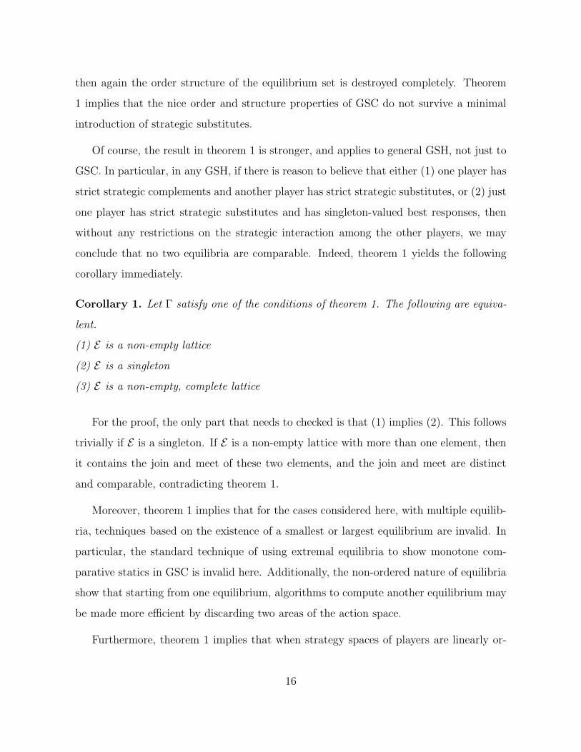
Example 4 (A Dove-Hawk-type game). Consider the GSH with two players given

in figure 5, where for player 1, L ≺ M ≺ H , and for player 2, L ≺ M . We may interpret

L as a low (most Dovish, least Hawkish) action, M as a medium (less Dovish, more

Hawkish) action, and H as a high (or least Dovish, most Hawkish) action. Player 1 has

strict strategic subsitutes, with non-singleton-valued best response: β1(L) = {M,H},

and β1(M) = {L}. Player 2 is of a type that prefers less conflict (or avoids agression, or

would prefer a more “cooperative” action). Player 2 exhibits strategic complements; in

fact, player 2’s best response function is constant, β2(L) = β2(M) = β2(H) = {L}. This

game has two Nash equilibria, (M,L) and (H,L), and these equilibria are comparable,

with (M,L) ≺ (H,L).

Theorem 1 can be used to highlight a particular non-robustness in the order structure

of the equilibrium set in games with strategic complements. Recall that in GSC, the

14

L M

L 0, 5 5, 0

M 5, 5 0, 0

H 5, 5 0, 0

Player 2

Pla

yer

1

Figure 5: A Dove-Hawk-type Game

equilibrium set is a non-empty, complete lattice (see Zhou (1994)), and there exist a

smallest equilibrium and a largest equilibrium (various versions of this result can be seen

in Topkis (1978), Topkis (1979), Lippman, Mamer, and McCardle (1987), Sobel (1988),

Milgrom and Roberts (1990), Vives (1990), Milgrom and Shannon (1994), among others).

On the other hand, in GSS, the equilibrium set is completely unordered: no two equilibria

are comparable (in the standard product order), as shown in Roy and Sabarwal (2008).

Therefore, when we move from a setting in which all players exhibit strategic complements

to a setting in which all players exhibit strategic substitutes, the order structure of the

equilibrium set is destroyed completely.

Theorem 1 can be used to inquire when and by how much the order structure of the

equilibrium set is affected as we move player-by-player from a setting of all players with

strategic complements to a setting of all players with strategic substitutes. Consider a

GSC. In this case, the equilibrium set is a non-empty, complete lattice, and every pair

of equilibria has a smallest larger equilibrium, and a largest smaller equilibrium. If we

modify this game to require that just one player has strict strategic substitutes, and that

player’s best response is singleton-valued (perhaps because that payoff function is strictly

quasi-concave), then the order structure of the equilibrium set is destroyed completely.

That is, no two equilibria are comparable. Similarly, if we modify this game to require that

one player has strict strategic complements, and another has strict strategic substitutes,

15

then again the order structure of the equilibrium set is destroyed completely. Theorem

1 implies that the nice order and structure properties of GSC do not survive a minimal

introduction of strategic substitutes.

Of course, the result in theorem 1 is stronger, and applies to general GSH, not just to

GSC. In particular, in any GSH, if there is reason to believe that either (1) one player has

strict strategic complements and another player has strict strategic substitutes, or (2) just

one player has strict strategic substitutes and has singleton-valued best responses, then

without any restrictions on the strategic interaction among the other players, we may

conclude that no two equilibria are comparable. Indeed, theorem 1 yields the following

corollary immediately.

Corollary 1. Let Γ satisfy one of the conditions of theorem 1. The following are equiva-

lent.

(1) E is a non-empty lattice

(2) E is a singleton

(3) E is a non-empty, complete lattice

For the proof, the only part that needs to checked is that (1) implies (2). This follows

trivially if E is a singleton. If E is a non-empty lattice with more than one element, then

it contains the join and meet of these two elements, and the join and meet are distinct

and comparable, contradicting theorem 1.

Moreover, theorem 1 implies that for the cases considered here, with multiple equilib-

ria, techniques based on the existence of a smallest or largest equilibrium are invalid. In

particular, the standard technique of using extremal equilibria to show monotone com-

parative statics in GSC is invalid here. Additionally, the non-ordered nature of equilibria

show that starting from one equilibrium, algorithms to compute another equilibrium may

be made more efficient by discarding two areas of the action space.

Furthermore, theorem 1 implies that when strategy spaces of players are linearly or-

16

dered,14 the game has at most one symmetric equilibrium. Here, an equilibrium is sym-

metric, if every player plays the same strategy in equilibrium.

Corollary 2. Let Γ satisfy one of the conditions of theorem 1, and suppose the strategy

space of each player is linearly ordered.

The set of symmetric equilibria is non-empty, if, and only if, there is a unique symmetric

equilibrium.

The “only if” direction is proved by noting that with linearly ordered strategy spaces, if

there are two (or more) symmetric equilibria, they are comparable, contradicting theorem

1.

Notice that the definition of symmetric equilibrium here makes no reference to payoffs.

Sometimes, a symmetric equilibrium is considered in games in which (perhaps ex-ante)

payoffs of all players are identical. In that case, each player’s best response is identical to

that of the other players, and for theorem 1 to be applicable, each player would have a

decreasing best response, and the game would necessarily be one of strategic substitutes.

The result here applies to more general situations and allows for strategic heterogeneity.

As a simple class of examples, consider a simple two-player game in which player 1’s payoff

is given by u1(x1, x2) = −x1x2 + kx1, for some positive constant k, and player 2’s payoff

is given by u2(x1, x2) = x1x2. In this case, player 1 has strategic substitutes, player 2 has

strategic complements, and the unique symmetric equilibrium is given by (k, k).

3 Parameterized GSH

Consider finitely many players, I, and for each player i, a strategy space that is a partially

ordered set, denoted (Xi,�i), a real-valued payoff function, denoted ui(xi, x−i, t), and a

partially ordered set of parameters, T . As usual, the product of the strategy spaces,

14As usual, linearly ordered means that every pair of strategies is comparable. A linear order is

sometimes termed a complete order.

17

denoted (X,�), is endowed with the product order and topology. The strategic game

Γ ={

(Xi,�i, ui)Ii=1, T

}

is a parameterized game with strategic heterogeneity, or

parameterized GSH, if for every player i,

1. Xi is a non-empty, complete lattice, and

2. For every (x−i, t), ui is quasi-supermodular and upper-semicontinuous in xi,15 and

3. For every x−i, ui satisfies single-crossing property in (xi; t).

As earlier, for each t ∈ T , and for each player i, the best response of player i to

x−i is denoted βit(x−i), and is given by argmaxxi∈Xi

ui(xi, x−i, t). As the payoff function is

quasi-supermodular and upper-semicontinuous, and the strategy space is compact in the

order interval topology, for every i, and for every (x−i, t), βit(x−i) is a non-empty, complete

sub-lattice. When convenient, we use βi

t(xi) = sup βi

t(xi), and βi

t(x

i) = inf βi

t(xi).

Moreover, as usual, single-crossing property in (xi; t) formalizes the standard idea that

the parameter is complementary to xi. It implies that βit(x−i) is non-decreasing in t in

the induced set order: for every t � t and for every x−i, βit(x−i) ⊑in βi

t(x−i). For each

t ∈ T , let βt : X ։ X given by βt(x) = (βit(x−i))

Ii=1 denote the joint best response

correspondence. From properties of player best responses, it follows that for every

t � t and for every x, βt(x) ⊑in βt(x). As usual, for each t ∈ T , a (pure strategy) Nash

equilibrium is a profile of player actions x such that x ∈ βt(x), and the equilibrium

set at t is given by E(t) = {x ∈ X|x ∈ βt(x)}.

As earlier, say that player i has strategic complements, if for every t, player i’s

best response correspondence βit is non-decreasing in x−i in the induced set order: for

every t and every x′−i � x′′

−i, βit(x

′−i) ⊑in βi

t(x′′−i). Similarly, player i has strategic

substitutes, if for every t, player i’s best response correspondence βit is non-increasing in

x−i in the induced set order: for every t and every x′−i � x′′

−i, βit(x

′′−i) ⊑in βi

t(x′−i). Strict

15In the standard order interval topology.

18

versions are defined similarly. Let us say that player i has quasi-strict strategic

complements, if for every t, and every x′−i ≺ x′′

−i, βit(x

′−i) ⊑c βi

t(x′′−i). Player i has

strict strategic complements, if for every t, and every x′−i ≺ x′′

−i, βit(x

′−i) ⊏s β

it(x

′′−i).

Similarly, player i has quasi-strict strategic substitutes, if for every t, and every

x′−i ≺ x′′

−i, βit(x

′′−i) ⊑c β

it(x

′−i). Moreover, player i has strict strategic substitutes,

if for every t, and every x′−i ≺ x′′

−i, βit(x

′′−i) ⊏s β

it(x

′−i). These properties may be derived

from the same conditions on payoff functions presented earlier.

3.1 Non-Decreasing Equilibrium Selections

The following result shows that in a broad class of parameterized GSH, there are no

decreasing selections of equilibria.

Theorem 2. In a parameterized GSH, suppose one of the following conditions is satisfied.

1. One player has strict strategic substitutes and singleton-valued best response.

2. One player, say player i, has strict strategic substitutes and strict single-crossing

property in (xi; t).

Then for every t∗ ≺ t, for every x∗ ∈ E(t∗), and for every x ∈ E(t), x 6≺ x∗.

Proof. Consider condition 1, and without loss of generality, suppose it is satisfied for

player 1. Suppose x ≺ x∗. As case 1, consider x−1 ≺ x∗−1. Then x∗

1 = β1t∗(x

∗−1) ≺

β1t∗(x−1) � β1

t(x−1) = x1, contradicting x ≺ x∗. Here, the strict inequality follows from

strict strategic substitutes, and the weak inequality follows from single-crossing property

in (x1; t). As case 2, consider x−1 = x∗−1 and x1 ≺ x∗

1. Then x∗1 = β1

t∗(x∗−1) = β1

t∗(x−1) �

β1t(x−1) = x1, contradicting x1 ≺ x∗

1.

Consider condition 2, suppose it is satisfied for player 1, and suppose x ≺ x∗. As case 1,

consider x−1 ≺ x∗−1. Then β1

t∗(x∗−1) ⊏s β

1t∗(x−1) ⊑c β

1t(x−1), where the strictly lower than

19

relation follows from strict strategic substitutes, and the completely lower than relation

follows from strict single-crossing property in (x1; t). Consequently, x∗1 � sup β1

t∗(x∗−1) ≺

inf β1t∗(x−1) � inf β1

t(x−1) � x1, contradicting x1 ≺ x∗

1. As case 2, consider x−1 =

x∗−1 and x1 ≺ x∗

1. Then β1t∗(x

∗−1) = β1

t∗(x−1) ⊑c β1t(x−1), whence x∗

1 � sup β1t∗(x

∗−1) =

sup β1t∗(x−1) � inf β1

t(x−1) � x1, contradicting x1 ≺ x∗

1.

This theorem presents conditions on one player only to derive equilibrium selection

results. In particular, if one player exhibits strict strategic substitutes and has a singleton-

valued best response, then without any restrictions on the strategic interdependence

among the other players, there are no decreasing selections of equilibria. In particu-

lar, this theorem does not require other players to exhibit either strategic substitutes or

strategic complements.

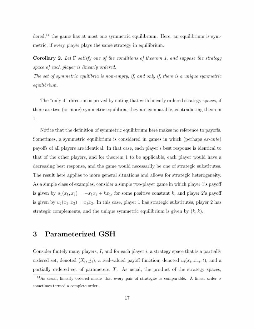
Example 3 (Cournot Duopoly with Spillovers), continued. Recall the best re-

sponses in the Cournot duopoly with spillovers example above, β1(x2) = a−bx2−c12b

, and

β2(x1) =a−bx1−c2s(x1)

2b, and the spillover function, s(x1) =

23x31−x2

1−x1

2+3, and consider a

as the parameter. This game satisfies condition 1 (and 2) in theorem 2. Given parameter

values a = 15, b = 12, c1 = 11, c2 = 3, it is easy to check that there are three Nash

equilibria: (12, 7), (2, 4), and (4, 0), shown in figure 6. If we increase parameter a to 17,

both best responses increase, and there are 3 new equilibria: (1, 10), (1.686, 8.627), and

(6, 0). Notice that no new equilibrium is lower than any old equilibrium, as predicted by

theorem 2. Moreover, firm 1’s output in x∗ = (1.686, 8.627) is lower than its output in

x∗ = (2, 4), showing that in general, we cannot strengthen the conclusion of this theorem

to guarantee increasing equilibria.

Theorem 2 shows that in the presence of strategic substitutes, there are no decreasing

equilibrium selections. Moreover, the example shows that in general, this result cannot

be strengthened to conclude monotone comparative statics. That is, when a parameter

increases, it is possible that there are some higher equilibria, but it is also possible that

there are equilibria that are not higher. Conditions yielding monotone comparative statics

20

9 2 4 6 8

12

0

4

8

x1

x2

β1(x2)

β2(x1)

Figure 6: Non-Decreasing Equilibria For Cournot Duopoly With Spillovers

are considered next.

3.2 Monotone Comparative Statics

Let’s first consider two-player GSH in which one player exhibits strategic substitutes and

the other one exhibits strategic complements. In this setting, we present some results

characterizing monotone comparative statics.

Theorem 3. Consider a two-player, parameterized GSH, in which player 1 has strategic

substitutes, and player 2 has strategic complements. Suppose strategy spaces are linearly

ordered and best responses are singleton-valued.

For every t∗ � t, for every x∗ ∈ E(t∗), and for every x ∈ E(t),

1. x∗2 � x2

2. x∗ � x ⇐⇒ x∗1 � β1

t◦ β2

t(x∗

1)

21

Proof. Consider statement 1. As case 1, suppose x∗1 � x1. Then x∗

2 = β2t∗(x

∗1) � β2

t∗(x1) �

β2t(x1) = x2, where the first inequality follows from strategic complements, and the second

from single-crossing property. As case 2, consider x∗1 6� x1. Linearly ordered strategies

implies x1 ≺ x∗1. In this case, x2 6≺ x∗

2. (For if x2 ≺ x∗2, then x∗

1 = β1t∗(x

∗2) � β1

t(x∗

2) �

β1t(x2) = x1, where, the first inequality follows from single-crossing property and the

second from strategic substitutes. This contradicts x1 ≺ x∗1.) Linearly ordered strategies

now yields x∗2 � x2.

Consider statement 2. For sufficiency, suppose x∗ � x. Then x∗1 � x1, and strategic

complements implies β2t(x∗

1) � β2t(x1), whence x∗

1 � x1 = β1t(β2

t(x1)) � β1

t(β2

t(x∗

1)), where

the inequality follows from strategic substitutes. For necessity, suppose x∗ 6� x. Then,

using statement 1, x∗1 6� x1, and linear order implies x1 ≺ x∗

1. Thus, x2 = β2t(x1) � β2

t(x∗

1),

where the inequality follows from strategic complements. Now, using strategic substitutes

yields β1t(β2

t(x∗

1)) � β1t(x2) = x1 ≺ x∗

1, as desired.

This result formalizes the intuition that in a two-player GSH, when the parameter

(weakly) increases, the equilibrium response of the player with strategic complements is

always (weakly) higher. For monotone comparative statics, we also need the equilibrium

response of the player with strategic substitutes to be (weakly) higher; this is characterized

by the second condition. That is, x∗1 � x1 is equivalent to x∗

1 � β1t◦ β2

t(x∗

1).

The condition x∗1 � β1

t◦ β2

t(x∗

1) can be viewed as follows. Starting from an existing

equilibrium strategy for player 1, x∗1 at t = t∗, an increase in t has two effects on β1

(·)(·).

One effect is an increase in β1, because best response is nondecreasing in t. (This is

the direct effect of an increase in t, arising from the single-crossing property in (x1; t).)

The other effect is a decrease in β1, because an increase in t increases β2t (x

∗1), and β1

is decreasing in x2, due to strategic substitutes. (This is the indirect effect arising from

player 1’s response to player 2’s response to an increase in t.) The condition says that for

player 1, as long as the indirect strategic substitute effect does not dominate the direct

parameter effect, the new equilibrium response of player 1 is (weakly) larger than x∗1. This

22

can be viewed explicitly in the following example.

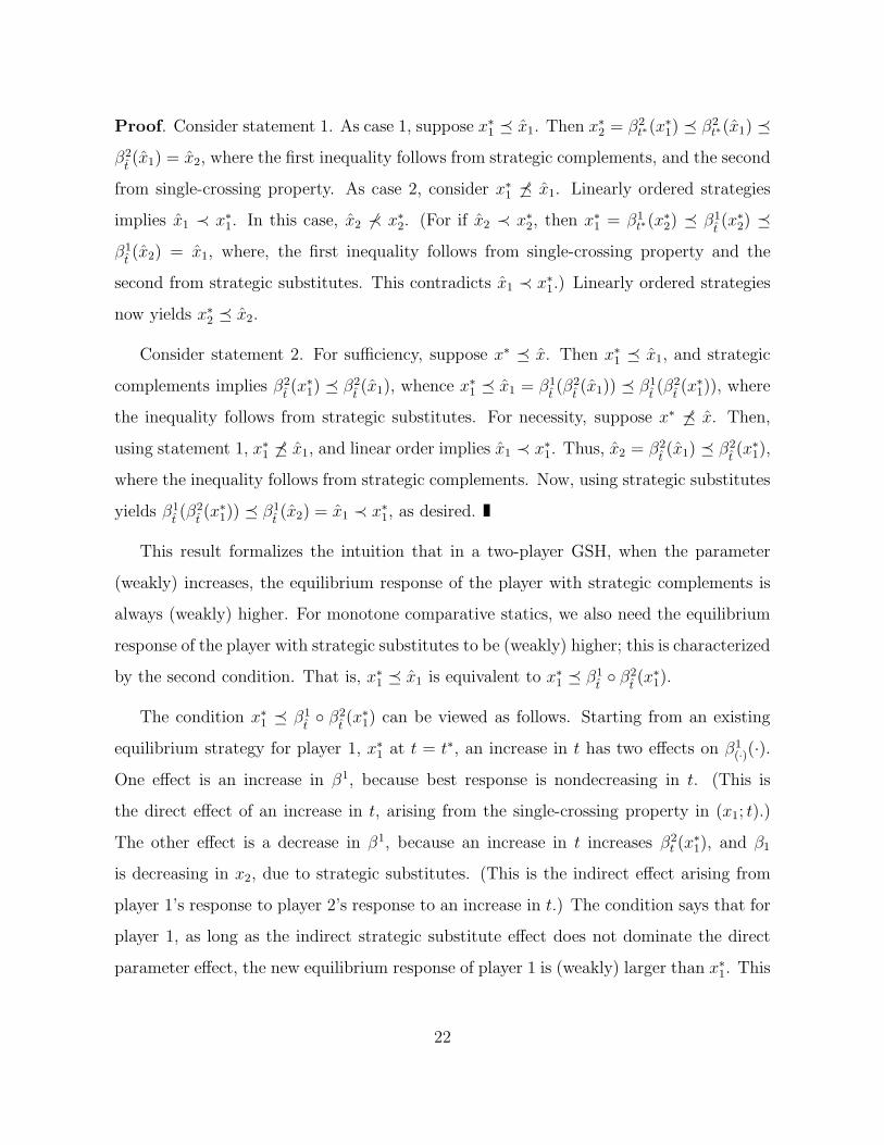
Example 5 (Differentiated Duopoly). Consider the differentiated duopoly in Singh

and Vives (1984), where firm 1 chooses price as a strategic variable, and firm 2 chooses

quantity. Inverse market demand for each firm is given by p1 = a1−b1q1−cq2 and p2 = a2−

cq1 − b2q2.16 We may view the demand parameters (a1, a2) as the parameter of the game.

Re-writing firm 1’s demand yields q1(p1, q2) =1b1(a1 − cq2 − p1), and assuming zero cost,

firm 1’s profit is π1(p1, q2) = p1q1(p1, q2). Similarly, using firm 1’s demand, and assuming

zero cost, we may write firm 2’s profit as π2(p1, q2) =(

a2 −cb1(a1 − cq2 − p1)− b2q2

)

q2.

It is easy to check that ∂2π1

∂q2∂p1= − c

b1< 0 and ∂2π2

∂q2∂p1= c

b1> 0. In other words, firm 1’s best

response is decreasing in firm 2’s quantity choice, and firm 2’s best response is increasing

in firm 1’s price choice. Indeed, (the linear) best responses are given as follows: for firm

1, p1 =a1−cq2

2, and for firm 2, q2 =

a2b1−a1c+cp12(b1b2−c2)

. Notice that assuming a1 = a2, both best

responses are increasing in the parameter.

Let t = a1 = a2, and rewrite best responses as follows: for firm 1, β1t (q2) =

t−cq22

, and

for firm 2, β2t (p1) =

tb1−tc+cp12(b1b2−c2)

, and notice that best response of both players is increasing in

t. Suppose t = 2, b1 = b2 = 2, and c = 1. In this case, the unique Nash equilibrium is given

by (p∗1, q∗2) = (2

3, 25). Consider an increase to t = 3. In this case, β1

t(β2

t(p∗1)) =

4336

> 23= p∗1,

and therefore, the new equilibrium is higher than the old equilibrium, as shown in figure

7. Indeed, the new equilibrium is (p1, q2) ≈ (1.15, 0.69). (For reference, profits of both

firms have gone up as well, from (0.31, 0.29) to (0.39, 0.72).)

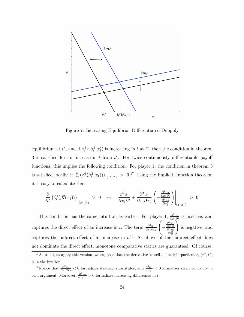
For completeness, figure 8 represents graphically the case where the direct effect does

not dominate the indirect effect. If best responses change in the manner shown in figure

8, the composite effect is lower, (β1t(β2

t(p∗1)) < p∗1,) and as theorem 3 predicts, the new

equilibrium is not higher than the old equilibrium.

When payoff functions are twice continuously differentiable as well, the condition in

theorem 3 can be translated to payoff functions, as follows. Notice that if x∗ is an

16As usual, we assume that a1, a2, b1, b2, c > 0, b1 > c, and b1b2 − c2 > 0.

23

p1

q2

β1(q2)

β2(p1)

p1* β

t

1(βt2(p

1*))ˆ ˆ

Figure 7: Increasing Equilibria: Differentiated Duopoly

equilibrium at t∗, and if β1t ◦ β

2t (x

∗1) is increasing in t at t∗, then the condition in theorem

3 is satisfied for an increase in t from t∗. For twice continuously differentiable payoff

functions, this implies the following condition. For player 1, the condition in theorem 3

is satisfied locally, if ∂∂t(β1

t (β2t (x1)))

∣

∣

(x∗,t∗)> 0.17 Using the Implicit Function theorem,

it is easy to calculate that

∂

∂t

(

β1t (β

2t (x1))

)

∣

∣

∣

∣

(x∗,t∗)

> 0 ⇔∂2u1

∂x1∂t+

∂2u1

∂x1∂x2

(

−∂2u2

∂x2∂t

∂2u2

∂x2

2

)∣

∣

∣

∣

∣

(x∗,t∗)

> 0.

This condition has the same intuition as earlier. For player 1, ∂2u1

∂x1∂tis positive, and

captures the direct effect of an increase in t. The term ∂2u1

∂x1∂x2

(

−∂2u2

∂x2∂t

∂2u2

∂x22

)

is negative, and

captures the indirect effect of an increase in t.18 As above, if the indirect effect does

not dominate the direct effect, monotone comparative statics are guaranteed. Of course,

17As usual, to apply this version, we suppose that the derivative is well-defined; in particular, (x∗, t∗)

is in the interior.18Notice that ∂2u1

∂x1∂x2

< 0 formalizes strategic substitutes, and ∂2u2

∂x2

2

< 0 formalizes strict concavity in

own argument. Moreover, ∂2u2

∂x2∂t> 0 formalizes increasing differences in t.

24

p1

q2

β1(q2)

β2(p1)

p1*β

t

1(βt

2(p1*))

ˆ ˆ

Figure 8: Non-increasing Equilibria: Differentiated Duopoly

theorem 3 holds without differentiability or concavity, and without restriction to convex

strategy spaces.

In order to characterize increasing equilibria with best response correspondences, we

have the following result (which is proved using the three lemmas in Appendix B).

Theorem 4. Consider a two-player, parameterized GSH, in which player 1 has strict

strategic substitutes, and player 2 has strict strategic complements. Suppose strategy spaces

are linearly ordered.

For every t∗ � t, for every x∗ ∈ E(t∗), and for every x ∈ E(t),

1. x∗2 � x2

2. x∗ � x ⇐⇒ x∗1 � β

1

t ◦ β2

t(x∗

1)

Theorems 3 and 4 present results for two-player GSH with linearly ordered strategy

spaces. These results may not necessarily hold more generally, either with non-linearly

ordered strategy spaces, or with more than two players, as shown in the next two examples.

25

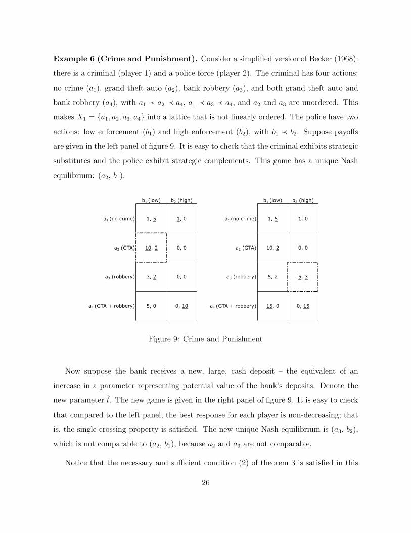
Example 6 (Crime and Punishment). Consider a simplified version of Becker (1968):

there is a criminal (player 1) and a police force (player 2). The criminal has four actions:

no crime (a1), grand theft auto (a2), bank robbery (a3), and both grand theft auto and

bank robbery (a4), with a1 ≺ a2 ≺ a4, a1 ≺ a3 ≺ a4, and a2 and a3 are unordered. This

makes X1 = {a1, a2, a3, a4} into a lattice that is not linearly ordered. The police have two

actions: low enforcement (b1) and high enforcement (b2), with b1 ≺ b2. Suppose payoffs

are given in the left panel of figure 9. It is easy to check that the criminal exhibits strategic

substitutes and the police exhibit strategic complements. This game has a unique Nash

equilibrium: (a2, b1).

b1 (low) b2 (high) b1 (low) b2 (high)

a1 (no crime) 1, 5 1, 0 a1 (no crime) 1, 5 1, 0

a2 (GTA) 10, 2 0, 0 a2 (GTA) 10, 2 0, 0

a3 (robbery) 3, 2 0, 0 a3 (robbery) 5, 2 5, 3

a4 (GTA + robbery) 5, 0 0, 10 a4 (GTA + robbery) 15, 0 0, 15

Figure 9: Crime and Punishment

Now suppose the bank receives a new, large, cash deposit – the equivalent of an

increase in a parameter representing potential value of the bank’s deposits. Denote the

new parameter t. The new game is given in the right panel of figure 9. It is easy to check

that compared to the left panel, the best response for each player is non-decreasing; that

is, the single-crossing property is satisfied. The new unique Nash equilibrium is (a3, b2),

which is not comparable to (a2, b1), because a2 and a3 are not comparable.

Notice that the necessary and sufficient condition (2) of theorem 3 is satisfied in this

26

case, because a2 ≺ a4 = β1t(β2

t(a2)). This example shows that when we extend the analysis

to non-linearly ordered lattices, the analogue of theorem 3 does not necessarily hold.

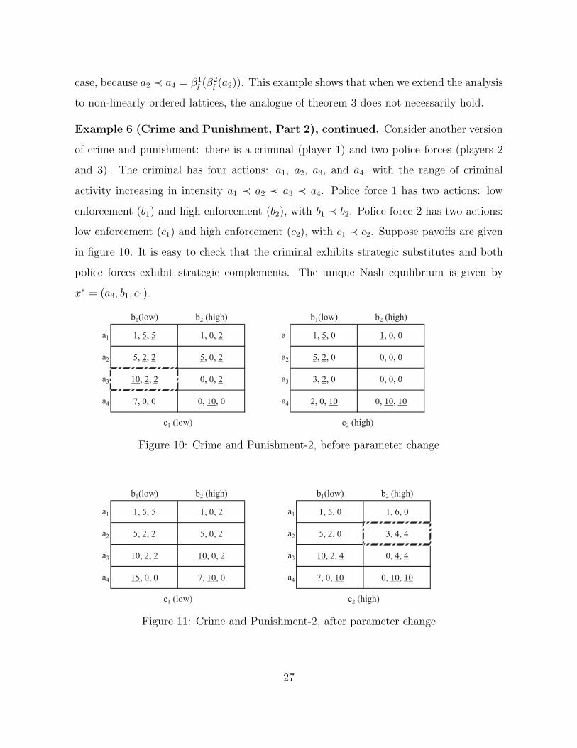
Example 6 (Crime and Punishment, Part 2), continued. Consider another version

of crime and punishment: there is a criminal (player 1) and two police forces (players 2

and 3). The criminal has four actions: a1, a2, a3, and a4, with the range of criminal

activity increasing in intensity a1 ≺ a2 ≺ a3 ≺ a4. Police force 1 has two actions: low

enforcement (b1) and high enforcement (b2), with b1 ≺ b2. Police force 2 has two actions:

low enforcement (c1) and high enforcement (c2), with c1 ≺ c2. Suppose payoffs are given

in figure 10. It is easy to check that the criminal exhibits strategic substitutes and both

police forces exhibit strategic complements. The unique Nash equilibrium is given by

x∗ = (a3, b1, c1).

b1(low) b2 (high) b1(low) b2 (high)

a1 1, 5, 5 1, 0, 2 a1 1, 5, 0 1, 0, 0

a2 5, 2, 2 5, 0, 2 a2 5, 2, 0 0, 0, 0

a3 10, 2, 2 0, 0, 2 a3 3, 2, 0 0, 0, 0

a4 7, 0, 0 0, 10, 0 a4 2, 0, 10 0, 10, 10

c1 (low) c2 (high)

Figure 10: Crime and Punishment-2, before parameter change

b1(low) b2 (high) b1(low) b2 (high)

a1 1, 5, 5 1, 0, 2 a1 1, 5, 0 1, 6, 0

a2 5, 2, 2 5, 0, 2 a2 5, 2, 0 3, 4, 4

a3 10, 2, 2 10, 0, 2 a3 10, 2, 4 0, 4, 4

a4 15, 0, 0 7, 10, 0 a4 7, 0, 10 0, 10, 10

c1 (low) c2 (high)

Figure 11: Crime and Punishment-2, after parameter change

27

Suppose, as earlier, an increase in the parameter corresponds to an increase in the

value of criminal activity to the criminal. Denote the new parameter t, and suppose the

new payoffs are given in figure 11. The unique Nash equilibrium is given by x = (a2, b2, c2),

and this is not comparable to x∗ = (a3, b1, c1).

Notice that the second iterate condition from theorem 3 would be as follows: x∗1 �

β1t(β2

t(x∗

−2), β3t(x∗

−3)). This condition is satisfied, because β2t(a3, c1) = b1, β

3t(a3, b1) = c2,

and therefore, x∗1 = a3 � a3 = β1

t(b1, c2) = β1

t(β2

t(x∗

−2), β3t(x∗

−3)).

Moreover, in the absence of linearly ordered spaces, it is not necessary that the equi-

librium outcome of the player with strategic complements goes up, as shown in the next

example.

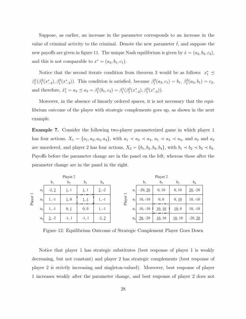
Example 7. Consider the following two-player parameterized game in which player 1

has four actions, X1 = {a1, a2, a3, a4}, with a1 ≺ a2 ≺ a4, a1 ≺ a3 ≺ a4, and a2 and a3

are unordered, and player 2 has four actions, X2 = {b1, b2, b3, b4}, with b1 ≺ b2 ≺ b3 ≺ b4.

Payoffs before the parameter change are in the panel on the left, whereas those after the

parameter change are in the panel in the right.

b1 b2 b3 b4 b1 b2 b3 b4

a1 -2, 2 1, 1 1, 1 2, -2 a1 -20, 20 0, 10 0, 10 20, -20

a2 1, -1 1, 0 1, 1 1, -1 a2 10, -10 0, 0 0, 10 10, -10

a3 1, -1 0, 1 0, 0 1, -1 a3 10, -10 10, 10 10, 0 10, -10

a4 2, -2 -1, 1 -1, 1 -2, 2 a4 20, -20 10, 10 10, 10 -20, 20

Player 2

Pla

yer

1

Player 2

Pla

yer

1

Figure 12: Equilibrium Outcome of Strategic Complement Player Goes Down

Notice that player 1 has strategic substitutes (best response of player 1 is weakly

decreasing, but not constant) and player 2 has strategic complements (best response of

player 2 is strictly increasing and singleton-valued). Moreover, best response of player

1 increases weakly after the parameter change, and best response of player 2 does not

28

change with the parameter. The unique Nash equilibrium before the parameter change

is (a2, b3), the unique Nash equilibrium after the parameter change is (a3, b2), with the

equilibrium outcome for player 2 going down from b3 to b2.19

These examples show that a straightforward application of theorem 3 may not neces-

sarily work for more general cases. In the remainder of this subsection, we develop results

that can be applied to more general cases by extending the definition of a parameterized

GSH as follows.

The strategic game Γ ={

(Xi,�i, ui)Ii=1, T

}

is a parameterized GSH, if for every

player i,

1. The strategy space of player i is Xi, a non-empty, sub-complete, convex, sub-lattice

of a Banach lattice, with closed, convex order intervals.20 Let xi = supXi.

2. X = X1×· · ·×XI is the overall strategy space with the product order and topology,

and T is a partially ordered set.

3. For every player i, ui : X × T → R is continuous in x, quasi-supermodular and

quasi-concave in xi and satisfies single-crossing property in (xi; t).

Theorem 5. Consider a parameterized GSH in which players 1, . . . , J have strategic sub-

stitutes and J+1, . . . , I have strategic complements. Suppose best responses are singleton-

valued.

For every t∗ � t and every x∗ ∈ E(t∗), let y = (yi)Ii=1 be defined as follows: yi = βi

t(x∗

−i),

19It is possible to formulate a similar example with three players, each with linearly ordered strategy

space. Moreover, an additional counter-example can be constructed where two players exhibit strategic

substitutes and one player exhibits strategic complements.20The assumption on order intervals is automatically satisfied in standard Banach lattices, such as Rn,

Lp(µ) spaces, space of continuous functions over a compact set, and so on. See, for example, Aliprantis

and Border (1994). Moreover, the order and topological structure is assumed to be compatible in terms

of lattice norms.

29

for i = 1, . . . , J , and yi = βit((yj)

Jj=1; (xj)

Ij=J+1,j 6=i), for i = J + 1, . . . , I.

If for i = 1, . . . , J , x∗i � βi

t(y−i), then there is x ∈ E(t) such that x∗ � x.

Proof. For i = 1, . . . , I, let Bi = [x∗i , yi], and let B = ×I

i=1Bi. For i = 1, . . . , J , consider

βiton B−i. Notice that x∗

i � βit(y−i) by assumption, and βi

t(x∗

−i) = yi, by definition.

Therefore, βit(B−i) ⊆ Bi; that is, βi

trestricted to B−i maps into Bi. Similarly, for i =

J + 1, . . . , I, consider βiton B−i. Single-crossing property in (xi; t) yields x∗

i � βit(x∗

−i)

and also, βit(y−i) = βi

t((yJj=1); (yj)

Ij=J+1,j 6=i) � βi

t((yJj=1); (xj)

Ij=J+1,j 6=i) = yi, where the

inequality follows from (yj)Ij=J+1,j 6=i � (supXj)Ij=J+1,j 6=i = (xj)

Ij=J+1,j 6=i and strategic

complements. Therefore, βit(B−i) ⊆ Bi. Consequently, the joint best response function

satisfies βt(B) ⊆ B; that is, the restriction of β to B is a self-map, and applying Brouwer-

Schauder-Tychonoff’s theorem, there is a fixed point x ∈ E(t) such that x∗ � x.

Notice that the fact that order intervals are compact and convex is used only to guar-

antee existence of an equilibrium. In classes of games where an equilibrium always exists,

these assumptions are not needed to prove theorem 5. For example, in quasi-aggregative

games, see Jensen (2010), equilibrium existence is guaranteed without convexity or quasi-

concavity assumptions, and therefore, our proof will work by invoking equilibrium ex-

istence on [x∗, y], and not requiring convexity or quasi-concavity. Similarly, example 7

below does not require convex strategy spaces.

The condition for multi-player games in theorem 5 is stronger than the condition

characterizing increasing equilibria in two-player games (in theorem 3). This can be seen

as follows. Consider a two-player game in which player 1 has strategic substitutes and

player 2 has strategic complements. Notice that by the single-crossing property in (x1; t),

x∗1 � β1

t(x∗

2) = y1, and therefore, using y2 = β2t(y1), it follows that β

1t(y2) = β1

t◦ β2

t(y1) �

β1t◦β2

t(x∗

1). Consequently, when the condition in theorem 5 is satisfied, that is, x∗1 � β1

t(y2),

the condition in theorem 3 is satisfied automatically, that is, x∗1 � β1

t◦β2

t(x∗

1). Intuitively,

the condition in theorem 3 evaluates the combined direct and indirect effects given by

β1t◦ β2

tat x∗

1, and the condition in theorem 5 evaluates the combined effects at y1, which

30

is higher than x∗1.

The need for a stronger condition in multi-player games arises due to additional

strategic interaction among the players. For example, consider a three-player game in

which player 1 exhibits strategic substitutes and players 2 and 3 exhibit strategic com-

plements. The natural generalization of the condition in theorem 2 would be: x∗1 �

β1t(β2

t(x∗

−2), β3t(x∗

−3)). As shown in the Crime and Punishment, Part 2 example above,

this is not sufficient to guarantee monotone comparative statics. Intuitively, when the

parameter increases from t∗ to t, the direct effect on players 2 and 3 is captured by

(β2t(x∗

−2), β3t(x∗

−3)), which raises their strategies. But an increase for player 2 has a fur-

ther impact for player 3, due to strategic complements, and vice-versa. The Crime and

Punishment, part 2 example essentially shows that not including these additional effects

may lead to an incorrect evaluation of the combined effects. The condition in theorem 5

adjusts for these effects by applying the combined evaluation on y−i, which is larger than

x∗−i.

A benefit of the condition in theorem 5 is that there are no restrictions on strategy

spaces to be linearly ordered, as required by theorem 3.

A similarity between theorem 5 and theorem 3 is that the condition needs to hold for

players with strategic substitutes only. There is no additional restriction on players with

strategic complements. Moreover, a special case of theorem 5 is the result for games with

strategic substitutes (theorem 1 in Roy and Sabarwal (2010)); it obtains when J = I.

Example 8 (Cournot Oligopoly). Consider 3 firms competing in quantities. Firm 1 is

a large firm (or, say, an incumbent) that can produce one of three levels of output: Low,

Medium, and High (denoted L1, M1, and H1). It exhibits strategic substitutes. Firms 2

and 3 are smaller (or, say, potential entrants) and are capable of producing either Low or

Medium level of output. Thus, X1 = {L1,M1, H1}, X2 = {L2,M2}, and X3 = {L3,M3}.

Suppose the smaller firms experience a technological spillover if enough output is produced

by their rival firms, and therefore, each exhibits strategic complements. Payoffs are as

31

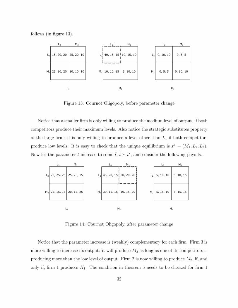
follows (in figure 13).

L3 M3 L3 M3 L3 M3

L2 15, 20, 20 25, 20, 10 L2 40, 15, 15 10, 15, 10 L2 0, 10, 10 0, 5, 5

M2 25, 10, 20 10, 10, 10 M2 10, 10, 15 5, 10, 10 M2 0, 5, 5 0, 10, 10

L1 M1 H1

Figure 13: Cournot Oligopoly, before parameter change

Notice that a smaller firm is only willing to produce the medium level of output, if both

competitors produce their maximum levels. Also notice the strategic substitutes property

of the large firm: it is only willing to produce a level other than L1 if both competitors

produce low levels. It is easy to check that the unique equilibrium is x∗ = (M1, L2, L3).

Now let the parameter t increase to some t, t ≻ t∗, and consider the following payoffs.

L3 M3 L3 M3 L3 M3

L2 20, 25, 25 25, 25, 15 L2 45, 20, 15 30, 20, 20 L2 5, 10, 10 5, 10, 15

M2 25, 15, 15 20, 15, 25 M2 30, 15, 15 10, 15, 20 M2 5, 15, 10 5, 15, 15

L1 M1 H1

Figure 14: Cournot Oligopoly, after parameter change

Notice that the parameter increase is (weakly) complementary for each firm. Firm 3 is

more willing to increase its output: it will produce M3 as long as one of its competitors is

producing more than the low level of output. Firm 2 is now willing to produce M2, if, and

only if, firm 1 produces H1. The condition in theorem 5 needs to be checked for firm 1

32

only (the firm with strategic substitutes). In this case, y1 = β1t(x∗

2, x∗3) = β1

t(L2, L3) = M1,

y2 = β2t(y1, x3) = β2

t(M1,M3) = L2, and y3 = β3

t(y1, x2) = β3

t(M1,M2) = M3. Therefore,

x∗1 = M1 � M1 = β1

t(L2,M3) = β1

t(y−1). Consequently, there is a higher equilibrium:

x = (M1, L2,M3).

The result in theorem 5 can be extended with similar intuition to best response cor-

respondences, as follows.

Theorem 6. Consider a parameterized GSH in which players 1, . . . , J have strategic

substitutes, and players J + 1, . . . , I have strategic complements and the strict single-

crossing property in (xi; t).

For every t∗ ≺ t and every x∗ ∈ E(t∗), let y = (yi)i∈I be defined as follows: yi = βi

t(x∗−i),

for i = 1, . . . , J , and yi = βi

t((yj)Jj=1; (xj)

Ij=J+1,j 6=i), for i = J + 1, . . . , I.

If for i = 1, . . . , J , x∗i � βi

t(y−i), then there is x ∈ E(t) such that x∗ � x.

Proof. Notice that for every i, x∗i � yi, as follows. For i = 1, . . . , J , using single-crossing

property, x∗i � β

i

t∗(x∗−i) � β

i

t(x∗−i) = yi. And for i = J + 1, . . . , I, x∗

i � βi

t∗(x∗−i) �

βi

t∗((yj)Jj=1; (xj)

Ij=J+1,j 6=i) � β

i

t((yj)Jj=1; (xj)

Ij=J+1,j 6=i) = yi, where the second inequality

follows from strategic complements, and the last inequality from single-crossing property.

For i = 1, . . . , I, let Bi = [x∗i , yi], and let B = ×I

i=1Bi. For i = 1, . . . , I, consider βit

on B−i. Then x∗i � βi

t(y−i) by assumption, and β

i

t(x∗−i) = yi, by definition. Therefore,

βit(B−i) ⊆ Bi; that is, β

itrestricted to B−i maps into Bi. Similarly, for i = J + 1, . . . , I,

consider βiton B−i. Strict single-crossing property in (xi; t) yields x∗

i � βi

t∗(x∗−i) �

βi

t(x∗

−i). Moreover, βit(y−i) = βi

t((yJj=1); (yj)

Ij=J+1,j 6=i) ⊑in βi

t((yJj=1); (xj)

Ij=J+1,j 6=i), where

the induced set order inequality follows from strategic complements. Therefore, βi

t(y−i) �

βi

t((yJj=1); (xj)

Ij=J+1,j 6=i) = yi. Thus, β

it(B−i) ⊆ Bi. Consequently, the joint best response

correspondence satisfies βt(B) ⊆ B; that is, the restriction of β to B is a self-map, and

applying Kakutani-Fan-Glicksberg’s theorem, there is a fixed point x ∈ E(t) such that

x∗ � x.

33

4 Conclusion

This paper studies games with strategic heterogeneity (GSH). Such games include cases in

which some players exhibit strategic complements and others exhibit strategic substitutes.

The equilibrium set in a GSH is totally unordered under mild assumptions. More-

over, parameterized GSH do not allow decreasing equilibrium selections, under mild as-

sumptions related to strategic substitutes for one player only. In general, this cannot

be strengthened to exhibit an increasing equilibrium selection. Finally, monotone com-

parative statics results are presented for games in which some players exhibit strategic

complements and others exhibit strategic substitutes. For two player games with linearly

ordered strategy spaces, there is a characterization of monotone comparative statics. More

generally, there are sufficient conditions. In both two-player and multi-player settings, the

conditions apply only to players exhibiting strategic substitutes. No additional conditions

are needed for players with strategic complements. Several examples highlight the results.

Our results show that it takes only a single player with strict strategic subsitutes to

destroy many of the nice properties of GSC, highlighting limits of techniques developed to

analyze GSC and the role of strategic substitutes in analyzing more heterogeneous cases.

Moreover, our results advance the study of GSH in several ways: showing uniqueness

of symmetric equilibria in some cases, making equilibrium search algorithms more effi-

cient, ruling out decreasing equilibrium selections, and providing conditions for monotone

comparative statics in games with both strategic complements and strategic substitutes.

34

References

Acemoglu, D., and M. K. Jensen (2009): “Aggregate comparative statics,” WorkingPaper, Department of Economics, University of Birmingham and MIT.

(2010): “Robust comparative statics in large static games,” Working Paper,Department of Economics, University of Birmingham.

Aliprantis, C. D., and K. C. Border (1994): Infinite Dimensional Analysis: AHitchhiker’s Guide. Springer-Verlag.

Amir, R. (1996): “Cournot Oligopoly and the Theory of Supermodular Games,” Gamesand Economic Behavior, 15, 132–148.

Amir, R., F. Garcia, and M. Knauff (2010): “Symmetry-breaking in two-playergames via strategic substitutes and diagonal nonconcavity: a synthesis,” Journal ofEconomic Theory, 145(5), 1968–1986.

Amir, R., and V. E. Lambson (2000): “On the Effects of Entry in Cournot Markets,”The Review of Economic Studies, 67(2), 235–254.

Baliga, S., and T. Sjostrom (2012): “The Strategy of Manipulating Conflict,” Amer-ican Economic Review, 102, 2897–2922.

Becker, G. S. (1968): “Crime and Punishment: An Economic Approach,” Journal ofPolitical Economy, 76, 169–217.

Bulow, J. I., J. D. Geanakoplos, and P. D. Klemperer (1985): “MultimarketOligopoly: Strategic Substitutes and Complements,” Journal of Political Economy,93(3), 488–511.

Dixit, A. (1987): “Strategic behavior in contests,” American Economic Review, 77(5),891–898.

Echenique, F. (2002): “Comparative statics by adaptive dynamics and the correspon-dence principle,” Econometrica, 70(2), 257–289.

(2004): “A characterization of strategic complementarities,” Games and Eco-nomic Behavior, 46(2), 325–347.

Edlin, A., and C. Shannon (1998): “Strict Monotonicity in Comparative Statics,”Journal of Economic Theory, 81(1), 201–219.

Fudenberg, D., and J. Tirole (1984): “The fat-cat effect, the puppy-dog ploy, andthe lean and hungry look,” American Economic Review, 74(2), 361–366.

35

Jensen, M. K. (2010): “Aggregative Games and Best-Reply Potentials,” EconomicTheory, 43(1), 45–66.

Lippman, S. A., J. W. Mamer, and K. F. McCardle (1987): “Comparative Staticsin non-cooperative games via transfinitely iterated play,” Journal of Economic Theory,41(2), 288–303.

Milgrom, P., and J. Roberts (1990): “Rationalizability, learning, and equilibrium ingames with strategic complementarities,” Econometrica, 58(6), 1255–1277.

(1994): “Comparing Equilibria,” American Economic Review, 84(3), 441–459.

Milgrom, P., and C. Shannon (1994): “Monotone Comparative Statics,” Economet-rica, 62(1), 157–180.

Quah, J. K.-H. (2007): “The Comparative Statics of Constrained Optimization Prob-lems,” Econometrica, 75(2), 401–431.

Quah, J. K.-H., and B. Strulovici (2009): “Comparative statics, informativeness,and the interval dominance order,” Econometrica, 77(6), 1949–1992.

Roy, S., and T. Sabarwal (2008): “On the (Non-)Lattice Structure of the EquilibriumSet in Games With Strategic Substitutes,” Economic Theory, 37(1), 161–169.

(2010): “Monotone comparative statics for games with strategic substitutes,”Journal of Mathematical Economics, 46(5), 793–806.

(2012): “Characterizing stability properties in games with strategic substitutes,”Games and Economic Behavior, 75(1), 337–353.

Schipper, B. C. (2003): “Submodularity and the evolution of Walrasian behavior,”International Journal of Game Theory, 32, 471–477.

Shadmehr, M., and D. Bernhardt (2011): “Collective Action with Uncertain Payoffs:Coordination, Public Signals, and Punishment Dilemmas,” American Political ScienceReview, 105, 829–851.

Shannon, C. (1995): “Weak and Strong Monotone Comparative Statics,” EconomicTheory, 5(2), 209–227.

Singh, N., and X. Vives (1984): “Price and quantity competition in a differentiatedduopoly,” Rand Journal of Economics, 13(4), 546–554.

Sobel, J. (1988): “Isotone comparative statics in supermodular games,” Mimeo. SUNYat Stony Brook.

Tombak, M. M. (2006): “Strategic Asymmetry,” Journal of Economic Behavior andOrganization, 61(3), 339–350.

36

Topkis, D. (1978): “Minimizing a submodular function on a lattice,” Operations Re-search, 26, 305–321.

(1979): “Equilibrium points in nonzero-sum n-person submodular games,” SIAMJournal on Control and Optimization, 17(6), 773–787.

(1998): Supermodularity and Complementarity. Princeton University Press.

Villas-Boas, J. M. (1997): “Comparative Statics of Fixed Points,” Journal of Eco-nomic Theory, 73(1), 183–198.

Vives, X. (1990): “Nash Equilibrium with Strategic Complementarities,” Journal ofMathematical Economics, 19(3), 305–321.

(1999): Oligopoly Pricing. MIT Press.

(2005): “Complementarities and Games: New Developments,” Journal of Eco-nomic Literature, 43(2), 437–479.

Zhou, L. (1994): “The Set of Nash Equilibria of a Supermodular Game is a CompleteLattice,” Games and Economic Behavior, 7(2), 295–300.

Zimper, A. (2007): “A fixed point characterization of the dominance-solvability of latticegames with strategic substitutes,” International Journal of Game Theory, 36(1), 107–117.

37

Appendix A

Roy and Sabarwal (2008) assume that the best response correspondence satisfies a never-increasing property, defined as follows. Let X be a lattice and T be a partially orderedset. A correspondence φ : T ։ X is never increasing, if for every t′ ≺ t′′, for everyx′ ∈ φ(t′), and for every x′′ ∈ φ(t′′), x′ 6� x′′.21 This property is satisfied in a GSS,but it excludes cases of interest when there are both strategic complements and strategicsubstitutes, as follows.

Recall that player i has quasi-strict strategic complements, if her best response,βi(x−i), is increasing in the completely lower than set order. Moreover, when best re-sponses are singleton-valued, player i has quasi-strict strategic complements, if, and onlyif, player i has strategic complements.

Proposition 1. Let Γ be a GSH in which all-but-one players exhibit quasi-strict strate-gic complements, and the remaining player has at least two actions. The best responsecorrespondence in such a game does not satisfy the never-increasing property.

Proof. Suppose, without loss of generality, that all-but-player-1 have quasi-strict strate-gic complements. Consider x′

1 ≺ x′′1 in X1, and x′

−1 ∈ X−1. Then (x′1, x

′−1) ≺ (x′′

1, x′−1).

Let y′1 ∈ β1(x′−1). For each i 6= 1, let x′

−i = (x′1, x

′−(1,i)) and x′′

−i = (x′′1, x

′−(1,i)). Then

for each i 6= 1, x′−i ≺ x′′

−i. For each such i, fix y′i ∈ βi(x′−i) and y′′i ∈ βi(x′′

−i) arbi-trarily. By quasi-strict strategic complements, y′i � y′′i . Thus, (x′

1, x′−1) ≺ (x′′

1, x′−1),

(y′1, y′−1) ∈ β(x′

1, x′−1), (y

′1, y

′′−1) ∈ β(x′′

1, x′−1), and (y′1, y

′−1) � (y′1, y

′′−1), contradicting the

never-increasing property.

Consequently, the case where all-but-one players exhibit quasi-strict strategic com-plements, and the remaining player has strategic substitutes is not covered by Roy andSabarwal (2008).

It is easy to see that the global nature of the definition of a never-increasing cor-respondence rules out additional cases of interest. The Cournot duopoly with spillovers(Example 3) provides an example. In this case, player 2 does not have quasi-strict strategiccomplements. Nevertheless, the best response correspondence does not satisfy the never-increasing property, because for example, for all ǫ > 0 sufficiently small, (1

2, 7) ≺ (1

2+ǫ, 7),

but β2(12) ≺ β2(1

2+ ǫ), and therefore, β(1

2, 7) ≺ β(1

2+ ǫ, 7). This occurs, because player 2

has quasi-strict strategic complements in a neighborhood of 12, even though he does not

have quasi-strict strategic complements globally. This is sufficient to violate the never-increasing property. This observation can be generalized. In particular, a similar proofshows that the conclusion of proposition 1 holds even when all-but-one players exhibit“local” quasi-strict strategic complements.

21When best responses are functions, this coincides with the definition of a not-increasing function,t′ ≺ t′′ ⇒ φ(t′) 6� φ(t′′), and in linearly ordered X , this is equivalent to a strictly decreasing function.

38

Appendix B

This appendix documents the lemmas needed to prove theorem 4 in the paper.

Lemma 1. Consider a two-player, parameterized GSH, in which player 1 has strict strate-gic substitutes, and player 2 has quasi-strict strategic complements. Suppose strategyspaces are linearly ordered. For every t∗ � t, for every x∗ ∈ E(t∗), and for every x ∈ E(t),x∗2 � x2.

Proof. Suppose x∗2 6� x2. Then linear order implies x2 ≺ x∗

2. Thus β1t∗(x

∗2) ⊑in β1

t(x∗

2) ⊏s

β1t(x2), where the induced set order inequality follows from single-crossing property in

(x1; t), and the strict set order inequality follows from strict strategic substitutes. This

implies x∗1 � β

1

t∗(x∗2) � β

1

t (x∗2) ≺ β1

t(x2) � x1. Therefore, β2

t∗(x∗1) ⊑in β2

t(x∗

1) ⊑c β2t(x1),

where the induced set order inequality follows from single-crossing property in (x2; t), andthe completely lower set order inequality follows from quasi-strict strategic complements.

This implies x∗2 � β

2

t∗(x∗1) � β

2

t (x∗1) � β2

t(x1) � x2, a contradiction.

Lemma 2. Consider a two-player, parameterized GSH, in which player 1 has strategicsubstitutes, and player 2 has strategic complements. Suppose strategy spaces are linearlyordered. For every t∗ � t, for every x∗ ∈ E(t∗), and for every x ∈ E(t),

x∗1 � x1 =⇒ x∗

1 � β1

tβ2

t(x∗

1).

Proof. x∗1 � x1 implies β2

t(x∗

1) � β2

t(x1) � x2, where the first inequality follows from

strategic complements. This, in turn, implies, x∗1 � x1 � β

1

t (x2) � β1

tβ2

t(x∗

1), where thelast inequality follows from strategic substitutes.

Lemma 3. Consider a two-player, parameterized GSH, in which player 1 has quasi-strictstrategic substitutes, and player 2 has strict strategic complements. Suppose strategy spacesare linearly ordered. For every t∗ � t, for every x∗ ∈ E(t∗), and for every x ∈ E(t),

x1 ≺ x∗1 =⇒ β

1

tβ2

t(x∗

1) ≺ x∗1.

Proof. Using strict strategic complements, x1 ≺ x∗1 implies β2

t(x1) ⊏s β2

t(x∗

1), and

therefore, x2 � β2

t (x1) ≺ β2

t(x∗

1). Using quasi-strict strategic substitutes, it follows that

β1t(β2

t(x∗

1)) ⊑c β1t(x2). Consequently, β

1

tβ2

t(x∗

1) � β1

t(x2) � x1 ≺ x∗

1.

These lemmas yield theorem 4 immediately.

39