“Hunger Games: Food Security and Strategic Preemptive

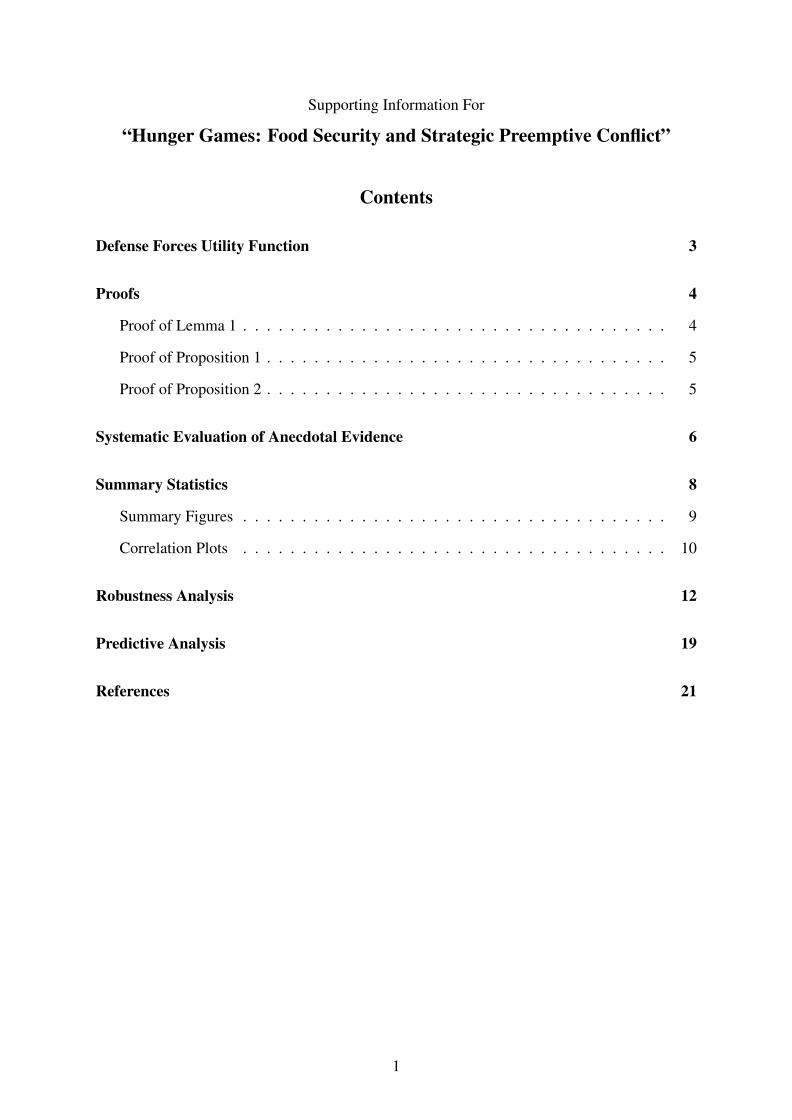
Supporting Information For

“Hunger Games: Food Security and Strategic Preemptive Conflict”

Contents

Defense Forces Utility Function 3

Proofs 4

Proof of Lemma 1 . . . . . . . . . . . . . . . . . . . . . . . . . . . . . . . . . . . . 4

Proof of Proposition 1 . . . . . . . . . . . . . . . . . . . . . . . . . . . . . . . . . . 5

Proof of Proposition 2 . . . . . . . . . . . . . . . . . . . . . . . . . . . . . . . . . . 5

Systematic Evaluation of Anecdotal Evidence 6

Summary Statistics 8

Summary Figures . . . . . . . . . . . . . . . . . . . . . . . . . . . . . . . . . . . . 9

Correlation Plots . . . . . . . . . . . . . . . . . . . . . . . . . . . . . . . . . . . . 10

Robustness Analysis 12

Predictive Analysis 19

References 21

1

This Appendix proceeds in five parts. In the first part, the utility of the defense forces, and

the derivations of the formal model’s equilibrium results and comparative statics are discussed

in detail. In the second part, a list of cases where it could be established that localities with

some levels of food production were targeted preemptively to reduce the other side’s levels

of food support is reported (Table A.1). The third part includes summary statistics of all the

variables used in the main analysis, prediction, and robustness models (Tables A.2 and A.3) as

well as figures showing the geospatial distribution of the dependent and explanatory variables;

and the frequency of conflict by grid cell and grid cell-year. Fourth, a set of sensitivity analyses

designed to show the robustness of the model presented in the primary analysis to a variety

of alternative specifications and the inclusion of different potential confounders are reported in

Tables A.4–A.9. Finally, the receiver-operator characteristics (ROC) curves of the model when

predicting raider attacks and defender responses for the years 2009-2010 are reported, as well

as a comparison between the area under the curve of the LQRM model and regular logit models

for both in and out-of-sample data.

2

Defense Forces Utility Function

Although the defense forces are not a strategic actor in this model and their behavior is assumed

to reflect the civilians’ actions, it is still worthwhile to briefly explain their utility function to

understand the model’s setting. To this end, let ν be the cost the defense forces d incur from

violent conflict M, for example, due to the loss of lives or equipment, such that ν > 0. In

addition, if they defeat the raiders with probability ρ , the defense forces get to keep their rents

R, e.g., through taxation, controlling natural resources production, etc., such that ρ×R. If they

lose, then they forfeit access to these rents, such that (1−ρ)×0. The defense forces’ d utility

function is thus:

Ud(M) = ρR−ν (1)

3

Proofs

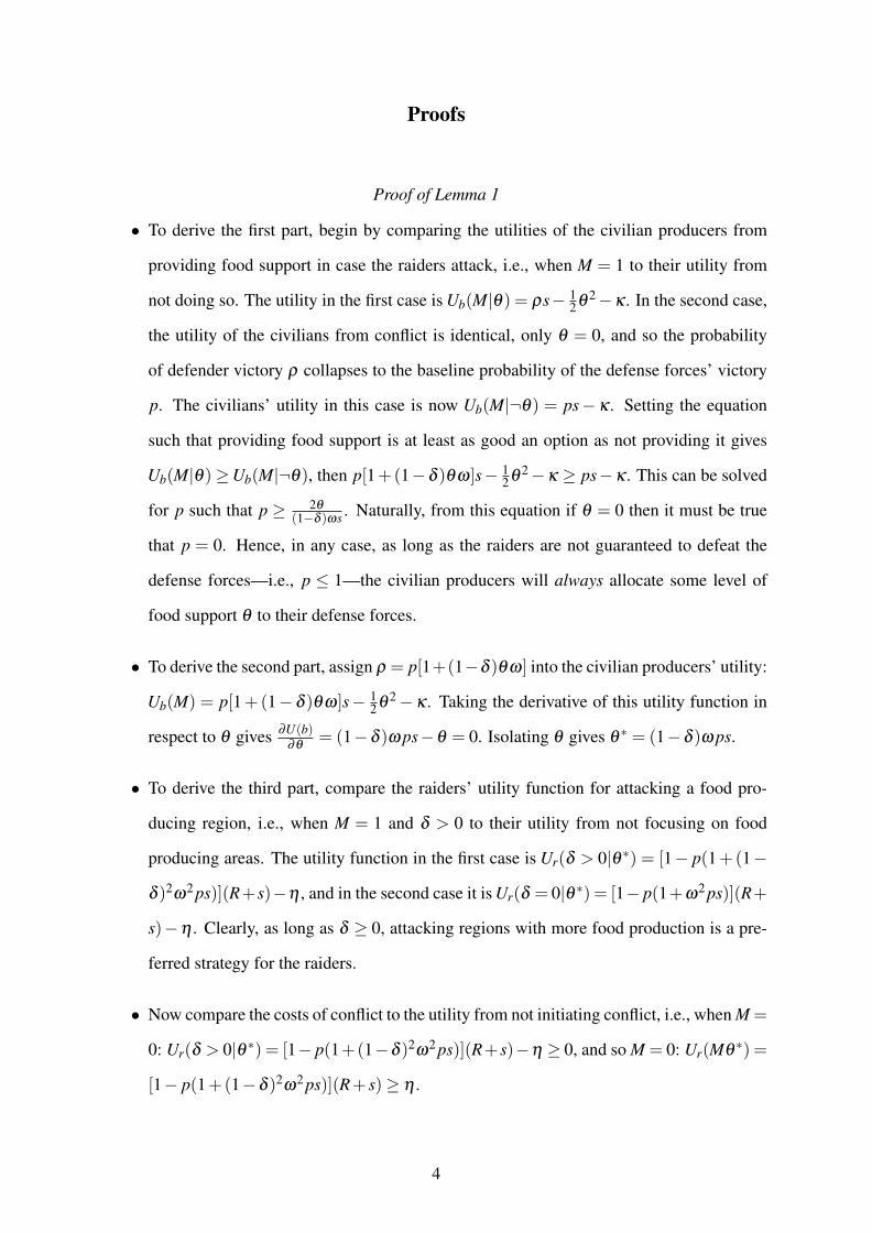
Proof of Lemma 1

• To derive the first part, begin by comparing the utilities of the civilian producers from

providing food support in case the raiders attack, i.e., when M = 1 to their utility from

not doing so. The utility in the first case is Ub(M|θ) = ρs− 12θ 2−κ . In the second case,

the utility of the civilians from conflict is identical, only θ = 0, and so the probability

of defender victory ρ collapses to the baseline probability of the defense forces’ victory

p. The civilians’ utility in this case is now Ub(M|¬θ) = ps− κ . Setting the equation

such that providing food support is at least as good an option as not providing it gives

Ub(M|θ)≥Ub(M|¬θ), then p[1+(1−δ )θω]s− 12θ 2−κ ≥ ps−κ . This can be solved

for p such that p ≥ 2θ

(1−δ )ωs . Naturally, from this equation if θ = 0 then it must be true

that p = 0. Hence, in any case, as long as the raiders are not guaranteed to defeat the

defense forces—i.e., p ≤ 1—the civilian producers will always allocate some level of

food support θ to their defense forces.

• To derive the second part, assign ρ = p[1+(1−δ )θω] into the civilian producers’ utility:

Ub(M) = p[1+(1− δ )θω]s− 12θ 2−κ . Taking the derivative of this utility function in

respect to θ gives ∂U(b)∂θ

= (1−δ )ω ps−θ = 0. Isolating θ gives θ ∗ = (1−δ )ω ps.

• To derive the third part, compare the raiders’ utility function for attacking a food pro-

ducing region, i.e., when M = 1 and δ > 0 to their utility from not focusing on food

producing areas. The utility function in the first case is Ur(δ > 0|θ ∗) = [1− p(1+(1−

δ )2ω2 ps)](R+s)−η , and in the second case it is Ur(δ = 0|θ ∗) = [1− p(1+ω2 ps)](R+

s)−η . Clearly, as long as δ ≥ 0, attacking regions with more food production is a pre-

ferred strategy for the raiders.

• Now compare the costs of conflict to the utility from not initiating conflict, i.e., when M =

0: Ur(δ > 0|θ ∗) = [1− p(1+(1−δ )2ω2 ps)](R+ s)−η ≥ 0, and so M = 0: Ur(Mθ ∗) =

[1− p(1+(1−δ )2ω2 ps)](R+ s)≥ η .

4

Proof of Proposition 1

To obtain these results take the partial derivative of θ ∗ in respect to p, ω , and s when M = 1.

• In respect to p: ∂θ∗

∂ p = s(1− δ )ω ≥ 0 because δ < 1; and so θ ∗ increases with higher

probabilities of the defense forces d’s victory.

• In respect to ω: ∂θ∗

∂ω= s(1− δ )p ≥ 0 because δ < 1; and so θ ∗ increases when food

support is more important for improving the defense forces’ overall probability of victory.

• In respect to s, ∂θ∗

∂ s = (1− δ )ω p ≥ 0 because δ < 1; and so θ ∗ increases with higher

value of land s.

Proof of Proposition 2

• To obtain these results, first take the partial derivative of the raiders’ utility when M = 1

in respect to δ and compare it to 0 (the utility of the raiders when M = 0). Clearly,∂U(r)

∂δ= 2ω2 p2s(s+R)(1−δ )> 0 because δ < 1; and so the raiders’ utility from initiat-

ing conflict increases the stronger the effect of violence is on reducing food support.

• To obtain the second part of this proposition and show that the raiders will be more likely

to initiate conflict if it has a stronger effect on diminishing the defense forces’ probability

of victory, take the derivative of the raiders’ utility from conflict in respect to p to isolate

p∗, and then take the derivative of p∗ in respect δ . Taking the derivative of Ur(M|θ ∗) in

respect to p and isolating p gives p∗ =− 12(d−1)2sω2 , which shows that—unsurprisingly—

the utility of the raiders from conflict decreases with higher probability of the defense

forces’ victory. The derivative in respect to p∗ should thus show how the utility from

raiding in respect to the probability of the defense forces’ victory changes with higher

levels of δ : ∂ p∗∂δ

= sω2(1−δ )≥ 0 because δ ≤ 1, and so the raiders will initiate conflict

even with higher probability of the defense forces’ victory if conflict has a strong effect

on reducing the food support available to the defense forces.

5

Systematic Evaluation of Anecdotal Evidence

Table A.1 provides a list of cases where preemptive conflict over food resources has occurred.

Distinguishing possessive conflict—i.e. conflict designed to increase one’s own food security

levels—from preemptive conflict—i.e., conflict designed to decrease one’s rivals’ food security

levels—is complicated, because most conflict events over food resources is likely to involve

elements of both. I thus only included in Table A.1 cases where it was explicitly stated that

the aim of using violence was to weaken or hurt the other side by appropriating or destroying

locally produced food resources.

6

Table A.1: A Partial List of Preemptive Conflicts over Food Security

Country Target Raiders Resource Source

Angola civilian farmers, gov. troops UNITA rebels crops Macrae and Zwi (1992)

East Timor local civilians rebel militias livestock The New Zealand Herald (2002)

El Salvador local civilians gov. troops crops Messer and Cohen (2006)

Ethiopia (Tigre and Eritrea) civilians, EPLF and TPLF troops the Derg crops, livestock Keller (1992)

Ghana Fulani herders Farmers crops, livestock Tonah (2006)

India (Bastar) farmers, civil defense forces Naxalite rebels crops Sundar (2007)Planning Commission of India (2008)

Italy (Sicily) Mafia families Mafia families livestock Blok (1969)

Kenya Pokot/Turkana militias Pokot/Turkana militias livestock Clemens (2013)

Mozambique local civilians, gov. troops RENAMO crops Hultman (2009)

Nigeria (Biafra) Biafra civilians Nigerian military crops, stockpiles Jacobs (1987)

Nigeria Fulani herders Farmers crops, livestock Ofuoku (2009)

Peru (Tacuna and Arequipa) farmers, civil defense forces Túpac Amaru rebels crops, livestock Masterson (1991); Walker (1999)

Sierra Leone SLA/CDF RUF crops Mkandawire (2002); Keen (2005)

Somalia (Somaliland) local civilians pro-Barre militias crops, livestock Ahmed and Green (1999)

Sudan (Darfur) local civilians, JEM, SLA Sudanese gov./ethnic militias crops, livestock de Waal (2005)

Sudan ethnic Dinka militias/Sudanese gov. livestock Barrow (1996)

Sudan/S. Sudan S. Sudan Sudanese pastoralists livestock Leff (2009)

Thailand (Songkhla) farmers, civil defense forces BRN-C rebels crops The Nation (2004)Montesano and Jory (2008)

Uganda local civilians, LRA Ugandan military crops, stockpiles Doom and Vlassenroot (1999)

Vietnam local civilians, Viet Cong U.S. military crops Leebaw (2014)

7

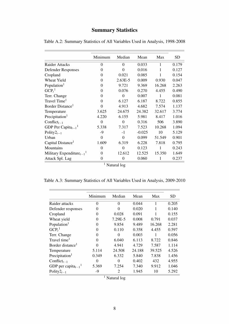
Summary Statistics

Table A.2: Summary Statistics of All Variables Used in Analysis, 1998-2008

Minimum Median Mean Max SD

Raider Attacks 0 0 0.033 1 0.179Defender Responses 0 0 0.016 1 0.127Cropland 0 0.021 0.085 1 0.154Wheat Yield 0 2.63E-5 0.009 0.930 0.047Population1 0 9.721 9.369 16.268 2.263GCPt

1 0 0.076 0.270 4.455 0.490Terr. Change 0 0 0.007 1 0.081Travel Time1 0 6.127 6.187 8.722 0.855Border Distance1 0 4.913 4.682 7.574 1.137Temperature 3.625 24.675 24.382 32.617 3.774Precipitation1 4.220 6.155 5.981 8.417 1.016Conflictt−1 0 0 0.316 506 3.890GDP Per Capitat−1

1 5.338 7.317 7.523 10.268 1.094Polity2t−1 -9 -1 -0.025 10 5.129Urban 0 0 0.099 51.549 0.901Capital Distance1 1.609 6.319 6.228 7.818 0.795Mountains 0 0 0.123 1 0.243Military Expendituret−1

1 0 12.612 12.525 15.350 1.649Attack Spl. Lag 0 0 0.060 1 0.237

1 Natural log

Table A.3: Summary Statistics of All Variables Used in Analysis, 2009-2010

Minimum Median Mean Max SD

Raider attacks 0 0 0.044 1 0.205Defender responses 0 0 0.020 1 0.140Cropland 0 0.028 0.091 1 0.155Wheat yield 0 7.29E-5 0.008 0.791 0.037Population1 0 9.854 9.489 16.268 2.281GCPt

1 0 0.110 0.358 4.455 0.597Terr. Change 0 0 0.003 1 0.056Travel time1 0 6.040 6.113 8.722 0.846Border distance1 0 4.941 4.729 7.587 1.114Temperature 5.114 24.508 24.188 39.525 4.526Precipitation1 0.349 6.332 5.840 7.838 1.456Conflictt−1 0 0 0.402 432 4.955GDP per capitat−1

1 5.369 7.254 7.340 9.912 1.046Polity2t−1 -9 2 1.945 10 5.292

1 Natural log

8

Summary Figures

Figure A.1: The Regional Distribution of Staple Cropland and Wheat Yields, 1998-2008

Cropland, 1998-2008 Wheat Yields, 1998-2008

Figure A.2: The Regional Distribution of Attacks by Raiders and Responses by Defense Forces,1998-2008

Raider Attacks, 1998-2008 Defender Responses, 1998-2008

9

Figure A.3: The Regional Distribution of Attacks by Raiders and Responses by Defense Forces,2009-2010

Raider Attacks, 2009-2010 Defender Responses, 2009-2010

Figure A.4: The Distribution of Raider Attacks and Defense Forces Response by Grid Cell andCell-Year, 1998-2008

Distribution by Grid Cell Distribution by Cell-Year

Correlation Plots

To provide illustrative evidence regarding the effect of the local food indicators discussed above

on the different categories of the dependent variable, the correlations between (i) cropland lev-

10

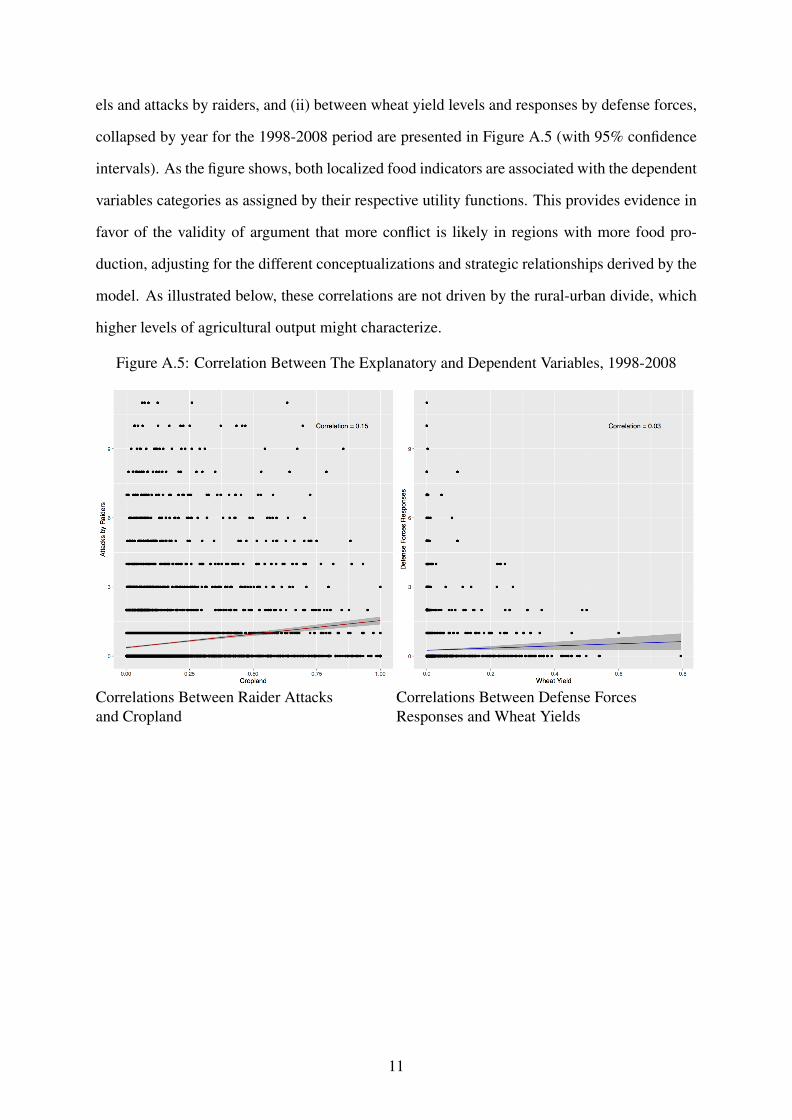
els and attacks by raiders, and (ii) between wheat yield levels and responses by defense forces,

collapsed by year for the 1998-2008 period are presented in Figure A.5 (with 95% confidence

intervals). As the figure shows, both localized food indicators are associated with the dependent

variables categories as assigned by their respective utility functions. This provides evidence in

favor of the validity of argument that more conflict is likely in regions with more food pro-

duction, adjusting for the different conceptualizations and strategic relationships derived by the

model. As illustrated below, these correlations are not driven by the rural-urban divide, which

higher levels of agricultural output might characterize.

Figure A.5: Correlation Between The Explanatory and Dependent Variables, 1998-2008

Correlations Between Raider Attacksand Cropland

Correlations Between Defense ForcesResponses and Wheat Yields

11

Robustness Analysis

This robustness section includes six alternative replications of the primary analysis to test its

sensitivity to alternative mechanisms and specification choices. First, the effect of urbanization

on the utilities of the raiders and the civilians is more throughly taken into account by including

an indicator measuring the level of urbanization in each grid cell in the equations capture the

raiders’ and defense forces’ utilities in Table A.4. Second, numerous studies have equated a

higher likelihood of conflict with lower state capacity levels (e.g., Fearon and Laitin, 2003).

To account for this possibility, Table A.5 estimates the primary model with the inclusion of

distance to capital and the percentage of a given cell that is mountainous, in a manner used

in past studies (Fearon and Laitin, 2003; Fjelde and Hultman, 2014). Third, attacks in certain

grid cells might be caused because attacks nearby push raiders to attack these cells due to

their vicinity, i.e., conflict can simply spill over from a neighboring cell. To account for this

possibility, Table A.6 includes spatial lags of raider attacks in the raiders’ utility function.

Fourth, recall that non of the independent variables (excluding the lag of the dependent vari-

able) were lagged due to the potential misspecification issues and inferential biases that might

result (Bellemare, Masaki and Pepinsky, Forthcoming). Nevertheless, to show that my results

are robust to this decision, a model where all time varying indicators are lagged by one year is

reported in Table A.7. Fifth, the size of the state’s military might influence the raiders’ decision

whether to initiate conflict or pursue more peaceful solutions under the status quo. To account

for this possibility, a model that includes lagged military expenditure in the raiders’ utility from

the status quo (obtained from the Correlated of War dataset Singer, Bremer and Stucky, 1972)

is reported in Table A.8 to account for the potential effects of military (i.e., defense force) size

on the raiders’ decision to attack. Finally, to show that the results are not driven by my choice

of controls or the number of indicators included in the model, a baseline specification of the

primary analysis using only a small number of variables in the utility functions of the both

the raiders and the civilians. Crucially, the significance and sign of cropland and wheat yields

is consistent across these different specifications, which additionally confirms the argument

developed in the main paper.

12

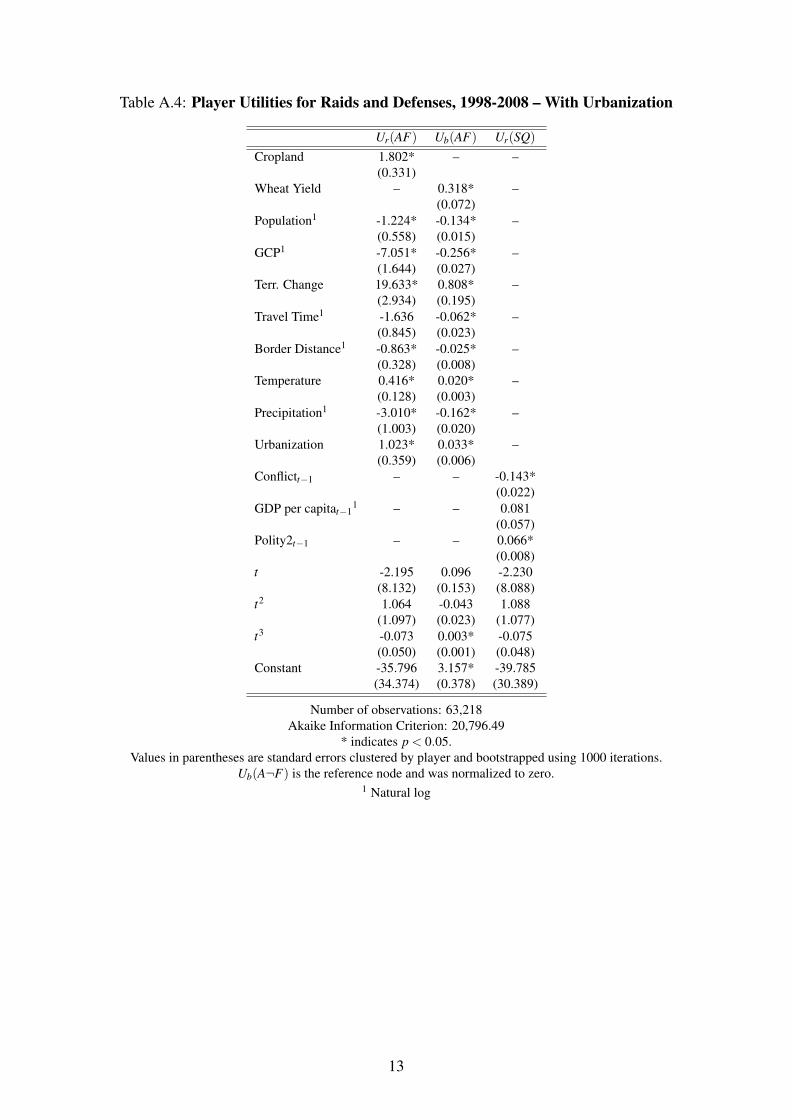
Table A.4: Player Utilities for Raids and Defenses, 1998-2008 – With Urbanization

Ur(AF) Ub(AF) Ur(SQ)

Cropland 1.802* – –(0.331)

Wheat Yield – 0.318* –(0.072)

Population1 -1.224* -0.134* –(0.558) (0.015)

GCP1 -7.051* -0.256* –(1.644) (0.027)

Terr. Change 19.633* 0.808* –(2.934) (0.195)

Travel Time1 -1.636 -0.062* –(0.845) (0.023)

Border Distance1 -0.863* -0.025* –(0.328) (0.008)

Temperature 0.416* 0.020* –(0.128) (0.003)

Precipitation1 -3.010* -0.162* –(1.003) (0.020)

Urbanization 1.023* 0.033* –(0.359) (0.006)

Conflictt−1 – – -0.143*(0.022)

GDP per capitat−11 – – 0.081

(0.057)Polity2t−1 – – 0.066*

(0.008)t -2.195 0.096 -2.230

(8.132) (0.153) (8.088)t2 1.064 -0.043 1.088

(1.097) (0.023) (1.077)t3 -0.073 0.003* -0.075

(0.050) (0.001) (0.048)Constant -35.796 3.157* -39.785

(34.374) (0.378) (30.389)

Number of observations: 63,218Akaike Information Criterion: 20,796.49

* indicates p < 0.05.Values in parentheses are standard errors clustered by player and bootstrapped using 1000 iterations.

Ub(A¬F) is the reference node and was normalized to zero.1 Natural log

13

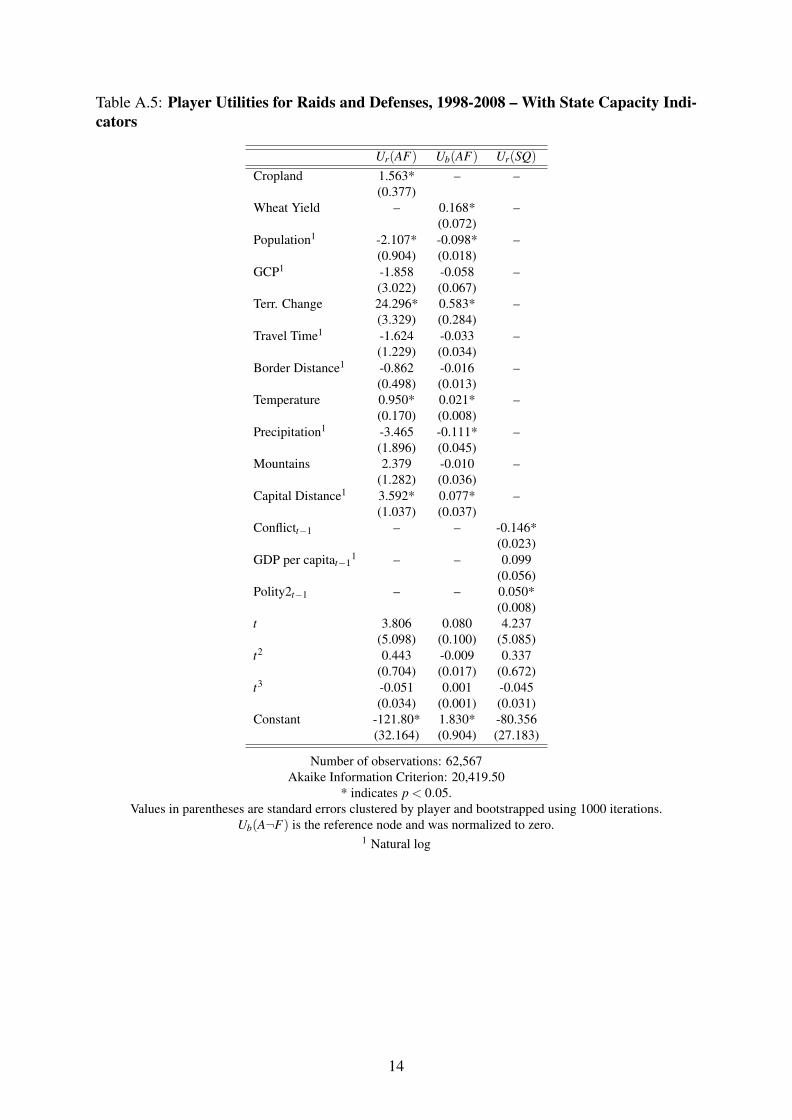
Table A.5: Player Utilities for Raids and Defenses, 1998-2008 – With State Capacity Indi-cators


Cropland 1.563* – –(0.377)

Wheat Yield – 0.168* –(0.072)

Population1 -2.107* -0.098* –(0.904) (0.018)

GCP1 -1.858 -0.058 –(3.022) (0.067)

Terr. Change 24.296* 0.583* –(3.329) (0.284)

Travel Time1 -1.624 -0.033 –(1.229) (0.034)

Border Distance1 -0.862 -0.016 –(0.498) (0.013)

Temperature 0.950* 0.021* –(0.170) (0.008)

Precipitation1 -3.465 -0.111* –(1.896) (0.045)

Mountains 2.379 -0.010 –(1.282) (0.036)

Capital Distance1 3.592* 0.077* –(1.037) (0.037)

Conflictt−1 – – -0.146*(0.023)

GDP per capitat−11 – – 0.099

(0.056)Polity2t−1 – – 0.050*

(0.008)t 3.806 0.080 4.237

(5.098) (0.100) (5.085)t2 0.443 -0.009 0.337

(0.704) (0.017) (0.672)t3 -0.051 0.001 -0.045

(0.034) (0.001) (0.031)Constant -121.80* 1.830* -80.356

(32.164) (0.904) (27.183)




14

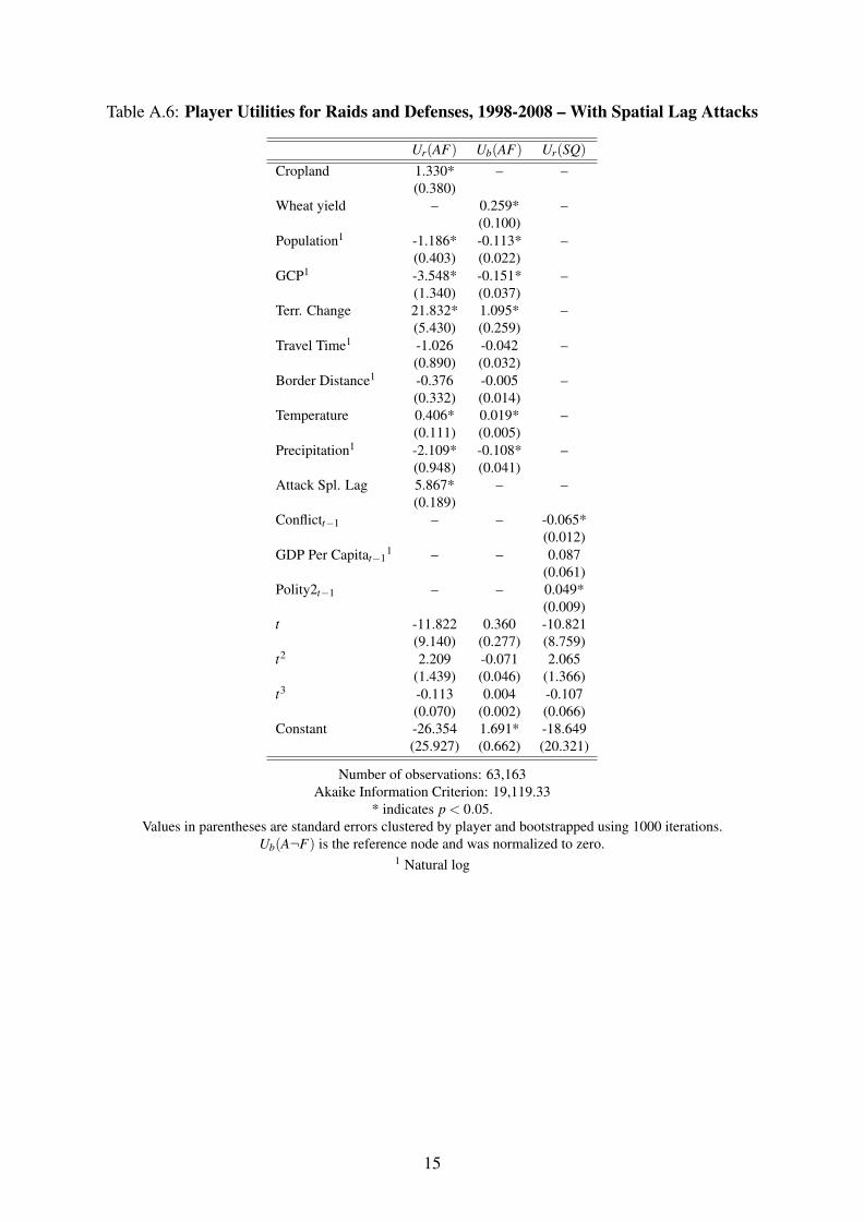
Table A.6: Player Utilities for Raids and Defenses, 1998-2008 – With Spatial Lag Attacks


Cropland 1.330* – –(0.380)

Wheat yield – 0.259* –(0.100)

Population1 -1.186* -0.113* –(0.403) (0.022)

GCP1 -3.548* -0.151* –(1.340) (0.037)

Terr. Change 21.832* 1.095* –(5.430) (0.259)

Travel Time1 -1.026 -0.042 –(0.890) (0.032)

Border Distance1 -0.376 -0.005 –(0.332) (0.014)

Temperature 0.406* 0.019* –(0.111) (0.005)

Precipitation1 -2.109* -0.108* –(0.948) (0.041)

Attack Spl. Lag 5.867* – –(0.189)

Conflictt−1 – – -0.065*(0.012)

GDP Per Capitat−11 – – 0.087

(0.061)Polity2t−1 – – 0.049*

(0.009)t -11.822 0.360 -10.821

(9.140) (0.277) (8.759)t2 2.209 -0.071 2.065

(1.439) (0.046) (1.366)t3 -0.113 0.004 -0.107

(0.070) (0.002) (0.066)Constant -26.354 1.691* -18.649

(25.927) (0.662) (20.321)




15

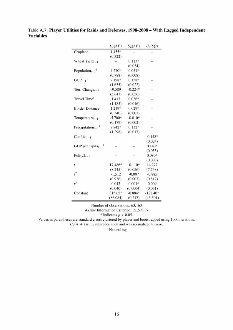
Table A.7: Player Utilities for Raids and Defenses, 1998-2008 – With Lagged IndependentVariables


Cropland 1.455* – –(0.322)

Wheat Yieldt−1 – 0.113* –(0.034)

Populationt−11 4.270* 0.051* –

(0.788) (0.008)GCPt−1

1 7.198* 0.158* –(1.655) (0.022)

Terr. Changet−1 -9.589 -0.224* –(5.647) (0.056)

Travel Time1 1.413 0.036* –(1.185) (0.016)

Border Distance1 1.219* 0.029* –(0.540) (0.007)

Temperaturet−1 -5.700* -0.010* –(0.179) (0.002)

Precipitationt−11 7.842* 0.132* –

(1.298) (0.017)Conflictt−1 – – -0.148*

(0.024)GDP per capitat−1

1 – – 0.140*(0.055)

Polity2t−1 – – 0.080*(0.008)

t 17.486* -0.110* 14.277(8.245) (0.056) (7.738)

t2 -1.512 -0.007 -0.885(0.936) (0.007) (0.817)

t3 0.043 0.001* 0.009(0.040) (0.0004) (0.031)

Constant 315.65* -0.884* -128.40*(86.084) (0.217) (45.501)




16

Table A.8: Player Utilities for Raids and Defenses, 1998-2008 – With Military Expenditure


Cropland 1.376* – –(0.324)

Wheat Yield – 0.189* –(0.074)

Population1 -2.257* -0.108* –(0.556) (0.017)

GCP1 -5.856* -0.139* –(1.376) (0.024)

Terr. Change 23.231* 0.568* –(3.224) (0.174)

Travel Time1 -2.066* -0.045* –(0.830) (0.023)

Border Distance1 -0.914* -0.012 –(0.297) (0.008)

Temperature 0.729* 0.020* –(0.131) (0.004)

Precipitation1 -3.871* -0.126* –(1.029) (0.022)

Conflictt−1 – – -0.145*(0.021)

GDP Per Capitat−11 – – 0.257*

(0.055)Polity2t−1 – – 0.056*

(0.008)Mil. Expt−1 – – -0.280*

(0.029)t 3.578 -0.092 4.578

(6.560) (0.125) (6.453)t2 0.568 -0.009 0.361

(0.938) (0.021) (0.901)t3 -0.062 0.001 -0.051

(0.045) (0.001) (0.042)Constant -82.572* 2.713* -78.229*

(29.310) (0.370) (26.043)




17

Table A.9: Player Utilities for Raids and Defenses, 1998-2008 – Baseline Model


Cropland 1.529* – –(0.309)

Wheat Yield – 0.283* –(0.071)

Population1 -2.151* -0.159* –(0.615) (0.020)

Temperature 0.614 0.025* –(0.161) (0.004)

Precipitation1 -1.831* -0.108* –(0.721) (0.018)

Conflictt−1 – – -0.208*(0.027)

GDP Per Capitat−11 – – 0.123*

(0.042)Polity2t−1 – – 0.075*

(0.008)t 6.767 0.008 -17.798

(7.552) (0.130) (15.115)t2 -0.318 -0.044* 3.527*

(0.921) (0.021) (2.101)t3 -0.005 0.003* -0.189**

(0.041) (0.001) (0.096)Constant -76.377 2.859* 61.260

(45.476) (0.337) (36.381)




18

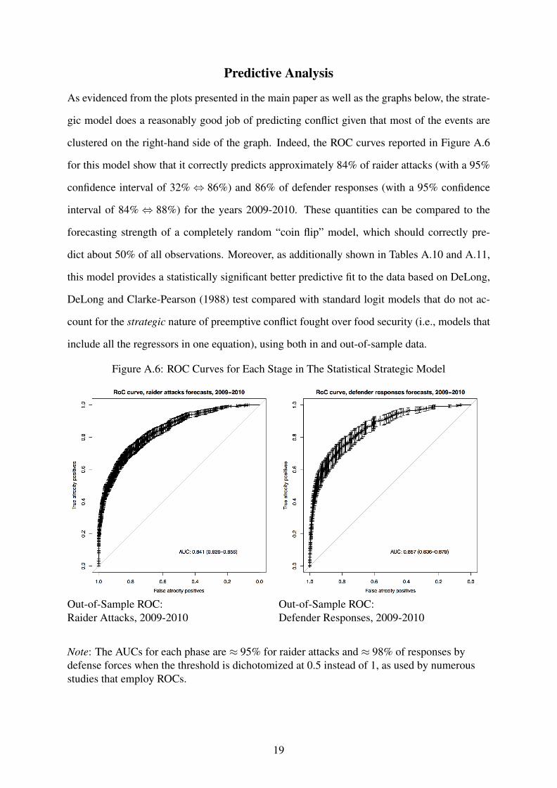
Predictive Analysis

As evidenced from the plots presented in the main paper as well as the graphs below, the strate-

gic model does a reasonably good job of predicting conflict given that most of the events are

clustered on the right-hand side of the graph. Indeed, the ROC curves reported in Figure A.6

for this model show that it correctly predicts approximately 84% of raider attacks (with a 95%

confidence interval of 32%⇔ 86%) and 86% of defender responses (with a 95% confidence

interval of 84%⇔ 88%) for the years 2009-2010. These quantities can be compared to the

forecasting strength of a completely random “coin flip” model, which should correctly pre-

dict about 50% of all observations. Moreover, as additionally shown in Tables A.10 and A.11,

this model provides a statistically significant better predictive fit to the data based on DeLong,

DeLong and Clarke-Pearson (1988) test compared with standard logit models that do not ac-

count for the strategic nature of preemptive conflict fought over food security (i.e., models that

include all the regressors in one equation), using both in and out-of-sample data.

Figure A.6: ROC Curves for Each Stage in The Statistical Strategic Model

Out-of-Sample ROC:Raider Attacks, 2009-2010

Out-of-Sample ROC:Defender Responses, 2009-2010

Note: The AUCs for each phase are ≈ 95% for raider attacks and ≈ 98% of responses bydefense forces when the threshold is dichotomized at 0.5 instead of 1, as used by numerousstudies that employ ROCs.

19

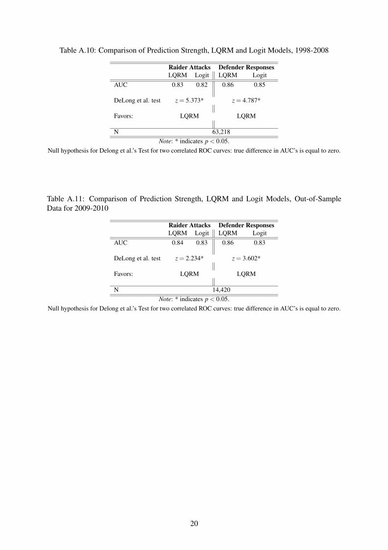
Table A.10: Comparison of Prediction Strength, LQRM and Logit Models, 1998-2008

Raider Attacks Defender ResponsesLQRM Logit LQRM Logit

AUC 0.83 0.82 0.86 0.85

DeLong et al. test z = 5.373* z = 4.787*

Favors: LQRM LQRM

N 63,218Note: * indicates p < 0.05.

Null hypothesis for Delong et al.’s Test for two correlated ROC curves: true difference in AUC’s is equal to zero.

Table A.11: Comparison of Prediction Strength, LQRM and Logit Models, Out-of-SampleData for 2009-2010

Raider Attacks Defender ResponsesLQRM Logit LQRM Logit

AUC 0.84 0.83 0.86 0.83

DeLong et al. test z = 2.234* z = 3.602*

Favors: LQRM LQRM

N 14,420Note: * indicates p < 0.05.

Null hypothesis for Delong et al.’s Test for two correlated ROC curves: true difference in AUC’s is equal to zero.

20

References

Ahmed, Ismail I and Reginald Herbold Green. 1999. “The heritage of war and state collapse

in Somalia and Somaliland: local-level effects, external interventions and reconstruction.”

Third World Quarterly 20(1):113–127.

Barrow, Greg. 1996. “ANCIENT CATTLE CULTURE UNDER THREAT FROM WAR.” The

Guardian, April 4, 1996.

Bellemare, Marc F., Takaaki Masaki and Thomas B. Pepinsky. Forthcoming. “Lagged Explana-

tory Variables and the Estimation of Causal Effects.” Journal of Politics .

Blok, Anton. 1969. “Peasants, Patrons, and Brokers in Western Sicily.” Anthropological

Quarterly 42(3):155–170.

Clemens. 2013. “GUNS, LAND, AND VOTES: CATTLE RUSTLING AND THE POLITICS

OF BOUNDARY (RE)MAKING IN NORTHERN KENYA.” African Affairs (112):216–

237.

de Waal, Alex. 2005. Famine that Kills: Darfur, Sudan. Oxford: Oxford University Press.

DeLong, Elisabeth R., David M. DeLong and Daniel L. Clarke-Pearson. 1988. “Comparing the

areas under two or more correlated receiver operating characteristic curves: a nonparametric

approach.” Biometrics 44:837–845.

Doom, Ruddy and Koen Vlassenroot. 1999. “Konny’s Message: A New Koine? The Lord’s

Resistance Army in Northern Uganda.” African Affairs 98:5–36.

Fearon, James D. and David D. Laitin. 2003. “Ethnicity, Insurgency, and Civil War.” American

Political Science Review 97(1):75–90.

Fjelde, Hanne and Lisa Hultman. 2014. “Weakening the Enemy: A Disaggregated Study of

Violence against Civilians in Africa.” Journal of Conflict Research 58(7):1230–1257.

Hultman, Lisa. 2009. “The Power to Hurt in Civil War: The Strategic Aim of RENAMO

Violence.” Journal of Southern African Studies 35(4):821–834.

21

Jacobs, Dan. 1987. The Brutality of Nations. New York: Alfred Knopf.

Keen, David. 2005. Conflict and Collusion in Sierra Leone. Suffolk: James Currey.

Keller, Edmond J. 1992. “Drought, War, and the Politics of Famine in Ethiopia and Eritrea.”

The Journal of Modern African Studies 30(4):609–624.

Leebaw, Bronwyn. 2014. “Scorched Earth: Environmental War Crimes and International Jus-

tice.” Perspectives on Politics 12(4):770–788.

Leff, Jonah. 2009. “Pastoralists at War: Violence and Security in the Kenya-Sudan-Uganda

Border Region.” International Journal of Conflict and Violence 3(2):188–203.

Macrae, Joanna and Anthony B. Zwi. 1992. “Food as an Instrument of War in Contemporary

African Famines: A Review of the Evidence.” Disasters 16(4):299–321.

Masterson, Daniel M. 1991. Militarism and Politics in Latin America: Peru from Sánchez

Cerro to Sendero Luminoso. New York: Greenwood Press.

Messer, Ellen and Marc. J. Cohen. 2006. “Conflict, Food Insecurity, and Globalization.” FCND

Discussion Paper 206, International Food Policy Research Institute.

Mkandawire, Thandika. 2002. “The terrible toll of post-colonial ?rebel movements? in Africa:

towards an explanation of the violence against the peasantry.” The Journal of Modern African

Studies 40(2):181–215.

Montesano, M. and Patrick Jory. 2008. Thai South and Malay North: Ethnic Interactions on a

Plural Peninsular. Singapore: NUS Press.

Ofuoku, A.U. 2009. “The Role of Community Development Committees in Farmer-Herder

Conflicts in Central Agricultural Zone of Delta State, Nigeria.” International Journal of Rural

Studies 16(1):1–10.

Planning Commission of India. 2008. “Development Challenges in Extremist Affected Areas:

Report of an Expert Group.” Official Report.

22

Singer, J. David, Stuart Bremer and John Stucky. 1972. Capability Distribution, Uncertainty,

and Major Power War, 1820-1965. In Peace, War, and Numbers, ed. Bruce Russett. Beverly

Hills: Sage.

Sundar, Nandini. 2007. Subalterns and Sovereigns: An Anthropological History of Bastar

(1854-2006), 2nd Edition. Delhi: Oxford University Press.

The Nation. 2004. “Food fights between BRN-C and Farmers in Songkhla.” The Nation 19

November 2004, pp.A-2.

The New Zealand Herald. 2002. “Timor peacekeepers farewelled as ‘epitome of modern

force’.” November 15, 2002.

Tonah, Steve. 2006. “Migration and Farmer-Herder Conflicts in Ghana’s Volta Basin.”

Canadian Journal of African Studies 40(1):152–178.

Walker, C.F. 1999. Smoldering Ashes: Cuzco and the Creation of Republican Peru. Durham:

Duke University Press.

23

Documents

“Hunger Games: Food Security and Strategic Preemptive