Embed Size (px)
Citation preview

GAME THEORY AND INDUSTRIAL
ORGANISATION
David Kelsey and Surajeet ChakravartyDepartment of Economics
University of Exeter
January 2012

0.1 INTRODUCTION
1. Dominance (DK)
2. Nash Equilibrium (SC)
3. Games with Incomplete Information (DK)
4. Repeated Games (DK)
5. Static Oligopoly (SC) Bertrand and Cournot models with product differ-entiation.
6. Investment and Barriers to Entry (SC)
7. Entry, Accommodation and Exit (SC)
8. Predatory Pricing (DK)
• *Eichberger, J. Game Theory for Economists, Academic Press., 1993.
• Osborne, M. J. and A. Rubinstein, A Course in Game Theory, MIT Press, 1994.
• Myerson, Game Theory, Havard UP. 1991.
• Luce and Raiffa Games and Decisions, Dover (1957 reprinted 1989).
website http://people.exeter.ac.uk/dk210/gt-12.html
Please prepare Problem Sheet 1, questions 1-3 for 2nd February.
1 DOMINANT STRATEGIES
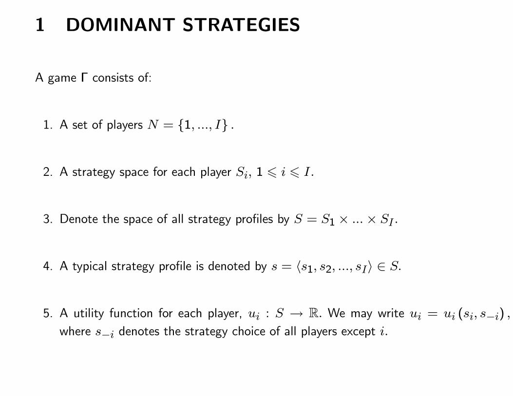
A game Γ consists of:
1. A set of players N = {1, ..., I} .
2. A strategy space for each player Si, 1 � i � I.
3. Denote the space of all strategy profiles by S = S1 × ...× SI.
4. A typical strategy profile is denoted by s = 〈s1, s2, ..., sI〉 ∈ S.
5. A utility function for each player, ui : S → R. We may write ui = ui (si, s−i) ,
where s−i denotes the strategy choice of all players except i.
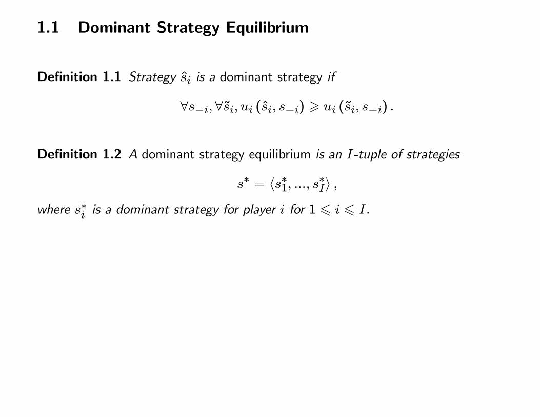
1.1 Dominant Strategy Equilibrium
Definition 1.1 Strategy si is a dominant strategy if
∀s−i,∀si, ui (si, s−i) � ui (si, s−i) .
Definition 1.2 A dominant strategy equilibrium is an I-tuple of strategies
s∗ = 〈s∗1, ..., s∗I〉 ,
where s∗i is a dominant strategy for player i for 1 � i � I.
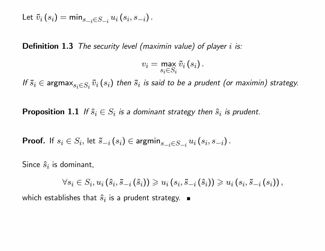
Let vi (si) = mins−i∈S−i ui (si, s−i) .
Definition 1.3 The security level (maximin value) of player i is:
vi = maxsi∈Si
vi (si) .
If si ∈ argmaxsi∈Si vi (si) then si is said to be a prudent (or maximin) strategy.
Proposition 1.1 If si ∈ Si is a dominant strategy then si is prudent.
Proof. If si ∈ Si, let s−i (si) ∈ argmins−i∈S−i ui (si, s−i) .
Since si is dominant,
∀si ∈ Si, ui (si, s−i (si)) � ui (si, s−i (si)) � ui (si, s−i (si)) ,
which establishes that si is a prudent strategy.
1.2 Examples of games with dominant strategy equilibria
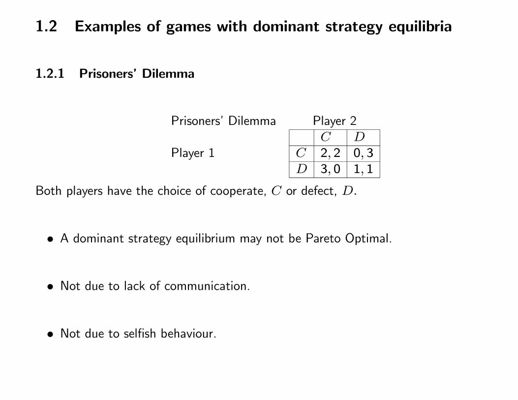
1.2.1 Prisoners’ Dilemma
Prisoners’ Dilemma Player 2
Player 1C D
C 2, 2 0, 3D 3, 0 1, 1
Both players have the choice of cooperate, C or defect, D.
• A dominant strategy equilibrium may not be Pareto Optimal.
• Not due to lack of communication.
• Not due to selfish behaviour.
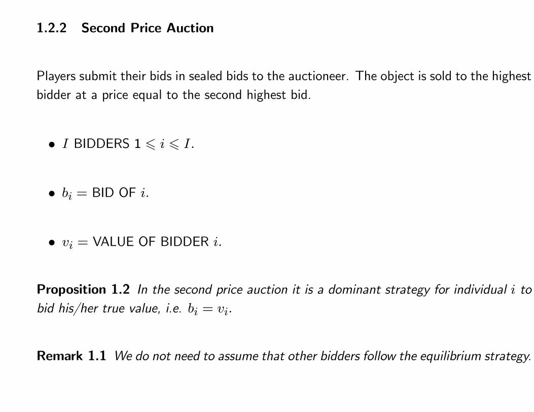
1.2.2 Second Price Auction
Players submit their bids in sealed bids to the auctioneer. The object is sold to the highest
bidder at a price equal to the second highest bid.
• I BIDDERS 1 � i � I.
• bi = BID OF i.
• vi = VALUE OF BIDDER i.
Proposition 1.2 In the second price auction it is a dominant strategy for individual i to
bid his/her true value, i.e. bi = vi.
Remark 1.1 We do not need to assume that other bidders follow the equilibrium strategy.
1.2.3 Clarke-Groves Mechanism for Public Goods
The government has to decide whether of not to provide a discrete public good at cost
K.
There are I citizens.
Individual i has (true) value vi of the public good.
Individual i sends a report ri of his/her value to the government.
The government wants to provide the good if∑Ii=1 vi � K.
If the good is provided individual i pays a tax ti = K −∑j �=i rj.
Proposition 1.3 Reporting ri = vi is a dominant strategy for individual i.
Proof. . Consider individual i. There are three cases to consider:
Case 1 Suppose∑j �=i rj < K < vi +
∑j �=i rj
If i reports ri = vi then the project will go ahead and (s)he will pay a tax ti = K −∑j �=i rj < vi, thus receiving positive net benefit.
The same holds for any ri such that ri +∑j �=i rj > K.
Suppose now (s)he reports ri < vi such that ri +∑j �=i rj < K.
Then the public good will not be provided, there will be no taxes giving i a net pay-off of
0.
Thus in this case reporting ri = vi is a best response regardless of the opponents’ strategy.
Case 2 Suppose vi +∑j �=i rj < K.
If i reports ri = vi then the public good will not be provided, giving i a net pay-off of 0.
The same holds for any ri such that ri +∑j �=i rj < K.
Now assume i reports ri > vi such that ri +∑j �=i rj > K.
Then the public good will be provided. However i will face a tax bill ofK−∑j �=i rj > vi.
Thus reporting ri yields a negative pay-off.
Again reporting ri = vi is a best response regardless of the opponent’s strategy.
Case 3 Suppose K <∑j �=i rj < vi +
∑j �=i rj.
In this case the public good will be provided and j will get a subsidy ti =∑j �=i rj −K
regardless of what (s)he reports. Thus ri = vi is a best response in this case.
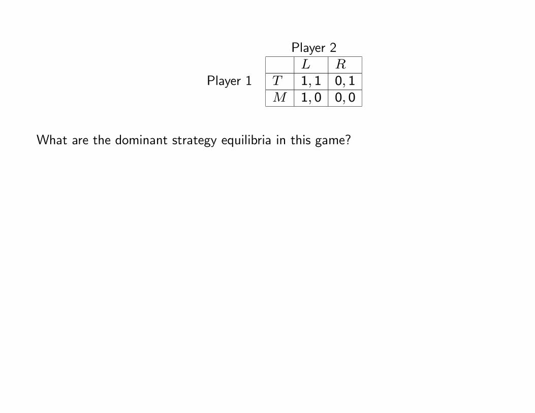
Player 2
Player 1L R
T 1, 1 0, 1M 1, 0 0, 0
What are the dominant strategy equilibria in this game?
1.2.4 UNIQUENESS
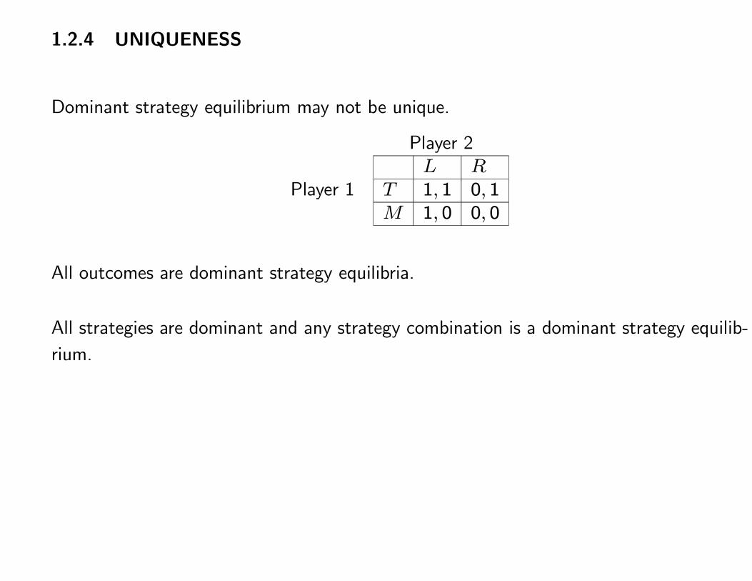
Dominant strategy equilibrium may not be unique.
Player 2
Player 1L R
T 1, 1 0, 1M 1, 0 0, 0
All outcomes are dominant strategy equilibria.
All strategies are dominant and any strategy combination is a dominant strategy equilib-
rium.
1.3 CONCLUSION
The disadvantage of dominant strategy equilibrium is that existence is not guaranteed.
Dominant Strategy equilibrium has the advantage that:
• It is a strong equilibrium concept.
— You do not need to know your opponents play the equilibrium strategy or even
are rational.
— Do not need to know your opponents pay-offs.
• Some important economic examples
• If you are designing a game e.g. incentives for employees, then you may choose that
game to have a dominant strategy equilibrium.
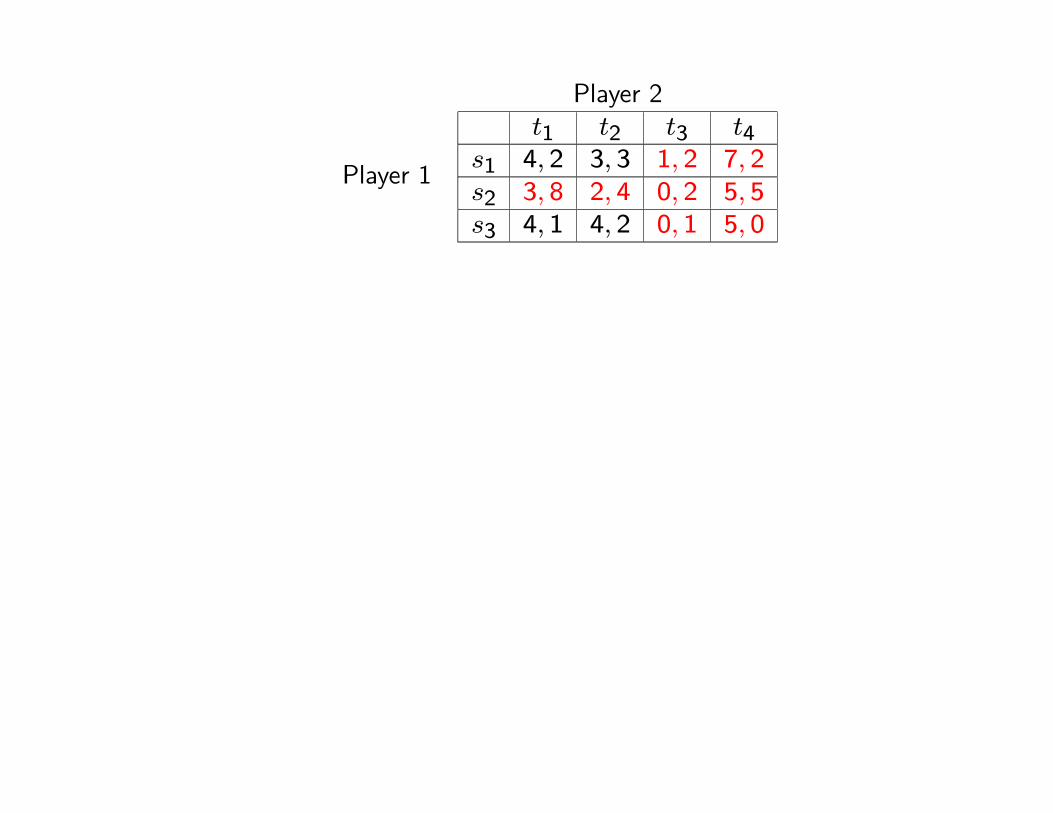
1.4 ITERATED DOMINANCE
Eichberger, section 3.2
Kreps, Ch. 12.
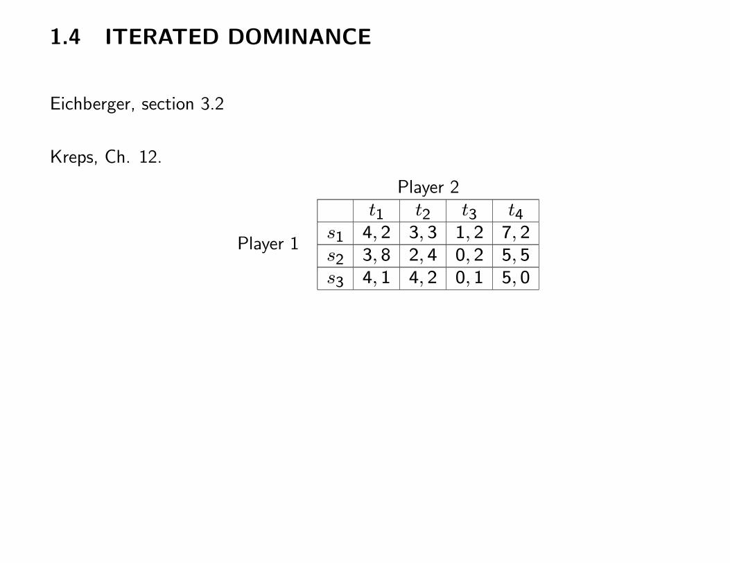
Player 2
Player 1
t1 t2 t3 t4s1 4, 2 3, 3 1, 2 7, 2s2 3, 8 2, 4 0, 2 5, 5s3 4, 1 4, 2 0, 1 5, 0
Player 2
Player 1
t1 t2 t3 t4s1 4, 2 3, 3 1, 2 7, 2s2 3, 8 2, 4 0, 2 5, 5s3 4, 1 4, 2 0, 1 5, 0
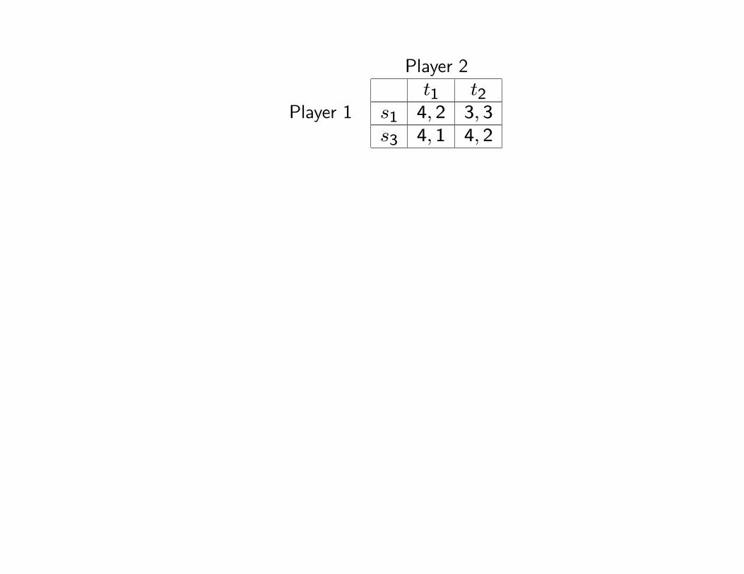
Player 2
Player 1t1 t2
s1 4, 2 3, 3s3 4, 1 4, 2
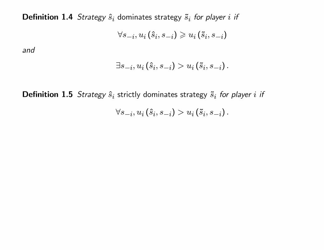
Definition 1.4 Strategy si dominates strategy si for player i if
∀s−i, ui (si, s−i) � ui (si, s−i)
and
∃s−i, ui (si, s−i) > ui (si, s−i) .
Definition 1.5 Strategy si strictly dominates strategy si for player i if
∀s−i, ui (si, s−i) > ui (si, s−i) .
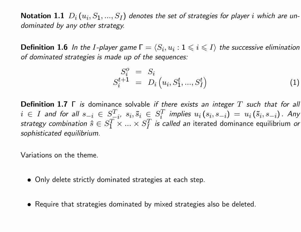
Notation 1.1 Di (ui, S1, ..., SI) denotes the set of strategies for player i which are un-
dominated by any other strategy.
Definition 1.6 In the I-player game Γ = 〈Si, ui : 1 � i � I〉 the successive elimination
of dominated strategies is made up of the sequences:
Soi = SiSt+1i = Di
(ui, S
t1, ..., S
tI
)(1)
Definition 1.7 Γ is dominance solvable if there exists an integer T such that for all
i ∈ I and for all s−i ∈ ST−i, si, si ∈ STi implies ui (si, s−i) = ui (si, s−i) . Any
strategy combination s ∈ ST1 × ... × STI is called an iterated dominance equilibrium or
sophisticated equilibrium.
Variations on the theme.
• Only delete strictly dominated strategies at each step.
• Require that strategies dominated by mixed strategies also be deleted.
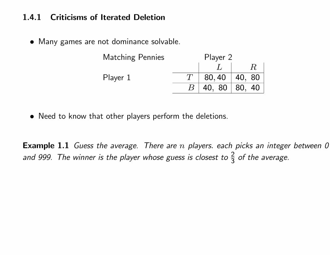
1.4.1 Criticisms of Iterated Deletion
• Many games are not dominance solvable.
Matching Pennies Player 2
Player 1L R
T 80, 40 40, 80B 40, 80 80, 40
• Need to know that other players perform the deletions.
Example 1.1 Guess the average. There are n players. each picks an integer between 0
and 999. The winner is the player whose guess is closest to 23 of the average.
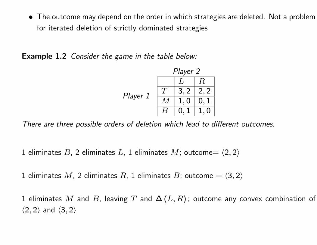
• The outcome may depend on the order in which strategies are deleted. Not a problem
for iterated deletion of strictly dominated strategies
Example 1.2 Consider the game in the table below:
Player 2
Player 1
L RT 3, 2 2, 2M 1, 0 0, 1B 0, 1 1, 0
There are three possible orders of deletion which lead to different outcomes.
1 eliminates B, 2 eliminates L, 1 eliminates M ; outcome= 〈2, 2〉
1 eliminates M , 2 eliminates R, 1 eliminates B; outcome = 〈3, 2〉
1 eliminates M and B, leaving T and ∆(L,R) ; outcome any convex combination of
〈2, 2〉 and 〈3, 2〉
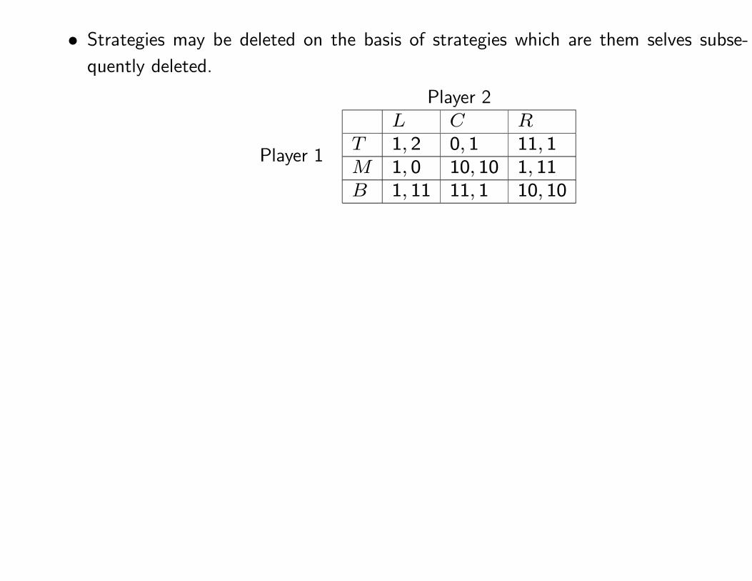
• Strategies may be deleted on the basis of strategies which are them selves subse-
quently deleted.
Player 2
Player 1
L C RT 1, 2 0, 1 11, 1M 1, 0 10, 10 1, 11B 1, 11 11, 1 10, 10
1.4.2 Existence
One problem with using iterated dominance as a solution concept is that there are relatively
few general existence results. The following are the only reasonably general results which
can be obtained.
A game has strategic complements if there is an ordering on the strategy space and
when one player increases his/her strategy this gives an incentive for his/her rivals to also
increase their strategies.
For example Bertrand Oligopoly.
Theorem 1.1 Let Γ be a game of strategic complements then then set of strategies
remaining after iterated deletion of dominated strategies lie between the highest and
lowest Nash equilibrium.
If Nash equilibrium is unique then it is also an iterated dominance equilibrium.

Definition 1.8 An extensive form game Γ satisfies the one to one assumption if for any
two terminal nodes m,m′ and any player i ui (m) = ui(m′)
implies uj (m) = uj(m′)
for 1 � j � I.
Theorem 1.2 Let Γ be an extensive form game of complete and perfect information
which satisfies the one to one assumption. Then the normal form of Γ is dominance
solvable.
Outline of proof
• Look at nodes whose successors are terminal nodes. Whoever has the move at these
nodes picks whichever terminal node gives them the highest utility.
• Now consider all nodes whose successors are either terminal nodes or next to terminal
nodes. There is now a best choice for whoever has to choose at these nodes.
• Continue in this way until all choices have been made.
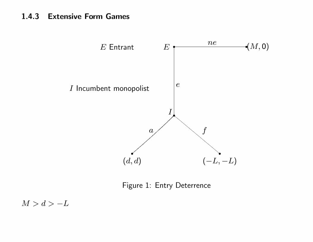
1.4.3 Extensive Form Games
��
�
�
�������������
(M, 0)
(d, d) (−L,−L)
ne
e
a f
I
EE Entrant
I Incumbent monopolist
Figure 1: Entry Deterrence
M > d > −L
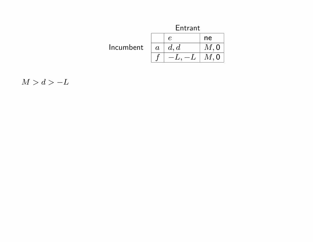
Entrant
Incumbente ne
a d, d M, 0f −L,−L M, 0
M > d > −L
�
��
�
�
�
�
� � �
� �
��
�
�
�
�
�� �
�
��
�
�
��
1,1 0,3 2,2 98,98 97,100 99,99 98,101
100,1001 2 1 2121
� � �
D D D D D D D
A A A AAA
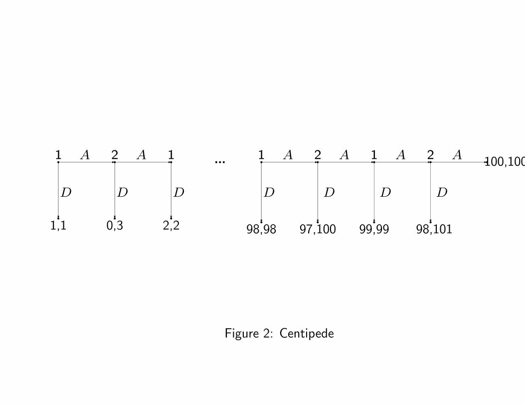
Figure 2: Centipede
1.4.4 COURNOT DUOPOLY
See Fudenberg and Tirole p. 47.
With Linear demand and constant marginal costs, Cournot duopoly is dominance solvable.
Suppose there are 2 firms who can produce at zero marginal cost.
The demand curve is given by p = 1− q1 − q2.
Firms choose outputs from the interval [0,K] , K � 1.
Firms aim to maximise profit.

Proposition 1.4 Under the above assumptions, Cournot duopoly is dominance solvable.
Proof. Firm 1’s profit is given by: π1 = q1 (1− q1 − q2) .
The first order condition for profit maximisation is:
(1− q1 − q2)− q1 = 1− 2q1 − q2 = 0.
Hence 1’s reaction curve is given by r1 (q2) =1−q22 .
Similarly 2’s reaction curve is given by r2 (q1) =1−q12 .

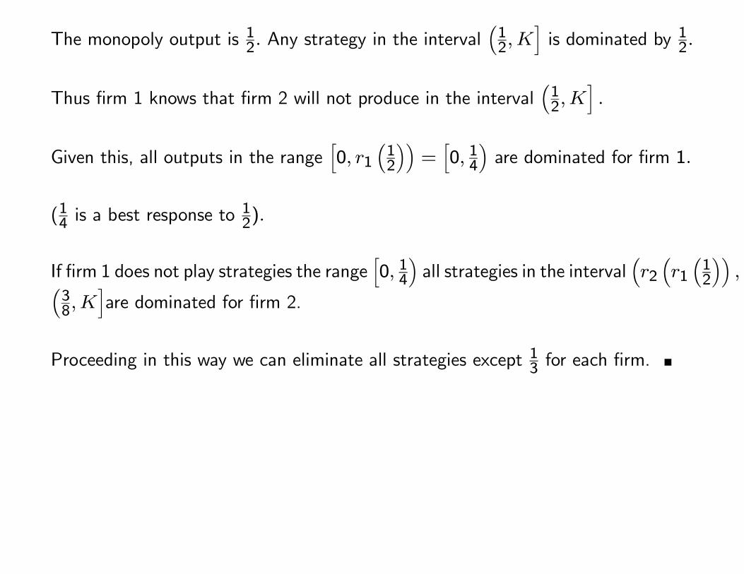
The monopoly output is 12. Any strategy in the interval(12,K
]is dominated by 12.
Thus firm 1 knows that firm 2 will not produce in the interval(12,K
].
Given this, all outputs in the range[0, r1
(12
))=[0, 14
)are dominated for firm 1.
(14 is a best response to 12).
If firm 1 does not play strategies the range[0, 14
)all strategies in the interval
(r2(r1(12
)),K
(38,K
]are dominated for firm 2.
Proceeding in this way we can eliminate all strategies except 13 for each firm.
Extensions
• Whenever demand is linear and marginal cost is constant Cournot duopoly is domi-
nance solvable.
• If there are multiple equilibria, Cournot oligopoly is not dominance solvable.
• If there are 3 (or more) firms, Cournot oligopoly is not dominance solvable.
1.5 CONCLUSION
Iterated dominance provides a solution concept which uses a relatively weak notion of
rationality.
• No general existence results.
• The solution is less attractive when it relies on many rounds of deletion e.g. in the
centipede game.
• Chess is dominance solvable.
— However this tells us very little about chess.
2 NASH EQUILIBRIUM
References
• *Eichberger Ch. 4.
• Osborne and Rubinstein, Chs. 2-3.
• Goeree and Holt, (2001), ‘Ten Little Treasures of Game Theory’, American Economic
Review.
• For a detailed account of how to find a Nash equilibrium see Myerson pp. 88-129.
Recall ui (si, s−i) = utility (or payoff) function of player i.
s−i = profile of strategies chosen by players other than i.
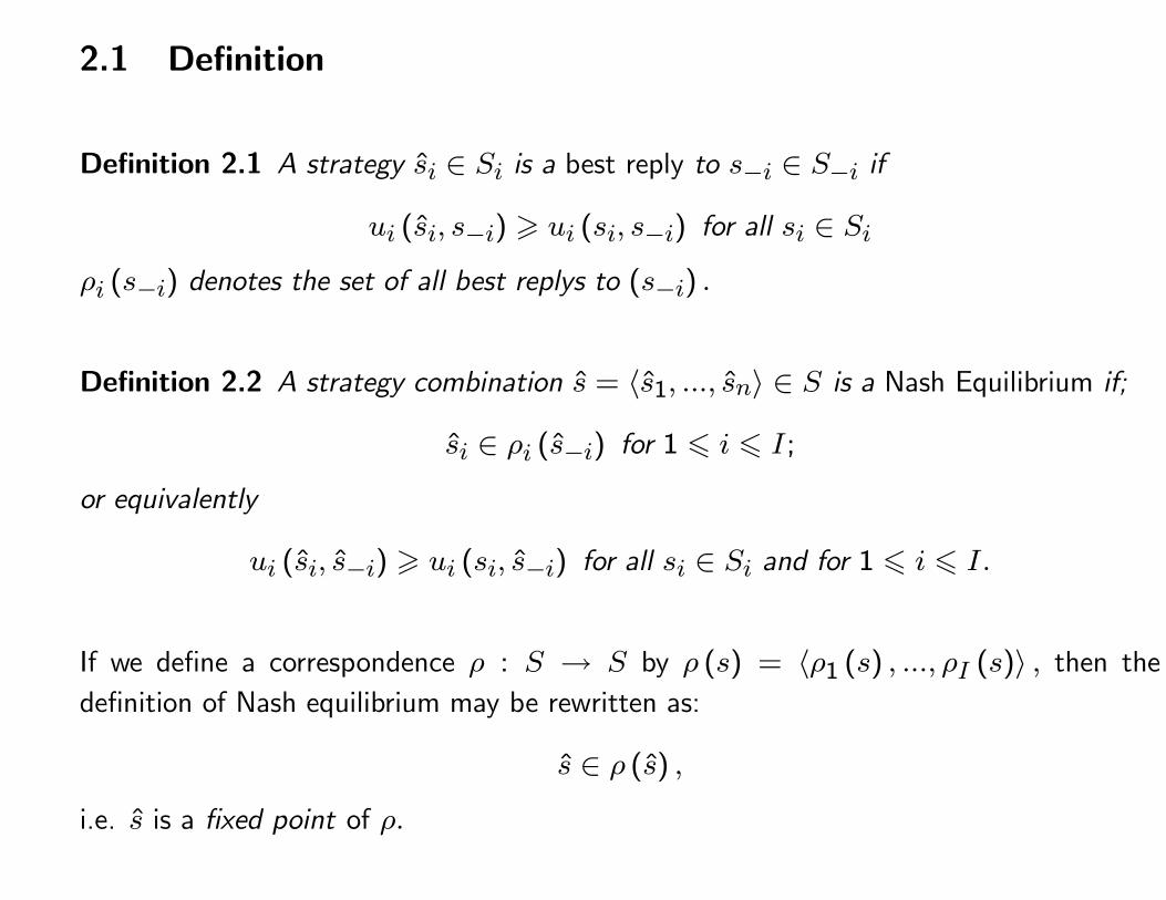
2.1 Definition
Definition 2.1 A strategy si ∈ Si is a best reply to s−i ∈ S−i if
ui (si, s−i) � ui (si, s−i) for all si ∈ Si
ρi (s−i) denotes the set of all best replys to (s−i) .
Definition 2.2 A strategy combination s = 〈s1, ..., sn〉 ∈ S is a Nash Equilibrium if;
si ∈ ρi (s−i) for 1 � i � I;
or equivalently
ui (si, s−i) � ui (si, s−i) for all si ∈ Si and for 1 � i � I.
If we define a correspondence ρ : S → S by ρ (s) = 〈ρ1 (s) , ..., ρI (s)〉 , then the
definition of Nash equilibrium may be rewritten as:
s ∈ ρ (s) ,
i.e. s is a fixed point of ρ.
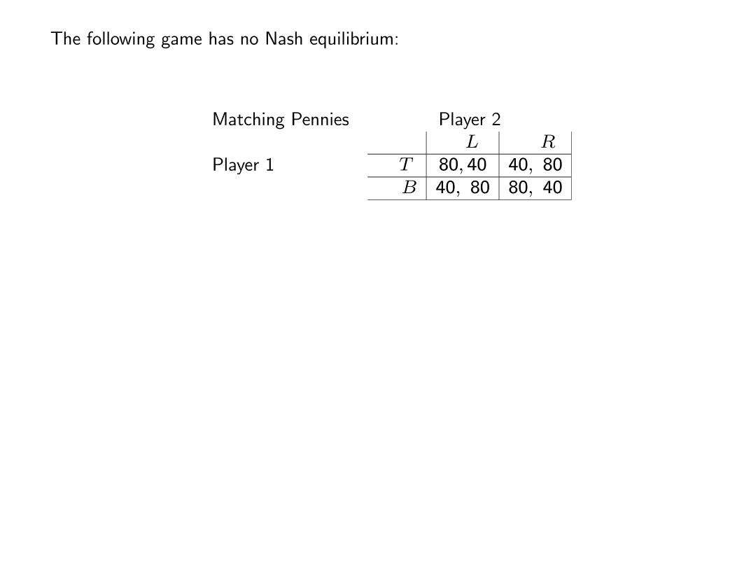
The following game has no Nash equilibrium:
Matching Pennies Player 2
Player 1L R
T 80, 40 40, 80B 40, 80 80, 40
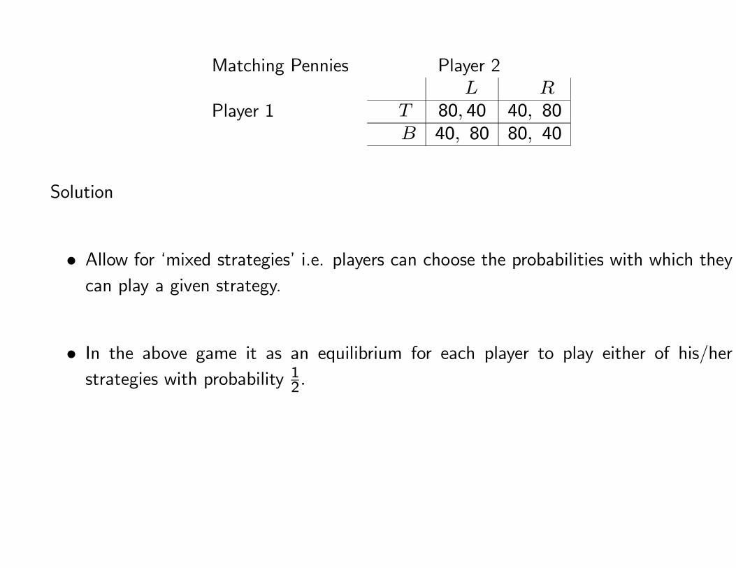
Matching Pennies Player 2
Player 1L R
T 80, 40 40, 80B 40, 80 80, 40
Solution
• Allow for ‘mixed strategies’ i.e. players can choose the probabilities with which they
can play a given strategy.
• In the above game it as an equilibrium for each player to play either of his/her
strategies with probability 12.
2.2 Existence of Nash Equilibrium
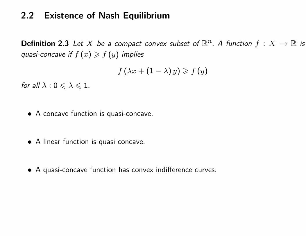
Definition 2.3 Let X be a compact convex subset of Rn. A function f : X → R is
quasi-concave if f (x) � f (y) implies
f (λx+ (1− λ) y) � f (y)
for all λ : 0 � λ � 1.
• A concave function is quasi-concave.
• A linear function is quasi concave.
• A quasi-concave function has convex indifference curves.
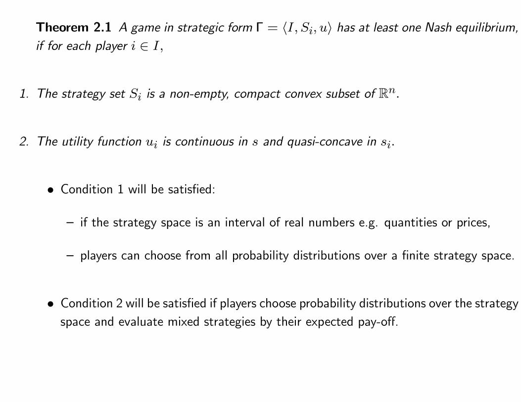
Theorem 2.1 A game in strategic form Γ = 〈I, Si, u〉 has at least one Nash equilibrium,
if for each player i ∈ I,
1. The strategy set Si is a non-empty, compact convex subset of Rn.
2. The utility function ui is continuous in s and quasi-concave in si.
• Condition 1 will be satisfied:
— if the strategy space is an interval of real numbers e.g. quantities or prices,
— players can choose from all probability distributions over a finite strategy space.
• Condition 2 will be satisfied if players choose probability distributions over the strategy
space and evaluate mixed strategies by their expected pay-off.
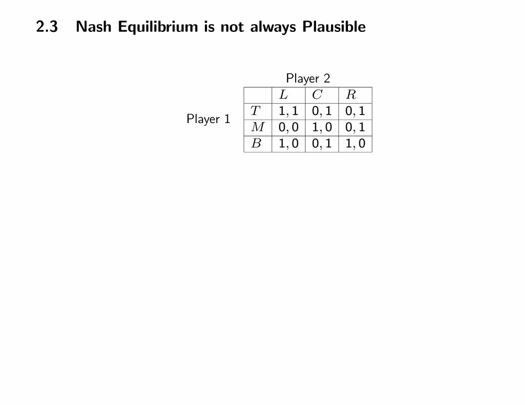
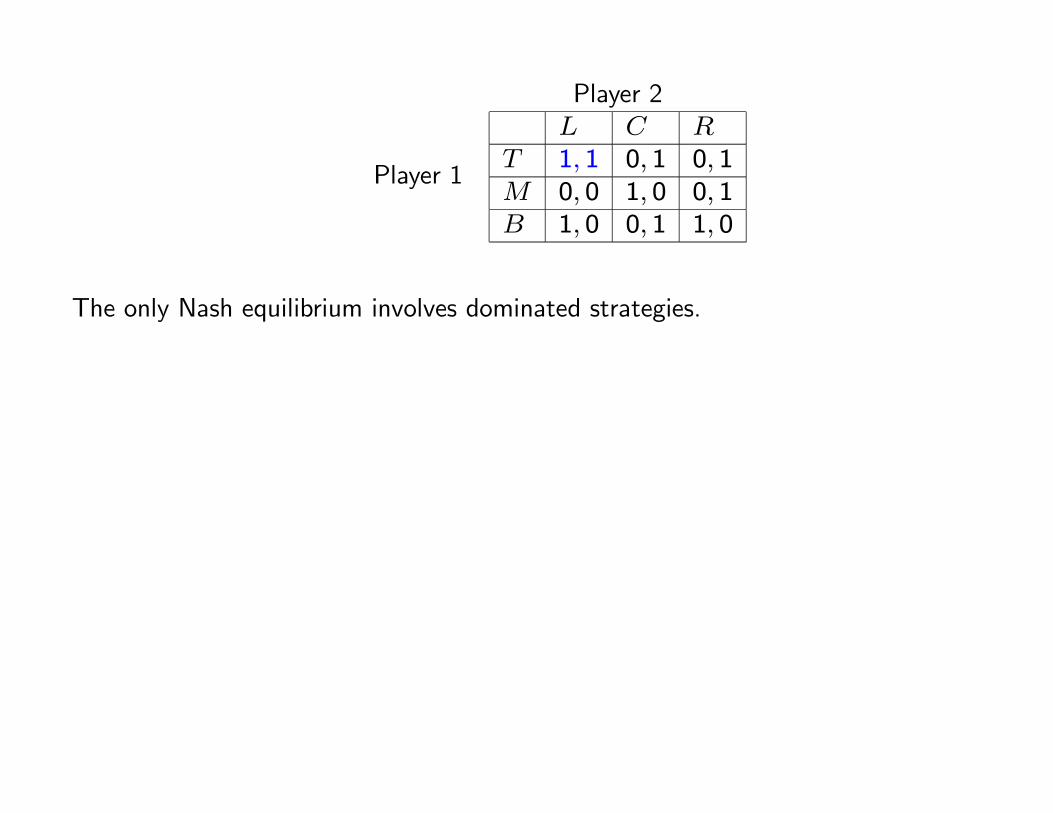
2.3 Nash Equilibrium is not always Plausible
Player 2
Player 1
L C RT 1, 1 0, 1 0, 1M 0, 0 1, 0 0, 1B 1, 0 0, 1 1, 0
Player 2
Player 1
L C RT 1, 1 0, 1 0, 1M 0, 0 1, 0 0, 1B 1, 0 0, 1 1, 0
The only Nash equilibrium involves dominated strategies.
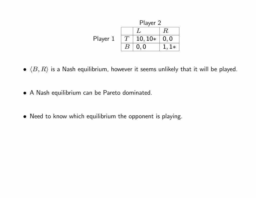
Player 2
Player 1L R
T 10, 10∗ 0, 0B 0, 0 1, 1∗
• 〈B,R〉 is a Nash equilibrium, however it seems unlikely that it will be played.
• A Nash equilibrium can be Pareto dominated.
• Need to know which equilibrium the opponent is playing.
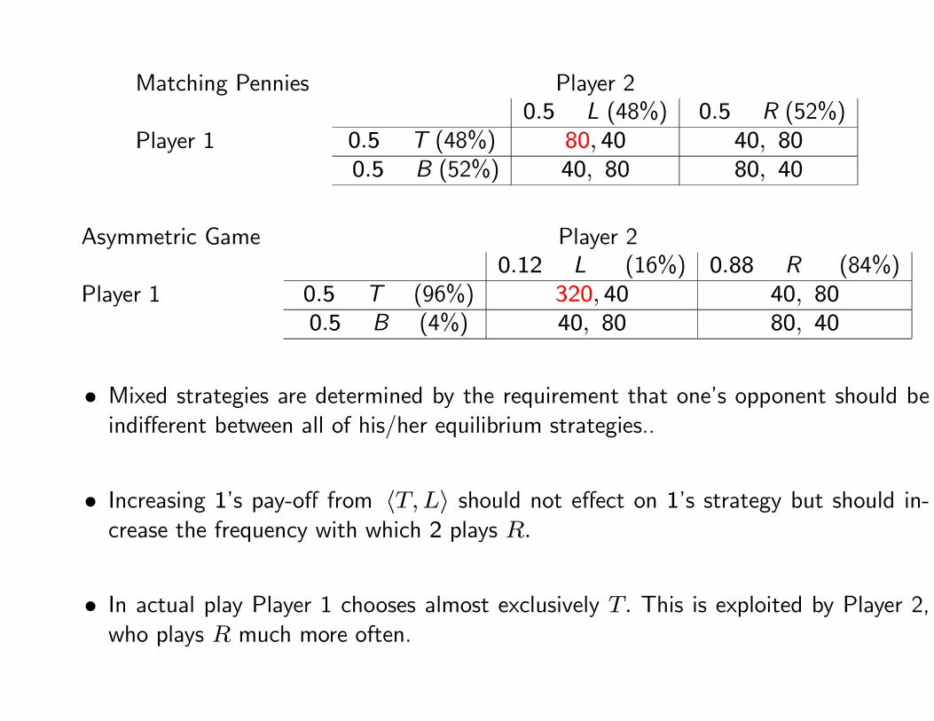
Matching Pennies Player 2
Player 10.5 L (48%) 0.5 R (52%)
0.5 T (48%) 80, 40 40, 800.5 B (52%) 40, 80 80, 40
Asymmetric Game Player 2
Player 10.12 L (16%) 0.88 R (84%)
0.5 T (96%) 320, 40 40, 800.5 B (4%) 40, 80 80, 40
• Mixed strategies are determined by the requirement that one’s opponent should be
indifferent between all of his/her equilibrium strategies..
• Increasing 1’s pay-off from 〈T,L〉 should not effect on 1’s strategy but should in-
crease the frequency with which 2 plays R.
• In actual play Player 1 chooses almost exclusively T. This is exploited by Player 2,
who plays R much more often.
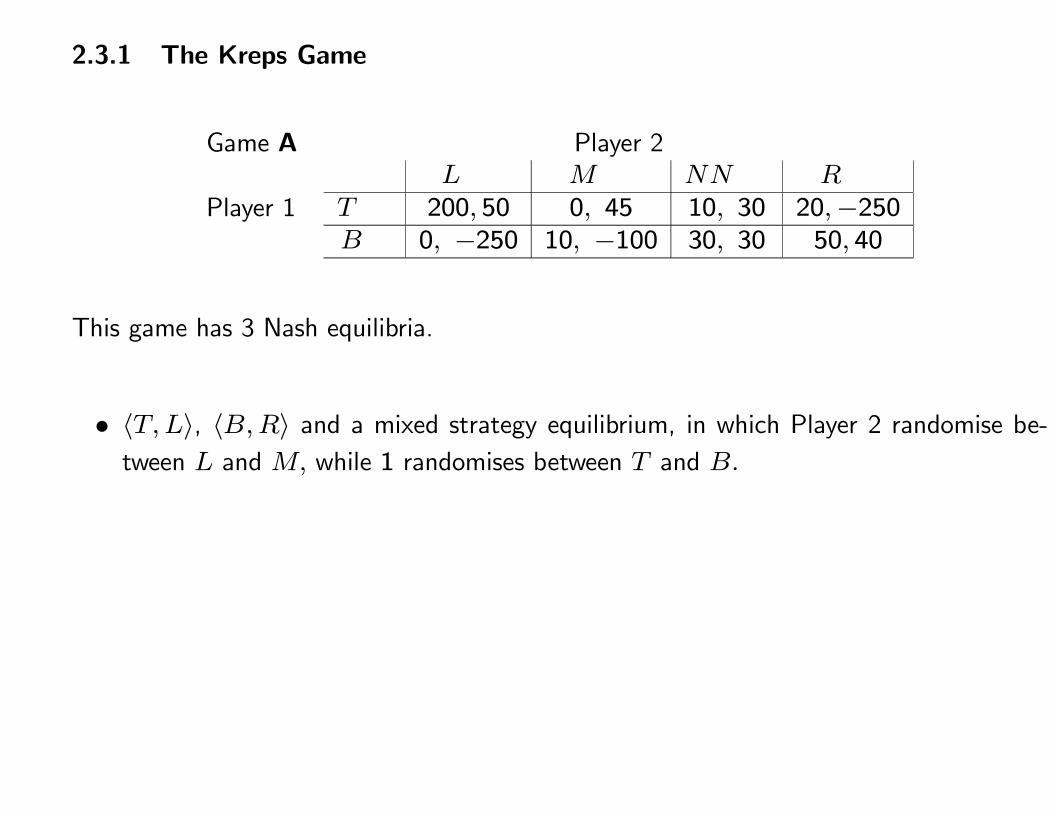
2.3.1 The Kreps Game
Game A Player 2
Player 1L M NN R
T 200, 50 0, 45 10, 30 20,−250B 0, −250 10, −100 30, 30 50, 40
This game has 3 Nash equilibria.
• 〈T,L〉, 〈B,R〉 and a mixed strategy equilibrium, in which Player 2 randomise be-
tween L and M, while 1 randomises between T and B.
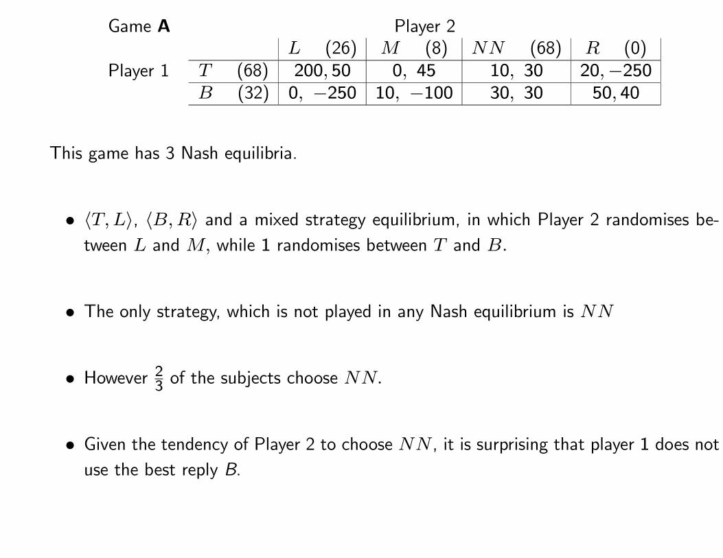
Game A Player 2
Player 1L (26) M (8) NN (68) R (0)
T (68) 200, 50 0, 45 10, 30 20,−250B (32) 0, −250 10, −100 30, 30 50, 40
This game has 3 Nash equilibria.
• 〈T,L〉, 〈B,R〉 and a mixed strategy equilibrium, in which Player 2 randomises be-
tween L and M, while 1 randomises between T and B.
• The only strategy, which is not played in any Nash equilibrium is NN
• However 23 of the subjects choose NN.
• Given the tendency of Player 2 to choose NN , it is surprising that player 1 does not
use the best reply B.
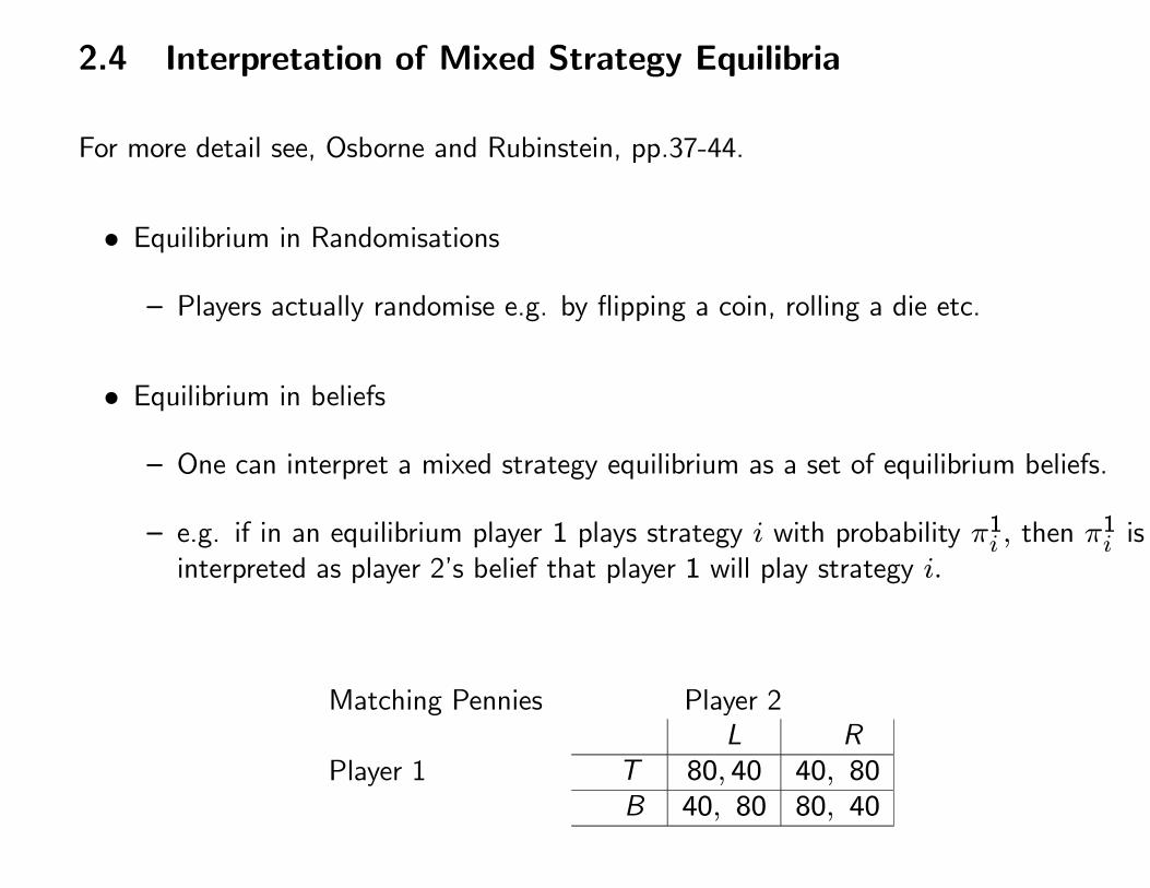
2.4 Interpretation of Mixed Strategy Equilibria
For more detail see, Osborne and Rubinstein, pp.37-44.
• Equilibrium in Randomisations
— Players actually randomise e.g. by flipping a coin, rolling a die etc.
• Equilibrium in beliefs
— One can interpret a mixed strategy equilibrium as a set of equilibrium beliefs.
— e.g. if in an equilibrium player 1 plays strategy i with probability π1i , then π1i is
interpreted as player 2’s belief that player 1 will play strategy i.
Matching Pennies Player 2
Player 1L R
T 80, 40 40, 80B 40, 80 80, 40
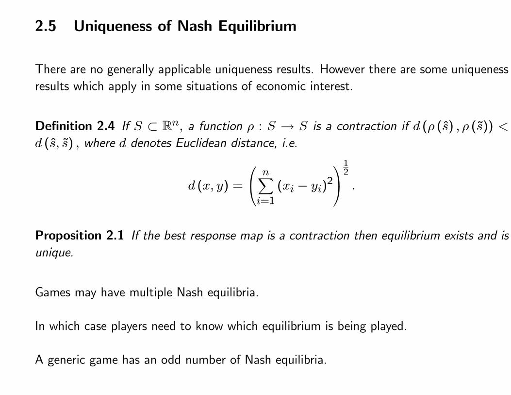
2.5 Uniqueness of Nash Equilibrium
There are no generally applicable uniqueness results. However there are some uniqueness
results which apply in some situations of economic interest.
Definition 2.4 If S ⊂ Rn, a function ρ : S → S is a contraction if d (ρ (s) , ρ (s)) <
d (s, s) , where d denotes Euclidean distance, i.e.
d (x, y) =
n∑
i=1
(xi − yi)2
12
.
Proposition 2.1 If the best response map is a contraction then equilibrium exists and is
unique.
Games may have multiple Nash equilibria.
In which case players need to know which equilibrium is being played.
A generic game has an odd number of Nash equilibria.
2.6 Motivation for Nash Equilibrium
• Stability
— If a proposed solution is not a Nash equilibrium, then at least one party has an
incentive to deviate.
• A non-binding agreement.
• The result of a process of repeated play with similar opponents.
— Cannot be the same opponent since the Nash equilibrium of repeated play with
the same opponent is different to the Nash equilibrium of the one shot game.
• Biological Applications: Evolutionary Stable States.
• Outcome of a ‘learning’ process.
2.7 Criticisms of Nash Equilibria
• In general it may be too complex to calculate Nash equilibria.
— Computers are unable to find Nash equilibria in polynomial time.
• Games may have multiple Nash equilibria.
— In which case players need to know which equilibrium is being played.
• In mixed strategy Nash equilibria players are indifferent between any of the strategies
which they play with positive probability.
— Thus they have no strict incentive to follow the equilibrium strategy.
2.8 Existence of Pure Strategy Nash Equilibria
Mixed strategy Nash equilibria are problematic.
Pure strategy Nash equilibria do not exist in general but do exist for the following important
classes of games.
• Where the strategy space is a closed bounded interval of real numbers;
— or more generally a closed convex and bounded subset of Rn.
• Dominance Solvable games.
• Extensive form games with complete and perfect information.
• Games with strategic complementarity.

THIS WEEK
1. Dominant Strategies (Conclusion)
2. Incomplete Information
3. Problems.
Course website: http://people.exeter.ac.uk/dk210/gt-12.html
DOMINANT STRATEGIES (CONCLUSION)
Existence
One problem with using iterated dominance as a solution concept is that there are relatively
few general existence results. The following are the only reasonably general results which
can be obtained.
A game has strategic complements if there is an ordering on the strategy space and
when one player increases his/her strategy this gives an incentive for his/her rivals to also
increase their strategies.
For example Bertrand Oligopoly.
Theorem 2.2 Let Γ be a game of strategic complements then then set of strategies
remaining after iterated deletion of dominated strategies lie between the highest and
lowest Nash equilibrium.
If Nash equilibrium is unique then it is also an iterated dominance equilibrium.
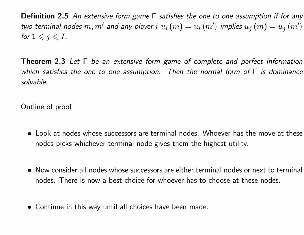
Definition 2.5 An extensive form game Γ satisfies the one to one assumption if for any
two terminal nodes m,m′ and any player i ui (m) = ui(m′)
implies uj (m) = uj(m′)
for 1 � j � I.
Theorem 2.3 Let Γ be an extensive form game of complete and perfect information
which satisfies the one to one assumption. Then the normal form of Γ is dominance
solvable.
Outline of proof
• Look at nodes whose successors are terminal nodes. Whoever has the move at these
nodes picks whichever terminal node gives them the highest utility.
• Now consider all nodes whose successors are either terminal nodes or next to terminal
nodes. There is now a best choice for whoever has to choose at these nodes.
• Continue in this way until all choices have been made.
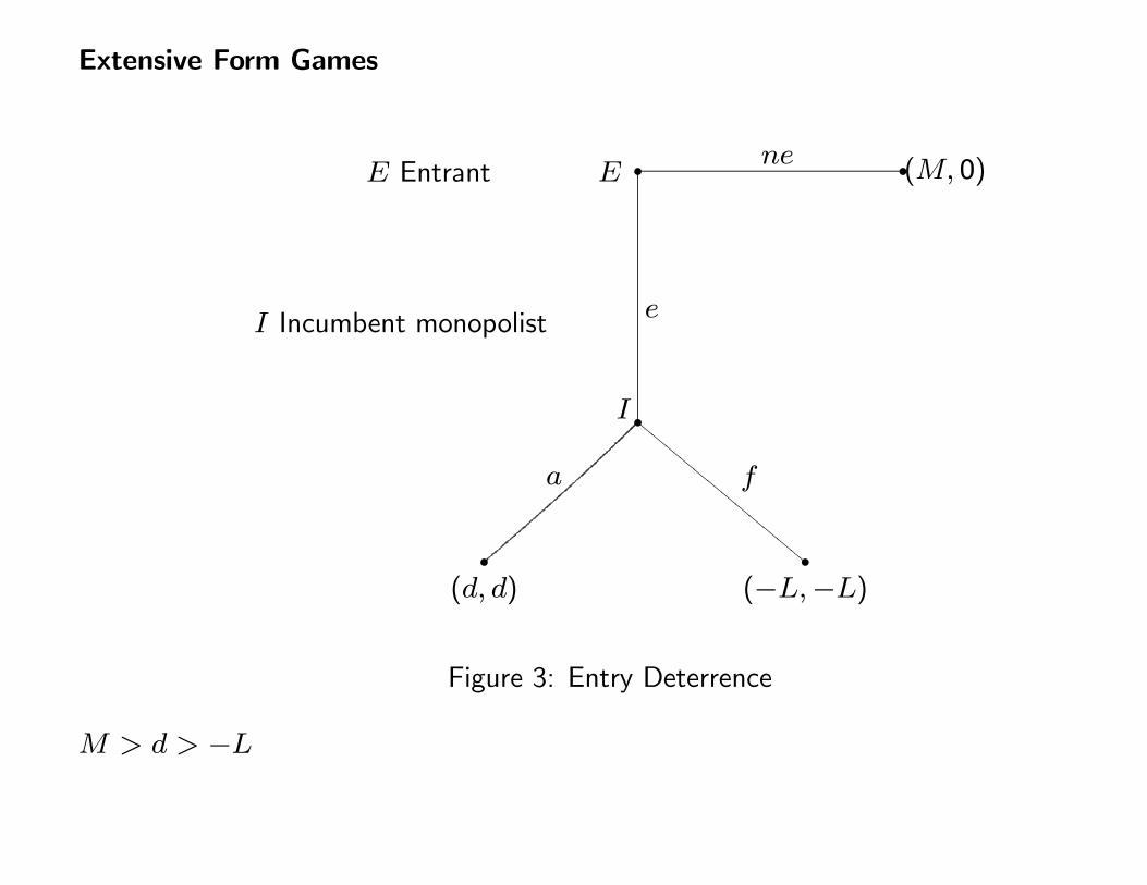
Extensive Form Games
��
�
�
�������������
(M, 0)
(d, d) (−L,−L)
ne
e
a f
I
EE Entrant
I Incumbent monopolist
Figure 3: Entry Deterrence
M > d > −L

Entrant
Incumbente ne
a d, d M, 0f −L,−L M, 0
M > d > −L

�
��
�
�
�
�
� � �
� �
��
�
�
�
�
�� �
�
��
�
�
��
1,1 0,3 2,2 98,98 97,100 99,99 98,101
100,1001 2 1 2121
� � �
D D D D D D D
A A A AAA
Figure 4: Centipede
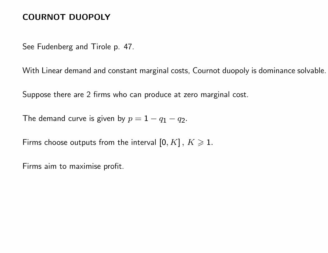
COURNOT DUOPOLY
See Fudenberg and Tirole p. 47.
With Linear demand and constant marginal costs, Cournot duopoly is dominance solvable.
Suppose there are 2 firms who can produce at zero marginal cost.
The demand curve is given by p = 1− q1 − q2.
Firms choose outputs from the interval [0,K] , K � 1.
Firms aim to maximise profit.
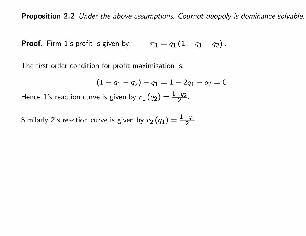
Proposition 2.2 Under the above assumptions, Cournot duopoly is dominance solvable.
Proof. Firm 1’s profit is given by: π1 = q1 (1− q1 − q2) .
The first order condition for profit maximisation is:
(1− q1 − q2)− q1 = 1− 2q1 − q2 = 0.
Hence 1’s reaction curve is given by r1 (q2) =1−q22 .
Similarly 2’s reaction curve is given by r2 (q1) =1−q12 .
The monopoly output is 12. Any strategy in the interval(12,K
]is dominated by 12.
Thus firm 1 knows that firm 2 will not produce in the interval(12,K
].
Given this, all outputs in the range[0, r1
(12
))=[0, 14
)are dominated for firm 1.
(14 is a best response to 12).
If firm 1 does not play strategies the range[0, 14
)all strategies in the interval
(r2(r1(12
)),K
(38,K
]are dominated for firm 2.
Proceeding in this way we can eliminate all strategies except 13 for each firm.

Extensions
• Whenever demand is linear and marginal cost is constant Cournot duopoly is domi-
nance solvable.
• If there are multiple equilibria, Cournot oligopoly is not dominance solvable.
• If there are 3 (or more) firms, Cournot oligopoly is not dominance solvable.
3 GAMES OF INCOMPLETE INFORMATION
3.1 Introduction
References
• Eichberger Ch. 5.
• Kreps, D., A Course in Microeconomic Theory, Harvester Wheatsheaf, 1990,Ch. 13.
• Fudenberg and Tirole, Game Theory. MIT Press 1991, Ch. 6.
Incomplete information Do not know the pay-offs of other players.
Imperfect information Do not know past moves of other players and or nature.
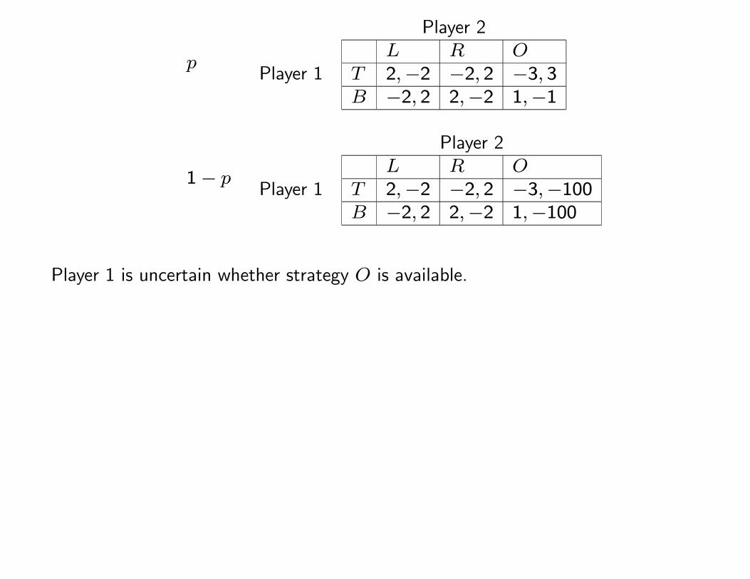
p
Player 2
Player 1L R O
T 2,−2 −2, 2 −3, 3B −2, 2 2,−2 1,−1
1− p
Player 2
Player 1L R O
T 2,−2 −2, 2 −3,−100B −2, 2 2,−2 1,−100
Player 1 is uncertain whether strategy O is available.
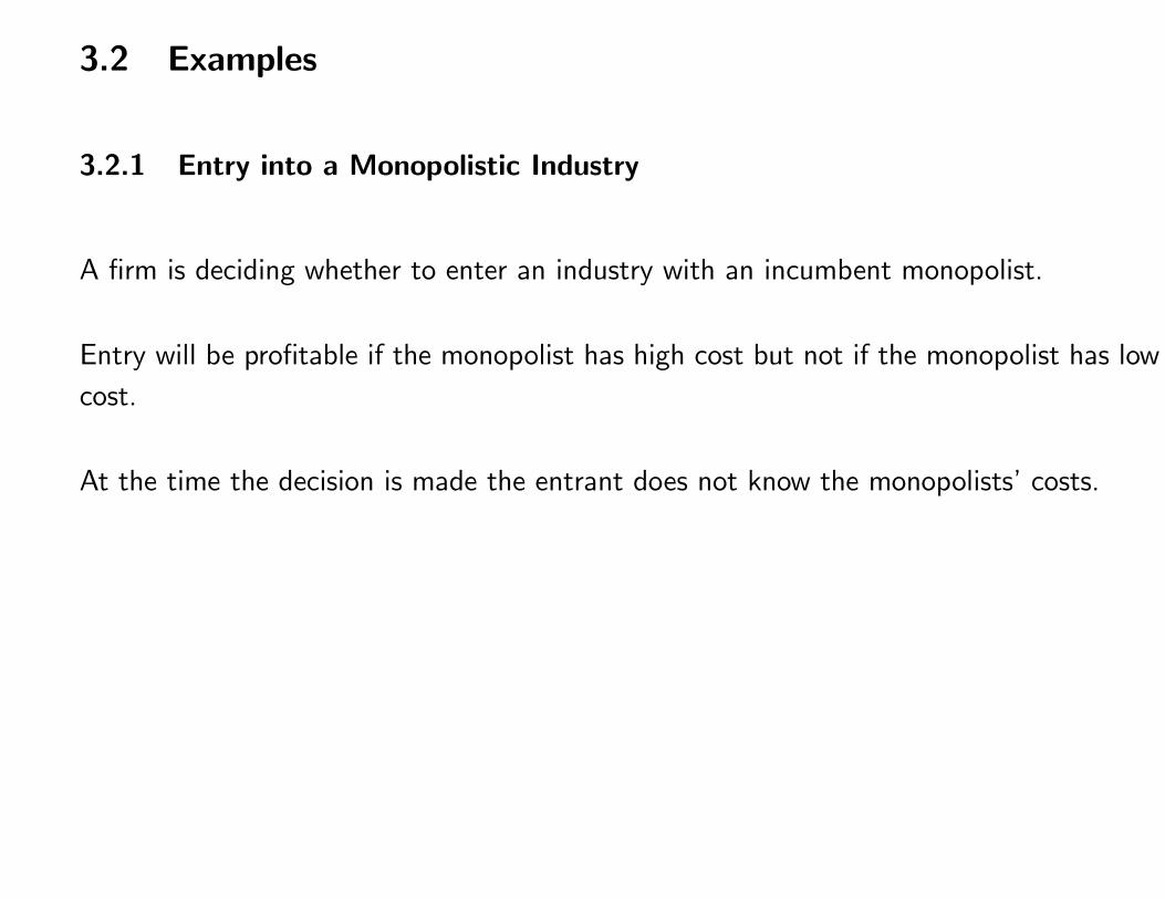
3.2 Examples
3.2.1 Entry into a Monopolistic Industry
A firm is deciding whether to enter an industry with an incumbent monopolist.
Entry will be profitable if the monopolist has high cost but not if the monopolist has low
cost.
At the time the decision is made the entrant does not know the monopolists’ costs.
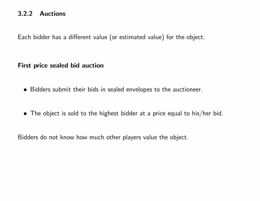
3.2.2 Auctions
Each bidder has a different value (or estimated value) for the object.
First price sealed bid auction
• Bidders submit their bids in sealed envelopes to the auctioneer.
• The object is sold to the highest bidder at a price equal to his/her bid.
Bidders do not know how much other players value the object.
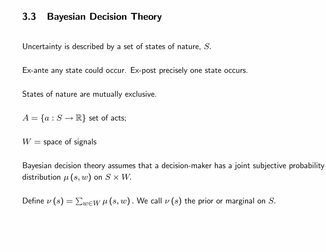
3.3 Bayesian Decision Theory
Uncertainty is described by a set of states of nature, S.
Ex-ante any state could occur. Ex-post precisely one state occurs.
States of nature are mutually exclusive.
A = {a : S → R} set of acts;
W = space of signals
Bayesian decision theory assumes that a decision-maker has a joint subjective probability
distribution µ (s,w) on S ×W.
Define ν (s) =∑w∈W µ (s,w) . We call ν (s) the prior or marginal on S.
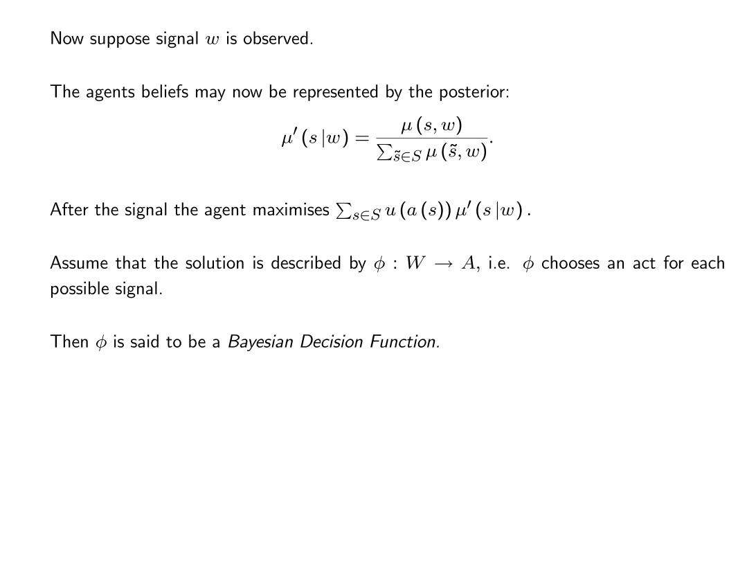
Now suppose signal w is observed.
The agents beliefs may now be represented by the posterior:
µ′ (s |w) =µ (s,w)
∑s∈S µ (s, w)
.
After the signal the agent maximises∑s∈S u (a (s))µ
′ (s |w) .
Assume that the solution is described by φ : W → A, i.e. φ chooses an act for each
possible signal.
Then φ is said to be a Bayesian Decision Function.
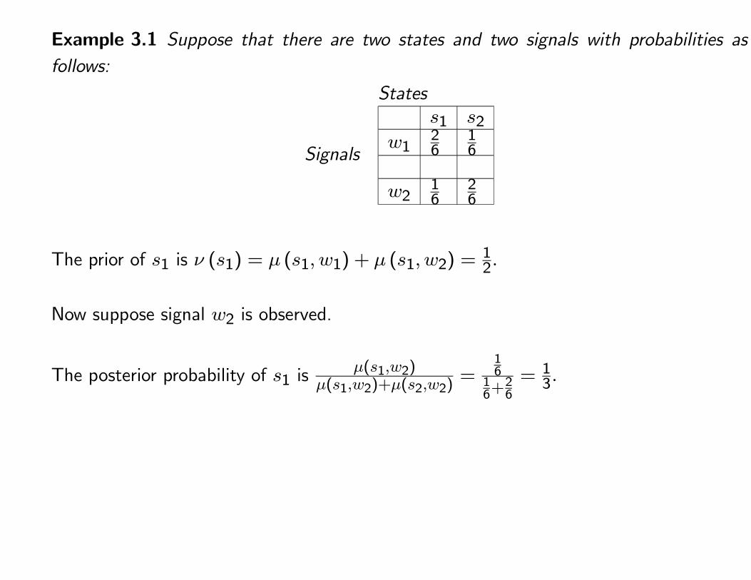
Example 3.1 Suppose that there are two states and two signals with probabilities as
follows:
States
Signals
s1 s2w1
26
16
w216
26
The prior of s1 is ν (s1) = µ (s1, w1) + µ (s1, w2) =12.
Now suppose signal w2 is observed.
The posterior probability of s1 isµ(s1,w2)
µ(s1,w2)+µ(s2,w2)=
1616+26
= 13.
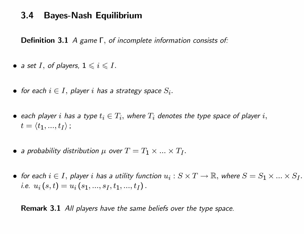
3.4 Bayes-Nash Equilibrium
Definition 3.1 A game Γ, of incomplete information consists of:
• a set I, of players, 1 � i � I.
• for each i ∈ I, player i has a strategy space Si.
• each player i has a type ti ∈ Ti, where Ti denotes the type space of player i,
t = 〈t1, ..., tI〉 ;
• a probability distribution µ over T = T1 × ...× TI.
• for each i ∈ I, player i has a utility function ui : S×T → R, where S = S1× ...×SI.
i.e. ui (s, t) = ui (s1, ..., sI, t1, ..., tI) .
Remark 3.1 All players have the same beliefs over the type space.
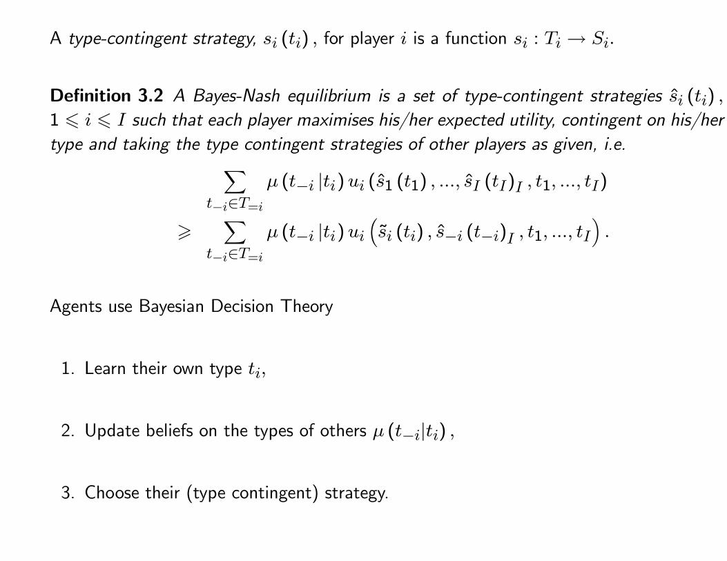
A type-contingent strategy, si (ti) , for player i is a function si : Ti→ Si.
Definition 3.2 A Bayes-Nash equilibrium is a set of type-contingent strategies si (ti) ,
1 � i � I such that each player maximises his/her expected utility, contingent on his/her
type and taking the type contingent strategies of other players as given, i.e.∑
t−i∈T=i
µ (t−i |ti)ui (s1 (t1) , ..., sI (tI)I , t1, ..., tI)
�∑
t−i∈T=i
µ (t−i |ti)ui(si (ti) , s−i (t−i)I , t1, ..., tI
).
Agents use Bayesian Decision Theory
1. Learn their own type ti,
2. Update beliefs on the types of others µ (t−i|ti) ,
3. Choose their (type contingent) strategy.
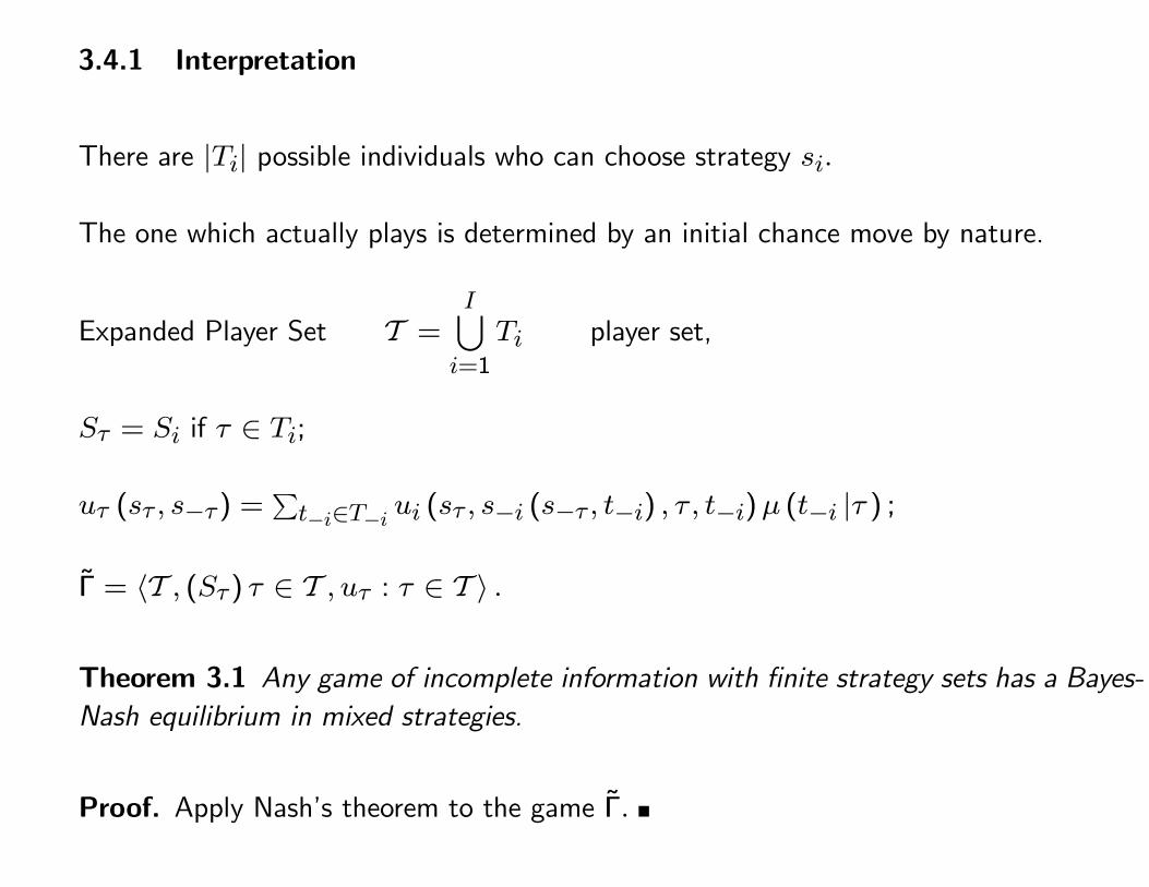
3.4.1 Interpretation
There are |Ti| possible individuals who can choose strategy si.
The one which actually plays is determined by an initial chance move by nature.
Expanded Player Set T =I⋃
i=1
Ti player set,
Sτ = Si if τ ∈ Ti;
uτ (sτ , s−τ) =∑t−i∈T−i ui (sτ , s−i (s−τ , t−i) , τ , t−i)µ (t−i |τ ) ;
Γ = 〈T , (Sτ) τ ∈ T , uτ : τ ∈ T 〉 .
Theorem 3.1 Any game of incomplete information with finite strategy sets has a Bayes-
Nash equilibrium in mixed strategies.
Proof. Apply Nash’s theorem to the game Γ.
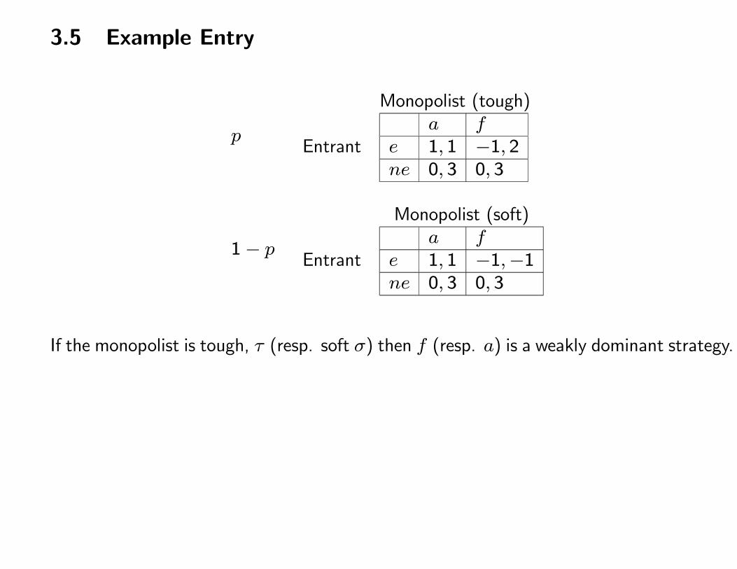
3.5 Example Entry
p
Monopolist (tough)
Entranta f
e 1, 1 −1, 2ne 0, 3 0, 3
1− p
Monopolist (soft)
Entranta f
e 1, 1 −1,−1ne 0, 3 0, 3
If the monopolist is tough, τ (resp. soft σ) then f (resp. a) is a weakly dominant strategy.
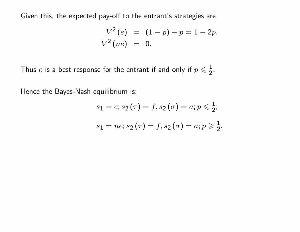
Given this, the expected pay-off to the entrant’s strategies are
V 2 (e) = (1− p)− p = 1− 2p.
V 2 (ne) = 0.
Thus e is a best response for the entrant if and only if p � 12.
Hence the Bayes-Nash equilibrium is:
s1 = e; s2 (τ) = f, s2 (σ) = a; p �12;
s1 = ne; s2 (τ) = f, s2 (σ) = a; p �12.
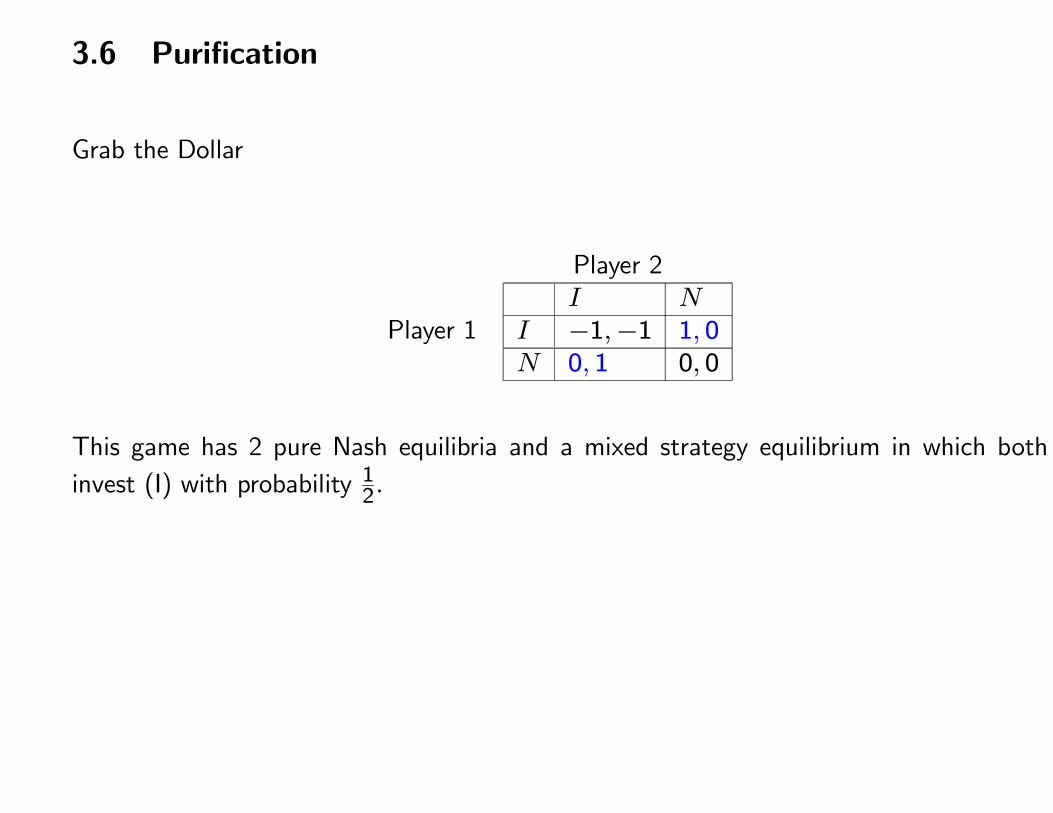
3.6 Purification
Grab the Dollar
Player 2
Player 1I N
I −1,−1 1, 0N 0, 1 0, 0
This game has 2 pure Nash equilibria and a mixed strategy equilibrium in which both
invest (I) with probability 12.
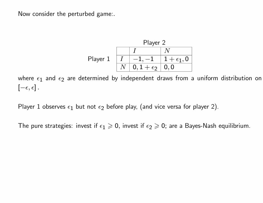
Now consider the perturbed game:.
Player 2
Player 1I N
I −1,−1 1 + ǫ1, 0N 0, 1 + ǫ2 0, 0
where ǫ1 and ǫ2 are determined by independent draws from a uniform distribution on
[−ǫ, ǫ] .
Player 1 observes ǫ1 but not ǫ2 before play, (and vice versa for player 2).
The pure strategies: invest if ǫ1 � 0, invest if ǫ2 � 0; are a Bayes-Nash equilibrium.
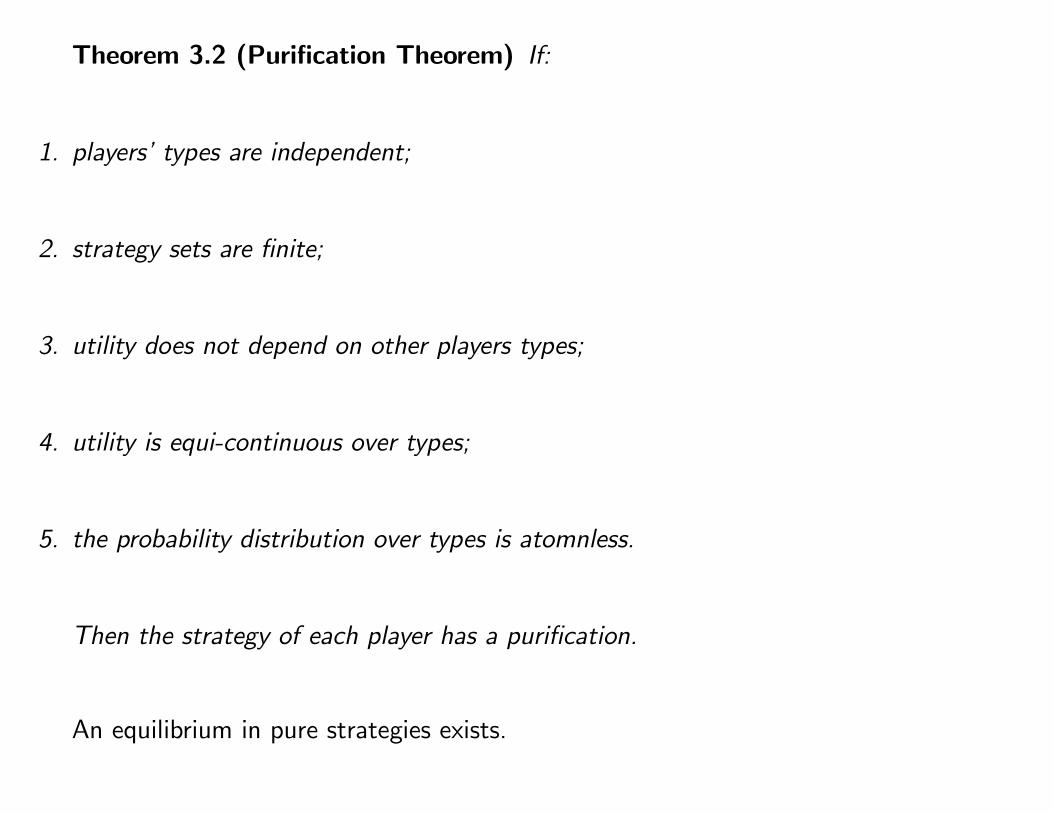
Theorem 3.2 (Purification Theorem) If:
1. players’ types are independent;
2. strategy sets are finite;
3. utility does not depend on other players types;
4. utility is equi-continuous over types;
5. the probability distribution over types is atomnless.
Then the strategy of each player has a purification.
An equilibrium in pure strategies exists.
3.7 Applications
3.7.1 Chain Store Paradox
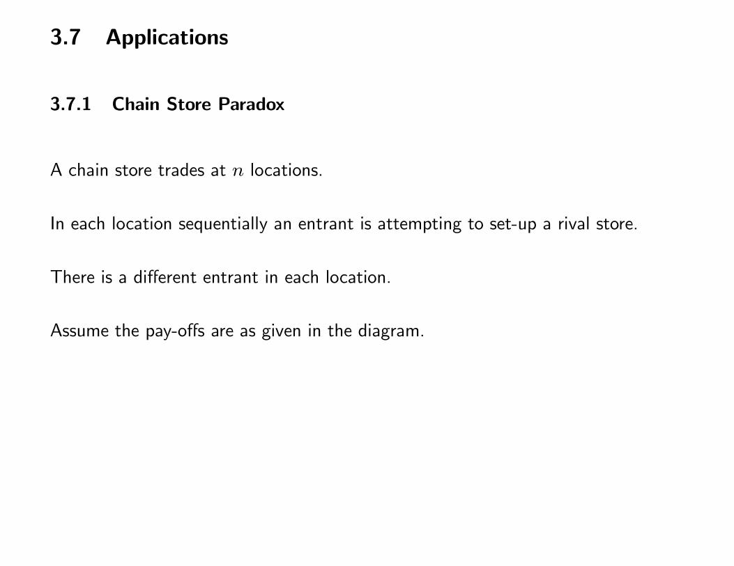
A chain store trades at n locations.
In each location sequentially an entrant is attempting to set-up a rival store.
There is a different entrant in each location.
Assume the pay-offs are as given in the diagram.
��
�
�
������������
(3, 0)
(0, 4) (−4,−4)
ne
e
a f
I
E1
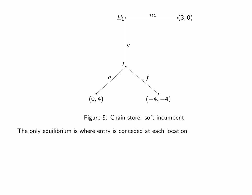
Figure 5: Chain store: soft incumbent
The only equilibrium is where entry is conceded at each location.
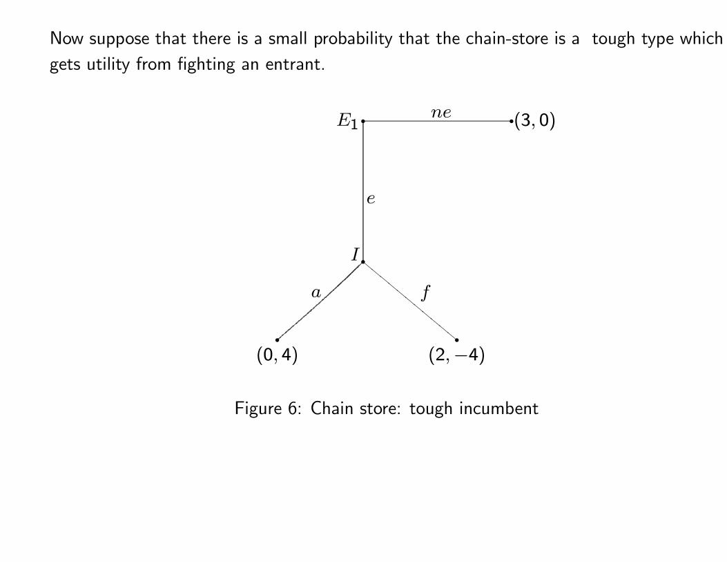
Now suppose that there is a small probability that the chain-store is a tough type which
gets utility from fighting an entrant.
��
�
�
������������
(3, 0)
(0, 4) (2,−4)
ne
e
a f
I
E1
Figure 6: Chain store: tough incumbent
In this case there is an equilibrium where the chain-store always fights the initial entrants.
i.e. even the soft type fights.
This allows it to acquire a reputation for being tough and thus deters future entrants.
The first entrant stays out if π < 12n−1
, where π is the prior probability that the incumbent
is tough.
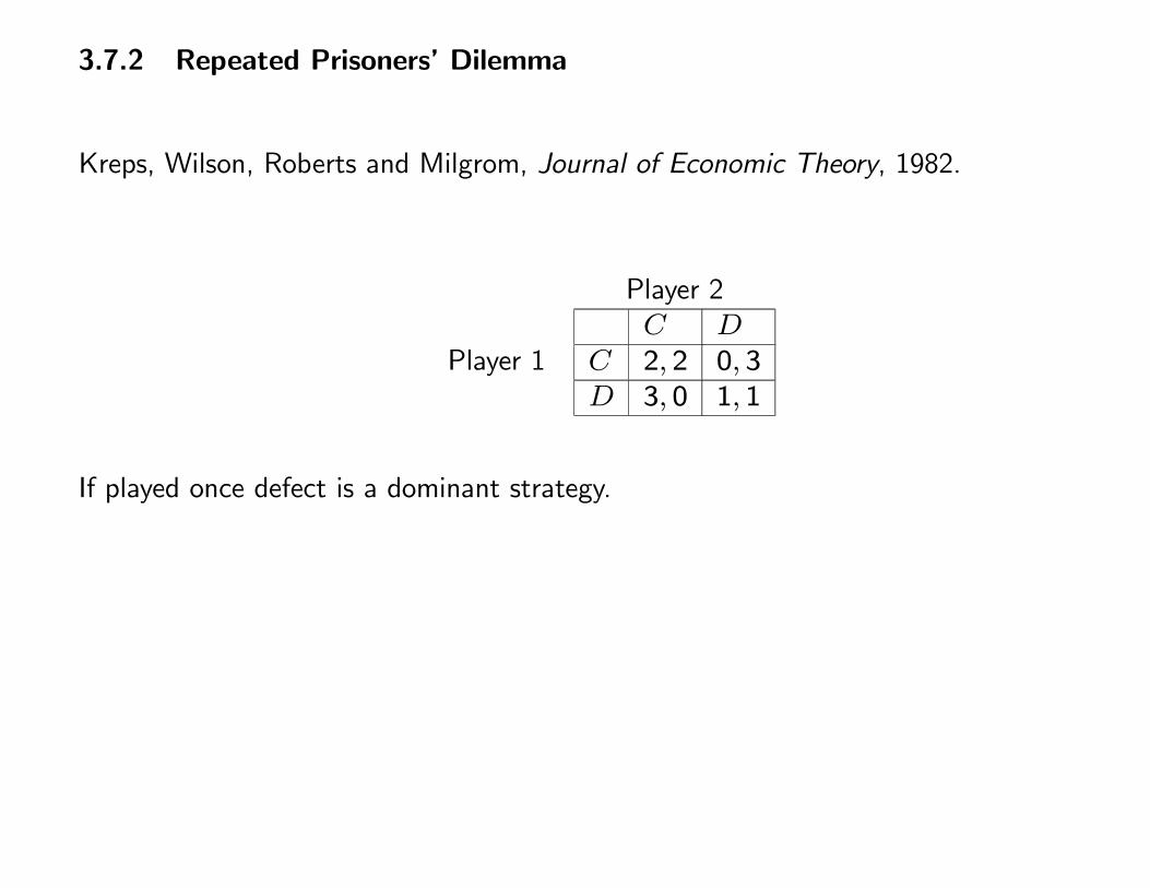
3.7.2 Repeated Prisoners’ Dilemma
Kreps, Wilson, Roberts and Milgrom, Journal of Economic Theory, 1982.
Player 2
Player 1C D
C 2, 2 0, 3D 3, 0 1, 1
If played once defect is a dominant strategy.
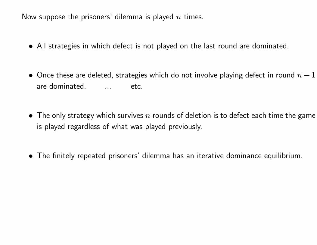
Now suppose the prisoners’ dilemma is played n times.
• All strategies in which defect is not played on the last round are dominated.
• Once these are deleted, strategies which do not involve playing defect in round n−1
are dominated. ... etc.
• The only strategy which survives n rounds of deletion is to defect each time the game
is played regardless of what was played previously.
• The finitely repeated prisoners’ dilemma has an iterative dominance equilibrium.
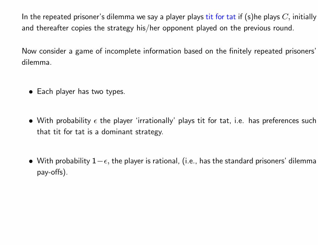
In the repeated prisoner’s dilemma we say a player plays tit for tat if (s)he plays C, initially
and thereafter copies the strategy his/her opponent played on the previous round.
Now consider a game of incomplete information based on the finitely repeated prisoners’
dilemma.
• Each player has two types.
• With probability ǫ the player ‘irrationally’ plays tit for tat, i.e. has preferences such
that tit for tat is a dominant strategy.
• With probability 1−ǫ, the player is rational, (i.e., has the standard prisoners’ dilemma
pay-offs).
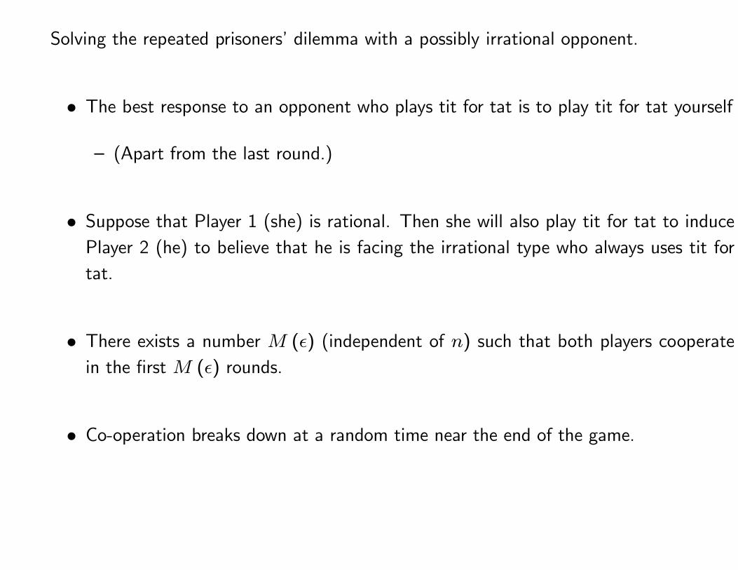
Solving the repeated prisoners’ dilemma with a possibly irrational opponent.
• The best response to an opponent who plays tit for tat is to play tit for tat yourself
— (Apart from the last round.)
• Suppose that Player 1 (she) is rational. Then she will also play tit for tat to induce
Player 2 (he) to believe that he is facing the irrational type who always uses tit for
tat.
• There exists a number M (ǫ) (independent of n) such that both players cooperate
in the first M (ǫ) rounds.
• Co-operation breaks down at a random time near the end of the game.
Suppose instead there is a small probability that the opponent has an irrational type who
always cooperates.
• Then the only equilibrium in the finitely repeated prisoners’ dilemma is to defect at
each stage.
Thus the outcome depends on the nature of the irrationality, which the irrational type is
assumed to have.
3.8 Conclusion
• Incomplete information has significantly increased the set of situations which can be
modelled as games.
• Major applications include
— Auctions
— The Kreps-Wilson model of predatory pricing/entry deterrence.
• Incomplete information provides a way to model reputation.
• The disadvantage of this approach is that games become more complex and difficult
to solve in practice.
— Adding extra types is equivalent to adding extra players.
Recall in a Game of incomplete information utility depends on a player’s type as well as
his/her strategy.
Types are assigned randomly by an initial move by nature.

THIS WEEK
1. Repeated Games (Start).
2. Problem Sheet 1
NEXT WEEK
1. Repeated Games (Conclusion)
2. Problem Sheet 2
4 REPEATED GAMES
4.1 Introduction
Suppose two (or more) players play the same game repeatedly.
There is more scope for cooperation since a player who defects now can be “punished”
by lack of cooperation in the future.
Implicit collusion in oligopolistic industries.
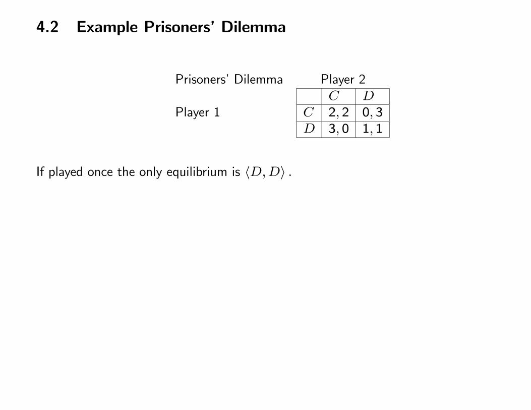
4.2 Example Prisoners’ Dilemma
Prisoners’ Dilemma Player 2
Player 1C D
C 2, 2 0, 3D 3, 0 1, 1
If played once the only equilibrium is 〈D,D〉 .
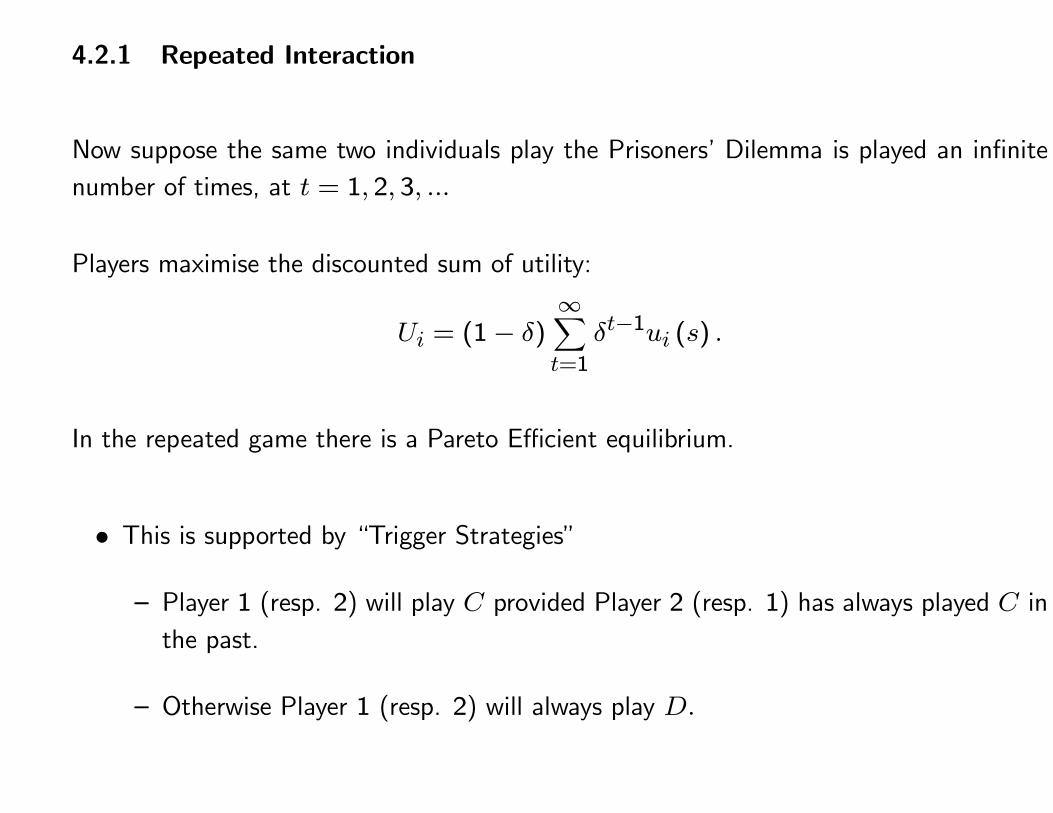
4.2.1 Repeated Interaction
Now suppose the same two individuals play the Prisoners’ Dilemma is played an infinite
number of times, at t = 1, 2, 3, ...
Players maximise the discounted sum of utility:
Ui = (1− δ)∞∑
t=1
δt−1ui (s) .
In the repeated game there is a Pareto Efficient equilibrium.
• This is supported by “Trigger Strategies”
— Player 1 (resp. 2) will play C provided Player 2 (resp. 1) has always played C in
the past.
— Otherwise Player 1 (resp. 2) will always play D.
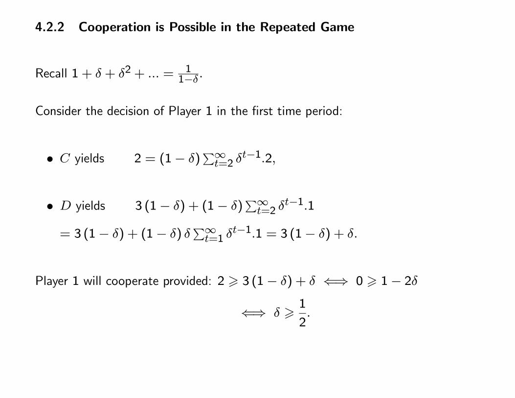
4.2.2 Cooperation is Possible in the Repeated Game
Recall 1 + δ + δ2 + ... = 11−δ.
Consider the decision of Player 1 in the first time period:
• C yields 2 = (1− δ)∑∞t=2 δ
t−1.2,
• D yields 3 (1− δ) + (1− δ)∑∞t=2 δ
t−1.1
= 3 (1− δ) + (1− δ) δ∑∞t=1 δ
t−1.1 = 3 (1− δ) + δ.
Player 1 will cooperate provided: 2 � 3 (1− δ) + δ ⇐⇒ 0 � 1− 2δ
⇐⇒ δ �1
2.
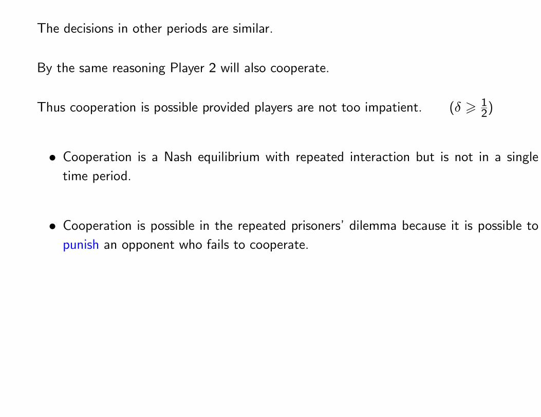
The decisions in other periods are similar.
By the same reasoning Player 2 will also cooperate.
Thus cooperation is possible provided players are not too impatient. (δ � 12)
• Cooperation is a Nash equilibrium with repeated interaction but is not in a single
time period.
• Cooperation is possible in the repeated prisoners’ dilemma because it is possible to
punish an opponent who fails to cooperate.
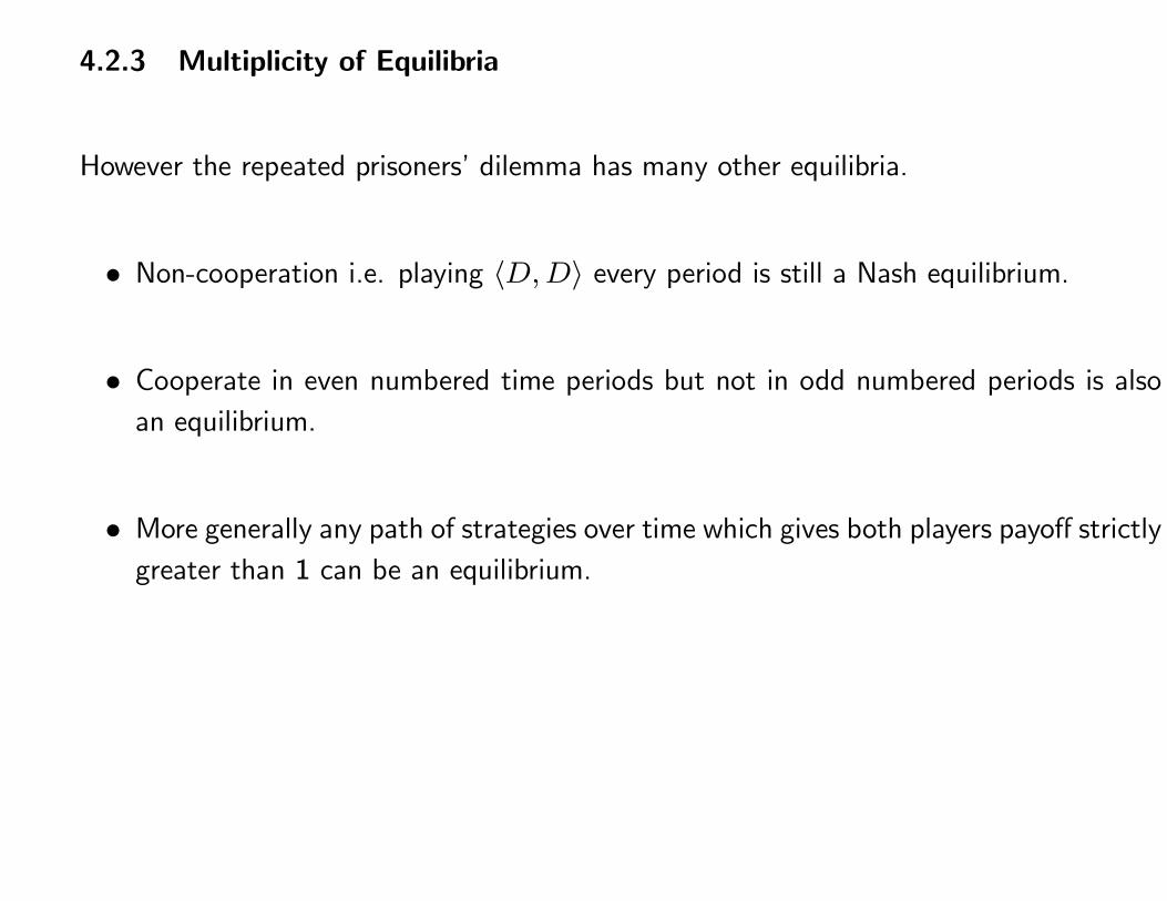
4.2.3 Multiplicity of Equilibria
However the repeated prisoners’ dilemma has many other equilibria.
• Non-cooperation i.e. playing 〈D,D〉 every period is still a Nash equilibrium.
• Cooperate in even numbered time periods but not in odd numbered periods is also
an equilibrium.
• More generally any path of strategies over time which gives both players payoff strictly
greater than 1 can be an equilibrium.
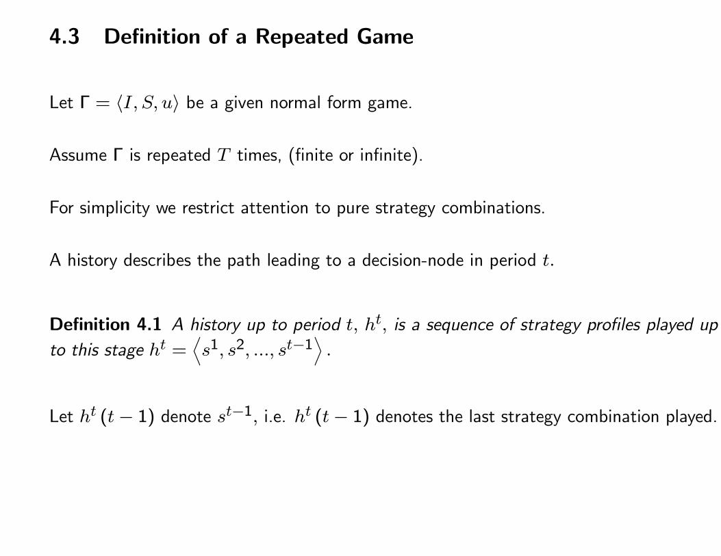
4.3 Definition of a Repeated Game
Let Γ = 〈I, S, u〉 be a given normal form game.
Assume Γ is repeated T times, (finite or infinite).
For simplicity we restrict attention to pure strategy combinations.
A history describes the path leading to a decision-node in period t.
Definition 4.1 A history up to period t, ht, is a sequence of strategy profiles played up
to this stage ht =⟨s1, s2, ..., st−1
⟩.
Let ht (t− 1) denote st−1, i.e. ht (t− 1) denotes the last strategy combination played.
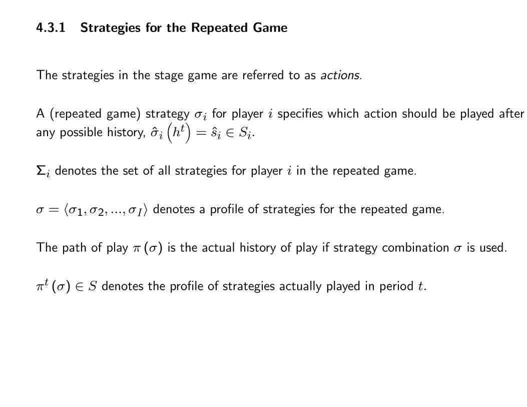
4.3.1 Strategies for the Repeated Game
The strategies in the stage game are referred to as actions.
A (repeated game) strategy σi for player i specifies which action should be played after
any possible history, σi(ht)= si ∈ Si.
Σi denotes the set of all strategies for player i in the repeated game.
σ = 〈σ1, σ2, ..., σI〉 denotes a profile of strategies for the repeated game.
The path of play π (σ) is the actual history of play if strategy combination σ is used.
πt (σ) ∈ S denotes the profile of strategies actually played in period t.
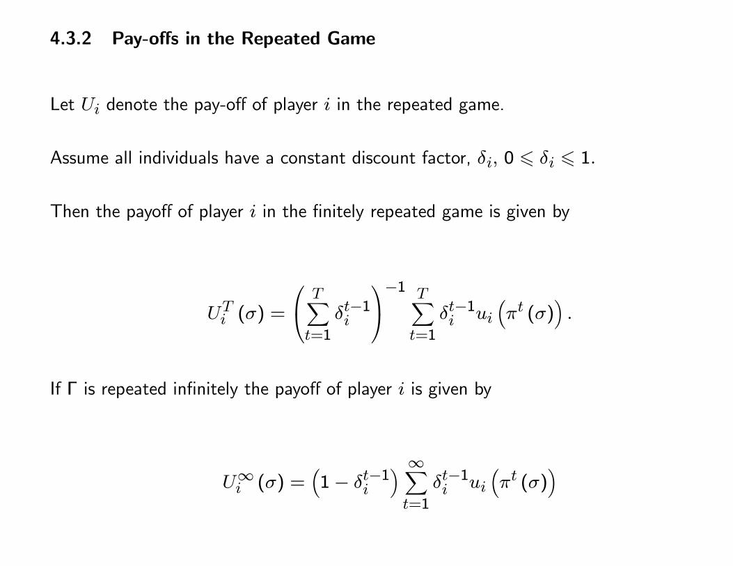
4.3.2 Pay-offs in the Repeated Game
Let Ui denote the pay-off of player i in the repeated game.
Assume all individuals have a constant discount factor, δi, 0 � δi � 1.
Then the payoff of player i in the finitely repeated game is given by
UTi (σ) =
T∑
t=1
δt−1i
−1 T∑
t=1
δt−1i ui(πt (σ)
).
If Γ is repeated infinitely the payoff of player i is given by
U∞i (σ) =(1− δt−1i
) ∞∑
t=1
δt−1i ui(πt (σ)
)
4.3.3 Punishment
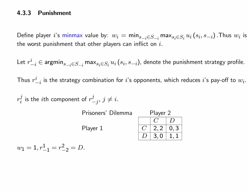
Define player i’s minmax value by: wi = mins−i∈S−imaxsi∈Si ui (si, s−i) .Thus wi is
the worst punishment that other players can inflict on i.
Let ri−i ∈ argmins−i∈S−imaxsi∈Si ui (si, s−i), denote the punishment strategy profile.
Thus ri−i is the strategy combination for i’s opponents, which reduces i’s pay-off to wi.
rji is the ith component of r
j−j, j �= i.
Prisoners’ Dilemma Player 2
Player 1C D
C 2, 2 0, 3D 3, 0 1, 1
w1 = 1, r1−1 = r
2−2 = D.
4.3.4 Individually Rational Pay-offs
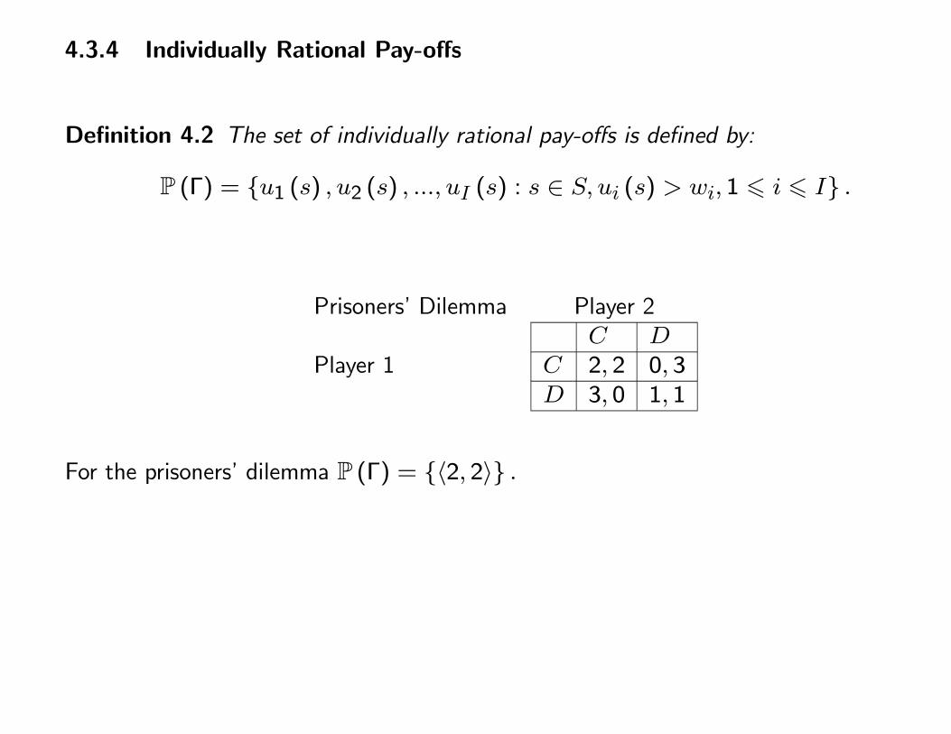
Definition 4.2 The set of individually rational pay-offs is defined by:
P (Γ) = {u1 (s) , u2 (s) , ..., uI (s) : s ∈ S, ui (s) > wi, 1 � i � I} .
Prisoners’ Dilemma Player 2
Player 1C D
C 2, 2 0, 3D 3, 0 1, 1
For the prisoners’ dilemma P (Γ) = {〈2, 2〉} .
4.4 Infinitely Repeated Games
4.4.1 Nash Equilibrium
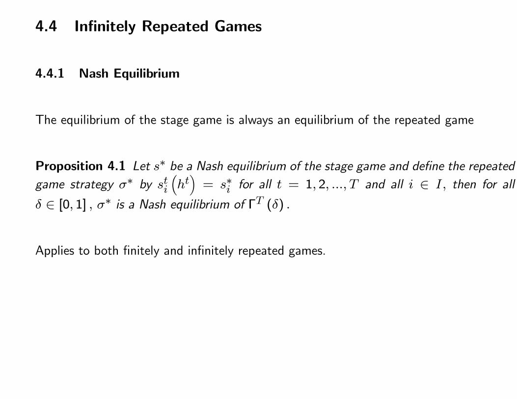
The equilibrium of the stage game is always an equilibrium of the repeated game
Proposition 4.1 Let s∗ be a Nash equilibrium of the stage game and define the repeated
game strategy σ∗ by sti
(ht)= s∗i for all t = 1, 2, ..., T and all i ∈ I, then for all
δ ∈ [0, 1] , σ∗ is a Nash equilibrium of ΓT (δ) .
Applies to both finitely and infinitely repeated games.
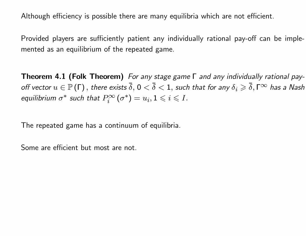
Although efficiency is possible there are many equilibria which are not efficient.
Provided players are sufficiently patient any individually rational pay-off can be imple-
mented as an equilibrium of the repeated game.
Theorem 4.1 (Folk Theorem) For any stage game Γ and any individually rational pay-
off vector u ∈ P (Γ) , there exists δ, 0 < δ < 1, such that for any δi � δ,Γ∞ has a Nash
equilibrium σ∗ such that P∞i (σ∗) = ui, 1 � i � I.
The repeated game has a continuum of equilibria.
Some are efficient but most are not.
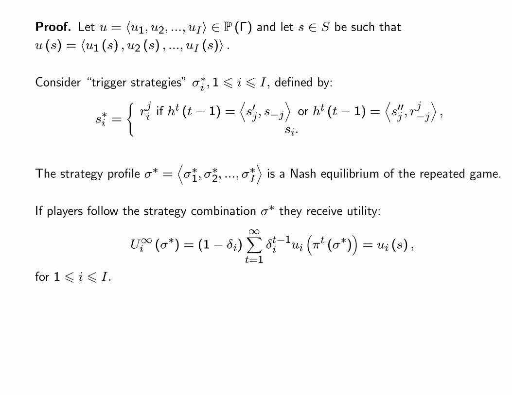
Proof. Let u = 〈u1, u2, ..., uI〉 ∈ P (Γ) and let s ∈ S be such that
u (s) = 〈u1 (s) , u2 (s) , ..., uI (s)〉 .
Consider “trigger strategies” σ∗i , 1 � i � I, defined by:
s∗i =
{rji if ht (t− 1) =
⟨s′j, s−j
⟩or ht (t− 1) =
⟨s′′j , r
j−j
⟩,
si.
The strategy profile σ∗ =⟨σ∗1, σ
∗2, ..., σ
∗I
⟩is a Nash equilibrium of the repeated game.
If players follow the strategy combination σ∗ they receive utility:
U∞i (σ∗) = (1− δi)
∞∑
t=1
δt−1i ui(πt (σ∗)
)= ui (s) ,
for 1 � i � I.
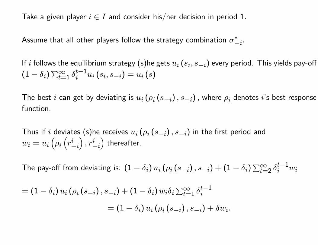
Take a given player i ∈ I and consider his/her decision in period 1.
Assume that all other players follow the strategy combination σ∗−i.
If i follows the equilibrium strategy (s)he gets ui (si, s−i) every period. This yields pay-off
(1− δi)∑∞t=1 δ
t−1i ui (si, s−i) = ui (s)
The best i can get by deviating is ui (ρi (s−i) , s−i) , where ρi denotes i’s best response
function.
Thus if i deviates (s)he receives ui (ρi (s−i) , s−i) in the first period and
wi = ui(ρi(ri−i
), ri−i
)thereafter.
The pay-off from deviating is: (1− δi)ui (ρi (s−i) , s−i) + (1− δi)∑∞t=2 δ
t−1i wi
= (1− δi)ui (ρi (s−i) , s−i) + (1− δi)wiδi∑∞t=1 δ
t−1i
= (1− δi)ui (ρi (s−i) , s−i) + δwi.
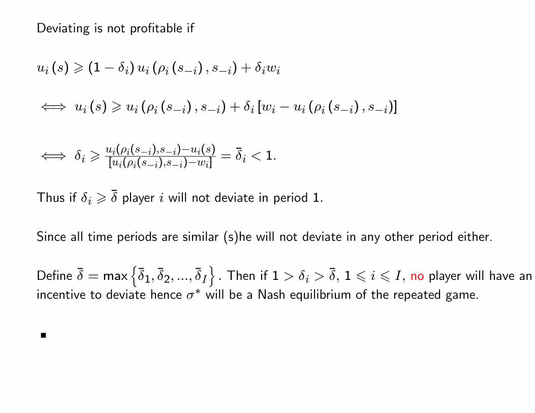
Deviating is not profitable if
ui (s) � (1− δi)ui (ρi (s−i) , s−i) + δiwi
⇐⇒ ui (s) � ui (ρi (s−i) , s−i) + δi [wi − ui (ρi (s−i) , s−i)]
⇐⇒ δi �ui(ρi(s−i),s−i)−ui(s)[ui(ρi(s−i),s−i)−wi]
= δi < 1.
Thus if δi � δ player i will not deviate in period 1.
Since all time periods are similar (s)he will not deviate in any other period either.
Define δ = max{δ1, δ2, ..., δI
}. Then if 1 > δi > δ, 1 � i � I, no player will have an
incentive to deviate hence σ∗ will be a Nash equilibrium of the repeated game.
THIS WEEK
1. Repeated Games (Conclusion)
• Subgame Perfect Equilibria of Infinitely Repeated
2. Problem Sheet 2
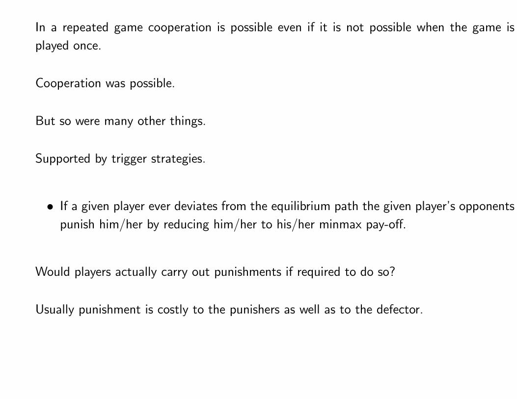
In a repeated game cooperation is possible even if it is not possible when the game is
played once.
Cooperation was possible.
But so were many other things.
Supported by trigger strategies.
• If a given player ever deviates from the equilibrium path the given player’s opponents
punish him/her by reducing him/her to his/her minmax pay-off.
Would players actually carry out punishments if required to do so?
Usually punishment is costly to the punishers as well as to the defector.
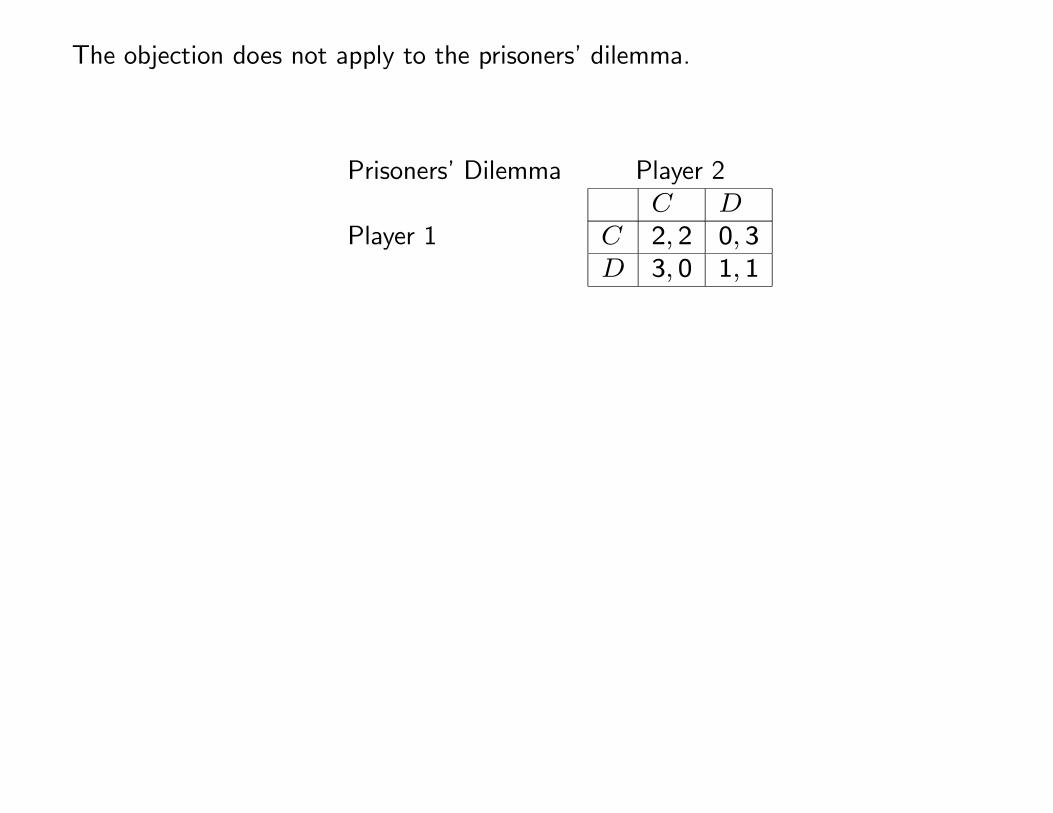
The objection does not apply to the prisoners’ dilemma.
Prisoners’ Dilemma Player 2
Player 1C D
C 2, 2 0, 3D 3, 0 1, 1
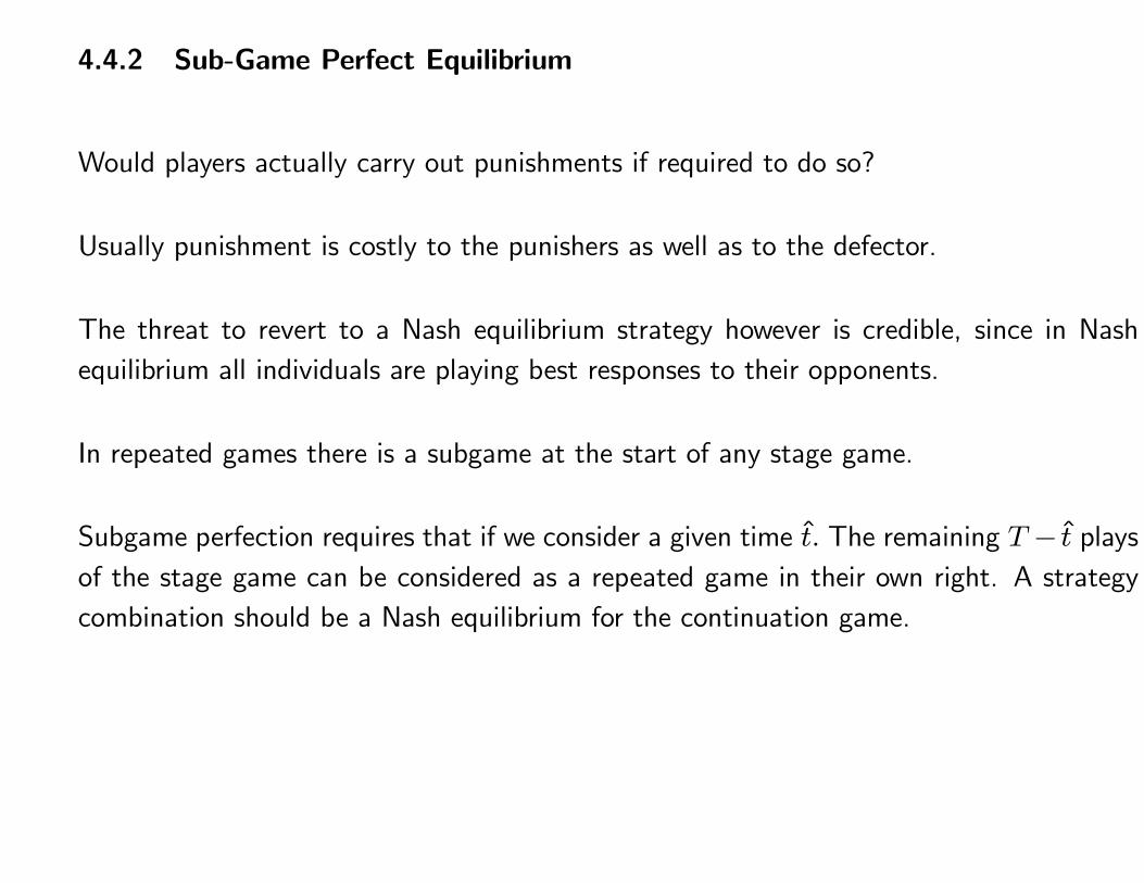
4.4.2 Sub-Game Perfect Equilibrium
Would players actually carry out punishments if required to do so?
Usually punishment is costly to the punishers as well as to the defector.
The threat to revert to a Nash equilibrium strategy however is credible, since in Nash
equilibrium all individuals are playing best responses to their opponents.
In repeated games there is a subgame at the start of any stage game.
Subgame perfection requires that if we consider a given time t. The remaining T − t plays
of the stage game can be considered as a repeated game in their own right. A strategy
combination should be a Nash equilibrium for the continuation game.
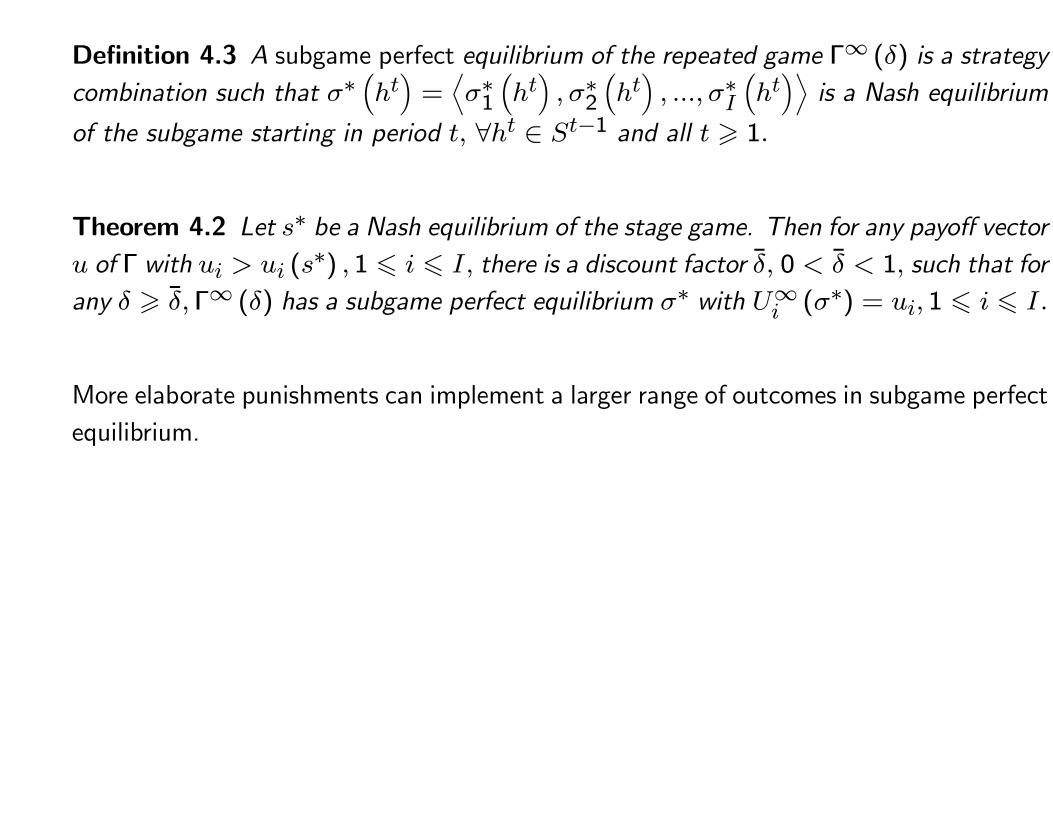
Definition 4.3 A subgame perfect equilibrium of the repeated game Γ∞ (δ) is a strategy
combination such that σ∗(ht)=⟨σ∗1
(ht), σ∗2
(ht), ..., σ∗I
(ht)⟩
is a Nash equilibrium
of the subgame starting in period t, ∀ht ∈ St−1 and all t � 1.
Theorem 4.2 Let s∗ be a Nash equilibrium of the stage game. Then for any payoff vector
u of Γ with ui > ui (s∗) , 1 � i � I, there is a discount factor δ, 0 < δ < 1, such that for
any δ � δ,Γ∞ (δ) has a subgame perfect equilibrium σ∗ with U∞i (σ∗) = ui, 1 � i � I.
More elaborate punishments can implement a larger range of outcomes in subgame perfect
equilibrium.
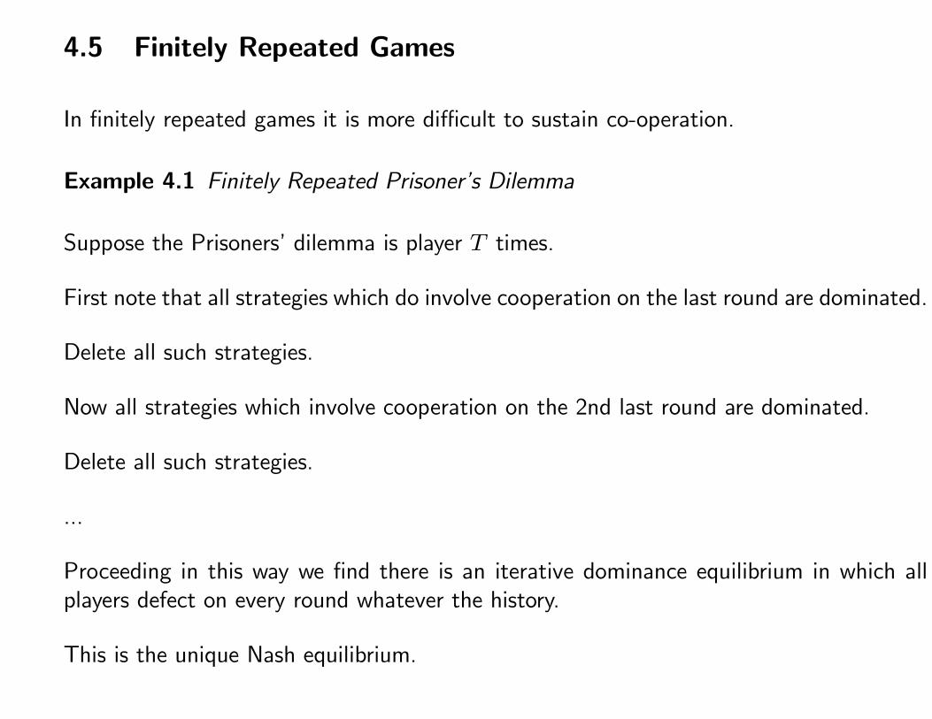
4.5 Finitely Repeated Games
In finitely repeated games it is more difficult to sustain co-operation.
Example 4.1 Finitely Repeated Prisoner’s Dilemma
Suppose the Prisoners’ dilemma is player T times.
First note that all strategies which do involve cooperation on the last round are dominated.
Delete all such strategies.
Now all strategies which involve cooperation on the 2nd last round are dominated.
Delete all such strategies.
...
Proceeding in this way we find there is an iterative dominance equilibrium in which allplayers defect on every round whatever the history.
This is the unique Nash equilibrium.
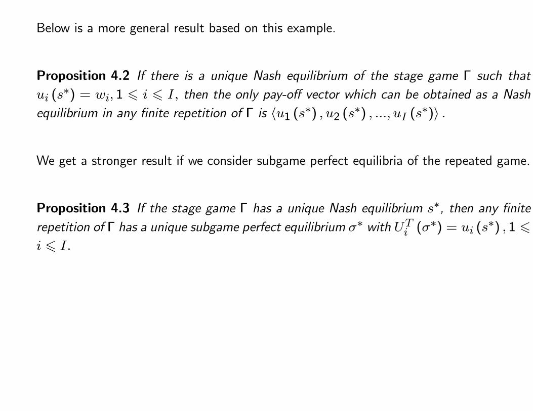
Below is a more general result based on this example.
Proposition 4.2 If there is a unique Nash equilibrium of the stage game Γ such that
ui (s∗) = wi, 1 � i � I, then the only pay-off vector which can be obtained as a Nash
equilibrium in any finite repetition of Γ is 〈u1 (s∗) , u2 (s
∗) , ..., uI (s∗)〉 .
We get a stronger result if we consider subgame perfect equilibria of the repeated game.
Proposition 4.3 If the stage game Γ has a unique Nash equilibrium s∗, then any finite
repetition of Γ has a unique subgame perfect equilibrium σ∗ with UTi (σ∗) = ui (s
∗) , 1 �
i � I.
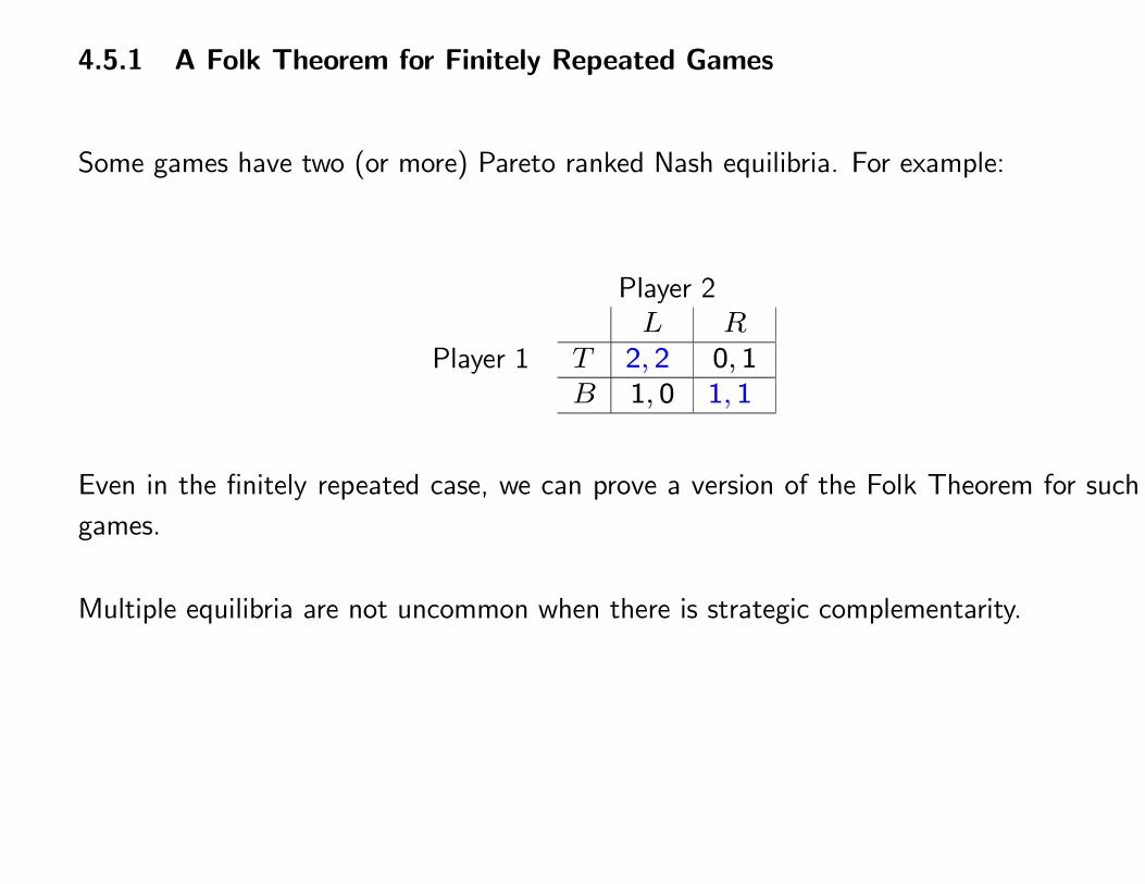
4.5.1 A Folk Theorem for Finitely Repeated Games
Some games have two (or more) Pareto ranked Nash equilibria. For example:
Player 2
Player 1L R
T 2, 2 0, 1B 1, 0 1, 1
Even in the finitely repeated case, we can prove a version of the Folk Theorem for such
games.
Multiple equilibria are not uncommon when there is strategic complementarity.
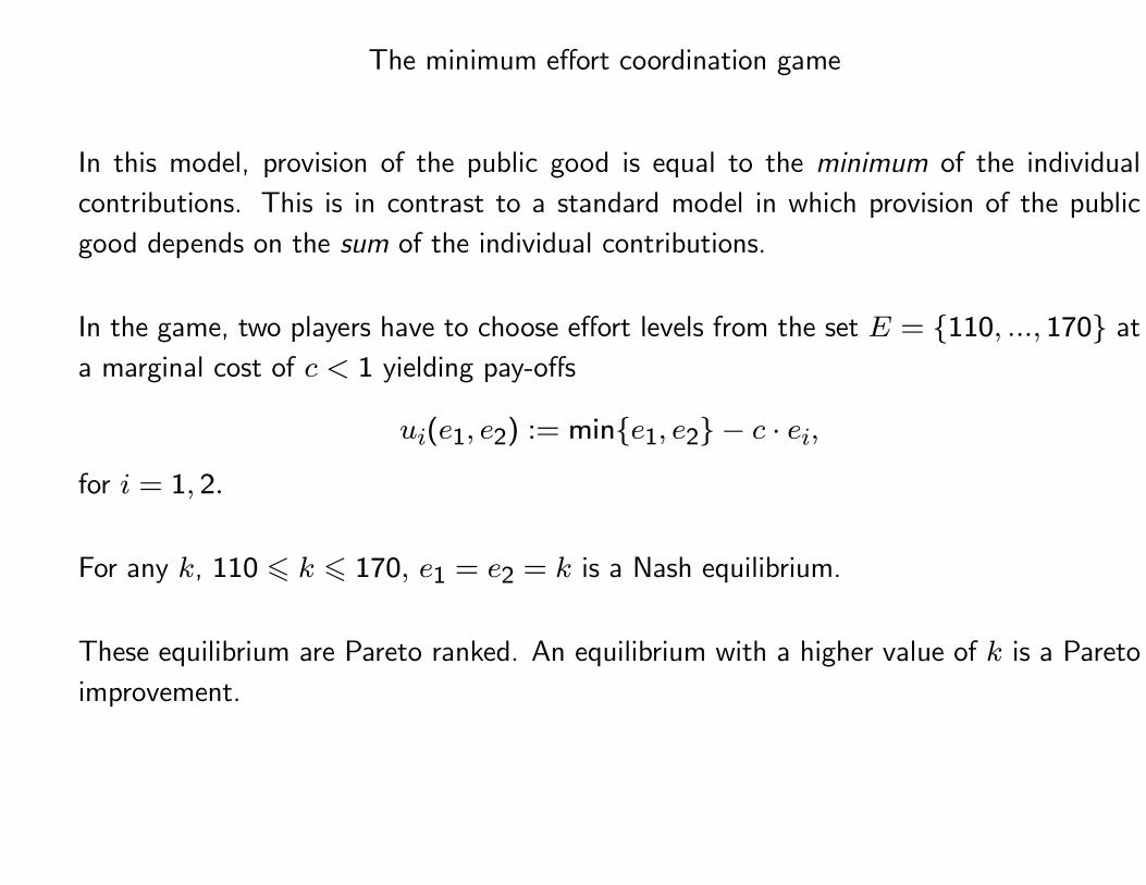
The minimum effort coordination game
In this model, provision of the public good is equal to the minimum of the individual
contributions. This is in contrast to a standard model in which provision of the public
good depends on the sum of the individual contributions.
In the game, two players have to choose effort levels from the set E = {110, ..., 170} at
a marginal cost of c < 1 yielding pay-offs
ui(e1, e2) := min{e1, e2} − c · ei,
for i = 1, 2.
For any k, 110 � k � 170, e1 = e2 = k is a Nash equilibrium.
These equilibrium are Pareto ranked. An equilibrium with a higher value of k is a Pareto
improvement.
Theorem 4.3 If a game Γ has at least two Nash equilibria s∗ and s∗∗ with ui (s∗) >
ui (s∗∗) , 1 � i � I, then there exists δ, 0 < δ < 1 and T
(t′)
such that any pay-off
vector u with ui > ui (s∗) can be implemented for the first t′ periods as a sub-game
perfect equilibrium of any finitely repeated game ΓT (δ) with T � T(t′)
and δ � δ.
Subgame perfection implies that a Nash equilibrium must be played in the last round.
However, in this case, it is possible to punish deviators by switching to the Pareto inferior
Nash equilibrium.
Cooperation can also be sustained in finitely repeated games if there is incomplete infor-
mation. See the discussion of the Prisoners’ Dilemma in Section 3.7.2.
Again the outcome is not unique since there are many irrational types an opponent can
have.
4.6 Conclusion
Concepts such as reputation and punishment can be modelled by repeated games.
This solves some paradoxes in one shot games such as lack of cooperation in the prisoners’
dilemma.
The cost is that repeated games typically have a continuum of equilibria.
Thus it is not possible to make precise predictions about play.
There is a stark difference between infinitely repeated and finitely repeated games.
Cooperation can be sustained in infinitely repeated games but not in finitely repeated
games, (in general).
This may explain why firms exist. Firms are (potentially) infinitely lived. Thus they find it
easier than individuals to build a reputation for good quality products and honest dealing.
People often cooperate even though they have finite lives.
This is compatible with the theory of repeated games.
Suppose it is randomly determined after each stage whether or not to play a further round.
If there is always a positive probability of further play then cooperation can be sustained.
However the game will end in finite time with probability 1.
Cooperation can be sustained whenever there is a possibility that the relationship will
continue.
In experiments, if the is played more than once then subjects may treat the experiment
as a repeated game and cooperate at the expense of the experimenter.
4.7 Oligopoly
To be completed
The Cournot quantities are equilibrium outcomes of a repeated Bertrand game.
The Bertrand prices are equilibrium outcomes of a repeated Cournot game.

5
6
7
8 PREDATORY PRICING
8.0.1 INTRODUCTION
REFERENCES Tirole Ch. 9, p.367-377.
Kreps, D., 1990, A Course in Microeconomic Theory, Harvester Wheatsheaf, p.468-480.
THIS TOPIC INVESTIGATES HOW A FIRM CAN OBTAIN A STRATEGIC ADVAN-
TAGE BY MANIPULATING THE BELIEFS OF RIVALS.
LIMIT PRICING AN INCUMBENT CHARGES LESS THAN THE MONOPOLY
PRICE IN ORDER TO DETER ENTRY.
PREDATORY PRICING A FIRM CHARGES A LOW PRICE TO INDUCE EXIT.
8.0.2 AMERICAN AIRLINES
AMERICAN AIRLINES IS THE DOMINANT CARRIER AT DALLAS-FORT WORTH
(DFW) AIRPORT.
1995-7 SEVERAL LOW COST CARRIERS ENTERED ON VARIOUS ROUTES FROM
DFW.
THE ENTRANTS CHARGED MARKEDLY LOWER FARES.
AMERICAN RESPONDED BY REDUCING ITS OWN FARES AND INCREASING THE
NUMBER OF FLIGHTS ON ROUTES SERVED BY THE ENTRANTS.
IN EVERY CASE THE LOW FARE CARRIER EVENTUALLY LEFT THE MARKET.
THEN AMERICAN REDUCED THE NUMBER OF FLIGHTS AND RAISED PRICES TO
PRE-ENTRY LEVELS.
PROBLEM
Why should a low pre-entry price convince an entrant to stay out?
Assume:
• It is more profitable to accommodate entry than to fight a price war.
• The incumbent practices limit pricing and sets a price so low that entry is not prof-
itable.
If the entrant ignores the low price and enters anyway, the incumbent has the choice of:
1. raising price and accommodating entry which gives a small profit,
2. keeping the same price and making losses.
In others words the threat to charge a low post entry price is not credible.
The limit pricing argument appears to assume that the post-entry price will be the same
as the pre-entry price.
However since price can be changed quickly there is no reason to assume that price will
remain lower post entry.
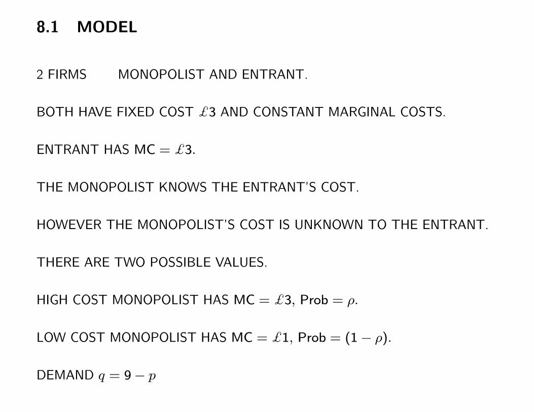
8.1 MODEL
2 FIRMS MONOPOLIST AND ENTRANT.
BOTH HAVE FIXED COST $3 AND CONSTANT MARGINAL COSTS.
ENTRANT HAS MC = $3.
THE MONOPOLIST KNOWS THE ENTRANT’S COST.
HOWEVER THE MONOPOLIST’S COST IS UNKNOWN TO THE ENTRANT.
THERE ARE TWO POSSIBLE VALUES.
HIGH COST MONOPOLIST HAS MC = $3, Prob = ρ.
LOW COST MONOPOLIST HAS MC = $1, Prob = (1− ρ).
DEMAND q = 9− p
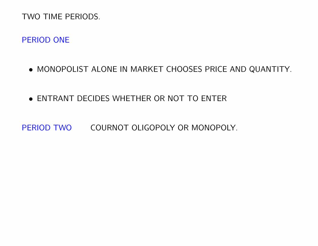
TWO TIME PERIODS.
PERIOD ONE
• MONOPOLIST ALONE IN MARKET CHOOSES PRICE AND QUANTITY.
• ENTRANT DECIDES WHETHER OR NOT TO ENTER
PERIOD TWO COURNOT OLIGOPOLY OR MONOPOLY.
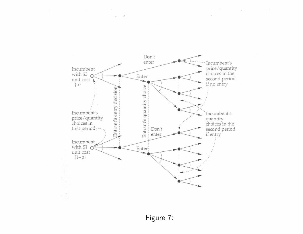
Figure 7:
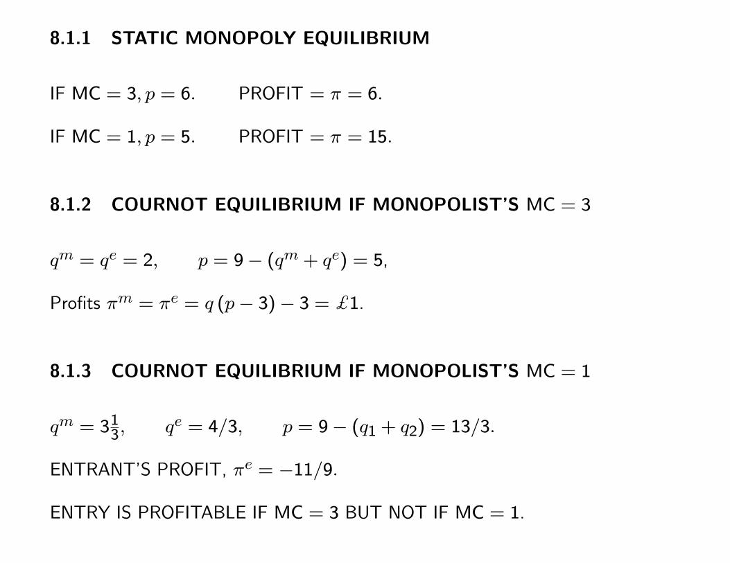
8.1.1 STATIC MONOPOLY EQUILIBRIUM
IF MC = 3, p = 6. PROFIT = π = 6.
IF MC = 1, p = 5. PROFIT = π = 15.
8.1.2 COURNOT EQUILIBRIUM IF MONOPOLIST’S MC = 3
qm = qe = 2, p = 9− (qm+ qe) = 5,
Profits πm = πe = q (p− 3)− 3 = $1.
8.1.3 COURNOT EQUILIBRIUM IF MONOPOLIST’S MC = 1
qm = 313, qe = 4/3, p = 9− (q1 + q2) = 13/3.
ENTRANT’S PROFIT, πe = −11/9.
ENTRY IS PROFITABLE IF MC = 3 BUT NOT IF MC = 1.
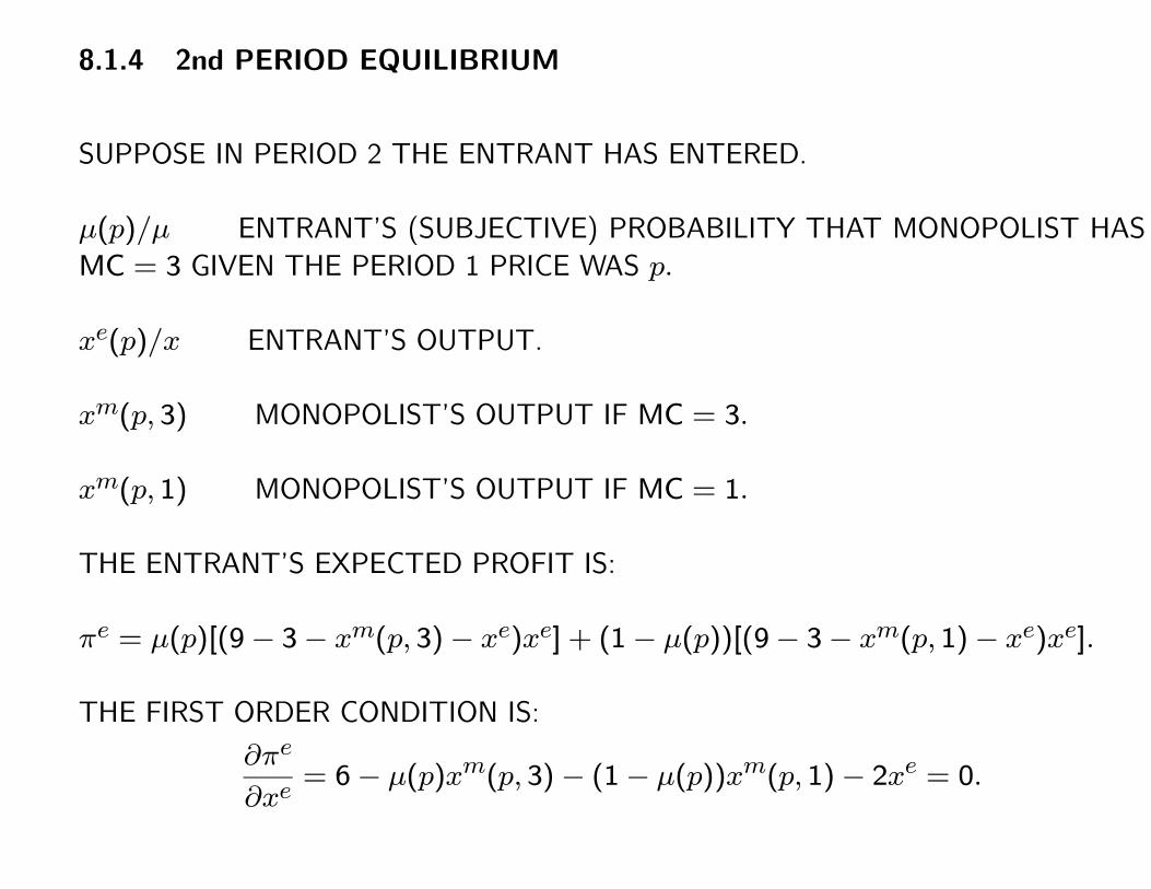
8.1.4 2nd PERIOD EQUILIBRIUM
SUPPOSE IN PERIOD 2 THE ENTRANT HAS ENTERED.
µ(p)/µ ENTRANT’S (SUBJECTIVE) PROBABILITY THAT MONOPOLIST HAS
MC = 3 GIVEN THE PERIOD 1 PRICE WAS p.
xe(p)/x ENTRANT’S OUTPUT.
xm(p, 3) MONOPOLIST’S OUTPUT IF MC = 3.
xm(p, 1) MONOPOLIST’S OUTPUT IF MC = 1.
THE ENTRANT’S EXPECTED PROFIT IS:
πe = µ(p)[(9− 3− xm(p, 3)− xe)xe] + (1− µ(p))[(9− 3− xm(p, 1)− xe)xe].
THE FIRST ORDER CONDITION IS:
∂πe
∂xe= 6− µ(p)xm(p, 3)− (1− µ(p))xm(p, 1)− 2xe = 0.
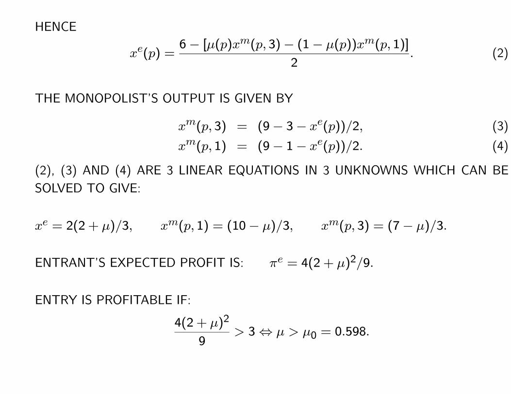
HENCE
xe(p) =6− [µ(p)xm(p, 3)− (1− µ(p))xm(p, 1)]
2. (2)
THE MONOPOLIST’S OUTPUT IS GIVEN BY
xm(p, 3) = (9− 3− xe(p))/2, (3)
xm(p, 1) = (9− 1− xe(p))/2. (4)
(2), (3) AND (4) ARE 3 LINEAR EQUATIONS IN 3 UNKNOWNS WHICH CAN BE
SOLVED TO GIVE:
xe = 2(2 + µ)/3, xm(p, 1) = (10− µ)/3, xm(p, 3) = (7− µ)/3.
ENTRANT’S EXPECTED PROFIT IS: πe = 4(2 + µ)2/9.
ENTRY IS PROFITABLE IF:
4(2 + µ)2
9> 3⇔ µ > µ0 = 0.598.
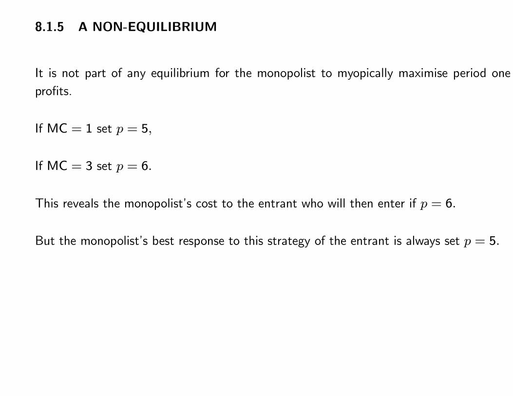
8.1.5 A NON-EQUILIBRIUM
It is not part of any equilibrium for the monopolist to myopically maximise period one
profits.
If MC = 1 set p = 5,
If MC = 3 set p = 6.
This reveals the monopolist’s cost to the entrant who will then enter if p = 6.
But the monopolist’s best response to this strategy of the entrant is always set p = 5.
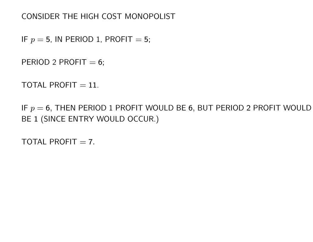
CONSIDER THE HIGH COST MONOPOLIST
IF p = 5, IN PERIOD 1, PROFIT = 5;
PERIOD 2 PROFIT = 6;
TOTAL PROFIT = 11.
IF p = 6, THEN PERIOD 1 PROFIT WOULD BE 6, BUT PERIOD 2 PROFIT WOULD
BE 1 (SINCE ENTRY WOULD OCCUR.)
TOTAL PROFIT = 7.
Thus the incumbent will not always set the standard monopoly price in the first period.
There are two possible types of equilibrium.
• A pooling equilibrium where the high and low cost monopolist set the same price.
• A screening equilibrium where the high cost monopolist sets a higher price than the
low cost monopolist.
8.1.6 POOLING EQUILIBRIUM
MONOPOLIST: BOTH TYPES OF MONOPOLIST SET p = $5 IN THE FIRST
PERIOD.
IN THE SECOND PERIOD
• THEY SET THE MONOPOLY PRICE IF NO ENTRY,
• PRODUCE THE COURNOT OUTPUT IF THERE IS ENTRY.
ENTRANT: ENTERS IF AND ONLY IF p > $5. PRODUCES THE COURNOT
OUTPUT IF (S)HE ENTERS.
ENTRANT’S BELIEF IS µ(5) = ρ, µ(p) = 1, IF p > 5.
ρ = PRIOR PROBABILITY {MC = 3}.
THESE ARE EQUILIBRIUM STRATEGIES PROVIDED ρ < 0.598.
THE ENTRANT RECEIVES NO INFORMATION FROM SEEING THE FIRST PERIOD
PRICE. HENCE, (S)HE DOES NOT REVISE HIS/HER BELIEFS:
µ(p) = ρ < 0.598.
BUTWE HAVE ALREADY FOUND THAT ENTRY IS NOT PROFITABLE IF µ < 0.598.
FOR THE HIGH COST MONOPOLIST IT IS WORTH SACRIFICING THE FIRST PE-
RIOD PROFITS TO RETAIN MONOPOLY POWER IN THE SECOND PERIOD.
8.1.7 WELFARE IMPLICATIONS (POOLING)
THERE IS LESS ENTRY THAN UNDER SYMMETRIC INFORMATION.
THE HIGH COST MONOPOLIST CHARGES A LOWER PRICE IN THE FIRST PERIOD
AND A HIGHER PRICE IN THE SECOND PERIOD COMPARED TO SYMMETRIC
INFORMATION.
THE LOW COST MONOPOLIST CHARGES THE SAME PRICE IN THE FIRST AND
SECOND PERIODS.
LIMIT PRICING DOES OCCUR.
NO CLEAR WELFARE IMPLICATIONS CAN BE DRAWN. FIRST PERIOD PRICES ARE
LOWER BUT SECOND PERIOD PRICES ARE HIGHER THAN WITH SYMMETRIC
INFORMATION.
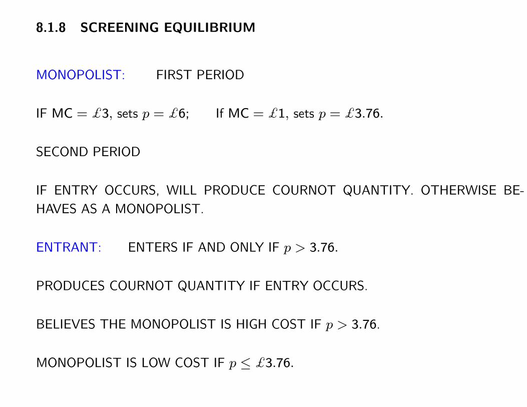
8.1.8 SCREENING EQUILIBRIUM
MONOPOLIST: FIRST PERIOD
IF MC = $3, sets p = $6; If MC = $1, sets p = $3.76.
SECOND PERIOD
IF ENTRY OCCURS, WILL PRODUCE COURNOT QUANTITY. OTHERWISE BE-
HAVES AS A MONOPOLIST.
ENTRANT: ENTERS IF AND ONLY IF p > 3.76.
PRODUCES COURNOT QUANTITY IF ENTRY OCCURS.
BELIEVES THE MONOPOLIST IS HIGH COST IF p > 3.76.
MONOPOLIST IS LOW COST IF p ≤ $3.76.
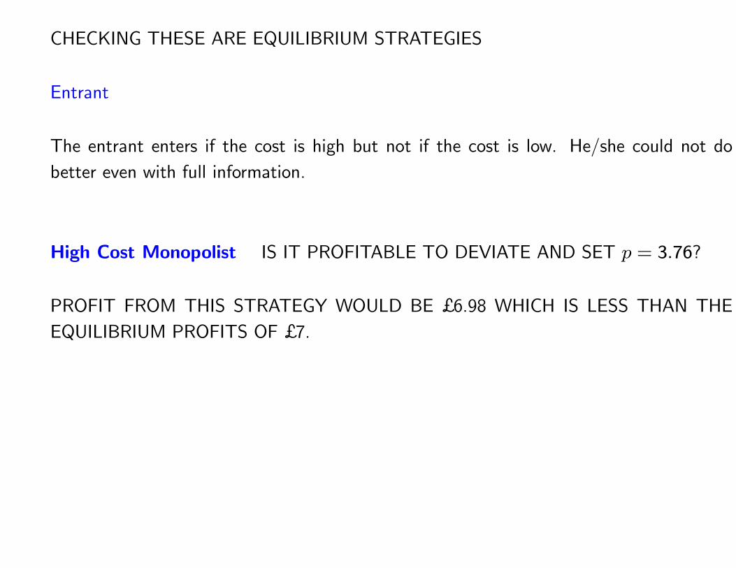
CHECKING THESE ARE EQUILIBRIUM STRATEGIES
Entrant
The entrant enters if the cost is high but not if the cost is low. He/she could not do
better even with full information.
High Cost Monopolist IS IT PROFITABLE TO DEVIATE AND SET p = 3.76?
PROFIT FROM THIS STRATEGY WOULD BE £6.98 WHICH IS LESS THAN THE
EQUILIBRIUM PROFITS OF £7.
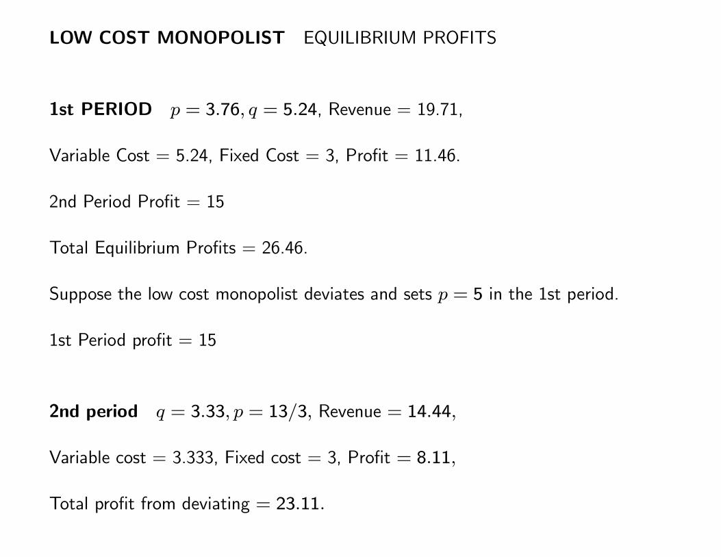
LOW COST MONOPOLIST EQUILIBRIUM PROFITS
1st PERIOD p = 3.76, q = 5.24, Revenue = 19.71,
Variable Cost = 5.24, Fixed Cost = 3, Profit = 11.46.
2nd Period Profit = 15
Total Equilibrium Profits = 26.46.
Suppose the low cost monopolist deviates and sets p = 5 in the 1st period.
1st Period profit = 15
2nd period q = 3.33, p = 13/3, Revenue = 14.44,
Variable cost = 3.333, Fixed cost = 3, Profit = 8.11,
Total profit from deviating = 23.11.
AMERICAN AIRLINES
It would be difficult for a small entrant to determine the cost for American Airlines.
The marginal cost of a passenger from Wichita to Dallas depends on the cost of the plane
crew etc.
minus the profit made on any onward flight e.g. Dallas-Los Angeles.
The upline/downline contributions would be difficult for an outsider to determine.
Thus an entrant might perceive significant uncertainty concerning American Airlines costs.
8.1.9 WELFARE EFFECTS (SCREENING EQUILIBRIUM)
LIMIT PRICING DOES OCCUR.
ENTRY OCCURS EXACTLY WHEN IT WOULD HAVE DONE UNDER SYMMETRIC
INFORMATION.
COMPARED TO SYMMETRIC INFORMATION:
• THE LOW COST MONOPOLIST CHARGES A LOWER PRICE IN THE FIRST
PERIOD;
• THE HIGH COST MONOPOLIST CHARGES THE SAME PRICE.
THUS THERE IS A GAIN IN TOTAL SURPLUS COMPARED TO SYMMETRIC INFOR-
MATION.

ANTI- TRUST
AREEDA-TURNER STANDARD ‘PRICES ARE PREDATORY IF THEY ARE BE-
LOW SHORT RUN MARGINAL COST.’
NOTE IN BOTH THE POOLING AND THE SCREENING EQUILIBRIA THE LIMIT
PRICES ARE ABOVE MARGINAL COST.
8.2 EXTENSIONS
8.2.1 EXIT
IF FIRM 2 IS ALREADY IN THE INDUSTRY, BUT IS UNCERTAIN OF FIRM 1’S COSTS
THEN LIMIT PRICING MAY BE USED TO INDUCE FIRM 2 TO EXIT.
SUCH A STRATEGY IS USUALLY REFERRED TO AS PREDATORY PRICING

8.2.2 PREDATION FOR MERGER
Assume that Firm 2 is already in the industry.
• Firm 1 may wish to buy Firm 2.
• Predatory pricing may be used to achieve a merger on more favourable terms.
Magee Journal of Law and Economics (1958) Why prey? Why not just merge? Industry
profits are reduced in the predation period.
• May violate antitrust law;
• Merger on favourable terms may encourage future entry.
AMERICAN TOBACCO
Acquired 43 competitors in the period 1891-1906.
Prior to the acquisition American Tobacco engaged in predatory pricing in the targets
market.
They used “fighting brands”. These are low cost brands only available in the prey’s
territory.
This was estimated to lower the cost of acquisition by 60%.
Even firms which were not preyed upon sold out cheaply.
• This supports the view that predatory pricing sends a signal about future market
conditions.
8.3 CONCLUSION
LIMIT PRICING DOES NOT MAKE SENSE WITHOUT UNCERTAINTY.
LIMIT PRICING MAY BE EXPLAINED AS THE INCUMBENT SIGNALLING TO THE
ENTRANT THAT HIS/HER COSTS ARE LOW.
WHILE LIMIT PRICING MAY OCCUR, IT IS NOT NECESSARILY HARMFUL.
THE SCREENING EQUILIBRIUM IS WELFARE IMPROVING AND THE POOLING
EQUILIBRIUM HAS AMBIGUOUS EFFECTS ON WELFARE.
SIMILAR RESULTS COULD BE OBTAINED IF:
• THERE WAS UNCERTAINTY ABOUT THE LEVEL OF DEMAND.
• IT WAS UNCERTAINWHETHER THE INCUMBENT AIMED TOMAXIMISE PROFI
OR MAXIMISE MARKET SHARE.
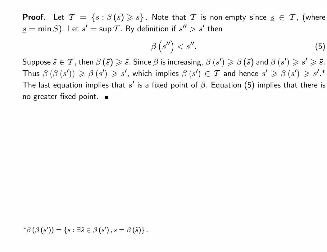
Proof. Let T = {s : β (s) � s} . Note that T is non-empty since s ∈ T , (where
s = minS). Let s′ = supT . By definition if s′′ > s′ then
β(s′′)< s′′. (5)
Suppose s ∈ T , then β (s) � s. Since β is increasing, β(s′)� β (s) and β
(s′)� s′ � s.
Thus β(β(s′))� β
(s′)� s′, which implies β
(s′)∈ T and hence s′ � β
(s′)� s′.∗
The last equation implies that s′ is a fixed point of β. Equation (5) implies that there is
no greater fixed point.
∗β (β (s′)) = {s : ∃s ∈ β (s′) , s = β (s)} .