Essays in Industrial Organisation

Seyed Farshad FATEMI ARDESTANI

A thesis submitted for

PhD in Economics

University College London

25 May 2009

2

I, Seyed Farshad FATEMI ARDESTANI, confirm that the work presented in this thesis

is my own. Where information has been derived from other sources, I confirm that this

has been indicated in the thesis.

3

Abstract

This thesis consists of three independent chapters:

In the first chapter, we consider a Hotelling model of price competition where firms

may acquire information regarding the preferences (i.e. “location”) of customers. By

purchasing additional information, a firm has a finer partition regarding customer

preferences, and its pricing decisions must be measurable with respect to this partition.

If information acquisition decisions are common knowledge at the point where firms

compete via prices, we show that a pure strategy subgame perfect equilibrium exists,

and that there is “excess information acquisition” from the point of view of the firms. If

information acquisition decisions are private information, a pure strategy equilibrium

fails to exist. We compute a mixed strategy equilibrium for a range of parameter values.

The second chapter investigates a case of national versus regional pricing.

Competition authorities frequently view price discrimination by firms as detrimental to

consumers. In the case of the UK supermarket industry they suggested a move to

uniform pricing. Yet theoretical predictions are ambiguous about whether third degree

price discrimination is beneficial or detrimental to consumers, and in general there will

be some consumers who benefit while other lose out. In this chapter, we estimate the

impact that the move from regional to uniform pricing had on Tesco’s profits and

consumer's surplus. We estimate an AIDS model of consumer expenditure in the eggs

market in a multi-stage budgeting framework allowing for very flexible substitution

patterns between products at the bottom level. We use data on farm gate prices to

instrument price in the demand equation. Our results suggest that switching to a

regional pricing policy can potentially increase Tesco’s profit on eggs by 37%.

However, while there are winners and losers, the overall effect on consumer welfare is

not significant.

4

In the third chapter, we study the kidney market in Iran. The most effective

treatment for end-stage renal disease is a kidney transplant. While the supply of

cadaveric kidneys is limited, the debate has been focused on the effects of the existence

of a free market for human organs. Economists as well as medical and legal researchers

are divided over the issue. Iran has a unique kidney market which has been in place for

over 20 years, frequently reporting surprising success in reducing the waiting list for

kidneys. This paper demonstrates how the Iranian system works and estimates the

welfare effect of this system.

5

To my parents;

for their inspirational role in my life

&

To my family;

for their support during this course.

6

Acknowledgment

Completion of this thesis would not have been possible without the support of many

people. The author wishes to express her gratitude to his principal supervisor, Prof. V.

Bhaskar, who was abundantly helpful and offered invaluable support and guidance. The

initial idea of the first chapter was from him. Deepest gratitude is also due to second

supervisor, Prof. Rachel Griffith, who provided access to the data set for the second

chapter as well as insightful comments and guidance. The author also wishes to thank

other faculty members as well as research students at the department of economics,

University College London.

The author would also like to convey thanks to Kidney Foundation especially Mr.

Ghasemi and Mrs. Shaban-Kareh for providing access to foundation data base. Dr.

Alireza Heidary from the Organ Procurement Centre at the Iranian Ministry of Health

also was very helpful in order to improve author’s understanding of the Iranian kidney

donation system.

The author also wishes to thank Iranian Ministry of Science, Research, and

Technology, and Sharif University of Technology for the PhD scholarship. Thanks are

also due to the ESRC Centre for Economic Learning and Social Evolution at University

College London for the financial support.

The author wishes to express her love and gratitude to her beloved family; for their

understanding and endless love, during his studies.

7

Table of Contents

LIST OF TABLES ..................................................................................................................................................... 9

LIST OF FIGURES .................................................................................................................................................11

CHAPTER 1 INFORMATION ACQUISITION AND PRICE DISCRIMINATION.....................13

1.1. INTRODUCTION......................................................................................................................... 13

1.2. THE MODEL ............................................................................................................................... 16 1.3. THE TWO-STAGE GAME......................................................................................................... 21

1.3.1. Scenario One: Neither firm acquires information ..................................................................21 1.3.2. Scenario Two: Both firms acquire information.......................................................................22

1.3.3. Scenario Three: Only firm A acquires information................................................................31 1.3.4. Outcome of the Two-Stage Game ................................................................................................33

1.4. THE SIMULTANEOUS MOVE GAME ...................................................................................... 35 1.4.1. Case 1: None of the firms acquire information........................................................................35

1.4.2. Case 2: Both firms acquire information ....................................................................................35 1.4.3. Case 3: Only firm A acquires information................................................................................37

1.4.4. Outcome of the Simultaneous Move Game ...............................................................................39

1.5. COMPARING THE TWO-STAGE GAME WITH THE MULTI -STORE EXAMPLE............... 39 1.5.1. First sub-game; None of the firms opens a new store ............................................................41 1.5.2. Second sub-game; Both firms open a new store ......................................................................41

1.5.3. Third sub-game; Only firm A opens a new store .....................................................................43

1.5.4. Outcome of the multi-store game ................................................................................................44

1.6. SUMMARY AND CONCLUSION................................................................................................ 46

APPENDIX 1.A............................................................................................................................................ 47 APPENDIX 1.B ............................................................................................................................................ 56

APPENDIX 1.C............................................................................................................................................ 61

8

CHAPTER 2 NATIONAL PRICING VERSUS REGIONAL PRICING; AN INVESTIGATION

INTO THE UK EGG MARKET ................................................................................................67

2.1. INTRODUCTION......................................................................................................................... 67

2.2. THEORETICAL MODEL............................................................................................................ 69 2.2.1. Firm pricing .....................................................................................................................................69 2.2.2. Consumer behaviour ......................................................................................................................71

2.2.3. Price Elasticities..............................................................................................................................78

2.3. DATA ........................................................................................................................................... 80 2.3.1. Characteristics.................................................................................................................................80 2.3.2. Descriptive Analysis .......................................................................................................................82

2.4. RESULTS ..................................................................................................................................... 86 2.4.1. Demand System Estimates ............................................................................................................86

2.4.2. Marginal Costs ................................................................................................................................91 2.4.3. Profit maximising prices ...............................................................................................................93

2.4.4. Impact on Retailer Profits.............................................................................................................95 2.4.5. Impact on Consumer Welfare ......................................................................................................95

2.5. SUMMARY AND CONCLUSION................................................................................................ 97 APPENDIX 2.A............................................................................................................................................ 98

APPENDIX 2.B ..........................................................................................................................................100

CHAPTER 3 THE MARKET FOR KIDNEYS IN IRAN ....................................................................111

3.1. INTRODUCTION.......................................................................................................................111

3.2. LITERATURE REVIEW............................................................................................................118 3.2.1. Kidney Market ...............................................................................................................................118

3.2.2. Kidney Exchange Mechanisms ..................................................................................................120

3.3. IRAN’S CASE............................................................................................................................121 3.3.1. Background ....................................................................................................................................121 3.3.2. Institutions......................................................................................................................................121

3.3.3. How Does Unrelated Kidney Donation in Iran Work? ........................................................122

3.4. DATA .........................................................................................................................................127

3.5. MODEL ......................................................................................................................................133 3.6. SUMMARY AND CONCLUSION..............................................................................................136

REFERENCES .....................................................................................................................................................140

9

List of Tables

Table 1.1 Firm A’s chain of decision statements...................................................................................... 27

Table 1.2 Firm A’s chain of decision statements with a constant information cost ....................... 58

Table 1.3 Firm A’s chain of decision statements with a general information cost function ........ 61

Table 2.1 Distribution of eggs purchased in Tesco, Dec 2001 – Dec 2004 ........................................ 82

Table 2.2 Categories of eggs .......................................................................................................................... 83

Table 2.3 The summary of Tesco regional egg sales ............................................................................... 84

Table 2.4 London: bottom level results for Caged and Barn using two different price

indexes ............................................................................................................................................... 86

Table 2.5 London: bottom level results for Free range .......................................................................... 87

Table 2.6 Conditional own price elasticities for bottom level, by region........................................... 88

Table 2.7 London: middle level results ....................................................................................................... 89

Table 2.8 Income and price elasticities for the top level ........................................................................ 90

Table 2.9 Unconditional own price elasticities.......................................................................................... 91

Table 2.10 Estimated marginal costs and farm gate prices..................................................................... 92

Table 2.11 The average national and regional profit maximising prices for all categories............ 94

Table 2.12 Summary statistics for the change in consumer welfare as a result of switching

to a regional pricing policy......................................................................................................... 97

Table 2.B1 Summary statistics....................................................................................................................... 100

Table 2.B2 Bottom level results for Caged and Barn, coefficients for Small / Medium

/Mixed (Value) and conditional own-price elasticities using approximate price

index................................................................................................................................................. 105

10

Table 2.B3 Bottom level results for Caged and Barn, coefficients for Small / Medium

/Mixed (Value) using exact price index.................................................................................. 106

Table 2.B4 Bottom level results for Free Range, coefficients for the three sub-categories

and conditional own-price elasticities using approximate price index.......................... 107

Table 2.B5 Bottom level results for Free Range, coefficients for the three sub-categories

using exact price index................................................................................................................ 109

Table 2.B6 Middle level results for all ten regions ................................................................................... 110

Table 3.1 Survival probability for different treatments...................................................................... 113

Table 3.2 The number of live and cadaveric kidney transplantation 1985 – 2006 ....................... 115

Table 3.3 The compatibility rule for blood and organ donation........................................................ 117

Table 3.4 The ABO and RhD blood types distribution of recipients ................................................ 128

Table 3.5 The ABO blood type distribution of recipients .................................................................... 128

Table 3.6 The sex of recipients of each type of kidney......................................................................... 129

Table 3.7 The sex of donors of each type of kidney............................................................................... 129

Table 3.8 Age distribution of recipients and donors ............................................................................. 130

Table 3.9 Joint ABO and RdH frequency of transplants for recipients and donors.................... 131

Table 3.10 Average waiting time for recipients based on the blood type of both parties ............. 132

Table 3.A1 Number of kidney transplants per million population for some countries in

2006 ................................................................................................................................................. 137

Table 3.A2 The ABO and RdH blood type distribution of Iran provinces ........................................ 138

Table 3.A3 ABO allele frequencies in 21 Iranian population groups .................................................. 139

11

List of Figures

Figure 1.1 The decision tree for each firm regarding the information acquisition ......................... 19

Figure 1.2 A price function consistent with the information acquisition definition......................... 20

Figure 1.3 Three possible segmentation scenarios .................................................................................... 21

Figure 1.4 Four different scenarios for the two-stage game ................................................................... 21

Figure 1.5 An example of the equilibrium strategy for firm A in the second scenario ................... 30

Figure 1.6 The preferred number of segments and the profit of each firm as a function of

the ratio of information cost over transportation cost......................................................... 30

Figure 1.7 The length of shared and loyal segments as a function of the ratio of

information cost over transportation cost............................................................................... 31

Figure 1.8 An example of the equilibrium strategy for the firms in the third scenario.................. 33

Figure 1.9 The outcome of the game when 00 →τ ................................................................................ 33

Figure 1.10 Firm A’s profit for four different scenarios versus the

information/transportation cost ratio....................................................................................... 34

Figure 1.11 The multi-store retailer game .................................................................................................... 41

Figure 1.12 The 2nd sub-game of the multi-store retailer game .............................................................. 41

Figure 1.13 The 3rd sub-game of the multi-store retailer game .............................................................. 43

Figure 1.14 The payoffs in the multi-store retailer game ......................................................................... 45

Figure 1.15 The probability of choosing the non-information acquisition strategy in the

mixed strategy equilibrium......................................................................................................... 66

Figure 1.16 The prices and profit in the mixed strategy equilibrium.................................................... 66

Figure 2.1 The three-level budgeting model................................................................................................ 72

Figure 2.2 Trend of egg categories’ expenditure shares over time in the London region.............. 78

Figure 2.3 Average price of caged eggs at Tesco........................................................................................ 81

12

Figure 2.4 The average national and regional profit maximising prices for caged and barn

small/medium eggs ........................................................................................................................ 94

Figure 2.5 The estimated profit gain for Tesco under regional pricing policy.................................. 95

Figure 2.6 The average and range of estimated consumer gain/loss across the regions ................. 97

Figure 3.1 Demand and supply in X type markets in presence of a negative shock to

demand for X ............................................................................................................................... 135

Figure 3.2 Demand and supply in two blood-type markets in presence of a positive shock

to demand for X............................................................................................................................ 136

13

Chapter 1

Information Acquisition and Price Discrimination

1.1. Introduction

Usually, any type of price discrimination requires customer-specific information1.

In general, it is costly to acquire information regarding customers. Recent developments

in information technology allow firms to acquire more information on their customers,

which may be used to practise price discrimination. Loyalty cards issued by

supermarkets and customer data collected by specialist companies are just two examples

of information acquisition.

Consider a model of competition between firms who are able to charge different

prices if they can distinguish customer characteristics. Most research on discriminatory

pricing assumes that the information regarding consumers is exogenously given. The

price discrimination literature concentrates on monopolistic price discrimination (Pigou,

1920; Robinson, 1933; Schmalensee, 1981; Varian, 1985; Varian, 1989; and Hamilton

& Slutsky, 2004). Such discrimination always leads to higher profits for the monopolist,

since she solves her profit maximisation problem with fewer constraints.

Some of the more recent work on competitive price discrimination concentrates on

efficiency from society’s point of view, the firm’s profit, and the number of the firms in 1 The exceptions for this claim are the case in which the firm practices price discrimination through

setting a uniform price when the cost of supply is different and when firm uses a non-linear pricing

strategy.

14

a free entry and exit case2 (Borenstein, 1985; Corts, 1998; Armstrong & Vickers, 2001;

and Bhaskar & To, 2004), but still the information regarding consumers is exogenously

given.

Bhaskar & To (2004) prove that without free entry, perfect price discrimination is

socially optimal, but in free entry case, the number of firms is always excessive.

Liu & Serfes (2004, 2005) study the relation between of the exogenously given

quality of firm information and market outcomes in oligopoly. They show that when the

information quality is low, unilateral commitments not to price discriminate arise in

equilibrium. However, once information quality is sufficiently high, firms discriminate.

Equilibrium profits are lower, the game effectively becoming a prisoners’ dilemma.

Shaffer & Zhang (2002) investigate one-to-one promotions. They assume that

customers can be contacted individually, and firms know something about each

customer’s preferences. They find that one-to-one promotions always lead to an

increase in price competition and average prices will decrease. However, they show that

if one of the firms has a cost advantage or higher quality product, the increase in its

market share may outweigh the effect of lower prices..

Corts (1998) investigates price discrimination by imperfectly competitive firms. He

shows that the intensified competition, leading to lower prices, may make firms worse

off and as a result firms may wish to avoid the discriminatory outcome. Unilateral

commitments not to price discriminate may raise firm profits by softening price

competition.

In this paper, we endogenise the information firms have by introducing an

information acquisition technology. We assume that firms decide on how many units of

information to acquire. Then each firm can charge different prices for different

customers based on the information she acquired. We study a Hotelling type model

where two firms are located at the ends of the unit interva l. Each unit of information

gives a firm a finer partition over the set of customers. Specifically, a firm’s information

consists of a partition of the unit interval, and an extra unit of information allows the

firm to split one of the subintervals into two equal-sized segments. In our benchmark

2 For a more detailed survey on recent literature in price discrimination see Armstrong (2006).

15

model, the information acquisition decisions of firms are common knowledge at the

point where firms compete via prices.

Our main result is that the equilibrium outcome is partial information acquisition,

even if information costs are arbitrarily small. Quite naturally, a firm has no incentive to

acquire information on customers who are firmly in its rival’s turf, i.e. those that it will

never serve in equilibrium. But more interestingly, we find that a firm has an incentive

not to fully acquire information on customers it competes for with the other firm. This

allows it to commit to higher prices, and thereby softens price competition. Finally, as

in the existing literature, we find that the re is “excess information acquisition” from the

point of view of the firms, in the sense that profits are lower as compared to the no

information case.

Information acquisition results in tougher competition, and lower prices. After

information acquisition stage when firms compete via prices, if two firms share the

market over a given set of customers, a decrease in the price of one firm over this

interval decreases the marginal revenue of the other firm by decreasing its market share

on this interval. As a result this reinforces the other firm to decrease its price over that

interval. We can interpret this result in context of strategic complementarity as defined

by Bulow et al (1985). In our benchmark model, pricing decisions are strategic

complements. Since a firm’s optimal price is an increasing function of her opponent’s

price. The literature on strategic complementarity finds similar results to our results

when firms’ actions are strategically complements. Fudenberg & Tirole (1984) show

that in a two stage entry game of investment, the incumbent might decide to underinvest

in order to deter entry. d’Aspremont et al (1979) consider a Hotelling framework, with

quadratic transportation costs, when firms should choose their location. They show that

in the equilibrium in order to avoid tougher competition, firms locate themselves at the

two extremes (maximum differentiation). Similarly, in our model, a firm acquires less

information in order to commit to pricing high, thereby increases the price of her rival.

We also analyse a game where a firm does not know its rival’s information

acquisition decision at the point that they compete in prices. We show, quite generally

that there is no pure strategy equilibrium in this game. We compute a mixed strategy

equilibrium for a specific example.

Section 1.2 presents the basic model. Section 1.3 analyzes the extensive form game;

where each firm observes her rival’s information partition so that the information

16

acquisition decisions are common knowledge. Section 1.4 studies the game where

information acquisition decisions are private. Section 1.5 compares our benchmark

model with a multi-store retailers’ example. Section 1.6 summarises and concludes. The

appendices 1.A and 1.B contain all the proofs.

1.2. The Model

The model is based on a simple linear city (Hotelling model) where two firms (A

and B) compete to sell their product to customers located between them. Both firms

have identical marginal costs, normalised to zero. The distance between two firms is

normalized to one; firm A is located at 0 and firm B at 1. The customers are uniformly

distributed on the interval [0,1] and the total mass of them is normalized to one. Each

customer, depending on her location and the prices charged by firms, decides to buy one

unit from any of the firms or does not buy at all. The utility of buying for each customer

has a linear representation TCPVU −−= where P stands for price, and TC represents

the transportation cost to buy from each firm that is a linear function of distance and t is

the transport cost per unit distance. Assume that V is sufficiently high to guarantee that

all the market will be served. Then the utility of the customer who is located at [ ]1,0∈x

is

( ) ( )( ) ( )

−−−−−

=BfrombuyssheifxtxPVAfrombuyssheiftxxPV

xUB

A

1. (1.1)

A unit of information enables the firm to split an interval segment of her already

recognised customers to two equal-sized sub-segments. The information about the

customers, below and above the mid-point of [0,1] interval, is revealed to the firm if it

pays a cost )0(τ . Every unit of more information enables the firm to split an already

recognised interval, [a , b] to two equal-sized sub-intervals. The cost to the firm is )(kτ

where k

ab

=−

21 (where 0Uℵ∈k ). The information cost function can be

represented by the infinite sequence ∞

0)(kτ . It seems reasonable to assume that )(kτ

is decreasing in k. Intuitively the smaller the interval, the fewer consumers on whom

information is needed. Then a reasonable assumption for the information cost function

is that τ is a decreasing function.

17

We assume a decreasing information cost function when the cost of acquiring

information on an interval [a,b] is:

kk2

)( 0ττ = , where

k

ab

=−

21 , (1.2)

and 0τ is a constant. Note that because of our information acquisition technology k is

always an integer.

By buying every extra unit of information, a firm is acquiring more specific

information with less information content in terms of the mass of customers.

The general results of the paper, i.e. the excessive information acquisition, the

trade-off between information acquisition and tougher competition, and the

characteristics of equilibrium are consistent for a wide range of information cost

functions. In appendix 1.B, we extend our results to two other functional formats.

We analyse two alternative extensive form games. In the first game, each firm

observes its rival’s information acquisition decision. That is, the information partitions

become common knowledge before firms choose prices.

The first game is defined as follows:

• Stage 1: Information acquisition: Each firm (f∈A,B) chooses a partition If of

[0,1] from a set of possible information partitions Ω

• Observation: Each firm observes the partition choice made by the other firm, e.g.

firm A observes IB. Note that firm f’s information partition remain If .

• Stage 2: Price decision: Each firm chooses [ ] 01,0: U+ℜ→fP which is

measurable with respect to If . Once prices have been chosen, customers decide

whether to buy from firm A or firm B or not to buy at all.

The vector of prices chosen by each firm in stage 2 is segment specific. In fact a

firm’s ability to price discriminate depends on the information partition that she

acquires in stage 1. Acquiring information enables the firm to set different prices for

different segments of partition.

In the second game firms do not observe their rival’s information partition. It means

that the firms simultaneously choose a partition and a vector of prices measurable with

18

their chosen partition. In order to make it simpler, the two games are called the two-

stage game and the simultaneous move game respectively.

Following we formally define the information acquisition technology. Intuitively, in

this setting when a firm decides to acquire some information about customers, it is done

by assuming binary characteristics for customers. Revealing any characteristics divides

known segments customers to two sub-segments. We assume that these two sub-

segments have equal lengths.

Definition: The information acquisition decision for player f is the choice of If

from the set of feasible partitions Ω on [0,1]. Ω is defined using our specific

information acquisition technology:

Suppose I is an arbitrary partition of [0,1] of the form [0,a1), [a1,a2),…,[an-1,1] if and

only if:3

[ ] ( ]

[ ]U

I K

KK

K

n

kk

lk

kli

iii

s

klnklss

aaaklnklni

niaasaas

1

1100

1,0

&,,2,1,

2,,,1,0,1,,2,1

,,3,2,&,

=

−

=

≠∈∀=

+=∴≠∈∃−∈∀

∈==

φ. (1.3)

A firm’s action in stage 1 is the choice of an information partition from the set of

possible information partitions. This choice can be represented by a sequence of Yes,

No choices on a decision tree (figure 1.1). The firm begins with no information so that

any customer belongs to the interval [0,1]. If the firm acquires one unit of information,

the unit interval is partitioned into the sets [0,0.5] and (0.5,1]. That is, for any customer

with location x, the firm knows whether x belongs to [0,0.5] or (0.5,1], but has no

further information. If the firm chooses No at this initial node, there are no further

choices to be made. However, if the firm chooses Yes, then it has two further decisions

to make. She must decide whether to partition [0,0.5] into the subintervals [0,0.25] and

(0.25,0,5]. Similarly, she must also decide whether to partition (0.5,1] into (0.5,0.75] 3 The set of equations in (1.3) are the technical definition of our information acquisition technology.

Defining each element of the partition as a half-closed interval is without loss of generality, since

customers have uniform distribution and each point is of measure zero.

19

and (0.75,1]. Once again, if she says No at any decision node, then there are no further

decisions to be made along that node, whereas if she says Yes, then it needs to make two

further choices. The cost associated with each Yes answer is )(kτ (see equation (1.2)

and figure 1.1). A No answer has no cost.

Figure 1.1: The decision tree for each firm regarding the information acquisition

Acquiring information enables a firm to price discriminate. The prices are segment-

specific. The price component of any strategy (Pf) is a non-negative step function

measurable with respect to If :

[ ] ( ) ( )yPxPsyx

P

ffi

f

=⇒∈

ℜ→ +

,

01,0: U. (1.4)

Then a feasible strategy for player f (Sf) can be written as:

( )fff PIS ,= where Pf is measurable with respect to If .

Figure 1.2 shows a possible choice of strategy for one of the players.

Yes No Yes No

Yes No

[0,0.25] (0.25,0.5] (0.5,0.75] (0.75,1]

[0,0.5] (0.5,1]

[0,1] k = 0

k = 2

k = 1

20

0 81 4

1 83 2

1 85 4

3 87 1

Figure 1.2: A price function consistent with the information acquisition definition

If firm f acquires n units of information, then her payoff is:

( ) Γ−= ∫∈ fZx

ff dxxP .π where [ ] ( ) ( ) xUxUxxZ fff −>∈= ,1,0 ,

and Γ is the total information cost for the firm, Uf(x) represents the utility of customer

located at x if she buys from firm f with the general form of (1.1), − f stands for the

other firm, and Zf represents the set of customers who buy from f.

Lemma 1: Suppose si ∈ IA and sj ∈ IB , where ≠ji ss I ∅, Then either si is a subset

of sj or sj is a subset of si.

Proof: By acquiring any information unit a firm can divide one of her existing

intervals into two equal-sized sub- intervals. Given si is an element of A’s information

partition, three possible distinct cases may arise: i) si is al element of firm B’s

information partition. ii) si is a strict subset of an element of firm B’s information

partition. iii) si is the union of several elements from B’s information partition. 4

Figure 1.3 shows these three possibilities where i) si and sj are equal (case 1), ii) si is

a proper subset of sj (case 2), and iii) sj is a proper subset of si (case 3).

4 It is expected that in each firm’s turf the preferred segmentation scenario of the firm contains smaller

segments compared with her rival’s preferred segments, but all cases are solved.

Pric

e

21

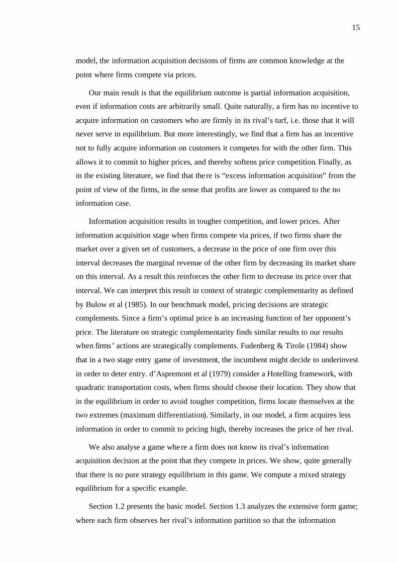
The blue and red lines show the partitions for si and sj respectively (the information

partition chosen by firm A and firm B).

Figure 1.3: Three possible segmentation scenarios

1.3. The Two-Stage Game

This game can be broken down into four different scenarios (figure 1.4). The first

scenario relates to the case when neither of the firms acquires information. The second

scenario represents the case where both firms acquire information. The third and fourth

scenarios represent the situation where only one of the firms decides to acquire

information.

Firm B

NI I

NI 1st Scenario 4th Scenario

Firm

A

I 3rd Scenario 2nd Scenario

Note: 3rd and 4th scenarios are symmetric

Figure 1.4: Four different scenarios for the two-stage game

1.3.1. Scenario One: Neither firm acquires information

The first scenario (the case of acquiring no information and therefore no price

discrimination) is easily solvable. In the equilibrium both firms charge uniform prices

( tPP BA == ), they share the market equally, and each firm’s profit is 2t

.

Firm A Firm B

Case 2:

Firm A Firm B Case 3:

Firm A Firm B Case 1:

22

1.3.2. Scenario Two: Both firms acquire information

In this scenario each firm acquires at least one unit of information that splits the

interval [0,1] into subintervals ([0,0.5] and (0.5,1]. Let us consider competition on an

interval that is a subset of [0,0.5] (given the symmetry of the problem, our results also

extend to the case where the interval belongs to (0,5,1]).

Let ]5.0,0[ˆ ⊆s and AIs∈ˆ , i.e. assume that s is an element of firm A’s

information partition. Consider first the case where s is the union of several elements

of B’s information partition, i.e. Un

iiss

1

ˆ=

= , for i =1,2,…n; This situation corresponds to

case 3 in figure 1.3.

Since firm A’s profits on the rest of the interval do not depend upon sP , she must

choose sP aiming to maximise her profit on s . By lemma 1, firm B’s profits on the

components of s do not depend upon her prices on this interval. Therefore, a necessary

condition for the Nash equilibrium is that:

a) A chooses sP to maximize her profits on s ,

b) B chooses P1 , … , Pn to maximize her profits on s .

An analogous argument also applies in cases 1 and 2.

From the utility function (1.1), the indifferent customer xi in each si = (ai-1, ai] is

located at:

Case 1: tPP

x ABi 22

1 −+= , for i =1; (1.5)

Case 2: tPP

x iABi 22

1 −+= , for i =1,2,…,n; (1.6)

Case 3: tPP

x AiBi 22

1 −+= , for i =1,2,…,n. (1.7)

In addition, these values for ix must lie in within the interval, i.e. the following

inequality should be satisfied for each ix :

iii axa ≤≤−1 , for i =1,2,…,n. (1.8)

23

Where 1−ia and ia are respectively the lower and upper borders of the segment si

and 5.00 1 ≤<≤ − ii aa .

In each segment is , the customers who are located to the left of ix buy from firm

A, and the customers to the right of ix buy from firm B. If ix (calculated in (1.5) or

(1.6) or (1.7)) is larger than the upper border ( ia ) all customers on is buy from firm A.

In this situation to maximise her profit, firm A will set her price for is to make the

customer on the right border indifferent. Similarly, if 1−< ii ax , firm B is a constrained

monopolist on is and will set her price to make the customer on the left border

indifferent.

Profits for the firms in each section of case 1 are:

−

−+= 022

1a

tPP

P ABAAπ , and (1.9)

−−−=

tPP

aP ABBB 22

11π . (1.10)

In cases 2 and 3, as mentioned before since the profit for each firm over si (i

=1,2,… ,n) can be presented only as a function of the prices over s , the maximization

problem is solvable for s independently. In case 2, firms’ profits on s are:

−

−+= −122

1i

iABiAiA a

tPP

Pπ , for i =1,2,…,n ; and (1.11)

−

−−=

−−−=

∑∑∑ =

== t

PnPn

aPtPP

aP

n

iiABn

iiB

n

i

iABiBB 2222

1 1

11

π . (1.12)

Similarly for case 3, the profits can be written as:

−−

+=

−

−+= ∑

∑∑

=−

=

=−

n

ii

A

n

iiB

A

n

ii

AiBAA a

t

nPPn

PatPP

P1

11

11 2222

1π , and (1.13)

−−−=

tPP

aP AiBiiBiB 22

1π , for i =1,2,…,n. (1.14)

24

So for cases 2 and 3, there are n+1 maximization problems on each s which should

be solved simultaneously.

Let IA and IB be two feasible information partitions for A and B respectively. Let I*

be the join of IA and IB, i.e. the coarest partition of [0,1] that is finer than either IA or IB.

Let s* be the element of I* is of the form [a,0.5), i.e. s* is the element that lies on the

left and is closest to the midpoint.

Lemma 2: s* is the only element of I* which lies to the left of 0.5 such that both

firms share the market. On every other element of I* which lies to the left of the

midpoint, all customers buy from firm A. 5

Proof: See appendix 1.A.

So both firms sell positive quantities only in the most right hand segment of firm

A’s turf and the most left hand segment of firm B’s turf.

This lemma has the following important implication. A firm has no incentive to

acquire information in its rival’s turf. For example if firm A acquires some information

on interval (0.5,1]; then firm B can choose a set of profit maximising prices where only

she shares this part of the market with firm A only on the very first segment on this

interval. So acquiring information on the interval (0.5,1] makes no difference on firm

A’s ability to attract more customers.

As a result of lemma 2, each firm sets a uniform price for all customers located in

her rival’s turf. Let us call these prices PRA and PLB. PRA is the price firm A sets for

[0.5,1] and PLB is the price firm B sets for [0,0.5). This price is set to maximize firm’s

profit in the only segment in the opposite turf that firm sells positive quantity in it. This

uniform price affects the rival’s price in her constrained monopoly segments. Thus the

pricing behaviour of firm A can be explained by these rules:

− In all segments on [0,0.5] except the very last one, s*, firm A is a constrained

monopolist. She sets her prices to make the customer on the right hand border of each

segment indifferent.

− On s*, the last segment to the right hands side of [0,0.5], firm A competes against

the uniform price set by firm B for the [0,0.5] interval.

5 The solution for the interval [0,0.5] can be extended to interval (0.5,1] where the solution is the mirror

image of the result on [0,0.5].

25

− On (0.5,1] she only can sell on the very first segment then sets her uniform price

for (0.5,1] in order to maximise her profit on that very first segment.

So, firm A’s partition divides [0,0.5] into n segments and she acquires no

information on (0.5,1]. Equivalently, firm B acquires no information [0,0.5] and has m

segments in her partition for (0.5,1].

We now solve for equilibrium prices. The prices for loyal customers in each side

would come from:

( )iLBiiA atPtaP −+=+ 1 , for 1,,2,1;1 −=≤≤− niaxa ii L , and

( )11 1 −− −+=+ iiBiRA atPtaP , for mnniaxa ii ++=≤≤− ,,2;1 L .

The prices for two shared market segments are represented by (recall from (1.A1)

and (1.A2)):

( )12132

−−= nnA at

P and ( )1232

1,1 −= ++ nBn at

P .

And the uniform prices for the opposite side could be written as:

BnRA PP ,121

+= and nALB PP21

= .

Then given the prices for these two segments prices for other segments can easily

be calculated as:

( ) ( )

( )

<<−

<<−

−=<<

−−

=

+

−−

−−

121

123

21

2132

1,,2,1;31

32

2

1

11

11

xat

xaat

niaxaaat

xP

n

nn

iini

A

L

; (1.15)

and

( )

( )

( )

++=<<

−+

<<−

<<−

=

−−+

++

−

mnniaxaaat

axat

xat

xP

iiin

nn

n

B

,,2;32

31

2

21

1232

21

0213

111

11

1

L

. (1.16)

26

The associated gross profits are (market shares for border segments are calculated

using the prices by (1.5)):

( ) ( ) ( )

−−+

−−+

−−−= ++−−

−

=−−∑ 2

131

.1232

132

.2132

31

32

2 1111

1

111 nnnn

n

iniiiA aa

taa

taaaatπ and

( ) ( ) ( )∑+

+=−+−++−−

−+−+

−−+

−−=

mn

niiniinnnnB aaaataa

taa

t1

1111111 32

31

221

32

.1232

21

31

.213

π .

After simplifying, the net profits are represented by (Note that each firm pays only

for the information in her own turf):

( ) Ann

n

iiiinnA aaaaaaat Γ−

−+

−+−−

−= +−

−

=−−− ∑

2

1

2

1

1

1111 2

192

21

98

231

32

2π , and (1.17)

( ) Bnn

mn

niiiinnB aaaaaaat Γ−

−+

−+−+−+−= +−

+

+=−−++ ∑

2

1

2

12

112

11 21

98

21

92

232

234

π . (1.18)

where ΓA, ΓB are the information costs paid by firms A and firm B in order to acquire

information.

If we want to follow the firm’s decision making process we can suppose that the

firm starts with only one unit of information and splitting [0.1] interval to [0,0.5] and

(0.5,1]. This first unit enables the firm to start discriminating on their half. Paying for

one more unit of information on their own half means that firm is now a constrained

monopolist on one part and should share the market on the other (i.e. for firm A, the

customers on [0,0.25] are her loyal customers and she shares the market on (0.25,0.5]

with firm B). In the loyal segment the only concern for the information acquisition

would be the cost of the information. Firms fully discriminate the customers depending

on the cost of information.

But there is a trade off in acquiring information to reduce the length of shared

segment. On one hand, this decision increases the profit of the firm through more loyal

customers. On the other hand, since her rival charges a uniform price for all customers

in the firm’s turf, the firm should lower the price for all of her loyal segments. Therefore

the second effect reduces the firm’s profit. These two opposite forces affect the firm’s

decision for acquiring a finer partition in the border segment. Proposition 1 shows how

27

each firm decides on the volume of the customer-specific information she is going to

acquire.

Proposition 1: Firm A uses these three rules to acquire information:

1-1. if 1610 ≤

tτ

, then firm A fully discriminates on [0,0.25]. The equal-size of the

segments on this interval in the equilibrium partition is determined by the information

cost.

1-2. Firm A acquires no further information on (0.25,0.5].

1-3. Firm A acquires no information on (0.5,1].

Proof: In order to avoid unnecessary complications, the first part of the proof has

been discussed in appendix 1.A. It shows that firm A should make a series of decisions

regarding to split the border segment (see figure 1.1). Starting form the pint of acquiring

no information on the left hand side, firm A acquires information in her own turf as long

as this expression is non-negative:

Γ−

−

−=∆ + 6

12

1127

21

2 2rkkAt

π , (1.19)

where k

na

=− − 2

121

1 is the length of the border segment,

r

21

is the preferred length of loyal segments (where

=

02 2

logτt

r 6), and

+−

=Γ2

12

0 krk

τ is the total information cost.

We follow this chain of decision makings, starting with n =1 (i.e. no initial loyal

segment for firm A). The procedure is that firm A starts with k = 1, if equation (1.19) is

non-negative then she decides to acquire information on [0, 0.5], splitting this interval

to [0, 0.25] and (0.25,0.5]. After this he is the constrained monopolist on [0, 0.25] and

the preferred length for all loyal segments is:

6 notation represents the floor function (or the greatest integer).

28

r

21 , where

=

02 2

logτt

r . (1.20)

After buying the first unit of information on [0, 0.5] (and consequently the preferred

units of information on [0, 0.25]) then firm A checks non-negativity of (1.19) for k = 2

and so forth.

Table 1.1 shows the chain of the first two decision statements. As it is clear the

value of the decision statement on the second row (and also for every k > 1) is always

negative.

Table 1.1: Firm A’s chain of decision statements

1−na na k Decision statement

0 21 1 0

4211

160 ≥

−

− τrt

r where

=

02 2

logτt

r

41

21 2 ( ) 0

82

21

61

320 ≥

−−

−− τrt

r where

=

02 2

logτt

r

The minimum value for r is 2 (the biggest possible length for a loyal segment is

1/4). It can be shown that the value of decision statement (equation (1.19) for k = 1) is

non-negative if and only if 1610 ≤

tτ

. It is clear the second row’s decision statement is

always negative. That means the length of the shared segment, regardless to the

information cost, equals 0.25. Assuming 1610 ≤

tτ

, then the preferred segmentation

scenario for firm A is to fully discriminate between [0,0.25] (the preferred segment

length in this interval is a unction of information and transportation cost) and acquiring

no information for (0.25,0.5]. ♦ QED

Each firm prefers to just pay for information in her own turf, and the segmentation

in the constrained monopoly part depends on the transportation and information cost.

The only segment in each turf that may have a different length is the border segment

and firms prefer to buy no information on their rival’s turf.

One of the findings in the proof of proposition 1 is the functional form of firms’

marginal profit of information in loyal segment. Equation (1A.16) shows that the

marginal profit of information in a loyal segment (dividing a loyal segment to two) is

29

( ) ( )

−

×=−− − 0

21 242

14

ττ kkiit

kaat where ai and ai-1 are the boundaries of the loyal

segment and kii aa21

1 =− − . As it is clear the marginal profit of information is

decreasing. Decreasing marginal profit guarantees that if the firm decides not to split a

loyal segment, there is no need to worry about the profitability of acquiring a finer

partition.

When the information cost is insignificant (τ0 =0) the preferred length of a loyal

segment goes to zero. In other words firms acquire information for every individual

customer on [0,0.25] and charges a different price for each individual based on her

location. In this case, in equation (1.19) k→ ∞, starting with an-1 = 0 and an = 0.5 and

based on the proposition 1 the chain of decisions for τ =0 is:

i) On [0,0.5], an-1 = 0 then equation (1.19) turns into 016

>t

and the result is to

acquire the first unit of information, and consequently acquire full information on

[0,0.25].

ii) On (0.25,0.5], an-1 = 0.25 then 0192

<−t

and the result is to acquire no further

information on (0.25, 0.5]. That means even when the information cost is insignificant,

the positive effect of acquiring more information in the interval of (0.25,0.5] is

dominated by the negative effect of falling the constrained monopolistic prices on

segments on [0,0.25].

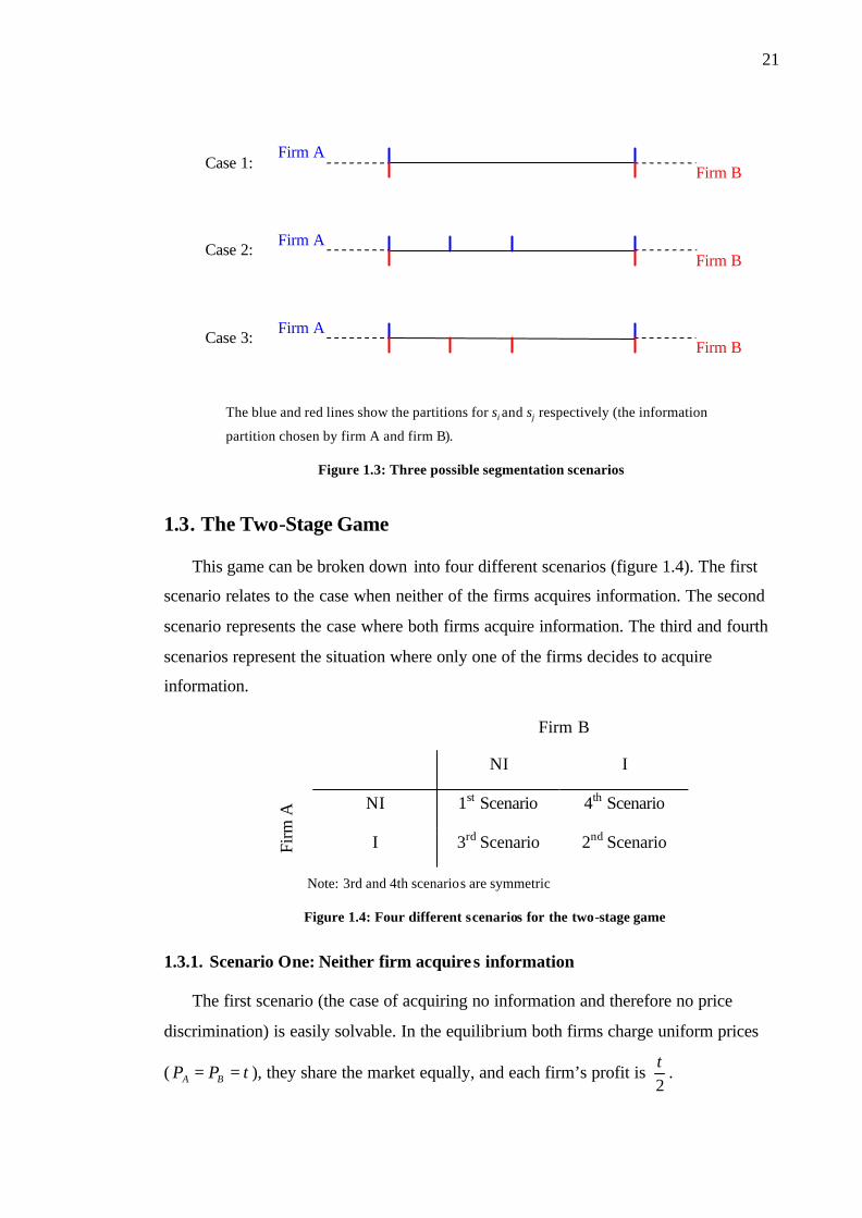
Figure 1.5 shows an example for an equilibrium strategy for firm A. Firm B’s

preferred strategy will be a mirror image of this example.

30

0 8

1 41 8

3 21 8

5 43 8

7 1

Figure 1.5: An example of the equilibrium strategy for firm A in the second scenario

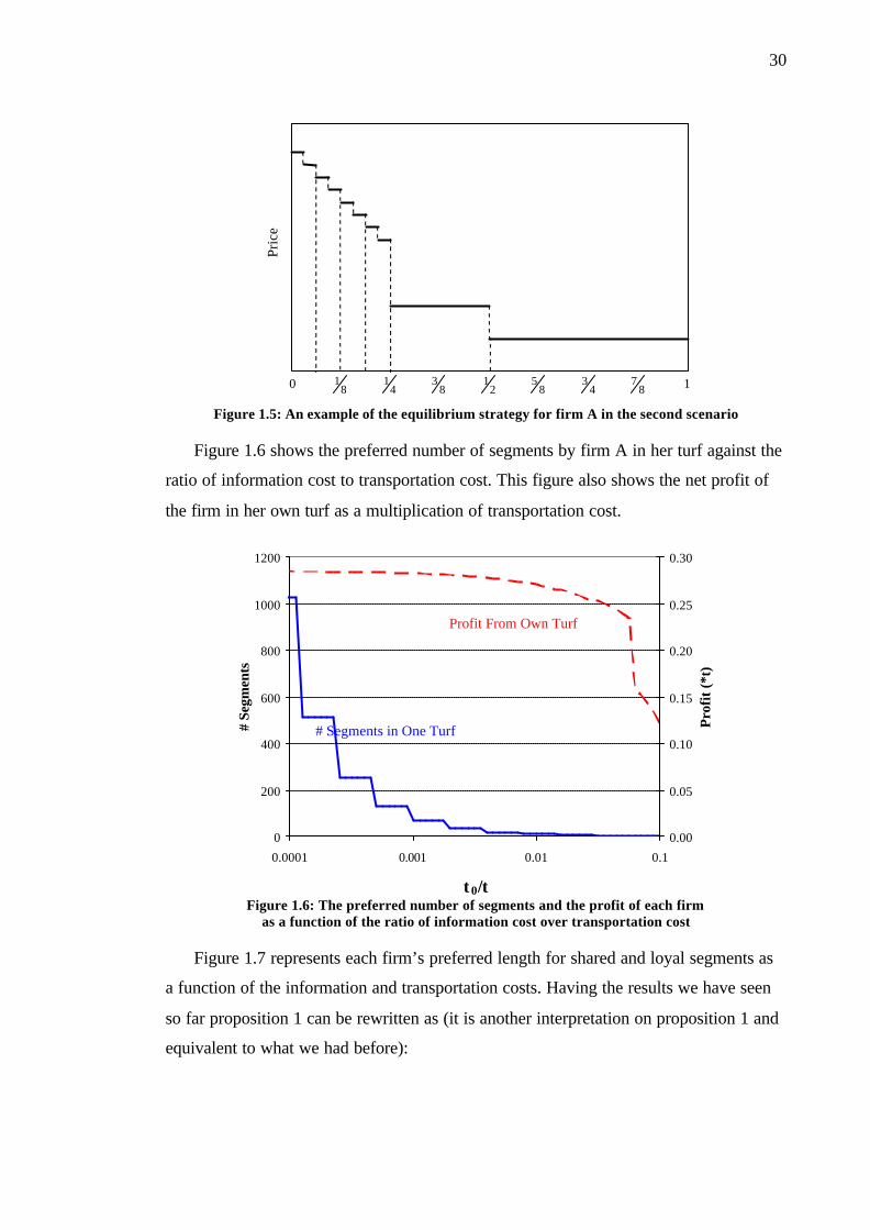
Figure 1.6 shows the preferred number of segments by firm A in her turf against the

ratio of information cost to transportation cost. This figure also shows the net profit of

the firm in her own turf as a multiplication of transportation cost.

0

200

400

600

800

1000

1200

0.0001 0.001 0.01 0.1

# Se

gmen

ts

0.00

0.05

0.10

0.15

0.20

0.25

0.30

Pro

fit (*

t)

Profit From Own Turf

# Segments in One Turf

τ0/t

Figure 1.6: The preferred number of segments and the profit of each firm as a function of the ratio of information cost over transportation cost

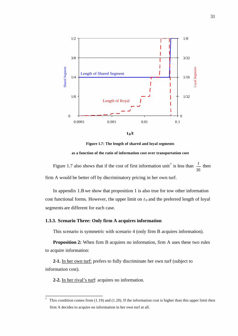
Figure 1.7 represents each firm’s preferred length for shared and loyal segments as

a function of the information and transportation costs. Having the results we have seen

so far proposition 1 can be rewritten as (it is another interpretation on proposition 1 and

equivalent to what we had before):

Pric

e

31

0

1/8

1/4

3/8

1/2

0.0001 0.001 0.01 0.1

Shar

ed S

egm

ent

0

1/32

1/16

3/32

1/8

Loya

l Seg

mne

ts

Length of Shared Segment

Length of Royal

τ0/t

Figure 1.7: The length of shared and loyal segments

as a function of the ratio of information cost over transportation cost

Figure 1.7 also shows that if the cost of first information unit7 is less than 16t then

firm A would be better off by discriminatory pricing in her own turf.

In appendix 1.B we show that proposition 1 is also true for tow other information

cost functional forms. However, the upper limit on τ0 and the preferred length of loyal

segments are different for each case.

1.3.3. Scenario Three: Only firm A acquires information

This scenario is symmetric with scenario 4 (only firm B acquires information).

Proposition 2: When firm B acquires no information, firm A uses these two rules

to acquire information:

2-1. In her own turf: prefers to fully discriminate her own turf (subject to

information cost).

2-2. In her rival’s turf: acquires no information.

7 This condition comes from (1.19) and (1.20). If the information cost is higher than this upper limit then

firm A decides to acquire no information in her own turf at all.

32

Proof: See appendix 1.A.

In this case firm B is not able of any discrimination and charges a uniform price for

all customers. If 81

161 0 ≤<

tτ

then firm A would prefer to acquire just one unit of

information in the left hand side [0,0.5] and the unique equilibrium prices are:

[ ]

( ]

( ]

∈

∈

∈

=

1,5.04

5.0,25.043

25.0,0

)(

xt

xt

xt

xPA and 2

)(t

xPB = .

If 1610 ≤

tτ

, then the proof of proposition 2 shows that firm B has no share from the

left hand side (even in the one next to 0.5 point) and only chooses her unique price to

maximize her profit on (0.5,1] interval. On the other hand, firm A would prefer to fully

discriminate the left hand side [0,0.5] and the preferred length of the segments are

determined by equation (1.20):

( ] [ ]

( ]

∈

⊂=∈

−

=−

1,5.03

5.0,0,67

)(1

xt

aasxtaxP

iiii

A and 32

)(t

xPB = .

Figure 1.8 shows a possible solution for this sub-game. As it is clear the indifferent

customer on [0,0.5] is the customer who is located exactly on 0.5. Then all the left hand

side customers buy from firm A. On the right hand side firm A’s market share is 1/3 and

the rest buy from firm B.

33

0 81 4

1 83 2

1 85 4

3 87 1

Figure 1.8: An example of the equilibrium strategy for the firms in the third scenario

1.3.4. Outcome of the Two-Stage Game

Figure 1.9 shows the strategic representation of the game when the information cost

is insignificant ( 00 →τ ). As it can be seen the game is a prisoners’ dilemma.

Firm B

NI I

NI 2

,2

tt 3625

,92 tt

Firm

A

I 92

,3625 tt

14443

,14443 tt

Figure 1.9: The outcome of the game when 00 →τ

Figure 1.10 represents firm A’s profit as a function of t0τ

. In each pair of strategies

the first notation refers to firm A’s strategy and the second one to firm B’s. If firm B

acquires information, firm A’s best response is to do so, irrespective of the information

cost. If the other firm acquires no information, the best response is to acquire

information if the information cost is sufficiently low. So if the information cost is

sufficiently low, the game becomes a prisoners’ dilemma and both firms would have a

dominant strategy to acquire information. This threshold is 039.00 ≈t

τ.

Firm A

Pric

e Firm B

34

0.10

0.20

0.30

0.40

0.50

0.60

0.70

0.0001 0.001 0.01 0.1

* t

( I , NI )

( NI , NI )

( I , I )

( NI , I )

τ0/t

Figure 1.10: Firm A’s profit for four different scenarios versus

the information / transportation cost ratio

Then if 039.00 >t

τ the game has two Nash equilibria: i) both firms acquire

information and ii) neither of the firms acquire information. If 039.00 ≤t

τ, the game is a

prisoners’ dilemma where information acquisition is the dominant strategy for both

firms. In this case we have excess information acquisition from the firm point of view.

Acquiring more information will lead to tougher competition and even in the limit,

when 00 →τ , will lead to about 40% decrease in firm’s profits.

Acquiring information has two opposite effects on firm’s profit. It enables the firm

to price discriminate and on the other hand toughens the competition. The latter effect

dominates the former and when both firms acquire information, they both worsen off.

Fixing the partitions for both firms, then pricings are strategically complement.

Given the outcome of this game, one might ask why do the firms not freely give

each other information about customers on their own turfs? The issue of collusion in

sharing the information in this game can be looked at from two different points of view.

Firstly, in the real world situation that our setting might be applied to sharing the

customer information with a third party is usually illegal. Fro example, Tescos –the

biggest supermarket in the UK with almost one third of the market share- has a huge

35

pool of specific information about its customers via its club-card scheme. However, it is

illegal for Tescos to share this information with other supermarkets.

Secondly, as it is showed in this section, information about the customers in the

other side of market has no strategic importance for the firm. Then even if the

information is available it makes no vital part in pricing decision. Since the outcome of

the game shows excessive information acquisition, one possibility for collusion is to

collude and not acquire information. However, as it was showed firms have incentive to

deviate from this agreement and acquire information.

1.4. The Simultaneous Move Game

In this game, firms cannot observe their rival’s information partition. It seems that

the two-stage game is able to offer a better explanation of the information acquisition

decision in a competitive market. Firms (especially in retailer market) closely monitor

their rival’s behaviour. Then it seems a reasonable assumption to consider that while

competing via prices, they are aware of the information partition chosen by their rival.

We will show that there is no pure strategy equilibrium in this game. Remember

that every strategy has two parts, the segmentation scenario and the prices for each

segment. To prove non-existence of pure strategy equilibrium, we show that for

different cases (regarding the information acquisition decision), at least one of the firms

has incentive to deviate from any assumed pure strategy equilibrium.

1.4.1. Case 1: None of the firms acquire information

The proof for the situation that none of the firms acquire information is trivial.

When both firms decide to buy no information, the outcome would be charging a

uniform price of t for both firms. It is clear that a firm has incentive to deviate from this

strategy and acquire some information when τ0 is sufficiently small.

1.4.2. Case 2: Both firms acquire information

Suppose there is a pure strategy equilibrium where both firms acquire some

information. Firstly we will show that in this equilibrium firms acquire no information

on their rival’s turf. Assume firm B acquires some information on [0,0.5]. In the

equilibrium every firm can predict her rival’s partition accurately. Therefore, based on

lemma 2, firm B makes no sale on every interval expect the final right segment on

36

[0,0.5]. Then the information on this interval is redundant for firm B. She can profitably

deviate, acquire no information on [0,0.5], and charge the same price for the entire

interval. Then in any pure strategy equilibrium firm B acquires no information on firm

A’s turf. We will therefore consider all different possibilities for firm A to acquire

information on [0,0.5]. Then we will show that in any candidate equilibrium at least one

of the firms has incentive to deviate (the fact that in the equilibrium each firm can

predict her rival’s strategy accurately is used).

i) No further information in [0,0.5]: The corresponding equilibrium prices at this

interval are

32

)(t

xPA = and 3

)(t

xPB = ; for [ ]5.0,0∈∀x .

It is trivial that firm A has incentive to deviate and acquire some information on the

left hand side. The information cost is not a binding constraint here. It has been shown

in the proof of proposition 1 that the constraint on whether to acquire some information

on [0,0.5) is more relaxed than acquiring any information in the first place (acquiring

information on [0,1]).

ii) Partial discrimination on [0,0.25]: This means firm A acquires the information

which splits [0,0.5] interval to [0,0.25] and (0.25,0.5] and some information (but not

fully discrimination) on [0,0.25] (and possibly some information on (0.25,0.5]). In the

equilibrium firm A knows that firm B sets a uniform price on the left hand side to

maximise her payoff from the very last segment on the right hand side of (0.25,0.5]

interval. Responding to this, as shown in proof of proposition 1, firm A has incentive to

fully discriminate on [0,0.25]. So a strategy profile like this cannot be an equilibrium.

iii) Full discrimination on [0,0.25] and no further information on (0.25,0.5]: As the

results of lemma 2 and proposition 1 show, if the information cost is sufficiently low in

equilibrium, firm A fully discriminates customers between [0,0.25] (subject to

information cost) and charges a uniform price for the section (0.25,0.5], and firm B

charges a uniform price for all customers on the left hand side in order to gain the most

possible profit from the customers on (0.25,0.5]. Now we want to investigate the

players’ incentive to deviate from this strategy profile.

Firm A has incentive to deviate from this strategy and acquire more information in

the information acquisition stage. Unlike the two-stage game, deviation from this

37

equilibrium and acquiring more information in the very last segment of the left hand

side (shared segment) doesn’t affect firm B’s price for the left hand side. Recalling

(1.A17) from the proof of proposition 1, firm A decides to acquire more information in

(0.25,0.5] if tτ

241

21

≥− or 641

≤tτ

. This is exactly the same upper bound for information

cost that satisfies firm A’s decision to acquire any information in the left hand side in the first

instance. That means if information cost is small enough to encourage firm A to acquire some

information in [0,0.5] interval, then firm A also has incentive to deviate from the

proposed strategy profile.

iv) Full discrimination on [0,0.5]: The corresponding equilibrium prices for the left

hand side are ((an-1,0.5] is the very last segment on the right where firm A acquires

information):

( ]

( ) ( ]

∈−

∈

−−

=

−−

−−

5.0,2132

,31

32

2)(

11

11

nn

iini

A

axat

aaxaatxP and ( )121

3)( −−= nB a

txP .

Firm B has incentive to deviate and acquire some information on the left hand side.

If firm B buys one unit of information on the left hand side then she can charge a

different price ( BP ) for [0,0.25]. The extra profit which she can achieve will be:

ττπ −

−−=−

−−−=∆ −−

BBn

Bn

BB Pt

PaP

atP

tˆ

2

ˆ

361ˆ

3125

2ˆ21

41 11 .

The first order condition results ta

P nB

−= −

361ˆ 1 and the corresponding extra

profit of ( ) τπ −−=∆ − 185.0 2

1t

an , which (considering the upper bound on information

cost for acquiring information in a firm’s own turf) gives firm B incentive to acquire at

least one unit of information of the left hand side.

Then the game has no equilibrium when both firms acquire information.

1.4.3. Case 3: Only firm A acquires information

Suppose this case has an equilibrium. In the equilibrium each firm can predict her

rival’s strategy including preferred partition; so firm A knows that in the equilibrium,

her rival can predict her chosen partition. We try to construct the characteristics of this

38

equilibrium. Since in the equilibrium firm B can predict her rival’s partition accurately,

then we can use some of the results that we had from the first game.

As seen in lemma 2, firm A knows if she acquires information in the right hand

side, firm B can prevent her of selling to any customer in the right hand segments

except the very first segment. Then firm A has no incentive to acquire information in

the right hand side.

As for the left hand side, proposition 2 shows that firm B knows that firm A can

gain the most possib le profit by fully discriminating. So firm B sets her price to just

maximise her profit from the only segment in her turf and firm A fully discriminate the

left hand segment.

An equilibrium for this case should have these two characteristics:

1- In the right hand side, firm A (the only firm who acquires information in this

scenario) buys no information. Then there is only one segment (0.5,1] and the prices

would be 32t

P RHSA = and

34t

PB = .

2- in the left hand side, firm A fully discriminates subject to information cost given

the firm B’s uniform price.

Now we want to investigate firm A’s incentive to deviate from this equilibrium.

Given firm B’s uniform price, if firm A deviates and acquires just one unit of

information in the right hand side his marginal profit would be the difference between

his equilibrium profit over (0.5,1] and the deviation strategy profit over (0.5,0.75] and

(0.75,1]. Then the deviation profit can be written as ( LAP the price charged for the left

sub-segment and RAP the price for the right sub-segment):

τπ −

−−

+

−=

41

234

234

t

Pt

Pt

Pt

P

RA

RA

LA

LA

RHSA . (1.21)

Solving the FOCs, the first part of (1.21) exactly gives firm A the same profit as the

supposed equilibrium. If the second part of the profit is greater than the information

cost, then firm A has incentive for deviation. From the FOC 125t

P RA = , the marginal

profit of deviation is:

39

ττπ −=−

−=∆

28825

41

2411

125 ttRHS

A .

If 087.028825

≈≤tτ

firm A has incentive to deviate and acquire at least one unit of

information in the right hand side. This condition is more relaxed than the condition

calculated in section 1.3.2 for acquiring information in her turf at all. That means if the

information cost is low enough that firm A decides to acquire information in the left

hand side, in the first place, she has incentive to deviate from any equilibrium strategy

that constructed for this case.

1.4.4. Outcome of the Simultaneous Move Game

The major result of studying the simultaneous move game is the non-existence of

equilibrium in pure strategies. Therefore the only possible equilibrium of this game

would be in mixed strategies. Considering that each pure strategy consists of an

information partition and a pricing function measurable with the chosen information

partition, one can imagine that in general there are many possible pure strategies. This

makes finding the mixed equilibrium of the game a difficult task. In appendix 1.C, we

investigate the existence of a mixed strategy equilibrium through a simple example

where the number of possibilities are exogenously restricted.

1.5. Comparing the Two-Stage Game with the Multi-Store Example

In this section we compare our model with the spatial competition among multi-

store retailers. The spatial competition model has been studied in several papers (Teitz

(1968), Martinez-Girlat & Neven (1988), Slade (1995), Pal & Sarkar (2002)). Consider

two retailers, initially each with one store located at the two ends of [0,1] interval. They

have the option to open new stores alongside the line. Opening a new store enables the

firm to price discriminate, by charging different prices at different stores. In a two stage

setting, first each firm decides whether to open their new branch and then firms compete

via prices.

Spatial competition models can also be described as introducing new models in a

differentiated market where customers have different tastes. Assume there are two

brands of car (say Honda and Toyota) and the customers are uniformly located on the

interval between these two brands based on their tastes. If a customer’s location is

40

closer to Honda, he likes Honda more. The customer who is located at the mid-point is

indifferent between two brands.

So the problem for car makers is to produce different models alongside the line to

be able to price discriminate. For example, Toyota might want to make some changes to

their existing model and making a new model more like Honda products to attract some

of Honda customers. Making these changes for the car maker bears a relatively small

cost. In a two stage setting, firms first choose their models and then compete via prices.

The information acquisition model is different from this model. In the information

acquisition model the products offered to all customers are identical; but in the multi-

store model, firm is able to charge different prices by offering different products. In case

of considering the model in a spatial context, the difference is the location of stores. In

the information acquisition game the pattern of transportation cost was unaffected by

the price discrimination practice. In the multi-store model, opening each store

potentially reduces the transportation cost for some of the customers who shop at new

stores.

In order to demonstrate this we illustrate an example of spatial competition which

has similarities to our model. Assume two retailers A and B each with one store located

at points 0 and 1 respectively. In the first stage they each might decide whether to open

a new store or not. Retailer A has the option to open her new store at 0.25 and retailer B

can open her new store at 0.75. After making this decision, both firms observe their

rival choice. The game proceeds to the next stage where firms compete in prices.

Customers are uniformly distributed on [0,1]. Each customer buys at most one unit of

good and her utility is tdPVU −−= where V is her reservation price, P is the price

she paid, t is the unit cost of transport, and d is the distance to her chosen store. Firms’

marginal costs are equal, normalised to zero and the cost of opening a new store is c.

Note that in this game each firm charges a uniform price for all customers at each

store. The only option for a firm to price discriminate is to open a new store.

The game has four sub-games as it is shown in figure 1.11. We solve each sub-

game and then characterise the sub-game perfect equilibrium.

41

Firm B

Not Open Open B2 @ 0.75

Not Open 1st sub-game 4th sub-game

Firm

A

Open A2 @ 0.25 3rd sub-game 2nd sub-game

Third and forth Sub-games are symmetric.

Figure 1.11: The multi -store retailer game

1.5.1. First sub-game; None of the firms opens a new store

The equilibrium in this sub-game is trivial. Both firms charge uniform prices

( tPP BA == ), they share the market equally, and each firm’s profit is 2t

.

1.5.2. Second sub-game; Both firms open a new store

Figure 1.12 shows the spatial representation of this sub-game. We call stores

located at 0 and 0.25, A1 and A2 respectively. Similarly stores located at 1 and 0.75 are

called B1 and B2.

Figure 1.12: The 2nd sub-game of the multi-store retailer game

The utility of the customer who is located at x is (Pi is the price charged by store i):

( )

( )

−−−

−−−

−−−

−−

=

11

22

22

11

143

41

BfrombuyssheifxtPV

BfrombuyssheifxtPV

AfrombuyssheifxtPV

AfrombuyssheiftxPV

xU

B

B

A

A

. (1.22)

We restrict our search for equilibrium to symmetric equilibria. In any symmetric

equilibria 11 BA PP = and 22 BA PP = . Based on this, we can conclude that in the

equilibrium customers in each of the segments ([0,0.25], (0.25,0.75], and (0.75,1]) shop

at one of the two stores located at the two ends of that segment. For example customers

on [0,0.25] shop either at A1 or A2. It is trivial that customers on this interval have no

incentive to shop at either of firm B’s stores, since it only increases their transportation

A1 A2 B2 B1

0 x1 0.25 x2 0.75 x3 1

42

cost. The same argument is true for interval (0.25,0.75], if in the equilibrium

421t

PP AA −≥ . This condition guarantees that customers located on (0.25,0.75] has no

incentive to travel to either of stores located at 0 and 1.

Assume x1, x2, and x3 (see figure 1.12) are the location of indifferent costumers in

each segment. Considering our assumption and equations (1.22), the locations of

indifferent customers are:

tPP

x AA

281 12

1−

+= , (1.23)

tPP

x AB

221 22

2−

+= , and (1.24)

tPP

x BB

287 21

3

−+= . (1.25)

Firm A’s total profit from both stores is:

( ) cxxPxP AAA −−+= 12211π . (1.26)

Substituting from (1.23) and (1.24) into (1.26); and calculating the first order

conditions, the best response prices for firm A are8:

tPP AA 81

21 += and 22

122

tPP BA += .

Following a Similar procedure for firm B the best responses for firm B are:

tPP BB 81

21 += and 22

122

tPP AB += .

Solving these two set of best responses together, the location of indifferent

customers (x1, x2, and x3) are 161

, 21

, and 1615

. The equilibrium prices are:

tPP BA 89

11 == and tPP AB == 22 . (1.27)

And the firms’ equilibrium profit is:

ctBA −==12865

ππ . (1.28)

8 The second order condition satisfies the maximum that this solution is a maximum.

43

Prices in (1.27) satisfy the condition that we need for this equilibrium

(421t

PP AA −≥ ). As it can be seen in (1.27) in this sub-game the competition is limited

to the middle segment. The competition on this segment has the same pattern as the 1st

sub-game and the outcome in this segment is similar to the outcome of the 1st sub-game

where the prices are equal to t and firms share the market equally.

The possibility of a global deviation by firms should be investigated. The possible

deviation strategies for firm A are (given firm B’s prices are fixed as (1.27)):

i) Reduce PA2 (and consequently PA1) in order to capture a higher share from the

right hand side with the possibility of attracting some of the customers on

(0.75,1] interval.

ii) Increase PA2 (and consequently PA1) in order to increase her profit on [0,0.25]

interval.

iii) Ignore A2 store and try to maximise her profit only through A1.

It is investigated and none of the above alternative strategies increases firm A’s

profit. Then the equilibrium discussed here is the unique symmetric equilibrium of this

sub-game.

1.5.3. Third sub-game; Only firm A opens a new store

Figure 1.13 shows the spatial representation of this sub-game. In this sub-game firm

A has two stores located at 0 and 0.25 and firm B has one store located at 1.

`

Figure 1.13: The 3rd sub-game of the multi-store retailer game

We assume that in the equilibrium customers in each of the segments ([0,0.25] and

(0.25,1]) shop at one of the two stores located at the two ends of that segment. After

finding this equilibrium we prove that this is a global equilibrium.

Assume x1 and x2 (see figure 1.13) are the location of indifferent costumers in each

segment. Considering our assumption and equation (1.22), the locations of indifferent

customers are

A1 A2 B

0 x1 0.25 x2 1

44

tPP

x AA

281 12

1−

+= and (1.29)

tPP

x AB

285 2

2−

+= . (1.30)

Firm A’s total profit has the same form as (1.26). By substituting from (1.29) and

(1.30) into (1.26); and calculating the first order conditions, the results are (these are the

best response function for firm A)

tPP AA 81

21 += and tPP BA 85

21

2 += .

Firm B’s total profit is:

( )21 xPBB −=π . (1.31)

Substituting from (1.30) into (1.31); and calculating the first order condition, the

result for firm B is

tPP AB 83

21

2 += .

Solving these two set of best responses together, the location of indifferent

customers are 161

and 2413

. The equilibrium prices are:

tPA 2429

1 = , tPA 1213

2 = , and tPB 1211

= . (1.32)

And the firms’ equilibrium profits are:

ctA −=1152685

π and tB 288121

=π . (1.33)

Prices as it can be seen in (1.32) show that in this sub-game, the competition

between the firms are limited to [0,0.75].

The deviation possibilities for the firms again fail to improve the profit. Then it is

the unique equilibrium of this sub-game.

1.5.4. Outcome of the multi-store game

Figure 1.14 summarises the outcome of the four sub-games. For different values of

c the sub-game perfect equilibrium has different characteristics:

45

i. If tc128

1≤ , then both players have a dominant strategy to open the new store.

But the game is not a prisoners’ dilemma. Opening the new stores by both

firms improves the profit for both firms.

ii. If tct1152101

1281

≤< , then it is still a dominant strategy to open the new store for

both firms; however the game is a prisoners’ dilemma.

iii. If tct1152109

1152101

≤< , then the game has two asymmetric equilibria, when one

firm opens the new store and her rival does not.

iv. If ct <1152109

, then each firm has a dominant strategy not to open the new store.

Firm B

Not Open Open B2 @ 0.75

Not Open 2t

, 2t t

288121

, ct −1152685

Firm

A

Open A2 @ 0.25 ct −1152685

, t288121 ct −

12865

, ct −12865

Figure 1.14: The payoffs in the multi-store retailer game

This game - like the information acquisition game - has a dominant strategy of

opening the second store conditional on tc1152101

< . However, the game is not a

prisoners’ dilemma. In fact for different values of c, the game has different

characteristics. Note that in the information acquisition game if information cost was

less than a threshold, game was a prisoners’ dilemma.

We now try to explain intuitively what happens as the number of firms rises in this

model.

Assume that firm A can open stores in the interval [0,0.5), while firm B can open

stores in the interval (0.5,1]. We define the mid-interval as [a,b] where a and b are the

location of the two closest stores to the mid-point respectively belonging to firm A and

firm B. As our previous example of four stores (two stores for each firm) showed, the

pattern of competition on the mid- interval is similar to the game with only one store for

46

each firm. That is, the two stores on both sides of the med- interval compete for

customers, just as the two stores located at 0 and 1 did in the original game. Thus,

similar intuition suggests that when firms can open many stores, competition is

restricted to the mid- interval. Other stores located on other intervals are able to charge a

higher price. One can solve a free entry equilibrium in this case where firms can open

many stores, but each additional store incurs a fixed cost.

Intuitively, this setup seems different from the information acquisition game. Since

stores away from the mid-interval are able to charge a higher price. Therefore in one

hand, firms would like to open stores closer to mid-point to push the competition further

away from the segments they are constrained monopolist on. On the other hand, firms

would like to open stores away from the mid- interval and where they have more

monopoly power to increase their profit. The factor that limits the number of stores is

the cost of a running new store. Thus opening new stores may allow firms to relax

competition, unlike in the information acquisition case, where competition is increased.

1.6. Summary and Conclusion

This chapter has analysed a model of information acquisition by firms, where

information allows firms to price discriminate. Our benchmark model is one where

information acquisition decisions are common knowledge at the time that firms compete

via prices. We show that information acquisition increases price competition and

reduces profits, so that we have an outcome similar to a prisoners’ dilemma. Our second

main finding is that firms acquire less information as compared to a monopoly situation,

since this softens price competition.

By introducing information cost (and as a consequence segmentation scenario), the

third-degree price discrimination problem can end up neither on fully discrimination

policy nor on non-discrimination decision. Depending on the cost of every unit of

information, every firm needs to answer two questions: how should I discriminate (what

is the preferred length of every segment) and what is the best price to charge for every

specified customer. The result would be a partially discrimination policy.

The two-stage game is a prisoners’ dilemma which in equilibrium, firms acquire

excessive information. Firms also prefer to discriminate partially. Our results show that

there is a trade-off in acquiring more information. It improves firms’ performances in

47

terms of profit by enabling them to price discriminate. On the other hand, acquiring

more information tends to make the competition between the firms more fierce.

Tougher competition drives the prices down and ultimately decreases firms’ profits.

Our results demonstrate how decreasing marginal profit of information limits firms’

willingness to acquire more information. Furthermore, in equilibrium –regardless of the

cost of information- firms do not have incentive to acquire information on their rival’s

turf. Acquiring information in a firm’s own turf is also restricted. Extra information in

this area makes firms profit to fall as result of tougher competition.

We have also analysed a model where information acquisition decisions are not

observed by the rival firm. In this game, there is no pure strategy equilibrium. We solve

for a mixed strategy equilibrium for a simple example, where firms have restricted

information acquisition possibilities

Appendix 1.A

Proof of lemma 2: Since the firms’ profit on s can be written as a function of the firms’

prices on s and the segments associated with that (si ; i =1,2,… ,n), firms solve the

maximization problem for s independently of its compliment. We solve the problem for

each possible segmentation situation

Case 1:

By solving the first order conditions ( 0=∂∂

A

A

Pπ

, 0=∂∂

B

B

Pπ

), market shares, prices, and

profit of firms is calculated. By applying the FOC to (1.9) and (1.10) and solving them

simultaneously, firms’ prices are:

( )1423 01 +−= aat

PA , and (1.A1)

( )1243 01 −−= aat

PB . (1.A2)

By substitution the prices from (1.A1) and (1.A2) into (1.5), the location of marginal

customer in every segment is derived:

( )12261

01 ++= aax . (1.A3)

48

In the segments that both firms sell positive quantities, the prices should be non-negative

( 0≥AP , 0≥BP ) and the marginal customer should be located within the segment

( 10 axa ≤≤ )9. From the information acquisition technology at the definition of the model,

every two consecutive breaking points (the borders of each segment) have the following form:

p

ka

212

0−

= , q

la

212

1−

= where ℵ∈qplk ,,, . (1.A4)

And also the length of segment is represented as10:

raa

21

01 =− where qpr ,max= . (1.A5)

Solving the restrictions, the results are:

i) If qp > then the restrictions hold only for 21

1 =a ; both firms sell positive quantities in

the segment located exactly at the left hand side of the middle point11.

ii) If qp < then the restrictions hold only for 21

0 =a ; both firms sell positive quantities in

the segment located on the right side of the middle point.

iii) qp = is impossible, it is equivalent with a segment of length zero.

In this case, market sharing takes place only for two segments located around 21

.

9 Obviously, the price restrictions and the location restrictions are equivalent.

10 This definition covers all amounts of 0a except 00 =a . That can be solved as: 11 6120 aa <+< then

141

a< . Since 41

21

01 >=− raa and 00 =a then 21

1 =a is the only possible upper border of a

segment with positive demand for both firms.

11 Proof: pp

kaa

22

21

01 =+= . Substitute in (1.A1) and (1.A2), and apply in the price restrictions:

21

2 2 −> −pk , and 12 2 +< −pk . Since ℵ∈k then 22 −= pk , and 21

1 =a . The proofs of other two cases

are quite similar.

49

Case 2:

In case 2 by solving the first order conditions on s ( 0=∂∂

iA

iA

Pπ

, 0=∂∂

B

B

Pπ

; ni ,,2,1 L= )

market share, prices, and profit of firms is calculated. By applying the FOC to (1.11) and (1.12)

and solving them simultaneously the firms’ prices are:

+−−+

= −

−

=∑

132

3 1

0

1

1i

n

iin

iA an

aaat

P for ni ,...,2,1= and (1.A6)

−−+= ∑

−

=naaa

nt

Pn

iinB 0

1

1224

3. (1.A7)

The solution is started from the first segment (s1 which is the first segment in the very left

hand side of s ) and shows that the location for indifferent customer does not satisfy

110 axa ≤≤ then the maximization problems are reduced to n. This procedure continues to the

most right hand side segment with a couple of FOCs and problem reduces to the problem solved

in case 1.

−++−+=

−+= ∑

=nnaaaa

ntPP

xn

iin

AB 2361

21

221

01

01

1 .

Define 0aaii −=λ then:

+++= ∑

=

n

iinn

ax1

01 61

32

61

λλ .

To be credible we should have 101 λ+< ax and simultaneously 0>BP then:

101

0 61

32

61

λλλ +<

+++ ∑

=a

na

n

iin , (1.A8)

and from (1.A7): 020

1

>−++ ∑=

nna

n

iin λλ (1.A9)

After simplifying (1.A8):

0321

21

11

0 <−

++− ∑

=λλλ

n

iinn

a . (1.A10)

And from (1.A9):

50

−>+ ∑

=0

1 21

ann

iin λλ .

Define 021

≥=− γna :

RHS of (1.A10) ( ) 1100 323

321

221

λγλλ −+=−

−+−> na

nn

a .

For every n>1 ; 12λλ ≥n then (1.A8) and (1.A9) cannot be held simultaneously.

Then we showed for every n>1 in the first segment firm A is a constrained monopolist. For

the ith step if n>i it is easy to show that these two constraints turn to this form (with in −+ 2

FOCs):

( ) ( ) ( ) ii

n

ijjin

iABi ainainaaa

intPP

x <

−+−−+++−

−++=

−+= −

=− ∑ 1213

161

21

221

11 ,

and 0>BP è 021

1 >−+

−−+∑=

−

n

ijijn

inaaa .

After simplifying:

( ) 012

13

23

21

110 <

+−

−++−+− ∑

=−−

n

ijjinii in

a λλλλλ , (1.A11)

and ( )∑=

−

−−+>+−

n

ijjin ain 01 2

11λλλ . (1.A12)

Then

The RHS of (1.A11) ( ) ( )γλλλλλ ++−=−−

−> −− 110 2

23

223

21

23

iiniia .

For i<n; ( )121

−+≤ ini λλλ Then (1.A11) cannot be hold, supposing (1.A12) holds.

This procedure continues until the FOCs reduce to 2 conditions and the problem transforms

to the problem has been solved in case 1.

51

Case 3:

In this case by solving the first order conditions for each segment ( 0=∂∂

A

A

Pπ

, 0=∂∂

iB

iB

Pπ

;

ni ,,2,1 L= ) market shares, prices, and profit of firms is calculated. By applying the FOC to

(1.13) and (1.14) and solving them simultaneously the firms’ prices are:

−−+= ∑

=0

1

4243

aaannt

Pn

iinA and (1.A13)

−−

+−=∑

=

n

aaaa

tP

n

iin

iiB

01

2213

3 for ni ,...,2,1= . (1.A14)

Again for the first segment:

−+++−+=

−+= ∑

=

nnaaaant

PPx

n

iin

AB 232261

21

221

11

01

1 .

Then we should have:

11

01

1 2261

261

aaaan

ax

n

iin <

+−++= ∑

=

.

Or equivalently:

02261

261

10

11 <

+−+−= ∑

=

n

iin aaa

na

x .

Again consider 0aaii −=λ then:

0221

23

23

21

01

10 <

++−+−− ∑

=

nan

a n

iin λλ

λ,

or:

0221

23

21

1

10 <

+−+−− ∑

=

n

iinn

a λλλ

. (1.A15)

52

Now, we show that the minimum amount the right hand side is not negative. It is easy to

show that the minimum of

+− ∑

=

n

iin

1

2 λλ is nnλ

121

−− and the maximum amount of 1λ is

2nλ

then (recall 021

≥=− γna ):

The RHS of (1.A15) )21

41

(22

321 1

0 nnnn

nna −+=−−−≥ λγ

λλ.

Then as long as n > 1 (1.A15) is not valid and in the first segment firm A is a constrained

monopolist. For the ith step if n > i it is easy to show that firms’ preferred price for each section

turn to this form:

( )

−−++−

+−= ∑

=04241

13aaain

int

Pn

ikknA and

+−

−−+−=

∑=

1

2213

3

0

in

aaaa

tP

n

ikkn

jjB for ij ,...,2,1= .

The location of indifferent customer for the last segment could be calculated as follow

(with in −+ 2 FOCs):

−+−−++++−

−++=

−+= ∑

=

)1(2)1(322)1(6

121

221

0 inainaaaint

PPx i

n

ikkn

AiBi .

By following a procedure as before it could be shown that ii ax ≥ as long as n > i and

0≥γ . It means in this case we again end up with a problem similar to case 1 and firms share

the market in only the very two extreme segments in the middle. ♦ QED

Proof of proposition 1: Firm A’s decision to acquire one more unit of information to split the

segment between any two already known consequent points can be considered as one of these

two cases (note it is already proved that firm A has no incentive to acquire information on the

right hand side).

i) Acquisition of one more information unit for dividing one of the first n-1 segments to two

equal sub-segments. Since firm A splits one of her loyal segments to two loyal sub-segments,

then the marginal profit of this segmentation for the firm A is (k

ii aa

=− − 2

11 where k > 1):

53

( ) ( )kaaaaaaaaaa

aat iiiiiiiiii

iiA τπ −

−+

−

+

+

−

+

−−=∆ −−−−−

11111

2222 .

Where the first two parts are the amounts of extra profit that firm gets from the two sub-

segments and the third part represents the similar amount for the original segment that should be

subtracted. After simplifying:

( ) ( )kaat

iiA τπ −−=∆ −2

14. (1.A16)

This shows that firm A’s demand for more information and consequently more precise

price discrimination in this part (the first n-1 segments) continues as far as the length of pre-

final segments satisfies:

( )tk

aa iiτ

21 ≥− − .

or equivalently (by substituting k

ii aa

=− − 2

11 and ( ) kk

20τ

τ = ):

02 4

logτt

k ≤ . (1.A17)

This result means the firm has incentive to split a loyal segment, if k satisfies this

inequality. This is equivalent of minimum length which the firm has incentive to split the

interval if the loyal interval is bigger than this minimum length. Therefore, the preferred length

of a loyal segment is 1

21

+

k

.

We also can conclude that the preferred length for every firm’s loyal segment in her turf

does not depend on the location of the segment and depends only on the transportation and

information costs and considering (1.A17) and the fact that 0Uℵ∈k then the preferred

length for a loyal segment is:

r

21 where

=

02 2

logτt

r . (1.A18)

notation represents the floor function (or the greatest integer). It is clear since it is about the

length of a loyal segment then the minimum acceptable value for r is 3.

ii) Acquisition of one more information unit for dividing the nth segment to two equal sub-

segments. Since firm A splits one shared segment to two sub-segments which the left one will

54

be a loyal segment and the right one is a shared segment with her rival, then the marginal profit

of such segmentation for the firm A is (k

na

=− − 2

121

1 ):

( )katata

aa

t

aat

aat

n

nn

n

n

n

n

n

n

A

τ

π

−

−−

+−+

+

−+

−

−

+−

−+

=∆

−

−−

−

−

−

−

−

−

2

1

2

11

1

1

21

2

1

1

1

21

98

221

21

98

241

221

2

221

32

221

34

,

or ( )kt

at

at

kkknnA ττπ −

−

×=−

−−

−=∆ −− 2

121

2321

621

3 1

2

1 .

For ∀k, this marginal profit is negative and shows the firm A’s profit reduces by acquiring

one more unit of information in this part regardless of information cost. But we should consider

that the left sub-segment created after this information acquisition all are loyal customers now

and the possibility of making extra profit by using constrained monopoly power on this sub-

segment should be considered. This possibility can be investigated. Consider (1.A18), assume

the preferred length of loyal segment is r

21 where 3

2log

02 ≥

=

τt

r . It is clear acquiring

information in this interval is only profitable if r > k; however the following result is true for

any value of r. By adding the profit of this chain of segmentation the net profit of segmentation

in the nth segment, (an-1,½], is:

Γ−

−−

+−+

−+

−−

−

+−

−+

=∆

−

−

=

−−

−

−

−

−

−

∑

2

1

2

1

2

1

11

1

21

2

1

1

1

21

98

221

21

98

241

2241

21

2

221

32

221

34

n

n

i

nrn

nr

n

n

n

n

A

atat

aia

at

aat

aat

r

π

,

or

55

Γ−

−−

−

−=∆ −−+ 1

2

12 21

61

21

21

127

nnrA aatπ ;

and finally

Γ−

−

−=∆ + 6

12

1127

21

2 2rkkAt

π (1.19)

where the information cost is

( ) ( ) ( )( )

+−

=+=+=Γ ∑∑−

+=

+−−

+=

+−

21

222

22 0

1

1

01

01

1

1 krik k

r

kii

ki

k

r

ki

ki τττττ ,

k

na

=− − 2

121

1 , and

=

02 2

logτt

r .

If the net profit calculated by (1.19) is negative then the segmentation in the nth segment is

not profitable for firm A. Then the segmentation in the shared segment in firm A’s turf is

preferred by her as far as (1.19) is non-negative which because of it is importance is discussed

in the main body of paper. ♦ QED

Proof of proposition 2:

We know that the firms only share the customers on the two border segments. Suppose

Firm A acquires information in her own side such that the last left hand segment is (a,0.5], and

as it has been proved in proposition 1 she has no incentive to pay for information in the right

hand side. Then the maximization problems that should be solved simultaneously are:

Firm A’s profit for (a,0.5]:

−

−+= a

tPP

P LABLALA 22

1π .

Firm A’s profit for (0.5,1]:

−

=tPP

P RABRARA 2

π .

Firm B’s profit for (a,1]:

−−

−=t

PPPP RALAB

BB 22

21

π .

Solving the FOCs and the results are:

ta

PB

−=

321 , t

aPLA

−=

67

43 , and t

aPRA

−=

641 .

And the locations of indifferent customers in these two segments are:

125

83 a

xL += and 128

5 axR −= .

56

These values should satisfy 0>iP , 21

<< Lxa , and 121

<< Rx .

Since if 3.0>a , then xL will not satisfy its condition. Therefore, for 3.0>a , firm B cannot

gain from the left hand side. That means if firm A decides to split up (0.25,0.5] then firm B just

set her price to gain the most possible profit from the right hand side.

Then we compare the profit of firm A for different possible decisions (the profits are easily

calculated similar to the result of lemma 2)12:

1- No information in left hand side: 0165

τπ −=t

A ,

2- Fully discriminate

41

,0 : ( )23

21

576241 0

2

τπ

+−

−= +

rtrA , and

3- Fully discriminate

21

,0 : ( )2

322

13625 0

2

τπ

+−

−= +

rtrA ;

where

=

02 2

logτt

r .

If rt 96

530 ≤τ

then the third one provides the largest profit for firm A (the profit on the first

case exceeds the third one only when 576101

≥tτ

which is larger than 161

the upper bound of

information acquisition decision calculated in proposition 1); then she prefers to fully

discriminate all the left hand side. In this case firm B’s profit equals to 92t

. ♦ QED

Appendix 1.B

In this appendix we replace our assumed form of information cost function with two

alternative functional forms. Then we represent the changes to the outcomes of the model as a

result of these changes. Note that lemma 1 and lemma 2 are true regardless of the information

cost sequence. We focus on how the changes to equation (1.2) changes proposition 1,

proposition 2, and the outcome of two-stage game. The result is that firms strategically behave

in the same way. Only the length of the loyal segments and the thresholds on information cost

calculated in the proofs are different.

Our two alternative information cost functions are: 12 The length of the loyal segments is calculated with the same rule as equation (1.20).

57

i) constant information cost: ττ =)(k for ∀k.

ii) information cost with general functional form of:

0)( τατ kk = , for ∀k. (1.B1)

The other two information cost functions (equation (1.2) and the constant information cost)

are specific cases of (1.C1).13

In order to emphasis the changes, we add notations c and g to each equation number that

changes for constant and general information cost functions respectively.

Constant information cost:

Assume equation (1.2) is replaced by:

ττ =)(k for ∀k.

Proposition 1:

The proposition 1 is true for this case. Only because of the change in information cost

function to a linear cost function the limit on the first rule is different:

Recall equation (1.A16) the marginal profit of acquiring a unit of information in a loyal

segment:

( ) ( )kaat

iiA τπ −−=∆ −2

14. (1.A16)

This equation gives us the limit to the which is now (by substituting k

ii aa

=− − 2

11 and

( ) ττ =k ) equation (1.A17) changes to:

k

21 where

τ4log

21

2t

k ≤ . (1.A17.c)

Then the preferred length for a loyal segment is:

r

21 where

=

τt

r 2log21 . (1.20.c).

13 We decided to have the special case of

21=α in the main body of paper, since calculating the closed

form of some equations which helps to demonstrate our results is more complicated for the general

functional form of (1.3).

58

The marginal profit of a unit of information on the shared border segment with the length of

k

21 is (note the marginal profit has the same format and only the information cost and the

preferred length of the loyal segment are different):

−

−

−=∆ −

+ τπ krrkkA

t2

61

21

127

21

2 2 . (1.19.c)

where k

na

=− − 2

121

1 , and

=

τt

r 2log21 .

Then the chain of decision statements in table 1.1 changes to table 1.2.

Table 1.2: Firm A’s chain of decision statements with a constant information cost

1−na na k Decision statement

0 21 1 02

211

16≥

−

− τr

r

t where

=

τt

r 2log21

41

21 2 02

21

61

32≥

−

−− τr

r

t where

=

τt

r 2log21

As it can be seen the information acquisition rules set out in proposition 1 is still true and

only the upper limit on the information cost changes to 641

≤tτ

.

Proposition 2:

The first part of the proof to proposition 2 is the same. We have to continue the proof form

the point where the profits should be compared. We compare the profit of firm A for different

possible decisions:

1- No information in left hand side: τπ −=165t

A

2- Fully discriminate

41

,0 : τπ )12(2

1576241

4 +−

−= +

kkA t

3- Fully discriminate

21

,0 : τπ )12(2

13625 1

3 +−

−= +

+k

kA t

where

−≤<−∈= 2log

21

3log21

,0,max 22 ττt

zt

Zzzk

59

Obviously the third one provides the largest profit for firm A (the profit on first case

exceeds the third one only when 14.0≥tτ

that it is larger than the upper bound of information

acquisition decision calculated on 3.2); then she prefers to fully discriminate all the left hand

side. In this case firm B’s profit would be equal to 92t

.

If the constant information cost is considered to be equal to the cost of first unit of

information in the equation (1.2) ( 0ττ = ) then switching to a constant information cost

increases the information cost and as a result the limit on the information would be tighter to get

the same equilibrium outcome.

Outcome of the game:

Again similar to the benchmark functional from in the paper; If firm B acquires

information, firm A’s best response is to do so, irrespective of the information cost. If the other

firm acquires no information, the best response is to acquire information if the information cost

is sufficiently low. So if the information cost is sufficiently low, the game becomes a prisoners’

dilemma and both firms would prefer to acquire information. This threshold is 024.0=tτ

.

Then if 024.0>tτ

the game has two Nash equilibria; i) both firms acquire information and

ii) neither of the firms acquire information. If 024.0≤tτ

, the game becomes a prisoners’

dilemma where information acquisition is the dominant strategy for both firms. It is clear form

the profits that in this case we have excess information acquisition from the firm point of view.

General information cost function:

Assume equation (1.2) is replaced by:

0)( τατ kk = for ∀k. (1.3)

The only restriction that we need to impose on α is 41

>α which we will discuss this

shortly. Note that if 21

=α then this case is equivalent to (1.2); and if 1=α , then this

functional form is equivalent to constant information cost.

60

Proposition 1:

The proposition 1 is true and only because of the change in information cost function to a

general cost function the limit on the first rule is different. Recall equation (1.A16) the marginal

profit of acquiring a unit of information in a loyal segment:

( ) ( )kaat

iiA τπ −−=∆ −2

14. (1.A16)

Before we go any further, we impose the restriction on this marginal profit to make it a

decreasing function on k. It is necessary, because it guarantees that when the firm discovered

that the marginal profit of splitting a loyal segment gets to zero, there is no need to investigate

the profitability of any finer partition. It can be shown that the sufficient condition for

decreasing marginal cost is 41

>α .

This equation gives us the limit to the which is now (by substituting k

ii aa

=− − 2

11 and

0)( τατ kk = ) equation (1.A17) changes to

k

21 where

04 4

logταt

k ≤ . (1.A17.g)

Then the preferred length for a loyal segment is

r

21 where

=

04log

τα

α

tr . (1.20.g).

The marginal profit of a unit of information on the shared border segment with the length of

k

21 is (note the marginal profit has the same format and only the information cost and the

preferred length of the loyal segment are different)

Γ−

−

−=∆ + 6

12

1127

21

2 2rkkAt

π . (1.19.g)

where k

na

=− − 2

121

1 ,

=

04log

τα

α

tr , and the information cost is

( ) ( ) ( ) ( )

+=+=+=Γ ∑∑∑

−

+=

−−

+=

+−−

+=

+−1

1

101

10

101

1

1 212

22

2r

ki

iik

r

ki

ikik

r

ki

ki ik ατ

τατ

ττ .

Then the chain of decision statements in table 1.1 changes as it is demonstrated in table 1.3.

61

Table 1.3: Firm A’s chain of decision statements with a general information cost function

1−na na k Decision statement

0 21 1 021

21

116

1

1

10 ≥

+−

− ∑

−

=

−r

i

iir

tατ where

=

04log

τα

α

tr

41

21 2 021

421

61

32

1

2

20 ≥

+−

−− ∑

−

=

−r

i

iir

tα

τ where

=

04log

τα

α

tr

As it can be seen the information acquisition rules set out in proposition 1 is still true and

only the upper limit on the information cost depends on the value of α .

Proposition 2:

The first part of the proof to proposition 2 is the same. We have to continue the proof form

the point where the profits should be compared. We compare the profit of firm A for different

possible decisions:

1- No information in left hand side: 0165

τπ −=t

A

2- Fully discriminate

41

,0 :

+−

−= ∑

−

=

−+

1

2

204

223

21

576241 r

i

iirA t ατπ

3- Fully discriminate

21

,0 :

+−

−= ∑

−

=

−+

1

2

103

223

21

3625 r

i

iirA t ατπ

where

=

04log

τ

αα

tr

In order to have a result similar to proposition 2 the following inequality must hold:

∑−

=

−

+−

≤ 1

2

2

40

2

21

72

r

i

ii

r

t α

τ where

=

04log

τ

αα

tr

It showed that this inequality holds as long as information cost is small enough that firm

acquires some information in the first place.

Appendix 1.C

Example: Suppose that only one unit of information is available for the firms which costs

τ. This means the only possible strategies for firms are:

62

σ1: No information acquisition and charging a uniform price of 1iP , BAi ,=

σ2: Acquiring one unit of information and charging LiP2 for [0,0.5] and R

iP2 for (0.5,1],

BAi ,=

We showed that there is no pure strategy equilibrium in general when there was no exogenous

limit on the number of information units a firm can acquire. But since in this example we

restrict available information units to one, we need to investigate this matter again. Three

different cases should be considered.

Case 1: Both firms choose σ1: In this case (no information acquisition) by solving the first

order condition the equilibrium candidate is tPP BA == 11 and the profits are 2/tBA == ππ .

Firm A has incentive to deviate and acquire information if

22221 2

22

2

ttPt

PtPt

PR

ARA

LAL

ADA ≥−

−+

−+= τπ . (1.C1)

The deviation strategy for firm A would be to choose σ2 and charge tPLA =2 and

2/2 tP RA = which gives her the deviation profit of τπ −= 85tD

A . Therefore firm A has

incentive to deviate in this case if

8t

≤τ . (1.C2)

Case 2: One firm (say A) chooses σ1 and the other chooses σ2: In this case, by solving the

first order condition the equilibrium candidate is 2/1 tPA = and 4/3,4/ 22 tPtP RB

LB == and

the profits are 4/tA =π and τπ −= 16/5tB . We will investigate both firms incentive to

deviate in this case.

Firm A has incentive to deviate and acquire information if

4243

24

21 2

2

2

2

tt

Pt

Pt

Pt

P

RA

RA

LA

LA

DA ≥−

−+

−+= τπ . (1.C3)

The deviation strategy for firm A would be choosing σ2 and, by solving (1.C3) for the fist

order condition, the deviation prices are 8/52 tPLA = and 8/32 tP R

A = (the boundary conditions

will be held for these values) that gives her the deviation profit of τπ −= 64/17tDA . Therefore

firm A has incentive to deviate in this case if:

63

64t

≤τ . (1.C4)

Firm B’s incentive to deviate and choosing σ1 depends on whether the following inequality

holds or not:

τπ −≥

−−=

165

22

21 1

1

tt

tP

PB

BDB . (1.C5)

By solving (1.A23) for the first order condition, the deviation price is 4/31 tPB = which

gives her the deviation profit of 32/9tDB =π . Therefore firm B has incentive to deviate in this

case if:

32t

≥τ . (1.C6)

So if 32/64/ tt ≤≤ τ this case has a pure strategy equilibrium and for every other value

of τ at least one of the firms has incentive to deviate. It worth mentioning that in general when

there is no external limits on information acquisition (despite this example that only one unit of

information is available) these two boundaries move towards each other and there will be no

pure strategy equilibrium.

Case 3: Both firms choose σ2: in this case by solving the first order conditions the

equilibrium candidate is 3/,3/2 22 tPtP RA

LA == and 3/2,3/ 22 tPtP R

BL

B == and the

profits are τππ −== 18/5tBA . Firm A has incentive to deviate, acquire no information and

charge a uniform price if

τπ −≥

−+

−+=

185

232

23

21 11

1

tt

Pt

t

Pt

PAA

ADA . (1.C7)

By solving the first order condition for (1.C7), the deviation price would be calculated as

2/1 tPA = (the boundary conditions will be satisfied for this value) that gives her the deviation

profit of 4/tDA =π ; therefore firm A (or firm B) has incentive to deviate in this case if:

36t

≥τ . (1.C8)

64

Summarising our finding ((1.C2), (1.C3), (1.C4), and (1.C8)) from these three cases, we

can claim that for this example:

i) If 8/t>τ then there is a pure strategy equilibrium of acquiring no information. In other

words in this case information is too expensive to acquire. The similar condition has

been shown for the two-stage game in general.

ii) If 8/36/ tt ≤≤ τ then there is no pure strategy equilibrium.

iii) If 36/t<τ then there is a pure strategy equilibrium of acquiring the only unit of

information available.

If 8/36/ tt ≤≤ τ then there is no pure strategy equilibrium. The lower limit on this

condition is a result of having an exogenous limit on the number of information unit available.

As it has been shown earlier having this limit removed in general case this lower limit will

vanish.

Mixed Strategy Equilibrium: If firm B randomises between two strategies with

probability 1β and 2β respectively then

121 =+ ββ . (1.C9)

So firm A’s profit related to strategies σ1 and σ2 respectively are:

−+

−+⋅+

−+⋅=

tPP

tPP

PtPP

P AR

BAL

BA

ABAA 222

122

1 121212

11111 ββπ , and

τββπ −

−+

−++

−+

−+=

tPP

PtPP

PtPP

PtPP

PR

AR

BRA

LA

LBL

A

RABR

A

LABL

AA 2221

2221 22

222

2221

221

212

.

So the FOCs are:

02

2221

221 122

211

11

1 =

−+++

−+=

∂∂

tP

tP

tP

tP

tP

PA

RB

LBAB

A

A ββπ

, (1.C10)

022

122

1 222

211

2

2 =

−++

−+=

∂∂

tP

tP

tP

tP

P

LA

LB

LAB

LA

A ββπ

, and (1.C11)

022

222

211

2

2 =

−+

−=

∂∂

tP

tP

tP

tP

P

RA

RB

RAB

RA

A ββπ

. (1.C12)

65

If we concentrate on the symmetric mixed strategy equilibrium then we have14:

11 BA PP = , RB

LA PP 22 = , and L

BRA PP 22 = .

Considering these, after some simplifications and solving (1.C10) to (1.C12)

simultaneously we will get:

211

11 42

ββ −−==

tPP BA , 1

1

122 3

24A

RB

LA PPP

ββ

−−

== , and

11

1

122 33

24ββ

β−

−−−

==t

PPP AL

BR

A .

Also the mixed strategy equilibrium should make firm A indifferent between two strategies,

this means:

21 AA ππ = . (1.C13)

By solving these four equations, the mixed strategy of ( )RA

LAA PPP 2211 ,,,β can be

calculated.15

Figure 1.15 shows the value of 1β for different ratios of information cost over

transportation cost. The figure shows that when the information cost is higher, it is significantly

more likely for the firms to acquire the information in the mixed strategy equilibrium.

14 If we want to investigate the existence of asymmetric mixed strategy equilibrium, different

probabilities for choosing S1 and S2 should be considered for firm A and for this simple example we

will end up with 10 equations and 10 unknowns.

15 To solve for these four equations to find the four unknowns, we use numerical methods and these

results are the unique possible outcomes.

66

0%

20%

40%

60%

80%

100%

0 1/32 1/16 3/32 1/8

τ/t

Figure 1.15: The probability of choosing the non-information acquisition strategy

in the mixed strategy equilibrium

Figure 1.16 plots the trend of prices and profit as a multiplication of t. As it can be seen, the

prices are stable for a wide range of information costs; it could be because in this simple

example only one unit of information is available. By increasing the information cost all prices

tend to increase, this means the lower the information cost, the more intense the competition.

0.3

0.4

0.5

0.6

0.7

0.8

0.9

1.0

0 1/32 1/16 3/32 1/8

*t

PL(A2)

PR(A2)

Profit

P(A1)

τ/t

Figure 1.16: The prices and profit in the mixed strategy equilibrium

Chapter 2

National Pricing versus Regional Pricing;

An Investigation into the UK Egg Market

2.1. Introduction

The theoretical literature suggests that a firm with monopoly power can increase its

profits through price discrimination when it has sufficient information about customers'

preferences (Schmalensee, 1981; Varian, 1985; Varian, 1989; Hamilton and Slutsky,

2004; and Armstrong, 2006). Predictions are ambiguous about whether third degree

price discrimination is beneficial or detrimental to consumers; and in general there will

be some consumers who benefit while others lose out.

Large supermarket chains that operate at the national level may have considerable

market power in local markets. Variation in consumer preferences and in the

demographics of consumers across regions mean that discriminatory pricing is likely to

be profitable for the firm. The profit maximising price in each region will depend on the

price and income elasticities of demand in that region, and these may vary substantially.

It is not clear whether regionally varying prices will be beneficial or detrimental to

consumers. However, competition authorities have frequently viewed price

discrimination by firms as detrimental to consumers. For example, in an investigation

into the UK supermarket industry in 2000 the Competition Commission (CC) suggested

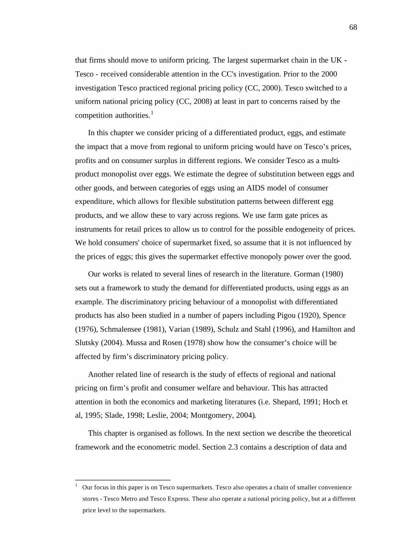
68

that firms should move to uniform pricing. The largest supermarket chain in the UK -

Tesco - received considerable attention in the CC's investigation. Prior to the 2000

investigation Tesco practiced regional pricing policy (CC, 2000). Tesco switched to a

uniform national pricing policy (CC, 2008) at least in part to concerns raised by the

competition authorities.1

In this chapter we consider pricing of a differentiated product, eggs, and estimate

the impact that a move from regional to uniform pricing would have on Tesco’s prices,

profits and on consumer surplus in different regions. We consider Tesco as a multi-

product monopolist over eggs. We estimate the degree of substitution between eggs and

other goods, and between categories of eggs using an AIDS model of consumer

expenditure, which allows for flexible substitution patterns between different egg

products, and we allow these to vary across regions. We use farm gate prices as

instruments for retail prices to allow us to control for the possible endogeneity of prices.

We hold consumers' choice of supermarket fixed, so assume that it is not influenced by

the prices of eggs; this gives the supermarket effective monopoly power over the good.

Our works is related to several lines of research in the literature. Gorman (1980)

sets out a framework to study the demand for differentiated products, using eggs as an

example. The discriminatory pricing behaviour of a monopolist with differentiated

products has also been studied in a number of papers including Pigou (1920), Spence

(1976), Schmalensee (1981), Varian (1989), Schulz and Stahl (1996), and Hamilton and

Slutsky (2004). Mussa and Rosen (1978) show how the consumer’s choice will be

affected by firm’s discriminatory pricing policy.

Another related line of research is the study of effects of regional and national

pricing on firm’s profit and consumer welfare and behaviour. This has attracted

attention in both the economics and marketing literatures (i.e. Shepard, 1991; Hoch et

al, 1995; Slade, 1998; Leslie, 2004; Montgomery, 2004).

This chapter is organised as follows. In the next section we describe the theoretical

framework and the econometric model. Section 2.3 contains a description of data and

1 Our focus in this paper is on Tesco supermarkets. Tesco also operates a chain of smaller convenience

stores - Tesco Metro and Tesco Express. These also operate a national pricing policy, but at a different

price level to the supermarkets.

69

some descriptive analysis. Section 2.4 presents our results and section 2.5 summarises

and concludes.

2.2. Theoretical Model

2.2.1. Firm pricing

We consider a supermarket, Tesco, that operates in r =1,...,R regional markets and

offers j=1,...,J different products (types of eggs) in each market.2 The firm's profits at

period t =1,...,T are given by

( ) ( )∑∑ −−=Πr

rtj

rtjrtjtjrtt CPqmcp , (2.1)

where pjrt is the price of product j in region r at period t,

mcjt is the marginal cost of product j at period t,

qjrt is the quantity of product j sold in region r at period t,

Prt (J × 1) is the vector of prices in region r (jth element is the price of product j)

at period t, and

Crt is the firm’s fixed cost in region r at period t.

We assume that the marginal cost of each type of egg is the same across regions.

Furthermore, regions are considered as separate markets, where the quantity demanded

in each region is a function of only the prices in that region.

National pricing

Tesco currently operates a national pricing policy, which means that pjrt = pjt ; ∀r,j.

We consider the firm to act as a monopolist when pricing eggs. The firm sets j prices to

solve the first-order condition for each of the J products, given by:

( ) 0=∂∂

−+=∂

Π∂ ∑∑∑r k j

krkk

rjr

j pq

mcpqp

for j=1,…,J. (2.2)

The economic interpretation of these equations is that an increase in the price of

product j affects the firm’s profit by (i) decreasing quantity demanded of product j and 2 The number of products offered could differ across regions, but without loss of generality we assume

that all products are offered in all regions.

70

thus decreasing profits, (ii) increasing the profit margin on each unit of product j sold

and thus increasing profits, and (iii) increasing the demand for other products and thus

increasing profits.

Defining ∑=r

jrj qQ equation (2.2) can be rewritten as

( ) 0=∂∂

−+ ∑ ∑k r j

krkkj p

qmcpQ for j=1,…,J, (2.3)

multiplying both sides by ∑k

kk

j

Qp

p and defining the expenditure share on product j

over all regions as ∑=

kkk

jjj Qp

Qps , we can write

( )0=

−+ ∑ ∑

k rkjrkrk

k

kkj s

pmcp

s λω for j = 1, …,J , (2.4)

where j

jrjr Q

q=ω is the quantity share of region r between all regions for product j, and

jkr

krjkjr pq

qp

∂

∂=λ is the jth price elasticity of demand in region r for product k .

Given estimates of kjrλ , and under the assumption that marginal cost does not vary

across regions we can solve these to recover marginal costs for each of the j products.

Regional pricing

If the firm can price discriminate across regions, then the firm sets j×r prices to

solve the first-order condition for each of the j products in each of the r regions, given

by:

( ) 0=∂∂

−+=∂

Π∂ ∑k jr

krkkrjr

jr pq

mcpqp

for j =1,…,J and r =1,…,R. (2.5)

As above, these can be rewritten as:

71

( )0=

−+ ∑

kkjrkr

kr

kkrjr s

pmcp

s λ for j = 1,…,J and r =1,…,R (2.6)

where ( ∑=

kkrkr

jrjrjr qp

qps ). We can solve this set of simultaneous equations for the profit

maximising prices if the firm operated a regional pricing policy (note that this is

possible because we have assumed that marginal cost is constant across regions). In

order to do this we need estimates of kjrλ , and in particular of j

kr

pq

∂∂

. We now turn to

consider how we obtain estimates of these parameters of consumer demand.

2.2.2. Consumer behaviour

We base our model of consumer demand on the Almost Ideal Demand System

(AIDS) (see Gorman, 1980; Deaton and Muellbaeur, 1980; Hausman et al, 1994;

Housman and Leonard, 2007). We estimate a demand system using a three- level

budgeting model, where the top level corresponds to overall demand for eggs, the

middle level represents the choice between the two main categories of eggs, and the

bottom level represent the choice of specific type and size of egg (see figure 2.1 and

table 2.2). The different categories of eggs are partitioned based on their characteristics.

This structure implies that the utility that consumers get from the two categories of

eggs (caged/barn and free-range/organic) are separable, i.e. consumer’s demand for

eggs within one category is not affected by the level of consumption of eggs within the

other category. The substitution between goods in one category depends only on the

prices of goods of that category.

The multi-stage budgeting model implies that at the top level, the consumer decides

how much to spend on eggs as a function of income and a price index for eggs. At the

middle level, the consumer decides how much to allocate to each of two categories as a

function of the price indexes for each category. Having decided on the allocation of

expenditure on each category, at the bottom level the consumer decides how to allocate

this to different eggs in the category as a function the individual prices of all eggs

within that category.

72

Figure 2.1: The three-level budgeting model

We consider the utility of a representative consumer from purchasing eggs as a

separable utility function for the two different categories of eggs, indexed by G =

caged/barn, free-range 3

∑=G

GrtGrtGrtrt EpvU ),( (2.7)

where rtU is the total utility from eggs for region r at period t,

Grtv is the sub-utility from category G eggs for region r at period t,

GrtE is the overall expenditure on category G eggs for region r at period t, and

Grtp is the price vector for category G eggs for region r at period t.

We start at the bottom level and follow Deaton and Muellbauer (1980) by assuming

that consumers' indirect utility within each category (G) takes the form:

( )( )( )GrtG

GrtGrtGrtGrtGrt pb

PEEpv

logloglog

),(−

= , (2.8)

3 Gorman (1959) shows that the functional form consistent with the multi-stage budgeting model is one

of the following (assume only two categories):

U=F[v1 , f(v2 )] or U= v1 + f(v2 )

Where F and f are general continuous functions and f is homogenous of degree one. Gorman rules out the

cases were there are only two categories; Blackorby & Russell (1997) extend Gorman’s results on

multi-stage budgeting to the two group cases.

Small/ Large/ Small/ Mixed/ X-Large/ Medium X-Large Medium Large Organic

Eggs Other Products

Caged/ Free Range/ Barn Organic

Full details of products included in each subcategory is given in table2.2.

73

where ( ) ∑∑∑∈ ∈∈

++=Gk Gj

krtjrtjkrGj

jrtjrrGrt pppaaP loglog21

loglog *0 δ , and

( )( ) ∏∈

=Gj

jrtrGrtGjrppb ββ0log .

In order to find the demand equation, we use Roy’s identity, which tells us that

Grt

Grt

jrt

Grt

jrt

GrtGrtrtjrt

Ev

pv

pE

Epq

∂∂

∂∂

−=∂∂

=),( ,

and find the uncompensated demand equation for each product j. For each product’s the

expenditure share within the category in each time period and in every region is

jrtGk

krtjkrGrt

Grtjrjrjrt p

PE

s εδβα +++= ∑∈

)log()log( ; ∀ j ∈ G &∀ r =1,…,R , (2.9)

where jrts is the expenditure share of subcategory j in category G eggs for region r at

period t,

GrtE is the overall expenditure on category G eggs for region r at period t,

jrtp is the average price of subcategory j for region r at period t,

GrtP is the price index of category G for region r at period t,

2

**kjrjkr

jkr

δδδ

+= ,

jrtε is an idiosyncratic error term, and

jkrjrjr δβα ,, are parameters to be estimated.

As discussed before, Tesco uses a national pricing policy; however, the regional

variations in prices do not arise from differences in the price schedule but instead from

differences in consumer choices. We will discuss this issue in more detail later in

section 2.3.2.

This equation relates the regional expenditure share for product j in a given

category to the total expenditure in that category and prices of all goods in the category.

The jkrδ ’s pick up consumers' willingness to substitute between products. jrα differs

74

across products - all else equal, some products will have higher shares than other

products as a result of differing consumer preferences for products.

The jrβ coefficients allows for non-homotheticity. If jrβ = 0 then the preferences

are homothetic (as category expenditure increases the share spent on each good remains

constant), in which case we can aggregate to the second stage without worrying about

the distribution of income. If jrβ is positive then the share increases with increased

expenditure, and if negative then it decreases. In this case in order to exactly aggregate

we would need to account for the distribution of income across individuals.

The indirect utility defined in (2.8) implies symmetry in consumer substitution

patterns ( kjrjkr δδ = ) which we can test and impose. In addition, the dependent variable

is expenditure shares, so for each period they should add up to one ( 1=∑j

jrts in (2.9)).

Consequently, the coefficients are linearly related:

1=∑j

jrα the constant coefficients in (2.9);

0=∑j

jrβ the category expenditure coefficients in (2.9);

0=∑k

jkrδ the price coefficients in (2.9).

As it is clear from (2.8) to (2.9) that the exact price index is:

∑∑∑ ++=k j

jrtkrtkjrk

krtkrrGrt pppP loglog21

loglog 0 δαα . (2.10)

Using the exact price index involves non- linear estimation, because the coefficients

appear in the price index. Hausman et al (1994) and others suggest using a Laspeyres

price index instead, in order to avoid the non- linear estimation:

jrtGj

jrGrt pP ∑∈

= θ , where ∑∈

=

Gkkrtkrt

jrtj pq

q

00

0θ (2.11)

and t0 is the index for the base period.

We estimate demand at the bottom level using both the exact price index defined in

(2.10) and the Laspeyres approximation defined in (2.11) and show that the results do

not differ significantly. To implement the exact price index, we use the iterated linear

75

least square (ILLE) suggested by Blundell and Robin (1999). In this algorithm, the

exact price index in each step of iteration is calculated using the coefficients calculated

in the previous round. The procedure continues until the coefficients converge. Blundell

and Robin (1999) show that the ILLE estimator is consistent and efficient.

In the middle level, demand for each category is modeled in log- log form:

GrtH

HrtGHrErtGrGrGrt PYQ ξϕβα +++= ∑ )log()log()log( , ∀ r =1,…,R , (2.12)

where GrtQ is the quantity of category G eggs for region r at period t,

ErtY is the total expenditure on eggs for region r at period t ,

GrtP is the price index of category G for region r at period t, the Laspeyers price

index is used for this level.

Grtξ is an idiosyncratic error term, and

GHrGrGr ϕβα ,, are parameters to be estimated.

We impose symmetry in the substitution patterns at this level as well ( rHGGHr ϕϕ = ).

The separability assumption, used in multi-stage budgeting described in equations

(2.9) and (2.11), implies that the expenditure shares within a category depend only on

the category’s expenditure and the prices in that category. Category expenditure

depends on the total expenditure on eggs and the prices for all categories through a price

index. Our model allows a very flexible substitution pattern for different egg products in

the same category. However, the substitution between categories of eggs in different

categories is restricted. A price change for one subcategory of eggs affects the

expenditure share on eggs in another category only through the second level demand

function. Furthermore, this price change affects the demand for all the eggs in the other

category the same way. We will discuss the difference between the cross-price

elasticities for products within the same category and products in two different

categories in more detail in the next section.

At the top level we use a log-log demand function:

rtrtrrtrrrt YQ ζπυγα +++= )log()log()log( , ∀ r =1,…,R , (2.13)

where rtQ is the total number of eggs sold at region r at period t,

76

rtY is the total expenditure on supermarket goods for region r at period t ,

rtπ is the price index of eggs for region r at period t with the general form of

∑=G

GrtGrrt Pρπ ˆ ; we also use a Laspeyres price index.

rtζ is an idiosyncratic error term, and

rrr υγα ,, are parameters to be estimated.

In this paper we use the total expenditure of households on supermarket goods as

proxy for income.

In equation (2.9) the prices of different subcategories of eggs appear on the right

hand side. This raises possible concerns about endogeneity - prices may be correlated

with shocks to demand ( ( )[ ] 0,log ≠jrtrtpE ε , where rtp is the vector of prices in region

r). The correlation between prices and shocks might arise because shocks to expenditure

share for j, which are captured in jrtε , may also affect the way that other goods are

priced. For example, there might be an advertising campaign to promote j which may

also affect the expenditure share of k. If this is the case then OLS estimates of jkrδ will

not be consistent.

The solution is to find instrumental variables ( tz ) that are correlated with rtp

( ( )[ ] 0,log ≠trt zpE ) but are not correlated with jrtε , so that [ ] 0, =jrttzE ε . In other

words, we must be able to exclude tz from equation (2.9), so it has to be the case that it

has no direct effect on jrts and its only effect on jrts is through rtp .

We use data on the cost of different categories of eggs at the farm gate and time

dummies as instruments. We implement this by running a first stage regression relating

price to cost and time dummies, of the form:

jrti

itijrtjrGrt

Grtjrjrjrt c

PE

p ςηηµϕ ++Γ+

+= ∑ )log(log)log( 0 , (2.14)

where jrtp is the average price of subcategory j for region r at period t,

itc is the farm-gate cost of product i at period t ,

77

tΓ is the vector of seasonal and annual time dummies,

GrtE is the overall expenditure on category G eggs for region r at period t,

GrtP is the price index of category G for region r at period t,

rtς is an idiosyncratic error term, and

ijrjrjrjr ηηµϕ ,,, 0 are parameters to be estimated.

The projected prices are then used in place of actual prices to estimate the lower

level demand system.

As mentioned before, for our instruments (the farm-gate prices of eggs and seasonal

and annual time dummies) to be valid, we must believe that the expenditure share for

eggs – and consequently the error terms on (2.9) – are not correlated to these. It seems

reasonable to assume that the expenditure share of different categories of egg does not

vary by farm-gate prices but these costs almost certainly affect price. Our data shows

that the farm-gate prices on average count for about 35% of final prices.

The instruments that may cause concern are the seasonal and annual dummies. It

seems obvious that because of the nature of the poultry industry and storage conditions,

egg prices are seasonally affected. However our data does not show a similar correlation

between the dependent variable in (2.9) and seasonal and annual dummies. Figure 2.2

shows the expenditure shares for our bottom level products in the London region. A

seasonal pattern in these variables is not observed. Furthermore, we also investigated

the effect of exclusion of time dummies from (2.12) and including them in (2.9). The

coefficients for time dummies were not significant. And our results are robust even by

omitting them from our instruments.

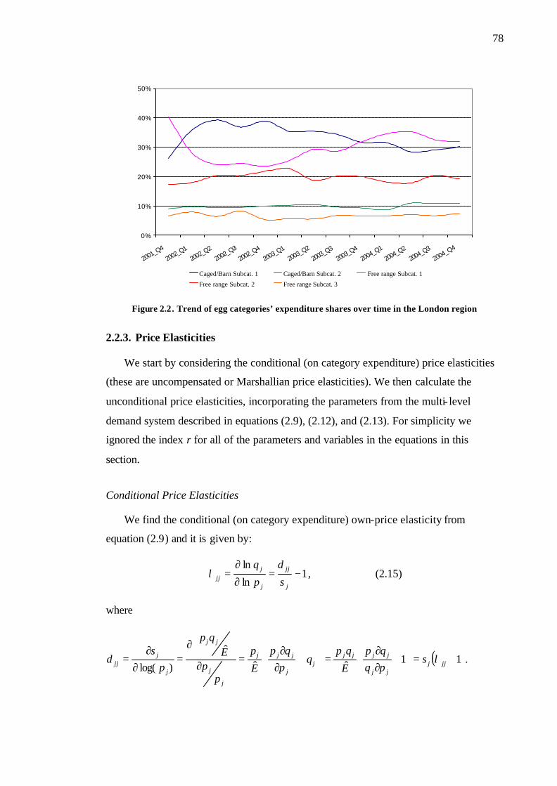
78

0%

10%

20%

30%

40%

50%

2001_Q4

2002_Q

1200

2_Q2

2002_Q3

2002_Q

4200

3_Q1

2003_Q2

2003_Q

3200

3_Q4

2004_Q1

2004_Q

2200

4_Q3

2004_Q4

Caged/Barn Subcat. 1 Caged/Barn Subcat. 2 Free range Subcat. 1

Free range Subcat. 2 Free range Subcat. 3

Figure 2.2. Trend of egg categories’ expenditure shares over time in the London region

2.2.3. Price Elasticities

We start by considering the conditional (on category expenditure) price elasticities

(these are uncompensated or Marshallian price elasticities). We then calculate the

unconditional price elasticities, incorporating the parameters from the multi- level

demand system described in equations (2.9), (2.12), and (2.13). For simplicity we

ignored the index r for all of the parameters and variables in the equations in this

section.

Conditional Price Elasticities

We find the conditional (on category expenditure) own-price elasticity from

equation (2.9) and it is given by:

1ln

ln−=

∂

∂=

j

jj

j

jjj sp

q δλ , (2.15)

where

( )11ˆˆˆ

)log(+=

+

∂∂

=

+

∂∂

=∂

∂

=∂

∂= jjj

jj

jjjjj

j

jjj

j

j

jj

j

jjj s

pqqp

E

qpq

pqp

E

p

pp

Eqp

ps

λδ .

79

Recall that js represents the expenditure share of subcategory j eggs in the category and

E is the overall expenditure of the category.

The conditional (on category expenditure) cross-price elasticities within a category

is given by ( j & k∈ G) (taking derivative of equation (2.9)):

j

jk

k

jjk sp

q δλ =

∂

∂=

ln

ln, (2.16)

where jkjkj

jkjj

k

jjk

k

k

jj

k

jjk s

pqqp

E

qppqp

Ep

pp

Eqp

ps

λδ =∂∂

=∂

∂=

∂

∂

=∂

∂= .ˆ.ˆ

ˆ

)log(.

Unconditional Price Elasticities

The unconditional own-price elasticity is given (for j is a sub-category in the

category G or j ∈ G) by:

( ) ( )1

1ˆ1

ˆ−

+

++++= GG

G

GG

j

jjj

j

jjjj dd

ss

ϕυω

βθ

βδ

λ , (2.17)

where G

jj Q

qd = is the quantity share of subcategory j in category G, and

QQ

d GG = is the quantity share of category G in total number of eggs.

The unconditional cross-price elasticity within a category is given by ( j & k∈ G):

( )

+

++

++= GG

G

GG

k

k

j

jk

j

jkjk dds

ss

ϕυω

βθβδ

λ1ˆ

1ˆ

1 . (2.18)

The unconditional cross-price elasticities between two categories is given by: ( j∈ G

& k∈ H):

( )

++

+= GHH

HG

H

kj

j

jjk

PPp

sϕυω

πβθ

βλ 1ˆˆ1 (2.19)

The detailed calculations are presented in appendix 2.A.

80

Equations (2.18) and (2.19) demonstrate the difference between the cross-price

elasticities for products within a category and between two categories. Equation (2.18)

has two components: the first term has the same form as the conditional cross-price

elasticities (equation (2.16)) which represent the flexible pattern of substitution within a

category, and the second term, which is made up from the middle and top level

coefficients (the income elasticities and the price elasticities from the middle and top

level). However, the cross price-elasticity for products in two different categories

(equation (2.19)) has only one term, which is similar to the second term of (2.18). More

importantly, holding the j index constant, the cross-price elasticity for all k’s products

have almost the same representation.

2.3. Data

We use data from the TNS Worldpanel4 on eggs purchased and brought into the

home by over 20,000 households in the UK over the period December 2001 to

December 2004. The data include the prices paid, quantities purchased, and product

characteristics. Participants record purchases using a hand-held scanner in the house.

Participants are compensated by vouchers which they can spend on durable items. We

consider the variation in demand behaviour across ten regions of the UK - London, the

Midlands, the North East, Yorkshire, Lancashire, the South, Scotland, Anglia, Wales

and the West, and the South West. Eggs are classified by three characteristics: size,

type, and brand.

2.3.1. Characteristics

Size

Four sizes of eggs are sold in the UK: small, medium, large, and extra large. Eggs

can be purchased in single sized or mixed size packages. Small eggs weigh less than 53

grams, medium between 53 and 63 grams, large between 63 and 73 grams, and extra

large eggs more than 73 grams (BEIS, 2009). There are also mixed size packages

which might include eggs from several categories.

Mixed size packages present a difficulty. While consumers are able to compare the

size of eggs easily with other eggs available in the store, we do not observe the size of

4 Described at <http://www.tnsglobal.com/market-research/fmcg-research/consumer-panel>.

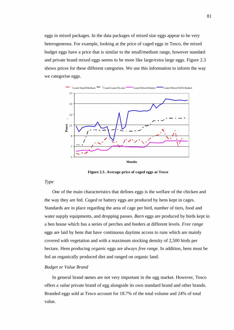
81

eggs in mixed packages. In the data packages of mixed size eggs appear to be very

heterogeneous. For example, looking at the price of caged eggs in Tesco, the mixed

budget eggs have a price that is similar to the small/medium range, however standard

and private brand mixed eggs seems to be more like large/extra large eggs. Figure 2.3

shows prices for these different categories. We use this information to inform the way

we categorise eggs.

5

7

9

11

13

15

17

Months

Penc

e

.

Caged Small/Medium Caged Large/XLarge Caged Mixed Budget Caged Mixed NON-Budget

Figure 2.3. Average price of caged eggs at Tesco

Type

One of the main characteristics that defines eggs is the welfare of the chicken and

the way they are fed. Caged or battery eggs are produced by hens kept in cages.

Standards are in place regarding the area of cage per bird, number of tiers, food and

water supply equipments, and dropping passes. Barn eggs are produced by birds kept in

a hen house which has a series of perches and feeders at different levels. Free range

eggs are laid by hens that have continuous daytime access to runs which are mainly

covered with vegetation and with a maximum stocking density of 2,500 birds per

hectare. Hens producing organic eggs are always free range. In addition, hens must be

fed an organically produced diet and ranged on organic land.

Budget or Value Brand

In general brand names are not very important in the egg market. However, Tesco

offers a value private brand of egg alongside its own standard brand and other brands.

Branded eggs sold at Tesco account for 18.7% of the total volume and 24% of total

value.

82

Cost

The data on cost of each type of egg comes from the British Egg Association. These

data shows the average farm-gate price of each type and size of egg for each quarter.

We use these costs as instruments for prices when we estimate the demand system. The

marginal cost that we calculate includes not only these costs but also distribution and

retail costs.

2.3.2. Descriptive Analysis

We observe over £1m worth of eggs purchased in Tesco in the three years of data

that we use. Table 2.1 shows the volume of eggs purchased by type and size. Of all eggs

sold in Tesco, by far the largest share are caged eggs, followed by free-range, barn and

then organic. By size the largest category is the mixed size packages, followed by large,

medium and extra large. Small represent a negligible share of eggs purchased.

Table 2.1. Distribution of eggs purchased in Tesco, Dec 2001 – Dec 2004

Caged Barn Free-range Organic Total %

Small 65 33 21 0 119 0.0%

Mixed 535385 8124 30582 690 574781 52.3%

Medium 21605 54393 95609 12404 184011 16.7%

Large 25592 63854 100923 13600 203969 18.5%

Extra large 129052 7206 564 0 136822 12.4%

Total 711699 133610 227699 26694 1099702

% 64.7% 12.1% 20.7% 2.4%

Notes: Data are from TNS Worldpanel and include all households observed. The figures are the number

of eggs purchased at Tesco from Dec 2001 to Dec 2004 in TNS data.

Based on the characteristics described above, and an inspection of the average price,

we categorise eggs into five categories, as defined in Table 2.2.

83

Table 2.2. Categories of eggs

Caged and Barn

1) Small / Medium / Mixed (Value) Caged-Small, Caged-Medium, Cage-Mixed-Value, Barn-Small , Barn-

Medium

2) Large / XLarge / Mixed (Other) Caged-Mixed-Standard, Caged-Branded, Caged-Large, Caged-XLarge,

Barn-Mixed, Barn-Large, Barn-XLarge

Free Range and Organic 3) Small/Medium (Value) Free Range-Small, Free Range-Medium-Value, Free Range-Medium-

Standard

4) Mixed/Medium (Branded)/ Large Free Range-Small-Standard, Free Range-Mixed-Standard, Free Range-

Medium-Branded, Free Range-Large

5) Branded/XLarge/Organic Free Range-Mixed-Branded, Free Range-XLarge, Organic all sizes

Table 2.3 shows the regional distribution of purchases of eggs at Tesco. London,

Midlands, and the South regions, which are the most populated areas, have the highest

level of expenditure on eggs, while the North East has the smallest share with just 1.7%

share. Looking at the shares of different categories of eggs purchased in different region

we see that there are significant differences in consumer taste for different categories of

eggs across the regions. For example, while category 1 eggs (Caged and Barn: Small /

Medium / Mixed (Value)) account for 24.8% of expenditure on eggs in the North East,

it accounts for more than twice as much in the South West, where the share is 51.4%.

For category 5 eggs (Free Range Branded/XLarge and Organic) the expenditure shares

vary from 6.1% for the South West to 12.7% for London.

Share

We aggregate the data on egg purchases across households to construct the regional

share of each subcategory of egg. The exact expression is

∑∑∑

∈

=

Gj hjrht

hjrht

jrt e

es ; ∀j∈G (2.20)

where jrts is the expenditure share of subcategory j in category G eggs in region r and

period t, and

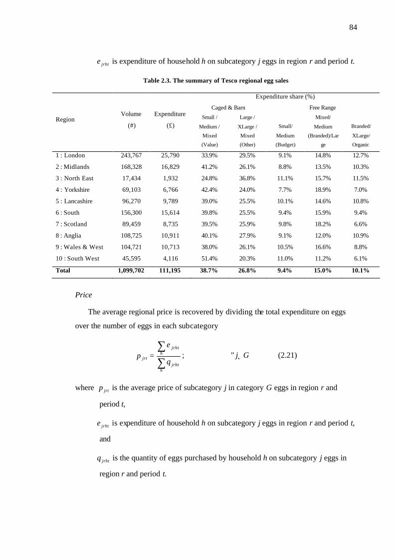
84

jrhte is expenditure of household h on subcategory j eggs in region r and period t.

Table 2.3. The summary of Tesco regional egg sales

Expenditure share (%)

Caged & Barn Free Range

Region Volume

(#)

Expenditure

(£) Small /

Medium /

Mixed

(Value)

Large /

XLarge /

Mixed

(Other)

Small/

Medium

(Budget)

Mixed/

Medium

(Branded)/Lar

ge

Branded/

XLarge/

Organic

1 : London 243,767 25,790 33.9% 29.5% 9.1% 14.8% 12.7%

2 : Midlands 168,328 16,829 41.2% 26.1% 8.8% 13.5% 10.3%

3 : North East 17,434 1,932 24.8% 36.8% 11.1% 15.7% 11.5%

4 : Yorkshire 69,103 6,766 42.4% 24.0% 7.7% 18.9% 7.0%

5 : Lancashire 96,270 9,789 39.0% 25.5% 10.1% 14.6% 10.8%

6 : South 156,300 15,614 39.8% 25.5% 9.4% 15.9% 9.4%

7 : Scotland 89,459 8,735 39.5% 25.9% 9.8% 18.2% 6.6%

8 : Anglia 108,725 10,911 40.1% 27.9% 9.1% 12.0% 10.9%

9 : Wales & West 104,721 10,713 38.0% 26.1% 10.5% 16.6% 8.8%

10 : South West 45,595 4,116 51.4% 20.3% 11.0% 11.2% 6.1%

Total 1,099,702 111,195 38.7% 26.8% 9.4% 15.0% 10.1%

Price

The average regional price is recovered by dividing the total expenditure on eggs

over the number of eggs in each subcategory

∑∑

=

hjrht

hjrht

jrt q

ep ; ∀j∈G (2.21)

where jrtp is the average price of subcategory j in category G eggs in region r and

period t,

jrhte is expenditure of household h on subcategory j eggs in region r and period t,

and

jrhtq is the quantity of eggs purchased by household h on subcategory j eggs in

region r and period t.

85

In 3 cases, for one of the subcategories of the free range eggs we do not observe any

purchases and we exclude these observations from the sample. Two of these cases are

for the North East region and the third one is for the South West.5

Since Tesco used a national pricing policy for the period of the study we expect that

the price of eggs should be the same across regions. However some small regional

variations are observed (see table 2.B1). Variation in prices across regions arises for two

main reasons. First, stores in different regions might put eggs on sale at different times

or with different frequency. Promotions are rarely used for the eggs, so this first source

of variation is not important. Second, each subcategory j includes several different types

and sizes of eggs, which might also be available in different pack sizes (see table 2.2).

We aggregate over these products to measure the average price for each subcategory of

eggs. However, the shares of different products in each subcategory vary over the time.

One reason for this could be changes in the menu of eggs on offer in Tesco nationwide

or in some region. For example, Tesco might decide to replace its own brand of large

caged eggs in packs of 15 with a similar egg in packs of 9. Due to non- linear pricing for

different pack sizes of eggs this would lead to price variation. The lead to a problem of

selection bias: if the price of a certain type of egg changes in a given period, then

consumers might buy this product when it is relatively cheaper. In this case, the average

price observed in our data is different from the average price of products on shelves. We

do not tackle this problem here.

Expenditure

As discussed above, total expenditure of households on supermarket goods is used

as proxy for income. In order to calculate this we aggregate all households’ expenditure

in each region for each period. Table 2.B1 contains summary statistics of all variables

used in the regressions.

5 The issue of missing observations can be tackled using two different approaches. When no purchase is

reported for a subcategory in a region in one period it can be because of one of thes e two reasons:

i) The subcategory was not available in that region in the given period. Based on this assumption the

observation should be excluded.

ii) The product was available but none of the consumer actually preferred that over other products. If

this approach was accepted then the observation should be kept in the sample.

In this case, since the aggregation is performed over purchases of a number of households over a

month, the first approach seems more reasonable.

86

2.4. Results

In this section we present the results of the demand system estimation and discuss

the application of these to analyse the impact on firm profits and consumer welfare of

national and regional pricing policies.

2.4.1. Demand System Estimates

We start with the bottom level results. Table 2.4 presents the estimated coefficients

for equations (2.9) (the bottom level of the demand system) for caged and barn eggs in

the London region. The estimation is performed twice using two different price indexes.

The first estimation is performed using a Laspeyres form approximate price index (as

shown in equation (2.10)). For the second estimation an exact price index, as shown in

equation (2.11), is used. As discussed above, the second estimation has been performed

using the ILLE suggested by Blundell and Robin (1999). The results for the other nine

regions are presented in appendix 2.B in tables 2.B2 and 2.B3. The statistical tests show

that the results from the two estimations have no significant difference.

Table 2.4. London: bottom level results for Caged and Barn using two different price indexes

Price index used: approximate price index exact price index Dep var: share of expenditure on product

Small / Medium / Mixed (Value)

Large / XLarge / Mixed (Other)

Small / Medium / Mixed (Value)

-0.991 − -0.973 Constant (0.305) − (0.327)

0.080 − 0.080 Log (E / P) (0.034) − (0.036)

-0.697 − -0.726 Log (p1) (0.178) − (0.191)

0.358 − 0.473 Log (p2) (0.171) − (0.189)

-2.316 -1.762 Conditional Price Elasticity (0.336) (0.364)

R2 = 0.647; adj-R2 = 0.602; Joint significance; F stat (p-value) = 1.67 (0.192) Homotheticity test; F stat (p-value) = 5.75 (0.022). Notes: Numbers in ( ) are standard errors. Each regression includes 37 observations. (E / P) is the total of expenditure caged and barn eggs in each month over the caged and barn price index, p1 is the average price of Small / Medium / Mixed (Value) for caged and barn eggs in each month, and p2 is the average price of Large / XLarge / Mixed (Other) for caged and barn eggs in each month.

The standard errors reported in the tables have been corrected for the use of a

constructed estimator (the two-stage IV estimation) following Davidson and Mackinnon

(2004). The sign and significance of the coefficients are informative, but the coefficients

87

themselves are not easily interpreted. In the last row we report the conditional (on

category expenditure) own price elasticities (equation 2.15), which are calculated based

on the estimated coefficients. Note that the expenditure elasticity in these tables is the

elasticity of expenditure shares (not quantities) and can be negative or positive. The own

and cross price elasticities are expected to be negative and positive respectively.

The tests for homotheticity of expenditure shares have been performed and the

statistics are reported in table 2.B2 for all regions. The test rejects the null hypothesis of

preference homotheticity for four out of ten regions. However, even for these four

regions the coefficients are ranged from 7.1% to 9.5%, which are relatively small.

The estimation results of the bottom level for free range eggs (equation (2.9)) in the

London region are reported in Table 2.5. Similarly, the estimation is performed twice

using the two different price indexes. The results for all ten regions are included in

appendix 2.B. The statistical tests show no significant difference between the two

models.

Table 2.5. London: bottom level results for Free range

Price index used: Approximate price index exact price index Dep var: share of expenditure on product

Small/ Medium (Budget)

Mixed/ Medium (Branded)/Large

Branded/ XLarge/ Organic

Small/ Medium (Budget)

Mixed/ Medium (Branded)/Large

0.145 -0.292 − 0.101 -0.222 Constant (0.163) (0.192) − (0.255) (0.302)

-0.092 0.112 − -0.072 0.113 Log (E / P) (0.029) (0.028) − (0.045) (0.043)

-1.048 0.093 − -1.035 0.090 Log (p3) (0.159) (0.130) − (0.279) (0.102)

0.093 -0.348 − 0.090 -0.324 log (p4) (0.130) (0.320) − (0.102) (0.536)

0.955 0.255 − 0.945 0.234 log (p5) (0.159) (0.320) − (0.279) (0.536)

-5.174 -1.872 -4.457 Conditional Price Elasticity (0.632) (0.803) (0.941)

R2 = 0.596; adj-R2 = 0.560; Joint significance; F stat (p-value) = 10.5 (0.000). Homotheticity test; F stat (p-value) = 6.06 (0.193) Symmetry test; F stat (p-value) = 1.62 (0.004). Notes: Numbers in ( ) are standard errors. Each regression includes 37 observations. (E / P) is the total expenditure on free-range and organic eggs in each month over the appropriate free-range and organic price index, p3 is the average price of Small / Medium (Budget) for free-range eggs in each month, p4 is the average price of Mixed / Medium (Branded) / Large free-range eggs in each month, and p5 is the average price of Branded / XLarge for free-range and all Organic eggs in each month. Symmetry in cross-price coefficients is imposed.

The results for homotheticity test are included at the bottom of table 2.B4. Only in

three regions the homotheticity assumptions are rejected. In order to perform test of

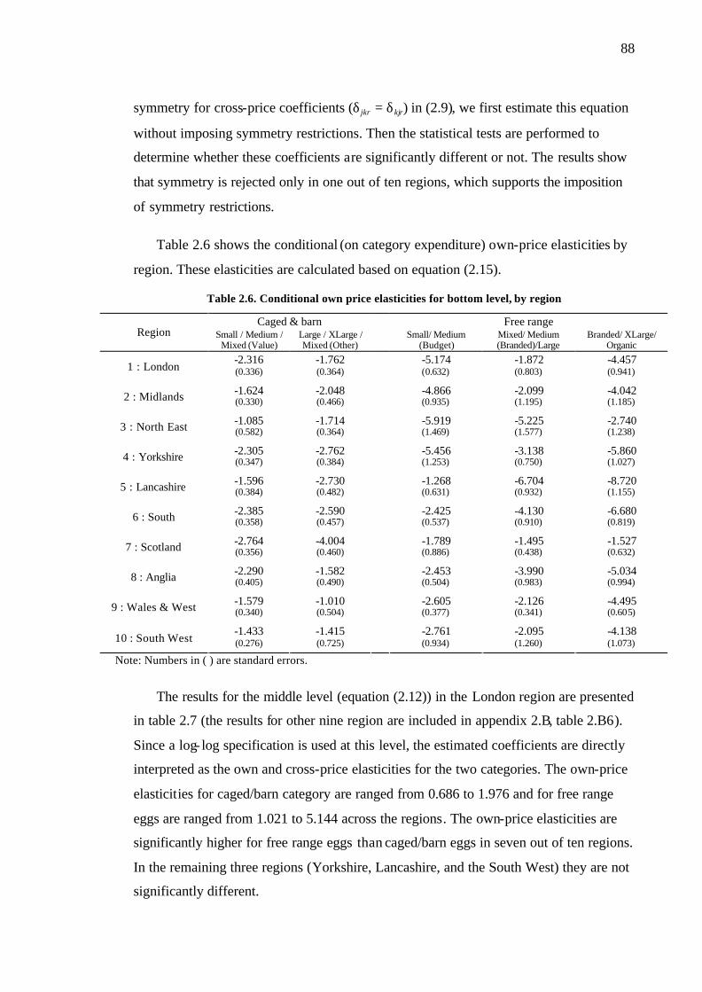
88

symmetry for cross-price coefficients (δ jkr = δkjr) in (2.9), we first estimate this equation

without imposing symmetry restrictions. Then the statistical tests are performed to

determine whether these coefficients are significantly different or not. The results show

that symmetry is rejected only in one out of ten regions, which supports the imposition

of symmetry restrictions.

Table 2.6 shows the conditional (on category expenditure) own-price elasticities by

region. These elasticities are calculated based on equation (2.15).

Table 2.6. Conditional own price elasticities for bottom level, by region

Caged & barn Free range Region Small / Medium /

Mixed (Value) Large / XLarge / Mixed (Other)

Small/ Medium (Budget)

Mixed/ Medium (Branded)/Large

Branded/ XLarge/ Organic

-2.316 -1.762 -5.174 -1.872 -4.457 1 : London (0.336) (0.364) (0.632) (0.803) (0.941)

-1.624 -2.048 -4.866 -2.099 -4.042 2 : Midlands (0.330) (0.466) (0.935) (1.195) (1.185)

-1.085 -1.714 -5.919 -5.225 -2.740 3 : North East (0.582) (0.364) (1.469) (1.577) (1.238)

-2.305 -2.762 -5.456 -3.138 -5.860 4 : Yorkshire (0.347) (0.384) (1.253) (0.750) (1.027)

-1.596 -2.730 -1.268 -6.704 -8.720 5 : Lancashire (0.384) (0.482) (0.631) (0.932) (1.155)

-2.385 -2.590 -2.425 -4.130 -6.680 6 : South (0.358) (0.457) (0.537) (0.910) (0.819)

-2.764 -4.004 -1.789 -1.495 -1.527 7 : Scotland (0.356) (0.460) (0.886) (0.438) (0.632)

-2.290 -1.582 -2.453 -3.990 -5.034 8 : Anglia (0.405) (0.490) (0.504) (0.983) (0.994)

-1.579 -1.010 -2.605 -2.126 -4.495 9 : Wales & West (0.340) (0.504) (0.377) (0.341) (0.605)

-1.433 -1.415 -2.761 -2.095 -4.138 10 : South West (0.276) (0.725) (0.934) (1.260) (1.073)

Note: Numbers in ( ) are standard errors.

The results for the middle level (equation (2.12)) in the London region are presented

in table 2.7 (the results for other nine region are included in appendix 2.B, table 2.B6).

Since a log- log specification is used at this level, the estimated coefficients are directly

interpreted as the own and cross-price elasticities for the two categories. The own-price

elasticities for caged/barn category are ranged from 0.686 to 1.976 and for free range

eggs are ranged from 1.021 to 5.144 across the regions. The own-price elasticities are

significantly higher for free range eggs than caged/barn eggs in seven out of ten regions.

In the remaining three regions (Yorkshire, Lancashire, and the South West) they are not

significantly different.

89

Table 2.7. London: middle level results

Dep var: log of category’s quantity

Caged / Barn Free Range

1.421 1.502 Constant (0.196) (0.206)

1.083 0.906 Log (YE ) (0.030) (0.031)

-1.100 0.172 Log (PC) (0.091) (0.101)

0.172 -1.966 Log (PF) (0.101) (0.254)

R2 = 0.972; adj-R2 = 0.969; Joint significance; F stat (p-value) = 31.04 (0.000) Homogeneity Test; F stat (p-value) = 8.23 (0.001) Symmetry Test; F stat (p_value) = 0.86 (0.357) Notes: Numbers in ( ) are standard errors. Each region’s regression includes 37 observations. YE is the total expenditure on eggs in each region, PC is the price index for caged / Barn eggs in each month, PF is the price for free-range / organic eggs in each month.

The homogeneity test results are included in table 2.B6. The null hypothesis of

homogeneity is rejected in three of the ten regions. The symmetry assumptions for the

cross-price elasticities can not be rejected for any of the ten regions, which supports the

imposition of symmetry restrictions.

Table 2.8 shows the result of the top level regressions (equation (2.12)) for all

regions. Since this is a log- log specification the coefficients are directly interpreted as

the overall income and price elasticities for eggs. All coefficients at this level are

significant. The income elasticities are around one (ranged from 0.973 to 1.257), the

null hypothesis of homogeneity is only rejected in one of ten regions (The South West).

The price elasticities range from 1.353 (Wales) to 3.281 (South West).

90

Table 2.8. Income and price elasticities for the top level

Region Constant Income elas.

log (Y) Price elas.

log(π) R2 Adj R2

Joint sig-nificance

F stat (p-value)

Homo.; F Stats

(p-value)

-3.597 1.055 -3.026 257.9 1.06 1 : London (0.632) (0.054) (0.201) 0.938 0.935 (0.000) (0.310)

-3.362 1.038 -1.928 274.3 0.65 2 : Midlands (0.541) (0.048) (0.168) 0.942 0.938 (0.000) (0.426)

-3.336 1.018 -3.024 60.7 0.04 3 : North East (0.897) (0.096) (0.385) 0.781 0.768 (0.000) (0.843)

-2.509 0.954 -2.320 149.7 0.51 4 : Yorkshire (0.673) (0.064) (0.199) 0.898 0.892 (0.000) (0.480)

-3.320 1.029 -1.650 285.6 0.38 5 : Lancashire (0.505) (0.046) (0.156) 0.943 0.941 (0.000) (0.542)

-2.661 0.973 -2.187 217.7 0.25 6 : South (0.621) (0.055) (0.187) 0.928 0.923 (0.000) (0.620)

-3.091 1.011 -2.441 107.1 0.02 7 : Scotland (0.860) (0.080) (0.243) 0.863 0.855 (0.000) (0.888)

-2.748 0.980 -2.254 234.9 0.16 8 : Anglia (0.536) (0.049) (0.183) 0.933 0.929 (0.000) (0.692)

-3.705 1.064 -1.353 281.9 1.94 9 : Wales & West (0.503) (0.046) (0.172) 0.943 0.940 (0.000) (0.173)

-5.366 1.257 -3.281 109.7 6.66 10 : South West (0.992) (0.100) (0.350) 0.866 0.858 (0.000) (0.014)

Notes: Numbers in ( ) are standard errors; for the F test results numbers in ( ) are p -values. Each regression includes 37 observations on 10 regions. Dependent variable is the log of quantity of eggs bought in region.

Table 2.9 shows the unconditional own-price elasticities, which are calculated using

(2.15). The unconditional own-price elasticities for different categories and different

regions vary between -8.756 and -1.113. These seem high, but note that eggs are highly

substitutable differentiated products. Two well-known papers studying differentiated

product demand systems for food products are Hausman et al (1994) and Nevo (2001).

Hausman et al (1994) uses a similar method to study the beer industry and reports

unconditional own-price elasticities in the region of -6.205 and -3.763. Nevo (2001)

studies the ready-to-eat cereals industry using a discrete choice model. His reported

median own-price elasticities vary between -4.252 and -2.277. Our results are slightly

higher, but comparable with both papers.

91

Table 2.9. Unconditional own-price elasticities

Caged & barn Free range Region Small / Medium /

Mixed (Value) Large / XLarge /Mixed (Other)

Small/ Medium (Budget)

Mixed/ Medium (Branded)/Large

Branded/ XLarge/ Organic

-2.559 -1.905 -5.387 -2.478 -4.808 1 : London (0.336) (0.364) (0.632) (0.804) (0.941)

-1.520 -1.616 -5.324 -2.715 -5.118 2 : Midlands (0.330) (0.466) (0.935) (1.195) (1.186)

-1.236 -2.052 -6.621 -6.637 -3.204 3 : North East (0.582) (0.365) (1.470) (1.578) (1.238)

-2.139 -2.695 -5.199 -2.427 -5.632 4 : Yorkshire (0.348) (0.384) (1.254) (0.750) (1.027)

-1.705 -2.796 -1.301 -6.734 -8.756 5 : Lancashire (0.384) (0.482) (0.631) (0.932) (1.155)

-2.665 -2.716 -2.756 -4.742 -7.109 6 : South (0.358) (0.457) (0.537) (0.910) (0.819)

-2.694 -3.961 -2.109 -1.980 -1.613 7 : Scotland (0.356) (0.460) (0.887) (0.438) (0.632)

-2.705 -1.777 -3.045 -5.234 -7.833 8 : Anglia (0.405) (0.491) (0.504) (0.983) (0.995)

-1.809 -1.113 -2.926 -2.726 -4.807 9 : Wales and West (0.340) (0.504) (0.379) (0.343) (0.606)

-2.512 -1.688 -2.886 -2.375 -4.260 10 : South West (0.276) (0.725) (0.935) (1.261) (1.073)

Note: The table contains unconditional price elasticities based on equation (2.17) and parameters estimated for equation (2.9), (2.12), and (2.13). Numbers in ( ) are standard errors.

As an example to compare the own-price elasticities between two categories, we

consider the most popular subcategory in each of the two categories. These are the first

subcategory (Small / Medium / Mixed (Value)) of caged/barn eggs and the second

subcategory (Mixed/ Medium (Branded)/Large) of free-range eggs. The free-range

subcategory displays significantly higher own-price elasticities than caged and barn

subcategory in five regions (The North East, Lancashire, the South, Anglia, and Wales

and the West). In the remaining five regions the own-price elasticities are not

significantly different for these two subcategories. A similar pattern of higher own-price

elasticities for free range comparing to caged/barn eggs is also observed across other

subcategories.

2.4.2. Marginal Costs

In order to compute the regional profit maximizing profits, we first need to find the

marginal costs for each category of egg. The marginal costs are assumed to be constant

across regions. First the unconditional own and cross-price elasticities for each region

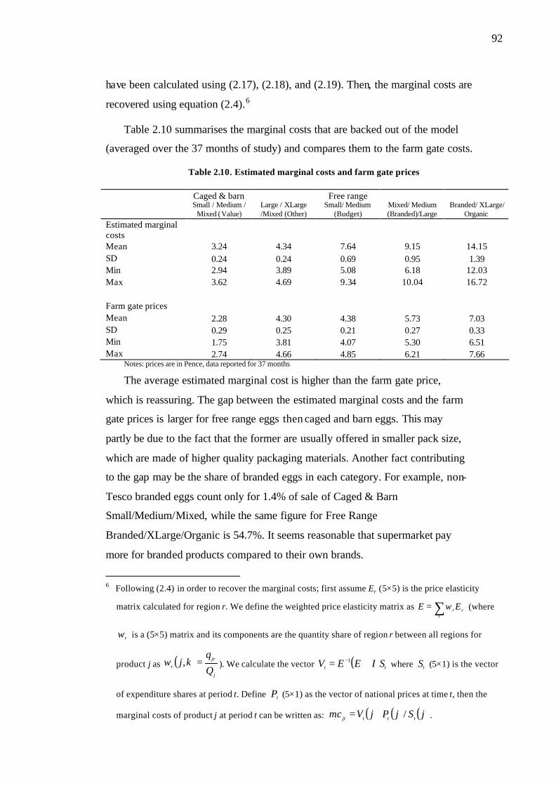
92

have been calculated using (2.17), (2.18), and (2.19). Then, the marginal costs are

recovered using equation (2.4).6

Table 2.10 summarises the marginal costs that are backed out of the model

(averaged over the 37 months of study) and compares them to the farm gate costs.

Table 2.10. Estimated marginal costs and farm gate prices

Caged & barn Free range

Small / Medium /

Mixed (Value) Large / XLarge /Mixed (Other)

Small/ Medium (Budget)

Mixed/ Medium (Branded)/Large

Branded/ XLarge/ Organic

Estimated marginal costs

Mean 3.24 4.34 7.64 9.15 14.15 SD 0.24 0.24 0.69 0.95 1.39 Min 2.94 3.89 5.08 6.18 12.03 Max 3.62 4.69 9.34 10.04 16.72 Farm gate prices Mean 2.28 4.30 4.38 5.73 7.03 SD 0.29 0.25 0.21 0.27 0.33 Min 1.75 3.81 4.07 5.30 6.51 Max 2.74 4.66 4.85 6.21 7.66

Notes: prices are in Pence, data reported for 37 months

The average estimated marginal cost is higher than the farm gate price,

which is reassuring. The gap between the estimated marginal costs and the farm

gate prices is larger for free range eggs then caged and barn eggs. This may

partly be due to the fact that the former are usually offered in smaller pack size,

which are made of higher quality packaging materials. Another fact contributing

to the gap may be the share of branded eggs in each category. For example, non-

Tesco branded eggs count only for 1.4% of sale of Caged & Barn

Small/Medium/Mixed, while the same figure for Free Range

Branded/XLarge/Organic is 54.7%. It seems reasonable that supermarket pay

more for branded products compared to their own brands.

6 Following (2.4) in order to recover the marginal costs; first assume Er (5×5) is the price elasticity

matrix calculated for region r. We define the weighted price elasticity matrix as ∑=r

rr EE ω (where

rω is a (5×5) matrix and its components are the quantity share of region r between all regions for

product j as ( )j

jrr Q

qkj =,ω ). We calculate the vector ( ) tt SIEEV += −1 where tS (5×1) is the vector

of expenditure shares at period t. Define tP (5×1) as the vector of national prices at time t, then the

marginal costs of product j at period t can be written as: ( ) ( ) ( )jSjPjVmc tttjt /⋅= .

93

2.4.3. Profit maximising prices

Using the estimated marginal costs, we turn our attention to equation (2.6), which

defines the firm’s profit maximisation problem. We solve this equation using numerical

methods. Note that as a result of a change in the vector of prices, all quantities

demanded will also change. The expenditure share of each category is therefore a

function of prices. The price elasticities in (2.6) are also a function of prices and

expenditure shares of different categories. In order to find the vector of profit

maximizing prices for each region, we use an iterative procedure to maximise regional

profits in each period. The iterative procedure is:

Step 1) An initial set of prices is assumed (for quick convergence the vector of average

national prices is used).

Step 2) Based on the vector of prices, correspond ing price indexes for the middle and

top level are constructed.

Step 3) Based on the top level price index, the overall demand and expenditure for eggs

are calculated using the coefficients estimated for (2.13).

Step 4) Based on the results of step 3 and the price index for the two middle levels from

step 2, the quantity share of each category is calculated, using the coefficients

estimated for (2.12).

Step 5) Based on the expenditure on each category and the assumed prices, the bottom

level expenditure shares and the quantities are calculated using coefficients

estimated for (2.9).

Step 6) Profit is calculated.

Step 7) Repeat steps 2 to 6 to improve the profit until we find the maximum for the

profit function. 7

Figure 2.4 shows the profit maximizing national and regional prices that we

calculate for caged and barn small/medium eggs (category one). It is clear that the

prices for some of the markets would be lower and some higher under a regional pricing

policy compared to prices under national pricing policy. Consumers in Anglia would

7 While the maximum found using this procedure is not guaranteed to be global; we believe since

national prices are used as the initial values, the results here are the best approximate for regional

profit-maximising prices.

94

face the lowest price, just above marginal cost. This is because Anglia has one of the

highest price elasticities for this category of eggs, compared to other regions. That

means that a marginal increase in price of this category of eggs is likely to decrease the

demand for this category in Anglia more than other regions. The negative effect of this

on profit is higher than the positive effect of the price rise. At the other extreme

consumers in Lancashire, which has a significantly lower price elasticity for this

category of eggs, would face substantially higher regional prices.

National Price

Marginal Cost

0

2

4

6

8

10

12

London

Midlands

North Ea

st

Yorkshi

re

Lancas

hire South

Scotlan

dAngl

ia

Wales & W

est

South W

est

Region

Penc

e .

Figure 2.4. The average national and regional profit maximising prices

for caged and barn small/medium eggs

Table 2.11 shows the average of profit maximizing national and regional prices for

all five subcategories.

Table 2.11. The average national and regional profit maximising prices for all categories

(Unit prices in pence) Caged & barn Free range

Region Small / Medium / Mixed (Value)

Large / XLarge /Mixed (Other)

Small/ Medium (Budget)

Mixed/ Medium (Branded)/Large

Branded/ XLarge/ Organic

1 : London 4.1 9.0 11.8 14.9 19.5 2 : Midlands 8.4 11.9 10.2 11.5 19.0 3 : North East 7.6 6.6 9.7 14.3 19.7 4 : Yorkshire 6.0 10.5 9.8 12.0 25.8 5 : Lancashire 9.4 8.2 17.5 20.7 27.8 6 : South 5.5 10.8 10.4 12.4 18.1 7 : Scotland 6.6 8.7 11.7 13.9 19.2 8 : Anglia 3.7 12.7 12.4 14.0 17.3 9 : Wales and West 9.6 25.9 15.9 17.5 25.9 10 : South West 4.9 6.8 11.9 13.8 21.1 National prices 7.4 11.7 11.8 14.9 21.9

95

2.4.4. Impact on Retailer Profits

What impact would a switch from a national to a regional pricing policy have on the

retailer’s profits? Over the 37 months that we consider moving to a regional pricing

policy would have increased Tesco’s profit on eggs by about 37%. This figure does not

take into the account any extra costs (such as administrative and operational costs)

which might occurs as a result of this policy. Figure 2.5 shows a plot of the estimated

increase in profits in each month as a result of switching to a regional pricing policy.

0%

10%

20%

30%

40%

50%

60%

Dec-0

1Fe

b-02

Apr-0

2Ju

n-02

Aug-

02Oc

t-02

Dec-0

2Fe

b-03

Apr-0

3Ju

n-03

Aug-

03Oc

t-03

Dec-0

3Fe

b-04

Apr-0

4Ju

n-04

Aug-

04Oc

t-04

Dec-0

4

Months

Cha

nge

in P

rofi

t

.

Figure 2.5. The estimated profit gain for Tesco under regional pricing policy

2.4.5. Impact on Consumer Welfare

As mentioned before, the welfare effect of third degree price discrimination is

ambiguous. In order to evaluate the level of utility under each pricing policies we use

equation (2.7). After substituting sub-utilities from (2.8) in (2.7), the total consumer

utility under the national pricing policy is

( )∑ ∏

∑

∈

∈

−

=G

Gjjt

GrtGj

jrtjtNrt jrp

PqpU βˆ

ˆlogˆˆlog, (2.22)

where NrtU is the consumer welfare under national pricing policy in region r and period

t,

96

jtp is the national price of subcategory j in category G eggs in period t,8

jrtq is the regional demand of subcategory j in category G eggs in region r and

period t under national pricing policy,

( ) ∑∑∑∈ ∈∈

+=Gj Gk

ktjtjkrGj

jtjrGrt pppaP ˆlogˆlog21

ˆlogˆlog δ , and

jra , jrβ , and jkrδ s, are coefficients estimated from equation (2.9) and reported in

tables 2.B2 and 2.B4 for all ten regions.

Similarly the total consumer utility under the regional pricing policy is

( )∑ ∏

∑

∈

∈

−

=G

Gjjrt

GrtGj

jrtjrtRrt jp

PqpU β

loglog, (2.23)

where RrtU is the total consumer welfare under regional pricing policy in region r and

period t,

jrtp is the regional price of subcategory j in category G eggs in region r period t

(which calculated in section 2.4.3),

jrtq is the regional demand of subcategory j in category G eggs in region r and

period t under regional pricing policy, and

( ) ∑ ∑∑∈ ∈∈

+=Gj Gk

krtjrtjkrGj

jrtjrGrt pppaP loglog21

loglog δ , and

jra , jrβ , and jkrδ s, are coefficients estimated from equation (2.9) and reported in

tables 2.B2 and 2.B4 for all ten regions.

8 As discussed before, Tesco uses a national pricing policy then we expect jrtjt pp =ˆ for ∀r where the

left hand side is calculated using 2.21. However some regional variations in prices were observed due

to consumer choice. For this part we calculate the national prices using ∑∑∑∑

=

r hjrht

r hjrht

jt q

ep .

97

So the change in consumer welfare in region r and period t, after switching to a

regional pricing policy is Nrt

Rrtrt UUU −=∆ . Table 2.12 shows a summary result of this

change in consumer welfare. Figure 2.6 shows average and range of estimated gain/loss

in consumer welfare across ten regions in case of switching to a regional pricing policy.

As result of the policy change, London and the South West regions are the biggest

winners, and Wales and the west and Lancashire are two biggest losers.

Table 2.12. Summary statistics for the change in consumer welfare

as a result of switching to a regional pricing policy

# Average SD Min Max

Change in

Consumer Welfare 370 4.9% 8.2% -12.9% 27.0%

-15%

-10%

-5%

0%

5%

10%

15%

20%

25%

30%

Lond

on

Midl

ands

North

Eas

t

York

shire

Lanc

ashir

e

South

Scotl

and

Angl

iaW

ales &

West

South

Wes

t

Regions

Cha

nge

in c

onsu

mer

sur

plus

.

Figure 2.6. The average and range of estimated consumer gain/loss across the regions

2.5. Summary and Conclusion

We have estimated a three- level budgeting demand system for Tesco eggs. Using

our estimates of the demand system, we calculated the difference that using a regional

pricing policy would make to Tesco’s profit on eggs and to consumer surplus. Our

estimates suggest that Tesco would substantially increase its profit. The gains to

consumers are modest, with some consumers benefiting, but many losing out.

These results lend some support to the attitude taken by the competition authorities

in their investigations of the supermarket industry.

98

Appendix 2.A

Unconditional Own Price Elasticity

From (2.9) we get

( )jj

j

G

G

jjjj

j

Gj

j

j

pE

E

p

pE

p

sδβδβ +

∂∂

=+∂∂

=∂

∂

)log(log

)log(. (2.A1)

The LHS of (2.A1) is

( )j

G

j

jjjj

G

j

GjjG

j

jjj

jj

G

jj

jj

j

pE

qs

sE

pEqpE

pq

pq

ppE

qp

pp

s∂∂

−+=∂∂−

∂∂

+

=∂

∂

=∂

∂ 2

2 1)log(

λ ;

Substituting this into (2.A1) yields

( )j

G

j

j

G

jjjjjjj p

Eqs

Ep

s∂∂

++=+

2

1 βδλ . (2.A2)

To calculate the last part of (2.A2) we have

( )

∂∂

+=

∂∂

+=∂

∂∂∂

=∂∂

G

GGj

G

GGGj

G

GG

j

G

j

G

PQ

QPQ

PQPQP

pP

pE

loglog

1ˆˆ θθ . (2.A3)

Looking at (2.10)

( ) ( )GG

G

E

GGGG

G

E

E

GGGG

G

EG

G

G

PY

QPY

YP

PY

PQ

ϕβϕβϕβ +∂

∂=+

∂∂

=+∂∂

=∂∂ 1

loglog

loglog

, (2.A4)

And taking derivative of YE with respect to PG

( ) ( ) ( )υωπ

πωπππ

+=

∂∂

+=∂

∂∂∂

=∂

∂1ˆˆ Q

QQ

QPP

YGG

GG

E ; (2.A5)

Substituting (2.A5) into (2.A4) and then (2.A3)

( )

+++=

∂∂

GGGG

GGjj

G QQ

QpE

ϕυωβθ 1ˆ1

1ˆ . (2.A6)

Substituting this into (2.A2)

( ) ( ) jjGGGG

GGjG

jj

j

jjjj Q

QQ

Ep

qs

s δϕυωβθβλ +

+++

+=+ 1ˆ1

1ˆ12

.

99

By defining the quantity share of size j in category G as G

jj Q

qd = and the quantity share of

category G in total number of eggs as Q

Qd G

G = and reordering we get

( ) ( )1

1ˆ1

ˆ−

+

++++= GG

G

GG

j

jjj

j

jjjj dd

ss

ϕυω

βθ

βδ

λ . (2.17)

Unconditional Cross Price Elasticity within a Category:

Differentiating (2.9) with respect to log(pk):

( )jk

k

G

G

kjjk

k

Gj

k

j

pE

Ep

pE

ps

δβδβ +∂∂

=+∂∂

=∂

∂)log(

log)log(

. (2.A7)

The LHS of (2.A7) is

k

G

k

kjjkj

G

k

GjjG

k

jj

kk

G

jj

kk

j

pE

qss

sE

pE

qpEp

qp

ppE

qp

pp

s∂∂

−=∂∂

−∂

∂

=∂

∂

=∂

∂λ2)log(

,

and then substituting into (2.A7) and rearranging we get

jkk

G

G

kj

k

G

k

kjjkj p

EEp

pE

qss

s δβλ +∂∂

=∂∂

− .

Using (2.A6): ( ) jkGGGG

GGkG

kj

k

kjjkj Q

QQ

Ep

q

sss δϕυωβθβλ +

+++

+= 1ˆ

11ˆ ,

Reordering the final expression is

( )

+

++

++= GG

G

GG

k

k

j

jk

j

jkjk dds

ss

ϕυω

βθβδ

λ1ˆ

1ˆ

1 . (2.18)

Unconditional Cross Price Elasticity between two Categories:

The unconditional cross price elasticities between two categories are calculated by taking

the derivative of (2.9) with respect to log(pk), we get ( j∈ G & k∈ H) are

( )k

G

G

kj

k

Gj

k

j

pE

Ep

pE

ps

∂∂

=∂∂

=∂

∂ββ

)log(log

)log(. (2.A8)

100

The LHS of (2.A8) is

k

G

G

kjjkj

G

k

GjjG

k

jj

kk

G

jj

kk

j

pE

Eps

sE

pE

qpEp

qp

ppE

qp

pp

s∂∂

−=∂∂

−∂

∂

=∂

∂

=∂

∂λ2)log(

.

Substituting into (2.A8) gives us

k

G

G

k

j

jjk p

EEp

s ∂∂

+=

βλ 1 . (2.A9)

Calculating the last term of (2.A9) we get

( )

H

G

H

GGj

H

GGk

H

GG

k

H

k

G

PQ

PQP

PQ

PPQP

pP

pE

loglogˆˆ

∂∂

=∂∂

=∂

∂∂∂

=∂∂

θθ . (2.A10)

Looking at (2.11) ( )

GHH

E

E

HGGH

H

EG

H

G

PY

YP

PY

PQ

ϕβϕβ +∂

∂=+

∂∂

=∂∂

loglog

loglog

,

And substituting from (2.A5)

( ) ( ) GHHH

GGHHE

HG

H

G PQ

YP

PQ

ϕυωπ

βϕυωβ ++=++=∂∂

1ˆ1ˆloglog

. (2.A11)

Substituting from (2.A10) and (2.A11) into (2.A9), we finally get:

( )

++

+= GHH

HG

H

kj

j

jjk

PPp

sϕυω

πβθ

βλ 1ˆˆ1 . (2.19)

Appendix 2.B

Table 2.B1. Summary statistics

Unit Mean Std. Dev. Min Max London

log (total expenditure) log(£) 11.795 0.100 11.615 11.965 Log (expenditure on eggs) Log(£) 6.576 0.073 6.392 6.702

log (total quantity) # 8.815 0.142 8.501 9.051 log(π) # 0.013 0.068 -0.089 0.136

Caged / Barn log (quantity) # 8.526 0.152 8.219 8.828

log(PC) # 0.009 0.092 -0.176 0.155 s1 % 52.97% 7.70% 37.54% 64.83%

log (p1) Log(£) -2.586 0.094 -2.729 -2.433 s2 % 47.03% 7.70% 35.17% 62.46%

log (p2) Log(£) -2.146 0.104 -2.409 -1.995 Free Range

log (quantity) # 7.428 0.137 7.097 7.658 log(PF) # 0.018 0.041 -0.034 0.101

s3 % 25.11% 4.21% 14.90% 33.61% log (p3) Log(£) -2.137 0.081 -2.221 -1.924

101

Unit Mean Std. Dev. Min Max s4 % 39.89% 6.19% 24.13% 53.08%

log (p4) log(£) -1.897 0.050 -1.971 -1.807 s5 % 35.01% 8.11% 18.82% 49.88%

log (p5) log(£) -1.518 0.042 -1.598 -1.447 Midlands

log (total expenditure) log(£) 11.383 0.092 11.189 11.563 Log (expenditure on eggs) log(£) 6.148 0.071 5.991 6.308

log (total quantity) # 8.449 0.087 8.251 8.618 log(π) # 0.005 0.069 -0.105 0.119

Caged / Barn log (quantity) # 8.208 0.081 8.033 8.351

log(PC) # -0.004 0.095 -0.194 0.129 s1 % 60.95% 5.84% 44.54% 69.04%

log (p1) log(£) -2.607 0.094 -2.766 -2.472 s2 % 39.05% 5.84% 30.96% 55.46%

log (p2) log(£) -2.153 0.109 -2.428 -2.009 Free Range

log (quantity) # 6.900 0.160 6.458 7.217 log(PF) # 0.018 0.041 -0.030 0.104

s3 % 26.93% 6.00% 13.99% 35.54% log (p3) log(£) -2.143 0.089 -2.248 -1.911

s4 % 41.52% 5.83% 30.38% 53.60% log (p4) log(£) -1.902 0.058 -1.975 -1.776

s5 % 31.55% 6.74% 20.91% 50.46% log (p5) log(£) -1.504 0.069 -1.657 -1.378

North East log (total expenditure) log(£) 9.424 0.201 8.943 9.756

log (expenditure on eggs) log(£) 3.975 0.166 3.637 4.278 log (total quantity) # 6.172 0.171 5.903 6.589

log(π) # 0.028 0.079 -0.145 0.155 Caged / Barn

log (quantity) # 5.828 0.202 5.481 6.368 log(PC) # 0.027 0.105 -0.248 0.172

s1 % 40.39% 11.62% 17.21% 56.99% log (p1) Log(£) -2.594 0.110 -2.871 -2.402

s2 % 59.61% 11.62% 43.01% 82.79% log (p2) Log(£) -2.134 0.122 -2.530 -1.967

Free Range log (quantity) # 4.879 0.350 4.277 5.529

log(PF) # 0.028 0.063 -0.097 0.136 s3 % 29.03% 13.00% 6.53% 58.23%

log (p3) Log(£) -2.161 0.098 -2.300 -1.920 s4 % 42.39% 13.87% 15.36% 80.50%

log (p4) Log(£) -1.901 0.078 -2.139 -1.775 s5 % 30.17% 14.67% 7.01% 62.42%

log (p5) Log(£) -1.507 0.087 -1.793 -1.354 Yorkshire

log (total expenditure) log(£) 10.593 0.109 10.389 10.760 log (expenditure on eggs) log(£) 5.234 0.092 5.004 5.407

log (total quantity) # 7.551 0.145 7.138 7.826 log(π) # 0.021 0.083 -0.120 0.162

Caged / Barn log (quantity) # 7.298 0.147 6.884 7.545

log(PC) # 0.015 0.101 -0.196 0.167 S1 % 63.31% 10.36% 35.11% 82.86%

log (p1) log(£) -2.608 0.089 -2.745 -2.462 S2 % 36.69% 10.36% 17.14% 64.89%

log (p2) log(£) -2.156 0.146 -2.558 -1.954 Free Range

102

Unit Mean Std. Dev. Min Max log (quantity) # 6.043 0.203 5.598 6.417

log(PF) # 0.031 0.062 -0.074 0.185 S3 % 22.58% 8.76% 6.21% 39.53%

log (p3) log(£) -2.162 0.106 -2.288 -1.873 S4 % 56.63% 7.69% 37.38% 71.76%

log (p4) log(£) -1.909 0.067 -2.063 -1.766 S5 % 20.79% 8.01% 5.79% 42.66%

log (p5) log(£) -1.529 0.080 -1.767 -1.419 Lancashire

log (total expenditure) log(£) 10.922 0.093 10.707 11.130 log (expenditure on eggs) log(£) 5.607 0.079 5.417 5.735

log (total quantity) # 7.891 0.096 7.704 8.105 log(π) # 0.016 0.079 -0.130 0.145

Caged / Barn log (quantity) # 7.616 0.116 7.390 7.891

log(PC) # 0.025 0.103 -0.182 0.179 S1 % 60.20% 9.29% 32.50% 76.01%

log (p1) log(£) -2.586 -1.586 -0.586 0.414 S2 % 39.80% 9.29% 23.99% 67.50%

log (p2) log(£) -2.159 0.124 -2.464 -1.979 Free Range

log (quantity) # 6.450 0.147 6.170 6.775 log(PF) # -0.003 0.045 -0.060 0.096

S3 % 28.75% 5.88% 17.29% 41.63% log (p3) log(£) -2.138 0.086 -2.247 -1.945

S4 % 41.16% 10.07% 21.26% 61.50% log (p4) log(£) -1.900 0.065 -2.005 -1.746

S5 % 30.09% 8.68% 13.21% 50.74% log (p5) log(£) -1.521 0.067 -1.716 -1.416

South log (total expenditure) log(£) 11.384 0.074 11.229 11.526

log (expenditure on eggs) log(£) 6.072 0.078 5.942 6.272 log (total quantity) # 8.368 0.135 8.069 8.615

log(π) # 0.021 0.074 -0.112 0.137 Caged / Barn

log (quantity) # 8.102 0.143 7.762 8.394 log(PC) # 0.022 0.095 -0.190 0.153

s1 % 60.86% 8.31% 40.37% 72.15% log (p1) log(£) -2.608 0.093 -2.772 -2.472

s2 % 39.14% 8.31% 27.85% 59.63% log (p2) log(£) -2.158 0.123 -2.502 -1.996

Free Range log (quantity) # 6.905 0.167 6.548 7.321

log(PF) # 0.019 0.046 -0.028 0.112 s3 % 27.03% 4.26% 21.01% 37.46%

log (p3) log(£) -2.143 0.091 -2.234 -1.921 s4 % 45.66% 6.33% 33.55% 64.62%

log (p4) log(£) -1.905 0.051 -1.965 -1.802 s5 % 27.31% 6.95% 13.13% 42.99%

log (p5) log(£) -1.511 0.040 -1.602 -1.452 Scotland

log (total expenditure) log(£) 10.769 0.134 10.523 11.009 log (expenditure on eggs) log(£) 5.489 0.090 5.325 5.698

log (total quantity) # 7.808 0.135 7.505 8.160 log(π) # -0.001 0.083 -0.170 0.126

Caged / Barn log (quantity) # 7.538 0.135 7.204 7.932

log(PC) # 0.001 0.108 -0.266 0.135 s1 % 60.46% 10.85% 32.26% 78.61%

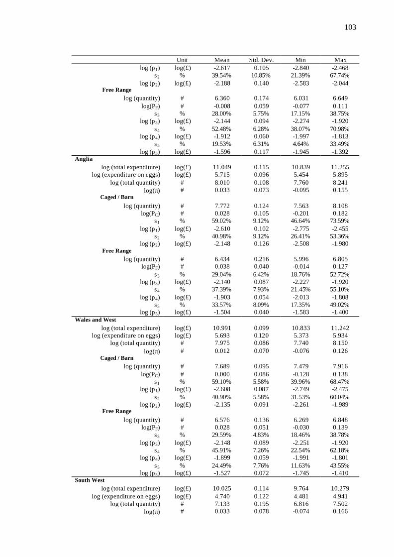
103

Unit Mean Std. Dev. Min Max log (p1) log(£) -2.617 0.105 -2.840 -2.468

s2 % 39.54% 10.85% 21.39% 67.74% log (p2) log(£) -2.188 0.140 -2.583 -2.044

Free Range log (quantity) # 6.360 0.174 6.031 6.649

log(PF) # -0.008 0.059 -0.077 0.111 s3 % 28.00% 5.75% 17.15% 38.75%

log (p3) log(£) -2.144 0.094 -2.274 -1.920 s4 % 52.48% 6.28% 38.07% 70.98%

log (p4) log(£) -1.912 0.060 -1.997 -1.813 s5 % 19.53% 6.31% 4.64% 33.49%

log (p5) log(£) -1.596 0.117 -1.945 -1.392 Anglia

log (total expenditure) log(£) 11.049 0.115 10.839 11.255 log (expenditure on eggs) log(£) 5.715 0.096 5.454 5.895

log (total quantity) # 8.010 0.108 7.760 8.241 log(π) # 0.033 0.073 -0.095 0.155

Caged / Barn log (quantity) # 7.772 0.124 7.563 8.108

log(PC) # 0.028 0.105 -0.201 0.182 s1 % 59.02% 9.12% 46.64% 73.59%

log (p1) log(£) -2.610 0.102 -2.775 -2.455 s2 % 40.98% 9.12% 26.41% 53.36%

log (p2) log(£) -2.148 0.126 -2.508 -1.980 Free Range

log (quantity) # 6.434 0.216 5.996 6.805 log(PF) # 0.038 0.040 -0.014 0.127

s3 % 29.04% 6.42% 18.76% 52.72% log (p3) log(£) -2.140 0.087 -2.227 -1.920

s4 % 37.39% 7.93% 21.45% 55.10% log (p4) log(£) -1.903 0.054 -2.013 -1.808

s5 % 33.57% 8.09% 17.35% 49.02% log (p5) log(£) -1.504 0.040 -1.583 -1.400

Wales and West log (total expenditure) log(£) 10.991 0.099 10.833 11.242

log (expenditure on eggs) log(£) 5.693 0.120 5.373 5.934 log (total quantity) # 7.975 0.086 7.740 8.150

log(π) # 0.012 0.070 -0.076 0.126 Caged / Barn

log (quantity) # 7.689 0.095 7.479 7.916 log(PC) # 0.000 0.086 -0.128 0.138

s1 % 59.10% 5.58% 39.96% 68.47% log (p1) log(£) -2.608 0.087 -2.749 -2.475

s2 % 40.90% 5.58% 31.53% 60.04% log (p2) log(£) -2.135 0.091 -2.261 -1.989

Free Range log (quantity) # 6.576 0.136 6.269 6.848

log(PF) # 0.028 0.051 -0.030 0.139 s3 % 29.59% 4.83% 18.46% 38.78%

log (p3) log(£) -2.148 0.089 -2.251 -1.920 s4 % 45.91% 7.26% 22.54% 62.18%

log (p4) log(£) -1.899 0.059 -1.991 -1.801 s5 % 24.49% 7.76% 11.63% 43.55%

log (p5) log(£) -1.527 0.072 -1.745 -1.410 South West

log (total expenditure) log(£) 10.025 0.114 9.764 10.279 log (expenditure on eggs) log(£) 4.740 0.122 4.481 4.941

log (total quantity) # 7.133 0.195 6.816 7.502 log(π) # 0.033 0.078 -0.074 0.166

104

Unit Mean Std. Dev. Min Max Caged / Barn

log (quantity) # 6.928 0.222 6.581 7.359 log(PC) # 0.058 0.086 -0.064 0.201

s1 % 70.64% 8.71% 41.75% 87.24% log (p1) log(£) -2.642 0.093 -2.783 -2.489

s2 % 29.36% 8.71% 12.76% 58.25% log (p2) log(£) -2.144 0.088 -2.279 -1.960

Free Range log (quantity) # 5.410 0.249 4.771 5.976

log(PF) # -0.039 0.067 -0.151 0.102 s3 % 39.95% 11.06% 16.46% 68.49%

log (p3) log(£) -2.150 0.093 -2.349 -1.920 s4 % 39.25% 11.12% 17.37% 63.19%

log (p4) log(£) -1.912 0.083 -2.067 -1.724 s5 % 21.38% 10.49% 3.47% 46.44%

log (p5) log(£) -1.570 0.114 -1.839 -1.418 Note: π: the Laspeyres price index for eggs; PC: the Laspeyres price index for caged and barn eggs; s1: the expenditure share of Small / Medium / Mixed (Value) sub-category in caged and barn eggs; p1: the price of Small / Medium / Mixed (Value) sub-category of caged and barn eggs; s2: the expenditure share of Large / XLarge / Mixed (Other) sub-category in caged and barn eggs; p2: the price of Large / XLarge / Mixed (Other) sub-category of caged and barn eggs; PF: the Laspeyres price index for free range eggs; s3: the expenditure share of Small / Medium (Budget) sub-category in free range eggs; p3: the price of Small / Medium (Budget) sub-category in free range eggs; s4: the expenditure share of Mixed / Medium (Branded) / Large sub-category in free range eggs; p4: the price of Mixed / Medium (Branded) / Large sub-category in free range eggs; s5: the expenditure share of Branded / XLarge / Organic sub-category in free range eggs; p5: the price of Branded / XLarge / Organic sub-category in free range eggs;

105

Table 2.B2. Bottom level results for Caged and Barn, coefficients for Small / Medium /Mixed (Value)

and conditional own-price elasticities using approximate price index

Dep var: share of expenditure on product

London Midlands North East

Yorkshire Lancashire South Scotland Anglia Wales & West

South West

-0.991 0.092 1.321 -0.578 0.904 -0.270 0.467 -1.027 -0.511 -0.778 Constant (0.305) (0.334) (0.536) (0.426) (0.382) (0.377) (0.375) (0.440) (0.303) (0.319)

0.080 0.071 -0.029 0.094 0.049 0.004 -0.011 0.027 0.073 0.095 Log (E / P) (0.034) (0.034) (0.048) (0.049) (0.041) (0.043) (0.045) (0.048) (0.027) (0.027)

-0.697 -0.380 -0.034 -0.826 -0.359 -0.843 -1.066 -0.761 -0.342 -0.306 Log (p1) (0.178) (0.201) (0.235) (0.220) (0.231) (0.218) (0.215) (0.239) (0.201) (0.195)

0.358 0.409 0.425 0.646 0.689 0.622 1.188 0.239 0.004 0.122 Log (p2) (0.171) (0.182) (0.217) (0.141) (0.192) (0.179) (0.182) (0.201) (0.206) (0.213)

R2 0.647 0.720 0.686 0.619 0.807 0.951 0.946 0.913 0.735 0.701

Adj – R2 0.602 0.685 0.646 0.571 0.783 0.944 0.939 0.902 0.702 0.663

1.67 2.34 1.99 1.48 3.80 17.64 15.93 9.54 2.52 2.13 Joint significance, F stat (p-value) (0.192) (0.091) (0.135) (0.238) (0.019) (0.000) (0.000) (0.000) (0.075) (0.115)

5.75 4.29 0.36 3.71 1.43 0.01 0.06 0.32 7.08 12.39 Homotheticity Test; F stat (p-value) (0.022) (0.046) (0.554) (0.063) (0.241) (0.923) (0.812) (0.574) (0.012) (0.001)

Conditional own-price elasticity

-2.316 -1.624 -1.085 -2.305 -1.596 -2.385 -2.764 -2.290 -1.579 -1.433 Small / Medium / Mixed (Value) (0.336) (0.330) (0.582) (0.347) (0.384) (0.358) (0.356) (0.405) (0.340) (0.276)

-1.762 -2.048 -1.714 -2.762 -2.730 -2.590 -4.004 -1.582 -1.010 -1.415 Large/XLarge / Mixed (Other) (0.364) (0.466) (0.364) (0.384) (0.482) (0.457) (0.460) (0.490) (0.504) (0.725)

Notes: Numbers in ( ) are standard errors; for F-test results numbers in ( ) are p-values. Each region’s regression includes 37 observations. (E / P) is the total of expenditure caged and barn eggs in each month over the appropriate caged and barn price index, p1 is the average price of Small / Medium / Mixed (Value) for caged and barn eggs in each month, and p2 is the average price of Large / XLarge / Mixed (Other) for caged and barn eggs in each month.

106

Table 2.B3. Bottom level results for Caged and Barn, coe fficients for Small / Medium /Mixed (Value) using exact price index

Dep var: share of expenditure on product

London Midlands North East

Yorkshire Lancashire South Scotland Anglia Wales & West

South West

-0.973 0.093 1.328 -0.557 0.901 -0.266 0.471 -1.022 -0.500 -0.757 Constant (0.327) (0.347) (0.568) (0.478) (0.412) (0.410) (0.356) (0.420) (0.287) (0.318)

0.080 0.071 -0.029 0.093 0.049 0.003 -0.012 0.028 0.073 0.095 Log (E / P) (0.036) (0.036) (0.051) (0.055) (0.044) (0.047) (0.043) (0.047) (0.026) (0.027)

-0.726 -0.369 -0.062 -0.836 -0.329 -0.842 -1.078 -0.764 -0.250 -0.329 Log (p1) (0.191) (0.208) (0.244) (0.247) (0.251) (0.242) (0.214) (0.233) (0.196) (0.194)

0.473 0.468 0.426 0.753 0.703 0.625 1.186 0.273 0.012 0.004 Log (p2) (0.189) (0.191) (0.229) (0.166) (0.205) (0.200) (0.173) (0.199) (0.198) (0.216)

Number of iterations 6 5 5 6 5 4 4 5 5 6 Notes: Numbers in ( ) are standard errors. Each region’s regression includes 37 observations. (E / P) is the total of expenditure caged and barn eggs in each month over the appropriate caged and barn price index, p1 is the average price of Small / Medium / Mixed (Value) for caged and barn eggs in each month, and p2 is the average price of Large / XLarge / Mixed (Other) for caged and barn eggs in each month. All simulations started with the initial values of [0.5 0 0 0] for the coefficients; and since the procedure converges quite fast the choice of initial values are not important .

107

Table 2.B4. Bottom level results for Free Range, coefficients for the three sub-categories and conditional own-price elasticities using approximate price index

Dep var: share of expenditure on product

London Midlands North East Yorkshire Lancashire South Scotland Anglia Wales & West

South West

0.145 -0.034 0.013 -0.064 0.454 0.171 0.004 0.733 0.384 0.488 Constant (0.163) (0.140) (0.156) (0.164) (0.188) (0.119) (0.133) (0.119) (0.145) (0.177)

-0.092 -0.051 -0.042 -0.029 0.043 -0.019 0.049 -0.150 -0.075 -0.123 Log (E / P) (0.029) (0.031) (0.063) (0.041) (0.034) (0.026) (0.038) (0.032) (0.029) (0.042)

-1.048 -1.041 -1.428 -1.006 -0.077 -0.385 -0.221 -0.422 -0.475 -0.704 log (p3) (0.159) (0.252) (0.426) (0.283) (0.181) (0.145) (0.248) (0.146) (0.111) (0.373)

0.093 0.269 1.347 0.603 0.051 0.132 0.189 0.093 0.068 0.231 log (p4) (0.130) (0.257) (0.426) (0.303) (0.013) (0.189) (0.229) (0.019) (0.011) (0.389)

0.955 0.772 0.081 0.403 0.026 0.253 0.032 0.329 0.407 0.472

Smal

l / M

ediu

m (B

udge

t)

log (p5) (0.159) (0.221) (0.045) (0.182) (0.181) (0.137) (0.123) (0.146) (0.111) (0.206)

-0.292 0.583 0.478 0.451 -0.187 0.085 0.398 0.267 -0.096 0.274 Constant (0.192) (0.138) (0.234) (0.171) (0.185) (0.130) (0.133) (0.118) (0.143) (0.170)

0.112 -0.036 0.035 0.009 -0.057 -0.022 0.034 -0.062 0.088 0.031 Log (E / P) (0.028) (0.037) (0.065) (0.041) (0.036) (0.026) (0.035) (0.043) (0.029) (0.042)

0.093 0.269 1.347 0.603 0.051 0.132 0.189 0.093 0.068 0.231 log (p3) (0.130) (0.257) (0.426) (0.303) (0.013) (0.189) (0.229) (0.019) (0.011) (0.389)

-0.348 -0.456 -1.791 -1.211 -2.348 -1.429 -0.260 -1.118 -0.517 -0.430 log (p4) (0.320) (0.496) (0.669) (0.425) (0.384) (0.415) (0.230) (0.367) (0.157) (0.495)

0.255 0.187 0.444 0.608 2.297 1.298 0.071 1.025 0.449 0.199

Mix

ed

/ Med

ium

(Bra

nded

) /L

arge

log (p5) (0.320) (0.382) (0.374) (0.229) (0.384) (0.280) (0.024) (0.367) (0.157) (0.237)

R2 0.596 0.590 0.284 0.873 0.400 0.798 0.863 0.253 0.771 0.754 Adj – R2 0.560 0.553 0.220 0.862 0.346 0.780 0.851 0.186 0.750 0.732

10.50 10.22 2.64 48.86 4.73 28.09 44.77 2.41 23.92 21.09 Joint significance, F stat (p-value) (0.000) (0.000) (0.015) (0.000) (0.000) (0.000) (0.000) (0.024) (0.000) (0.000)

1.62 1.96 0.60 2.22 0.75 0.66 0.92 1.59 7.12 0.83 Symmetry Test; F stat (p value) (0.193) (0.129) (0.618) (0.094) (0.526) (0.580) (0.436) (0.200) (0.000) (0.482)

6.06 1.95 0.17 0.18 2.69 0.79 1.89 12.62 3.54 2.95 Homotheticity Test; F stat (p-value) (0.004) (0.150) (0.844) (0.836) (0.075) (0.458) (0.159) (0.000) (0.035) (0.059)

Table continues on the next page

108

Table 2.B4. (continued)

London Midlands North East Yorkshire Lancashire South Scotland Anglia Wales & West

South West

Conditional own-price elasticity -5.174 -4.866 -5.919 -5.456 -1.268 -2.425 -1.789 -2.453 -2.605 -2.761 Small / Medium (Budget) (0.632) (0.935) (1.469) (1.253) (0.631) (0.537) (0.886) (0.504) (0.377) (0.934)

-1.872 -2.099 -5.225 -3.138 -6.704 -4.130 -1.495 -3.990 -2.126 -2.095 Mixed/ Medium (Branded)/Large (0.803) (1.195) (1.577) (0.750) (0.932) (0.910) (0.438) (0.983) (0.341) (1.260)

-4.457 -4.042 -2.740 -5.860 -8.720 -6.680 -1.527 -5.034 -4.495 -4.138 Branded/ XLarge/ Organic (0.941) (1.185) (1.238) (1.027) (1.155) (0.819) (0.632) (0.994) (0.605) (1.073)

Notes: Numbers in ( ) are standard errors; for F-test results numbers in ( ) are p-values. Each region’s regression includes 37 observations (except the North East and

the South West where there are 35 and 36 observations respectively). (E / P) is the total expenditure on free-range and organic eggs in each month over the appropriate

free-range –organic price, index p3 is the average price of Small / Medium (Budget) for free-range eggs in each month, p4 is the average price of Mixed / Medium

(Branded) / Large free-range eggs in each month, and p5 is the average price of Branded / XLarge for free-range and all Organic eggs in each month. (Symmetry

assumption imposed) The critical values of F distribution at 5% significance level are F(8 , 66) = 2.08, F(3 , 64) = 2.75 & F(2 , 66) = 3.14.

109

Table 2.B5. Bottom level results for Free Range, coefficients for the three sub-categories using exact price index

Dep var: share of expenditure on product

London Midlands North East Yorkshire Lancashire South Scotland Anglia Wales & West

South West

0.101 -0.011 0.091 -0.044 0.539 0.162 0.010 0.742 0.468 0.556 Constant (0.255) (0.233) (0.229) (0.299) (0.340) (0.205) (0.228) (0.206) (0.238) (0.296)

-0.072 -0.037 0.038 -0.031 -0.038 -0.020 0.042 -0.119 -0.072 -0.135 Log (E / P) (0.045) (0.057) (0.044) (0.073) (0.061) (0.046) (0.063) (0.056) (0.049) (0.071)

-1.035 -0.955 -1.409 -1.012 0.094 -0.387 -0.269 -0.394 -0.308 -0.701 log (p3) (0.279) (0.401) (0.115) (0.455) (0.345) (0.228) (0.249) (0.275) (0.194) (0.569)

0.090 0.360 1.323 0.627 0.050 0.086 0.195 0.095 0.071 0.296 log (p4) (0.102) (0.402) (0.115) (0.481) (0.000) (0.302) (0.000) (0.000) (0.000) (0.593)

0.945 0.595 0.086 0.385 -0.144 0.300 0.074 0.299 0.237 0.405

Smal

l / M

ediu

m (B

udge

t)

log (p5) (0.279) (0.206) (0.000) (0.370) (0.345) (0.105) (0.249) (0.275) (0.194) (0.596)

-0.222 0.560 0.401 0.452 -0.223 0.107 0.402 0.266 -0.166 0.305 Constant (0.302) (0.231) (0.226) (0.308) (0.335) (0.222) (0.226) (0.205) (0.235) (0.287)

0.113 -0.064 -0.003 0.008 -0.057 -0.022 0.051 -0.089 0.089 0.021 Log (E / P) (0.043) (0.066) (0.041) (0.073) (0.065) (0.046) (0.054) (0.079) (0.048) (0.071)

0.090 0.360 1.323 0.627 0.050 0.086 0.195 0.095 0.071 0.296 log (p3) (0.000) (0.402) (0.115) (0.481) (0.000) (0.302) (0.000) (0.000) (0.000) (0.593)

-0.324 -1.034 -1.784 -1.259 -2.447 -1.316 -0.319 -1.125 -0.679 -0.552 log (p4) (0.536) (0.839) (0.133) (0.673) (0.740) (0.695) (0.241) (0.699) (0.270) (0.764)

0.234 0.674 0.461 0.632 2.397 1.230 0.124 1.030 0.608 0.256

Mix

ed

/ Med

ium

(Bra

nded

) /L

arge

log (p5) (0.536) (0.595) (0.133) (0.594) (0.740) (0.449) (0.241) (0.699) (0.270) (0.840)

Number of Iterations 5 5 5 5 5 4 5 6 5 6 Note: Numbers in ( ) are standard errors.

110

Table 2.B6. Middle level results for all ten regions

Dep var: log of category’s quantity

London Midl ands North East Yorkshire Lancashire South Scotland Anglia Wales & West

South West

1.421 2.149 1.264 1.944 1.616 2.064 1.821 2.057 1.481 1.580 Constant (0.196) (0.233) (0.473) (0.342) (0.339) (0.261) (0.248) (0.293) (0.263) (0.344)

1.083 0.986 1.152 1.029 1.075 0.998 1.042 1.002 1.089 1.158 Log (YE ) (0.030) (0.038) (0.120) (0.066) (0.061) (0.043) (0.046) (0.052) (0.046) (0.073)

-1.100 -0.732 -1.262 -0.595 -1.082 -1.245 -0.686 -1.457 -1.285 -1.976 Log (PC) (0.091) (0.114) (0.395) (0.200) (0.179) (0.127) (0.122) (0.143) (0.215) (0.401)

0.172 0.223 0.900 0.723 0.071 0.212 0.281 0.818 0.264 0.653

Cag

ed &

Bar

n

log (PF) (0.101) (0.151) (0.453) (0.242) (0.234) (0.150) (0.132) (0.171) (0.288) (0.410)

1.502 0.751 2.039 0.824 1.230 0.943 1.334 1.577 1.501 1.662 Constant (0.206) (0.253) (0.511) (0.353) (0.355) (0.278) (0.255) (0.318) (0.264) (0.344)

0.906 1.008 0.730 1.003 0.929 0.987 0.912 0.878 0.902 0.772 Log (YE ) (0.031) (0.041) (0.129) (0.067) (0.064) (0.046) (0.047) (0.055) (0.047) (0.074)

0.172 0.223 0.900 0.723 0.071 0.212 0.281 0.818 0.264 0.653 Log (PC) (0.101) (0.151) (0.453) (0.242) (0.234) (0.150) (0.132) (0.171) (0.288) (0.410)

-1.966 -2.855 -3.460 -0.428 -1.021 -2.208 -1.703 -5.144 -2.222 -1.319

Free

Ran

ge &

O

rgan

ic

log (PF) (0.254) (0.376) (0.835) (0.432) (0.565) (0.351) (0.273) (0.479) (0.498) (0.591)

R2 0.972 0.953 0.725 0.730 0.903 0.956 0.927 0.935 0.593 0.874

Adj – R2 0.969 0.949 0.700 0.706 0.895 0.953 0.920 0.929 0.557 0.863

31.04 18.29 2.38 2.45 8.47 19.91 11.43 12.98 1.32 6.27 Joint significance, F stat (p-value) (0.000) (0.000) (0.031) (0.027) (0.000) (0.000) (0.000) (0.000) (0.255) (0.000)

8.23 0.08 2.77 0.10 1.33 0.04 2.17 2.45 4.05 7.04 Homotheticity Test; F stat (p-value) (0.001) (0.923) (0.070) (0.905) (0.271) (0.961) (0.122) (0.094) (0.022) (0.002)

0.86 0.18 0.01 0.29 1.15 0.78 1.02 0.34 0.02 1.16 Symmetry Test; F stat (p value) (0.357) (0.673) (0.921) (0.592) (0.287) (0.380) (0.316) (0.562) (0.888) (0.285)

Notes: Numbers in ( ) are standard errors; for F-test results numbers in ( ) are p-values. Each region’s regression includes 37 observations. YE is the total on eggs in each region, PC is the price index for caged / barn eggs in each month, PF is the price for free-range / organic eggs in each month.

Chapter 3

The Market for Kidneys in Iran

3.1. Introduction

The most effective treatment for End-Stage Renal Disease (ESRD) is a kidney

transplant (Renal Replacement Therapy: RRT). The only alternative treatment is

dialysis and RRT is the only way for the patient to live without needing dialysis on a

regular basis. Some researchers predict that the number of patient with ESRD will reach

2 million worldwide by 2010 (Nwankwo et al., 2005). In the US, it is predicted that

more than 40% of patients may die while on the waiting list (Matas, 2006). Xue et al.

(2001) predict that more than 95,000 patients will be on the waiting list for a kidney

transplant by 2010; the figure was more than 65,000 in 2007.

There are two sources for a kidney transplant, cadaveric kidneys and kidneys from

the live donors. Cadaveric kidneys can be harvested either from a brain-dead patient

(whose heart is still beating) or cardiacally dead patient; the latter is considered to have

a lower quality. Since a normal person can live on just one kidney, she can decide to

donate one of her kidneys. The incentive to donate a kidney can be altruistic or

obtaining money by selling a kidney. Altruistic kidney donation is mostly a case for

emotionally related donors where the donor donates her kidney to either a relative or a

close friend.

In order to match a kidney from a donor with a potential recipient, their ABO and

RdH blood types as well as tissues should be compatible. The ABO matching should

112

follow the same rules that should be considered for blood transfusion, although some

programs are experimenting with ABO-incompatible transplantation (Gloor & Stegall,

2007). Regarding the tissue matching, a higher proportion of tissues matched between

the donor and recipient will increase the probability of a successful transplantation.

It is well documented that RRT is cost effective treatment as compared to dialysis.

For example the UK national health system (NHS) data reveals that the average cost of

dialysis is £30,800 per year while the cost of kidney transplantation is £17,000

following by a £5,000 annual spend on the drugs. That means over a period of 10 year

(the median graft survival time: the time that transplanted kidney survives in patient’s

body), the average benefit of kidney transplantation, comparing to dialysis, is £241,000

per patient (UK Transplant, 2007).

In order to compare the cost of two alternatives for Iran (all data for 2008); the

annual cost of hemodialysis for a patient is about Rials 47.0m1. The cost of a transplant

operation2 is about Rials 2.4m following by estimated Rials 40.0m annual expenditure

on drugs3. That means from the cost of point of view the transplant is preferred and the

average benefit over the 10 year period is Rials 67.6m. The higher ratio of drug costs

over operation costs in Iran comparing to UK is the result of Iranian system depending

on imported drugs.

It is worth mentioning, the above calculations (both for UK and Iran) are only the

direct benefit of the transplantation by reducing the treatment costs. Three other factors

may also be considered in the cost-benefit analysis i) the opportunity cost of the time,

1 By medical standards, every patients should receive thrice weekly dialysis (equivalent to 156 annual

sessions), but the reported data in Iran shows that the mean annual sessions per patient is just 142. The

tariff for every dialysis session is 92K ("K": medical K; which is determined by the ministry of health

each year and for 2008 is Rials 3600). Then the dialysis cost will be 142×92×3600 ˜ 47.0m.

2 Kidney transplantation tariff is 650K ("K": surgical K; for 2008 is Rials 3700). This value is regardless

of kidney source and method of nephrectomy and includes all expenses from admission to discharge

(both donor and recipient) except some special drugs that sometimes are used for patients with special

conditions or in case of some complications. The costs of initial tests prior to donation or implantation

are not included in this. Then the transplant cost will be 650×3700 ˜ 2.4m.

3 Different immunosuppressive regimens are used for different recipients; therefore, to determine

a unique cost is somehow difficult, however considering the governmental subsidy, which these

drugs receive, Rials 40m is the estimation. Donors receive no drugs routinely; unless complications

happen rarely.

113

patient spends to get dialys is treatment, ii) the improved quality of life for patient after

receiving the transplant, and iii) the risk of death during the surgery for donor. Becker &

Elias (2007) reports that based on several studies, the risk of death during surgery for

donor is between 0.03% and 0.06%. Matas et al (2003) based on the data from the US

transplant centres for period 1993 – 2001 reports the donor’s death rate of around

0.03%.

It is also well known that kidneys from the live sources have a better quality as

compared to the kidneys harvested from cadavers. Table 3.1 contains a summary of the

statistics from US transplants which shows that the kidneys from live donors are more

effective (NKUDIC, 2007). While the 10 year graft survival probability for live kidneys

are 54.7%, the same figure for a cadaveric kidney is only 39.2%.4 One issue that should

be addressed here is the possibility that these data is affected by selection bias. In reality

patients are not randomly matched to kidneys. Terminally ill patients are more likely to

receive a cadaveric kidney which becomes available with lower degree of compatibility.

On the other hand, patients on better conditions can wait a bit longer to receive a more

compatible live donation. Then the cadaveric kidneys may show a lower graft survival

not only because of its own condition but also because of the condition of recipients.

Table 3.1: Survival probability for different treatments

1 year 2 years 5 years 10 years

Patient survival under dialysis 77.7% 62.6% 31.9% 10.0%

Patient survival following cadaveric transplant 94.3% 91.1% 81.2% 59.4%

Patient survival following live-donor transplant 98.2% 95.8% 90.5% 75.6%

Graft survival following cadaveric transplant 89.0% 83.3% 67.4% 39.2%

Graft survival following live-donor transplant 95.2% 91.4% 80.3% 54.7%

Source: NKUDIC (2007)

Harvesting kidneys has been a major concern for health systems all around the

world in the last few decades. In order to increase the kidneys available from cadavers,

two different systems adopted. The most popular one is the opt-in system where people,

who wish to donate their organs after their death, sign up to the scheme. For example it

is estimated that in the UK one in five people (more than 13 million) signed up to the

scheme (Boseley, 2006). This voluntary scheme is run in many countries but usually the

4 Based on the results of a study in 2001 in Iran (not published officially), the graft survival rate in

different intervals for kidney transplants are as follow: 6 months: 90.8%, 12 months: 89.1%, 18

months: 88.2%, 24 months: 87.7%, 30 months: 87.2%, and 36 months: 85.9%.

114

donor’s wish is not enough to guarantee that the donation will take place after the

donor’s death, since in many cases the consent of next of kin is also required, either by

the law or informally. There are campaigns for encouraging organ donations in many

countries. However, the shortfall of the number of organs available through this system

in recent years is an issue; part of the problem is the decreasing number of deaths

among younger people, whose organs are most suitable. For example it is claimed that

one of the reasons behind the drop in the UK cadaveric kidney donation in recent years

(table 3.2) is seat-belt legislation (Boseley, 2006).

The alternative system is the opt-out system which is practised in some European

countries, including Spain and Austria. In this system, the donor’s consent is presumed

and a person needs to opt out the scheme if she does not want to donate her organs after

death. UK also considered switching from opt- in system to this system, where it is

under legal and political consideration (Wintour, 2008)5. One legitimate argument

against this system is that presumed consent means that the state is considered the

owner of the body of deceased person. Some consider this to be a problematic

assumption (Becker & Elias, 2007). Abadie & Gay (2006) develop an economic model

to investigate the effect of presumed consent on the donation rate, their model predicts

that the opt-out system may have a positive or negative effect on the rate of donations

comparing to opt- in system depending on the model assumptions, however, their

empirical analysis for 22 countries over a 10-year period shows after controlling for

other determinants, presumed consent legislation has a positive and significant effect on

organ donation rates.

Another measure to boost the number of donations is an expansive legal definition

of death, such as Spain uses, allowing physicians to declare a patient to be dead at an

earlier stage, when the organs are still in good physical condition. This is controversial

and has been mentioned as the main reason for individuals not wanting to participate in

organ donation schemes. As a result of this procedure, putting extra effort and resources

in procurement process, and the presumed consent system, Spain has one of the highest

rates of cadaveric donations in Europe. (See Table 3.A1 in appendix 3.A) In summary

the high rate of kidney donation in Spain is due to presumed consent policy, enhanced

5 Recently the government committee has recommended against opt-out.

115

infrastructure for donation, expansive legal definition of death, and more road accidents.

However there has been no study to estimate the contribution of each factor.

Table 3.2: The number of live and cadaveric kidney transplantation 1985 - 2006

Iran Spain UK US Year

Live Cada

ver

Total

PMP* Live

Cada

ver

Total

PMP Live

Cada

ver

Total

PMP Live

Cada

ver

Total

PMP

1985 16 0.3

1986 98 1.6

1987 158 2.5

1988 247 4.0

1989 401 6.4

1990 498 7.9 1240 32.2 101 1726 31.9 2094 7322 37.3

1991 571 8.9 16 1355 35.5 88 1608 29.6 2394 7281 38.3

1992 689 10.7 15 1477 38.8 101 1622 30.1 2535 7203 38.5

1993 808 8 12.2 15 1473 38.6 142 1555 29.6 2850 8170 43.5

1994 718 2 11.0 20 1613 42.5 135 1588 30.1 3007 8383 44.1

1995 790 8 11.8 35 1765 46.8 155 1615 30.8 3221 8598 46.3

1996 743 12 11.3 22 1685 44.3 183 1499 29.3 3389 8560 46.7

1997 1078 4 16.3 20 1841 46.9 179 1487 29.1 3597 8577 47.7

1998 1193 2 17.8 19 1976 50.3 252 1330 26.8 4017 8938 50.7

1999 1214 14 18.3 17 2006 50.9 270 1311 26.8 4511 8016 49.5

2000 1389 32 20.5 19 1919 48.7 348 1323 28.3 5311 8087 52.5

2001 1550 70 24.0 31 1893 46.7 358 1333 28.7 5989 8212 49.8

2002 1585 96 24.5 34 1998 48.5 372 1286 28.1 6178 8508 50.9

2003 1474 167 23.9 60 2069 49.8 451 1246 28.7 6464 8665 52.0

2004 1563 207 26.0 61 2125 50.5 463 1367 30.8 6644 9349 54.5

2005 1721 209 27.4 88 2049 48.3 543 1197 29.5 6541 9827 55.3

2006 1615 243 26.4 102 2055 48.3 671 1240 31.7 6434 10659 57.3

2007 1600 311 27.1 137 2074 49.5 804 1207 33.5 6037 10587 54.7

Ave. annual

growth rate

(1996-06)

8.1% 35.1% 16.6% 2.0% 13.9% -1.9% 6.6% 2.2%

Ave. annual

growth rate

(2001-06)

0.8% 28.3% 26.9% 1.7% 13.4% -1.4% 1.4% 5.4%

* PMP: total number of organ donations per million population Source: IRODaT (2009)

There is the argument of conflict of interest in medical teams who should either

declare the death or try to save the badly injured patients. For example in US, in one

case a medical official was accused of trying to end somebody’s life in order to harvest

116

their organs. In another case a doctor said she was under pressure by organ procurement

team, to declare a patient dead sooner than medically advisable (Stein, 2007).6

If the donor is a close relative or emotionally related to the recipient, live donation

is legal in most of the countries around the world. The sale of organs is forbidden in all

countries except in Iran, which has a regulated system for selling kidneys. However,

there is evidence of the abuse of the system in many other countries. Organ trafficking

in India is an example where there are reports of removing the kidneys without donor’s

consent (Patel, 1996)7. Also, there are reports that patients from wealthy countries travel

to poorer countries in order to buy a kidney (Boseley, 2006) which in some cases

removed from donor’s body without their knowledge (Patel, 1996).

In Iran a regulated system for kidney donation with monetary compensation was

introduced in 1980s. Under this regime the donor receives a monetary compensation

from the recipient and enjoys additional monetary and non-monetary bonuses from the

government. The system has been criticised harshly (i.e. Harmon & Delmonico, 2006

and Zargooshi, 2001) as well as receiving some warm support (i.e. Daar, 2006 and

Mahdavi-Mazdeh et al., 2008) both inside Iran and internationally. Ghods & Savaj

(2006) is one of the most recent papers which tries to reason in support of the system by

highlighting the benefits and answering some of the critics. Data show that in 2006

1858 kidney transplantation took place in Iran. 13% and 12% of these transplants were

harvested from cadaveric and emotionally related live sources respectively and the other

75% was from unrelated live donations (Pondrom, 2008).

There has been no discussion on how the system works by economists. While there

were a lot of discussion in medical journals on the Iranian system (for some of the most

recent ones look at Ghods & Savaj (2006), Griffin (2007), and Mahdavi-Mazdeh et al.

(2008)), the lack of publication in economics journals leads to misleading quotes in

other researches. For example Becker & Elias (2007) mention that Iranian government

opposes the cadaveric donation on religious grounds which in not true. On contrary, as

figures in table 3.2 show the Iranian government tries hard to replace the live donation

6 China has also been under pressure for selling the organs of executed individuals (Kram, 2001) where

Chinese transplant centres openly advertise for business from foreigners (Boseley, 2006).

7 Kidney sale was legal in India in 1980s and early 1990s and then became illegal in mid 1990s.

117

with harvesting kidneys from cadavers and the number of other cadaveric organ

donations is also growing fast (Pondrom, 2008).8

Another issue that should be addressed is the compatibility issue. There are two

major considerations regarding the compatibility, blood type and tis sues. Blood type of

the donor and the recipient is needed to have the general compatibility rule for the blood

types (which is being depicted in table 3.3). Even with medical achievements in recent

years to overcome the compatibility issue still incompatibility raises the rejection

probability in transplant. Finding an exact blood type match between recipient and

donor significantly increases the possibility of success. Tissue matching is performed by

testing whether a number of antigens (normally 6 antigens) are matched between

recipient and donor. Higher number of matches in tissues also increases the chance of

success in transplant.

Table 3.3: The compatibility rule for blood and organ donation

Donor

O+ A+ B+ AB+ O- A- B- AB-

O+ ↵ ↵

A+ ↵ ↵ ↵ ↵

B+ ↵ ↵ ↵ ↵

AB+ ↵ ↵ ↵ ↵ ↵ ↵ ↵ ↵

O- ↵

A- ↵ ↵

B- ↵ ↵

Rec

ipie

nt

AB- ↵ ↵ ↵ ↵

In this paper we try to establish clearly how the Iranian regulated system works,

find facts using the data collected from one of procurement centres in Tehran, and

explain the welfare effect of this market on all parties involved. Our finding shows the

average waiting time in Iranian system is around 5 months. This can be considered a

great success compared to average waiting time in other countries.

8 Research grants are also allocated by the Iranian government for research on cloning in order to be

used in organ procurement. There is no significant opposition from religious leaders or other social

pressure groups, but it is very unlikely that these researches lead to a significant breakthrough for

organ procurement in the next decade, not only in Iran but also worldwide (Ghods & Savaj, 2006).

118

Following we start with a brief review on the economics literature on organ

donation in section 3.2. In section 3.3 and 3.4 we demonstrate Iran’s case and present

the data collected from one of the procurement centres. In section 3.5 a theoretical

model will be introduced following by conclusion in section 3.6 which includes our

findings and policy implications.

3.2. Literature Review

Economists have made contribution to the organ donation literature in two fields.

First, the kidney market and issues associated with that. The other is designing a

mechanism to resolve the compatibility issues where donor and recipient are selected.

3.2.1. Kidney Market

Discussion on buying and selling organs or parts of human body (including blood)

can be done on four grounds: medical, moral, legal, and economic grounds. Top

medical experts do not agree on whether the organ market can be implemented or

should be banned.9

From the medical point of view, the evidence as presented in introduction shows

that live donation is efficient and cost effective. Furthermore, if it is safe to be

performed on an emotionally related donor, there should be no medical concern for a

kidney market on the medical grounds. The only point would be to ensure the system

puts the donor’s welfare before the recipient’s; the same rule which should be

considered for an emotionally related pair.

We are not going to discuss moral issues surrounding the kidney sales in full details

in this paper. Roth (2007) explains how the ethical and moral belief of majority of a

society may affect the market as repugnance.

The legal discussions usually concentrate on answering the question of whether an

individual has the right to sell one of her organs or not. For an economist, it might

seems quite a reasonable assumption that one’s body can be considered as their own

property, but defining a property framework for the human body is one of the fresh lines

of research in medical ethics. (i.e. Quigley, 2007)

9 Some of the most recent arguments for and against the idea can be found respectively in Reese et al.

(2006) and Danovitch & Leichtman (2006).

119

The early discussion on the economics of a market for human body parts goes back

to 1970 when Titmuss argued that buying and selling blood has an adverse effect on the

quality of the blood (Titmuss, 1997). Titmuss compares the data from the British system

(where paying for the blood was illegal) with the American system (where blood donors

got paid) and argues that the latter had a lower quality of denoted blood. Titmuss points

out that a significant fraction of the American blood came from individuals with

hepatitis and other diseases that could not be screened out, and the blood given under

the British system tended to be healthier. Titmuss also argued that monetary

compensation for donating blood might reduce the supply of blood donors. This

hypothesis often referred to as crowding out effect. Titmuss predicts that people will

give blood mainly for altruism and introducing money compensation into the system is

going to diminish their incentives for blood donation.

Becker (2006) argues that even if Titmuss was right about the qua lity of the blood,

the American system provides more blood per capita than British system. This means

that the crowding out effect is not present. However, the quality of blood is not a major

problem now, since the modern screening methods can guarantee the blood is not

contaminated. In case of kidneys, one can argue that medical developments can

determine the well-being of the donor and recipient. On the other hand, since kidney

transplant is a more complicated and costly procedure comparing to blood transfusion,

the initial test for the donor in order to assess the quality of the kidney, as well as the

donor’s safety and welfare, would be more justifiable.

Mellström & Johannesson (2008) ran a field experiment on the blood transfusion

system in Sweden to examine whether the crowding out effect can be determined. They

designed three treatments. In the first one, subjects are given the opportunity to become

blood donors without any compensation. In the second treatment subjects receive

monetary compensation (SEK 50 ˜ $7), and in the last one subjects can choose to

receive the payment or donating it to charity. Their experiment shows evidence for the

crowding out effect only on some part of population (women) which will be eliminated

if the monetary payment made to charity rather than the individual.

Cohen (1989), Epstein (1993), and Kaserman & Barnett (2002) discuss the

monetary compensation for cadaveric organ donations but Becker & Elias (2007) are

the first to calculate a price for live kidneys. They calculate a price of a kidney (and a

liver) based on three monetary compensations i) compensation for the risk of death as a

120

result of donation, ii) compensation for the time lost during recovery, and iii)

compensation for the risk of reduced quality of life. They suggest a price of $15,200 for

a kidney. They also point out that if the market for cadaveric kidneys established

alongside the live kidney market, most kidneys will come from cadavers and live kidney

prices works as a benchmark for the market equilibrium price for cadaveric kidneys.10

3.2.2. Kidney Exchange Mechanisms

One of the main restrictions for emotionally related organ donations is the

compatibility issue, where the donor’s kidney cannot be transplanted for their intended

recipient. But it might be compatible with another patient who also has a non-

compatible donor.

Roth et al. (2004) introduce a kidney exchange mechanism which efficiently and

incentive compatibly, can increase the number of transplants within existing constraints.

Their model resembles some of the housing problems studied in the mechanism design

literature for indivisible goods (i.e. Shapley & Scarf, 1974 and Abdulkadiroglu &

Sönmez, 1999). Modified versions of their model, in order to limit the number of

simultaneous operations needed, with constraint on the maximum number of donor-

patient pairs to two or three, has been developed in later papers (Roth et al., 2005b;

Roth et al., 2007; and Saidman et al., 2006). Roth et al. (2005a) provides evidence from

the experiment of opening a kidney clearinghouse in New England, US.

In an exceptional case a 6 way exchange performed in the US on April 2008 (BBC,

2008). However, because of practical issues (the exchange operations should be done

simultaneously and most possibly at the same hospital) as well as incentive issues

(where medical teams should work together and it is most likely doctors in small

hospitals should refer almost all of their patients to other centres) the exchange

mechanism cannot provide enough kidneys to overcome the shortage.

10 If Becker & Elias (2007) suggestion for paying for cadaveric kidneys and livers is going to be

practiced; one issue, which should be addressed, is its effect on health costs of other transplantations

from cadaveric sources, like hearts and corneas. Currently no payment has been made for harvesting

these organs which under the new system it seems plausible to assume they should be priced as well.

One argument can be since the demand for these organs are not as high as kidney and liver the

equilibrium price will not be significantly high and the altruistic donation may be enough to cover the

demand. However, this issue can be subject of a separate research.

121

3.3. Iran’s Case

3.3.1. Background

The 1979 revolution in Iran was followed in 1980 by an eight year war with Iraq.

Dialysis equipment was scarce because of economic sanctions and lack of funds for

imports (Nobakht & Ghahramani, 2006). As a result of these events, nephrologists were

encouraged to perform kidney transplant s. At the beginning, the process relied on few

cadaveric kidneys available, along with emotionally related donors. But the large

number of patients on the waiting list forced the authorities to establish a regulated

market for living unrelated donations. The efforts of charities, established and managed

by dialysis patients and their close relatives, helped to develop the market. Table 3.2

shows a clear picture of the development of kidney transplantation in Iran. It is notable

that over a period of 10 year (1996-2006) the rate of cadaveric and live donation

increased by 35.1% and 8.1% annually. Cadaveric transplants accounted for 1.6% of

total number of transplantation in 1996, this figure reached 13.1% in 2006.

3.3.2. Institutions

There are several bodies involved in kidney procurement for patients in need of a

kidney transplant in Iran:

1) Kidney Foundation of Iran (or Dialysis and Transplant Patients Association

(DATPA)) is a charity founded by some of kidney patients and their relatives about 20

years ago. The foundation is a non-governmental organisation and helps kidney patients

with their problems. With 138 branches around the country, they help kidney patients

with medical, financial, and other problems. In about 10 centres they have kidney

donation offices. Their main and busiest office is located in Tehran. The foundation also

has official support of the Charity Foundation for Special Diseases.

2) Office of the Governor of Tehran (Ostan-dari) has also an office for kidney

donation which has limited activities comparing to the Kidney Foundation. There are

similar offices in some other provinces located in the governors’ headquarters.

3) Management Centre for Transplantation and Special Diseases which is part of

the Ministry of Health and Medical Education and is responsible for cadaver transplant.

This centre has different waiting lists for patients in need of various organs for

transplantation and is the main (and only) centre involved in procurement of organs

122

from cadavers. The centre’s database ran nationally. When cadaveric organs of a

deceased patient become available, the centre allocates the organs (including kidneys) to

transplant centres around the country considering different factors including distance

and waiting time.

In summer 2007, there were around 1000 patients on their waiting list for kidney

transplant. As it can be seen in table 3.2, in 2005 from 1854 kidney donation, 243 cases

were from cadavers. That means around 13% of the kidneys come from cadaver

sources. Religious and traditional views are a major barrier for cadaveric donations,

however, in recent years the numbers of cadaveric of transplants is increasing. A

scheme of donor registry (opt- in system) is designed and some individuals, especially

young educated Iranians, have shown interest in signing to the scheme. But in practice

the relatives of the dead person have veto power and they can overrule the original

decision made by the person herself, as it is the case in many other count ries with the

opt-in system (Abadie & Gay, 2006).

3.3.3. How Does Unrelated Kidney Donation in Iran Work?11

The Kidney Foundation keeps waiting lists for kidney patients with different blood

types in each of its procurement offices. There are eight different lists for different

blood types (see table 3.3). A kidney patient, who wishes to be added to the waiting list,

needs to present a letter from his doctor. Since the foundation does not run any initial

tests on patients, some patients may enter the list when they are not medically ready for

a transplant. This may cause unintended delays in the matching process. A patient

should be at a certain stage of the kidney failure disease to be considered ready for the

transplant; and his general physical conditions (for example strength or minimum

weight) also play a significant part in increasing the probability of success in operation.

A patient is given priority in the waiting list, if he either is medically in an emergency

situation (as assessed by his doctor) or is a disabled soldier12.

There is no centralised waiting list and each centre has its own waiting list. Patients

are asked by foundation to book in their nearest centre but some patients enter several

waiting lists (including the cadaveric waiting list) in order to minimise their waiting

11 This section is based on our interviews with the foundation staff, other sources and some published

papers.

12 Mostly injured in the eight year war with Iraq (1980-88).

123

time. However, the centres coordinate with each other in case of imbalances (especially

for emergency cases) of demand and supply for kidneys with a particular blood type.

Medical staff including the members of the transplantation team have no role in

identifying potential donors. When a donor (aged between 22 and 35)13 turns up to

donate her kidney, she needs to provide certain documents; including a formal consent

from either her spouse or her father (in case of un-married donors)14. After the initial

official paperwork, she will be referred to a clinic for the initial medical tests. The

foundation office in Tehran has its own clinic which is used in order to offer medical

support for kidney patients. Using this clinic speeds up the initial process. These tests

determine whether the potential donor has any sort of kidney problem as well as a

simple blood test and whether her kidney has two renal arteries15. If the transplantation

team suspected any possible harm to the donor either now or for the future, the donation

will be cancelled. The costs of these tests, which are not high, have to be paid by the

donor herself. Since the cost of these tests (estimated around Rials 50k) is not

significantly high comparing to the monetary compensation, it does not seem to have an

adverse effect on donors’ decision.

After the donor passes the initial tests, the administrators contact the first patient in

the same waiting list as the donor’s blood type. In this stage the staff also has in their

mind to match the physical build of the donor and the patient or at least make sure that

they are not extremely different. This also raises the issue of finding a suitable match for

child patients which is difficult. Matches cross different blood types are rare and they

13 The reason for the age cap is considered to be a higher chance of the graft survival. Some researches

on live donation do not support that the lower the age of the donor has a significant relationship with

higher graft survival period. For example El-Agroudy et al (2003) shows that the average age for the

live donor when kidney survived for more than 15 years was 30 ± 8.6 while for the graft survival rate

less than 15 years was 35 ± 10.7. Another research (El-Husseini et al., 2006) reports for a 10 year graft

surviving period, these figures as 37.1 ± 9.4 and 36.2 ± 8.5 respectively. However, it always will be the

case that any operation (like being a kidney donor) is considered with a substantial risk after an age

threshold.

14 In Absence of next of kin, to make sure the donor is aware of her action and its consequences, she will

be referred to a chartered psychologist at the coroner’s office for a psychic test.

15 Most patients are not happy to have a kidney transplant from this type, since it reduces the chance of

successful transplant. However, some researches show no difference regarding this (Makiyama et al.,

2003).

124

try to match the blood type of the donor and the recipient. Since having the same blood

type is going to increase the possibility of a successful transplant (comparing to

alternative transplants between compatible blood types), usually the doctors also advise

their patients to wait for an exact match.

If the patient who is on the top of the waiting list at the moment is not ready for the

transplant at that moment, the next patient will be called, and so on, until a ready patient

will be found. Then a meeting between the two parties is arranged (they are provided

with a private area within the foundation building if they want to reach a private

agreement) and they will be sent for tissue tests. If the tissue test gives the favourable

result16, a contract between the patient and the donor will be signed and they will be

provided with a list of the transplant centres and doctors who perform surgery. When

the patient and the donor are referred to transplant centre, a cheque from the patient will

be kept at the centre to be paid to the donor after the transplant takes place. The guide

price has been 25m Rials (≈ $2660) until March 2007 for 3 years and at this time17 it has

been raised to 30m Rials (≈ $3190).18 This decision has been made because the

foundation was worried of a decreasing trend in number of donors. In some cases, the

recipient will agree to make an additional payment to the donor outside the system; it is

not certain how common this practice is, but according to the foundation staff the

amount of this payment is not usually big and is thought to be about 5m to 10m Rials (≈

$530 to $1060). The recipient also pays for the cost of tests, two operations, after

surgery cares, and other associated costs (like accommodation and travel costs if the

patient travels from another city). Insurance companies cover the medical costs of the

transplant and the operations are also performed free of charge in state-owned hospitals.

In addition, the government pays a monetary gift to the donor for appreciation of

her altruism (currently, 10m Rials), as well as automatic provision of one year free

health insurance19, and the opportunity to attend the annual appreciation event dedicated

16 According to administrators of the foundation less than 10% of the tests have a positive cross-match

which effectively rules out transplantation. It should be noted that the more tissue matching factor

leads to a higher probability of success.

17 The Iranian new year starts at 20 March. The adjustment happened at the start on new year.

18 The exchange rate for 20 Feb 2008: $1 ≡ Rials 9410; £1 ≡ Rials 18400.

19 Nobakht & Ghahramani (2006) claim that the donors are provided with a free life -long insurance

which is in contrary with our findings, after interviews with the foundation staff.

125

to donors20. The Charity Foundation for Special Diseases also provides the donors with

a free annual medical test and high level of support, in case that the donor develops

kidney problems in the future, regardless of whether this is due to the transplant or not.

Emotionally related donors also enjoy these monetary and non-monetary bonuses as

well as exemption of paying hospital costs, and it gives them a good incentive to

register in the foundation offices.

The minimum monthly legal wage for 2007 was Rials 1,830k (later raised to 2,200k

for 2008). The minimum payment of Rials 45m is around 2 years of minimum wage.21

The minimum current payment (45m Rials) by using PPP exchange rate22 is

equivalent to $14,000 which is interestingly close to Becker & Elias (2007) suggestion

for the market value of a kidney at $15,200 for the US. In 1980s when the sale of kidney

was legal in India, donors were paid $1,603. After making this illegal in 1990s the

average payment dropped to $975 (Goyal et al., 2002). Based on this paper and other

researches, Becker & Elias (2007) estimate that the equivalent cost of a kidney in Indian

market to US dollar in 2005 is in region of $17,078 to $17,665. However, they even

report a price of around 50,000 Rupees in 1980s which with their calculations will be

equivalent to $81,510 in the US market for 2005.

The government decision to ease the process by legislation and monetary and non-

monetary bonuses seems reasonable. The social negative effect of losing ESRD patients

who are usually at working age and most possibly parents of underage children is quite

significant. This decision is also justifiable on economic grounds, from the government

and insurers point of view. A patient, who is going under constant dialysis, is going to

spend a lot of time out of the job. Adding up to this opportunity cost, the financial

burden for the dialysis on the patient, his family, social services, and the government

20 This event is an event to celebrate the altruism of family of cadaver organ donors as well as living

kidney donors. Among the guests are also all the organ recipients. The events gather a very good

publicity in media; usually to emphasis the importance of cadaveric donors.

21 This figure is the minimum wage which is well below the minimum cost of living. The Iranian Central

Bank reports the monthly average cost of living for a family of four to be Rials 8.7m for Tehran and

Rials 6.64m for other urban areas. This makes the minimum compensation equivalent to 5.2 to 6.7

months of average cost of living in urban areas.

22 For PPP exchange rate an average of indexes suggested by IMF, and World Bank is used.

126

and considering a higher probability of death while in the waiting list, having no option

for live transplant; shows the high alternative cost for the society.

Advertising for kidney donors is banned. However, some patients manage to find

donors from other informal channels in order to avoid the waiting list. The foundation

handle these cases with due care and such cases need to be reviewed by the foundation

managing director. However, since the bonus payment appreciation and other

protections by the government are in place for donors, then any donation that takes

place is registered in one of the foundation offices around the country. This includes

most of donations from family members which recipient and donor do not involve in

any financial transactions.

In order to prevent international kidney trade, the donor and recipient are required

to have the same nationality. That means an Afghan patient, who is referred to the

foundation, should wait until an Afghan donor with appropriate characteristics turns up.

This is to avoid transplant tourism. Transplant tourism seems to be a problem in India

(Patel, 1996). Another issue can be Iranian nationals residing abroad and travel to Iran

to buy a kidney, which is allowed under current legislation. 23

Although the insurance companies will not cover the donor’s compensation, poor

recipients can get help in order to provide the cost from different charities. The

foundation staff also have an informal list of generous volunteers, who are eager to help

poor patients financially.

By the foundation’s procedure to keep 8 different waiting lists, if one assumes that

the blood type distribution is the same between patients and potential donors then the

waiting time would be fairly similar for all waiting lists, furthermore there will be no

significant social benefit in matching between blood groups.

23 Official statistics show that around 1m refugees live in Iran mostly with Afghan and Iraqi origins

(Some claim the actual figure is far more and in some stages over the past 20 years has even reached to

around 3 million). Ghods and Savaj (2006) refer to a study on nationality of transplant recipients and

kidney donors. From 1881 kidney transplants, 19 (1%) recipients were refugees, and 11 (0.6%) were

other foreign nationals who received kidneys from living-related donors or from living-unrelated

donors of the same nationality. Of 1881 recipients, 18 (0.9%) also were Iranian immigrants (residing

abroad for years) who came and received kidneys from Iranian paid donors. The scale of transplant

tourism is very small in Iran.

127

One of the concerns about employing the Iranian system would be the possible

welfare effect on the minorities because of the different pattern of the blood type

distribution in their blood types. Table 3.A2 shows the blood type distribution of blood

donors in different provinces. This data shows only the geographical distribution of the

blood donors and usually is biased in favour O and negative blood types, since usually

blood transfusion centres encourage these types of blood types to be donated more.

However, looking at these data one line of the fresh research in Iranian system would be

to investigate the proportion of different ethnic and race minorities in the pool of kidney

donors and recipients. Walter et al. (1991) summarises the result of few other researches

in Iranian ethnic variability of blood type frequencies based on ABO alleles (Their

finding can be found on table 3.A3). Since their divisions in Iran population is neither

consistent (have some geographical division and some ethnic minorities) nor inclusive

(do not show a clear picture of the whole country) their findings can be addressed as

another source of concern for this issue. They specially point out that Assyrian,

Armenians, Zoroastrians, Jews, Turkmans, and Arabs, all religious and ethnic

minorities, show a significant different pattern of ABO frequencies, however, they

report a significantly lower percentage of O alleles for all of these minority groups than

the Iranian average.

There are two major papers which address the donors’ satisfaction issue. Zargooshi

(2001) surveys 300 of kidney donors. They donated between 6 to 132 months ago. He

finds that the majority of donors either did not receive or did not attend follow-up visits.

Many of them regretted their original decision. On contrary Malakoutian et al (2007)

report a 91% satisfaction between living kidney donors. However, the latter survey is

asked the donors at the point of discharge from hospital.

3.4. Data

Our data contains 598 transplantations recorded in Tehran office of the Kidney

Foundation between April 2006 and December 2008. In fact, this is the number of

patients who withdrew from the waiting list with a kidney transplant in these 21 months.

Of these, 549 were live kidney donations of which 539 were traded kidney and 10

emotionally related donations. The remaining 49 transplantations took place with a

cadaveric donation. In theory the waiting lists for live and cadaveric kidneys run

independently; and the coverage of our data from cadaveric transplant is not complete.

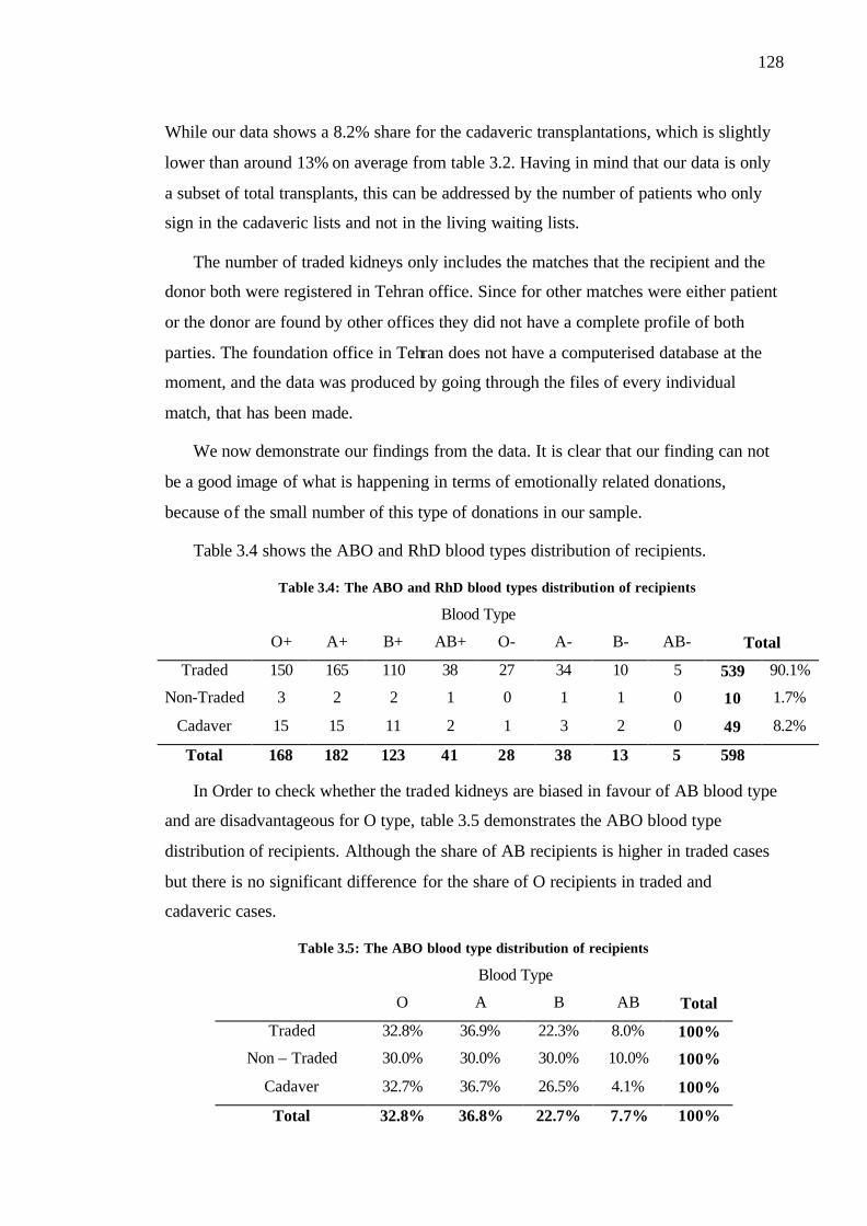
128

While our data shows a 8.2% share for the cadaveric transplantations, which is slightly

lower than around 13% on average from table 3.2. Having in mind that our data is only

a subset of total transplants, this can be addressed by the number of patients who only

sign in the cadaveric lists and not in the living waiting lists.

The number of traded kidneys only includes the matches that the recipient and the

donor both were registered in Tehran office. Since for other matches were either patient

or the donor are found by other offices they did not have a complete profile of both

parties. The foundation office in Tehran does not have a computerised database at the

moment, and the data was produced by going through the files of every individual

match, that has been made.

We now demonstrate our findings from the data. It is clear that our finding can not

be a good image of what is happening in terms of emotionally related donations,

because of the small number of this type of donations in our sample.

Table 3.4 shows the ABO and RhD blood types distribution of recipients.

Table 3.4: The ABO and RhD blood types distribution of recipients

Blood Type

O+ A+ B+ AB+ O- A- B- AB- Total

Traded 150 165 110 38 27 34 10 5 539 90.1%

Non-Traded 3 2 2 1 0 1 1 0 10 1.7%

Cadaver 15 15 11 2 1 3 2 0 49 8.2%

Total 168 182 123 41 28 38 13 5 598

In Order to check whether the traded kidneys are biased in favour of AB blood type

and are disadvantageous for O type, table 3.5 demonstrates the ABO blood type

distribution of recipients. Although the share of AB recipients is higher in traded cases

but there is no significant difference for the share of O recipients in traded and

cadaveric cases.

Table 3.5: The ABO blood type distribution of recipients

Blood Type

O A B AB Total

Traded 32.8% 36.9% 22.3% 8.0% 100%

Non – Traded 30.0% 30.0% 30.0% 10.0% 100%

Cadaver 32.7% 36.7% 26.5% 4.1% 100%

Total 32.8% 36.8% 22.7% 7.7% 100%

129

Another concern could be discriminating against women in receiving kidneys.

Traditionally in Iran, men are referred as breadwinner of the family. Although the sex

pattern of labour force has been changed, but it is still biased towards a higher

proportion of male workers. Since in this view, the economic value of a man is

considered to be higher, one consequence in our argument can be a higher likelihood for

a male patient receiving a kidney from traded sector. Table 3.6 shows the number and

percentage of male and female recipients. The figures do not support any negative effect

on female patients in our data.

Table 3.6: The sex of recipients of each type of kidney

Male Female Total

350 189 539 Traded

(64.9%) (35.1%) (100.0%)

5 5 10 Non-Traded

(50.0%) (50.0%) (100.0%)

33 16 49 Cadaver

(67.3%) (32.7%) (100.0%)

Total 388 210 598

On the other hand the donors are mostly men (Table 3.7). This can be because of

the two facts. Firstly, the ages between 22 and 35; when the donation is accepted; is the

fertility age; and women are less likely to be considered as potential donors. Secondly,

as we mentioned before since men are supposed as the main breadwinner of the family,

it is more likely that they sell their kidneys in order to overcome financial difficulties.

Female donors count for around 18% of traded kidneys in our data; it is in contrary with

the Indian case where 71% of the sold kidneys were from female donors (Goyal et al.

2002).24

Table 3.7: The sex of donors of each type of kidney

Male Female Total

Traded 446 93 539

Non-Traded 4 6 10

Total 450 99 549

Table 3.8 demonstrates the age distribution of recipients and donors of traded

kidneys. It shows that 10.9% of the recipients are under the age of 20. Finding kidneys

24 Indian data needs to be treated very carefully, since the kidney sale is illegal. However, the difference

between two figures is quite significant.

130

for child patients is one of their main problems. The kidneys for these children should

be small in size, and usually women donors are the best to match for these patients. The

high number of transplants needed for relatively young patients (42.9% under the age of

40 and 65.3% under the age of 50), shows the economic and social value of these

transplants. Although the foundation’s policy is to limit the donors’ age to 35, 10.4% of

the donors are older than 35.

The joint blood type distribution of recipients and donors can be seen at table 3.9.

On average 94.8% of kidneys are matched to an exact blood type. In total 28 cases out

of 539 are matches between different blood types. The reason behind this can be

emergency cases, matches found by patients themselves out of the formal system, and

especial cases (like children recipients when the size of kidney plays an important rule).

Table 3.8: Age distribution of recipients and donors

Age Recipients Donors

5 – 9 12 2.2%

10 – 14 19 3.5%

15 – 19 28 5.2%

20 – 24 36 6.7% 148 27.5%

25 – 29 50 9.3% 216 40.1%

30 – 34 42 7.8% 119 22.1%

35 – 39 44 8.2% 51 9.5%

40 – 44 59 10.9% 5 0.9%

45 – 49 62 11.5%

50 – 54 58 10.8%

55 – 59 65 12.1%

60 – 64 40 7.4%

65 – 69 16 3.0%

70 – 74 7 1.3%

75 – 79 1 0.2%

Total 539 100.0% 539 100.0%

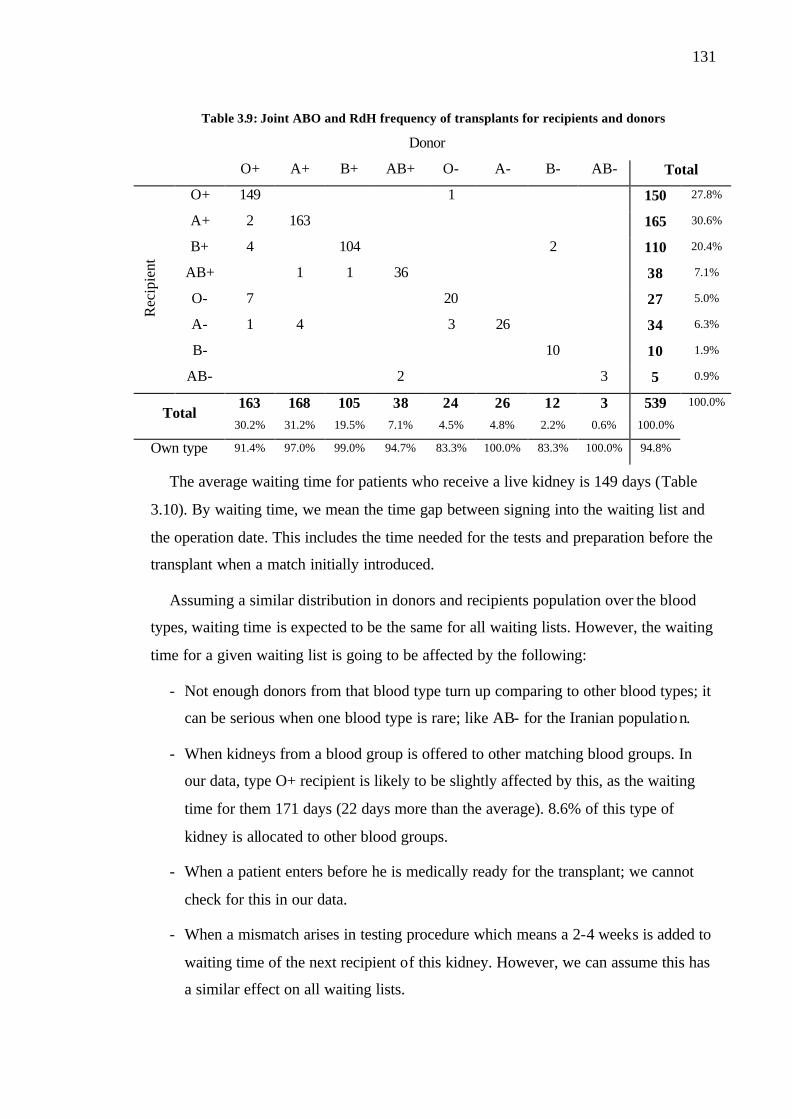
131

Table 3.9: Joint ABO and RdH frequency of transplants for recipients and donors

Donor O+ A+ B+ AB+ O- A- B- AB- Total

O+ 149 1 150 27.8%

A+ 2 163 165 30.6%

B+ 4 104 2 110 20.4%

AB+ 1 1 36 38 7.1%

O- 7 20 27 5.0%

A- 1 4 3 26 34 6.3%

B- 10 10 1.9%

Rec

ipie

nt

AB- 2 3 5 0.9%

163 168 105 38 24 26 12 3 539 100.0% Total

30.2% 31.2% 19.5% 7.1% 4.5% 4.8% 2.2% 0.6% 100.0%

Own type 91.4% 97.0% 99.0% 94.7% 83.3% 100.0% 83.3% 100.0% 94.8%

The average waiting time for patients who receive a live kidney is 149 days (Table

3.10). By waiting time, we mean the time gap between signing into the waiting list and

the operation date. This includes the time needed for the tests and preparation before the

transplant when a match initially introduced.

Assuming a similar distribution in donors and recipients population over the blood

types, waiting time is expected to be the same for all waiting lists. However, the waiting

time for a given waiting list is going to be affected by the following:

- Not enough donors from that blood type turn up comparing to other blood types; it

can be serious when one blood type is rare; like AB- for the Iranian population.

- When kidneys from a blood group is offered to other matching blood groups. In

our data, type O+ recipient is likely to be slightly affected by this, as the waiting

time for them 171 days (22 days more than the average). 8.6% of this type of

kidney is allocated to other blood groups.

- When a patient enters before he is medically ready for the transplant; we cannot

check for this in our data.

- When a mismatch arises in testing procedure which means a 2-4 weeks is added to

waiting time of the next recipient of this kidney. However, we can assume this has

a similar effect on all waiting lists.

132

- As mentioned before the guideline price increased by 20% on March 2007. But

our data shows no significant change in the waiting time or the number of

donation. It could because of two reasons; firstly this increase has almost no

significant effect in real term because of inflation25. In fact considering the

inflation the official level of payment has been decreased over the 3 years when it

has been capped prior to March 2007. Secondly the price that actually paid in each

case can be different from this benchmark by two parties’ negotiation process and

it can also make that increase less significant.

Table 3.10: Average waiting time for recipients based on the blood type of both parties

Donor

O+ A+ B+ AB+ O- A- B- AB- Average

O+ 169 461 171

A+ 110 138 137

B+ 85 138 214 138

AB+ 104 32 128 125

O- 163 117 129

A- 92 205 249 177 184

B- 124 124

Rec

ipie

nt

AB- 218 144 174

Average 163 165 139 137 133 148 177 139 144

Considering all of the mentioned factors, having a waiting list of around 5 months

in Iranian system comparing to more than 3 years for some other countries seems a

significant achievement. One question that may arise (also by looking at tables 3.2 and

3.A1) is that the overall rate of kidney transplantation in Iran is not particularly higher

than its European and north American counterparts, then why the Iranian waiting lists is

much shorter. The fact is that the rate of ESRD patients in Iranian population is lower as

well. One of the main reasons behind this can be the Iranian population structure, in

2006 (latest census) 60.5% are below 30 and 86.1% are below 50 years old (SCI, 2007).

It is estimated that in 2005, 1505 per million population (pmp) in North America, 585

pmp in Europe, and 370 pmp in Iran suffered from ESRD. (Grassmann et al., 2005)

Following, we list the possible policy considerations:

25 The reported rate inflation for 2006-07 is 18.4%.

133

- Since the donors might be subject to exploitation because of their social status; it

needs to be guaranteed that they make an informed decision and are aware of all

risks attached to their decision.

- After donation networks needs to be strengthened in order to make sure the donors

receive the best support possible.

- Considering the Iranian population structure, it is expected that the demand might

rise for kidneys in coming years and decades. Then, more efforts need to be put

on other sources of kidneys. Cadaveric kidneys can be utilised more effectively.

Unlike some developed countries, Iran faces no social barrier in new frontiers in

medical research, e.g. cloning. Investing in this area may help to eliminate the

demand for live donation in the future.

- A national waiting list can reduce the waiting time as well as improving pre- and

post- surgery support for both donors and recipients.

3.5. Model

Suppose we have a continuum population with the total mass normalised to one. Let

there be two blood types X and Y, with shares of α and 1-α of the population

respectively. The probability of a person being in need of a kidney is r regardless of her

blood type, however a shock of δ is considered for demand of type X kidneys; which

can be positive or negative.26 We assume that the demand for each type of kidney can

be written as:

( ) ( )XDX Pgrq αδ+= 1 and ( ) ( )Y

DY Pgrq α−= 1 (3.1)

where 0 < α < 1 ;

0 ≤ r << 1 ; −1 ≤ δ << 1/r −1 ;

0<′g ; and ( ) 10 =g

26 The shock is only considered for type X kidneys. From the overall welfare point of view analysis of a

positive (negative) shock to demand for type Y kidney is equivalent to a negative (positive) shock to

type X. However, the effect in welfare on each market can be different which is not important for our

discussion here.

134

Assume that type X kidney cannot be dona ted to type Y, but type Y kidneys can be

donated to type X recipients. Suppose the income distribution is independent of blood

types, so the supply has the same functional form for both types. Then the supplies can

be written as:

( )XSX Pfq α= and ( ) ( )Y

SY Pfq α−= 1 (3.2)

where 0>′f

In the absence of the shock ( 0=δ ), the equilibrium price for both markets is the

same ( ) ( )PgrPf ˆˆ = .

We assume that the regulator observes all the parameters of the market except the

shock. Furthermore the regulator is able to allocate the kidneys efficiently. That means

even if the market price is less than market clearing price, patients with the highest

priority (highest willingness to pay) will receive kidney and the maximum feasible

consumer surplus will be achieved. The regulator sets a uniform price for both markets.

This price is equal to the market clearing price in the absence of the shock. The

regulator is now faced with the problem whether to allow trade between the markets or

not.

Negative shock ( 0<δ ):

At the price set by the regulator ( P ) there is now excess supply of type X kidneys.

Since type Y cannot receive type X kidneys, the equilibrium in the Y market remains

unchanged. In the X market the quantity reduces. Figure 3.1 shows this situation where

D and D’ are the original demand and demand in presence of a negative shock,

respectively. Allowing the intra-trade is making no difference on the outcome and social

welfare in this case. However, since the regulatory price is now higher than the market-

clearing price, total welfare is reduced. The highlighted area in figure 3.1 shows this

loss.

135

Figure 3.1: Demand and supply in X type markets

in presence of a negative shock to demand for X

Positive shock ( 0>δ ):

At the price set by the regulator P there is now excess demand for type X kidneys.

If intra-trade between the two markets is allowed, some of type Y kidneys will be sold in

type X market. In order to achieve the maximum welfare in this case some of the Y

kidneys should be allocated to X patients. Y kidneys should be allocated to X recipients

until the marginal willingness became the same in both markets (dashed red line in

figure 3.2). Figure 3.2 compares the gain and loss in consumer surplus in X and Y

market. The graph to the left demonstrates type X market where D and D’ representing

demand in absence and presence of a shock respectively. The right graph presents the

case for type Y. The two arrows show the welfare- improving shift in supply after a

positive shock to demand for X. The two marked areas shows the gain and loss resulted

by intra-trade.

Allowing the intra-trade has no effect on the supplier surplus. The consumer surplus

gained by type X patients overweighs the loss in type Y patients’ consumer surplus.

Overall patients’ welfare improves as a result of intra-trade in case of a positive shock

to demand for X.

S

D’

D

Pric

e X Type

Quantity

P

136

Figure 3.2: Demand and supply in two blood-type markets

in presence of a positive shock to demand for X

It is worth mentioning even if the regulator sets a price different from the

equilibrium price; still this welfare analysis is true. In presence of a positive shock to

demand for X, Whatever the price set by the government, allowing intra-trade reduces

the consumer surplus for type Y and consumer surplus for type X increases. The latter

always dominates and the outcome is a higher social welfare resulted by intra-trade.

3.6. Summary and Conclusion

In this paper, we investigate how the Iranian kidney market works. Our focus was

not on the moral and ethical issues surrounding the discussions. The effect of the Iranian

system on reducing the waiting time for patients is significant, which based on our data

it is around 5 months. One should be careful in advising to ban the sale at all. The

alternative solution practiced in other developing countries, e.g. black market for

organs, might have dramatic consequences. This may result lower standards on medical

conditions, as well as leaving the donors who can be vulnerable without any official

support.

We showed that allowing intra-trade between different blood types although has a

negative effect on the welfare of some patients, but is going to improve the social

welfare.

S

S

D’

D

D

Pric

e

Pric

e X Type Y Type

Quantity

Quantity

P

137

Appendix 3.A

Table 3.A1: Number of kidney transplants per million population for some countries in 2006

PMP (per million people)

Country Live Cad. Total Country Live Cad. Total

Cyprus 54.3 11.4 65.7 Poland 0.5 23.5 24.0

US 21.6 35.7 57.3 Slovenia 0.0 24.0 24.0

Austria 7.0 41.5 48.5 Argentina 4.9 16.7 21.6

Spain 2.3 46.0 48.3 Israel 7.7 12.4 20.1

Norway 17.1 28.1 45.2 New Zealand 11.3 8.4 19.7

Belgium 4.0 40.6 44.6 South Korea 14.1 4.9 19.0

Uruguay 2.5 41.8 44.3 Greece 5.7 13.1 18.8

France 4.0 38.0 42.0 Puerto Rico 3.5 15.3 18.8

Malta 10.0 30.0 40.0 Mexico 13.7 4.6 18.3

Netherland 17.1 22.1 39.2 Lebanon 16.0 2.0 18.0

Finland 0.6 38.3 38.9 Brazil 9.6 8.2 17.8

Portugal 3.8 33.2 37.0 Lithuania 1.8 15.9 17.7

Canada 15.0 21.5 36.5 Colombia 1.9 13.4 15.3

Czech Rep. 3.2 33.1 36.3 Pakistan 15.1 0.0 15.1

Switzerland 15.7 19.9 35.6 Estonia 0.7 13.4 14.1

Ireland 1.0 32.4 33.4 Turkey 10.1 4.0 14.1

Denmark 10.7 22.1 32.8 Brunei 13.4 0.0 13.4

Latvia 0.0 32.6 32.6 Cuba 0.7 9.9 10.6

Germany 6.3 25.8 32.1 Romania 7.9 1.9 9.8

UK 11.2 20.6 31.8 Hong Kong 1.9 7.6 9.5

Hungry 1.3 29.6 30.9 Qatar 2.6 4.0 6.6

Jordan 30.5 0.0 30.5 Guatemala 6.0 0.4 6.4

Australia 13.3 16.0 29.3 Trinidad & Tobago 6.2 0.0 6.2

Italy 1.5 27.6 29.1 South Africa 2.1 3.0 5.1

Iran 23.0 3.4 26.4 Bulgaria 0.3 4.6 4.9

Iceland 26.0 0.0 26.0 Ukraine 1.4 1.1 2.5

Slovak Rep. 5.4 20.4 25.8 Malaysia 0.9 1.0 1.9

Saudi Arabia 9.3 16.4 25.7 Gerogia 1.8 0.0 1.8

Croatia 4.5 20.3 24.8 Moldova 0.6 0.0 0.6

Source: IRODaT (2008)

138

Table 3.A2: The ABO and RdH blood type distribution of Iran provinces *

ABO RdH

O A B AB + -

Azarbayejan Gharbi 37.4% 20.9% 32.9% 8.8% 90.2% 9.8% 1.62%

Azarbayejan Sharghi 37.3% 20.9% 33.9% 7.9% 88.6% 11.4% 7.08%

Booshehr 27.2% 27.2% 40.1% 5.4% 92.5% 7.5% 0.10%

Chahar Mahal & Bakhtiari 32.1% 19.5% 43.9% 4.5% 88.8% 11.2% 0.32%

Fars 28.8% 24.9% 39.0% 7.2% 90.4% 9.6% 2.02%

Gilan 30.5% 22.1% 41.0% 6.4% 89.2% 10.8% 4.90%

Hamedan 32.9% 23.7% 35.8% 7.6% 91.0% 9.0% 3.85%

Hormozgan 19.9% 28.1% 46.2% 5.8% 91.8% 8.2% 0.06%

Ilam 37.3% 23.6% 32.3% 6.8% 91.6% 8.4% 0.09%

Isfahan 32.9% 22.9% 37.4% 6.9% 89.5% 10.5% 4.77%

Kermanshah 32.2% 23.8% 36.2% 7.8% 91.0% 9.0% 1.72%

Kerman 27.0% 28.5% 37.1% 7.4% 89.0% 11.0% 1.15%

Khoozestan 29.7% 24.9% 38.8% 6.6% 91.2% 8.8% 2.44%

Khorasan 29.9% 26.8% 35.0% 8.2% 89.5% 10.5% 4.37%

Kohkilooyeh & Boyer Ahmad 31.9% 13.3% 50.4% 4.4% 88.5% 11.5% 0.04%

Kurdestan 31.6% 24.6% 36.5% 7.3% 90.9% 9.1% 0.75%

Lorestan 34.1% 21.6% 37.6% 6.7% 91.9% 8.1% 1.28%

Markazi 31.8% 24.0% 36.9% 7.3% 89.2% 10.8% 8.74%

Mazandaran 29.0% 24.8% 39.2% 7.0% 90.1% 9.9% 5.08%

Semnan 30.6% 25.8% 34.5% 9.0% 89.4% 10.6% 3.63%

Sistan & Baloochestan 26.5% 28.7% 38.4% 6.4% 89.4% 10.6% 0.19%

Tehran 32.4% 23.5% 35.9% 8.2% 89.6% 10.4% 43.29%

Yazd 26.7% 32.4% 31.0% 9.9% 87.2% 12.8% 1.33%

Zanjan 34.0% 21.8% 35.9% 8.3% 90.2% 9.8% 1.20%

Iran 32.1% 23.7% 36.4% 7.8% 89.6% 10.4%

* The data is arranged based on an older version of national divisions which currently is

changed and consist of 30 provinces. Source: IBTO (2000)

139

Table 3.A3: ABO allele frequencies in 21 Iranian population groups

p (A) q (B) r (O)

Tehranis 22.74% 16.85% 60.41%

Gilanis 20.54% 15.43% 64.03%

Mazandaranis 20.02% 17.35% 62.63%

Azaris 25.06% 16.16% 58.78%

Kurds 22.48% 17.10% 60.42%

Lurs 22.05% 14.55% 63.40%

Khorasanis 20.61% 18.10% 61.29%

Isfahanis 21.91% 16.87% 61.22%

Farsis 19.76% 16.91% 63.33%

Yazdis 20.21% 24.20% 55.59%

Kermanis 21.48% 16.89% 61.63%

Baluchis 18.59% 19.15% 62.26%

Bandaris 15.70% 18.05% 66.25%

Khoozestanis 19.44% 17.17% 63.39%

Turkomans 21.12% 24.81% 54.07%

Ghashghaais 20.07% 14.30% 65.63%

Arabs 17.23% 22.34% 60.43%

Assyrians 37.06% 11.69% 51.25%

Armenians 37.78% 10.92% 51.30%

Zoroastrians 16.38% 29.94% 53.68%

Jews 26.63% 18.56% 54.81%

Total 22.23% 16.95% 60.82%

Source: Walter et al. (1991)

140

References

Abadie, A. & S. R. Gay (2006) “The Impact of Presumed Consent Legislation on Cadaveric

Organ Donation: A Cross-Country Study”, Journal of Health Economics, 25(4), pp 599-

620.

Abdulkadiroglu, A. & T. Sönmez (1999) “House Allocation with Existing Tenants”, Journal of

Economic Theory, 88(2), pp 233-260.

Armstrong, M. & J. Vickers (2001) “Competitive Price Discrimination”, RAND Journal of

Economics, 32(4), pp 579-605.

Armstrong, M. (2006) “Recent Developments in the Economics of Price Discrimination”,

Chapter 4 in Advances in Economics and Econometrics: Theory and Applications; Ninth

World Congress of the Econometric Society, Vol. II, Eds. R. Blundell, W. K. Newey & T.

Persson, Cambridge University Press.

BBC (2008) 'Six-way' kidney transplant first, published on BBC news website on 9 April 2008;

available online at: http://news.bbc.co.uk/1/hi/health/7338437.stm.

Becker, G. S. & J. J. Elias (2007) “Introducing Incentives in the Market for Live and Cadaveric

Organ Donations”, Journal of Economic Perspectives, 21(3), pp 3-24.

Becker, G. S. (2006) Should the Purchase and Sale of Organs for Transplant Surgery Be

Permitted?, published on his weblog on 1 January 2006; available online at:

http://www.becker-posner-blog.com/.

Bhaskar, V. & T. To (2004) “Is Perfect Price Discrimination Really Efficient? An Analysis of

Free Entry”, RAND Journal of Economics, 35(4), pp 762-776.

Blackorby, C. & R. R. Russell (1997) “Two Stage-Budgeting: An Extension of Gorman’s

Theorem”, Economic Theory, 9(1), pp 185-193.

141

Blundell, R. & J. M. Robin (1999) “Estimation in Large and Disaggregated Demand Systems:

An Estimator for Conditionally Linear Systems”, Journal of Applied Econometrics, 14(3),

pp 209-232.

Borenstein, S. (1985) “Price Discrimination in Free-Entry Markets”, RAND Journal of

Economics, 16(3), pp 380-397.

Boseley, S. (2006) “UK transplant patients go to China for organs from executed prisoners”,

The Guardian, 20 April 2006.

British Egg Information Service (2009) Egg Sizes, available online at:

http://www.britegg.co.uk/ukeggs05/ukeggs3.html

Bulow, J. I., J. D. Geanakoplos & P. Klemperer (1985) “Multimarket Oligopoly: Strategic

Substitutes and Complements”, Journal of Political Economy, 93(3), pp 488-511.

Cohen, L. R. (1989) “Increasing the Supply of Transplant Organs: The Virtues of a Futures

Market”, George Washington Law Review, 58(1), pp 1-51.

Competition Commission (2000) Supermarkets: A report on the Supply of Groceries from

Multiple Stores in the United Kingdom; Available on-line at this URL:

http://www.competition-commission.org.uk/rep_pub/reports/2000/446super.htm.

Competition Commission (2008) Market Investigation into the Supply of Groceries in the UK;

Available on-line at this URL: http://www.competition-

commission.org.uk/rep_pub/reports/2008/538grocery.htm.

Corts, K. S. (1998) “Third-Degree Price Discrimination in Oligopoly: All-Out Competition and

Strategic Commitment”, RAND Journal of Economic Studies, 29(2), pp 306-323.

Daar, A. S. (2006), “The Case for a Regulated System of Living Kidney Sales”, Nature Clinical

Practice Nephrology, 2(11), 600-601.

Danovitch, G. M. & A. B. Leichtman (2006) “Kidney Vending: The "Trojan Horse" of Organ

Transplantation”, Clinical Journal of American Society of Nephrology, 1(6), pp 1133-1135.

Davidson, R. & J. Mackinnon (2004) Econometric Theory and Methods, Oxford University

Press, Oxford, UK.

Deaton, A. & J. Muellbauer (1980b) “An Almost Ideal Demand System”, American Economic

Review, 70(3), pp 312-326.

142

d'Aspremont, C., J. J. Gabszewicz & J. -F. Thisse (1979) “On Hotelling's "Stability in

Competition"”, Econometrica, 47(5), pp 1145-1150.

El-Agroudy, A. E., M. A. Bakr, N. A. Hassan, A. M. Ismail, B. Ali-El-Dein, A. B. Shehab El-

Dein & M. A. Ghoneim (2003) “Characteristics of Long-Term Live-Donor Renal Allograft

Survivors”, American Journal of Nephrology, 23(3), pp 165-171.

El-Husseini, A. A., M. A. Foda, Y. M. Osman & M. A. Sobh (2006) “Characteristics of long-

term live-donor pediatric renal transplant survivors: A single -center experience”, Pediatric

Transplantation, 10(3), pp 288-293.

Epstein, R. (1993) “Organ Transplants: Is Relying on Altruism Costing Lives?”, American

Enterprise, 4(6), pp 50-57.

Fudenberg, D. & J. Tirole (1984) “The Fat-Cat Effect, the Puppy-Dog Ploy, and the Lean and

Hungry Look”, The American Economic Review, 74(2), pp 361-366.

Ghods, A. J. & S. Savaj (2006) “Iranian Model of Paid and Regulated Living-Unrelated Kidney

Donation”, Clinical Journal of American Society of Nephrology, 1(6), pp 1136-1145.

Gloor, J. & M. Stegall (2007) “ABO incompatible kidney transplantation”, Current Opinion in

Nephrology & Hypertension, 16(6), pp 529-534.

Gorman, W. M. (1959) “Separable Utility and Aggregation”, Econometrica, 27(3), pp 469-481.

Gorman, W. M. (1980) “A Possible Procedure for Analysing Quality Differentials in the Eggs”,

Review of Economic Studies, 47(5), pp 843-856.

Goyal, M., R. L. Mehta, L. J. Schneiderman & A. R. Sehgal (2002) “Economic and Health

Consequences of Selling a Kidney in India”, Journal of the American Medical Association,

288(13), pp 1589-1593.

Grassmann, A., S. Gioberge, S. Moeller & G. Brown (2005) “ESRD Patients in 2004: Global

Overview of Patient Numbers, treatment modalities and associated trends”, Nephrology

Dialysis Transplantation, 20(12), pp 2587-2593.

Griffin, A. (2007), “Kidneys on Demand: Did Iran Eliminate Its Waiting List for Kidney

Transplants? And if so, Where are the Kidneys Coming from?”, British Medical Journal,

334(7592), pp 502-505.

Hamilton, J. & S. Slutsky (2004) “Nonlinear Price Discrimination with a Finite Number of

Consumers and Constrained Recontracting”, International Journal of Industrial

Organization, 22(6), pp 737-757.

143

Harmon, W. & F. Delmonico (2006) “Payment for Kidneys: A Government-Regulated System

Is Not Ethically Achievable?”, Clinical Journal of American Society of Nephrology, 1(6),

pp 1146-1147.

Hausman, J. A. & G. K. Leonard (2007) “Estimation of patent licensing value using a flexible

demand specification”, Journal of Econometrics, 139(2), pp 242–258.

Hausman, J. A., G. K. Leonard & J. D. Zona (1994) “Competitive Analysis with Differentiated

Products”, Annales D’Economie et de Statistique, 34, pp 159-180.

Hoch, S. J., B. Kim, A. L. Montgomery & P. E. Rossi (1995) “Determinants of store-level price

elasticity”, Journal of Marketing Research, 32(1), pp. 17-29.

IBTO: Iran Blood Transfusion Organisation (2002) The Clinical Use of Blood, IBTO

Publications, Tehran, Iran. (In Persian)

IRODaT - International Registry of Organ Donation and Transplantation (2009) The On-line

Database that Provides the Annual Information of the Donation and Transplantation

Activity from Different Countries, Can be found On-line at: www.tpm.org.

Kaserman, D. L. & A. H. Barnett (2002) The US Organ Procurement System: A Prescription

for Reform, The AEI Press, Washington DC, US.

Kram, D. (2001) “Illegal Human Organ Trade from Executed Prisoners in China”, TED Case

Studies, 11(2).

Leslie, P. (2004) “Price Discrimination in Broadway Theater”, RAND Journal of Economics,

35(3), pp. 520-541.

Liu, Q. & K. Serfes (2004) “Quality of Information and Oligopolistic Price Discrimination”,

Journal of Economics & Management Strategy, 13(4), pp 671-702.

Liu, Q. & K. Serfes (2005) “Imperfect Price Discrimination, Market Structure and Efficiency”,

Canadian Journal of Economics, 38(4), pp 1191-1203.

Mahdavi-Mazdeh, M., A. Heidary-Rouchi, M. Aghighi & H. Rajolani (2008) “Organ and Tissue

Transplantation in Iran”, Saudi Journal of Kidney Diseases and Transplantation, 19(1), pp

127-131.

Makiyama, K., K. Tanabe, H. Ishida, T. Tokumoto, H. Shimmura, K. Omoto & H. Toma (2003)

“Successful Renovascular Reconstruction for Renal Allografts with Multiple Renal

Arteries”, Transplantation, 75(6), pp 828-832.

144

Malakoutian, T., M. S. Hakemi, A. A. Nassiri, M. Rambod, A.Nobakht H., B. Broumand, & I.

Fazel (2007) “Socioeconomic Status of Iranian Living Unrelated Kidney Donors: A

Multicenter Study”, Transplantation Proceedings, 39(4), pp 824–825.

Martinez-Girlat, X. & D. J. Neven (1988) “Can Price Competition Dominate Market

Segmentation?”, Journal of Industrial Economics, 36(4), pp 431-442.

Matas, A. J. (2006) “Why We Should Develop a Regulated System of Kidney Sales: A Call for

Action!”, Clinical Journal of American Society of Nephrology, 1(6), pp 1129-1132.

Matas, A. J., S. T. Bartlett, A. B. Leichtman, F. L. Delmonico (2003) “Morbidity and mortality

after living kidney donation, 1999–2001: survey of United States transplant centers”,

American Journal of Transplant, 3, pp 830-834.

Mellström, C. & M. Johannesson (2008) "Crowding Out in Blood Donation: Was Titmuss

Right?", Journal of The European Economic Association, 6(4), pp 845-863.

Montgomery, A. L. (1997) “Creating Micro-Marketing Pricing Strategies Using Supermarket

Scanner Data”, Marketing Science, 16(4), pp 315-337.

Mussa, M. & S. Rosen (1978) “Monopoly and Product Quality”, Journal of Economic Theory,

18(2), pp 301-317.

Nevo, A. (2001) “Measuring Market Power in the Ready-to-Eat Cereal Industry”,

Econometrica, 69(2), pp 307-342.

NKUDIC: National Kidney and Urologic Diseases Information Clearinghouse (2007) Kidney

and Urologic Diseases; Statistics for the United States, U.S. Department of Health and

Human Services.

Nobakht H., A. & N. Ghahramani (2006), “Living Unrelated Kidney Donor Transplantation in

Iran”, Nature Clinical Practice Nephrology, 2(12), E1.

Nwankwo, E., A. K. Bello & A. M. El Nahas (2005) “Chronic kidney disease: Stemming the

global tide”, American Journal of Kidney Diseases, 45(1), pp 201-208.

Pal, D. & J. Sarkar (2002) “Spatial Competition among Multi-store Firms”, International

Journal of Industrial Organization, 20(1), 163-190.

Patel, T. (1996) “India Kidney Trade”, TED Case Studies, 5(1).

Pigou, A. C. (1920) The Economics of Welfare, MacMillan, London, UK.

145

Pondrom, S. (2008) “Is the Iranian Paid Donation Model a Success … or Not?”, American

Journal of Transplantation, 8(3), pp 477-478.

Quigley, M. (2007) “Property and the body: Applying Honoré”, Journal of Medical Ethics

33(11), pp. 631-634.

Reese, P. P., A. L. Caplan, A. S. Kesselheim & R. D. Bloom (2006) “Creating a Medical,

Ethical, and Legal Framework for Complex Living Kidney Donors”, Clinical Journal of

American Society of Nephrology, 1(6), pp 1148-1153.

Robinson, J. (1933) The Economics of Imperfect Competition, MacMillan, London, UK.

Roth, A. E. (2007) “Repugnance as a Constraint on Markets”, Journal of Economic

Perspectives, 21(3), pp 37–58

Roth, A. E., T. Sönmez, & M. U. Ünver (2004) “Kidney Exchange”, Quarterly Journal of

Economics, 119(2), pp 457-488.

Roth, A. E., T. Sönmez, & M. U. Ünver (2005a) “A Kidney Exchange Clearinghouse in New

England”, American Economic Review (Papers and Proceedings), 95(2), pp 376-380.

Roth, A. E., T. Sönmez, & M. U. Ünver (2005b) ”Pairwise Kidney Exchange” Journal of

Economic Theory, 125(2), pp 151-188.

Roth, A. E., T. Sönmez, & M. U. Ünver (2007) “Efficient Kidney Exchange: Coincidence of

Wants in Markets with Compatibility-Based Preferences”, American Economic Review,

97(3), pp 828-851.

Saidman, S. L., A. E. Roth, T. Sönmez, M. U. Ünver, & F. L. Delmonico (2006) “Increasing the

Opportunity of Live Kidney Donation By Matching for Two and Three Way Exchanges",

Transplantation, 81(5), pp 773-782.

Schmalensee, R. (1981) “Output and Welfare Effects of Monopolistic Third-Degree Price

Discrimination”, American Economic Review, 71(1), pp 242-247.

Schulz, N. & K. Stahl (1996) “Do Consumers Search for the Highest Price? Oligopoly

Equilibrium and Monopoly Optimum in Differentiated-Products Markets”, RAND Journal

of Economics, 27(3), pp. 542-562.

SCI: Statistical Centre of Iran (2007) The outcomes of the Iranian National Census 2006,

Tehran, Iran.

146

Shaffer, G. & Z. J. Zhang (2002) “Competitive One-to-One Promotion”, Management Sciences,

48(9), pp 1143-1160.

Shapley, L. & H. Scarf (1974) “On Cores and Indivisibility”, Journal of Mathematical

Economics, 1(1), pp 23-37

Shepard, A. (1996) “Price Discrimination and Retail Configuration”, Journal of Political

Economy, 99(1), pp 30.53.

Slade, M. E. (1995) “Product Rivalry with Multiple Strategic Weapons: An Analysis of Price

and Advertising Competition”, Journal of Economics and Management Strategy, 4(3), pp

445-476.

Spence, M. (1976) “Product Selection, Fixed Costs, and Monopolistic Competition”, Review of

Economic Studies, 43(2), pp 217-235.

Stein, R. (2007) “New Zeal in Organ Procurement Raises Fear”, Washington Post, 13

September 2007.

Teitz, M. B. (1968) “Locational Strategies for Competitive Systems”, Journal of Regional

Science, 8(2), pp 135-148.

Titmuss, R. (1997) The Gift Relationship: from Human Blood to Social Policy, Originally

published in 1970 as: The Gift Relationship , Allen & Unwin, London; New chapters added;

Eds A. Oakley & J. Aston, LSE Books, London, UK.

UK Transplant (2007) UK Transplant Fact Sheet 4: the Cost-Effectiveness of Transplantation,

UK Transplant, NHS, Available online at:

http://www.uktransplant.org.uk/ukt/newsroom/fact_sheets/cost_effectiveness_of_transplant

ation.jsp

Varian, H. R. (1985) “Price Discrimination and Social Welfare”, American Economic Review,

75(4), pp 870-875.

Varian, H. R. (1989) “Price Discrimination”, in Handbook of Industrial Organization, Vol. 1,

Eds R. Schmalensee & R. D. Willing, Elsevier Science Publisher, New York, pp 597-654.

Walter, H., D. D. Farhud, H. Danker-Hopfe & P. Amirshahi (1991) “Investigation on the Ethnic

Variability of the ABO Blood Group Polymorphism in Iran”, Zeitschrift fur Morphologie

und Anthropologie , 78(3), pp 289-306.

Wintour, P. (2008) “Brown backs opt-out system to boost organ transplants”, The Guardian, 14

January 2008.

147

Xue, J. L., J. Z. Ma, T. A. Louis & A. J. Collins (2001) “Forecast of the Number of Patients

with End-Stage Renal Disease in the United States to the Year 2010”, Journal of American

Society of Nephrology, 12(12), pp 2753-2758.

Zargooshi, J. (2001) “Quality of Life of Iranian Kidney “Donors””, Journal of Urology, 166(5),

pp 1790-1799.