Embed Size (px)
Citation preview
Slovak University of Technology in BratislavaFaculty of Electrical Engineering and Information TechnologyInstitute of Robotics and Cybernetics
Doctoral Thesis
Gain-Scheduled Controller Design
Author:
Adrian Ilka,
Ing.
Supervisor:
Vojtech Vesely,
Prof. Ing. DrSc.
A thesis submitted in fulfilment of the requirements
for the degree of Doctor of Philosophy
at the
Institute of Robotics and Cybernetics
May 2015

Slovenska technicka univerzita v BratislaveUstav robotiky a kybernetiky
Fakulta elektrotechniky a informatiky
ZADANIE DIZERTACNEJ PRACE
Autor prace: Ing. Adrian Ilka
Studijny program: Kybernetika
Studijny odbor: 9.2.7. kybernetika
Evidencne cıslo: FEI-10836-51270
ID studenta: 51270
Veduci prace: prof. Ing. Vojtech Vesely, DrSc.
Miesto vypracovania: URK
Nazov prace: Riadenie systemov metodou ”gain scheduling”
Specifikacia zadania: Specifikacia zadania: Dizertacna praca bude venovana
problematike navrhu regulatora s planovanym zosilnenım
(gain-scheduled). Ciel’om prace je najst’ systematicky
postup na navrh optimalnych (suboptimalnych) regulatorov
s planovanym zosilnenım pri obmedzenı vstupno/vystupnych
hodnot systemov. Navrh realizujte aj pre nelinearne systemy
s neurcitost’ami.
Datum zadania: 24. 08. 2012
Datum odovzdania: 25. 05. 2015
Ing. Adrian Ilkariesitel’
prof. Ing. Jan Murgas, PhD.veduci pracoviska
prof. Ing. Jan Murgas, PhD.garant studijneho programu


“You know that children are growing up when they start asking questions
that have answers.”
John J. Plomp


“You know that children are growing up when they start asking questions
that have answers.”
John J. Plomp

Abstract(English)
SLOVAK UNIVERSITY OF TECHNOLOGY IN BRATISLAVA
Faculty of Electrical Engineering and Information Technology
Institute of Robotics and Cybernetics
Doctor of Philosophy
Gain-Scheduled Controller Design
by Adrian Ilka, Ing.
This thesis is devoted to controller synthesis, i.e. finding a systematic proced-
ure to determine the optimal (sub-optimal) controller parameters which guarantee the
closed-loop stability and guaranteed cost for uncertain nonlinear systems with consid-
ering input/output constraints, all this without on-line optimization. The controller in
this thesis is given in a feedback structure that is, the controller has information about
the system and uses this information to influence the system. In this thesis the linear
parameter-varying based gain scheduling is investigated. The nonlinear system is trans-
formed to a linear parameter-varying system, which is used for controller design, i.e.
a gain-scheduled controller design with consideration of the objectives on the system.
The gain-scheduled controller synthesis in this thesis is based on the Lyapunov theory
of stability as well as on the Bellman-Lyapunov function. Several forms of parameter
dependent/quadratic Lyapunov functions are presented and tested. To achieve perform-
ance quality, a quadratic cost function and its modifications known from LQ theory are
used. In this thesis one can also find an application of gain scheduling in switched and in
model predictive control with consideration of input/output constraints. The main res-
ults for controller synthesis are in the form of bilinear matrix inequalities (BMI) and/or
linear matrix inequalities (LMI). For controller synthesis one can use a free and open
source BMI solver PenLab or LMI solvers LMILab or SeDuMi. The synthesis can be
done in a computationally tractable and systematic way, therefore the linear parameter-
varying based gain scheduling approach presented in this thesis is a worthy competitor
to other controller synthesis methods for nonlinear systems.
Keywords: Gain-scheduled control; Lyapunov theory of stability; Guaranteed cost con-
trol; Bellman-Lyapunov function; LPV system; Robust control; Input/output constraints

Abstrakt(Slovak)
SLOVENSKA TECHNICKA UNIVERZITA V BRATISLAVE
Fakulta elektrotechniky a informatiky
Ustav robotiky a kybernetiky
Doctor of Philosophy
Riadenie systemov metodou ”gain scheduling”
Adrian Ilka, Ing.
Tato praca sa venuje problematike navrhu regulatora, tj. najst’ systematicky
postup na navrh optimalnych (suboptimalnych) parametrov regulatora, ktore garantuju
stabilitu a kvalitu v uzavretej slucke, pri obmedzenı vstupno-vystupnych hodnot
systemov pre nelinearne systemy s neurcitost’ami, a to bez on-line optimalizacie. Uvedeny
regulator ma spatno-vazobnu riadiacu strukturu, co znamena, ze disponuje informaciami
o danom systeme, ktore vyuzıva k jeho ovplyvneniu. Tato praca sa podrobnejsie zaobera
s riadenım s planovanym zosilnenım, a to na baze parametricky zavislych linearnych
systemov. Nelinearny system je pretransformovany na parametricky zavisly linearny
system, co sa nasledne vyuzıva na navrh regulatora, tj. regulatora s planovanym
zosilnenım, s ohl’adom na poziadavky daneho systemu. Synteza regulatora s planovanym
zosilnenım sa uskutocnı na baze Lyapunovej teorie stability s pouzitım Bellman-
Lyapunovej funkcie, v ramci coho su prezentovane a testovane rozne typy kvadratickej
a parametricky zavislej Lyapunovej funkcie. Pre dosiahnutie pozadovanej kvality
sa pouzıva kvadraticka ucelova funkcia znama z LQ riadenia, s roznymi modifikaciami.
V tejto praci najdeme aj aplikaciu riadenia s planovanym zosilnenım v oblasti takzvaneho
prepınacieho riadenia (switched control), ako aj v ramci prediktıvneho riadenia (model
predictive control). Hlavne vysledky pre syntezu regulatorov su v tvare bilinearnych
maticovych nerovnıc (BMI) a/alebo linearnych maticovych nerovnıc (LMI). Na navrh
regulatorov mozeme pouzıvat’ bezplatny a”open source“ BMI solver PenLab alebo LMI
solvre LMILab a SeDuMi. Uvedene skutocnosti umoznia vykonat’ syntezu jednoduchym
a systematickym sposobom. Riadenie s planovanym zosilnenım na baze parametricky
zavislych linearnych systemov prezentovane v tejto praci je vhodnym konkurentom
vo vzt’ahu k inym metodam syntezy regulatorov pre nelinearne systemy.
Kl’ucove slova: Riadenie s planovanym zosilnenım; Lyapunova teoria stability; Riadenie
s garantovanou kvalitou; Bellman-Lyapunova funkcia; LPV systemy; Robustne riadenie;
Vstupne/vystupne obmedzenia

Acknowledgements
Firstly I would like to thank Vojtech Vesely for encouragement, help and assistance in
my research and study. His generous assistance, inspiration and many long discussions
almost twice a week greatly contributed to my success during my research and studies.
In this context I would also like to thank Alena Kozakova and Danica Rosinova for
patient help and many conversations, discussions which helped me to develop some of
the results. In particular I am grateful to Boris Rudolf for many long discussions which
helped me to clear up several points of mathematical derivations. I would also like to
thank Juraj Breza for proofreading the papers and for language corrections.
I would like to thank the colleagues at our institute for help and assistance in my
research, especially Marian Tarnik for proofreading the papers and letters, Daniel Vozak
for materials and help in the course teaching, Stefan Bucz, Ivan Holic, Jozef Skultety,
Ivan Ottinger and Ludwig Tomas for interesting discussions in control, nature and life
in general, Beata Hochschornerova, Alena Foltinova and Jozef Turcanik for making the
administrative things run so smoothly, and to all the rest of the staff at the Institute
of Robotics and Cybernetics for contributing to the atmosphere. Anna Kolarikova and
Danka Kurucova from the office for student services for their help during my studies at
the university.
My gratitude also goes to Michal Kocvara for the open source BMI solver PenLab, to
Johan Lofberg for free YALMIP modelling language.
I would like to acknowledge thousands of individuals who have coded the LATEX project
for free, mainly Steven Gunn for the LATEX template used for this thesis. It is due to
their efforts that we can generate professionally typeset PDFs now.
Finally, I would like to thank my wife Viktoria Ilkova, my family and friends for being
so understanding and inspiring.

Contents
Abstract v
Abstract (Slovak) vii
Acknowledgements ix
Contents x
List of Figures and Tables xv
Abbreviations xviii
1 Introduction 1
1.1 Goals & Objectives . . . . . . . . . . . . . . . . . . . . . . . . . . . . . . . 2
1.2 Outline . . . . . . . . . . . . . . . . . . . . . . . . . . . . . . . . . . . . . 3
2 Preliminary chapter 5
2.1 Linear parameter-varying systems . . . . . . . . . . . . . . . . . . . . . . . 5
2.1.1 Introduction to LPV systems . . . . . . . . . . . . . . . . . . . . . 5
2.1.1.1 Application of the LPV systems . . . . . . . . . . . . . . 6
2.1.2 Stability analysis . . . . . . . . . . . . . . . . . . . . . . . . . . . . 7
2.1.2.1 Time variations and instability . . . . . . . . . . . . . . . 7
2.1.2.2 Slow time parameter variations . . . . . . . . . . . . . . . 8
2.1.2.3 Arbitrary time parameter variations . . . . . . . . . . . . 10
2.1.3 Summary . . . . . . . . . . . . . . . . . . . . . . . . . . . . . . . . 13
2.2 Gain scheduling . . . . . . . . . . . . . . . . . . . . . . . . . . . . . . . . . 13
2.2.1 Introduction to gain scheduling . . . . . . . . . . . . . . . . . . . . 14
2.2.1.1 History of gain scheduling . . . . . . . . . . . . . . . . . . 14
2.2.1.2 Application of gain scheduling . . . . . . . . . . . . . . . 15
2.2.2 Classical gain scheduling . . . . . . . . . . . . . . . . . . . . . . . . 16
2.2.3 LFT and LPV based gain scheduling . . . . . . . . . . . . . . . . . 17
2.2.3.1 LPV gain scheduling . . . . . . . . . . . . . . . . . . . . . 18
2.2.3.2 LFT gain scheduling . . . . . . . . . . . . . . . . . . . . . 19
2.2.4 Fuzzy gain scheduling . . . . . . . . . . . . . . . . . . . . . . . . . 20
2.2.5 Summary . . . . . . . . . . . . . . . . . . . . . . . . . . . . . . . . 21
xi
Contents
2.3 Discussion . . . . . . . . . . . . . . . . . . . . . . . . . . . . . . . . . . . . 22
3 Summary of included papers 31
3.1 Introduction . . . . . . . . . . . . . . . . . . . . . . . . . . . . . . . . . . . 31
3.2 Summary of included papers . . . . . . . . . . . . . . . . . . . . . . . . . 32
4 Gain-scheduled PID controller design (Paper 1) 37
4.1 Introduction . . . . . . . . . . . . . . . . . . . . . . . . . . . . . . . . . . . 37
4.2 Preliminaries and problem formulation . . . . . . . . . . . . . . . . . . . . 40
4.3 Main results . . . . . . . . . . . . . . . . . . . . . . . . . . . . . . . . . . . 41
4.4 Examples . . . . . . . . . . . . . . . . . . . . . . . . . . . . . . . . . . . . 45
4.5 Conclusion . . . . . . . . . . . . . . . . . . . . . . . . . . . . . . . . . . . 50
5 Gain-Scheduled Controller Design: Variable Weighting Approach (Pa-per 2) 53
5.1 Introduction . . . . . . . . . . . . . . . . . . . . . . . . . . . . . . . . . . . 53
5.2 Preliminaries and Problem Formulation . . . . . . . . . . . . . . . . . . . 54
5.3 Main Results . . . . . . . . . . . . . . . . . . . . . . . . . . . . . . . . . . 56
5.4 Example . . . . . . . . . . . . . . . . . . . . . . . . . . . . . . . . . . . . . 58
5.5 Conclusion . . . . . . . . . . . . . . . . . . . . . . . . . . . . . . . . . . . 62
6 Design of Robust Gain-Scheduled PI Controllers (Paper 3) 63
6.1 Introduction . . . . . . . . . . . . . . . . . . . . . . . . . . . . . . . . . . . 63
6.2 Problem formulation and preliminaries . . . . . . . . . . . . . . . . . . . . 65
6.3 Main results . . . . . . . . . . . . . . . . . . . . . . . . . . . . . . . . . . . 67
6.4 LMI gain-scheduled robust controller design . . . . . . . . . . . . . . . . . 70
6.4.1 Equivalent gain-scheduled system . . . . . . . . . . . . . . . . . . 71
6.4.2 LMI robust controller design procedure . . . . . . . . . . . . . . . 72
6.5 Examples . . . . . . . . . . . . . . . . . . . . . . . . . . . . . . . . . . . . 74
6.6 Conclusion . . . . . . . . . . . . . . . . . . . . . . . . . . . . . . . . . . . 80
6.7 Appendix . . . . . . . . . . . . . . . . . . . . . . . . . . . . . . . . . . . . 81
6.7.1 Linearization of (6.32) . . . . . . . . . . . . . . . . . . . . . . . . . 81
6.7.2 Linearization of (6.31) . . . . . . . . . . . . . . . . . . . . . . . . . 81
7 Robust Gain-scheduled PID Controller Design for uncertain LPV sys-tems (Paper 4) 85
7.1 Introduction . . . . . . . . . . . . . . . . . . . . . . . . . . . . . . . . . . . 85
7.2 Problem formulation and preliminaries . . . . . . . . . . . . . . . . . . . . 87
7.3 Main Results . . . . . . . . . . . . . . . . . . . . . . . . . . . . . . . . . . 90
7.4 Examples . . . . . . . . . . . . . . . . . . . . . . . . . . . . . . . . . . . . 93
7.5 Conclusion . . . . . . . . . . . . . . . . . . . . . . . . . . . . . . . . . . . 97
8 Robust Controller Design for T1DM Individualized Model: Gain Schedul-ing Approach (Paper 5) 101
8.1 Introduction . . . . . . . . . . . . . . . . . . . . . . . . . . . . . . . . . . . 101
8.2 Problem formulation and preliminaries . . . . . . . . . . . . . . . . . . . . 102
8.2.1 T1DM model . . . . . . . . . . . . . . . . . . . . . . . . . . . . . . 103
8.2.2 Identification of model parameters . . . . . . . . . . . . . . . . . . 104
xii
Contents
8.2.2.1 Insulin absorption subsystem: . . . . . . . . . . . . . . . 104
8.2.2.2 Insulin sensitivity index and insulin action time: . . . . . 104
8.2.2.3 Finalizing the model: . . . . . . . . . . . . . . . . . . . . 105
8.3 LPV-based robust gain-scheduled controller design . . . . . . . . . . . . . 105
8.3.1 LPV model of T1DM . . . . . . . . . . . . . . . . . . . . . . . . . 105
8.3.2 Robust gain-scheduled controller design . . . . . . . . . . . . . . . 107
8.4 Simulation experiments . . . . . . . . . . . . . . . . . . . . . . . . . . . . 111
8.5 Conclusion . . . . . . . . . . . . . . . . . . . . . . . . . . . . . . . . . . . 111
9 Novel approach to switched controller design for linear continuous-timesystems (Paper 6) 115
9.1 Introduction . . . . . . . . . . . . . . . . . . . . . . . . . . . . . . . . . . . 115
9.2 Preliminaries and problem formulation . . . . . . . . . . . . . . . . . . . . 117
9.3 Switched controller design . . . . . . . . . . . . . . . . . . . . . . . . . . . 119
9.3.1 Quadratic stability approach . . . . . . . . . . . . . . . . . . . . . 120
9.3.2 Multiple Lyapunov function approach . . . . . . . . . . . . . . . . 121
9.4 Examples . . . . . . . . . . . . . . . . . . . . . . . . . . . . . . . . . . . . 124
9.5 Conclusion . . . . . . . . . . . . . . . . . . . . . . . . . . . . . . . . . . . 131
10 Robust Switched Controller Design for Nonlinear Continuous Systems(Paper 7) 133
10.1 Introduction . . . . . . . . . . . . . . . . . . . . . . . . . . . . . . . . . . . 133
10.2 Problem statement and preliminaries . . . . . . . . . . . . . . . . . . . . . 135
10.2.1 Uncertain LPV plant model for switched systems . . . . . . . . . . 135
10.2.2 Problem formulation . . . . . . . . . . . . . . . . . . . . . . . . . . 136
10.3 Main results . . . . . . . . . . . . . . . . . . . . . . . . . . . . . . . . . . . 137
10.4 Example . . . . . . . . . . . . . . . . . . . . . . . . . . . . . . . . . . . . . 141
10.5 Conclusion . . . . . . . . . . . . . . . . . . . . . . . . . . . . . . . . . . . 143
11 Gain-Scheduled MPC Design for Nonlinear Systems with Input Con-straints (Paper 8) 147
11.1 Introduction . . . . . . . . . . . . . . . . . . . . . . . . . . . . . . . . . . . 147
11.2 Problem formulation and preliminaries . . . . . . . . . . . . . . . . . . . . 149
11.2.1 Case of finite prediction horizon . . . . . . . . . . . . . . . . . . . 149
11.2.2 Case of infinite prediction horizon . . . . . . . . . . . . . . . . . . 152
11.3 Main results . . . . . . . . . . . . . . . . . . . . . . . . . . . . . . . . . . . 154
11.3.1 Finite prediction horizon . . . . . . . . . . . . . . . . . . . . . . . . 154
11.3.2 Infinite prediction horizon . . . . . . . . . . . . . . . . . . . . . . . 155
11.4 Examples . . . . . . . . . . . . . . . . . . . . . . . . . . . . . . . . . . . . 156
11.5 Conclusion . . . . . . . . . . . . . . . . . . . . . . . . . . . . . . . . . . . 159
12 Unified Robust Gain-Scheduled and Switched Controller Design forLinear Continuous-Time Systems (Paper 9) 163
12.1 Introduction . . . . . . . . . . . . . . . . . . . . . . . . . . . . . . . . . . . 163
12.2 Problem formulation and preliminaries . . . . . . . . . . . . . . . . . . . . 165
12.3 Robust gain-scheduled and switched controller design . . . . . . . . . . . . 167
12.4 Examples . . . . . . . . . . . . . . . . . . . . . . . . . . . . . . . . . . . . 170
12.4.1 Prescribed controller structure . . . . . . . . . . . . . . . . . . . . 170
xiii

Contents
12.4.2 Different quadratic stability approach . . . . . . . . . . . . . . . . 171
12.4.3 Robust controller design . . . . . . . . . . . . . . . . . . . . . . . . 171
12.5 Conclusion . . . . . . . . . . . . . . . . . . . . . . . . . . . . . . . . . . . 176
13 Concluding remarks 179
13.1 Brief overview . . . . . . . . . . . . . . . . . . . . . . . . . . . . . . . . . . 179
13.2 Closing remarks and future works . . . . . . . . . . . . . . . . . . . . . . . 179
A List of publications 181
xiv
List of Figures and Tables
Figures
2.1 Instability induced by switching dynamics . . . . . . . . . . . . . . . . . . 8
2.2 Stability and peaking . . . . . . . . . . . . . . . . . . . . . . . . . . . . . . 9
2.3 Integral for Lyapunov function construction . . . . . . . . . . . . . . . . . 11
2.4 The time-line of gain scheduling . . . . . . . . . . . . . . . . . . . . . . . . 15
2.5 LFT M −∆ structure . . . . . . . . . . . . . . . . . . . . . . . . . . . . . 19
4.1 Exogenous signal α(t) . . . . . . . . . . . . . . . . . . . . . . . . . . . . . 45
4.2 Simulation results . . . . . . . . . . . . . . . . . . . . . . . . . . . . . . . 47
4.3 θ(t), α(t) . . . . . . . . . . . . . . . . . . . . . . . . . . . . . . . . . . . . . 47
4.4 Simulation results for θ = 1 . . . . . . . . . . . . . . . . . . . . . . . . . . 48
4.5 Simulation results for θ = 0 . . . . . . . . . . . . . . . . . . . . . . . . . . 48
4.6 Simulation results for θ = −1 . . . . . . . . . . . . . . . . . . . . . . . . . 48
4.7 Simulation results for θ ∈ 〈−1, 1〉 . . . . . . . . . . . . . . . . . . . . . . . 49
4.8 Simulation results for R = 1, Q = 1 · 10−1, S = 1 · 10−3 . . . . . . . . . . . 51
5.1 Exogenous signal α(t) . . . . . . . . . . . . . . . . . . . . . . . . . . . . . 58
5.2 Simulation results with GSC (5.15) . . . . . . . . . . . . . . . . . . . . . . 60
5.3 Simulation results with GSC (5.15) – zoomed . . . . . . . . . . . . . . . . 60
5.4 Simulation results with GSC (5.16) . . . . . . . . . . . . . . . . . . . . . . 60
5.5 Simulation results with GSC (5.16) – zoomed . . . . . . . . . . . . . . . . 60
5.6 Simulation results with GSC (5.17) . . . . . . . . . . . . . . . . . . . . . . 61
5.7 Simulation results with GSC (5.17) – zoomed . . . . . . . . . . . . . . . . 61
5.8 Simulation results (y(t), w(t), u(t)) with GSC (5.16) . . . . . . . . . . . . 61
5.9 Simulation results (θ(t), α(t)) with GSC (5.16) . . . . . . . . . . . . . . . 61
6.1 λθ(ω) at θ1 = θ1 sinωt . . . . . . . . . . . . . . . . . . . . . . . . . . . . . 76
6.2 λξ(ω) at θ1 = 0, Ano(1, 1) = −1.25 + 0.25 sinωt . . . . . . . . . . . . . . . 76
6.3 λθ(ω) at θ1 = θ1 sinωt . . . . . . . . . . . . . . . . . . . . . . . . . . . . . 77
6.4 Dynamic behaviour of the closed-loop system for case DP1 . . . . . . . . 78
6.5 λθ(ω) at θ1 = θ1 sinωt, θ2 = θ2 sin(ωt+ 90) . . . . . . . . . . . . . . . . . 79
6.6 Dynamic behaviour of closed-loop system for case DP2 . . . . . . . . . . 79
6.7 Dynamic behaviour of closed-loop system . . . . . . . . . . . . . . . . . . 80
7.1 Simulation results at QS3, γ = 1, α ∈ 〈0, 100〉 . . . . . . . . . . . . . . . . 95
7.2 Simulation results at QS2, γ = 1, α ∈ 〈0, 100〉 . . . . . . . . . . . . . . . . 95
7.3 Simulation results at QS1, γ = 1, θ1 ∈ 〈0, 1〉 . . . . . . . . . . . . . . . . . 97
xv
List of Figures and Tables
7.4 Simulation results at θ1 = 0 . . . . . . . . . . . . . . . . . . . . . . . . . . 97
8.1 Bergman’s model with the discrete LPV model . . . . . . . . . . . . . . . 111
8.2 Simulation results for time period of 4 days . . . . . . . . . . . . . . . . . 112
9.1 Simulation results w(t), y(t) with switched controller (9.31) – QS . . . . . 125
9.2 Simulation results w(t), y(t) with switched controller (9.32) – MPQS . . . 126
9.3 Calculated switched parameters θ(t) and the switching signal α(t) for the
case of θi = 1000 [1/s] . . . . . . . . . . . . . . . . . . . . . . . . . . . . . 126
9.4 Simulation results w(t), y(t) with switched controller (9.33) – MPQS . . . 127
9.5 Calculated switching parameters θ(t) and the switching signal α(t) for
the case of θi = 2000 [1/s] . . . . . . . . . . . . . . . . . . . . . . . . . . . 127
9.6 Simulation results w(t), y(t) with switched controller (9.37) – MPQS . . . 128
9.7 Calculated switching parameters θ(t) and the controller output with switchedcontroller (9.37) – MPQS . . . . . . . . . . . . . . . . . . . . . . . . . . . 128
9.8 Simulation results w(t), y(t) with switched controller (9.39) . . . . . . . . 130
9.9 Switched Controller output (9.39) . . . . . . . . . . . . . . . . . . . . . . . 130
9.10 Time delay changes . . . . . . . . . . . . . . . . . . . . . . . . . . . . . . . 130
10.1 Simulation results w(t), y(t) with the first gain-scheduled switched con-troller . . . . . . . . . . . . . . . . . . . . . . . . . . . . . . . . . . . . . . 143
10.2 Simulation results w(t), y(t) with second gain-scheduled switched control-ler . . . . . . . . . . . . . . . . . . . . . . . . . . . . . . . . . . . . . . . . 143
10.3 Simulation results w(t), y(t) with the first gain-scheduled switched con-troller – zoomed . . . . . . . . . . . . . . . . . . . . . . . . . . . . . . . . 143
10.4 Simulation results w(t), y(t) with second gain-scheduled switched control-ler – zoomed . . . . . . . . . . . . . . . . . . . . . . . . . . . . . . . . . . 143
10.5 Development of the switching variable α1(t) . . . . . . . . . . . . . . . . . 144
10.6 Development of the switching variable α1(t) . . . . . . . . . . . . . . . . . 144
11.1 System output y(t) and the setpoint w(t) . . . . . . . . . . . . . . . . . . 157
11.2 System input, u(t) . . . . . . . . . . . . . . . . . . . . . . . . . . . . . . . 158
11.3 Calculated scheduling parameters, θ(t) . . . . . . . . . . . . . . . . . . . . 158
11.4 Simulation results, y(t), w(t) . . . . . . . . . . . . . . . . . . . . . . . . . . 159
11.5 System input, u(t) . . . . . . . . . . . . . . . . . . . . . . . . . . . . . . . 159
11.6 Calculated scheduling parameters, θ(t) . . . . . . . . . . . . . . . . . . . . 159
12.1 Simulation results y(t), w(t) for the first case of robust gain-scheduledcontrollers . . . . . . . . . . . . . . . . . . . . . . . . . . . . . . . . . . . . 175
12.2 Calculated scheduled parameters θDP1−4(t) for the first case of robustgain-scheduled controllers . . . . . . . . . . . . . . . . . . . . . . . . . . . 175
12.3 Simulation results y(t), w(t) for the second case of robust gain-scheduledcontrollers . . . . . . . . . . . . . . . . . . . . . . . . . . . . . . . . . . . . 175
12.4 Scheduled parameter θ1(t) for the second case of robust gain-scheduledcontrollers . . . . . . . . . . . . . . . . . . . . . . . . . . . . . . . . . . . . 175
xvi

List of Figures and Tables
Tables
8.1 T1DM identified model parameters . . . . . . . . . . . . . . . . . . . . . . 105
8.2 Other fixed parameters of the model . . . . . . . . . . . . . . . . . . . . . 105
xvii

Abbreviations
A/D Analog / Digital
AQS Affine Quadratic Sstability
BMI Bilinear Matrix Inequality
BW Body Weight
CGM Continuous Glucose Monitoring
DPC Dynamic Property Coefficient
GS Gain-Scheduling
GSC Gain-Scheduled Controller
GSLMIDP Gain-Scheduled Linear Matrix Inequality
Design Procedure
LFT Linear Fractional Transformation
LMI Linear Matrix Inequality
LPV Linear Parameter-Varying
LQ Linear-Quadratic
LTI Linear Time Invariant
MIMO Multi Input Multi Output
MPC Model Predictive Control
MPQS Multi Parameter Quadratic Stability
MU Machine Unit
NCSs Networked Control Systems
PDQS Parameter Dependent Quadratic Stability
PID Proportional-Integral-Derivative
PK PharmacoKinetics
SISO Single Input Single Output
T1DM Type One Diabetes Mellitus
WP Working Point
xix


To my wonderful wife Viktoria

1
Introduction
This thesis is devoted to controller synthesis, i.e. finding a systematic procedure to
determine the optimal (sub-optimal) controller parameters which guarantee the closed-
loop stability and guaranteed cost for uncertain nonlinear systems with considering
input/output constraints. In consideration of the objectives stated for the system such
as tracking a reference signal or keeping the plant at a desired working point (operation
point) and based on the knowledge of the system (plant), the controller takes decisions.
In this thesis, the controller is given in a feedback structure, which means that the
controller has information about the system and uses it to influence the system. A system
with a feedback controller is said to be a closed-loop system.
To design a controller which satisfies the objectives, we need an adequately accurate
model of the physical system. Nevertheless, real plants are hard to describe exactly.
Alternatively, the designed controller must handle cases when the state of the real plant
differs from what is observed by the model. A controller that is able to handle model
uncertainties and/or disturbances is said to be robust, and the theory dealing with these
issues is said to be robust control.
The robust control theory is well established for linear systems but almost all real pro-
cesses are more or less nonlinear. If the plant operating region is small, one can use
robust control approaches to design a linear robust controller, where the nonlinearities
are treated as model uncertainties. However, for real nonlinear processes, where the
operating region is large, the above mentioned controller synthesis may be inapplicable
because the linear robust controller may not be able to meet the performance specific-
ations. For this reason, the controller design for nonlinear systems is nowadays a very
determinative and important field of research.
Gain scheduling is one of the most commonly used controller design approaches for
nonlinear systems and has a wide range of use in industrial applications. Many of the
early articles were associated with flight control and aerospace. Then, gradually, this
approach has been used almost everywhere in control engineering, which was greatly
advanced with the introduction of LPV systems.
1
1. Introduction
Linear parameter-varying systems are time-varying plants whose state space matrices are
fixed functions of some vector of varying parameters θ(t). These were introduced first by
Jeff S. Shamma in 1988 to model gain scheduling. Today the LPV paradigm has become
a standard formalism in the area of systems and controls with lot of contributions and
articles devoted to analysis, controller design and system identification of these models.
This thesis deals with linear parameter-varying based gain scheduling, which means that
the nonlinear system is transformed to a linear parameter-varying system, which is used
to design a controller, i.e. a gain-scheduled controller. The problem formulation is close
to the linear system counterpart, therefore using LPV models for controller design has
potential computational advantages over other controller synthesis methods for nonlinear
systems. Not to mention that the LPV based gain scheduling approaches comes with
a theoretical validity because the closed-loop system can meet certain specifications.
Nonetheless, following the literature it is ascertainable that there are still many unsolved
problems. This thesis is devoted to some of these problems.
1.1 Goals & Objectives
As already mentioned, there are many unsolved problems. Therefore, it is necessary
to find new and novel controller design approaches. The main goal of this thesis is to
find a controller design approach for uncertain nonlinear systems, which guarantees the
closed-loop stability and the optimal controller output with considering input/output
constraints, all this without on-line optimization and need of high-performance industrial
computers. In order to achieve the above mentioned goal, we have set the following
objectives:
• To suggest a gain-scheduled PID controller design approach with guaranteed cost
in continuous and discrete time state space using BMI
• To suggest a robust gain-scheduled PID controller design approach with guaranteed
cost and parameter dependent quadratic stability in state space using BMI
• To suggest a variable weighting gain-scheduled approach
• To convert some BMI controller design approaches to LMI
• To suggest a switched and model predictive gain-scheduled method
• To suggest a gain-scheduled controller design approach with input/output con-
straints
• To apply methods to relevant processes
2

1.2. Outline
1.2 Outline
The sequel of this thesis is organized as follows. In the preliminary chapter (Chapter
2), one can find a literature review with a brief overview of linear parameter-varying
systems and gain scheduling. Chapter 3 presents an overview of research results with
a brief summary of included papers. After this, one can find 9 papers, which cover
the main research results obtained within the last 2.5 years (Chapter 4-12). Finally, in
Chapter 13, following the papers, some concluding remarks and suggestions for future
research are given.
3

2
Preliminary chapter
In this chapter preliminaries of linear parameter-varying systems as well as gain schedul-
ing are introduced. This chapter is intended to highlight the properties and give a short
background to the tools used in the appended papers.
2.1 Linear parameter-varying systems
Linear parameter-varying systems are time-varying plants whose state space matrices
are fixed functions of some vector of varying parameters θ(t). It was introduced first by
Jeff S. Shamma in 1988 [1] to model gain scheduling. ”Today LPV paradigm has become
a standard formalism in systems and controls with lot of researches and articles devoted
to analysis, controller design and system identification of these models”, as Shamma
wrote in [2]. This section deals with LPV models and presents analytical approaches for
LPV systems.
2.1.1 Introduction to LPV systems
Linear parameter-varying systems are time-varying plants whose state space matrices
are fixed functions of some vector of varying parameters θ(t). Linear parameter-varying
(LPV) systems have the following interpretations:
– they can be viewed as linear time invariant (LTI) plants subject to time-varying
known parameters θ(t) ∈ 〈θ θ〉,
– they can be models of linear time-varying plants,
– they can be LTI plant models resulting from linearization of the nonlinear plants
along trajectories of the parameter θ(t) ∈ 〈θ θ〉 which can be measured.
5
2. Preliminary chapter
For the first and third class of systems, parameter θ can be exploited for the control
strategy to increase the performance of closed-loop systems. Hence, in this thesis the
following LPV system will be used:
x = A(θ(t))x+B(θ(t))u
y = Cx(2.1)
where for the affine case
A(θ(t)) = A0 +A1θ1(t) + . . .+Apθp(t)
B(θ(t)) = B0 +B1θ1(t) + . . .+Bpθp(t)
and x ∈ Rn is the state, u ∈ Rm is a control input, y ∈ Rl is the measurement output
vector, A0, B0, Ai, Bi, i = 1, 2 . . . , p, C are constant matrices of appropriate dimension,
θ(t) ∈ 〈θ θ〉 ∈ Ω and θ(t) ∈ 〈θ θ〉 ∈ Ωt are vectors of time-varying plant parameters
which belong to the known boundaries.
The LPV paradigm was introduced by Jeff. S. Shamma in his Ph.D. thesis [1] for the
analysis of gain-scheduled controller design. The authors in early works (see [1, 3–8] and
surveys [9, 10]) in gain scheduling the LPV system framework called as the golden mean
between linear and nonlinear dynamics, because ”the LPV system is an indexed collection
of linear systems, in which the indexing parameter is exogenous, i.e., independent of the
state.”(wrote J. S. Shamma in his Ph.D. thesis [1]). In gain scheduling, this parameter
is often a function of the state, and hence endogenous
x = A(z)x+B(z)u
y = C(z)x
z = h(x)
(2.2)
2.1.1.1 Application of the LPV systems
Since the first publication devoted to LPV systems, the LPV paradigm has been used
in several fields in control engineering including the modeling and control design. Tra-
ditionally the gain scheduling was the primary design approach for flight control and
consequently many of the first articles and papers which applied and improved the LPV
framework were associated with flight control. Afterwards continuously many papers
and articles have appeared which are using LPV paradigm in several application areas
such as:
• Flight control and missile autopilots [11–17]
• Aeroelasticity [18–21]
• Magnetic bearings [22–25]
6
2.1. Linear parameter-varying systems
• Automotive bearings [26–28]
• Energy and power systems [29–34]
• Turbofan engines [35–38]
• Microgravity [39–41]
• Diabetes control [42–44]
• Anesthesia delivery [45]
• IC manufacturing [46]
• etc.
Due to the success of LPV paradigm in 2012 for the twentieth anniversary of the inven-
tion of LPV paradigm a gift edition book was published by Javad Mohammadpour and
Carsten W. Scherer Editors at Springer [2] which is fully devoted to LPV systems.
2.1.2 Stability analysis
The basic stability analysis question for LPV systems is how to ensure the stability of
the closed-loop nonlinear system and of the closed-loop family of linear systems, when
the scheduled parameters are changed. The following section is devoted to this basic
stability question and shows the basic theoretical approaches to investigate the stability
for
1. slow time parameter variations,
2. arbitrarily fast time parameter variations.
2.1.2.1 Time variations and instability
It is a well-known problem from linear system analysis that time variations can induce
instability. For example, consider a stable LTV system (2.3), so the eigenvalues of A(t)
are in the left half plane for all t 6= 0. The question is for which solution the state x(t)
grows exponentially.
x = A(t)x (2.3)
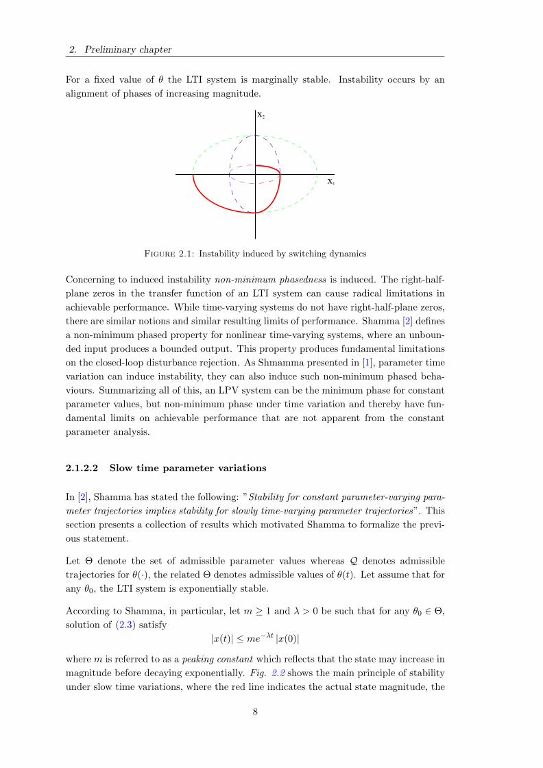
Fig. 2.1 shows the main insight into this problem using the state trajectories of the
LPV system (2.4) with parameter θ which is periodically switching between two values
θ(t) ∈ 〈ωa, ωb〉. In this figure the red line indicates the unstable switching trajectory
and the dashed lines indicate individual oscillatory trajectories.
x =
(0 1
−θ2 0
)x (2.4)
7
2. Preliminary chapter
For a fixed value of θ the LTI system is marginally stable. Instability occurs by an
alignment of phases of increasing magnitude.
x2
x1
Figure 2.1: Instability induced by switching dynamics
Concerning to induced instability non-minimum phasedness is induced. The right-half-
plane zeros in the transfer function of an LTI system can cause radical limitations in
achievable performance. While time-varying systems do not have right-half-plane zeros,
there are similar notions and similar resulting limits of performance. Shamma [2] defines
a non-minimum phased property for nonlinear time-varying systems, where an unboun-
ded input produces a bounded output. This property produces fundamental limitations
on the closed-loop disturbance rejection. As Shmamma presented in [1], parameter time
variation can induce instability, they can also induce such non-minimum phased beha-
viours. Summarizing all of this, an LPV system can be the minimum phase for constant
parameter values, but non-minimum phase under time variation and thereby have fun-
damental limits on achievable performance that are not apparent from the constant
parameter analysis.
2.1.2.2 Slow time parameter variations
In [2], Shamma has stated the following: ”Stability for constant parameter-varying para-
meter trajectories implies stability for slowly time-varying parameter trajectories”. This
section presents a collection of results which motivated Shamma to formalize the previ-
ous statement.
Let Θ denote the set of admissible parameter values whereas Q denotes admissible
trajectories for θ(·), the related Θ denotes admissible values of θ(t). Let assume that for
any θ0, the LTI system is exponentially stable.
According to Shamma, in particular, let m ≥ 1 and λ > 0 be such that for any θ0 ∈ Θ,
solution of (2.3) satisfy
|x(t)| ≤ me−λt |x(0)|
where m is referred to as a peaking constant which reflects that the state may increase in
magnitude before decaying exponentially. Fig. 2.2 shows the main principle of stability
under slow time variations, where the red line indicates the actual state magnitude, the
8
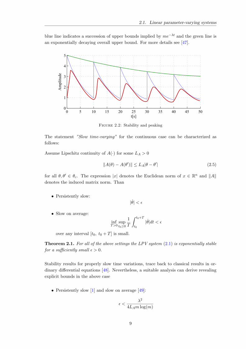
2.1. Linear parameter-varying systems
blue line indicates a succession of upper bounds implied by me−λt and the green line is
an exponentially decaying overall upper bound. For more details see [47].
0 5 10 15 20 25 30 35 40 45 500
1
2
3
4
5
t[s]
Amplitude
Figure 2.2: Stability and peaking
The statement ”Slow time-varying” for the continuous case can be characterized as
follows:
Assume Lipschitz continuity of A(·) for some LA > 0
‖A(θ)−A(θ′)‖ ≤ LA|θ − θ′| (2.5)
for all θ, θ′ ∈ θc. The expression |x| denotes the Euclidean norm of x ∈ Rn and ‖A‖denotes the induced matrix norm. Than
• Persistently slow:
|θ| < ε
• Slow on average:
infT>0
supt0≥0
1
T
∫ t0+T
t0
|θ|dt < ε
over any interval [t0, t0 + T ] is small.
Theorem 2.1. For all of the above settings the LPV system (2.1) is exponentially stable
for a sufficiently small ε > 0.
Stability results for properly slow time variations, trace back to classical results in or-
dinary differential equations [48]. Nevertheless, a suitable analysis can derive revealing
explicit bounds in the above case
• Persistently slow [1] and slow on average [49]:
ε <λ2
4LAm log(m)
9
2. Preliminary chapter
Shamma stated an interesting implication from the above bounds, time variations can
be arbitrarily fast, when m = 1. In terms of the previous discussion, m = 1 implies that
trajectories in the constant parameter case have no peaking, and therefore cannot align
to produce instability.
2.1.2.3 Arbitrary time parameter variations
This section deals with the stability question from the other extreme, when time vari-
ations are arbitrarily fast. For this discussion consider an LPV plant in the form
x(t) = A(θ(t))x(t) (2.6)
Shamma and others [50–52] concluded that
• Determining whether solutions of (2.6) are bounded is undecidable.
• Determining whether (2.6) is asymptotically stable is NP-hard 1
• Consequentially, deriving efficient algorithms for assessing stability will remain to
be elusive.
Shamma according that a consequence of the complexity results is, that one must settle
for non-definitive methods or inefficient algorithms to access stability.
Theorem 2.2. The LPV system (2.1) is exponentially stable for all θ ∈ Ω if there exist
symmetric, positive defined matrix P such that the following inequality holds
AT (θ)P + PA(θ) < 0 (2.7)
The proof is, that xTPx is a Lyapunov function for the LPV system, which in this
case is the only Lyapunov function for all associated constant parameter LTI system.
The result is only a sufficient condition. Shamma in [2] introduced a simple example
from [53] which explains this problem. Consider a simple second-order system whose
dynamics matrix can switch between two matrices
x ∈ A1x, A2x (2.8)
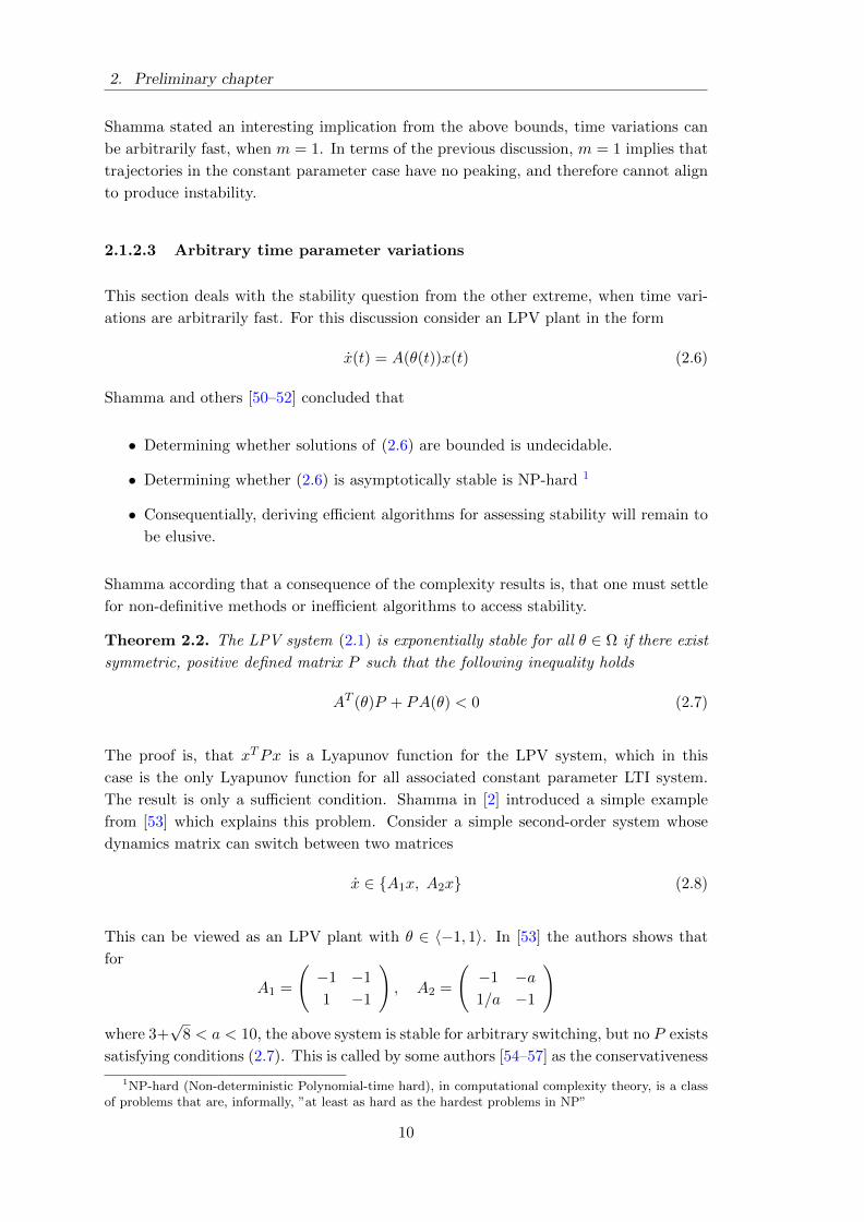
This can be viewed as an LPV plant with θ ∈ 〈−1, 1〉. In [53] the authors shows that
for
A1 =
(−1 −1
1 −1
), A2 =
(−1 −a1/a −1
)where 3+
√8 < a < 10, the above system is stable for arbitrary switching, but no P exists
satisfying conditions (2.7). This is called by some authors [54–57] as the conservativeness
1NP-hard (Non-deterministic Polynomial-time hard), in computational complexity theory, is a classof problems that are, informally, ”at least as hard as the hardest problems in NP”
10
2.1. Linear parameter-varying systems
of the quadratic stability. Therefore a lot of people were looking for a solution on how to
reduce the conservatism. And this has resulted in certain special structures of suitable
Lyapunov functions [54–60].
Let denote
A(t, τ ; θ([τ, t])) (2.9)
as the state transition matrix for an LPV system, where the dependence on the parameter
trajectory is explicit (over the interval [τ, t]). Accordingly
x(t) = A(t, τ ; θ([τ, t]))x(τ) (2.10)
Assuming that an LPV plant is exponentially stable for all parameter trajectories, there
exist m and λ > 0 such that
‖A(t, τ ; θ([τ, t]))‖ ≤ me−λ(t−τ) (2.11)
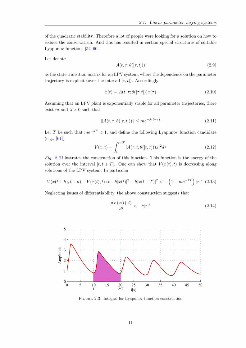
Let T be such that me−λT < 1, and define the following Lyapunov function candidate
(e.g., [61])
V (x, t) =
∫ t+T
t|A(τ, t; θ([t, τ ]))x|2dτ (2.12)
Fig. 2.3 illustrates the construction of this function. This function is the energy of the
solution over the interval [t, t + T ]. One can show that V (x(t), t) is decreasing along
solutions of the LPV system. In particular
V (x(t+ h), t+ h)− V (x(t), t) ≈ −h|x(t)|2 + h|x(t+ T )|2 < −(
1−me−λT)|x|2 (2.13)
Neglecting issues of differentiability, the above construction suggests that
dV (x(t), t)
dt< −c|x|2 (2.14)
0 5 10 15 20 25 30 35 40 45 500
1
2
3
4
5
t[s]
Amplitude
t t+T
Figure 2.3: Integral for Lyapunov function construction
11
2. Preliminary chapter
The structure of this Lyapunov function can be rewritten as a quadratic function in x,
where the defining matrix is a function of the future parameter trajectory
V (x(t), t) = xT (t)P (θ([t, t+ T ]))x(t) (2.15)
We can reparametrize the function to be a function of past parameter trajectories
V (x(t), t) = xT (t)P (θ([t− T, t]))x(t) (2.16)
The authors in [59] used a similar construction to derive the following theorem
Theorem 2.3. [59] An LPV system is exponentially stable for arbitrary time variations
if and only if there exists a trajectory dependent quadratic Lyapunov function of the form
V (x, t) = xTP (θ([t− T, t]))x (2.17)
In discrete time, authors [59] use this result to derive a numerical search for Lyapunov
functions. Regarding the previous discussion on complexity, this search may need to
admit progressively longer intervals of trajectory dependence.
It turns out that one can eliminate the dependence on the parameter trajectory alto-
gether. The intuition is as follows. From the Lyapunov function in Theorem 2.3, define
V (x) = infθ([t−T,t])
xTP (θ([t− T, t]))x (2.18)
The new Lyapunov function is the former Lyapunov function evaluated at a worst case
trajectory [2]. Again, an informal analysis illustrates that this parameter-independent
Lyapunov function decreases along the solution of the LPV system for all parameter
trajectories. This motivates the existence in general of a pseudo-quadratic Lyapunov
function.
Authors Molchanov and Pyatnitskiy in [60] introduced the following theorem
Theorem 2.4. [60] An LPV system is exponentially stable for arbitrary time variations
if and only if there exists a Lyapunov function of the form
V (x) = xTP (x)x (2.19)
for some family of matrices P (·), with the property that P (αx) = αP (x) for α ≥ 0.
In book [2], papers [62, 63], survey [64] and monograph [65] we can find further discus-
sions which go on to characterize alternative piecewise linear structures for exponentially
stable LPV systems. Besides these we can find papers which investigate the stability of
an LPV systems using parameter-dependent quadratic stability [54, 56, 57, 66, 67]. The
main principle of parameter-dependent quadratic stability is that against the result with
quadratic stability we have one Lyapunov function for all vertices of θ. So the Lyapunov
function is parameter-dependent
V (θ(t)) = xT (t)P (θ(t))x(t) (2.20)
12

2.2. Gain scheduling
where θ ∈ Ω and
P (θ) = P0 +
p∑i=1
Piθi (2.21)
P. Gahinet, P. Apkarian and M. Chilali in [57] in this context introduced the following
theorem
Theorem 2.5. [57] The LPV system (2.1) for θ ∈ Ω and θ ∈ Ωt is affinely quadratically
stable if and only if there exist p+ 1 symmetric matrices P0, P1, . . . , Pp such that
P (θ) = P0 +
p∑i=1
Piθi > 0 (2.22)
and for the first derivative of Lyapunov function V (θ) = xTP (θ)x along the trajectory
of LPV system (2.1) it holds
dV (x, θ)
dt= xT
(A(θ)TP (θ) + P (θ)A(θ) +
dP (θ)
dt
)x < 0 (2.23)
wheredP (θ)
dt=
p∑i=1
Piθi ≤p∑i=1
Piρi
In this case we must have predefined the maximum rate of change of scheduled para-
meters θi as ρi.
2.1.3 Summary
In this section (Linear parameter-varying system) the LPV systems were presented and
described and their stability analysis since its introduction (1988 by Jeff. S. Shamma
[1]) to the present (2015). The analysis and theorems stated herein are presented in
an informal manner. Technical details may (and should) be found in the associated
references.
2.2 Gain scheduling
The robust control theory is well established for linear systems but almost all real pro-
cesses are more or less nonlinear. If the plant operating region is small, one can use
the robust control approaches to design a linear robust controller where the nonlinear-
ities are treated as model uncertainties. However, for real nonlinear processes, where
the operating region is large, the above mentioned controller synthesis may be inap-
plicable. For this reason the controller design for nonlinear systems is nowadays a very
determinative and important field of research.
13
2. Preliminary chapter
Gain scheduling is one of the most common used controller design approaches for non-
linear systems and has a wide range of use in industrial applications. In this section
the main principles, several classical approaches and finally the linear parameter-varying
based version of gain scheduling are presented and investigated.
2.2.1 Introduction to gain scheduling
In literature a lot of term are meant under gain scheduling (GS). For example switching
or blending of gain values of controllers or models, switching or blending of complete
controllers or models or adapt (schedule) controller parameters or model parameters ac-
cording to different operating conditions. A common feature is the sense of decomposing
nonlinear design problems into linear or nonlinear sub-problems. The main difference
lies in the realization.
Consequently gain scheduling may be classified in different way
• According to decomposition
1. GS methods decomposing nonlinear design problems into linear sub-problems
2. GS methods decomposing nonlinear design problems into nonlinear (affine)
sub-problems
• According to signal processing
1. Continuous gain scheduling methods
2. Discrete gain scheduling methods
3. hybrid or switched gain scheduling methods
• According to main approaches
1. Classical (linearization based) gain scheduling
2. LFT based GS synthesis
3. LPV based GS synthesis
4. Fuzzy GS techniques
5. Other modern GS techniques
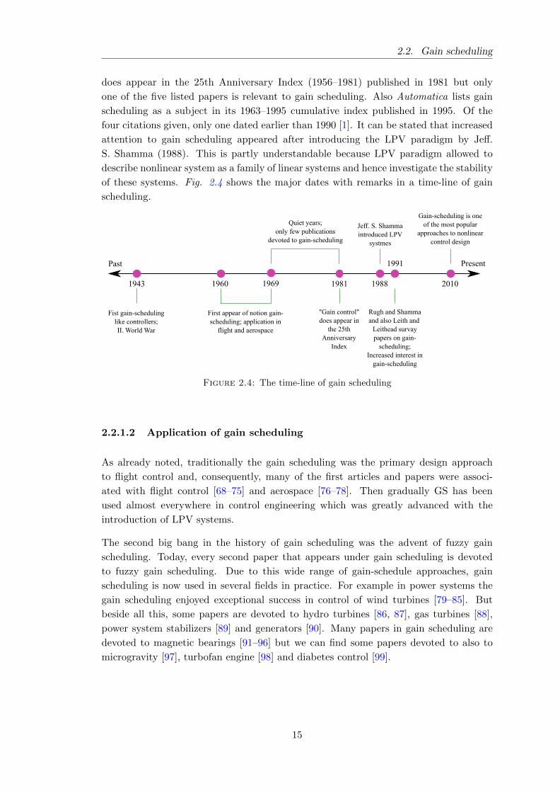
2.2.1.1 History of gain scheduling
The ferret in the history of gain scheduling appears in the 1960s but a similar simpler
technique was used in World War II toat control the rockets V2 (switching controllers
based on measured data). It is not surprising therefore that gain scheduling as a concept
or notion firstly appear in flight control and later in aerospace. Leith and Leithead in
their survey [9] and likewise also Rugh and Shamma in their survey paper [10] considered
the first appearance of GS from the 1960s. Rugh stated in his survey that ”Gain control”
14
2.2. Gain scheduling
does appear in the 25th Anniversary Index (1956–1981) published in 1981 but only
one of the five listed papers is relevant to gain scheduling. Also Automatica lists gain
scheduling as a subject in its 1963–1995 cumulative index published in 1995. Of the
four citations given, only one dated earlier than 1990 [1]. It can be stated that increased
attention to gain scheduling appeared after introducing the LPV paradigm by Jeff.
S. Shamma (1988). This is partly understandable because LPV paradigm allowed to
describe nonlinear system as a family of linear systems and hence investigate the stability
of these systems. Fig. 2.4 shows the major dates with remarks in a time-line of gain
scheduling.
PresentPast
1960 1969 1981 1988
1991
1943
Fist gain-scheduling
like controllers;
II. World War
First appear of notion gain-
scheduling; application in
flight and aerospace
Quiet years;
only few publications
devoted to gain-scheduling
"Gain control"
does appear in
the 25th
Anniversary
Index
Jeff. S. Shamma
introduced LPV
systmes
Rugh and Shamma
and also Leith and
Leithead survay
papers on gain-
scheduling;
Increased interest in
gain-scheduling
Gain-scheduling is one
of the most popular
approaches to nonlinear
control design
2010
Figure 2.4: The time-line of gain scheduling
2.2.1.2 Application of gain scheduling
As already noted, traditionally the gain scheduling was the primary design approach
to flight control and, consequently, many of the first articles and papers were associ-
ated with flight control [68–75] and aerospace [76–78]. Then gradually GS has been
used almost everywhere in control engineering which was greatly advanced with the
introduction of LPV systems.
The second big bang in the history of gain scheduling was the advent of fuzzy gain
scheduling. Today, every second paper that appears under gain scheduling is devoted
to fuzzy gain scheduling. Due to this wide range of gain-schedule approaches, gain
scheduling is now used in several fields in practice. For example in power systems the
gain scheduling enjoyed exceptional success in control of wind turbines [79–85]. But
beside all this, some papers are devoted to hydro turbines [86, 87], gas turbines [88],
power system stabilizers [89] and generators [90]. Many papers in gain scheduling are
devoted to magnetic bearings [91–96] but we can find some papers devoted to also to
microgravity [97], turbofan engine [98] and diabetes control [99].
15
2. Preliminary chapter
2.2.2 Classical gain scheduling
In the case of nonlinear dynamics an idea is widely used among control engineers to
linearize the plant around several operating points and to use linear control tools to
design a controller for each of these points. The actual controller is implemented using
the gain scheduling approach. Success of such an approach depends on establishing the
relationship between a nonlinear system and a family of linear ones. There are two main
problems:
1. Stability results: stability of the closed-loop nonlinear system and of the closed-
loop family of linear systems, when scheduled parameters are changes.
2. Approximation results which provide a direct relationship between the solution of
closed-loop nonlinear systems and the solution of associated linear systems [10],
[9]
Rugh and Shamma in [10] comprise four main steps in classical gain scheduling
1. A family of LTI approximations are obtained from nonlinear plant at constant
operating points (equilibria), parametrized by exogenous signal θ (scheduled para-
meter) which is computed using linearization based scheduling. The linearization
has to correspond to zero error. Other syntheses to derive a parameter-dependent
model are
• Off-equilibrium or velocity based linearization [9, 100–102] - when zero equi-
librium points or working conditions are not present
• Quasi LPV approach [9, 10, 102], in which the plant dynamics are rewrit-
ten to distinguish nonlinearities as time-varying parameters that are used as
scheduling variables.
• Direct LPV modelling, based on a linear plant incorporating time-varying
parameters [1, 75, 102] - when no nonlinear plant is involved. This also
includes black-box or data-based modelling methods
2. A set of LTI controllers are designed using linear control tools for previously derived
set of local LTI models to achieve specified performance and stability at each
operating point. The resulting set of controllers is also parametrized by scheduled
parameter θ. Although the scheduled parameter is time-varying, the classical gain
scheduling methods are based on fixed or frozen scheduling parameter values. To
enable subsequent scheduling, interpolation of controller parameters, the set of LTI
controllers almost requires a fixed structure of the controller design. Exceptions
are
• in the case direct derivation of a Linear Parameter-Varying (LPV) control-
ler for a corresponding LPV plant model is possible, subsequent scheduling,
interpolation becomes superfluous.
16
2.2. Gain scheduling
• when discrete or hybrid scheduling instead of continuous scheduling is deman-
ded, the set of controller designs not necessarily need to be fixed-structured.
3. Implementation of the family of LTI controllers such that the controller coefficients
are scheduled according to the current value of the scheduling variable, e.g. by
controller gain interpolation or scheduling. At this point, θ = θ(t) is implemented.
At each operating point, the scheduled controller has to be linearized to the corres-
ponding linear controller design as well as provide a constant control value yielding
zero error at these points. As mentioned in Step 2, in the case of direct scheduling,
this step becomes superfluous. Furthermore, in the case of discrete scheduling, the
implementation of the LTI controllers involves the design of a scheduled selection
procedure that is applied to the set of LTI controllers, rather than the design of
a family of scheduled controllers. The presence of hidden coupling terms is an
important aspect which yields various additional requirements to the scheduling
procedure.
4. Typically, local performance assessment can be performed analytically, whereas
assessment of global performance and robustness has to be established by extensive
simulations. Non-local performance of the gain-scheduled controller is evaluated
and checked by simulations.
2.2.3 LFT and LPV based gain scheduling
The LPV and LFT syntheses are based on LPV and LFT plant representations respect-
ively (Naus [102]). Both methods yield direct synthesis of a controller utilizing (L2
or H∞) norm based methods, with guarantees the robustness, performance and nom-
inal stability of the overall gain-scheduled design [7, 57, 66, 102–104]. LPV and LFT
syntheses essentially involve only two main steps.
1. The first step corresponds to the classical approach. A family of LTI approxima-
tions of a nonlinear plant at constant operating points (equilibria), parameterized
by constant values of convenient plant variables or exogenous signals θ are com-
puted. Subsequent implementation of the controller requires θ = θ(t) to be a
measurable variable. Besides the already mentioned methods, which all arrive at
Linear Parameter-Varying (LPV) models, in specific cases a LFT description is
possible. The LFT description serves as a basis for subsequent LFT controller
synthesis.
2. LPV and LFT control synthesis directly yield a gain-scheduled controller. Stability
and performance specifications can be guaranteed a priori as the time-varying
parameter θ(t) instead of its corresponding frozen value θ is addressed in the
design process. In [102] one can find only continuous-time gain scheduling but
the author Sato in 2011 [105] introduced discrete-time version of LPV based gain
scheduling where stability investigated with both H2 and H∞.
17
2. Preliminary chapter
2.2.3.1 LPV gain scheduling
The main advantages of the LPV control synthesis are as follows (Naus [102])
• There exists a solid theoretical foundation guaranteeing a priori stability and per-
formance for all θ(t) given a corresponding range and rate of variation of θ(t)
• The corresponding controller design is global with respect to the parametrized
operating envelope Ω, Ωt, whereas classical gain scheduling techniques focus on
local system properties.
• A controller is synthesized directly, rather than its construction from a family of
local linear controllers.
The main disadvantages are
• with respect to classical gain scheduling techniques, the controller synthesis is much
more involved, which results in focusing on appropriate problem formulation rather
than the actual controller design
• generally, conservatism has to be introduced to arrive at a feasible and convex
problem
• with respect to classical gain scheduling, allowing for arbitrary linear controller
design techniques, a predefined controller design synthesis has to be adopted.
As the latter point already indicates, LPV syntheses constitutes a specific performance
evaluation framework, whereas classical gain scheduling provides an open framework.
Typically, LPV syntheses employ the induced L2-norm as a performance measure, which
is directly related to linear H∞ techniques. As a result, an LPV control synthesis applied
to a time-invariant system is equivalent to a standard H∞ approach. In general, LPV
control syntheses can be categorized into
1. Lyapunov-based approach (LPV-based techniques)
2. techniques exploiting the specific structure of systems with LFT parameter de-
pendence, utilizing a small-gain approach, which are also determined as LFT ap-
proaches
3. a combination of the two preceding points, which Naus referred as ‘mixed’ LPV-
LFT approaches
18
2.2. Gain scheduling
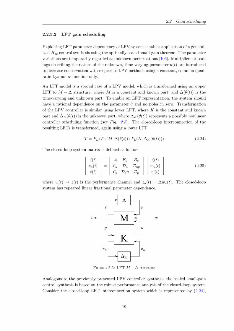
2.2.3.2 LFT gain scheduling
Exploiting LFT parameter-dependency of LPV systems enables application of a general-
ized H∞ control synthesis using the optimally scaled small-gain theorem. The parameter
variations are temporarily regarded as unknown perturbations [106]. Multipliers or scal-
ings describing the nature of the unknown, time-varying parameter θ(t) are introduced
to decrease conservatism with respect to LPV methods using a constant, common quad-
ratic Lyapunov function only.
An LFT model is a special case of a LPV model, which is transformed using an upper
LFT to M − ∆ structure, where M is a constant and known part, and ∆(θ(t)) is the
time-varying and unknown part. To enable an LFT representation, the system should
have a rational dependence on the parameter θ and no poles in zero. Transformation
of the LPV controller is similar using lower LFT, where K is the constant and known
part and ∆K(θ(t)) is the unknown part, where ∆K(θ(t)) represents a possibly nonlinear
controller scheduling function (see Fig. 2.5). The closed-loop interconnection of the
resulting LFTs is transformed, again using a lower LFT
T = FL (FU (M,∆(θ(t))) FL(K,∆K(θ(t)))) (2.24)
The closed-loop system matrix is defined as follows ζ(t)
zu(t)
z(t)
=
A Bu BpCu Du DupCp Dpu Dp
ζ(t)
wu(t)
w(t)
(2.25)
where w(t) → z(t) is the performance channel and zu(t) = ∆wu(t). The closed-loop
system has repeated linear fractional parameter dependence.
∆
∆K
M
K
vr
wz
uy
vKrK
Figure 2.5: LFT M −∆ structure
Analogous to the previously presented LPV controller synthesis, the scaled small-gain
control synthesis is based on the robust performance analysis of the closed-loop system.
Consider the closed-loop LFT interconnection system which is represented by (2.24),
19
2. Preliminary chapter
(2.25). The corresponding analysis involves three main conditions regarding the closed-
loop model T , comprising [107]
• well-posedness, i.e. for all initial conditions corresponding to the augmented sys-
tem M and all inputs w(t) to the system, the system should have a unique solution.
• exponential stability of the closed-loop system, which is analyzed via the small-
gain theory, which states that a closed-loop system is stable provided that the
loop-gain is less than unity
• performance; (quadratic performance or L2-performance or . . .)
Combining all three conditions we obtain a set of LMIs, which is directly derived from
the general LPV synthesis constraints [108].
The main advantages of the LFT approach are the possibility to use the optimally
scaled small-gain theorem, which is well-established in literature, and the possibility to
arrive at a finite dimensional set of LMIs using multipliers. However, the general full-
block multiplier approach is complex, whereas relaxations on the multipliers introduce
(much) conservatism. Furthermore, the use of a constant, common quadratic Lyapunov
function, implying that infinitely fast parameter variations are accounted for, introduces
conservatism, especially in the case of large parameter variations. Finally, the controller
inherits the LFT parameter dependency, which might be conservative, and possible
realness of the parameter θ(t) is not exploited, introducing conservatism as well.
2.2.4 Fuzzy gain scheduling
Fuzzy gain scheduling should overcome the disadvantage of classical gain scheduling
regarding the restriction of stability and performance analysis to local rather than global
closed-loop behaviour [70, 88, 96, 102]. The corresponding fuzzy modelling considers the
transient dynamics of the original nonlinear model instead of local linearizations only.
Fuzzy gain scheduling techniques may involve classical gain scheduling alike as well as
LPV techniques. According to Naus [102], focusing on the former one, four main steps
have to be considered.
1. Analogous to classical gain scheduling, sets of local LTI models and corresponding
LTI controllers have to be designed. Focus lies on the regions of the envelope
of operating conditions for which these controllers assure stability and desired
performance of the resulting (local) closed-loop systems.
2. To arrive at a fuzzy model, so-called weighting or scaling functions are designed,
corresponding to the before mentioned regions. Utilizing these weighting functions,
the local models are blended. Specifying a specific approximation accuracy of
the fuzzy model with respect to the original nonlinear model, yields the required
number of local models.
20
2.2. Gain scheduling
3. The set of local controllers is blended analogous to the set of local models. The
same weighting functions are utilized. The blending yields scheduling of the con-
troller outputs rather than scheduling of the controllers or controller coefficients.
Hence, members of the corresponding parameterized set of LTI controllers do not
necessarily need to have fixed structure and dimension.
4. Stability and performance are established by extensive simulations, analogous to
classical gain scheduling. However, in the case of fuzzy controller design, global as
well as local specifications have to be derived from simulations, as the characteristic
dynamics of the fuzzy model can not be related to the dynamics of the set of local
models.
2.2.5 Summary
This section deals with gain scheduling and gain-scheduled controller designs (classical
gain scheduling, LPV and LFT based gain scheduling and fuzzy gain scheduling).
The main advantage of classical gain scheduling is that it inherits the benefits of lin-
ear controller design methods, including intuitive classical design tools and time as well
as frequency domain performance specifications. PID control is the most used control
strategy in industrial applications due to its relatively simple and intuitive design, hence
this is a major advantage with respect to other nonlinear controller design syntheses.
The approach thus enables the design of low computational effort controllers. Concep-
tually, gain scheduling involves an intuitive simplification of the problem into parallel
decompositions of the total system.
LPV and LFT synthesis require a true LPV model as a basis. In general however, gain
scheduling may be employed in the absence of an analytical model, e.g. on the basis of
a collection of plant linearizations. Consequently, controller design based on a whitebox
as well as a blackbox and even data-based ’modeling’ is possible. If the possibility of
fast parameter variations is not addressed in the design process, guaranteed properties
of the overall gain-scheduled design cannot be established. The main advantage of LPV
and LFT control synthesis is that they do account for parameter variations in the con-
troller design, which results in a priori guarantees regarding stability and performance
specifications. The main drawback of LPV and LFT control synthesis involves conser-
vativeness, which has to be introduced to enable solving the resulting LMIs. As a result
of that, current LPV and LFT syntheses comprise specific extensions of robust control
techniques rather than true generalizations. However, current and future research still
provides and will provide less conservative solutions.
The main drawback of fuzzy gain scheduling involves the lack of a relation between
the dynamic characteristics of the original nonlinear model and the fuzzy model. Even
locally, the dynamics of the fuzzy model can not be related to the original nonlinear
model. Fuzzy gain scheduling techniques may involve classical gain scheduling alike as
well as LPV techniques.
21
2. Preliminary chapter
The analysis and theorems stated herein are presented in an informal manner. Technical
details may (and should) be found in the associated references.
2.3 Discussion
This thesis is devoted to gain scheduling within this to LPV based gain scheduling
because in our opinion the biggest potential between gain scheduling approaches is in the
LPV based gain scheduling. Despite this, we described all main historical approaches to
gain scheduling as classical gain scheduling, LFT based gain scheduling and novel fuzzy
gain scheduling.
As we mentioned LPV based gain scheduling appear in 1988 when Jeff. S. Shamma
introduced the LPV paradigm in his Ph.D. thesis [1]. Today LPV paradigm has become
a standard formalism in systems and controls with lots of researches and articles devoted
to analysis, controller design and system identification of these models. Due to this
nowadays the LPV gain scheduling belongs to the most popular approaches to nonlinear
control design. But, as we mentioned in Chapter 1, there are still a lot of unsolved
problems. Browsing through literature we cannot find any general LPV based gain-
scheduled approach which will involve guaranteed cost and affine quadratic stability. In
addition there are very rudimentary approaches in switched and predictive control not
to mention the robust and discrete design approaches.
Currently, nowhere it is solved how to affect the performance quality separately in each
working point when direct LPV controller approach is used. Furthermore, there are
only few papers devoted to output feedbacks and they also not use fixed order output
feedbacks like PID/PSD controllers.
Most of the papers devoted to LPV based gain scheduling convert the stability condi-
tions into LMI problems. But currently we cannot find a general LMI approach with
guaranteed stability and guaranteed cost. Furthermore, nowhere it is solved how to
consider input/output constraints without need of on-line optimization.
Among other things, to find a solution for some of these unsolved problems (deficiencies)
were the main goals of the research which is summarized in this thesis.
Bibliography
[1] J. S. Shamma, Analysis and design of gain scheduled control systems, Phd thesis,
Massachusetts Institute of Technology, Department of Mechanical Engineering,
advised by M. Athans (1988).
[2] J. S. Shamma, Control of Linear Parameter Varying Systems with Applications,
Springer, 2012, Ch. An overview of LPV systems, pp. 3–26.
[3] D. A. Lawrence, W. J. Rugh, Gain scheduling dynamic linear controllers for a
nonlinear plant, Automatica 31 (3) (1995) 381–390.
22
Bibliography
[4] W. Rugh, Analytical framework for gain scheduling, IEEE Control Systems 11 (1)
(1991) 79–84.
[5] J. S. Shamma, The Control Handbook, CRC Press, Inc, Boca Raton, FL, 1996,
Ch. Linearization and gain-scheduling, pp. 388–398.
[6] J. S. Shamma, Encyclopedia of electrical and electronics engineering, John Wiley
& Sons, New York, 1999, Ch. Gain-scheduling.
[7] J. S. Shamma., M. Athans, Analysis of nonlinear gain scheduled control systems,
IEEE Transactions in Automative Control 35 (8) (1990) 898–907.
[8] J. Shamma, M. Athans, Gain scheduling: potential hazards and possible remedies,
IEEE Control Systems 12 (3) (1992) 101–107.
[9] D. J. Leith, W. E. Leithead, Survey of gain-scheduling analysis and design, Inter-
national Journal of Control 73 (11) (2000) 1001–1025.
[10] W. J. Rugh, J. S. Shamma, Survey Research on gain scheduling, Automatica
36 (10) (2000) 1401–1425.
[11] G. Balas, I. Fialho, A. Packard, J. Renfrow, C. Mullaney, On the design of LPV
controllers for the F-14 aircraft lateral-directional axis during powered approach,
in: Proceedings of the 1997 American Control Conference, Vol. 1, 1997, pp. 123–
127.
[12] L. H. Carter, J. S. Shamma, Gain Scheduled Bank-to-Turn Autopilot Design Using
Linear Parameter Varying Transformations, Journal of Guidance, Control, and
Dynamics 19 (5) (1996) 1056–1063.
[13] S. Ganguli, A. Marcos, G. Balas, Reconfigurable LPV control design for Boe-
ing 747-100/200 longitudinal axis, in: Proceedings of the 2002 American Control
Conference, Vol. 5, 2002, pp. 3612–3617.
[14] B. Lu, F. Wu, S. Kim, Switching LPV control of an F-16 aircraft via controller
state reset, IEEE Transactions on Control Systems Technology 14 (2) (2006) 267–
277.
[15] G. Papageorgiou, K. Glover, G. D’Mello, Y. Patel, Taking robust lpv control into
flight on the vaac harrier, in: Proceedings of the 39th IEEE Conference on Decision
and Control, Vol. 5, 2000, pp. 4558–4564.
[16] J. S. Shamma, J. R. Cloutier, Gain-scheduled missile autopilot design using linear
parameter varying transformations, Journal of Guidance, Control, and Dynamics
16 (2) (1993) 256–264.
[17] W. Tan, A. K. Packard, G. Balas, Quasi-lpv modeling and lpv control of a generic
missile, in: Proceedings of the American Control Conference, Vol. 5, 2000, pp.
3692–3696.
23
2. Preliminary chapter
[18] J. M. Barker, G. J. Balas, Comparing Linear Parameter-Varying Gain-Scheduled
Control Techniques for Active Flutter Suppression, in: Journal of Guidance, Con-
trol, and Dynamics, Vol. 23, American Institute of Aeronautics and Astronautics,
2000, pp. 948–955.
[19] A. Jadbabaie, J. Hauser, Control of a thrust-vectored flying wing: a receding
horizon – LPV approach, International Journal of Robust and Nonlinear Control
12 (9) (2002) 869–896.
[20] E. Lau, A. Krener, LPV control of two dimensional wing flutter, in: Proceedings of
the 38th IEEE Conference on Decision and Control, Vol. 3, 1999, pp. 3005–3010.
[21] J. van Wingerden, P. Gebraad, M. Verhaegen, Lpv identification of an aeroelastic
flutter model, in: 49th IEEE Conference on Decision and Control (CDC), 2010,
pp. 6839–6844.
[22] G. J. Balas, Linear, parameter-varying control and its application to a turbofan
engine, International Journal of Robust and Nonlinear Control 12 (9) (2002) 763–
796.
[23] F. Bruzelius, C. Breitholtz, S. Pettersson, LPV-based gain scheduling technique
applied to a turbo fan engine model, in: Proceedings of the 2002 International
Conference on Control Applications, Vol. 2, 2002, pp. 713–718.
[24] W. Gilbert, D. Henrion, J. Bernussou, D. Boyer, Polynomial LPV synthesis applied
to turbofan engines, Control Engineering Practice 18 (9) (2010) 1077–1083.
[25] L. Shu-qing, Z. Sheng-xiu, A modified LPV modeling technique for turbofan engine
control system, in: International Conference on Computer Application and System
Modeling (ICCASM), Vol. 5, 2010, pp. 99–102.
[26] B. Lu, H. Choi, G. D. Buckner, K. Tammi, Linear parameter-varying techniques
for control of a magnetic bearing system, Control Engineering Practice 16 (10)
(2008) 1161–1172.
[27] J. Witte, H. M. N. K. Balini, C. Scherer, Robust and lpv control of an amb system,
in: American Control Conference (ACC), 2010, pp. 2194–2199.
[28] F. Wu, Switching lpv control design for magnetic bearing systems, in: Proceedings
of the 2001 IEEE International Conference on Control Applications (CCA ’01),
2001, pp. 41–46.
[29] I. Fialho, G. Balas, Road adaptive active suspension design using linear parameter-
varying gain-scheduling, IEEE Transactions on Control Systems Technology 10 (1)
(2002) 43–54.
[30] P. Gaspar, I. Szaszi, J. Bokor, The design of a combined control structure to
prevent the rollover of heavy vehicles, European Journal of Control 10 (2) (2004)
148–162.
24
Bibliography
[31] B. He, M. Yang, Robust lpv control of diesel auxiliary power unit for series hybrid
electric vehicles, IEEE Transactions on Power Electronics 21 (3) (2006) 791–798.
[32] C. Poussot-Vassal, O. Sename, L. Dugard, P. Gaspar, Z. Szabo, J. Bokor, A new
semi-active suspension control strategy through LPV technique, Control Engin-
eering Practice 16 (12) (2008) 1519–1534.
[33] X. Wei, L. Del Re, Gain scheduled h∞ control for air path systems of diesel engines
using lpv techniques, IEEE Transactions on Control Systems Technology 15 (3)
(2007) 406–415.
[34] F. Zhang, K. Grigoriadis, M. Franchek, I. Makki, Linear parameter-varying lean
burn air-fuel ratio control, in: 44th IEEE Conference on Decision and Control and
European Control Conference. CDC-ECC ’05., 2005, pp. 2688–2693.
[35] F. Bianchi, R. Mantz, C. Christiansen, Gain scheduling control of variable-speed
wind energy conversion systems using quasi-LPV models, Control Engineering
Practice 13 (2) (2005) 247–255.
[36] F. Lescher, J. Y. Zhao, P. Borne, Switching LPV controllers for a variable speed
pitch regulated wind turbine, in: IMACS Multiconference on Computational En-
gineering in Systems Applications, 2006, pp. 1334–1340.
[37] G. Mercere, H. Palsson, T. Poinot, Continuous-time linear parameter-varying iden-
tification of a cross flow heat exchanger: A local approach, IEEE Transactions on
Control Systems Technology 19 (1) (2011) 64–76.
[38] P. Lopes dos Santos, T.-P. Azevedo-Perdicoulis, J. Ramos, J. de Carvalho, G. Jank,
J. Milhinhos, An lpv modeling and identification approach to leakage detection in
high pressure natural gas transportation networks, IEEE Transactions on Control
Systems Technology 19 (1) (2011) 77–92.
[39] C. S. Mehendale, I. J. Fialho, K. M. Grigoriadis, A linear parameter-varying frame-
work for adaptive active microgravity isolation, Journal of Vibration and Control
15 (5) (2009) 773–800.
[40] C. Mehendale, I. Fialho, K. Grigoriadis, Adaptive active microgravity isolation
using lpv gain-scheduling methods, in: Proceedings of the 2003 American Control
Conference, Vol. 2, 2003, pp. 1452–1457.
[41] F. Zhang, K. M. Grigoriadis, I. J. Fialho, Linear Parameter-Varying Antiwindup
Compensation for Active Microgravity Vibration Isolation, Journal of Guidance
Control Dynamics 30 (2007) 1062–1067.
[42] R. Pea, A. Ghersin, Lpv control of glucose for diabetes type i, in: Annual In-
ternational Conference of the IEEE Engineering in Medicine and Biology Society
(EMBC), 2010, pp. 680–683.
[43] L. Kovacs, B. Kulcsar, LPV Modeling of Type 1 Diabetes Mellitus, in: 8th Inter-
national Symposium of Hungarian Researchers on Computational Intelligence and
Informatics, 2007, pp. 163–173.
25
2. Preliminary chapter
[44] L. Kovacs, B. Kulcsaar, J. Bokor, Z. Benyo, LPV fault detection of glucose-insulin
system, in: MED ’06. 14th Mediterranean Conference on Control and Automation,
2006, pp. 1–5.
[45] H. H. Lin, C. Beck, M. Bloom, Multivariable lpv control of anesthesia delivery
during surgery, in: American Control Conference, 2008, pp. 825–831.
[46] M. G. Wassink, M. van de Wal, C. Scherer, O. Bosgra, LPV control for a wafer
stage: beyond the theoretical solution, Control Engineering Practice 13 (2) (2005)
231–245.
[47] B. Francis, K. Glover, Bounded peaking in the optimal linear regulator with cheap
control, IEEE Transactions on Automatic Control 23 (4) (1978) 608–617.
[48] C. Desoer, M. Vidyasagar, Feedback systems: input-output properties, Electrical
science series, Academic Press, 1975.
[49] J. Krause, K. Kumar, An alternate stability analysis framework for adaptive con-
trol, Systems & Control Letters 7 (1) (1986) 19–24.
[50] V. D. Blondel, J. N. Tsitsiklis, The boundedness of all products of a pair of matrices
is undecidable, Systems & Control Letters 41 (2) (2000) 135–140.
[51] O. Toker, On the complexity of the robust stability problem for linear parameter
varying systems, Automatica 33 (11) (1997) 2015–2017.
[52] J. N. Tsitsiklis, V. D. Blondel, The lyapunov exponent and joint spectral radius of
pairs of matrices are hard - when not impossible - to compute and to approximate.,
MCSS 10 (1) (1997) 31–40.
[53] W. Dayawansa, C. Martin, A Converse Lyapunov Theorem for a Class of Dynam-
ical Systems which Undergo Switching, IEEE Transactions on Automatic Control
44 (4) (1999) 751–760.
[54] F. Wang, V. Balakrishnan, Improved stability analysis and gain-scheduled control-
ler synthesis for parameter-dependent systems, IEEE Transactions on Automatic
Control 47 (5) (2002) 720–734.
[55] D. Materassi, M. Salapaka, Less conservative absolute stability criteria using in-
tegral quadratic constraints, in: American Control Conferenc (ACC ’09.), 2009,
pp. 113–118.
[56] X. Zhang, P. Tsiotras, T. Iwasaki, Parameter-dependent Lyapunov function for
exact stability analysis of single-parameter dependent LTI systems, in: 42nd IEEE
Conference on Decision and Control, 2003. Proceedings., Vol. 5, 2003, pp. 5168–
5173 Vol.5.
[57] P. Gahinet, P. Apkarian, M. Chilali, Affine parameter-dependent Lyapunov func-
tions and real parametric uncertainty, IEEE Transactions on Automatic Control
41 (3) (1996) 436–442.
26
Bibliography
[58] K. Wulff, Quadratic and Non-Quadratic Stability Criteria for Switched Linear
Systems, Ph.D. Thesis, Department of Computer Science, National University of
Ireland, Maynooth (December 2004).
[59] D. Liberzon, A. Morse, Basic problems in stability and design of switched systems,
IEEE Control Systems 19 (5) (1999) 59–70.
[60] A. Molchanov, Y. Pyatnitskiy, Criteria of asymptotic stability of differential and
difference inclusions encountered in control theory, Systems & Control Letters
13 (1) (1989) 59–64.
[61] W. J., The Analysis of Feedback Systems, MIT Press, Cambridge, MA, 1971.
[62] A. P. Molchanov, E. S. Pyatnitskii, Lyapunov functions specifying necessary and
sufficient conditions of absolute stability of nonlinear nonstationary control system,
part i., Automation and Remote Control 47 (3) (1986) 344–354.
[63] A. P. Molchanov, E. S. Pyatnitskii, Lyapunov functions specifying necessary and
sufficient conditions of absolute stability of nonlinear nonstationary control system,
part ii., Automation and Remote Control 47 (4) (1986) 443–451.
[64] F. Blanchini, Set invariance in control, Automatica 35 (11) (1999) 1747–1767.
[65] F. Blanchini, D. Casagrande, S. Miani, U. Viaro, Stable LPV Realization of Para-
metric Transfer Functions and Its Application to Gain-Scheduling Control Design,
IEEE Transactions on Automatic Control 55 (10) (2010) 2271–2281.
[66] M. Sato, Brief paper: Gain-scheduled output-feedback controllers depending solely
on scheduling parameters via parameter-dependent Lyapunov functions, Automat-
ica 47 (12) (2011) 2786–2790.
[67] H. Koroglu, Robust generalized asymptotic regulation via an LPV controller
without parameter derivative dependence, in: 49th IEEE Conference on Decision
and Control (CDC), 2010, pp. 4965–4971.
[68] Y. Sun, W. Zhang, M. Zhang, D. Li, Design of Neural Network Gain Scheduling
Flight Control Law Using a Modified PSO Algorithm Based on Immune Clone
Principle, in: Second International Conference on Intelligent Computation Tech-
nology and Automation,(ICICTA ’09), Vol. 1, 2009, pp. 259–263.
[69] D. Xinmin, X. zhiguo, L. qin, Gain scheduled model following control of flight
control system based on neural network, in: Proceedings of the 2003 International
Conference on Neural Networks and Signal Processing, Vol. 1, 2003, pp. 301–305.
[70] M. Oosterom, R. Babuska, Fuzzy gain scheduling for flight control laws, in: The
10th IEEE International Conference on Fuzzy Systems, Vol. 2, 2001, pp. 716–719.
[71] I. Masubuchi, J. Kato, M. Saeki, A. Ohara, Gain-scheduled controller design based
on descriptor representation of LPV systems: application to flight vehicle control,
in: 43rd IEEE Conference on Decision and Control,(CDC), Vol. 1, 2004, pp. 815–
820.
27
2. Preliminary chapter
[72] C.-K. Chu, G.-R. Yu, E. Jonckheere, H. Youssef, Gain scheduling for fly-by-throttle
flight control using neural networks, in: Proceedings of the 35th IEEE Conference
on Decision and Control, Vol. 2, 1996, pp. 1557–1562.
[73] R. Adams, A. G. Sparks, S. Banda, A gain scheduled multivariable design for a
manual flight control system, in: First IEEE Conference on Control Applications,
1992, pp. 584–589.
[74] G. hong Yang, K.-Y. Lum, Gain-scheduled flight control via state feedback, in:
Proceedings of the 2003 American Control Conference, Vol. 4, 2003, pp. 3484–
3489 vol.4.
[75] R. A. Nichols, R. T. Reichert, W. J. Rugh, Gain Scheduling for h∞ Controllers:
A Flight Control Example, IEEE Transactions on Control Systems Technology 1
(1993) 69–79.
[76] C. H. Lee, M.-J. Chung, Gain-scheduled state feedback control design technique
for flight vehicles, IEEE Transactions on Aerospace and Electronic Systems 37 (1)
(2001) 173–182.
[77] X. Huang, Q. Wang, Y. Wang, Y. Hou, C. Dong, Adaptive augmentation of gain-
scheduled controller for aerospace vehicles, Journal of Systems Engineering and
Electronics 24 (2) (2013) 272–280.
[78] R. Hyde, K. Glover, The application of scheduled h∞ controllers to a VSTOL
aircraft, IEEE Transactions on Automatic Control 38 (7) (1993) 1021–1039.
[79] J. jun Chen, Z. cheng Ji, The gain scheduling control for wind energy conversion
system based on lpv model, in: International Conference on Networking, Sensing
and Control (ICNSC), 2010, pp. 653–657.
[80] H. Badihi, Y. Zhang, H. Hong, Fault-tolerant control design for a large off-shore
wind turbine using fuzzy gain-scheduling and signal correction, in: American Con-
trol Conference (ACC), 2013, pp. 1448–1453.
[81] X. Liu, R. Wang, X. Zhang, D. Xu, Gain scheduling pd controller for variable
pitch wind turbines, in: 7th International Power Electronics and Motion Control
Conference (IPEMC), Vol. 3, 2012, pp. 2162–2167.
[82] W. Wang, D. Wu, Y. Wang, Z. Ji, h∞ gain scheduling control of pmsg-based wind
power conversion system, in: The 5th IEEE Conference on Industrial Electronics
and Applications (ICIEA), 2010, pp. 712–717.
[83] K. Ostergaard, P. Brath, J. Stoustrup, Gain-scheduled linear quadratic control of
wind turbines operating at high wind speed, in: IEEE International Conference
on Control Applications (CCA), 2007, pp. 276–281.
[84] F. Bianchi, H. De Battista, R. Mantz, Optimal gain-scheduled control of fixed-
speed active stall wind turbines, Renewable Power Generation, IET 2 (4) (2008)
228–238.
28
Bibliography
[85] W. Ding-Hui, L. Yi-Yang, S. Yan-Xia, J. Zhi-Cheng, Lpv robust gain-scheduling
control for doubly fed induction generator wind energy conversion system, in: 31st
Chinese Control Conference (CCC), 2012, pp. 6687–6691.
[86] G. Ruzhekov, T. Slavov, T. Puleva, Modeling and implementation of hydro turbine
power adaptive control based on gain scheduling technique, in: 16th International
Conference on Intelligent System Application to Power Systems (ISAP), 2011, pp.
1–6.
[87] V. Ginter, J. Pieper, Robust Gain Scheduled Control of a Hydrokinetic Turbine
Part 2: Testing, in: IEEE Electrical Power Energy Conference (EPEC), 2009, pp.
1–5.
[88] A. Rodriguez-Martinez, R. Garduno-Ramirez, PI fuzzy gain-scheduling speed con-
trol of a gas turbine power plant, in: Proceedings of the 13th International Con-
ference on Intelligent Systems Application to Power Systems, 2005, p. 6.
[89] F. Ghosh, Design and Performance of a Local Gain Scheduling Power System
Stabilizer for Inter-Connected System, in: TENCON ’91 IEEE Region 10th In-
ternational Conference on EC3-Energy, Computer, Communication and Control
Systems, Vol. 1, 1991, pp. 355–359.
[90] R. Mohammadi-Milasi, M. Yazdanpanah, P. Jabehdar-Maralani, A novel adaptive
gain-scheduling controller for synchronous generator, in: Proceedings of the 2004
IEEE International Conference on Control Applications, Vol. 1, 2004, pp. 800–805.
[91] C. Knospe, C. Yang, Gain-scheduled control of a magnetic bearing with low bias
flux, in: Proceedings of the 36th IEEE Conference on Decision and Control, Vol. 1,
1997, pp. 418–423 vol.1.
[92] A. Mohamed, I. Hassan, A. Hashem, Application of discrete-time gain-scheduled
q-parameterization controllers to magnetic bearing systems with imbalance, in:
Proceedings of the 1999 American Control Conference, Vol. 1, 1999, pp. 598–602
vol.1.
[93] S. Sivrioglu, K. Nonami, LMI approach to gain scheduled h∞ control beyond PID
control for gyroscopic rotor-magnetic bearing system, in: Proceedings of the 35th
IEEE Conference on Decision and Control, Vol. 4, 1996, pp. 3694–3699.
[94] F. Matsumura, T. Namerikawa, K. Hagiwara, M. Fujita, Application of gain sched-
uled h∞ robust controllers to a magnetic bearing, IEEE Transactions on Control
Systems Technology 4 (5) (1996) 484–493.
[95] F. Betschon, C. Knospe, Reducing magnetic bearing currents via gain scheduled
adaptive control, IEEE/ASME Transactions on Mechatronics 6 (4) (2001) 437–
443.
[96] S. Lei, A. Palazzolo, A. Kascak, Fuzzy Logic Intelligent Control System of Mag-
netic Bearings, in: FUZZ-IEEE 2007, IEEE International Fuzzy Systems Confer-
ence, 2007, pp. 1–6.
29
2. Preliminary chapter
[97] C. Mehendale, I. Fialho, K. Grigoriadis, Adaptive active microgravity isolation
using LPV gain-scheduling methods, in: Proceedings of the 2003 American Control
Conference, Vol. 2, 2003, pp. 1452–1457.
[98] P. Kapasouris, M. Athans, H. A. Spang, Gain-scheduled multivariable control for
the ge-21 turbofan engine using the lqg/ltr methodology, in: American Control
Conference, 1985, pp. 109–118.
[99] A. Abu-Rmileh, W. Garcia-Gabin, A Gain-Scheduling Model Predictive Controller
for Blood Glucose Control in Type 1 Diabetes, IEEE Transactions on Biomedical
Engineering 57 (10) (2010) 2478–2484.
[100] D. J. Leith, W. E. Leithead, Gain-scheduled and nonlinear systems: Dynamic
analysis by velocity-based linearization families, International Journal of Control
70 (2) (1998) 289–317.
[101] D. J. Leith, W. E. Leithead, Gain-scheduled controller design: An analytic frame-
work directly incorporating non-equilibrium plant dynamics, International Journal
of Control 70 (2) (1998) 249–269.
[102] I. G. Naus, Gain scheduling Robust Design and Automated Tuning of Automotive
Controllers, Ph.D. Thesis, Department of Mechanical Engineering, University of
Technology Eindhoven (October 2009).
[103] V. De Oliveira, A. Karimi, Robust and Gain-Scheduled PID Controller Design for
Condensing Boilers by Linear Programming, in: Proceedings of IFAC Conference
in Advances in PID Control, 2012.
[104] J. Gao, H. M. Budman, Design of robust gain-scheduled PI controllers for nonlinear
processes, Journal of Process Control 15 (7) (2005) 807–817.
[105] M. Sato, Discrete-time Gain-Scheduled Output-Feedback controllers exploiting
inexact scheduling parameters, in: Computer-Aided Control System Design
(CACSD), 2011 IEEE International Symposium on, 2011, pp. 1032–1037.
[106] P. Apkarian, P. Gahinet, G. Becker, Self-Scheduled H∞ Control of Linear
Parameter-Varying Systems: A Design Example, Automatica 31 (9) (1995) 1251–
1261.
[107] W. Aangenent, Nonlinear control of linear motion systems, PhD Thesis, Eindhoven
University of Technology (2008).
[108] M. Dettori, LMI techniques for control with application to a compact disc player
mechanism, PhD thesis, Delft University of Technology (2001).
30
3
Summary of included papers
In this chapter one can find an overview of research results with a brief presentation of
included papers, which covers the main research results which was obtained during the
last 2.5 years. The papers have been reformatted for uniformity but otherwise they are
unchanged.
3.1 Introduction
In the initial stage of our research I with my supervisor Prof. Ing. Vojtech Vesely,
DrSc. developed a gain-scheduled controller design which guarantees the closed-loop
system stability and a guaranteed cost for continuous-time linear parameter-varying
(LPV) systems for all scheduled parameter changes with pre-defined rate of scheduled
parameter changes. These results were published in Journal of Process Control and
presented at several conferences (ICCC’13, ICPC’13, ELITECH’13, IN-TECH’13). After
that we expanded this theory to robust controller design for continuous and discrete-
time uncertain LPV systems with possibility for variable weighting in cost function.
Some of these results were published in Journal of Electrical Engineering, in Journal
of Electrical Systems and Information Technology and they were presented at several
conferences such as the European Control Conference 2014 (ICCC’14, CPS’14, SSKI’14,
ELITECH’14, ICPC’15).
In the middle stage of our research we modified our approaches from BMI (bilinear mat-
rix inequality) to LMI (linear matrix inequality) problem. This caused that our controller
synthesis works for high-order systems (50-60th order was tested). We successfully por-
ted our approaches to switched and model predictive controller design. Some of these
results have been published in Journal of the Franklin Institute, in Journal of Electrical
Engineering, in International Review of Automatic Control, in Asian Journal of Control
and will be presented at several IFAC symposiums and conferences as MICNON’15 or
ROCOND’15 (ICPC’15, ELITECH’15). Also some of these results are under review
process in journals International Journal of Control, Automation and Systems and in
Archives of Control Sciences.
31
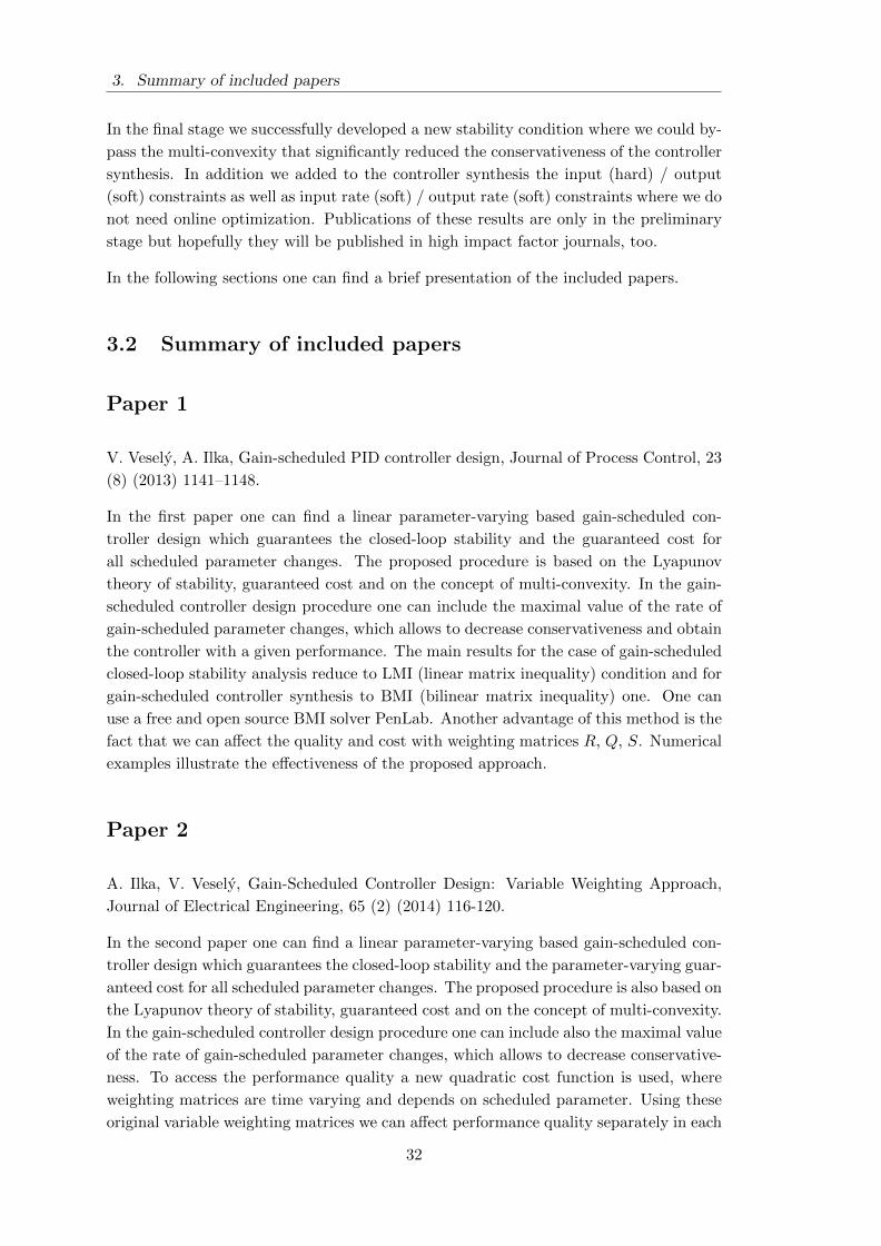
3. Summary of included papers
In the final stage we successfully developed a new stability condition where we could by-
pass the multi-convexity that significantly reduced the conservativeness of the controller
synthesis. In addition we added to the controller synthesis the input (hard) / output
(soft) constraints as well as input rate (soft) / output rate (soft) constraints where we do
not need online optimization. Publications of these results are only in the preliminary
stage but hopefully they will be published in high impact factor journals, too.
In the following sections one can find a brief presentation of the included papers.
3.2 Summary of included papers
Paper 1
V. Vesely, A. Ilka, Gain-scheduled PID controller design, Journal of Process Control, 23
(8) (2013) 1141–1148.
In the first paper one can find a linear parameter-varying based gain-scheduled con-
troller design which guarantees the closed-loop stability and the guaranteed cost for
all scheduled parameter changes. The proposed procedure is based on the Lyapunov
theory of stability, guaranteed cost and on the concept of multi-convexity. In the gain-
scheduled controller design procedure one can include the maximal value of the rate of
gain-scheduled parameter changes, which allows to decrease conservativeness and obtain
the controller with a given performance. The main results for the case of gain-scheduled
closed-loop stability analysis reduce to LMI (linear matrix inequality) condition and for
gain-scheduled controller synthesis to BMI (bilinear matrix inequality) one. One can
use a free and open source BMI solver PenLab. Another advantage of this method is the
fact that we can affect the quality and cost with weighting matrices R, Q, S. Numerical
examples illustrate the effectiveness of the proposed approach.
Paper 2
A. Ilka, V. Vesely, Gain-Scheduled Controller Design: Variable Weighting Approach,
Journal of Electrical Engineering, 65 (2) (2014) 116-120.
In the second paper one can find a linear parameter-varying based gain-scheduled con-
troller design which guarantees the closed-loop stability and the parameter-varying guar-
anteed cost for all scheduled parameter changes. The proposed procedure is also based on
the Lyapunov theory of stability, guaranteed cost and on the concept of multi-convexity.
In the gain-scheduled controller design procedure one can include also the maximal value
of the rate of gain-scheduled parameter changes, which allows to decrease conservative-
ness. To access the performance quality a new quadratic cost function is used, where
weighting matrices are time varying and depends on scheduled parameter. Using these
original variable weighting matrices we can affect performance quality separately in each
32
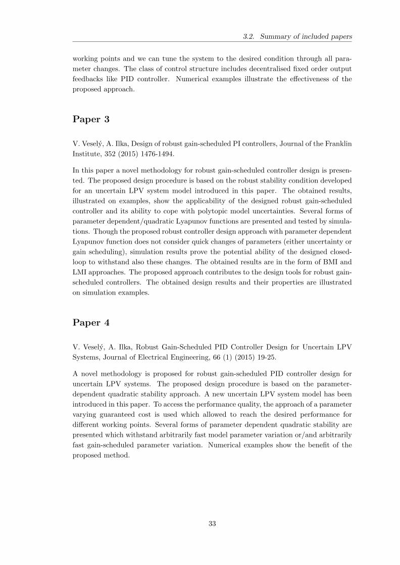
3.2. Summary of included papers
working points and we can tune the system to the desired condition through all para-
meter changes. The class of control structure includes decentralised fixed order output
feedbacks like PID controller. Numerical examples illustrate the effectiveness of the
proposed approach.
Paper 3
V. Vesely, A. Ilka, Design of robust gain-scheduled PI controllers, Journal of the Franklin
Institute, 352 (2015) 1476-1494.
In this paper a novel methodology for robust gain-scheduled controller design is presen-
ted. The proposed design procedure is based on the robust stability condition developed
for an uncertain LPV system model introduced in this paper. The obtained results,
illustrated on examples, show the applicability of the designed robust gain-scheduled
controller and its ability to cope with polytopic model uncertainties. Several forms of
parameter dependent/quadratic Lyapunov functions are presented and tested by simula-
tions. Though the proposed robust controller design approach with parameter dependent
Lyapunov function does not consider quick changes of parameters (either uncertainty or
gain scheduling), simulation results prove the potential ability of the designed closed-
loop to withstand also these changes. The obtained results are in the form of BMI and
LMI approaches. The proposed approach contributes to the design tools for robust gain-
scheduled controllers. The obtained design results and their properties are illustrated
on simulation examples.
Paper 4
V. Vesely, A. Ilka, Robust Gain-Scheduled PID Controller Design for Uncertain LPV
Systems, Journal of Electrical Engineering, 66 (1) (2015) 19-25.
A novel methodology is proposed for robust gain-scheduled PID controller design for
uncertain LPV systems. The proposed design procedure is based on the parameter-
dependent quadratic stability approach. A new uncertain LPV system model has been
introduced in this paper. To access the performance quality, the approach of a parameter
varying guaranteed cost is used which allowed to reach the desired performance for
different working points. Several forms of parameter dependent quadratic stability are
presented which withstand arbitrarily fast model parameter variation or/and arbitrarily
fast gain-scheduled parameter variation. Numerical examples show the benefit of the
proposed method.
33
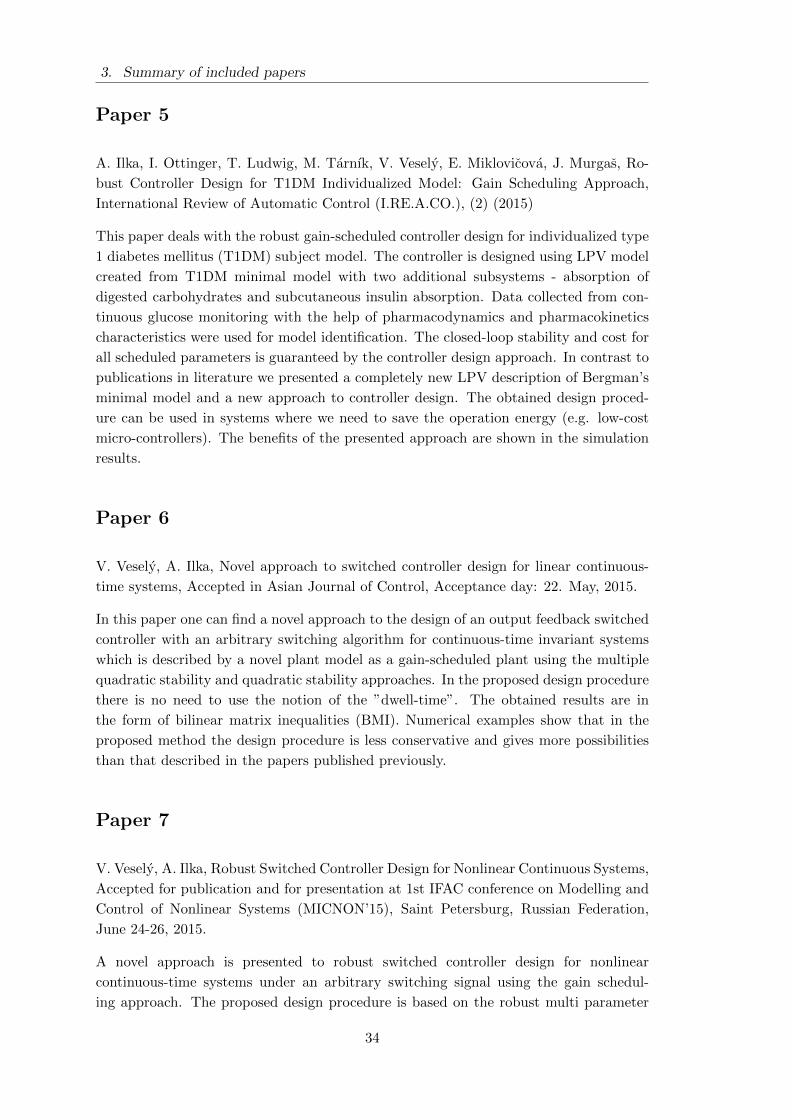
3. Summary of included papers
Paper 5
A. Ilka, I. Ottinger, T. Ludwig, M. Tarnık, V. Vesely, E. Miklovicova, J. Murgas, Ro-
bust Controller Design for T1DM Individualized Model: Gain Scheduling Approach,
International Review of Automatic Control (I.RE.A.CO.), (2) (2015)
This paper deals with the robust gain-scheduled controller design for individualized type
1 diabetes mellitus (T1DM) subject model. The controller is designed using LPV model
created from T1DM minimal model with two additional subsystems - absorption of
digested carbohydrates and subcutaneous insulin absorption. Data collected from con-
tinuous glucose monitoring with the help of pharmacodynamics and pharmacokinetics
characteristics were used for model identification. The closed-loop stability and cost for
all scheduled parameters is guaranteed by the controller design approach. In contrast to
publications in literature we presented a completely new LPV description of Bergman’s
minimal model and a new approach to controller design. The obtained design proced-
ure can be used in systems where we need to save the operation energy (e.g. low-cost
micro-controllers). The benefits of the presented approach are shown in the simulation
results.
Paper 6
V. Vesely, A. Ilka, Novel approach to switched controller design for linear continuous-
time systems, Accepted in Asian Journal of Control, Acceptance day: 22. May, 2015.
In this paper one can find a novel approach to the design of an output feedback switched
controller with an arbitrary switching algorithm for continuous-time invariant systems
which is described by a novel plant model as a gain-scheduled plant using the multiple
quadratic stability and quadratic stability approaches. In the proposed design procedure
there is no need to use the notion of the ”dwell-time”. The obtained results are in
the form of bilinear matrix inequalities (BMI). Numerical examples show that in the
proposed method the design procedure is less conservative and gives more possibilities
than that described in the papers published previously.
Paper 7
V. Vesely, A. Ilka, Robust Switched Controller Design for Nonlinear Continuous Systems,
Accepted for publication and for presentation at 1st IFAC conference on Modelling and
Control of Nonlinear Systems (MICNON’15), Saint Petersburg, Russian Federation,
June 24-26, 2015.
A novel approach is presented to robust switched controller design for nonlinear
continuous-time systems under an arbitrary switching signal using the gain schedul-
ing approach. The proposed design procedure is based on the robust multi parameter
34
3.2. Summary of included papers
dependent quadratic stability condition. The obtained switched controller design pro-
cedure for nonlinear continuous-time systems is in the bilinear matrix inequality form
(BMI). The obtained results, illustrated on examples, show the applicability of the
designed switched robust gain-scheduled controller and its ability to cope with model
uncertainties. In the paper several forms of parameter dependent/quadratic Lyapunov
functions are proposed. The properties of the obtained design are illustrated on simula-
tion examples.
Paper 8
A. Ilka, V. Vesely, Gain-Scheduled MPC Design for Nonlinear Systems with Input Con-
straints, Accepted for publication and for presentation at 1st IFAC conference on Mod-
elling and Control of Nonlinear Systems (MICNON’15), Saint Petersburg, Russian Fed-
eration, June 24-26, 2015.
A novel methodology is proposed for discrete model predictive gain-scheduled controller
design for nonlinear systems with input(hard)/output(soft) constraints for finite and
infinite prediction horizons. The proposed design procedure is based on the linear
parameter-varying (LPV) paradigm, affine parameter-dependent quadratic stability and
on the notion of the parameter-varying guaranteed cost. The design procedure is in the
form of BMI (we can use a free and open source BMI solver). Numerical examples show
the benefits for the finite and infinite prediction horizon.
Paper 9
V. Vesely, A. Ilka, Unified Robust Gain-Scheduled and Switched Controller Linear
Continuous-Time Systems, Submitted to International Review of Automatic Control
(I.RE.A.CO), Submitted on 25. May, 2015.
The proposed paper addresses the problem how to obtain the new unified procedure
to design a robust gain-scheduled and switched controller with arbitrary switching for
continuous-time systems described by a novel robust plant model using the parameter
dependent quadratic stability (PDQS) approach. The obtained unified controller design
procedure ensures the closed-loop stability and guaranteed cost for a prescribed rate of
change of the system switching (gain-scheduled) variable. In some real cases the rate of
change of the switching signal is finite. This assumption was used in the paper to obtain
the switched controller design procedure. Numerical examples illustrate the effectiveness
of the proposed approach.
35

4
Gain-scheduled PID controller design
(Paper 1)
Abstract
Gain scheduling (GS) is one of the most popular approaches to nonlinear control design
and it is known that GS controllers have a better performance than robust ones. Follow-
ing the terminology of control engineering, linear parameter-varying (LPV) systems are
time-varying plants whose state space matrices are fixed functions of some vector of vary-
ing parameters. Our approach is based on considering that the LPV system, scheduling
parameters and their derivatives with respect to time lie in a priori given hyper rect-
angles. To guarantee the performance we use the notion of guaranteed costs. The class
of control structure includes centralized, decentralized fixed order output feedbacks like
PID controller. Numerical examples illustrate the effectiveness of the proposed approach.
Keywords: Gain-scheduled control, controller design, structured controller, decentral-
ized control, MIMO LPV systems.
4.1 Introduction
Linear parameter-varying systems are time-varying plants whose state space matrices
are fixed functions of some vector of varying parameters θ(t). Linear parameter varying
(LPV) systems have the following interpretations:
– they can be viewed as linear time invariant (LTI) plants subject to time-varying
known parameters θ(t) ∈ 〈θ θ〉,
– they can be models of linear time-varying plants,
– they can be LTI plant models resulting from linearization of the nonlinear plants
along trajectories of the parameter θ(t) ∈ 〈θ θ〉 which can be measured.
37
Gain-scheduled PID controller design (Paper 1)
For the first and third class of systems, parameter θ can be exploited for the control
strategy to increase the performance of closed-loop systems. Hence, in this paper the
following LPV system will be used:
x = A(θ(t))x+B(θ(t))u
y = Cx(4.1)
where for the affine case
A(θ(t)) = A0 +A1θ1(t) + . . .+Apθp(t) (4.2)
B(θ(t)) = B0 +B1θ1(t) + . . .+Bpθp(t) (4.3)
and x ∈ Rn is the state, u ∈ Rm is a control input, y ∈ Rl is the measurement output
vector, A0, B0, Ai, Bi, i = 1, 2 . . . p, C are constant matrices of appropriate dimension,
θ(t) ∈ 〈θ θ〉 ∈ Ω and θ(t) ∈ 〈θ θ〉 ∈ Ωt are vectors of time-varying plant parameters
which belong to the known boundaries.
In the case of nonlinear dynamics a widely used idea among control engineers is to
linearize the plant around several operating points and to use linear control tools to
design a controller for each of these points. The actual controller is implemented using
the gain scheduling approach. Success of such an approach depends on establishing the
relationship between a nonlinear system and a family of linear ones. There are two main
problems:
1. Stability results: stability of the closed-loop nonlinear system and of the closed-
loop family of linear systems, when scheduled parameters are changes.
2. Approximation results which provide a direct relationship between the solution of
closed-loop nonlinear systems and the solution of associated linear systems [1], [2]
The main motivation for our work lies in [3], [4], [5], [6], [7], [8], where in [3] the LPV
controller is designed using the bounded real lemma for continuous and discrete time
LPV systems such as to guarantee H∞ performance.
Paper [4] discusses extensions of H∞ synthesis techniques to allow for controller depend-
ence on time-varying but measured parameters. In this case a higher performance can
be achieved by control laws that incorporate measurements of θ to the control algorithm.
Main results can be formulated as follows: Find a control structure such that the LPV
controller satisfies closed-loop stability and minimizes of the induced L2 norm of corres-
ponding closed-loop systems. The author’s approach [5] uses a bounding technique based
on parameter-dependent Lyapunov function for design of PD controllers. Note that if
LPV synthesis problem is solvable, then the induced L2-norm of the closed-loop system
is less than some given constant. The proposed approach represents generalization of
the standard sub-optimal H∞ control problem. In paper [6] the author shows that the
performance of LPV systems with LPV controller can be improved by combining this
38
4.1. Introduction
LMI method with MPC techniques and optimizing the H2 (H∞) norm. The author [8]
tackles the design problem of gain scheduled controllers for LPV systems via parameter-
dependent Lyapunov function. The author proposed a new design method as a set LMIs
with single line search parameters. The author tackles two problems: H∞ type problem
and H2. Recently, [9] proposed the design method for the gain scheduled problem using
a similar technique to [8]. In the above paper the LPV controller is given in time domain
with the same or lower order than the LPV systems using H∞ optimization approach.
The gain scheduling controller design for discrete-time systems is given in [10]. Paper
[11] presents the design of gain-scheduled PI controller, when the uncertainty of the sys-
tem is assumed to be the difference between the nonlinear model and the nominal linear
model. PI controller is designed using quadratic Lyapunov H∞ performance where index
γ is H∞ norm of closed-loop system, considered as closed-loop performance measure.
Minimizing γ via LMI the gain scheduled controller is obtained. In [12] the authors
design a novel gain scheduling controller for synchronous generator. Improved stability
analysis and gain scheduled controller synthesis for parameter-dependent systems are
proposed in [7]. Sufficient conditions for robust stability as well as conditions for the
existence of a gain-scheduled controller are given in terms of a set of LMIs. The author’s
approach is based on the notion of quadratic stability and linear fractional representa-
tion for parameter dependent systems. The survey of scheduled controller analysis and
synthesis can be found in excellent papers [1] and [2].
In this paper our approach is based on:
– A consideration of the LPV systems (4.1). The scheduling parameters θi, i =
1, 2, . . . p and their derivatives with respect to time are supposed to lie in a priori
given hyper rectangles.
– Affine quadratic stability (AQS) introduced by [13].
– To guarantee the performance we use the notion of guaranteed cost to optimize
the given cost function.
– The class of control structure includes centralized, decentralized fixed order output
feedback like PID controller.
The gain-scheduled controller design procedure is in the form of BMI. A feasible solution
for closed-loop system ensures the affine quadratic stability [13] and guaranteed cost
when the performance is defined in Q,R, S structure (see eq. (4.10)).
Quadratic stability (one Lyapunov function with one constant positive definite matrix
cover all affine controller design procedure) is more conservative than AQS in general.
AQS (Lyapunov function has an affine structure like (4.2)) incorporates information
about the rate of variation θ(t) to reduce conservatism. As we mentioned, in this paper
the AQS approach will be used.
Our notations are standard. D ∈ Rm×n denotes the set of real m×n matrices. Im is an
m×m identity matrix. If the size can be determined from the context, we will omit the
subscript. P > 0 (P ≥ 0) is a real symmetric, positive definite (semi-definite) matrix.
39
Gain-scheduled PID controller design (Paper 1)
The paper is organized as follows. Section 4.2 brings preliminaries and problem formu-
lation. The main result is presented in Section 4.3. In Section 4.4, numerical examples
illustrate the effectiveness of the proposed approach.
4.2 Preliminaries and problem formulation
Suppose that the state-space representation of an LPV system with p independent
scheduling parameters is governed by (4.1). The scheduling parameters θi and their
derivatives with respect to time θi are supposed to lie in given hyper rectangles Ω and
Ωt, respectively. For design of the I part of the controller system, equation (4.1) has
to be augmented, see [14] and example 1. Without change of notation the new aug-
mented matrices dimensions are A(θ) ∈ R(n+l)×(n+l), B(θ) ∈ R(n+l)×m, C ∈ R2l×2l
and Cd ∈ Rl×l is the output matrix for D part of controller. The output feedback
gain-scheduled control law is considered for PID controller in the form
u(t) = F (θ)y + Fd(θ)yd = F (θ)Cx+ FdCdx (4.4)
where yd = Cdx is the output feedback for the D part of the controller,
F (θ) = F0 +
p∑i=1
Fiθi ∈ Rm×2l (4.5)
is the static output feedback gain scheduled matrix for the PI controller and
Fd(θ) = Fd0 +
p∑i=1
Fdiθi ∈ Rm×m (4.6)
is the static output feedback gain scheduled matrix for the D part of controller.
Remark 4.1. Since the reference signal does not influence the closed-loop stability, we
assume that it is equal to zero.
Remark 4.2. If the derivative part of the controller includes some filter, the model of
this filter can be included in the system model.
The closed-loop system is then
[I −B(θ)Fd(θ)Cd]x = [A(θ) +B(θ)F (θ)C]x (4.7)
Ad(θ)x = Ac(θ)x (4.8)
x = Acd(θ)x (4.9)
where
Acd(θ) = Ad(θ)−1Ac(θ)x
Ad(θ) = I −B(θ)Fd(θ)Cd
Ac(θ) = A(θ) +B(θ)F (θ)C
40
4.3. Main results
It is well known that the fixed order dynamic output feedback control design problem is
a special case of the static output feedback problem. To access the performance quality
a quadratic cost function [15] known from LQ theory is often used in the form
J =
∫ ∞0
(xTQx+ uTRu+ xTSx)dt (4.10)
with Q = QT ≥ 0, R > 0 and S = ST ≥ 0. The guaranteed cost is defined in a standard
way.
Definition 4.1. Consider system (4.1) with control algorithm (4.4). If there exists a
control law u∗ and a positive scalar J∗ such that the closed-loop system (4.7) is stable
and the value of closed-loop cost function (4.10) satisfies J ≤ J∗, then J∗ is said to be
a guaranteed cost and u∗ is said to be guaranteed cost control law for system (4.1).
Definition 4.2. [13] The linear closed-loop system (4.7) for θ ∈ Ω and θ ∈ Ωt is affinely
quadratically stable if and only if there exist p + 1 symmetric matrices P0, P1, . . . , Ppsuch that
P (θ) = P0 +
p∑i=1
Piθi > 0 (4.11)
and for the first derivative of Lyapunov function V (θ) = xTP (θ)x along the trajectory
of closed-loop system (4.7) it holds
dV (x, θ)
dt= xT
(Acd(θ)
TP (θ) + P (θ)Acd(θ) +dP (θ)
dt
)x < 0 (4.12)
where
dP (θ)
dt=
p∑i=1
Piθi ≤p∑i=1
Piρi
From LQ theory we introduce the well known results.
Lemma 4.1. Consider the closed-loop system (4.7). Closed-loop system (4.7) is affinely
quadratically stable with guaranteed cost if and only if the following inequality holds
Be = minu
dV (θ)
dt+ xTQx+ uTRu+ xTSx
≤ 0 (4.13)
for all θ ∈ Ω and θ ∈ Ωt
4.3 Main results
In this section the gain scheduled controller design procedure which guarantees the
affine quadratic stability and guaranteed cost for θ ∈ Ω and θ ∈ Ωt is presented. The
41
Gain-scheduled PID controller design (Paper 1)
main results for the case of gain scheduled closed-loop stability analysis reduce to LMI
condition and for gain scheduled controller synthesis to BMI one.
The main result of this section, the gain scheduled design procedure, relies in the concept
of multi-convexity, that is, convexity along each direction θi of the parameter space. The
implications of multiconvexity for scalar quadratic functions are given in the next lemma
[13].
Lemma 4.2. Consider a scalar quadratic function of θ ∈ Rp.
f (θ1, . . . , θp) = a0 +
p∑i=1
aiθi +
p∑i,j=1
bijθiθj +
p∑i=1
ciθ2i (4.14)
and assume that f (θ1, . . . , θp) is multi-convex, that is
∂2f(θ)
∂θ2i
= 2ci ≥ 0 (4.15)
for i = 1, 2, . . . , p. Then f(θ) is negative for all θ ∈ Ω if and only if it takes negative
values at the corners of θ.
Using Lemma 4.2 the following theorem is obtained
Theorem 4.1. Closed-loop system (4.7) is AQS with guaranteed cost if there exist p+
1 definite matrices P0, P1, P2, . . . , Pp such that P (θ) (4.11) is positive defined for all
θ ∈ Ω, matrices N1, N2, Q,R, S and controller gain scheduled matrices F (θ) and Fd(θ),
satisfying
M(θ) < 0; θ ∈ Ω (4.16a)
Mii ≥ 0; i = 1, 2, . . . , p (4.16b)
where
M(θ) = M0 +
p∑i=1
Miθi +
p∑i=1
p∑j=1
Mijθiθj
M0 =
[W110 W120
W120T W220
]
Mi =
[W11i W12i
W12iT W22i
]
Mij =
[W11ij W12ij
W12ijT W22ij
]
42
4.3. Main results
W110 = N1Ad0 +AdT0 N
T1 + CTd Fd
T0 RFd0Cd + S
W11i = N1Adi +AdTi N
T1 + CTd Fd
T0 RFdiCd
+ CTd FdTi RFd0Cd
W11ij = N1Adij +AdTijN
T1 + CTd Fd
Ti RFdjCd
W120 = P0 +AdT0 N
T2 −N1Ac0 + CTd Fd
Ti RF0C
W12i = Pi +AdTi N
T2 −N1Aci + CTd Fd
T0 RFiC
+ CTd FdTi RF0C
W12ij = AdTijN
T2 −N1Acij + CTd Fd
Ti RFjC
W220 =
p∑k=1
Pkρk −N2Ac0 −AcT0 NT2 +Q
+ CTF T0 RF0C; ρk ∈ Ωt
W22i = −N2Aci −AcTi NT2 + CTF T0 RFiC
+ CTF Ti RF0C
W22ij = −N2Acij −AcTijNT2 + CTF Ti RFjC
Ac0 = A0 +B0F0C
Aci = Ai +B0FiC +BiF0C
Acij = BiFjC
Ad0 = I −B0Fd0Cd
Adi = −B0FdiCd −BiFd0Cd
Adij = −BiFdjCd
Proof. Proof is based on Lemmas 4.1 and 4.2. From (4.8) and (4.12) we can obtain
[2N1x+ 2N2x]T [Ad(θ)x−Ac(θ)x] = 0 (4.17)
and
dV
dt= xTP (θ)x+ xTP (θ)x+ xT P (θ)x (4.18)
Summarizing the above two equations, for the time derivative of Lyapunov function one
obtains
dV
dt= zT
[N1Ad(θ) +Ad(θ)
TNT1 −N1Ac(θ) +ATdN
T2 + P (θ)
∗ −N2Ac(θ)−ATc (θ)NT2 +
∑pi=1 Piρi
]z (4.19)
where N1, N2 ∈ Rn×n are auxiliary matrices and zT =[xT xT
]. When one sub-
stitutes control algorithm (4.4) to the right hand side of (4.13) and then the obtained
result is combined with (4.19) and substituted to (4.13), after some manipulation, using
Lemma 4.2 we obtain (4.16), which proofs the Theorem 4.1.
43
Gain-scheduled PID controller design (Paper 1)
Let us denote θm =∑p
i=1 θi, multiplying (4.16a) with∑p
i=1θiθm
assuming that θm 6= 0
and θm ∈ 〈θm, θm〉 we obtain
M0
θ2m
p∑i=1
p∑j=1
θiθj +
p∑i=1
p∑j=1
Mi
θmθiθj +
p∑i=1
p∑j=1
Mijθiθj < 0 (4.20)
After small manipulation
p∑i=1
p∑j=1
[M0 +Miθm +Mijθ
2m
]θiθj < 0 (4.21)
The closed-loop system will be stable or (4.21) holds if
Kij +Kji < 0, i = 1, 2, . . . , p, j = i, i+ 1, . . . , p (4.22)
where
Kij = M0 +Miθm +Mijθ2m
Using stability conditions (4.22) and Lemma 4.2 if the following inequalities are met,
the closed-loop system is affine quadratically stable
2M0 + (Mi +Mj) θm + (Mij +Mji) θ2m < 0
2M0 + (Mi +Mj) θm + (Mij +Mji) θ2m < 0
Mij +Mji ≥ 0
(4.23)
for i = 1, 2, . . . , p, j = i, i+ 1, . . . , p.
Lemma 4.3. Closed-loop system (4.7) is AQS with guaranteed cost if there exist p+ 1
definite matrices P0, P1, . . . , Pp such that for all θ ∈ Ω, P (θ) (4.11) is positive definite,
matrices N1, N2 and gain scheduled matrices F (θ) and Fd(θ) are satisfying (4.23).
If the solution of Theorem 4.1 or Lemma 4.3 are feasible:
– For the case of closed-loop system stability, with respect to matrices N1, N2 and
positive definite matrix P (θ) the closed-loop system is affine quadratically stable
with guaranteed cost and for θ ∈ Ω, θ ∈ Ωt. For this case gain matrices (4.4), (4.5)
and (4.6) are known and (4.16), (4.23) reduces to LMI.
– For the gain-scheduled controller design with respect to matrices F (θ), Fd(θ), N1,
N2 and positive definite matrix P (θ), the closed-loop system is affine quadratically
stable with guaranteed cost and for θ ∈ Ω, θ ∈ Ωt. For this case (4.16) and (4.23)
are BMI.
44
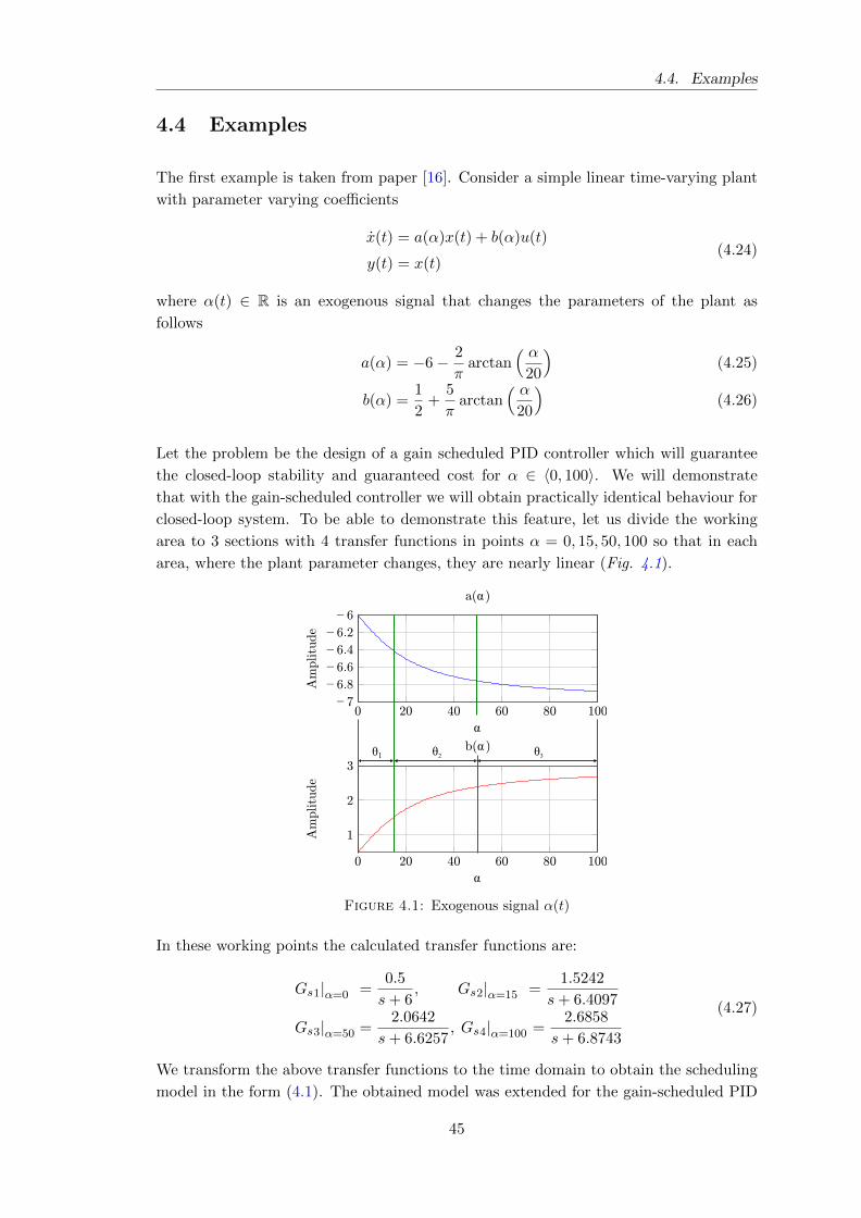
4.4. Examples
4.4 Examples
The first example is taken from paper [16]. Consider a simple linear time-varying plant
with parameter varying coefficients
x(t) = a(α)x(t) + b(α)u(t)
y(t) = x(t)(4.24)
where α(t) ∈ R is an exogenous signal that changes the parameters of the plant as
follows
a(α) = −6− 2
πarctan
( α20
)(4.25)
b(α) =1
2+
5
πarctan
( α20
)(4.26)
Let the problem be the design of a gain scheduled PID controller which will guarantee
the closed-loop stability and guaranteed cost for α ∈ 〈0, 100〉. We will demonstrate
that with the gain-scheduled controller we will obtain practically identical behaviour for
closed-loop system. To be able to demonstrate this feature, let us divide the working
area to 3 sections with 4 transfer functions in points α = 0, 15, 50, 100 so that in each
area, where the plant parameter changes, they are nearly linear (Fig. 4.1).
0 20 40 60 80 100− 7
− 6 8
− 6 6
− 6 4
− 6 2
− 6
α
Amplitude
a(α )
0 20 40 60 80 100
1
2
3
α
Amplitude
b(α )θ1 θ
2θ3
Figure 4.1: Exogenous signal α(t)
In these working points the calculated transfer functions are:
Gs1|α=0 =0.5
s+ 6, Gs2|α=15 =
1.5242
s+ 6.4097
Gs3|α=50 =2.0642
s+ 6.6257, Gs4|α=100 =
2.6858
s+ 6.8743
(4.27)
We transform the above transfer functions to the time domain to obtain the scheduling
model in the form (4.1). The obtained model was extended for the gain-scheduled PID
45
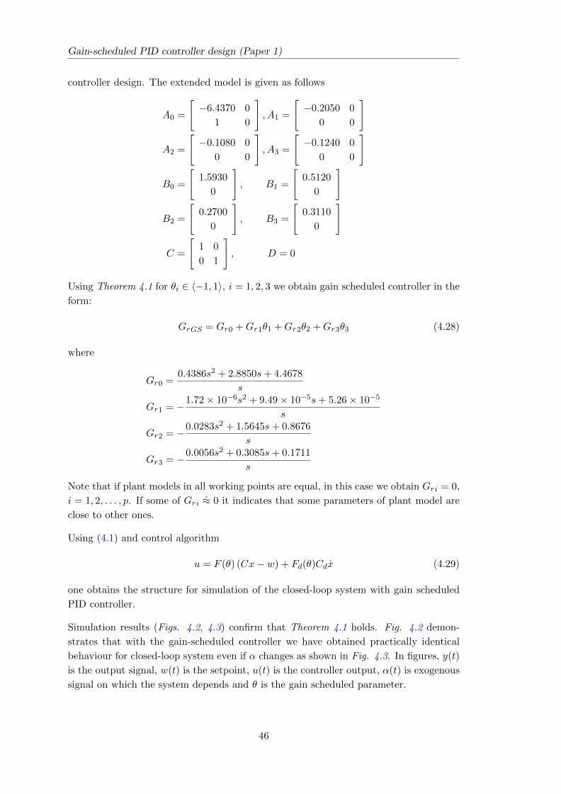
Gain-scheduled PID controller design (Paper 1)
controller design. The extended model is given as follows
A0 =
[−6.4370 0
1 0
], A1 =
[−0.2050 0
0 0
]
A2 =
[−0.1080 0
0 0
], A3 =
[−0.1240 0
0 0
]
B0 =
[1.5930
0
], B1 =
[0.5120
0
]
B2 =
[0.2700
0
], B3 =
[0.3110
0
]
C =
[1 0
0 1
], D = 0
Using Theorem 4.1 for θi ∈ 〈−1, 1〉, i = 1, 2, 3 we obtain gain scheduled controller in the
form:
GrGS = Gr0 +Gr1θ1 +Gr2θ2 +Gr3θ3 (4.28)
where
Gr0 =0.4386s2 + 2.8850s+ 4.4678
s
Gr1 = −1.72× 10⁻⁶s2 + 9.49× 10⁻⁵s+ 5.26× 10⁻⁵
s
Gr2 = −0.0283s2 + 1.5645s+ 0.8676
s
Gr3 = −0.0056s2 + 0.3085s+ 0.1711
s
Note that if plant models in all working points are equal, in this case we obtain Gri = 0,
i = 1, 2, . . . , p. If some of Gri ≈ 0 it indicates that some parameters of plant model are
close to other ones.
Using (4.1) and control algorithm
u = F (θ) (Cx− w) + Fd(θ)Cdx (4.29)
one obtains the structure for simulation of the closed-loop system with gain scheduled
PID controller.
Simulation results (Figs. 4.2, 4.3) confirm that Theorem 4.1 holds. Fig. 4.2 demon-
strates that with the gain-scheduled controller we have obtained practically identical
behaviour for closed-loop system even if α changes as shown in Fig. 4.3. In figures, y(t)
is the output signal, w(t) is the setpoint, u(t) is the controller output, α(t) is exogenous
signal on which the system depends and θ is the gain scheduled parameter.
46
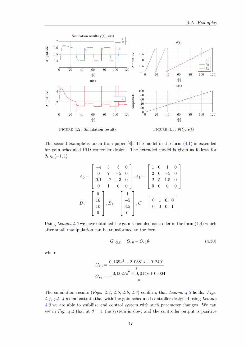
4.4. Examples
0 20 40 60 80 100 120
0.4
0.5
0.6
0.7
t[s]
Amplitude
Simulation results y(t), w(t)yw
0 20 40 60 80 100 120
2
4
t[s]
Amplitude
u(t)
u
Figure 4.2: Simulation results
0 20 40 60 80 100 120−1
−0.5
0
0.5
1
t[s]
Amplitude
θ(t)
θ1θ2θ3
0 20 40 60 80 100 1200
20
40
60
80
100
t[s]
Amplitude
α(t)
Figure 4.3: θ(t), α(t)
The second example is taken from paper [8]. The model in the form (4.1) is extended
for gain scheduled PID controller design. The extended model is given as follows for
θ1 ∈ 〈−1, 1〉
A0 =
−4 3 5 0
0 7 −5 0
0.1 −2 −3 0
0 1 0 0
, A1 =
1 0 1 0
2 0 −5 0
2 5 1.5 0
0 0 0 0
B0 =
0
16
10
0
, B1 =
1
−5
3.5
0
, C =
[0 1 0 0
0 0 0 1
]
Using Lemma 4.3 we have obtained the gain-scheduled controller in the form (4.4) which
after small manipulation can be transformed to the form
GrGS = Gr0 +Gr1θ1 (4.30)
where
Gr0 =0, 139s2 + 2, 0381s+ 0, 2401
s
Gr1 = −0, 0027s2 + 0, 014s+ 0, 004
s
The simulation results (Figs. 4.4, 4.5, 4.6, 4.7) confirm, that Lemma 4.3 holds. Figs.
4.4, 4.5, 4.6 demonstrate that with the gain-scheduled controller designed using Lemma
4.3 we are able to stabilize and control system with such parameter changes. We can
see in Fig. 4.4 that at θ = 1 the system is slow, and the controller output is positive
47
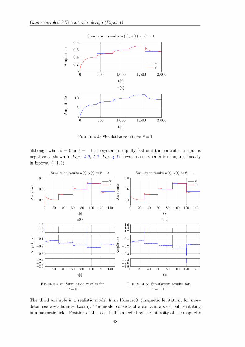
Gain-scheduled PID controller design (Paper 1)
0 500 1,000 1,500 2,0000
0.2
0.4
0.6
0.8
t[s]
Amplitude
Simulation results w(t), y(t) at θ = 1
wy
0 500 1,000 1,500 2,0000
5
10
t[s]
Amplitude
u(t)
Figure 4.4: Simulation results for θ = 1
although when θ = 0 or θ = −1 the system is rapidly fast and the controller output is
negative as shown in Figs. 4.5, 4.6. Fig. 4.7 shows a case, when θ is changing linearly
in interval 〈−1, 1〉.
0 20 40 60 80 100 120 140
0.4
0.6
0.8
t[s]
Amplitude
Simulation results w(t), y(t) at θ = 0
wy
1.21.41.6
u(t)
−0.3
−0.2
−0.1
Amplitude
0 20 40 60 80 100 120 140−2.8−2.6−2.4
t[s]
Figure 4.5: Simulation results forθ = 0
0 20 40 60 80 100 120 140
0.4
0.6
0.8
t[s]
Amplitude
Simulation results w(t), y(t) at θ = -1
wy
1.21.41.6
u(t)
−0.3
−0.2
−0.1
Amplitude
0 20 40 60 80 100 120 140−2.8−2.6−2.4
t[s]
Figure 4.6: Simulation results forθ = −1
The third example is a realistic model from Humusoft (magnetic levitation, for more
detail see www.humusoft.com). The model consists of a coil and a steel ball levitating
in a magnetic field. Position of the steel ball is affected by the intensity of the magnetic
48
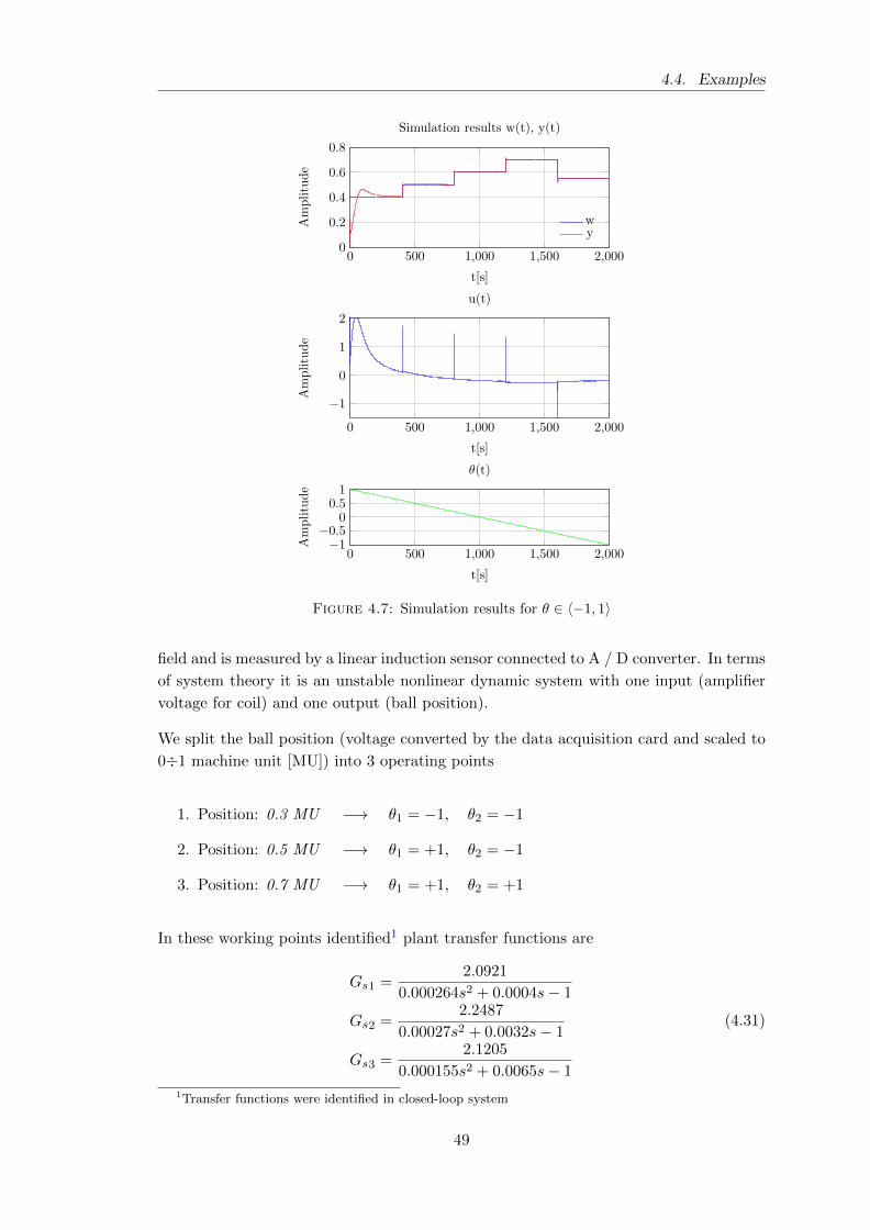
4.4. Examples
0 500 1,000 1,500 2,000
−1
0
1
2
t[s]
Amplitude
u(t)
0 500 1,000 1,500 2,0000
0.2
0.4
0.6
0.8
t[s]
Amplitude
Simulation results w(t), y(t)
wy
0 500 1,000 1,500 2,000−1
−0.50
0.51
t[s]
Amplitude
θ(t)
Figure 4.7: Simulation results for θ ∈ 〈−1, 1〉
field and is measured by a linear induction sensor connected to A / D converter. In terms
of system theory it is an unstable nonlinear dynamic system with one input (amplifier
voltage for coil) and one output (ball position).
We split the ball position (voltage converted by the data acquisition card and scaled to
0÷1 machine unit [MU]) into 3 operating points
1. Position: 0.3 MU −→ θ1 = −1, θ2 = −1
2. Position: 0.5 MU −→ θ1 = +1, θ2 = −1
3. Position: 0.7 MU −→ θ1 = +1, θ2 = +1
In these working points identified1 plant transfer functions are
Gs1 =2.0921
0.000264s2 + 0.0004s− 1
Gs2 =2.2487
0.00027s2 + 0.0032s− 1
Gs3 =2.1205
0.000155s2 + 0.0065s− 1
(4.31)
1Transfer functions were identified in closed-loop system
49
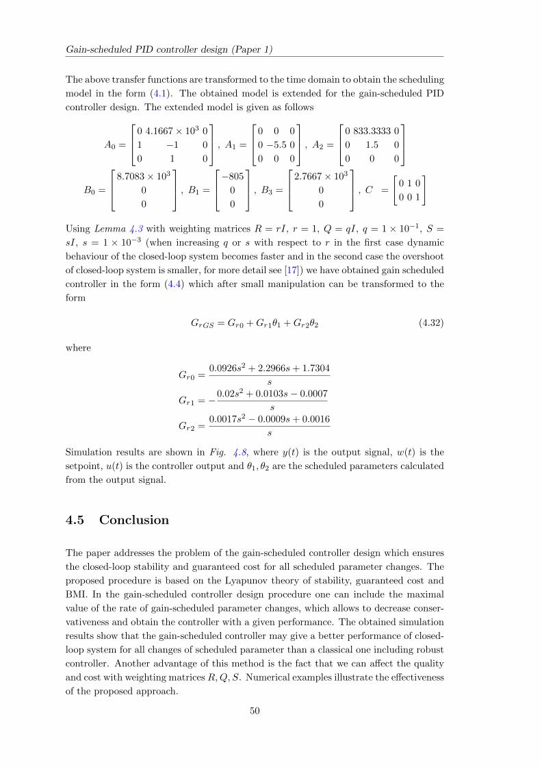
Gain-scheduled PID controller design (Paper 1)
The above transfer functions are transformed to the time domain to obtain the scheduling
model in the form (4.1). The obtained model is extended for the gain-scheduled PID
controller design. The extended model is given as follows
A0 =
0 4.1667× 10³ 0
1 −1 0
0 1 0
, A1 =
0 0 0
0 −5.5 0
0 0 0
, A2 =
0 833.3333 0
0 1.5 0
0 0 0
B0 =
8.7083× 10³
0
0
, B1 =
−805
0
0
, B3 =
2.7667× 10³
0
0
, C =
[0 1 0
0 0 1
]
Using Lemma 4.3 with weighting matrices R = rI, r = 1, Q = qI, q = 1 × 10⁻¹, S =
sI, s = 1 × 10⁻³ (when increasing q or s with respect to r in the first case dynamic
behaviour of the closed-loop system becomes faster and in the second case the overshoot
of closed-loop system is smaller, for more detail see [17]) we have obtained gain scheduled
controller in the form (4.4) which after small manipulation can be transformed to the
form
GrGS = Gr0 +Gr1θ1 +Gr2θ2 (4.32)
where
Gr0 =0.0926s2 + 2.2966s+ 1.7304
s
Gr1 = −0.02s2 + 0.0103s− 0.0007
s
Gr2 =0.0017s2 − 0.0009s+ 0.0016
s
Simulation results are shown in Fig. 4.8, where y(t) is the output signal, w(t) is the
setpoint, u(t) is the controller output and θ1, θ2 are the scheduled parameters calculated
from the output signal.
4.5 Conclusion
The paper addresses the problem of the gain-scheduled controller design which ensures
the closed-loop stability and guaranteed cost for all scheduled parameter changes. The
proposed procedure is based on the Lyapunov theory of stability, guaranteed cost and
BMI. In the gain-scheduled controller design procedure one can include the maximal
value of the rate of gain-scheduled parameter changes, which allows to decrease conser-
vativeness and obtain the controller with a given performance. The obtained simulation
results show that the gain-scheduled controller may give a better performance of closed-
loop system for all changes of scheduled parameter than a classical one including robust
controller. Another advantage of this method is the fact that we can affect the quality
and cost with weighting matrices R,Q, S. Numerical examples illustrate the effectiveness
of the proposed approach.
50
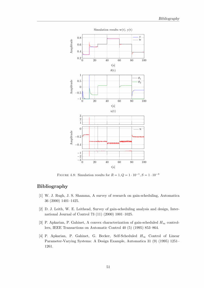
Bibliography
0 20 40 60 80 1000.2
0.4
0.6
0.8
t[s]
Amplitude
Simulation results w(t), y(t)
yw
0 20 40 60 80 100−1
−0.5
0
0.5
1
t[s]
Amplitude
θ(t)
θ1θ2
123
u(t)
−0.4
−0.2
0
Amplitude
u
0 20 40 60 80 100−3−2−1
t[s]
Figure 4.8: Simulation results for R = 1, Q = 1 · 10−1, S = 1 · 10−3
Bibliography
[1] W. J. Rugh, J. S. Shamma, A survey of research on gain-scheduling, Automatica
36 (2000) 1401–1425.
[2] D. J. Leith, W. E. Leithead, Survey of gain-scheduling analysis and design, Inter-
national Journal of Control 73 (11) (2000) 1001–1025.
[3] P. Apkarian, P. Gahinet, A convex characterization of gain-scheduled H∞ control-
lers, IEEE Transactions on Automatic Control 40 (5) (1995) 853–864.
[4] P. Apkarian, P. Gahinet, G. Becker, Self-Scheduled H∞ Control of Linear
Parameter-Varying Systems: A Design Example, Automatica 31 (9) (1995) 1251–
1261.
51
Gain-scheduled PID controller design (Paper 1)
[5] F. Wu, X. H. Yang, A. Packard, G. Becker, Induced L2-Norm Control for LPV
Systems with Bounded Parameter Variation Rates, International Journal of Robust
and Nonlinear Control 6 (1996) 2379–2383.
[6] M. Sznaier, Receding horizon: an easy way to improve performance in LPV systems,
in: Proceedings of the 1999 American Control Conference, Vol. 4, 1999, pp. 2257–
2261.
[7] F. Wang, V. Balakrishnan, Improved stability analysis and gain-scheduled control-
ler synthesis for parameter-dependent systems, IEEE Transactions on Automatic
Control 47 (5) (2002) 720–734.
[8] M. Sato, Brief paper: Gain-scheduled output-feedback controllers depending solely
on scheduling parameters via parameter-dependent Lyapunov functions, Automat-
ica 47 (12) (2011) 2786–2790.
[9] H. Koroglu, Robust generalized asymptotic regulation via an LPV controller
without parameter derivative dependence, in: 49th IEEE Conference on Decision
and Control (CDC), 2010, pp. 4965–4971.
[10] F. Adegas, J. Stoustrup, Structured control of affine linear parameter varying sys-
tems, in: American Control Conference (ACC), 2011, pp. 739–744.
[11] J. Gao, H. M. Budman, Design of robust gain-scheduled PI controllers for nonlinear
processes, Journal of Process Control 15 (7) (2005) 807–817.
[12] R. Mohammadi-Milasi, M. Yazdanpanah, P. Jabehdar-Maralani, A novel adaptive
gain-scheduling controller for synchronous generator, in: Proceedings of the 2004
IEEE International Conference on Control Applications, Vol. 1, 2004, pp. 800–805.
[13] P. Gahinet, P. Apkarian, M. Chilali, Affine parameter-dependent Lyapunov func-
tions and real parametric uncertainty, IEEE Transactions on Automatic Control
41 (3) (1996) 436–442.
[14] V. Vesely, D. Rosinova, Robust PID-PSD Controller Design: BMI approach, Assian
Journal of Control 15 (2) (2013) 469–478.
[15] J. Engwerda, A. Weeren, A result on output feedback linear quadratic control,
Automatica 44 (1) (2008) 265–271.
[16] G. E. Stewart, A Pragmatic Approach to Robust Gain Scheduling, in: 7th IFAC
Symposium on Robust Control Design, Vol. 7, Aalborg Congress & Culture Centre,
Denmark, 2012, pp. 355–362.
[17] M. Athans, P. Falb, Optimal control., McGraw-Hill Electrical and Electronik En-
gineering Series. Maidenhead, Berksh.: McGraw-Hill Publishing Company, Ltd. 879
p. New York, 1966.
52
5
Gain-Scheduled Controller Design:
Variable Weighting Approach (Paper 2)
Abstract
Among the most popular approaches to nonlinear control is gain-scheduled (GS) con-
troller, which can have better performance than robust and other ones. Our approach
is based on a consideration that in linear parameter varying (LPV) system, scheduling
parameters and their derivatives with respect to time are supposed to lie in a priori given
hyper rectangles. To access the performance quality a new quadratic cost function is
used, where weighting matrices are time varying depends on scheduled parameter. The
class of control structure includes decentralised fixed order output feedbacks like PID
controller. Numerical examples illustrate the effectiveness of the proposed approach.
Keywords: Gain-scheduled control, decentralised control, Lyapunov function, quad-
ratic cost function, MIMO LPV systems, PID controller.
5.1 Introduction
Consider a linear parameter varying (LPV) system with state space matrices which are
fixed functions of known vector parameter varying θ(t). This model can be a linear time
invariant (LTI) plant model which is result from linearisation of the nonlinear plants
along trajectories of the known parameter θ(t) ∈ 〈θ, θ〉. In this note the following LPV
system will be used
x = A(θ(t))x+B(θ(t))u
y = Cx(5.1)
53
Gain-Scheduled Controller Design: Variable Weighting Approach (Paper 2)
where
A(θ(t)) = A0 +A1θ1(t) + . . .+Apθp(t)
B(θ(t)) = B0 +B1θ1(t) + . . .+Bpθp(t)
and x ∈ Rn is the state, u ∈ Rm is a control input, y ∈ Rl is the measurement output
vector, A0, B0, Ai, Bi, i = 1, 2, . . . , p, C are constant matrices of appropriate dimension,
θ(t) ∈ 〈θ, θ〉 ∈ Ω vector of time-varying plant parameters.
The main motivation for our work lies in [1–5]. In the paper [1] the author tackles the
design problem of gain scheduled controllers for LPV systems via parameter-dependent
Lyapunov function. Recently, [2] proposed the design method for gain scheduled problem
using a similar technique to [1]. Improved stability analysis and gain scheduled controller
synthesis for parameter-dependent systems are proposed in [3]. Survey of scheduled
controller analysis and synthesis are presented in papers [4] and [5].
In this note our approach is based on
• A consideration of the LPV systems (5.1), scheduling parameters θi, i = 1, 2, . . . , p
and their derivatives with respect to time are supposed to lie in a priori given
hyper rectangles, θ ∈ Ω and θ ∈ Ωt.
• Affine quadratic stability (AQS) introduced by [6].
• We use the notion of guaranteed cost to guarantee the performance of closed-loop
system.
• The class of control structure includes decentralised fixed order output feedback
like PID controller.
The paper is organised as follows. Section 5.2 brings preliminaries and problem formu-
lation. The main result is presented in Section 5.3. In Section 5.4, numerical example
illustrate the effectiveness of the proposed approach.
5.2 Preliminaries and Problem Formulation
Consider an LPV system with p independent scheduling parameters in the form (5.1).
The output feedback control law is considered for PID controller in the form
u(t) = F (θ)y + Fd(θ)y = F (θ)Cx+ FdCdx (5.2)
where
F (θ) = F0 +
p∑i=1
Fiθi
54
5.2. Preliminaries and Problem Formulation
is a static output feedback gain scheduled matrix for PI controller and
Fd(θ) = Fd0 +
p∑i=1
Fdiθi
is a static output feedback gain scheduled matrix for D part of controller. Substituting
(5.2) to (5.1) and after some manipulation we can obtain the closed-loop system in the
following form
Ad(θ)x = Ac(θ)x (5.3)
where
Ad(θ) = I −B(θ)Fd(θ)Cd
Ac(θ) = A(θ) +B(θ)F (θ)C
To access the performance quality a quadratic cost function [7] known from LQ theory
is often used. In this note the original quadratic cost function is used, where weighting
matrices depends on scheduling parameters. Using this approach we can affect on per-
formance quality in each working point separately. The quadratic cost function is in the
form
J(θ) =
∫ ∞0
(xTQ(θ)x+ uTRu+ xTS(θ)x
)dt (5.4)
where
Q(θ) = Q0 +
p∑i=1
Qiθi, Qi = QTi ≥ 0
S(θ) = S0 +
p∑i=1
Siθi, Si = STi ≥ 0
and R > 0. The guaranteed cost is defined in a standard way.
Definition 5.1. Consider the system (5.1) with control algorithm (5.2). If there exists
a control law u∗ and a positive scalar J∗ such that the closed-loop system (5.3) is stable
and the value of closed-loop cost function (5.4) satisfies J ≤ J∗ then J∗ is said to be a
guaranteed cost and u∗ is said to be guaranteed cost control law for system (5.1).
Definition 5.2. [8] The linear closed-loop system (5.3) for θ ∈ Ω and θ ∈ Ωt is affinally
quadratically stable if and only if there exist p + 1 symmetric matrices P0, P1, . . . , Ppsuch that
P (θ) = P0 +
p∑i=1
Piθi > 0 (5.5)
55
Gain-Scheduled Controller Design: Variable Weighting Approach (Paper 2)
and for the first derivative of Lyapunov function V (θ) = xTP (θ)x along the trajectory
of closed-loop system (5.3) holds
dV (x, θ)
dt= xTVv(θ)x < 0 (5.6)
where
Vv(θ) = Acd(θ)TP (θ) + P (θ)Acd(θ) +
dP (θ)
dt
dP (θ)
dt=
p∑i=1
Piθi ≤p∑i=1
Piρi
Acd(θ) = Ad(θ)−1Ac(θ)
From LQ theory we introduce the well known results.
Lemma 5.1. Consider the closed-loop system (5.3). Closed-loop system (5.3) is affinally
quadratically stable with guaranteed cost if and only if the following inequality holds
Be = minu
dV (θ)
dt+ xTQ(θ)x+ uTRu+ xTS(θ)x
≤ 0 (5.7)
for all θ ∈ Ω and θ ∈ Ωt
5.3 Main Results
In this section we presented the gain scheduled controller design procedure which guar-
antees the affine quadratic stability and required guaranteed costs for all θ ∈ Ω and
θ ∈ Ωt. The main results for the case of gain scheduled closed-loop stability analysis
reduces to LMI condition and for gain scheduled controller synthesis to BMI one.
The main results of this section is given by following theorem
Theorem 5.1. Closed-loop system (5.3) is AQS if there exists p+1 symmetric matrices
P0, P1, . . . , Pp, satisfying (5.5), matrices N1 and N2 and gain scheduled matrices F (θ)
and Fd(θ) satisfying.
Mij +Mji < 0
i = 1, 2, . . . , p
j = 1, 2, . . . , p
(5.8)
where
Mij =
[W ij
11 W ij12
W ij12
TW ij
22
](5.9)
56
5.3. Main Results
W ij11 = N1A
ijd + (Aijd )
TN1 +
S0
θ2m
+1
θmSi + CTd F
ijd Cd
W ij12 = −N1A
ijc + (Aijd )
TNT
2 +P0
θ2m
+1
θmPi
+ CTd Fijd C
W ij22 = −N2A
ijc − (Aijc )
TNT
2 +1
θ2m
(p∑
k=1
Pkρk +Q0
)
+1
θmQi + CTF ijp C
Aijd =1
θ2m
I −[
1
θ2m
B0Fd0 +1
θmB0Fdi +
1
θmBiFd0
+ BiFdj]Cd
F ijd =1
θ2m
FdT0 RFd0 +
1
θm
(Fd0RFdi + Fd
Ti
+ FdiRFd0) + FdTi RFdj
θm =
p∑i=1
θi
Aijc =1
θ2m
(A0 +B0F0C) +1
θm(Ai +B0FiC
+ BiF0C) +BiFjC
Fdijr =
1
θ2m
FdT0 RF0 +
1
θm
(Fd
T0 RFi + FdiRF0
)+ FdiRFj
F ijp =1
θ2m
F T0 RF0 +1
θm
(F T0 RFi + FiRF0
)+ FiRFj
Proof. Proof is based on the Lemma 5.1. Time derivative of Lyapunov function when
we using free matrix weighting approach is in the form
dV
dt= zT
[Z11 Z12
Z21 Z22
]z (5.10)
where
Z11 = N1Ad(θ) +ATd (θ)NT1
Z12 = −N1Ac(θ) +ATd (θ)NT2 + P (θ)
Z21 = −ATc (θ)NT1 +N2Ad(θ) + P (θ)
Z22 = −N2Ac(θ)ATd (θ)NT
2 +
p∑k=1
Pkρk
where N1, N2 ∈ Rn×n are auxiliary matrices.
57
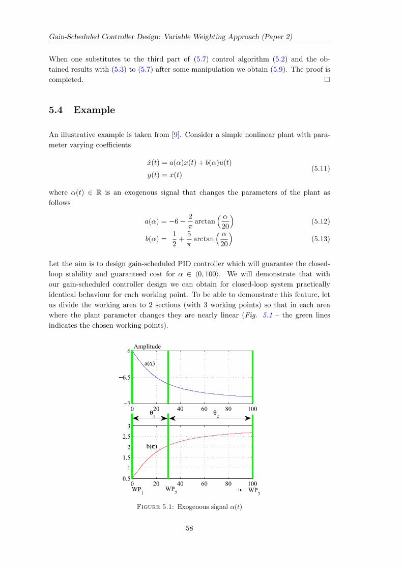
Gain-Scheduled Controller Design: Variable Weighting Approach (Paper 2)
When one substitutes to the third part of (5.7) control algorithm (5.2) and the ob-
tained results with (5.3) to (5.7) after some manipulation we obtain (5.9). The proof is
completed.
5.4 Example
An illustrative example is taken from [9]. Consider a simple nonlinear plant with para-
meter varying coefficients
x(t) = a(α)x(t) + b(α)u(t)
y(t) = x(t)(5.11)
where α(t) ∈ R is an exogenous signal that changes the parameters of the plant as
follows
a(α) = −6− 2
πarctan
( α20
)(5.12)
b(α) =1
2+
5
πarctan
( α20
)(5.13)
Let the aim is to design gain-scheduled PID controller which will guarantee the closed-
loop stability and guaranteed cost for α ∈ 〈0, 100〉. We will demonstrate that with
our gain-scheduled controller design we can obtain for closed-loop system practically
identical behaviour for each working point. To be able to demonstrate this feature, let
us divide the working area to 2 sections (with 3 working points) so that in each area
where the plant parameter changes they are nearly linear (Fig. 5.1 – the green lines
indicates the chosen working points).
0 20 40 60 80 1007
6.5
6
0 20 40 60 80 1000.5
1
1.5
2
2.5
3
θ2
θ1
WP1
WP2 WP
3
Amplitude
a( )
b( )
Figure 5.1: Exogenous signal α(t)
58
5.4. Example
In these working points calculated transfer functions are:
Gs1|α=0 =0.5
s+ 6, Gs2|α=30 =
2.064
s+ 6.626
Gs3|α=100 =2.686
s+ 6.874,
(5.14)
Above transfer functions we transform to time domain to obtain scheduling model in the
form (5.1). The obtained model we extended for gain scheduled PID controller design.
The extended model is given as follows
A0 =
[−6.4370 0
1 0
], A1 =
[−0.3130 0
0 0
]
A2 =
[−0.1240 0
0 0
]
B0 =
[1.5930
0
], B1 =
[0.7820
0
]
B2 =
[0.3110
0
],
C =
[1 0
0 1
], D = 0
Using Theorem 5.1 with weighting matrices Qi = qiI, q1 = q2 = q3 = 1× 10⁻⁴, R = rI,
r = 1, Si = siI, s1 = s2 = s3 = 1× 10⁻⁷ we obtain gain scheduled controller in the form
GrGS = Gr0 +Gr1θ1 +Gr2θ2 (5.15)
where
Gr0 =0.3033s2 + 2.3036s+ 2.0949
s
Gr1 = −3.93× 10⁻⁶s2 + 8.86× 10⁻⁵s+ 3.13× 10⁻⁵
s
Gr2 = −0.0724s2 + 1.6323s+ 0.5773
s
Simulation results (Figs. 5.2, 5.3) confirm, that Theorem 5.1 holds, but we can see also
that with equal qi, si we don’t obtain identical behaviour in each working point.
We can change the weighting matrices in the 1. working point to get required per-
formance quality. An another gain-scheduled controller was obtained with weighting
matrices Qi = qiI, q1 = 1 × 10⁻², q2 = q3 = 1 × 10⁻⁴ R = rI, r = 1, Si = siI,
s1 = s2 = s3 = 1× 10⁻⁷
GrGS = Gr0 +Gr1θ1 +Gr2θ2 (5.16)
59
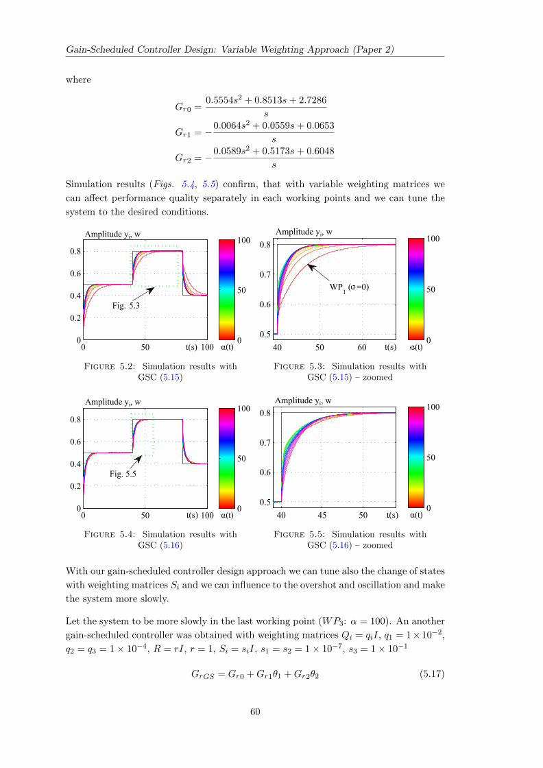
Gain-Scheduled Controller Design: Variable Weighting Approach (Paper 2)
where
Gr0 =0.5554s2 + 0.8513s+ 2.7286
s
Gr1 = −0.0064s2 + 0.0559s+ 0.0653
s
Gr2 = −0.0589s2 + 0.5173s+ 0.6048
s
Simulation results (Figs. 5.4, 5.5) confirm, that with variable weighting matrices we
can affect performance quality separately in each working points and we can tune the
system to the desired conditions.
0 50 1000
0.2
0.4
0.6
0.8
(t)0
50
100
Fig.
Amplitude yi, w
t(s)
5.3
α
Figure 5.2: Simulation results withGSC (5.15)
40 50 60
0.5
0.6
0.7
0.8
(t)0
50
100
WP1
( =0)
Amplitude yi, w
t(s)
Figure 5.3: Simulation results withGSC (5.15) – zoomed
0 50 1000
0.2
0.4
0.6
0.8
(t)0
50
100
Fig. 5.5
Amplitude yi, w
t(s) α
Figure 5.4: Simulation results withGSC (5.16)
40 45 50
0.5
0.6
0.7
0.8
(t)0
50
100Amplitude yi, w
t(s) α
Figure 5.5: Simulation results withGSC (5.16) – zoomed
With our gain-scheduled controller design approach we can tune also the change of states
with weighting matrices Si and we can influence to the overshot and oscillation and make
the system more slowly.
Let the system to be more slowly in the last working point (WP3: α = 100). An another
gain-scheduled controller was obtained with weighting matrices Qi = qiI, q1 = 1×10⁻²,
q2 = q3 = 1× 10⁻⁴, R = rI, r = 1, Si = siI, s1 = s2 = 1× 10⁻⁷, s3 = 1× 10⁻¹
GrGS = Gr0 +Gr1θ1 +Gr2θ2 (5.17)
60
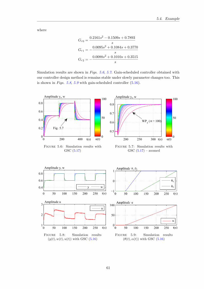
5.4. Example
where
Gr0 =0.2161s2 − 0.1509s+ 0.7893
s
Gr1 = −0.0095s2 + 0.1084s+ 0.3770
s
Gr2 = −0.0088s2 + 0.1010s+ 0.3515
s
Simulation results are shown in Figs. 5.6, 5.7. Gain-scheduled controller obtained with
our controller design method is remains stable under slowly parameter changes too. This
is shown in Figs. 5.8, 5.9 with gain-scheduled controller (5.16).
0 200 4000
0.2
0.4
0.6
0.8
(t)0
50
100
Fig.
Amplitude yi, w
t(s)
5.7
α
Figure 5.6: Simulation results withGSC (5.17)
200 250 300
0.5
0.6
0.7
0.8
(t)0
50
100
WP3
( = 100)
t(s)
Amplitude yi, w
α
α
Figure 5.7: Simulation results withGSC (5.17) – zoomed
0 50 100 150 200 250
0.4
0.6
0.8
y w
0 50 100 150 200 2501
2
3
u
Amplitude y, w
Amplitude u
t(s)
t(s)
Figure 5.8: Simulation results(y(t), w(t), u(t)) with GSC (5.16)
Figure 5.9: Simulation results(θ(t), α(t)) with GSC (5.16)
61
Gain-Scheduled Controller Design: Variable Weighting Approach (Paper 2)
5.5 Conclusion
This paper addresses the problem to design gain-scheduled controller which guarantee
the closed-loop stability and performance for all scheduled parameter changes. The pro-
posed original procedure is based on Lyapunov theory of stability, notion of guaranteed
cost and BMI. Using original variable weighting matrices we can affect performance
quality separately in each working points and we can tune the system to the desired
condition through all parameter changes. Numerical example illustrate the effectiveness
of the proposed approach.
Bibliography
[1] M. Sato, Brief paper: Gain-scheduled output-feedback controllers depending solely
on scheduling parameters via parameter-dependent Lyapunov functions, Automatica
47 (12) (2011) 2786–2790.
[2] H. Koroglu, Robust generalized asymptotic regulation via an LPV controller without
parameter derivative dependence, in: 49th IEEE Conference on Decision and Control
(CDC), 2010, 2010, pp. 4965–4971.
[3] F. Wang, V. Balakrishnan, Improved stability analysis and gain-scheduled control-
ler synthesis for parameter-dependent systems, IEEE Transactions on Automatic
Control 47 (5) (2002) 720–734.
[4] D. J. Leith, W. E. Leithead, Survey of gain-scheduling analysis and design, Interna-
tional Journal of Control 73 (11) (2000) 1001–1025.
[5] W. J. Rugh, J. S. Shamma, A survey of research on gain-scheduling, Automatica 36
(2000) 1401–1425.
[6] P. Gahinet, P. Apkarian, M. Chilali, Affine parameter-dependent Lyapunov functions
and real parametric uncertainty, IEEE Transactions on Automatic Control 41 (3)
(1996) 436–442.
[7] J. Engwerda, A. Weeren, A result on output feedback linear quadratic control, Auto-
matica 44 (1) (2008) 265–271.
[8] P. Apkarian, P. Gahinet, G. Becker, Self-Scheduled H∞ Control of Linear Parameter-
Varying Systems: A Design Example, Automatica 31 (9) (1995) 1251–1261.
[9] G. E. Stewart, A Pragmatic Approach to Robust Gain Scheduling, in: 7th IFAC
Symposium on Robust Control Design, Vol. 7, Aalborg Congress & Culture Centre,
Denmark, 2012, pp. 355–362.
62
6
Design of Robust Gain-Scheduled
PI Controllers (Paper 3)
Abstract
A novel approach to robust gain-scheduled controller design is presented. The proposed
design procedure is based on the robust stability condition developed for an uncertain
LPV system model introduced in this paper. The feasible design procedures are ob-
tained in the form of BMI or LMI. The obtained design results and their properties are
illustrated on simulation examples.
Keywords: Gain-scheduled controller, robust controller, parameter-dependent Lya-
punov function, quadratic gain-scheduled cost function, LPV systems.
6.1 Introduction
Gain scheduling belongs to the most popular approaches to linear parameter varying
systems (LPV) control design. However, in the absence of corresponding results, this
design provides no guarantees of robust stability, performance or even nominal stability
of the overall gain-scheduled control [1]. In many applications, a controller must accom-
modate a plant with changing dynamics, where the dynamics is strongly dependent on
the operating conditions. Developing a nonlinear plant model, the gain-scheduled con-
troller can be designed by the standard approach described in [2], [3] and [4] using linear
controller design techniques. In such cases, the designed gain-scheduled controller must
be able to stabilize and guarantee a reasonable performance for all operating conditions.
The question remains, what happens with a closed-loop system if the developed physical
nonlinear model is not precise enough? In such a case, frequent in applications, there is
a need for robust controller to cope with model uncertainty. Various robust controller
design methods for gain-scheduled plant are available in literature. In [5] the authors
63
Design of Robust Gain-Scheduled PI Controllers (Paper 3)
consider the case where uncertainties of LPV system are modeled by diagonal matrix
with norm bounded unknown parameters. The control objectives are internal stability
and disturbance attenuation in the case of a bounded induced L2 norm. The authors in
[6], address the gain scheduling of separately designed controllers to form a robust linear
parameter varying controller for an LPV plant. That is, the intent is to integrate a set of
separately designed local controllers into a gain-scheduled controller with maximal quad-
ratic H∞ performance using the LMI approach. A robust PID controller is designed in
[7] for the condensing boiler problem. The main feature of the proposed method is that
the stability, robustness margins and some performance specifications are guaranteed by
linear constraints in the Nyquist diagram. The condensing boiler is described by first
order models with time delay. A design of gain-scheduled PI controller is presented in
[1] considering that the system uncertainty is assumed to be the difference between the
nonlinear model (assuming to be an exact model) and the nominal linear model. Addi-
tionally, the input constraints problem is explicitly addressed in this paper.In the article
[8] presents the central finite-dimensional H∞ controller for linear time-varying systems
with unknown parameters, that is suboptimal for a given threshold with respect to a
modified Bolza-Meyer quadratic criterion including the attenuation control term with
the opposite sign. The paper [9] is concerned with the problem of the robust H∞ filter-
ing design for singular linear parameter varying systems with time variant delays. The
obtained results are proposed in terms of linear matrix inequality. In [10], the problem
of attenuation of sinusoidal disturbances with uncertain and arbitrarily time-varying fre-
quencies is solved by synthesis of LPV controllers using the L2 - gain method. A robust
gain-scheduled design procedure based on L2 controller synthesis method is proposed for
LPV systems in [11].The gap matrix approach to the design of a robust gain-scheduled
controller for LPV systems is studied in [12]. In [13], quadratic and bi-quadratic (affine)
stability approaches are used to design the gain-scheduled controller for each vertex of
the plant uncertainty box and the stability of the closed-loop system is verified by LMI.
In [14], a commercially available and vertically designed rotor bearing system is modeled
and controlled using an LMI and H∞ based gain-scheduled controller. The paper[15]
addresses the problem to gain scheduled controller design when scheduling parameters
are belong to the bounded uncertainties. The contribution of [16] is to use standard
results motivated by Youla-Kucera parametrization to propose a controller structure
and design approach that allows the gain scheduling of linear system such that a ro-
bustly stable nonlinear control system is achieved. In [17] provides a novel approach to
design continuous time varying H∞ gain-scheduled worst-case controllers for nonlinear
stochastic systems subject to partially known transition jump rates and actuator sat-
uration. The above short survey motivated us to study the following research problem
which has not been sufficiently solved yet. Design the robust gain-scheduled controller
which will guarantee:
• stability and robustness properties of the closed-loop system when the uncertain
plant parameters Π for all scheduled parameters θ ∈ Ωs and their rate θ ∈ Ωt lie in
the given polytopic (convex) uncertainty box Ω, that is Π ∈ Ω, θ ∈ Ωs and θ ∈ Ωt;
64
6.2. Problem formulation and preliminaries
• performance (guaranteed cost) for closed-loop system for all Π ∈ Ω, θ ∈ Ωs and
θ ∈ Ωt;
• parameter dependent quadratic stability.
In this paper, we provide, to the authors’ best knowledge, an alternative novel approach
to the robust gain-scheduled control problem. The proposed LPV uncertainty model,
introduced in Section 6.2, is used to formulate a robust gain scheduling control problem.
The main result is presented in Section 6.3. The design procedure is based on the new
developed robust stability condition for the gain-scheduled controller. In Section 6.4 the
LMI gain-scheduled controller design is presented and in Section 6.5, numerical examples
illustrate the effectiveness of the proposed approaches.
6.2 Problem formulation and preliminaries
Consider a linear continuous time parameter varying (LPV) uncertain system
x = A (ξ, θ)x+ B (ξ, θ)u
y = Cx(6.1)
where parameter varying system matrices are affine with respect to scheduled para-
meter θ
A (ξ, θ) = A0 (ξ) +s∑i=1
Ai (ξ) θi ∈ Rn×n
B (ξ, θ) = B0 (ξ) +s∑i=1
Bi (ξ) θi ∈ Rn×m(6.2)
x ∈ Rn, u ∈ Rm, y ∈ Rl denote the state, control input and controlled output, respect-
ively. Matrices Ai (ξ), Bi (ξ), i = 0, 1, . . . s belong to the convex and bounded set: a
polytope with N vertices that can be formally defined as
Ω :=Ai(ξ) ∈ Rn×n, Bi(ξ) ∈ Rn×m : Ai(ξ), Bi(ξ) :=
N∑j=1
(Aij , Bij) ξj ,N∑j=1
ξj = 1, ξj ≥ 0(6.3)
where s is the number of scheduled parameters; ξj , j = 1, 2, . . . , N are constant but un-
known parameters respective to uncertainties in system matrices Ai(ξ), Bi(ξ); Aij , Bij ,
C are constant matrices of corresponding dimensions respective to uncertainty polytope
vertices; θ ∈ Rs is a vector of known constant or possible time-varying real gain schedul-
ing parameters. We assume that both lower and upper bounds are available for these
parameters’ value and variation rates. Specifically
65
Design of Robust Gain-Scheduled PI Controllers (Paper 3)
• Each parameter θi, i = 1, 2, . . . , s ranges between known extremal values
θi ∈ Ωs :=θi ∈
⟨θi, θi
⟩, i = 1, 2, · · · s
. (6.4)
• The rate of variation θi is well defined at all times and satisfies
θi ∈ Ωt :=θi ∈
⟨θi, θi
⟩, i = 1, 2, . . . s
. (6.5)
Note that system (6.1) consists of two type vertices. The first one is due to the gain-
scheduled parameter θ with T = 2s vertices, θ – vertices and second set of vertices
are due to the system uncertainties, N vertices – ξ vertices. For the gain-scheduled I
part controller design the states of system (6.1) need to be extended in such a way that
the static output feedback control algorithm can provide proportional (P ) and integral
(I) parts of the designed PI robust controller. For more detail see [18]. Assume that
system (6.1) allows to design the PI controller with static output feedback. The following
problem is studied in this paper for the class of uncertain LPV systems (6.1).
Problem 6.1. Design a robust output feedback gain-scheduled PI controller with control
algorithm
u =
(F0 +
s∑i=1
Fiθi
)y = F (θ)Cx (6.6)
such that the controller guarantees robust parameter dependent quadratic stability and
guaranteed cost with respect to the performance index (6.8) for the respective closed-
loop system (6.7) with convex uncertainty domain (6.3)
x =(A(ξ, θ) + B(ξ, θ)F (θ)C
)x = Ac(ξ, θ)x (6.7)
To assess the performance quality, a quadratic cost function known from LQ theory is
used
Jc =
∫ ∞0
(xTQx+ uTRu
)dt =
∫ ∞0
J(t)dt (6.8)
The respective notion of guaranteed cost is given in the next definition.
Definition 6.1. Consider system (6.1) and controller (6.6). If there exist a control law
u∗ and a positive scalar J∗ such that the respective closed-loop system (6.7) is stable
and the value of the closed-loop cost function (6.8) satisfies Jc ≤ J∗, then J∗ is said to
be guaranteed cost and u∗ is said to be the guaranteed cost control law for system (6.1).
Recall the well known result from LQ theory which will be used below to prove one of
the main results.
Lemma 6.1. [19] Consider the system (6.1) with control algorithm (6.6). Control al-
gorithm (6.6) is the guaranteed cost control law for the closed-loop system (6.7) if and
66
6.3. Main results
only if there exists a parameter dependent Lyapunov function V (ξ, θ) such that the fol-
lowing condition holds
Be(ξ, θ) = minu
(dV (ξ, θ, u)
dt+ J(t)
)≤ 0 (6.9)
Uncertain system (6.1) with control algorithm (6.6) conforming to Lemma 6.1 is called
robust parameter dependent quadratically stable with guaranteed cost.
We proceed with the notion of multi-convexity of a scalar quadratic function, and its
qualities classified in the next lemma, [20].
Lemma 6.2. Consider a scalar quadratic function of θ ∈ Rs
f(θ) = α0 +s∑i=1
αiθi +s∑i=1
s∑j>i
βijθiθj +s∑i=1
γiθ2i (6.10)
and assume that f(·) is multiconvex, that is ∂2f∂θ2i
= 2γi ≥ 0, i = 1, 2, · · · s. Then f(·) is
negative in the hyper rectangle (6.4) if and only if it takes negative values at the corners
of (6.4), that is, if and only if f(θ) < 0 for all vertices of the set given by (6.4).
6.3 Main results
This section formulates the theoretical approach to the robust gain-scheduled controller
design for polytopic system (6.1) which ensures closed-loop system parameter dependent
quadratic stability and guaranteed cost (6.8), for all uncertain plant parameters Π ∈ Ω,
gain scheduling parameters θ ∈ Ωs and θ ∈ Ωt. The main result on robust stability for
the gain-scheduled control system is given in the next theorem.
Theorem 6.1. The closed-loop system (6.7) is robust parameter dependent quadratically
stabilizable with guaranteed cost if there exist a positive definite matrix P (ξ, θ) ∈ Rn×n,
matrices N1, N2 ∈ Rn×n and gain-scheduled controller (6.6) such that
a)
L(ξ, θ) = M0(ξ) +s∑i=1
Mi(ξ)θi
+s∑i=1
s∑j>i
Mij(ξ)θiθj +s∑i=1
Mii(ξ)θ2i < 0
(6.11)
b)
Mii(ξ) ≥ 0, (6.12)
i = 1, 2, . . . , s ∀θ ∈ Ωs, θ ∈ Ωt,
N∑j=1
ξj = 1, ξj ≥ 0
67
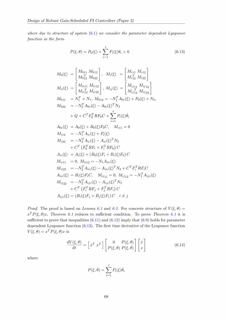
Design of Robust Gain-Scheduled PI Controllers (Paper 3)
where due to structure of system (6.1) we consider the parameter dependent Lyapunov
function in the form
P (ξ, θ) = P0(ξ) +
s∑i=1
Pi(ξ)θi > 0 (6.13)
M0(ξ) =
[M011 M012
M0T12 M022
], Mi(ξ) =
[Mi11 Mi12
MiT12 Mi22
]
Mii(ξ) =
[Mii11 Mii12
MiiT12 Mii22
], Mij(ξ) =
[Mij11 Mij12
MijT12 Mij22
]M011 = NT
1 +N1, M012 = −NT1 A0c(ξ) + P0(ξ) +N2,
M022 = −NT2 A0c(ξ)−A0c(ξ)
TN2
+Q+ CTF T0 RF0C +s∑i=1
Pi(ξ)θi
A0c(ξ) = A0(ξ) +B0(ξ)F0C, Mi11 = 0
Mi12 = −NT1 Aic(ξ) + Pi(ξ)
Mi22 = −NT2 Aic(ξ)−Aic(ξ)TN2
+ CT(F T0 RFi + F Ti RF0
)C
Aic(ξ) = Ai(ξ) + (B0(ξ)Fi +Bi(ξ)F0)C
Mii11 = 0, Mii12 = −N1Aiic(ξ)
Mii22 = −NT2 Aiic(ξ)−Aiic(ξ)TN2 + CTF Ti RFiC
Aiic(ξ) = Bi(ξ)FiC, Mij11 = 0, Mij12 = −NT1 Aijc(ξ)
Mij22 = −NT2 Aijc(ξ)−Aijc(ξ)TN2
+ CT(F Ti RFj + F Tj RFi
)C
Aijc(ξ) = (Bi(ξ)Fj +Bj(ξ)Fi)C i 6= j
Proof. The proof is based on Lemma 6.1 and 6.2. For concrete structure of V (ξ, θ) =
xTP (ξ, θ)x, Theorem 6.1 reduces to sufficient condition. To prove Theorem 6.1 it is
sufficient to prove that inequalities (6.11) and (6.12) imply that (6.9) holds for parameter
dependent Lyapunov function (6.13). The first time derivative of the Lyapunov function
V (ξ, θ) = xTP (ξ, θ)x is
dV (ξ, θ)
dt=[xT xT
] [ 0 P (ξ, θ)
P (ξ, θ) P (ξ, θ)
][x
x
](6.14)
where
P (ξ, θ) =s∑i=1
Pi(ξ)θi
68
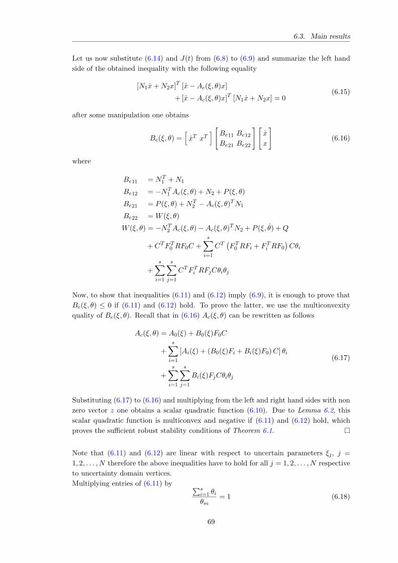
6.3. Main results
Let us now substitute (6.14) and J(t) from (6.8) to (6.9) and summarize the left hand
side of the obtained inequality with the following equality
[N1x+N2x]T [x−Ac(ξ, θ)x]
+ [x−Ac(ξ, θ)x]T [N1x+N2x] = 0(6.15)
after some manipulation one obtains
Be(ξ, θ) =[xT xT
] [Be11 Be12
Be21 Be22
][x
x
](6.16)
where
Be11 = NT1 +N1
Be12 = −NT1 Ac(ξ, θ) +N2 + P (ξ, θ)
Be21 = P (ξ, θ) +NT2 −Ac(ξ, θ)TN1
Be22 = W (ξ, θ)
W (ξ, θ) = −NT2 Ac(ξ, θ)−Ac(ξ, θ)TN2 + P (ξ, θ) +Q
+ CTF T0 RF0C +s∑i=1
CT(F T0 RFi + F Ti RF0
)Cθi
+s∑i=1
s∑j=1
CTF Ti RFjCθiθj
Now, to show that inequalities (6.11) and (6.12) imply (6.9), it is enough to prove that
Be(ξ, θ) ≤ 0 if (6.11) and (6.12) hold. To prove the latter, we use the multiconvexity
quality of Be(ξ, θ). Recall that in (6.16) Ac(ξ, θ) can be rewritten as follows
Ac(ξ, θ) = A0(ξ) +B0(ξ)F0C
+
s∑i=1
[Ai(ξ) + (B0(ξ)Fi +Bi(ξ)F0)C] θi
+
s∑i=1
s∑j=1
Bi(ξ)FjCθiθj
(6.17)
Substituting (6.17) to (6.16) and multiplying from the left and right hand sides with non
zero vector z one obtains a scalar quadratic function (6.10). Due to Lemma 6.2, this
scalar quadratic function is multiconvex and negative if (6.11) and (6.12) hold, which
proves the sufficient robust stability conditions of Theorem 6.1.
Note that (6.11) and (6.12) are linear with respect to uncertain parameters ξj , j =
1, 2, . . . , N therefore the above inequalities have to hold for all j = 1, 2, . . . , N respective
to uncertainty domain vertices.
Multiplying entries of (6.11) by ∑si=1 θiθm
= 1 (6.18)
69
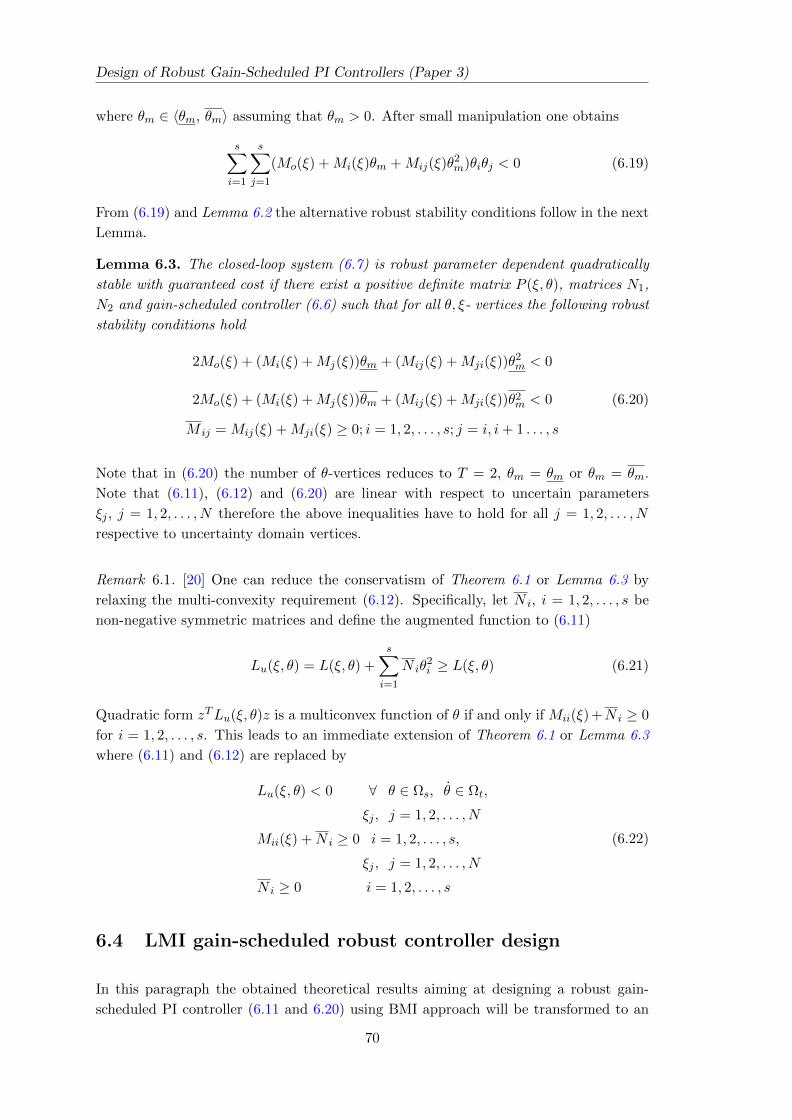
Design of Robust Gain-Scheduled PI Controllers (Paper 3)
where θm ∈ 〈θm, θm〉 assuming that θm > 0. After small manipulation one obtains
s∑i=1
s∑j=1
(Mo(ξ) +Mi(ξ)θm +Mij(ξ)θ2m)θiθj < 0 (6.19)
From (6.19) and Lemma 6.2 the alternative robust stability conditions follow in the next
Lemma.
Lemma 6.3. The closed-loop system (6.7) is robust parameter dependent quadratically
stable with guaranteed cost if there exist a positive definite matrix P (ξ, θ), matrices N1,
N2 and gain-scheduled controller (6.6) such that for all θ, ξ- vertices the following robust
stability conditions hold
2Mo(ξ) + (Mi(ξ) +Mj(ξ))θm + (Mij(ξ) +Mji(ξ))θ2m < 0
2Mo(ξ) + (Mi(ξ) +Mj(ξ))θm + (Mij(ξ) +Mji(ξ))θ2m < 0 (6.20)
M ij = Mij(ξ) +Mji(ξ) ≥ 0; i = 1, 2, . . . , s; j = i, i+ 1 . . . , s
Note that in (6.20) the number of θ-vertices reduces to T = 2, θm = θm or θm = θm.
Note that (6.11), (6.12) and (6.20) are linear with respect to uncertain parameters
ξj , j = 1, 2, . . . , N therefore the above inequalities have to hold for all j = 1, 2, . . . , N
respective to uncertainty domain vertices.
Remark 6.1. [20] One can reduce the conservatism of Theorem 6.1 or Lemma 6.3 by
relaxing the multi-convexity requirement (6.12). Specifically, let N i, i = 1, 2, . . . , s be
non-negative symmetric matrices and define the augmented function to (6.11)
Lu(ξ, θ) = L(ξ, θ) +
s∑i=1
N iθ2i ≥ L(ξ, θ) (6.21)
Quadratic form zTLu(ξ, θ)z is a multiconvex function of θ if and only if Mii(ξ) +N i ≥ 0
for i = 1, 2, . . . , s. This leads to an immediate extension of Theorem 6.1 or Lemma 6.3
where (6.11) and (6.12) are replaced by
Lu(ξ, θ) < 0 ∀ θ ∈ Ωs, θ ∈ Ωt,
ξj , j = 1, 2, . . . , N
Mii(ξ) +N i ≥ 0 i = 1, 2, . . . , s,
ξj , j = 1, 2, . . . , N
N i ≥ 0 i = 1, 2, . . . , s
(6.22)
6.4 LMI gain-scheduled robust controller design
In this paragraph the obtained theoretical results aiming at designing a robust gain-
scheduled PI controller (6.11 and 6.20) using BMI approach will be transformed to an
70
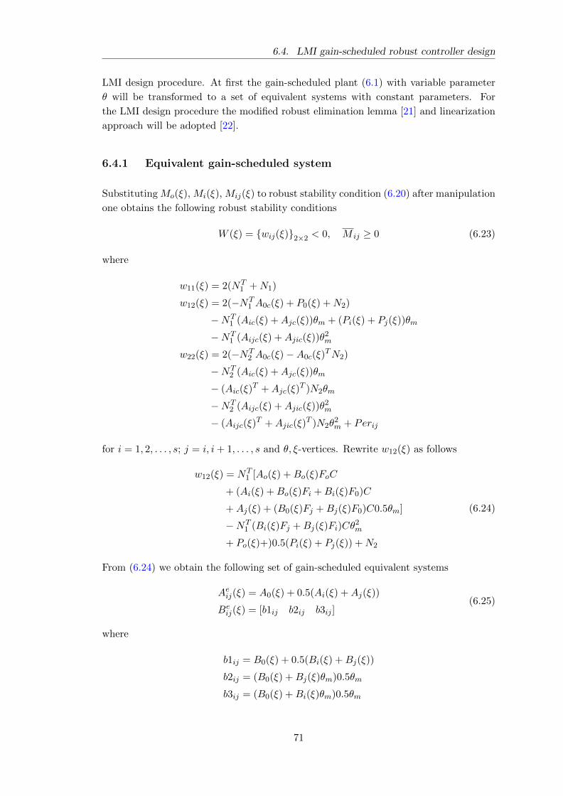
6.4. LMI gain-scheduled robust controller design
LMI design procedure. At first the gain-scheduled plant (6.1) with variable parameter
θ will be transformed to a set of equivalent systems with constant parameters. For
the LMI design procedure the modified robust elimination lemma [21] and linearization
approach will be adopted [22].
6.4.1 Equivalent gain-scheduled system
Substituting Mo(ξ), Mi(ξ), Mij(ξ) to robust stability condition (6.20) after manipulation
one obtains the following robust stability conditions
W (ξ) = wij(ξ)2×2 < 0, M ij ≥ 0 (6.23)
where
w11(ξ) = 2(NT1 +N1)
w12(ξ) = 2(−NT1 A0c(ξ) + P0(ξ) +N2)
−NT1 (Aic(ξ) +Ajc(ξ))θm + (Pi(ξ) + Pj(ξ))θm
−NT1 (Aijc(ξ) +Ajic(ξ))θ
2m
w22(ξ) = 2(−NT2 A0c(ξ)−A0c(ξ)
TN2)
−NT2 (Aic(ξ) +Ajc(ξ))θm
− (Aic(ξ)T +Ajc(ξ)
T )N2θm
−NT2 (Aijc(ξ) +Ajic(ξ))θ
2m
− (Aijc(ξ)T +Ajic(ξ)
T )N2θ2m + Perij
for i = 1, 2, . . . , s; j = i, i+ 1, . . . , s and θ, ξ-vertices. Rewrite w12(ξ) as follows
w12(ξ) = NT1 [Ao(ξ) +Bo(ξ)FoC
+ (Ai(ξ) +Bo(ξ)Fi +Bi(ξ)F0)C
+Aj(ξ) + (B0(ξ)Fj +Bj(ξ)F0)C0.5θm]
−NT1 (Bi(ξ)Fj +Bj(ξ)Fi)Cθ
2m
+ Po(ξ)+)0.5(Pi(ξ) + Pj(ξ)) +N2
(6.24)
From (6.24) we obtain the following set of gain-scheduled equivalent systems
Aeij(ξ) = A0(ξ) + 0.5(Ai(ξ) +Aj(ξ))
Beij(ξ) = [b1ij b2ij b3ij ]
(6.25)
where
b1ij = B0(ξ) + 0.5(Bi(ξ) +Bj(ξ))
b2ij = (B0(ξ) +Bj(ξ)θm)0.5θm
b3ij = (B0(ξ) +Bi(ξ)θm)0.5θm
71
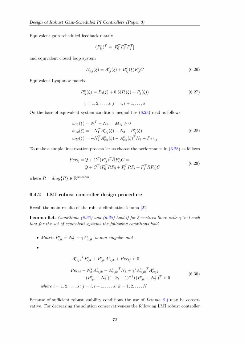
Design of Robust Gain-Scheduled PI Controllers (Paper 3)
Equivalent gain-scheduled feedback matrix
(F eij)T = [F T0 F
Ti F
Tj ]
and equivalent closed loop system
Aecij(ξ) = Aeij(ξ) +Beij(ξ)F
eijC (6.26)
Equivalent Lyapunov matrix
P eij(ξ) = P0(ξ) + 0.5(Pi(ξ) + Pj(ξ)) (6.27)
i = 1, 2, . . . , s; j = i, i+ 1, . . . , s
On the base of equivalent system condition inequalities (6.23) read as follows
w11(ξ) = NT1 +N1; M ij ≥ 0
w12(ξ) = −NT1 A
ecij(ξ) +N2 + P eij(ξ)
w22(ξ) = −NT2 A
ecij(ξ)−Aecij(ξ)TN2 + Perij
(6.28)
To make a simple linearization process let us choose the performance in (6.28) as follows
Perij =Q+ CT (F eij)T RF eijC =
Q+ CT (F T0 RF0 + F Ti RFi + F Tj RFj)C(6.29)
where R = diagR ∈ R3m×3m.
6.4.2 LMI robust controller design procedure
Recall the main results of the robust elimination lemma [21]
Lemma 6.4. Conditions (6.23) and (6.28) hold if for ξ-vertices there exits γ > 0 such
that for the set of equivalent systems the following conditions hold
• Matrix P eijk +NT2 − γAecijk is non singular and
•
AecijkTP eijk + P eijkA
ecijk + Perij < 0
Perij −NT2 A
ecijk −AecijkTN2 + γ2Aecijk
TAecijk
− (P eijk +NT2 )(−2γ + 1)−1I(P eijk +NT
2 )T < 0(6.30)
where i = 1, 2, . . . , s; j = i, i+ 1, . . . , s; k = 1, 2, . . . , N
Because of sufficient robust stability conditions the use of Lemma 6.4 may be conser-
vative. For decreasing the solution conservativeness the following LMI robust controller
72
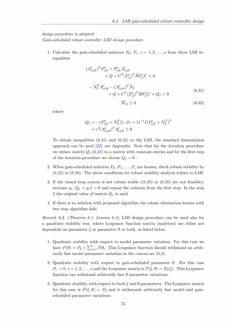
6.4. LMI gain-scheduled robust controller design
design procedure is adopted
Gain-scheduled robust controller LMI design procedure.
1. Calculate the gain-scheduled matrices F0, Fi, i = 1, 2, . . . , s from three LMI in-
equalities
(Aecijk)TP eijk + P eijkA
ecijk
+Q+ CT (F eij)T RF eijC < 0
−NT2 A
ecijk − (Aecijk)
TN2
+Q+ CT (F eij)T RF eijC +Q1 < 0
(6.31)
M ij ≥ 0 (6.32)
where
Q1 = −(P eijk +NT2 )(−2γ + 1)−1I(P eijk +NT
2 )T
+ γ2(Aecijk)TAecijk ≥ 0
To obtain inequalities (6.31) and (6.32) to the LMI, the standard linearization
approach can be used [22], see Appendix. Note that for the iteration procedure
we reduce matrix Q1 (6.31) to a matrix with constant entries and for the first step
of the iteration procedure we choose Q1 = 0 .
2. When gain-scheduled matrices F0, F1, . . . , Fs are known, check robust stability by
(6.23) or (6.28). The above conditions for robust stability analysis reduce to LMI.
3. If the closed loop system is not robust stable ((6.23) or (6.28) are not feasible),
increase q1, Q1 = q1I > 0 and repeat the solution from the first step. In the step
2 the original value of matrix Q1 is used.
4. If there is no solution with proposed algorithm the robust elimination lemma with
two step algorithm fails.
Remark 6.2. (Theorem 6.1, Lemma 6.3), LMI design procedure can be used also for
a quadratic stability test, where Lyapunov function matrix (matrices) are either not
dependent on parameter ξ or parameter θ or both, as listed below.
1. Quadratic stability with respect to model parameter variation. For this case we
have P (θ) = P0 +∑s
i=1 Piθi. This Lyapunov function should withstand an arbit-
rarily fast model parameter variation in the convex set (6.3).
2. Quadratic stability with respect to gain-scheduled parameter θ. For this case
Pi → 0, i = 1, 2, . . . , s and the Lyapunov matrix is P (ξ, θ) = P0(ξ). This Lyapunov
function can withstand arbitrarily fast θ parameter variations.
3. Quadratic stability with respect to both ξ and θ parameters. The Lyapunov matrix
for this case is P (ξ, θ) = P0 and it withstands arbitrarily fast model and gain-
scheduled parameter variations.
73
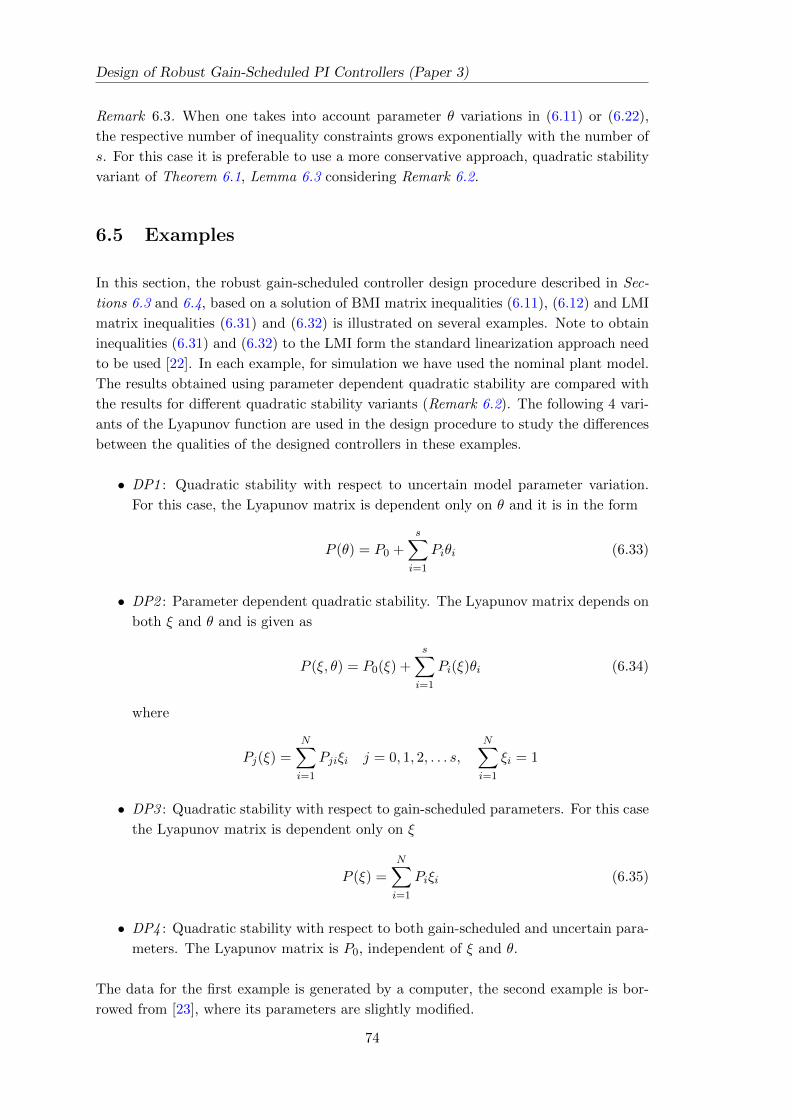
Design of Robust Gain-Scheduled PI Controllers (Paper 3)
Remark 6.3. When one takes into account parameter θ variations in (6.11) or (6.22),
the respective number of inequality constraints grows exponentially with the number of
s. For this case it is preferable to use a more conservative approach, quadratic stability
variant of Theorem 6.1, Lemma 6.3 considering Remark 6.2.
6.5 Examples
In this section, the robust gain-scheduled controller design procedure described in Sec-
tions 6.3 and 6.4, based on a solution of BMI matrix inequalities (6.11), (6.12) and LMI
matrix inequalities (6.31) and (6.32) is illustrated on several examples. Note to obtain
inequalities (6.31) and (6.32) to the LMI form the standard linearization approach need
to be used [22]. In each example, for simulation we have used the nominal plant model.
The results obtained using parameter dependent quadratic stability are compared with
the results for different quadratic stability variants (Remark 6.2). The following 4 vari-
ants of the Lyapunov function are used in the design procedure to study the differences
between the qualities of the designed controllers in these examples.
• DP1 : Quadratic stability with respect to uncertain model parameter variation.
For this case, the Lyapunov matrix is dependent only on θ and it is in the form
P (θ) = P0 +s∑i=1
Piθi (6.33)
• DP2 : Parameter dependent quadratic stability. The Lyapunov matrix depends on
both ξ and θ and is given as
P (ξ, θ) = P0(ξ) +s∑i=1
Pi(ξ)θi (6.34)
where
Pj(ξ) =
N∑i=1
Pjiξi j = 0, 1, 2, . . . s,
N∑i=1
ξi = 1
• DP3 : Quadratic stability with respect to gain-scheduled parameters. For this case
the Lyapunov matrix is dependent only on ξ
P (ξ) =
N∑i=1
Piξi (6.35)
• DP4 : Quadratic stability with respect to both gain-scheduled and uncertain para-
meters. The Lyapunov matrix is P0, independent of ξ and θ.
The data for the first example is generated by a computer, the second example is bor-
rowed from [23], where its parameters are slightly modified.
74
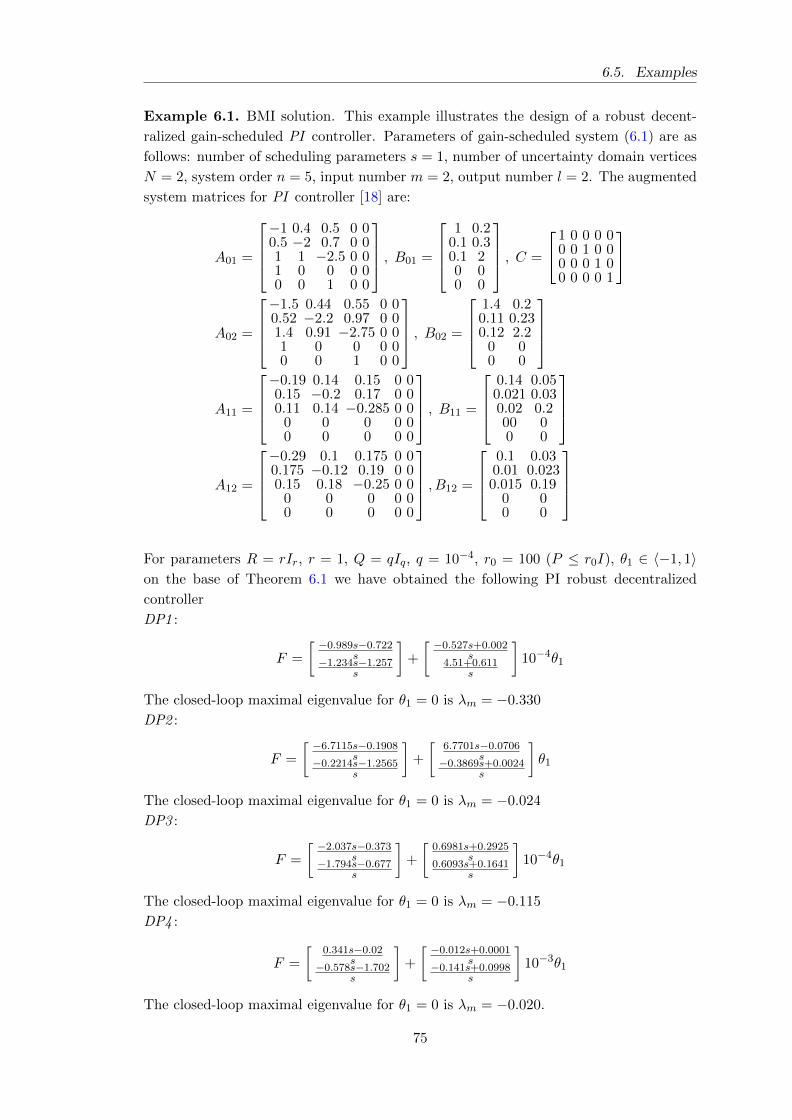
6.5. Examples
Example 6.1. BMI solution. This example illustrates the design of a robust decent-
ralized gain-scheduled PI controller. Parameters of gain-scheduled system (6.1) are as
follows: number of scheduling parameters s = 1, number of uncertainty domain vertices
N = 2, system order n = 5, input number m = 2, output number l = 2. The augmented
system matrices for PI controller [18] are:
A01 =
−1 0.4 0.5 0 00.5 −2 0.7 0 01 1 −2.5 0 01 0 0 0 00 0 1 0 0
, B01 =
1 0.2
0.1 0.30.1 20 00 0
, C =
1 0 0 0 00 0 1 0 00 0 0 1 00 0 0 0 1
A02 =
−1.5 0.44 0.55 0 00.52 −2.2 0.97 0 01.4 0.91 −2.75 0 01 0 0 0 00 0 1 0 0
, B02 =
1.4 0.20.11 0.230.12 2.2
0 00 0
A11 =
−0.19 0.14 0.15 0 00.15 −0.2 0.17 0 00.11 0.14 −0.285 0 0
0 0 0 0 00 0 0 0 0
, B11 =
0.14 0.050.021 0.030.02 0.200 00 0
A12 =
−0.29 0.1 0.175 0 00.175 −0.12 0.19 0 00.15 0.18 −0.25 0 0
0 0 0 0 00 0 0 0 0
, B12 =
0.1 0.030.01 0.0230.015 0.19
0 00 0
For parameters R = rIr, r = 1, Q = qIq, q = 10−4, r0 = 100 (P ≤ r0I), θ1 ∈ 〈−1, 1〉on the base of Theorem 6.1 we have obtained the following PI robust decentralized
controller
DP1 :
F =
[ −0.989s−0.722s−1.234s−1.257s
]+
[ −0.527s+0.002s
4.51+0.611s
]10−4θ1
The closed-loop maximal eigenvalue for θ1 = 0 is λm = −0.330
DP2 :
F =
[ −6.7115s−0.1908s−0.2214s−1.2565s
]+
[6.7701s−0.0706
s−0.3869s+0.0024s
]θ1
The closed-loop maximal eigenvalue for θ1 = 0 is λm = −0.024
DP3 :
F =
[ −2.037s−0.373s−1.794s−0.677s
]+
[0.6981s+0.2925
s0.6093s+0.1641
s
]10−4θ1
The closed-loop maximal eigenvalue for θ1 = 0 is λm = −0.115
DP4 :
F =
[0.341s−0.02
s−0.578s−1.702s
]+
[ −0.012s+0.0001s−0.141s+0.0998s
]10−3θ1
The closed-loop maximal eigenvalue for θ1 = 0 is λm = −0.020.
75
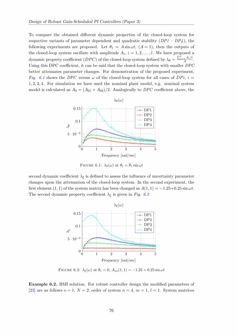
Design of Robust Gain-Scheduled PI Controllers (Paper 3)
To compare the obtained different dynamic properties of the closed-loop system for
respective variants of parameter dependent and quadratic stability (DP1 – DP4 ), the
following experiments are proposed. Let θ1 = A sinωt, (A = 1), then the outputs of
the closed-loop system oscillate with amplitude Ai, i = 1, 2, . . . , l. We have proposed a
dynamic property coefficient (DPC) of the closed-loop system defined by λθ =∑l
i=1 Ai/lA .
Using this DPC coefficient, it can be said that the closed-loop system with smaller DPC
better attenuates parameter changes. For demonstration of the proposed experiment,
Fig. 6.1 shows the DPC versus ω of the closed-loop system for all cases of DPi, i =
1, 2, 3, 4. For simulation we have used the nominal plant model, e.g. nominal system
model is calculated as A0 = (A01 + A02)/2. Analogically to DPC coefficient above, the
0 1 2 3 4 50
5 · 10−2
0.1
0.15
Frequency [rad/sec]
λθ
λθ(ω)
DP1DP2DP3DP4
Figure 6.1: λθ(ω) at θ1 = θ1 sinωt
second dynamic coefficient λξ is defined to assess the influence of uncertainty parameter
changes upon the attenuation of the closed-loop system. In the second experiment, the
first element (1, 1) of the system matrix has been changed as A(1, 1) = −1.25+0.25 sinωt.
The second dynamic property coefficient λξ is given in Fig. 6.2
0 1 2 3 4 50
5 · 10−2
0.1
0.15
Frequency [rad/sec]
λξ
λξ(ω)
DP1DP2DP3DP4
Figure 6.2: λξ(ω) at θ1 = 0, Ano(1, 1) = −1.25 + 0.25 sinωt
Example 6.2. BMI solution. For robust controller design the modified parameters of
[23] are as follows s = 1, N = 2, order of system n = 4, m = 1, l = 1. System matrices
76
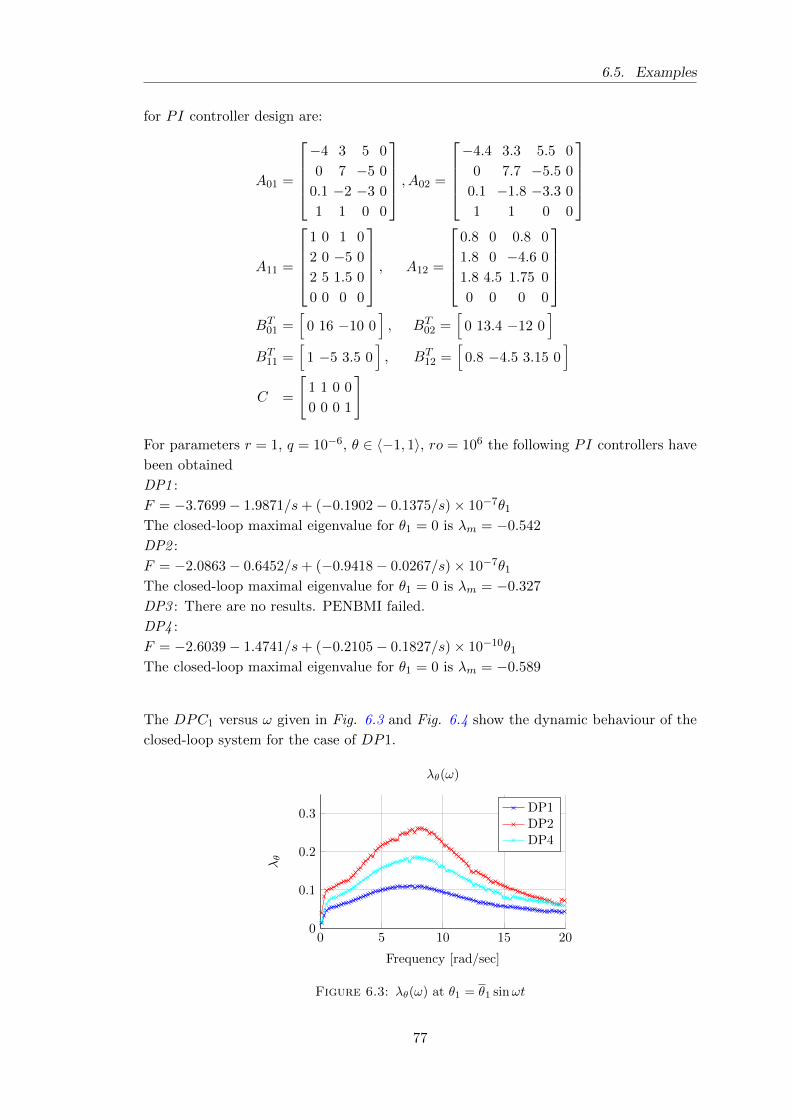
6.5. Examples
for PI controller design are:
A01 =
−4 3 5 0
0 7 −5 0
0.1 −2 −3 0
1 1 0 0
, A02 =
−4.4 3.3 5.5 0
0 7.7 −5.5 0
0.1 −1.8 −3.3 0
1 1 0 0
A11 =
1 0 1 0
2 0 −5 0
2 5 1.5 0
0 0 0 0
, A12 =
0.8 0 0.8 0
1.8 0 −4.6 0
1.8 4.5 1.75 0
0 0 0 0
BT
01 =[
0 16 −10 0], BT
02 =[
0 13.4 −12 0]
BT11 =
[1 −5 3.5 0
], BT
12 =[
0.8 −4.5 3.15 0]
C =
[1 1 0 0
0 0 0 1
]
For parameters r = 1, q = 10−6, θ ∈ 〈−1, 1〉, ro = 106 the following PI controllers have
been obtained
DP1 :
F = −3.7699− 1.9871/s+ (−0.1902− 0.1375/s)× 10−7θ1
The closed-loop maximal eigenvalue for θ1 = 0 is λm = −0.542
DP2 :
F = −2.0863− 0.6452/s+ (−0.9418− 0.0267/s)× 10−7θ1
The closed-loop maximal eigenvalue for θ1 = 0 is λm = −0.327
DP3 : There are no results. PENBMI failed.
DP4 :
F = −2.6039− 1.4741/s+ (−0.2105− 0.1827/s)× 10−10θ1
The closed-loop maximal eigenvalue for θ1 = 0 is λm = −0.589
The DPC1 versus ω given in Fig. 6.3 and Fig. 6.4 show the dynamic behaviour of the
closed-loop system for the case of DP1.
0 5 10 15 200
0.1
0.2
0.3
Frequency [rad/sec]
λθ
λθ(ω)
DP1DP2DP4
Figure 6.3: λθ(ω) at θ1 = θ1 sinωt
77
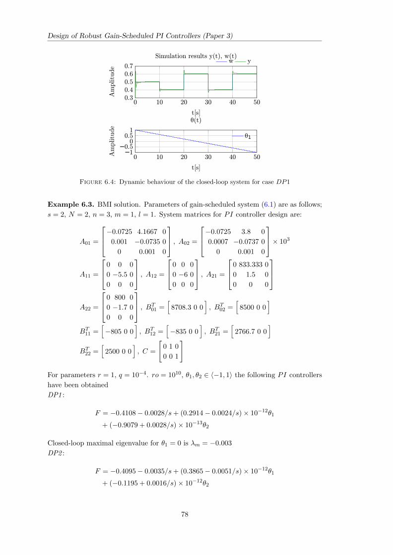
Design of Robust Gain-Scheduled PI Controllers (Paper 3)
0 10 20 30 40 500.30.40.50.60.7
t[s]Amplitude
Simulation results y(t), w(t)w y
0 10 20 30 40 50−1
−0.50
0.51
t[s]
Amplitude
θ(t)
θ1
Figure 6.4: Dynamic behaviour of the closed-loop system for case DP1
Example 6.3. BMI solution. Parameters of gain-scheduled system (6.1) are as follows;
s = 2, N = 2, n = 3, m = 1, l = 1. System matrices for PI controller design are:
A01 =
−0.0725 4.1667 0
0.001 −0.0735 0
0 0.001 0
, A02 =
−0.0725 3.8 0
0.0007 −0.0737 0
0 0.001 0
× 103
A11 =
0 0 0
0 −5.5 0
0 0 0
, A12 =
0 0 0
0 −6 0
0 0 0
, A21 =
0 833.333 0
0 1.5 0
0 0 0
A22 =
0 800 0
0 −1.7 0
0 0 0
, BT01 =
[8708.3 0 0
], BT
02 =[
8500 0 0]
BT11 =
[−805 0 0
], BT
12 =[−835 0 0
], BT
21 =[
2766.7 0 0]
BT22 =
[2500 0 0
], C =
[0 1 0
0 0 1
]
For parameters r = 1, q = 10−4. ro = 1010, θ1, θ2 ∈ 〈−1, 1〉 the following PI controllers
have been obtained
DP1 :
F = −0.4108− 0.0028/s+ (0.2914− 0.0024/s)× 10−12θ1
+ (−0.9079 + 0.0028/s)× 10−13θ2
Closed-loop maximal eigenvalue for θ1 = 0 is λm = −0.003
DP2 :
F = −0.4095− 0.0035/s+ (0.3865− 0.0051/s)× 10−12θ1
+ (−0.1195 + 0.0016/s)× 10−12θ2
78
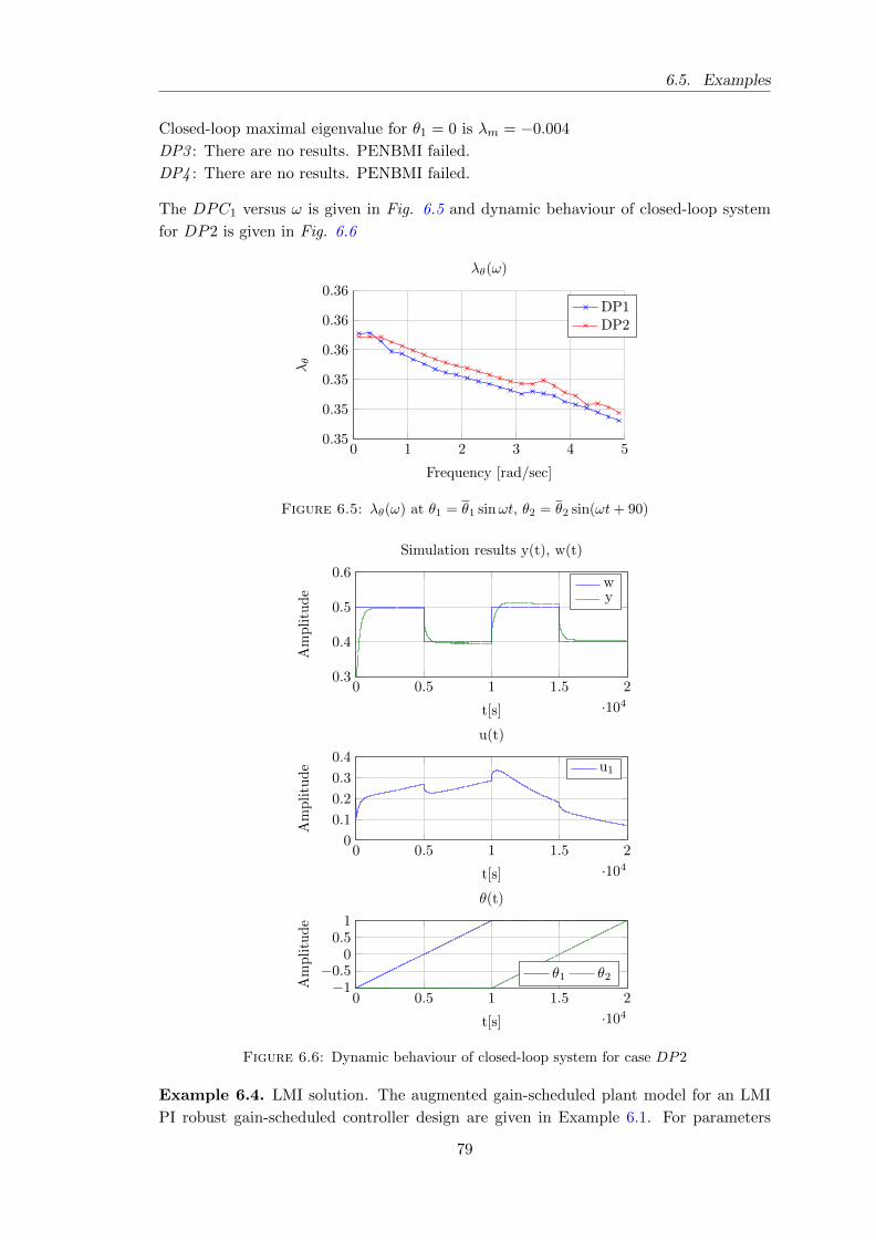
6.5. Examples
Closed-loop maximal eigenvalue for θ1 = 0 is λm = −0.004
DP3 : There are no results. PENBMI failed.
DP4 : There are no results. PENBMI failed.
The DPC1 versus ω is given in Fig. 6.5 and dynamic behaviour of closed-loop system
for DP2 is given in Fig. 6.6
0 1 2 3 4 50.35
0.35
0.35
0.36
0.36
0.36
Frequency [rad/sec]
λθ
λθ(ω)
DP1DP2
Figure 6.5: λθ(ω) at θ1 = θ1 sinωt, θ2 = θ2 sin(ωt+ 90)
0 0.5 1 1.5 2
·1040
0.1
0.2
0.3
0.4
t[s]
Amplitude
u(t)
u1
0 0.5 1 1.5 2
·1040.3
0.4
0.5
0.6
t[s]
Amplitude
Simulation results y(t), w(t)
wy
0 0.5 1 1.5 2
·104−1
−0.50
0.51
t[s]
Amplitude
θ(t)
θ1 θ2
Figure 6.6: Dynamic behaviour of closed-loop system for case DP2
Example 6.4. LMI solution. The augmented gain-scheduled plant model for an LMI
PI robust gain-scheduled controller design are given in Example 6.1. For parameters
79
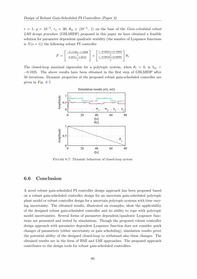
Design of Robust Gain-Scheduled PI Controllers (Paper 3)
r = 1, q = 10−5, ro = 30, θm ∈ 〈10−5, 1〉 on the base of the Gain-scheduled robust
LMI design procedure (GSLMIDP) proposed in this paper we have obtained a feasible
solution for parameter dependent quadratic stability (the number of Lyapunov functions
is N(s+ 1)) the following robust PI controller
F =
[−0.1148s−1.5886
s0.257s−1.0515
s
]+
[(−0.0921s+0.1068)
s(−0.0918s+0.0908)
s
]θ1
The closed-loop maximal eigenvalue for a polytopic system, when θ1 = 0, is λm =
−0.1825. The above results have been obtained in the first step of GSLMIDP after
50 iterations. Dynamic properties of the proposed robust gain-scheduled controller are
given in Fig. 6.7.
0 20 40 60 80
0
0.5
1
t[s]
Am
pli
tude
Simulation results y(t), w(t)
w2
y1
y2
0 20 40 60 800
0.5
1
t[s]
Am
pli
tude
θ(t)
θ1
w1
Figure 6.7: Dynamic behaviour of closed-loop system
6.6 Conclusion
A novel robust gain-scheduled PI controller design approach has been proposed based
on a robust gain-scheduled controller design for an uncertain gain-scheduled polytopic
plant model or robust controller design for a uncertain polytopic systems with time vary-
ing uncertainty. The obtained results, illustrated on examples, show the applicability
of the designed robust gain-scheduled controller and its ability to cope with polytopic
model uncertainties. Several forms of parameter dependent/quadratic Lyapunov func-
tions are presented and tested by simulations. Though the proposed robust controller
design approach with parameter dependent Lyapunov function does not consider quick
changes of parameters (either uncertainty or gain scheduling), simulation results prove
the potential ability of the designed closed-loop to withstand also these changes. The
obtained results are in the form of BMI and LMI approaches. The proposed approach
contributes to the design tools for robust gain-scheduled controllers.
80
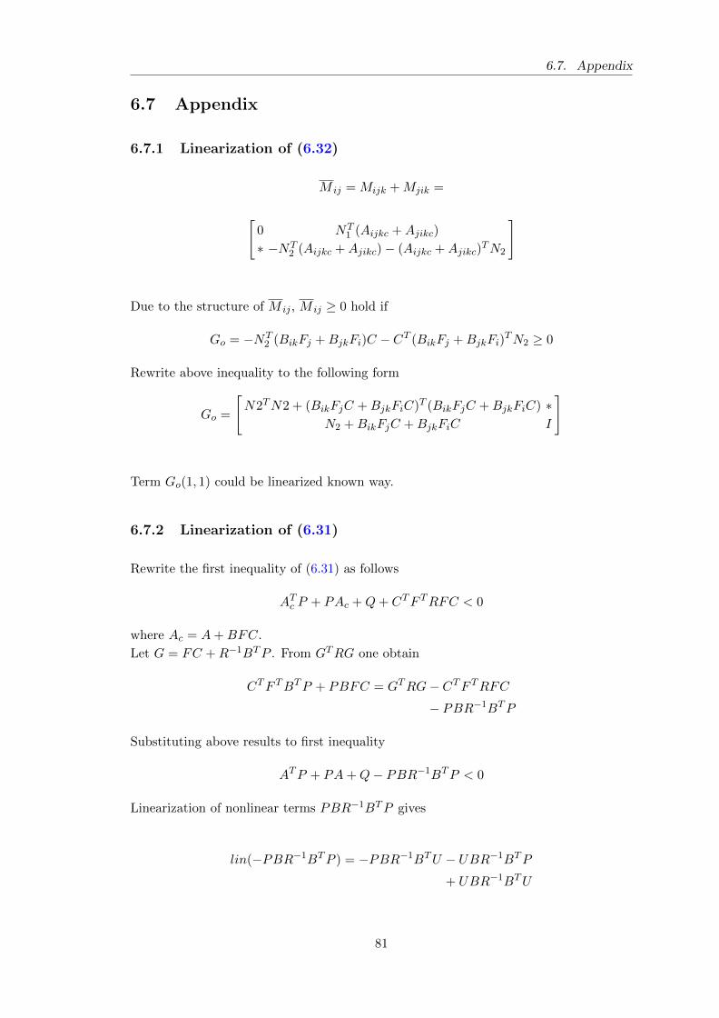
6.7. Appendix
6.7 Appendix
6.7.1 Linearization of (6.32)
M ij = Mijk +Mjik =
[0 NT
1 (Aijkc +Ajikc)
∗ −NT2 (Aijkc +Ajikc)− (Aijkc +Ajikc)
TN2
]
Due to the structure of M ij , M ij ≥ 0 hold if
Go = −NT2 (BikFj +BjkFi)C − CT (BikFj +BjkFi)
TN2 ≥ 0
Rewrite above inequality to the following form
Go =
[N2TN2 + (BikFjC +BjkFiC)T (BikFjC +BjkFiC) ∗
N2 +BikFjC +BjkFiC I
]
Term Go(1, 1) could be linearized known way.
6.7.2 Linearization of (6.31)
Rewrite the first inequality of (6.31) as follows
ATc P + PAc +Q+ CTF TRFC < 0
where Ac = A+BFC.
Let G = FC +R−1BTP . From GTRG one obtain
CTF TBTP + PBFC = GTRG− CTF TRFC− PBR−1BTP
Substituting above results to first inequality
ATP + PA+Q− PBR−1BTP < 0
Linearization of nonlinear terms PBR−1BTP gives
lin(−PBR−1BTP ) = −PBR−1BTU − UBR−1BTP
+ UBR−1BTU
81
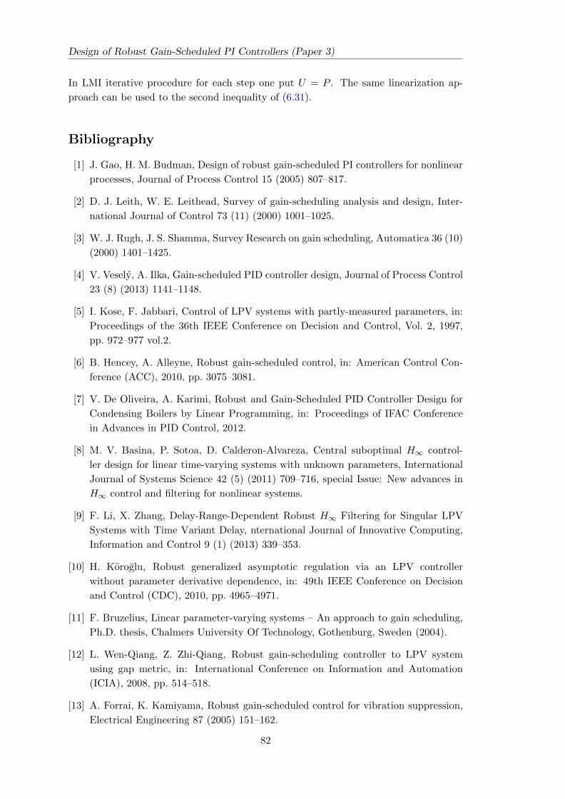
Design of Robust Gain-Scheduled PI Controllers (Paper 3)
In LMI iterative procedure for each step one put U = P . The same linearization ap-
proach can be used to the second inequality of (6.31).
Bibliography
[1] J. Gao, H. M. Budman, Design of robust gain-scheduled PI controllers for nonlinear
processes, Journal of Process Control 15 (2005) 807–817.
[2] D. J. Leith, W. E. Leithead, Survey of gain-scheduling analysis and design, Inter-
national Journal of Control 73 (11) (2000) 1001–1025.
[3] W. J. Rugh, J. S. Shamma, Survey Research on gain scheduling, Automatica 36 (10)
(2000) 1401–1425.
[4] V. Vesely, A. Ilka, Gain-scheduled PID controller design, Journal of Process Control
23 (8) (2013) 1141–1148.
[5] I. Kose, F. Jabbari, Control of LPV systems with partly-measured parameters, in:
Proceedings of the 36th IEEE Conference on Decision and Control, Vol. 2, 1997,
pp. 972–977 vol.2.
[6] B. Hencey, A. Alleyne, Robust gain-scheduled control, in: American Control Con-
ference (ACC), 2010, pp. 3075–3081.
[7] V. De Oliveira, A. Karimi, Robust and Gain-Scheduled PID Controller Design for
Condensing Boilers by Linear Programming, in: Proceedings of IFAC Conference
in Advances in PID Control, 2012.
[8] M. V. Basina, P. Sotoa, D. Calderon-Alvareza, Central suboptimal H∞ control-
ler design for linear time-varying systems with unknown parameters, International
Journal of Systems Science 42 (5) (2011) 709–716, special Issue: New advances in
H∞ control and filtering for nonlinear systems.
[9] F. Li, X. Zhang, Delay-Range-Dependent Robust H∞ Filtering for Singular LPV
Systems with Time Variant Delay, nternational Journal of Innovative Computing,
Information and Control 9 (1) (2013) 339–353.
[10] H. Koroglu, Robust generalized asymptotic regulation via an LPV controller
without parameter derivative dependence, in: 49th IEEE Conference on Decision
and Control (CDC), 2010, pp. 4965–4971.
[11] F. Bruzelius, Linear parameter-varying systems – An approach to gain scheduling,
Ph.D. thesis, Chalmers University Of Technology, Gothenburg, Sweden (2004).
[12] L. Wen-Qiang, Z. Zhi-Qiang, Robust gain-scheduling controller to LPV system
using gap metric, in: International Conference on Information and Automation
(ICIA), 2008, pp. 514–518.
[13] A. Forrai, K. Kamiyama, Robust gain-scheduled control for vibration suppression,
Electrical Engineering 87 (2005) 151–162.
82
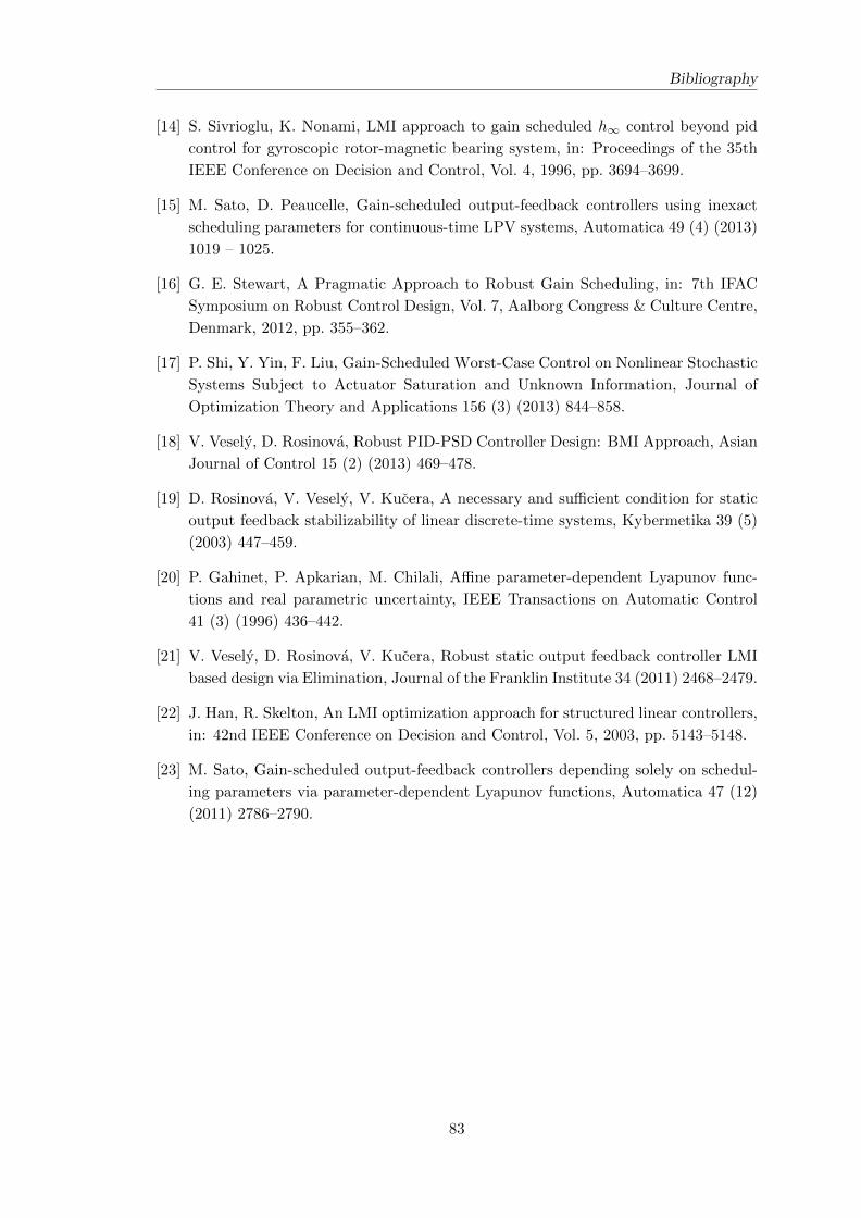
Bibliography
[14] S. Sivrioglu, K. Nonami, LMI approach to gain scheduled h∞ control beyond pid
control for gyroscopic rotor-magnetic bearing system, in: Proceedings of the 35th
IEEE Conference on Decision and Control, Vol. 4, 1996, pp. 3694–3699.
[15] M. Sato, D. Peaucelle, Gain-scheduled output-feedback controllers using inexact
scheduling parameters for continuous-time LPV systems, Automatica 49 (4) (2013)
1019 – 1025.
[16] G. E. Stewart, A Pragmatic Approach to Robust Gain Scheduling, in: 7th IFAC
Symposium on Robust Control Design, Vol. 7, Aalborg Congress & Culture Centre,
Denmark, 2012, pp. 355–362.
[17] P. Shi, Y. Yin, F. Liu, Gain-Scheduled Worst-Case Control on Nonlinear Stochastic
Systems Subject to Actuator Saturation and Unknown Information, Journal of
Optimization Theory and Applications 156 (3) (2013) 844–858.
[18] V. Vesely, D. Rosinova, Robust PID-PSD Controller Design: BMI Approach, Asian
Journal of Control 15 (2) (2013) 469–478.
[19] D. Rosinova, V. Vesely, V. Kucera, A necessary and sufficient condition for static
output feedback stabilizability of linear discrete-time systems, Kybermetika 39 (5)
(2003) 447–459.
[20] P. Gahinet, P. Apkarian, M. Chilali, Affine parameter-dependent Lyapunov func-
tions and real parametric uncertainty, IEEE Transactions on Automatic Control
41 (3) (1996) 436–442.
[21] V. Vesely, D. Rosinova, V. Kucera, Robust static output feedback controller LMI
based design via Elimination, Journal of the Franklin Institute 34 (2011) 2468–2479.
[22] J. Han, R. Skelton, An LMI optimization approach for structured linear controllers,
in: 42nd IEEE Conference on Decision and Control, Vol. 5, 2003, pp. 5143–5148.
[23] M. Sato, Gain-scheduled output-feedback controllers depending solely on schedul-
ing parameters via parameter-dependent Lyapunov functions, Automatica 47 (12)
(2011) 2786–2790.
83

7
Robust Gain-scheduled PID Controller
Design for uncertain LPV systems
(Paper 4)
Abstract
A novel methodology is proposed for robust gain-scheduled PID controller design for
uncertain LPV systems. The proposed design procedure is based on the parameter-
dependent quadratic stability approach. A new uncertain LPV system model has been
introduced in this paper. To access the performance quality the approach of a parameter
varying guaranteed cost is used which allowed to reach for different working points
desired performance. Numerical examples show the benefit of the proposed method.
Keywords: LPV systems, Gain-scheduled controller, Robust controller, Parameter-
dependent Lyapunov function, Quadratic gain-scheduled cost function, PID controller.
7.1 Introduction
In real applications a controller must accommodate a plant with changing dynamics.
Therefore, controllers based on these models have to be robust in the presence of plant
model uncertainty. A practical approach involves scheduling in a family of local con-
trollers in response to the changing plant dynamics [1]. A proposed family of local
controllers is implemented using the gain scheduling approach. The above mentioned
gain-scheduled designs are guided by two heuristic rules [2]:
– the scheduling variable should vary slowly, and
– the scheduling variable should capture the plants nonlinearities.
85
Robust GS PID Controller Design for uncertain LPV systems (Paper 4)
In such cases, the designed gain-scheduled controller should be able to stabilize and
guarantee a reasonable performance for all operating conditions. The question remains
what happens with a closed-loop system if the developed physical nonlinear model or
the model obtained through practical identification is not enough precise? In such a
case, frequent in applications, there is a need for robust controller to cope with plant
model uncertainty.
Various robust controller design methods for gain-scheduled uncertain plant are avail-
able in literature. Robust gain-scheduled controllers design to LPV system can be found
in [1], where the authors addressed the problem of interpolating in a set of LTI control-
lers in order to form a gain-scheduled controller with optimal H∞ performance. The
set of admissible interpolated controllers are framed in terms of the robust controller
interpolation criteria. For a special uncertain dynamical system, the robust state feed-
back stabilization problem in the gain scheduling can be found in [3]. In this paper it
is shown that a possible advantage of the online measurement of the scheduling para-
meters is that this always allows linear compensators, whose implementation can be
easier than that of nonlinear ones. Design of robust gain-scheduled PI controllers for
nonlinear SISO process can be found in [2]. The model uncertainty is assumed to be the
difference between the nonlinear model and the linear one. In the paper [4] an input-
output approach to the gain-scheduled design of nonlinear controllers is presented. A
controller formulation inspired by the Youla-Kucera parametrization to propose a con-
troller structure and design approach that allow the gain scheduling of linear control
designs such that a robustly stable nonlinear closed-loop control system is achieved. A
robust PID controller is designed in [5].The main feature of the proposed method is that
the stability, robustness margin and some performance specification are guaranteed by
linear constraints in the Nyquist diagram. The condensing boiler is described by the
first order model with a time delay in [6], the problem of attenuation of sinusoidal dis-
turbances with uncertain and arbitrarily time-varying frequencies is solved by synthesis
of LPV controller using the L2 gain method. In [7] the quadratic stability approach is
used to design the gain-scheduled controller for each vertex of a plant uncertainty box
and the closed-loop system stability is verified by LMI. Other alternative approaches to
gain-scheduled controller design can be found in [8], [9], [10], [11], [12], [13], [14], [15],
[16], [17]. A survey of the gain-scheduled controller design is given in excellent papers
[18] and [19].
The above short survey implies that in the references there is no systematic procedure
for designing a robust PID gain-scheduled controller. This observation motivated us
to solve the following research problem: design a PID robust gain-scheduled controller
which should guarantee
– stability and robustness properties of a closed-loop system for all scheduled para-
meters θ ∈ Ωs and their rate θi ∈ Ωt, when the uncertain plant parameters π lie
in the given polytopic uncertainty box Ω, that is π ∈ Ω, θ ∈ Ωs, θ ∈ Ωt,
– for the closed-loop system ensure for all π ∈ Ω, θ ∈ Ωs and θ ∈ Ωt guaranteed
gain-scheduled performance and parameter dependent quadratic stability.
86
7.2. Problem formulation and preliminaries
In this paper the new PID robust gain-scheduled controller design procedure is given.
The paper is organized as follows. Section 7.2 includes problem formulation of robust
PID gain-scheduled controllers design for the original plant uncertainty model and new
performance criterion. In Section 7.3, sufficient robust stability LMI conditions for
the structured gain-scheduled controller are given. Respective conditions for robust
controller synthesis are in BMI form. In Section 7.4, the results are illustrated on
examples to design a PID robust gain-scheduled controller. The final Section 7.5 brings a
conclusion on the obtained results and possible directions in the gain-scheduled controller
design field.
Hereafter, the following notational convention will be adopted. Given a symmetric mat-
rix P = P T ∈ Rn×n, the inequality P > 0 (P ≥ 0) denotes the positive definiteness
(semidefiniteness) matrix. Symbol ∗ denotes a block that is transposed and complex con-
jugated to the respective symmetrically placed one. Matrices, if not explicitly stated, are
assumed to have compatible dimensions. I denotes the identity matrix of corresponding
dimensions.
7.2 Problem formulation and preliminaries
Consider a continuous-time linear parameter varying (LPV) uncertain system in the
form
x = A(ξ, θ)x+B(ξ, θ)u
y = Cx
yd = Cdx
(7.1)
where linear parameter varying matrices
A(ξ, θ) = A0(ξ) +
s∑i=1
Ai(ξ)θi ∈ Rn×n
B(ξ, θ) = B0(ξ) +
s∑i=1
Bi(ξ)θi ∈ Rn×m(7.2)
x ∈ Rn, u ∈ Rm, y ∈ Rl denote the state, control input and controlled output, respect-
ively. Matrices Ai(ξ), Bi(ξ), i = 0, 1, 2, . . . , s belong to the convex set: a polytope with
N vertices that can be formally defined as
Ω =
Ai(ξ), Bi(ξ) =
N∑j=1
(Aij , Bij) ξj
,
i = 0, 1, 2, . . . , s,
N∑j=1
ξj = 1, ξj ≥ 0
(7.3)
87
Robust GS PID Controller Design for uncertain LPV systems (Paper 4)
where s is the number of scheduled parameters; ξj , j = 1, 2, . . . , N are constant or
possibly time varying but unknown parameters; matrices Aij , Bij , C, Cd are constant
matrices of corresponding dimensions, where Cd is the output matrix for D part of
the controller. θ ∈ Rs is a vector of known (measurable) constant or possibly time-
varying scheduled parameters. Assume that both lower and upper bounds are available.
Specifically
1. Each parameter θi, i = 1, 2, . . . , s ranges between known extremal values
θ ∈ Ωs =θ ∈ Rs : θi ∈ 〈θi, θi〉, i = 1, 2, . . . , s
(7.4)
2. The rate of variation θi is well defined at all times and satisfies
θ ∈ Ωt =θi ∈ Rs : θi ∈ 〈θi, θi〉, i = 1, 2, . . . , s
(7.5)
Note that system (7.1), (7.2), (7.3) consists of two type of vertices. The first one is due
to the gain-scheduled parameters θ with T = 2s vertices – θ vertices, and the second
set of vertices are due to uncertainties of the system – N , ξ vertices. For robust gain-
scheduled ”I” part controller design the states of system (7.1) need to be extended in
such a way that a static output feedback control algorithm can provide proportional (P)
and integral (I) parts of the designed controller. For more details see [20]. Assume that
system (7.1) allows PI controller design with a static output feedback.
To access the system performance, we consider an original scheduling quadratic cost
function
J =
∫ ∞0
J(t)dt =
∫ ∞0
(xTQ(θ)x+ uTRu+ xTS(θ)x
)dt (7.6)
where
Q(θ) = Q0 +s∑i=1
Qiθi, S(θ) = S0 +s∑i=1
Siθi
The feedback control law is considered in the form
u = F (θ)y + Fd(θ)yd (7.7)
where
F (θ) = F0 +s∑i=1
Fiθi, Fd(θ) = Fd0 +s∑i=1
Fdiθi
Matrices Fi, Fdi, i = 0, 1, 2, . . . , s are the static output PI part and the output deriv-
ative feedback gain-scheduled controller. The structure of the above matrices can be
prescribed.
The respective closed-loop system is then
Md(ξ, θ)x = Ac(ξ, θ)x (7.8)
88
7.2. Problem formulation and preliminaries
where
Md(ξ, θ) = I −B(ξ, θ)Fd(θ)Cd
Ac(ξ, θ) = A(ξ, θ) +B(ξ, θ)F (θ)C
Let as recall some results about an optimal control of time varying systems [21].
Lemma 7.1. Let there exists a scalar positive definite function V (x, t) such that
limt→∞ V (x, t) = 0 which satisfies
minu∈Ωu
δV
δxAc(θ) +
δV
δt+ J(t)
= 0 (7.9)
From (7.9) obtained control algorithm u = u∗(x, t) ensure the closed-loop stability and
on the solution of (7.1) optimal value of cost function as J∗ = J(x0, t0) = V (x(0), t0).
Eq. (7.9) is known as Bellman-Lyapunov equation and function V (x, t) which satisfies
to (7.9) is Lyapunov function. For a given concrete structure of Lyapunov function the
optimal control algorithm may reduces from ”if and only if ” to ”if ” and for switched
systems, robust control, gain-scheduled control and so on to guaranteed cost.
Definition 7.1. Consider a stable closed-loop system (7.8). If there exists a control law
u (7.7) which satisfies (7.11) and a positive scalar J∗ such that the value of closed-loop
cost function (7.6) J satisfies J < J∗ for all θ ∈ Ωs and ξj , j = 1, 2 . . . , N satisfying
(7.3), then J∗ is said to be a guaranteed cost and u is said to be a guaranteed cost
control law for system (7.8).
Let us recall some parameter dependent stability results which provide basic further
developments.
Definition 7.2. Closed-loop system (7.8) is parameter dependent quadratically stable
in the convex domain Ω given by (7.3) for all θ ∈ Ωs and θ ∈ Ωt if and only if there
exists a positive definite parameter dependent Lyapunov function V (ξ, θ) such that the
time derivative of Lyapunov function with respect to (7.8) is
dV (ξ, θ, t)
dt< 0 (7.10)
Lemma 7.2. Consider the closed-loop system (7.8). Control algorithm (7.7) is the
guaranteed cost control law if and only if there exists a parameter dependent Lyapunov
function V (ξ, θ) such that the following condition holds [21]
Be(ξ, θ) = minu
(dV (ξ, θ, t)
dt+ J(t)
)≤ 0 (7.11)
Uncertain closed-loop system (7.8) conforming to Lemma 7.2 is called robust parameter
dependent quadratically stable with guaranteed cost.
We proceed with the notion of multi-convexity of a scalar quadratic function [22].
89
Robust GS PID Controller Design for uncertain LPV systems (Paper 4)
Lemma 7.3. Consider a scalar quadratic function of θ ∈ Rs
f(θ) = α0 +
s∑i=1
αiθi +
s∑i=1
s∑j>i
βijθiθj +
s∑i=1
γiθ2i (7.12)
and assume that if f(θ) is multiconvex that is
∂2f
∂θ2i
= 2γi ≥ 0, i = 1, 2, . . . , s
Then f(θ) is negative in the hyper rectangle (7.4) if and only if it takes negative values
at the vertices of (7.4), that is if and only if f(θ) < 0 for all vertices of the set given by
(7.4). For decrease the conservatism of Lemma 7.3 the approach proposed in [22] can be
used.
In this paragraph for uncertain gain scheduling system (7.1) we have proposed to use a
model uncertainty in the form of a convex set with N vertices defined by (7.3). Further-
more, we consider the new type of performance (7.6) to obtain the closed-loop system
guaranteed cost.
7.3 Main Results
This section formulates the theoretical approach to robust PID gain-scheduled con-
troller design for polytopic system (7.1), (7.2), (7.3) which ensures closed-loop system
parameter dependent quadratic stability and a guaranteed cost for all gain scheduling
parameters θ ∈ Ωs, and θ ∈ Ωt. The main result on robust stability for the gain-
scheduled control system is given in the next theorem.
Theorem 7.1. The closed-loop system (7.8) is robust parameter dependent quadratic-
ally stable with a guaranteed cost if there exist positive definite matrix P (ξ, θ) ∈ Rn×n,
matrices N1, N2 ∈ Rn×n positive definite (semidefinite) matrices Q(θ), R, S(θ) and
gain-scheduled controller (7.7) such that
a)
L(ξ, θ) = W0(ξ) +s∑i=1
Wi(ξ)θi+
+s∑i=1
s∑j>i
Wij(ξ)θiθj +
s∑i=1
Wiiθ2i < 0
(7.13)
b)
Wii(ξ) ≥ 0, θ ∈ Ωs, i = 1, 2, . . . , s (7.14)
90
7.3. Main Results
where we consider parameter dependent Lyapunov matrix
P (ξ, θ) = P0(ξ) +
s∑i=1
Pi(ξ)θi > 0 (7.15)
the above matrices (7.13) and (7.14) are given as follows:
W0(ξ) =
[W110(ξ) W120(ξ)
∗ W220(ξ)
]W110(ξ) = S0 + CTd Fd
T0 RFd0Cd
+NT1 (I −B0(ξ)Fd0Cd)
+ (I −B0(ξ)Fd0Cd)T N1
W120(ξ) = −NT1 (A0(ξ) +B0(ξ)F0C)
+ (I −B0(ξ)Fd0Cd)T N2 + P0(ξ)
+CTd FdT0 RF0C
W220(ξ) = −NT2 (A0(ξ) +B0(ξ)F0C)
− (A0(ξ) +B0(ξ)F0C)T N2 +Q0
+CTF T0 RF0C +∑s
j=1 Pj(ξ)θi
Wi(ξ) =
[W11i(ξ) W12i(ξ)
∗ W22i(ξ)
]W11i(ξ) = Si + CTd
(Fd
T0 RFdi + Fd
Ti RFd0
)Cd
−NT1 (B0(ξ)Fdi +Bi(ξ)Fd0)Cd
− [(B0(ξ)Fdi +Bi(ξ)Fd0)Cd]T N1
W12i(ξ) = −NT1 (Ai(ξ) +B0(ξ)Fi +Bi(ξ)F0)C
− (Bi(ξ)Fd0Cd)T N2 + Pi(ξ)
+CTd(Fd
Ti RF0 + Fd
T0 RFi
)C
W22i(ξ) = −NT2 (Ai(ξ) + (B0(ξ)Fi +Bi(ξ)F0)C)
− [Ai(ξ) + (B0(ξ)Fi +Bi(ξ)F0)C]T N2
+Qi + CT(F T0 RFi + F Ti RF0
)C
Wij(ξ) =
[W11ij(ξ) W12ij(ξ)
∗ W22ij(ξ)
]W11ij(ξ) = CTd
(Fd
Ti RFdj + Fd
Tj RFdi
)Cd
−NT1
(Bi(ξ)Fdj +Bj(ξ)Fdi
)Cd
−CTd(Bi(ξ)Fdj +Bj(ξ)Fdi
)TN1
W12ij(ξ) = −NT1 (Bi(ξ)Fj +Bj(ξ)Fi)C
−CTd(Bi(ξ)Fdj +Bj(ξ)Fdi
)TN2
+CTd(Fd
Ti RFj + Fd
Tj RFi
)C
W22ij(ξ) = −NT2 (Bi(ξ)Fj +Bj(ξ)Fi)C
−CT (Bi(ξ)Fj +Bj(ξ)Fi)T N2
+CT(F Ti RFj + F Tj RFi
)C
Wii(ξ) =
[W11ii(ξ) W12ii(ξ)
∗ W22ii(ξ)
]W11ii(ξ) = CTd Fd
Ti RFdiCd −NT
1 Bi(ξ)FdiCd−CTd FdTi Bi(ξ)TN1
91
Robust GS PID Controller Design for uncertain LPV systems (Paper 4)
W12ii(ξ) = −NT1 Bi(ξ)FiC − CTd FdTi BT
i (ξ)N2
+CTd FdTi RFiC
W22ii(ξ) = −NT2 Bi(ξ)FiC − CTF Ti BT
i (ξ)N2
+CTF Ti RFiC
Due to space we provide only the outline of the proof. The proof is based on Lemma
7.2 and 7.3. The time derivative of the Lyapunov function V (ξ, θ) = xTP (ξ, θ)x is
dV (ξ, θ)
dt=[xT xT
] [ 0 P (ξ, θ)
P (ξ, θ) P (ξ, θ)
][x
x
](7.16)
where
P (ξ, θ) =s∑i=1
Pi(ξ)θ
To isolate two matrices (system and Lyapunov) introducing matrices N1, N2 in the
following way
[2N1x+ 2N2x]T [Md(ξθ)x−Ac(ξ, θ)] = 0 (7.17)
and substituting (7.17), (7.16), J(t) (7.6) and control law (7.7) to (7.11), after some
manipulation one obtains
Be(ξ, θ) =[xT xT
] [ W11(ξ) W12(ξ)
W12T (ξ) W22(ξ)
][x
x
](7.18)
whereW11 = S(θ) + CTd F
Td (θ)RFd(θ)Cd +NT
1 Md(ξ, θ)
+MTd (ξ, θ)N1
W12 = −NT1 Ac(ξ, θ) +MT
d (ξ, θ)N2 + P (ξ, θ)
+CTd FTd (θ)RF (θ)C
W22 = −NT2 Ac(ξ, θ)−ATc (ξ, θ)N2 +Q(θ)
+CTF T (θ)RF (θ)C + P (ξ, θ)
Eq. (7.18) immediately implies (7.13), which proves the sufficient conditions of The-
orem 7.1.
Eq.’s (7.13) and (7.14) are linear with respect to uncertain parameter ξj , j = 1, 2, . . . , N ,
therefore (7.13) and (7.14) have to hold for all j = 1, 2, . . . , N . For the known gain-
scheduled controller parameters, inequalities (7.13) and (7.14) reduce to LMI, for gain-
scheduled controller synthesis problem (7.13) (7.14) are BMI.
Remark 7.1. Theorem 7.1 can be used for a quadratic stability test, where Lyapuunov
function matrices (matrix) are either independent of parameter ξj , j = 1, 2, . . . , N or
parameter θi, i = 1, 2, . . . , s or both as listed below.
1. Quadratic stability with respect to model parameter variation. For this case one
has P (θ) = P0 +∑s
i=1 Piθi. This Lyapunov function should withstand arbitrarily
fast model parameter variation in the convex set (7.3)
92
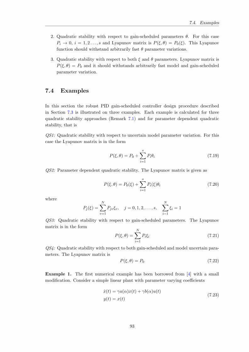
7.4. Examples
2. Quadratic stability with respect to gain-scheduled parameters θ. For this case
Pi → 0, i = 1, 2 . . . , s and Lyapunov matrix is P (ξ, θ) = P0(ξ). This Lyapunov
function should withstand arbitrarily fast θ parameter variations.
3. Quadratic stability with respect to both ξ and θ parameters. Lyapunov matrix is
P (ξ, θ) = P0 and it should withstands arbitrarily fast model and gain-scheduled
parameter variation.
7.4 Examples
In this section the robust PID gain-scheduled controller design procedure described
in Section 7.3 is illustrated on three examples. Each example is calculated for three
quadratic stability approaches (Remark 7.1) and for parameter dependent quadratic
stability, that is
QS1: Quadratic stability with respect to uncertain model parameter variation. For this
case the Lyapunov matrix is in the form
P (ξ, θ) = P0 +s∑i=1
Piθi (7.19)
QS2: Parameter dependent quadratic stability. The Lyapunov matrix is given as
P (ξ, θ) = P0(ξ) +s∑i=1
Pi(ξ)θi (7.20)
where
Pj(ξ) =N∑v=1
Pjvξv, j = 0, 1, 2, . . . , s,N∑i=1
ξi = 1
QS3: Quadratic stability with respect to gain-scheduled parameters. The Lyapunov
matrix is in the form
P (ξ, θ) =
N∑i=1
Piξi (7.21)
QS4: Quadratic stability with respect to both gain-scheduled and model uncertain para-
meters. The Lyapunov matrix is
P (ξ, θ) = P0 (7.22)
Example 1. The first numerical example has been borrowed from [4] with a small
modification. Consider a simple linear plant with parameter varying coefficients
x(t) = γa(α)x(t) + γb(α)u(t)
y(t) = x(t)(7.23)
93
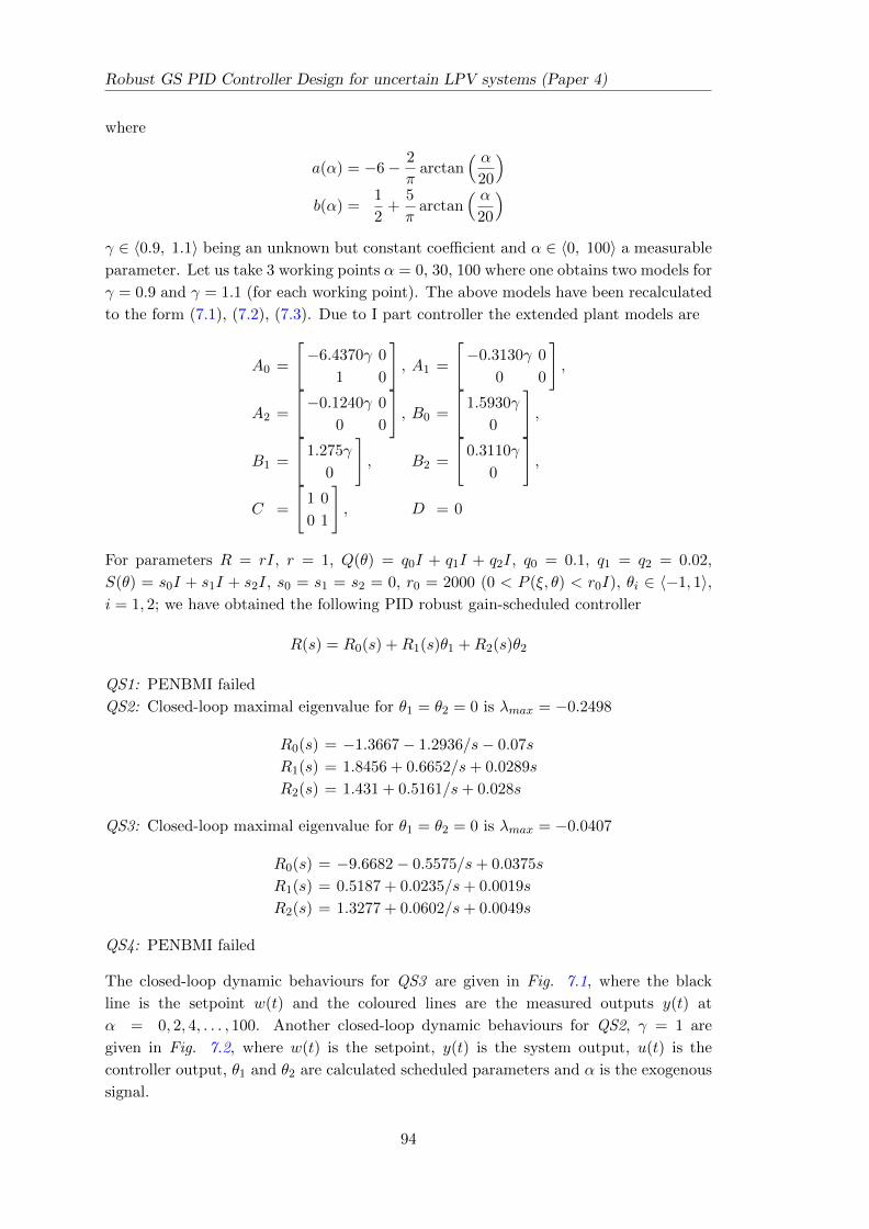
Robust GS PID Controller Design for uncertain LPV systems (Paper 4)
where
a(α) = −6− 2
πarctan
( α20
)b(α) =
1
2+
5
πarctan
( α20
)γ ∈ 〈0.9, 1.1〉 being an unknown but constant coefficient and α ∈ 〈0, 100〉 a measurable
parameter. Let us take 3 working points α = 0, 30, 100 where one obtains two models for
γ = 0.9 and γ = 1.1 (for each working point). The above models have been recalculated
to the form (7.1), (7.2), (7.3). Due to I part controller the extended plant models are
A0 =
[−6.4370γ 0
1 0
], A1 =
[−0.3130γ 0
0 0
],
A2 =
[−0.1240γ 0
0 0
], B0 =
[1.5930γ
0
],
B1 =
[1.275γ
0
], B2 =
[0.3110γ
0
],
C =
[1 0
0 1
], D = 0
For parameters R = rI, r = 1, Q(θ) = q0I + q1I + q2I, q0 = 0.1, q1 = q2 = 0.02,
S(θ) = s0I + s1I + s2I, s0 = s1 = s2 = 0, r0 = 2000 (0 < P (ξ, θ) < r0I), θi ∈ 〈−1, 1〉,i = 1, 2; we have obtained the following PID robust gain-scheduled controller
R(s) = R0(s) +R1(s)θ1 +R2(s)θ2
QS1: PENBMI failed
QS2: Closed-loop maximal eigenvalue for θ1 = θ2 = 0 is λmax = −0.2498
R0(s) = −1.3667− 1.2936/s− 0.07s
R1(s) = 1.8456 + 0.6652/s+ 0.0289s
R2(s) = 1.431 + 0.5161/s+ 0.028s
QS3: Closed-loop maximal eigenvalue for θ1 = θ2 = 0 is λmax = −0.0407
R0(s) = −9.6682− 0.5575/s+ 0.0375s
R1(s) = 0.5187 + 0.0235/s+ 0.0019s
R2(s) = 1.3277 + 0.0602/s+ 0.0049s
QS4: PENBMI failed
The closed-loop dynamic behaviours for QS3 are given in Fig. 7.1, where the black
line is the setpoint w(t) and the coloured lines are the measured outputs y(t) at
α = 0, 2, 4, . . . , 100. Another closed-loop dynamic behaviours for QS2, γ = 1 are
given in Fig. 7.2, where w(t) is the setpoint, y(t) is the system output, u(t) is the
controller output, θ1 and θ2 are calculated scheduled parameters and α is the exogenous
signal.
94
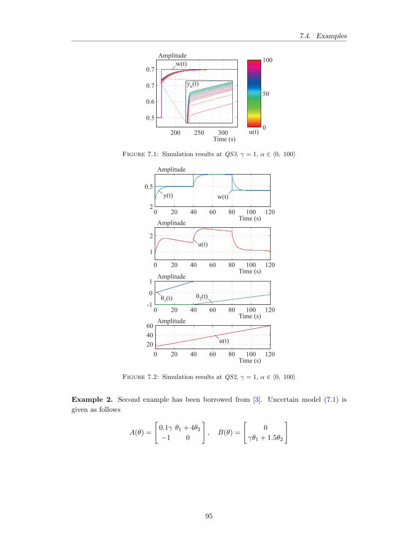
7.4. Examples
Figure 7.1: Simulation results at QS3, γ = 1, α ∈ 〈0, 100〉
Figure 7.2: Simulation results at QS2, γ = 1, α ∈ 〈0, 100〉
Example 2. Second example has been borrowed from [3]. Uncertain model (7.1) is
given as follows
A(θ) =
[0.1γ θ1 + 4θ2
−1 0
], B(θ) =
[0
γθ1 + 1.5θ2
]
95
Robust GS PID Controller Design for uncertain LPV systems (Paper 4)
where θ1 + θ2 = 1, θi ≥ 0, i = 1, 2 and uncertain parameter γ ∈ 〈0.9, 1.1〉. Substituting
for θ2 = 1− θ1 and for γ = 0.9 or γ = 1.1 one obtains
A01 =
[0.09 4
−1 0
], A02 =
[0.11 4
−1 0
],
A11 = A12 =
[0 −3
0 0
], B01 = B02 =
[0
1.5
],
B11 =
[0
−0.6
], B12 =
[0
−0.4
],
C =[
1 1], D = 0
For parameters r = 1, θ1 ∈ 〈0, 1〉, q0 = 0.001, s0 = 0, q1 = 0.0002, s1 = 0, r0 = 20000
the following PID controller is obtained
QS1: Closed-loop maximal eigenvalue for θ1 = θ2 = 0 is λmax = −0.1483
R0(s) = −4.2735− 0.7288/s− 0.521s
R1(s) = −29.0575− 8.6869/s− 15.9056s
QS2: PENBMI failed
QS3: Closed-loop maximal eigenvalue for θ1 = θ2 = 0 is λmax = −0.1129
R0(s) = 0.0805− 0.0466/s− 1.9234s
R1(s) = −0.0649− 0.4289/s− 15.0506s
QS4: Closed-loop maximal eigenvalue for θ1 = θ2 = 0 is λmax = −0.0752
R0(s) = 0.0304− 0.0405/s− 1.7515s
R1(s) = −0.0763− 0.5508/s− 19.9456
The closed-loop dynamic behaviours are given in Fig. 7.3.
Example 3. Consider the uncertain system (7.1) [9]
A0 =
[0.2γ −0.8
0.3 −1.3
], A1 =
[0.0 −0.3γ
0.5γ 0
],
B0 =
[0.4
0.8γ
], B1 =
[0.3
0.1
]γ, C =
[1 0]
where γ ∈ 〈0.9, 1.1〉 constant but uncertain parameter θ1 ∈ 〈0, 1〉. Despite the simplicity
the system with state feedback is not quadratically stabilizable with a fixed gain matrix
for γ = 1. Substituting γ = 0.9 and γ = 1.1 we obtain the uncertain plant model (7.1).
For parameters r = 1, q0 = 0.0001, s0 = 0, q1 = 0.0001, s1 = 0 and r0 = 20000 the
following robust PID controllers are obtained
QS1: Closed-loop maximal eigenvalue for θ1 = θ2 = 0 is λmax = −0.0222
R0(s) = 1.0149 + 0.0172/s− 1.94333s
R1(s) = [−0.4446 + 0.6918/s+ 11.845s]× 10−14 .= 0
96
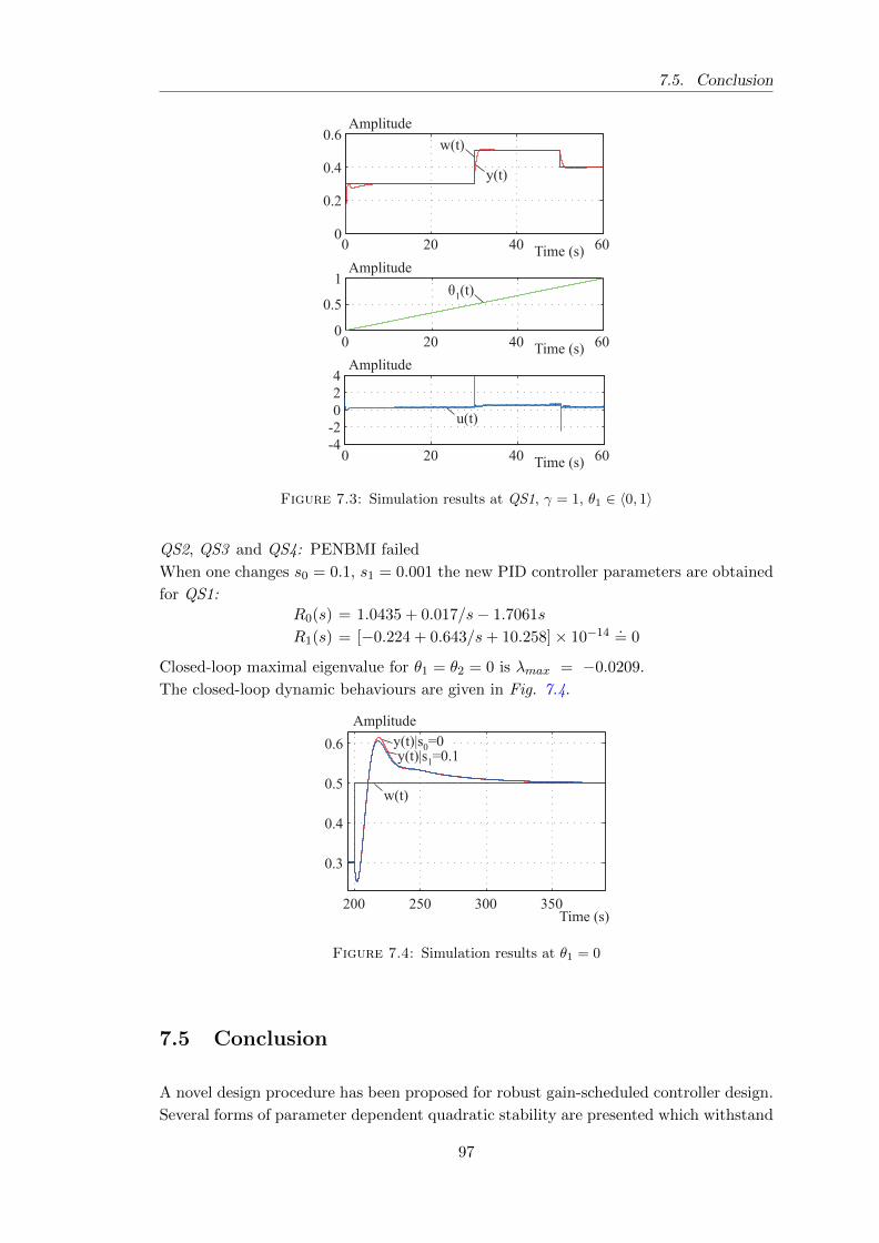
7.5. Conclusion
Figure 7.3: Simulation results at QS1, γ = 1, θ1 ∈ 〈0, 1〉
QS2, QS3 and QS4: PENBMI failed
When one changes s0 = 0.1, s1 = 0.001 the new PID controller parameters are obtained
for QS1:
R0(s) = 1.0435 + 0.017/s− 1.7061s
R1(s) = [−0.224 + 0.643/s+ 10.258]× 10−14 .= 0
Closed-loop maximal eigenvalue for θ1 = θ2 = 0 is λmax = −0.0209.
The closed-loop dynamic behaviours are given in Fig. 7.4.
Figure 7.4: Simulation results at θ1 = 0
7.5 Conclusion
A novel design procedure has been proposed for robust gain-scheduled controller design.
Several forms of parameter dependent quadratic stability are presented which withstand
97
Robust GS PID Controller Design for uncertain LPV systems (Paper 4)
arbitrarily fast model parameter variation or/and arbitrarily fast gain-scheduled para-
meter variation. Because of BMI approach the future research should transform BMI
to LMI and the obtained design procedure for a polytopic continuous system should be
transformed to discrete ones. The proposed approach contributes to the design tools of
a robust gain-scheduled controller for uncertain polytopic systems.
Bibliography
[1] B. Hencey, A. Alleyne, Robust gain-scheduled control, in: American Control Con-
ference (ACC), 2010, pp. 3075–3081.
[2] J. Gao, H. M. Budman, Design of robust gain-scheduled PI controllers for nonlinear
processes, Journal of Process Control 15 (7) (2005) 807–817.
[3] F. Blanchini, The gain scheduling and the robust state feedback stabilization prob-
lems, IEEE Transactions on Automatic Control 45 (11) (2000) 2061–2070.
[4] G. E. Stewart, A Pragmatic Approach to Robust Gain Scheduling, in: 7th IFAC
Symposium on Robust Control Design, Vol. 7, Aalborg Congress & Culture Centre,
Denmark, 2012, pp. 355–362.
[5] V. De Oliveira, A. Karimi, Robust and Gain-Scheduled PID Controller Design for
Condensing Boilers by Linear Programming, in: Proceedings of IFAC Conference
in Advances in PID Control, 2012.
[6] H. Koroglu, Robust generalized asymptotic regulation via an LPV controller
without parameter derivative dependence, in: 49th IEEE Conference on Decision
and Control (CDC), 2010, pp. 4965–4971.
[7] A. Forrai, K. Kamiyama, Robust gain-scheduled control for vibration suppression,
Electrical Engineering 87 (3) (2005) 151–162.
[8] F. Wang, V. Balakrishnan, Improved stability analysis and gain-scheduled control-
ler synthesis for parameter-dependent systems, IEEE Transactions on Automatic
Control 47 (5) (2002) 720–734.
[9] V. F. Montagner, P. L. D. Peres, State feedback gain scheduling for linear sys-
tems with time-varying parameters, in: Proceedings of the 2004 American Control
Conference, Vol. 3, 2004, pp. 2004–2009.
[10] P. Apkarian, P. Gahinet, G. Becker, Self-Scheduled H∞ Control of Linear
Parameter-Varying Systems: A Design Example, Automatica 31 (9) (1995) 1251–
1261.
[11] F. D. Adegas, J. Stoustrup, Structured control of affine linear parameter varying
systems, in: American Control Conference (ACC), 2011, pp. 739–744.
[12] L. Wen-Qiang, Z. Zhi-Qiang, Robust gain-scheduling controller to LPV system
using gap metric, in: International Conference on Information and Automation
(ICIA), 2008, pp. 514–518.
98
Bibliography
[13] M. S. Spillman, P. A. Blue, L. H. Lee, S. S. Banda, A Robust Gain-Scheduling
Example User Linear Parameter-Varying Feedback, in: Proceedings of the IFAC
13 th Triennial World Congress, 1996, pp. 221–226.
[14] V. Vesely, D. Rosinova, A. Ilka, Decetralized Gain-Scheduling Controller Design:
Polytopic System Approach, in: 13th IFAC Symposium on Large Scale Complex
Systems (LSCS): Theory and Application, 2013.
[15] V. Vesely, A. Ilka, Gain-scheduled PID controller design, Journal of Process Control
23 (8) (2013) 1141–1148.
[16] S. M. Lee, J. H. Park, Output feedback model predictive control for LPV systems
using parameter-dependent Lyapunov function, Applied Mathematics and Compu-
tation 190 (2007) 671–676.
[17] M. Sato, D. Peaucelle, Gain-scheduled output-feedback controllers using inexact
scheduling parameters for continuous-time LPV systems, Automatica 49 (4) (2013)
1019–1025.
[18] D. J. Leith, W. E. Leithead, Survey of gain-scheduling analysis and design, Inter-
national Journal of Control 73 (11) (2000) 1001–1025.
[19] W. J. Rugh, J. S. Shamma, Survey Research on gain scheduling, Automatica 36 (10)
(2000) 1401–1425.
[20] V. Vesely, D. Rosinova, Robust PID-PSD Controller Design: BMI Approach, Asian
Journal of Control 15 (2) (2013) 469–478.
[21] V. M. Kuncevitch, M. M. Lychak, Controller design using Lyapunov function ap-
proach (Russian), Nauka, Moskov, 1977.
[22] P. Gahinet, P. Apkarian, M. Chilali, Affine parameter-dependent Lyapunov func-
tions and real parametric uncertainty, IEEE Transactions on Automatic Control
41 (3) (1996) 436–442.
99

8
Robust Controller Design for T1DM
Individualized Model: Gain Scheduling
Approach (Paper 5)
Abstract
This paper deals with the robust gain-scheduled controller design for individualized type
1 diabetes mellitus (T1DM) subject model. The controller is designed using LPV model
created from T1DM minimal model with two additional subsystems - absorption of
digested carbohydrates and subcutaneous insulin absorption. Data collected from con-
tinuous glucose monitoring with the help of pharmacodynamics and pharmacokinetics
characteristics were used for model identification. The closed-loop stability and cost for
all scheduled parameters is guaranteed by the controller design approach. The benefits
of the presented approach are shown in the simulation results.
Keywords: LPV system, Robust controller, Gain scheduling, Output feedback, Quad-
ratic stability, Type 1 diabetes mellitus model.
8.1 Introduction
Computer modeling of type 1 diabetes mellitus (T1DM) has attracted considerable at-
tention in the past decade. Patients with T1DM suffer from high levels of glucose
concentration due to defective insulin secretion. The lack of insulin is preventing gluc-
ose uptake and utilisation by cells. Long-term high glucose concentration results in
several health complications. The most common intensified insulin therapy nowadays is
based on manual exogenous insulin dosing to either keep the level of basal insulin or to
suppress glycemic excursions after a meal. The patient needs to take several fingerstick
blood glucose measurements a day and make decisions on insulin doses. A closed-loop
blood glucose control would dramatically improve the life of T1DM subjects. Despite the
101
Robust Controller Design for T1DM Individualized Model: GS Approach (Paper 5)
fast development of insulin pumps and continuous glucose measurement systems, a fully
autonomous control of glycemia has not been introduced in a commercially available
device yet.
The robust control theory is well established for linear systems but almost all real pro-
cesses are more or less nonlinear. If the plant operating region is small, one can use the
robust control approaches to design a linear robust controller where the nonlinearities
are treated as model uncertainties. However, for real nonlinear processes, where the
operating region is large, the above mentioned controller synthesis is inapplicable. For
this reason the controller design for nonlinear systems is nowadays a very determinative
and important field of research.
Gain scheduling is one of the most common used controller design approaches for non-
linear systems and has a wide range of use in industrial applications. Many of the
early articles were associated with flight control [1] and aerospace [2]. Then, gradu-
ally, this approach has been used almost everywhere in control engineering, which was
greatly helped with the introduction of LPV systems. Linear parameter-varying systems
are time-varying plants whose state space matrices are fixed functions of some vector of
varying parameters θ(t). They were introduced first by Jeff S. Shamma in 1988 to model
gain scheduling. Today the LPV (Linear Parameter-Varying) paradigm has become a
standard formalism in systems and controls with lot of researches and articles devoted
to analysis, controller design and system identification of these models [3].
The main motivation of our paper were our previous results in gain scheduling [4], [5],
[6] and the results from T1DM research [7], [8] and [9]. In this paper a novel robust
discrete gain scheduling controller design for Bergman’s minimal model of glucose-insulin
dynamics coupled with insulin and carbohydrates absorption subsystems is proposed.
Our notations are standard, D ∈ Rm×n denotes the set of real m×n matrices. Im is an
m×m identity matrix and Zm denotes a zero matrix. If the size can be determined from
the context, we will omit the subscript. P > 0 (P ≥ 0) is a real symmetric, positive
definite (semidefinite) matrix.
Organisation of the paper is following. Section 8.2 includes problem formulation and
some preliminaries are given. In Section 8.3 sufficient stability conditions in the form of
BMI and/or LMI are given for the design of a robust discrete gain-scheduled controller.
In Section 8.4 the obtained results are illustrated on the T1DM model.
8.2 Problem formulation and preliminaries
In this section we briefly describe the mathematical model of a T1DM subject, which
was based on Bergman’s minimal model of insulin-glucose interaction [10]. Later in this
work the model will be used as a base for controller design and as a patient simulator
for verification of the controller.
102
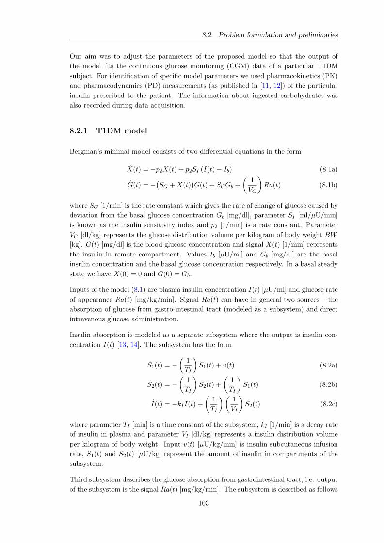
8.2. Problem formulation and preliminaries
Our aim was to adjust the parameters of the proposed model so that the output of
the model fits the continuous glucose monitoring (CGM) data of a particular T1DM
subject. For identification of specific model parameters we used pharmacokinetics (PK)
and pharmacodynamics (PD) measurements (as published in [11, 12]) of the particular
insulin prescribed to the patient. The information about ingested carbohydrates was
also recorded during data acquisition.
8.2.1 T1DM model
Bergman’s minimal model consists of two differential equations in the form
X(t) = −p2X(t) + p2SI (I(t)− Ib) (8.1a)
G(t) = −(SG +X(t)
)G(t) + SGGb +
(1
VG
)Ra(t) (8.1b)
where SG [1/min] is the rate constant which gives the rate of change of glucose caused by
deviation from the basal glucose concentration Gb [mg/dl], parameter SI [ml/µU/min]
is known as the insulin sensitivity index and p2 [1/min] is a rate constant. Parameter
VG [dl/kg] represents the glucose distribution volume per kilogram of body weight BW
[kg]. G(t) [mg/dl] is the blood glucose concentration and signal X(t) [1/min] represents
the insulin in remote compartment. Values Ib [µU/ml] and Gb [mg/dl] are the basal
insulin concentration and the basal glucose concentration respectively. In a basal steady
state we have X(0) = 0 and G(0) = Gb.
Inputs of the model (8.1) are plasma insulin concentration I(t) [µU/ml] and glucose rate
of appearance Ra(t) [mg/kg/min]. Signal Ra(t) can have in general two sources – the
absorption of glucose from gastro-intestinal tract (modeled as a subsystem) and direct
intravenous glucose administration.
Insulin absorption is modeled as a separate subsystem where the output is insulin con-
centration I(t) [13, 14]. The subsystem has the form
S1(t) = −(
1
TI
)S1(t) + v(t) (8.2a)
S2(t) = −(
1
TI
)S2(t) +
(1
TI
)S1(t) (8.2b)
I(t) = −kII(t) +
(1
TI
)(1
VI
)S2(t) (8.2c)
where parameter TI [min] is a time constant of the subsystem, kI [1/min] is a decay rate
of insulin in plasma and parameter VI [dl/kg] represents a insulin distribution volume
per kilogram of body weight. Input v(t) [µU/kg/min] is insulin subcutaneous infusion
rate, S1(t) and S2(t) [µU/kg] represent the amount of insulin in compartments of the
subsystem.
Third subsystem describes the glucose absorption from gastrointestinal tract, i.e. output
of the subsystem is the signal Ra(t) [mg/kg/min]. The subsystem is described as follows
103
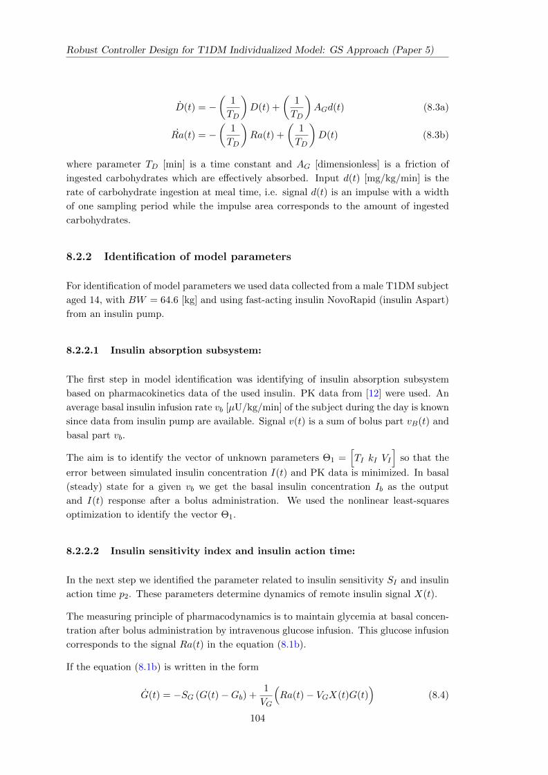
Robust Controller Design for T1DM Individualized Model: GS Approach (Paper 5)
D(t) = −(
1
TD
)D(t) +
(1
TD
)AGd(t) (8.3a)
Ra(t) = −(
1
TD
)Ra(t) +
(1
TD
)D(t) (8.3b)
where parameter TD [min] is a time constant and AG [dimensionless] is a friction of
ingested carbohydrates which are effectively absorbed. Input d(t) [mg/kg/min] is the
rate of carbohydrate ingestion at meal time, i.e. signal d(t) is an impulse with a width
of one sampling period while the impulse area corresponds to the amount of ingested
carbohydrates.
8.2.2 Identification of model parameters
For identification of model parameters we used data collected from a male T1DM subject
aged 14, with BW = 64.6 [kg] and using fast-acting insulin NovoRapid (insulin Aspart)
from an insulin pump.
8.2.2.1 Insulin absorption subsystem:
The first step in model identification was identifying of insulin absorption subsystem
based on pharmacokinetics data of the used insulin. PK data from [12] were used. An
average basal insulin infusion rate vb [µU/kg/min] of the subject during the day is known
since data from insulin pump are available. Signal v(t) is a sum of bolus part vB(t) and
basal part vb.
The aim is to identify the vector of unknown parameters Θ1 =[TI kI VI
]so that the
error between simulated insulin concentration I(t) and PK data is minimized. In basal
(steady) state for a given vb we get the basal insulin concentration Ib as the output
and I(t) response after a bolus administration. We used the nonlinear least-squares
optimization to identify the vector Θ1.
8.2.2.2 Insulin sensitivity index and insulin action time:
In the next step we identified the parameter related to insulin sensitivity SI and insulin
action time p2. These parameters determine dynamics of remote insulin signal X(t).
The measuring principle of pharmacodynamics is to maintain glycemia at basal concen-
tration after bolus administration by intravenous glucose infusion. This glucose infusion
corresponds to the signal Ra(t) in the equation (8.1b).
If the equation (8.1b) is written in the form
G(t) = −SG (G(t)−Gb) +1
VG
(Ra(t)− VGX(t)G(t)
)(8.4)
104
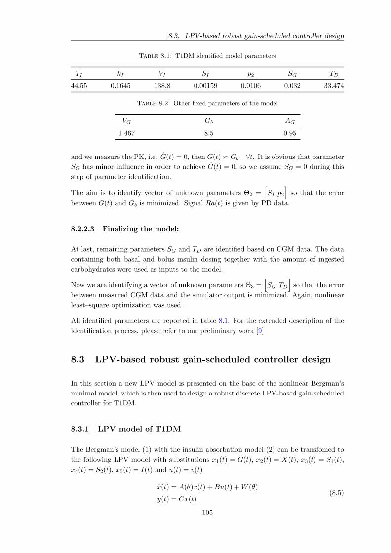
8.3. LPV-based robust gain-scheduled controller design
Table 8.1: T1DM identified model parameters
TI kI VI SI p2 SG TD
44.55 0.1645 138.8 0.00159 0.0106 0.032 33.474
Table 8.2: Other fixed parameters of the model
VG Gb AG
1.467 8.5 0.95
and we measure the PK, i.e. G(t) = 0, then G(t) ≈ Gb ∀t. It is obvious that parameter
SG has minor influence in order to achieve G(t) = 0, so we assume SG = 0 during this
step of parameter identification.
The aim is to identify vector of unknown parameters Θ2 =[SI p2
]so that the error
between G(t) and Gb is minimized. Signal Ra(t) is given by PD data.
8.2.2.3 Finalizing the model:
At last, remaining parameters SG and TD are identified based on CGM data. The data
containing both basal and bolus insulin dosing together with the amount of ingested
carbohydrates were used as inputs to the model.
Now we are identifying a vector of unknown parameters Θ3 =[SG TD
]so that the error
between measured CGM data and the simulator output is minimized. Again, nonlinear
least–square optimization was used.
All identified parameters are reported in table 8.1. For the extended description of the
identification process, please refer to our preliminary work [9]
8.3 LPV-based robust gain-scheduled controller design
In this section a new LPV model is presented on the base of the nonlinear Bergman’s
minimal model, which is then used to design a robust discrete LPV-based gain-scheduled
controller for T1DM.
8.3.1 LPV model of T1DM
The Bergman’s model (1) with the insulin absorbation model (2) can be transfomed to
the following LPV model with substitutions x1(t) = G(t), x2(t) = X(t), x3(t) = S1(t),
x4(t) = S2(t), x5(t) = I(t) and u(t) = v(t)
x(t) = A(θ)x(t) +Bu(t) +W (θ)
y(t) = Cx(t)(8.5)
105
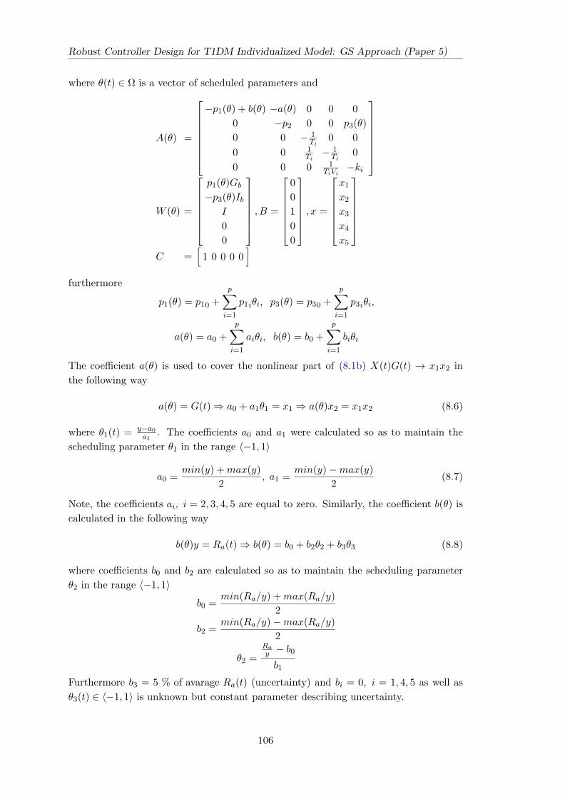
Robust Controller Design for T1DM Individualized Model: GS Approach (Paper 5)
where θ(t) ∈ Ω is a vector of scheduled parameters and
A(θ) =
−p1(θ) + b(θ) −a(θ) 0 0 0
0 −p2 0 0 p3(θ)
0 0 − 1Ti
0 0
0 0 1Ti− 1Ti
0
0 0 0 1TiVi
−ki
W (θ) =
p1(θ)Gb−p3(θ)Ib
I
0
0
, B =
0
0
1
0
0
, x =
x1
x2
x3
x4
x5
C =
[1 0 0 0 0
]furthermore
p1(θ) = p10 +
p∑i=1
p1iθi, p3(θ) = p30 +
p∑i=1
p3iθi,
a(θ) = a0 +
p∑i=1
aiθi, b(θ) = b0 +
p∑i=1
biθi
The coefficient a(θ) is used to cover the nonlinear part of (8.1b) X(t)G(t) → x1x2 in
the following way
a(θ) = G(t)⇒ a0 + a1θ1 = x1 ⇒ a(θ)x2 = x1x2 (8.6)
where θ1(t) = y−a0a1
. The coefficients a0 and a1 were calculated so as to maintain the
scheduling parameter θ1 in the range 〈−1, 1〉
a0 =min(y) +max(y)
2, a1 =
min(y)−max(y)
2(8.7)
Note, the coefficients ai, i = 2, 3, 4, 5 are equal to zero. Similarly, the coefficient b(θ) is
calculated in the following way
b(θ)y = Ra(t)⇒ b(θ) = b0 + b2θ2 + b3θ3 (8.8)
where coefficients b0 and b2 are calculated so as to maintain the scheduling parameter
θ2 in the range 〈−1, 1〉b0 =
min(Ra/y) +max(Ra/y)
2
b2 =min(Ra/y)−max(Ra/y)
2
θ2 =
Ray − b0b1
Furthermore b3 = 5 % of avarage Ra(t) (uncertainty) and bi = 0, i = 1, 4, 5 as well as
θ3(t) ∈ 〈−1, 1〉 is unknown but constant parameter describing uncertainty.
106
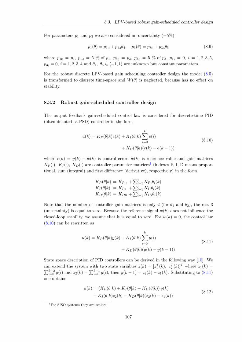
8.3. LPV-based robust gain-scheduled controller design
For parameters p1 and p3 we also considered an uncertainty (±5%)
p1(θ) = p10 + p14θ4, p3(θ) = p30 + p35θ5 (8.9)
where p10 = p1, p14 = 5 % of p1, p30 = p3, p35 = 5 % of p3, p1i = 0, i = 1, 2, 3, 5,
p3i = 0, i = 1, 2, 3, 4 and θ4, θ5 ∈ 〈−1, 1〉 are unknown but constant parameters.
For the robust discrete LPV-based gain scheduling controller design the model (8.5)
is transformed to discrete time-space and W (θ) is neglected, because has no effect on
stability.
8.3.2 Robust gain-scheduled controller design
The output feedback gain-scheduled control law is considered for discrete-time PID
(often denoted as PSD) controller in the form
u(k) = KP (θ|k)e(k) +KI(θ|k)
k∑i=0
e(i)
+KD(θ|k)(e(k)− e(k − 1))
(8.10)
where e(k) = y(k) − w(k) is control error, w(k) is reference value and gain matrices
KP (·), KI(·), KD(·) are controller parameter matrices1 (indexes P, I, D means propor-
tional, sum (integral) and first difference (derivative), respectively) in the form
KP (θ|k) = KP 0 +∑p
i=1KP iθi(k)
KI(θ|k) = KI0 +∑p
i=1KI iθi(k)
KD(θ|k) = KD0 +∑p
i=1KDiθi(k)
Note that the number of controller gain matrices is only 2 (for θ1 and θ2), the rest 3
(uncertainty) is equal to zero. Because the reference signal w(k) does not influence the
closed-loop stability, we assume that it is equal to zero. For w(k) = 0, the control law
(8.10) can be rewritten as
u(k) = KP (θ|k)y(k) +KI(θ|k)k∑i=0
y(i)
+KD(θ|k)(y(k)− y(k − 1))
(8.11)
State space description of PID controllers can be derived in the following way [15]. We
can extend the system with two state variables z(k) = [zT1 (k), zT2 (k)]T where z1(k) =∑k−2i=0 y(i) and z2(k) =
∑k−1i=0 y(i), then y(k − 1) = z2(k)− z1(k). Substituting to (8.11)
one obtains
u(k) = (KP (θ|k) +KI(θ|k) +KD(θ|k)) y(k)
+KI(θ|k)z2(k)−KD(θ|k)(z2(k)− z1(k))(8.12)
1For SISO systems they are scalars.
107
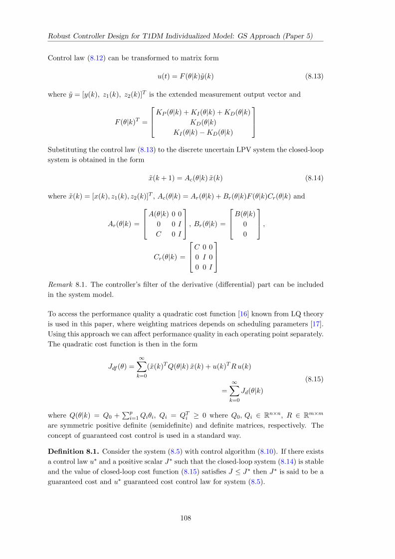
Robust Controller Design for T1DM Individualized Model: GS Approach (Paper 5)
Control law (8.12) can be transformed to matrix form
u(t) = F (θ|k)y(k) (8.13)
where y = [y(k), z1(k), z2(k)]T is the extended measurement output vector and
F (θ|k)T =
KP (θ|k) +KI(θ|k) +KD(θ|k)
KD(θ|k)
KI(θ|k)−KD(θ|k)
Substituting the control law (8.13) to the discrete uncertain LPV system the closed-loop
system is obtained in the form
x(k + 1) = Ac(θ|k) x(k) (8.14)
where x(k) = [x(k), z1(k), z2(k)]T , Ac(θ|k) = Ar(θ|k) +Br(θ|k)F (θ|k)Cr(θ|k) and
Ar(θ|k) =
A(θ|k) 0 0
0 0 I
C 0 I
, Br(θ|k) =
B(θ|k)
0
0
,Cr(θ|k) =
C 0 0
0 I 0
0 0 I
Remark 8.1. The controller’s filter of the derivative (differential) part can be included
in the system model.
To access the performance quality a quadratic cost function [16] known from LQ theory
is used in this paper, where weighting matrices depends on scheduling parameters [17].
Using this approach we can affect performance quality in each operating point separately.
The quadratic cost function is then in the form
Jdf (θ) =∞∑k=0
(x(k)TQ(θ|k) x(k) + u(k)TRu(k)
=
∞∑k=0
Jd(θ|k)
(8.15)
where Q(θ|k) = Q0 +∑p
i=1Qiθi, Qi = QTi ≥ 0 where Q0, Qi ∈ Rn×n, R ∈ Rm×m
are symmetric positive definite (semidefinite) and definite matrices, respectively. The
concept of guaranteed cost control is used in a standard way.
Definition 8.1. Consider the system (8.5) with control algorithm (8.10). If there exists
a control law u∗ and a positive scalar J∗ such that the closed-loop system (8.14) is stable
and the value of closed-loop cost function (8.15) satisfies J ≤ J∗ then J∗ is said to be a
guaranteed cost and u∗ guaranteed cost control law for system (8.5).
108
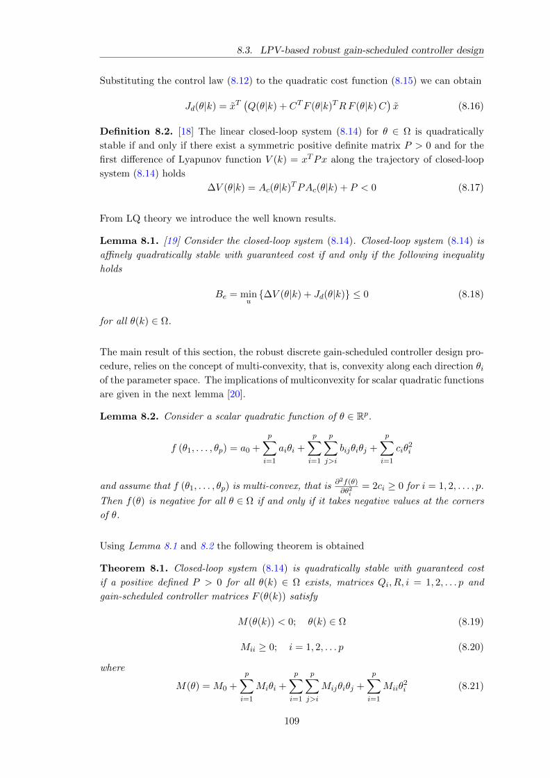
8.3. LPV-based robust gain-scheduled controller design
Substituting the control law (8.12) to the quadratic cost function (8.15) we can obtain
Jd(θ|k) = xT(Q(θ|k) + CTF (θ|k)TRF (θ|k)C
)x (8.16)
Definition 8.2. [18] The linear closed-loop system (8.14) for θ ∈ Ω is quadratically
stable if and only if there exist a symmetric positive definite matrix P > 0 and for the
first difference of Lyapunov function V (k) = xTPx along the trajectory of closed-loop
system (8.14) holds
∆V (θ|k) = Ac(θ|k)TPAc(θ|k) + P < 0 (8.17)
From LQ theory we introduce the well known results.
Lemma 8.1. [19] Consider the closed-loop system (8.14). Closed-loop system (8.14) is
affinely quadratically stable with guaranteed cost if and only if the following inequality
holds
Be = minu∆V (θ|k) + Jd(θ|k) ≤ 0 (8.18)
for all θ(k) ∈ Ω.
The main result of this section, the robust discrete gain-scheduled controller design pro-
cedure, relies on the concept of multi-convexity, that is, convexity along each direction θiof the parameter space. The implications of multiconvexity for scalar quadratic functions
are given in the next lemma [20].
Lemma 8.2. Consider a scalar quadratic function of θ ∈ Rp.
f (θ1, . . . , θp) = a0 +
p∑i=1
aiθi +
p∑i=1
p∑j>i
bijθiθj +
p∑i=1
ciθ2i
and assume that f (θ1, . . . , θp) is multi-convex, that is ∂2f(θ)∂θ2i
= 2ci ≥ 0 for i = 1, 2, . . . , p.
Then f(θ) is negative for all θ ∈ Ω if and only if it takes negative values at the corners
of θ.
Using Lemma 8.1 and 8.2 the following theorem is obtained
Theorem 8.1. Closed-loop system (8.14) is quadratically stable with guaranteed cost
if a positive defined P > 0 for all θ(k) ∈ Ω exists, matrices Qi, R, i = 1, 2, . . . p and
gain-scheduled controller matrices F (θ(k)) satisfy
M(θ(k)) < 0; θ(k) ∈ Ω (8.19)
Mii ≥ 0; i = 1, 2, . . . p (8.20)
where
M(θ) = M0 +
p∑i=1
Miθi +
p∑i=1
p∑j>i
Mijθiθj +
p∑i=1
Miiθ2i (8.21)
109
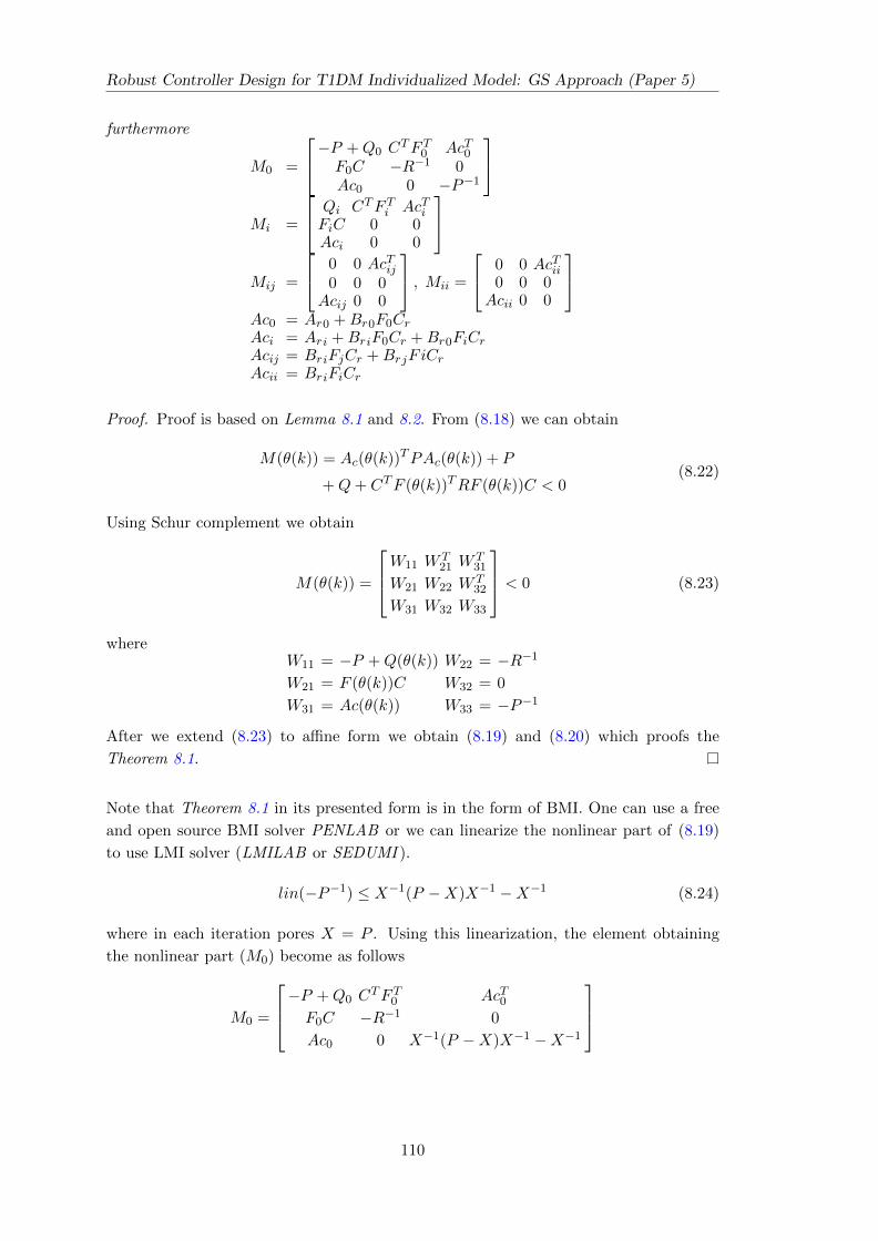
Robust Controller Design for T1DM Individualized Model: GS Approach (Paper 5)
furthermore
M0 =
−P +Q0 CTF T0 AcT0
F0C −R−1 0Ac0 0 −P−1
Mi =
Qi CTF Ti AcTiFiC 0 0Aci 0 0
Mij =
0 0 AcTij0 0 0
Acij 0 0
, Mii =
0 0 AcTii0 0 0Acii 0 0
Ac0 = Ar0 +Br0F0CrAci = Ari +BriF0Cr +Br0FiCrAcij = BriFjCr +BrjFiCrAcii = BriFiCr
Proof. Proof is based on Lemma 8.1 and 8.2. From (8.18) we can obtain
M(θ(k)) = Ac(θ(k))TPAc(θ(k)) + P
+Q+ CTF (θ(k))TRF (θ(k))C < 0(8.22)
Using Schur complement we obtain
M(θ(k)) =
W11 WT21 W
T31
W21 W22 WT32
W31 W32 W33
< 0 (8.23)
whereW11 = −P +Q(θ(k)) W22 = −R−1
W21 = F (θ(k))C W32 = 0
W31 = Ac(θ(k)) W33 = −P−1
After we extend (8.23) to affine form we obtain (8.19) and (8.20) which proofs the
Theorem 8.1.
Note that Theorem 8.1 in its presented form is in the form of BMI. One can use a free
and open source BMI solver PENLAB or we can linearize the nonlinear part of (8.19)
to use LMI solver (LMILAB or SEDUMI ).
lin(−P−1) ≤ X−1(P −X)X−1 −X−1 (8.24)
where in each iteration pores X = P . Using this linearization, the element obtaining
the nonlinear part (M0) become as follows
M0 =
−P +Q0 CTF T0 AcT0
F0C −R−1 0
Ac0 0 X−1(P −X)X−1 −X−1
110
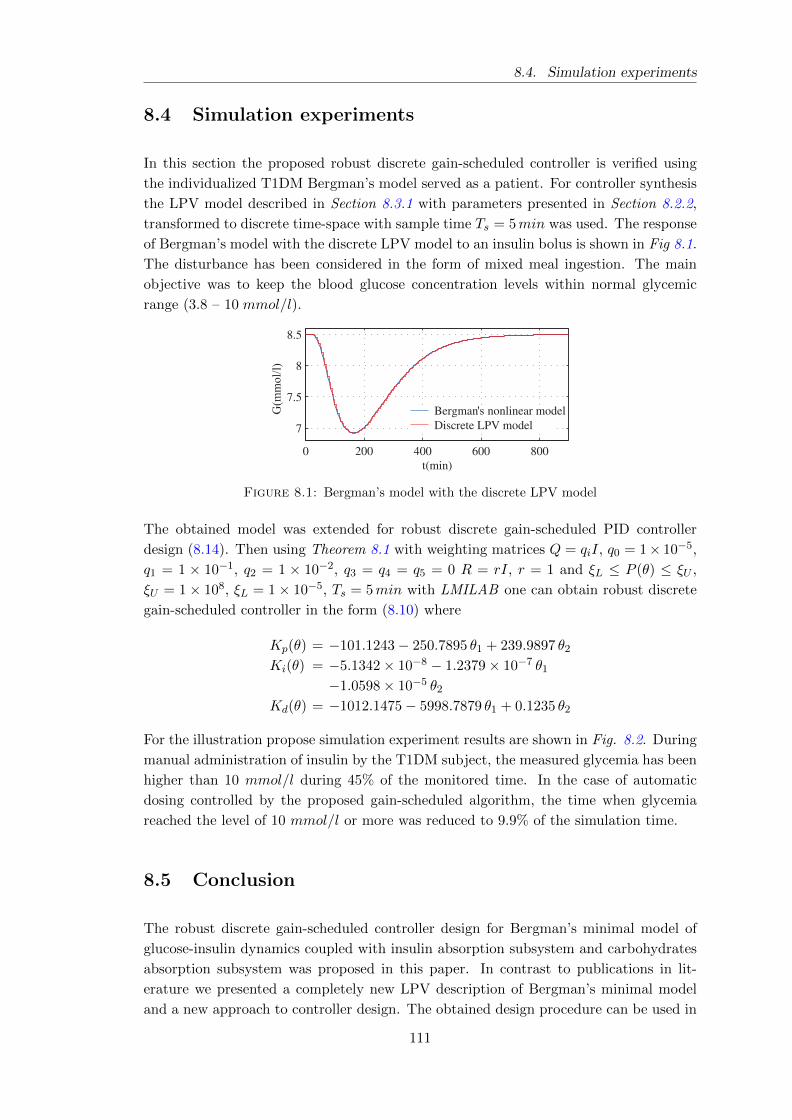
8.4. Simulation experiments
8.4 Simulation experiments
In this section the proposed robust discrete gain-scheduled controller is verified using
the individualized T1DM Bergman’s model served as a patient. For controller synthesis
the LPV model described in Section 8.3.1 with parameters presented in Section 8.2.2,
transformed to discrete time-space with sample time Ts = 5min was used. The response
of Bergman’s model with the discrete LPV model to an insulin bolus is shown in Fig 8.1.
The disturbance has been considered in the form of mixed meal ingestion. The main
objective was to keep the blood glucose concentration levels within normal glycemic
range (3.8 – 10 mmol/l).
Figure 8.1: Bergman’s model with the discrete LPV model
The obtained model was extended for robust discrete gain-scheduled PID controller
design (8.14). Then using Theorem 8.1 with weighting matrices Q = qiI, q0 = 1× 10⁻⁵,
q1 = 1 × 10⁻¹, q2 = 1 × 10⁻², q3 = q4 = q5 = 0 R = rI, r = 1 and ξL ≤ P (θ) ≤ ξU ,
ξU = 1× 10⁸, ξL = 1× 10⁻⁵, Ts = 5min with LMILAB one can obtain robust discrete
gain-scheduled controller in the form (8.10) where
Kp(θ) = −101.1243− 250.7895 θ1 + 239.9897 θ2
Ki(θ) = −5.1342× 10⁻⁸ − 1.2379× 10⁻⁷ θ1
−1.0598× 10⁻⁵ θ2
Kd(θ) = −1012.1475− 5998.7879 θ1 + 0.1235 θ2
For the illustration propose simulation experiment results are shown in Fig. 8.2. During
manual administration of insulin by the T1DM subject, the measured glycemia has been
higher than 10 mmol/l during 45% of the monitored time. In the case of automatic
dosing controlled by the proposed gain-scheduled algorithm, the time when glycemia
reached the level of 10 mmol/l or more was reduced to 9.9% of the simulation time.
8.5 Conclusion
The robust discrete gain-scheduled controller design for Bergman’s minimal model of
glucose-insulin dynamics coupled with insulin absorption subsystem and carbohydrates
absorption subsystem was proposed in this paper. In contrast to publications in lit-
erature we presented a completely new LPV description of Bergman’s minimal model
and a new approach to controller design. The obtained design procedure can be used in
111
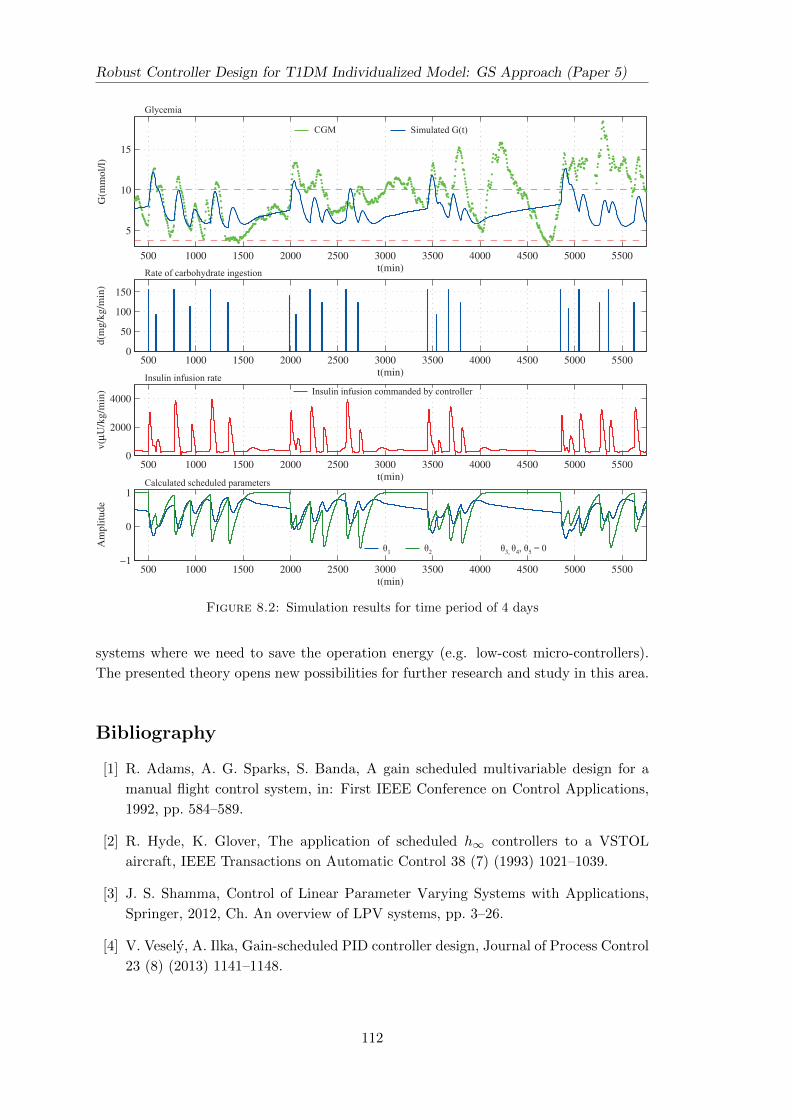
Robust Controller Design for T1DM Individualized Model: GS Approach (Paper 5)
Figure 8.2: Simulation results for time period of 4 days
systems where we need to save the operation energy (e.g. low-cost micro-controllers).
The presented theory opens new possibilities for further research and study in this area.
Bibliography
[1] R. Adams, A. G. Sparks, S. Banda, A gain scheduled multivariable design for a
manual flight control system, in: First IEEE Conference on Control Applications,
1992, pp. 584–589.
[2] R. Hyde, K. Glover, The application of scheduled h∞ controllers to a VSTOL
aircraft, IEEE Transactions on Automatic Control 38 (7) (1993) 1021–1039.
[3] J. S. Shamma, Control of Linear Parameter Varying Systems with Applications,
Springer, 2012, Ch. An overview of LPV systems, pp. 3–26.
[4] V. Vesely, A. Ilka, Gain-scheduled PID controller design, Journal of Process Control
23 (8) (2013) 1141–1148.
112
Bibliography
[5] A. Ilka, V. Vesely, Discrete gain-scheduled controller design: Variable weighting
approach, in: 15th International Carpathian Control Conference (ICCC), 2014,
2014, pp. 186–191.
[6] V. Vesely, A. Ilka, PID robust gain-scheduled controller design, in: 2014 European
Control Conference (ECC), 2014, pp. 2756–2761.
[7] M. Tarnık, J. Murgas, E. Miklovicova, v. Farkas, Adaptive Control of Time-delayed
Systems with Application for Control of Glucose Concentration in Type 1 Diabetic
Patients, in: 11th IFAC International Workshop on Adaptation and Learning in
Control and Signal Processing - July 3-5 2013, Caen, France, 2013.
[8] M. Tarnık, E. Miklovicova, J. Murgas, I. Ottinger, T. Ludwig, Model Reference
Adaptive Control of Glucose in Type 1 Diabetics: A Simulation Study, in: Proceed-
ings of the 19th IFAC World Congress, 2014, Cape Town International Convention
Centre, Cape Town, South Africa., 2014.
[9] I. Ottinger, T. Ludwig, E. Miklovicova, V. Batora, J. Murgas, M. Tarnık, Individu-
alized T1DM Simulator for Verification of Adaptive Controller, process Control 2015
(submitted) (January 2015).
[10] R. Bergman, Y. Ider, C. Bowden, C. Cobelli, Quantitative estimation of insulin
sensitivity, Am. J. Physiol. Endocrinol. Metab 236 (6) (1979) E667–E677.
[11] Novo-Nordisk, NovoRapid (insulin aspart) - Product Monograph, Watermeadow
Medical, Two Rivers House, Station Lane, Witney, Oxfordshire OX28 4BH, UK on
behalf of Novo Nordisk A/S, 2002.
[12] S. Mudaliar, F. A. Lindberg, M. Joyce, P. Beerdsen, P. Strange, A. Lin, R. R.
Henry, Insulin Aspart (B28 Asp-Insulin): A Fast-Acting Analog of Human Insulin,
Diabetes Care 22 (9) (1999) 1501–1506.
[13] P. Herrero, P. Georgiou, N. Oliver, M. Reddy, D. Johnston, C. Toumazou, A Com-
posite Model of Glucagon-Glucose Dynamics for In Silico Testing of Bihormonal
Glucose Controllers, Journal of Diabetes Science and Technology 7 (4) (2013) 941–
951.
[14] R. Hovorka, V. Canonico, L. J. Chassin, U. Haueter, M. Massi-Benedetti, M. O.
Federici, T. R. Pieber, H. C. Schaller, L. Schaupp, T. Vering, M. E. Wilinska,
Nonlinear model predictive control of glucose concentration in subjects with type
1 diabetes, Physiological Measurement 25 (4) (2004) 905.
[15] V. Vesely, D. Rosinova, Robust PID-PSD Controller Design: BMI Approach, Asian
Journal of Control 15 (2) (2013) 469–478.
[16] J. Engwerda, A. Weeren, A result on output feedback linear quadratic control,
Automatica 44 (1) (2008) 265–271.
[17] A. Ilka, V. Vesely, Gain-Scheduled Controller Design: Variable Weighting Ap-
proach, Journal of Electrical Engineering 65 (2) (2014) 116–120.
113
Robust Controller Design for T1DM Individualized Model: GS Approach (Paper 5)
[18] P. Apkarian, P. Gahinet, G. Becker, Self-Scheduled H∞ Control of Linear
Parameter-Varying Systems: A Design Example, Automatica 31 (9) (1995) 1251–
1261.
[19] V. Kuncevic, M. Lycak, Control system design using Lyapunov function approach
(in Russian), Nauka, Moskva, 1977.
[20] P. Gahinet, P. Apkarian, M. Chilali, Affine parameter-dependent Lyapunov func-
tions and real parametric uncertainty, IEEE Transactions on Automatic Control
41 (3) (1996) 436–442.
114
9
Novel approach to switched controller
design for linear continuous-time
systems (Paper 6)
Abstract
In this paper we study the novel approach to the design of an output feedback switched
controller with an arbitrary switching algorithm for continuous-time invariant systems
which is described by a novel plant model as a gain-scheduled plant using the multiple
quadratic stability and quadratic stability approaches. In the proposed design proced-
ure there is no need to use the notion of the ”dwell-time”. The obtained results are
in the form of bilinear matrix inequalities (BMI). Numerical examples show that in the
proposed method the design procedure is less conservative and gives more possibilities
than that described in the papers published previously.
Keywords: Switched system, continuous time system, output feedback, quadratic sta-
bility, multi quadratic stability.
9.1 Introduction
Switched systems have played an important role in the past decade. Motivation for
studying switched systems comes from two facts:
• switched systems have numerous applications in the control of real plants, and
• in real control, there are dynamical systems that cannot be stabilized by any
continuous static output/state feedback control law, but a stabilizing switching
control scheme can be found.
115
Novel approach to switched controller design for linear systems (Paper 6)
Switched systems constitute an important class. The switched system consists of a con-
tinuous or discrete time system and a switching law that specifies the switching between
them. It is pointed out in [1–4] that the stability of switched systems plays an important
role in the analysis and design of switched controllers. There are at least two approaches
to the stability analysis of switched systems: The quadratic stability approach with a
common Lyapunov function gives the stability under an arbitrary switching law, and
Multiple Lyapunov functions, which is less conservative. A huge number of references
can be found on the switched control of linear discrete-time invariant systems, but in the
field of linear continuous-time invariant systems the number of references is rather small.
Representatives are the following references [5–9]. In the first paper the authors intro-
duce, into the switched controller design procedure, the notion of dwell-time Td (minimal
time interval between switching). In the stability analysis condition of switched systems
the dwell-time is in the term eAcTd (Ac-closed-loop matrix (9.4)). The proposed design
procedure for stability analysis and switching controller design for the real switching
time interval T ≥ Td becomes rather conservative. The above ”dwell-time term” com-
plicated the switched controller design procedure for continuous-time systems. In [6]
sufficient conditions are given for the stability of linear systems with a dwell-time and
with polytopic type parameter uncertainty. A Lyapunov function, in quadratic form for
each mode, which is non-increasing at the switching instants is assigned to each mode.
During the dwell-time this function varies piecewise linearly in time after switching oc-
curs. The proposed method was applied to stabilization via the state feedback for both
nominal and uncertain cases. Since within the dwell-time the Lyapunov function varies
piecewise linearly and the real switching time interval T > Td, the switching controller
design procedure becomes rather conservative. In [7] the stability analysis problem for
a class of switched positive linear systems with average dwell time switching is invest-
igated. Paper [8] investigates the stability of a class of switched linear systems and
proposes a number of new results on the stability analysis. A novel analysis method is
developed by using the 2-norm technique, and then several stability results are obtained
based on the new analysis method. It is shown that the main results obtained in this
paper not only guarantee the stability of the systems under arbitrary switching but also
provide an algorithm to find the minimum dwell time with which switches make the
switched systems stable. Dwell-time switching is a logic for orchestrating the switch-
ing between controllers in order to control a proces with a highly uncertain model [9].
The idea of dwell-time switching is to use a parameter tuner which switches controller
parameter values rather than continuously adjusting them. Such switched system con-
sisting of two interconnected subsystems, namely a ”continuous part” and a ”dwell-time
switching logic”. Together these two subsystems constitute a parameter tuner which
is a bona fide hybrid (switched) system. Above system generated ”switching logic” to
make estimation error (performance) ”small” in some sense [9]. Note that implementa-
tion of dwell-time switching logic requires capable of minimizing some performance over
the set of controller in real time. In this paper the proposed switched controller design
procedure for continuous-time systems has none of the above mentioned drawbacks due
to dwell-time consideration. An overview of switched systems can be found in [1, 3, 10].
In this paper, new quadratic stability and multi quadratic stability conditions of closed-
loop switched systems for arbitrarily switching [3] are given using a new model of
116
9.2. Preliminaries and problem formulation
switched continuous time linear systems. In the proposed approach to switching con-
troller design for continuous time systems there is no need to use the approach of the
”dwell-time” [5, 6]. The proposed switched controller design procedure can easily be
expanded to the case of robust switched controller design [11] with multi parameter
dependent quadratic stability.
Organization of the paper is as follows. Section 9.2 includes problem formulation of the
switched controller design using the novel proposed model and some preliminary results
are given. In Section 9.3 sufficient stability conditions in the form of BMI for the case
of quadratic and multi quadratic approach are given and in Section 9.4 the obtained
results are illustrated on some examples.
Hereafter, the following notational conditions will be adopted. Given a symmetric mat-
rix P = P T ∈ Rn×n, the inequality P > 0 denotes matrix positive definiteness. Symbol
∗ denotes a block that is transposed and complex conjugated to the respective symmet-
rically placed one. I denotes the identity matrix of corresponding dimensions.
9.2 Preliminaries and problem formulation
Let us consider a class of linear continuous-time invariant switched systems∑σ : x(t) = A(θ)x(t) +B(θ)u(t)
y(t) = Cx(t)
x(0) = x0
(9.1)
where x(t) ∈ Rn is the state vector, u(t) ∈ Rm is the control vector, y(t) ∈ Rl is the
output vector of the system to be controlled, and σ ∈ S = 1, 2, . . . , p is an arbitrarily
switching algorithm. The arbitrary switching algorithm σ is a piecewise constant, right
continuous function which specifies at each time the index of the active closed-loop
system [3, 12], p is the number of switched modes of linear systems and
A(θ) = A0 +
p∑i=1
Aiθi , B(θ) = B0 +
p∑i=1
Biθi (9.2)
where∑p
i=1 θi = 1, θi ∈ 〈0, 1〉 ∈ Ωθ, i = 1, 2, . . . , p are switching parameters. For
calculation of all the above matrices in (9.1) see the example. Note that for switching
systems the stable steady state points of switching parameters θi, i = 1, 2, . . . , p are
equal to 0 or 1. If the switching parameter θi, i = 1, 2, . . . , p differs from 0 or 1, it is
moving to one of the stable points with the rate of θi change θi, i = 1, 2, . . . , p. There
are two possibilities for switching parameters:
• the rates of change of switching parameters are infinite, that is θi = 1 holds for
the i-th mode and θj = 0 for j = 1, 2, . . . , p, j 6= i (quadratic stability approach),
or
117
Novel approach to switched controller design for linear systems (Paper 6)
• the rates of change of switching parameters are finite, assume that the system
switched from i to j mode. For this case one has θi + θj = 1, θi + θj = 0 and
θk = 0, k 6= i, j (multiple quadratic stability approach).
For both cases θi, i = 1, 2, . . . , p are known and the number of system mode or the
number of vertices is equal to ”p”. Note that number of vertices for polytopic system is
2p.
The switched output feedback control law is considered in the form
u(t) = F (θ)y(t) = F (θ)Cx(t) (9.3)
where
F (θ) = F0 +
p∑i=1
Fiθi
The structure of matrices Fi, i = 0, 1, . . . , p can be prescribed, for decentralized control
structure Fi is a block diagonal matrix and so on. The closed-loop system is obtained
from Eqs. (9.1) and (9.3)
x(t) = (A(θ) +B(θ)F (θ)C)x(t) = Ac(θ)x(t) (9.4)
To access the system performance, we consider a standard positive definite quadratic
cost function with respect to state x and control u.
J =
∫ ∞0
(x(t)T (t)Qx(t) + uT (t)Ru(t)
)dt =
∫ ∞0
J(t)dt (9.5)
Let us recall some results on the optimal control of time varying systems.
Lemma 9.1. [13] Let there exists a scalar positive definite function V (x, t) such that
limt→∞
V (x, t) = 0 which satisfies
minu(t)∈Ωu
∂V
∂xAc(θ) +
∂V
∂t+ J(t)
= 0 (9.6)
The control algorithm u(t) = u∗(x, t) ∈ Ωu obtained from (9.6) ensures closed-loop
stability and the optimal value of the cost function (9.5) as J∗ = J(x0, t0) = V (x(0), t0).
Equation (9.6) is known as the Bellman-Lyapunov equation and function V (x, t) which
satisfies (9.6) is the Lyapunov function. For a particular structure of the Lyapunov
function the optimal control algorithm reduces from ”if and only if” to ”if”, and for
switched systems, robust control and so on to a guaranteed cost.
Definition 9.1. Consider system (9.1) and controller (9.3). If there exist a control
law u∗(x, t) and a positive scalar J∗ such that the respective closed-loop system (9.4) is
stable and the value of the closed-loop cost function (9.5) satisfies J ≤ J∗, then J∗ is
said to be the guaranteed cost and u∗(x, t) is said to be the guaranteed cost control law
for system (9.4).
118
9.3. Switched controller design
Definition 9.2. [4] The switched linear closed-loop system (9.4) is said to be quadrat-
ically stabilizable via output feedback if there exists a Lyapunov function of the form
V = x(t)TPx(t), P > 0, a positive number ε > 0 and a arbitrary switching rule σ such
thatdV
dt≤ −εx(t)Tx(t) (9.7)
Definition 9.3. The switched linear closed-loop system (9.4) is said to be multiple
quadratically stabilizable via output feedback if there exists a Lyapunov function of the
form V (θ) = x(t)TP (θ)x(t), P (θ) > 0, a positive number ε > 0 and a arbitrary switching
rule σ such thatdV (θ)
dt≤ −εx(t)Tx(t) (9.8)
Lemma 9.2. [14], [3] Consider a closed-loop system (9.4) with control algorithm (9.3).
Control algorithm (9.3) will be a cost guaranteed algorithm if there exists a positive
scalar ε such that for the time derivative of the positive definite Lyapunov function the
following condition holds
Be = minu(t)∈Ωu
∂V
∂xAc(θ) +
∂V
∂t+ J(t)
≤ −εx(t)Tx(t) (9.9)
when ε→ 0.
The following lemma plays an important role in the next development [15]
Lemma 9.3. Consider a scalar quadratic function of θi
f(θ) = a0 +
p∑i=1
aiθi +
p∑i=1
p∑j=i
bijθiθj (9.10)
and assume that f(θ) is multiconvex, that is
∂2f(θ)
∂θ2i
≥ 0, i = 1, 2, . . . , p (9.11)
then f(θ) is negative in the hyper rectangle θi ∈ 〈0, 1〉, i = 1, 2, . . . , p, if and only if it
takes negative values at the corners, that is if and only if f(θ) < 0 for θi = 0 or θi = 1,
i = 1, 2, . . . , p.
9.3 Switched controller design
In this paragraph two methods of switched controller design for linear continuous-time
invariant systems are presented. The first method is connected with the notion of
quadratic stability with respect to θ. We will assume that the rate of θ change is
infinite. Most of the literature on switched controller design concentrates on the case,
where switching can occur immediately, thus the rate of change of the switching signal
is infinite (ideal switching). In some real cases the rate of change of the switching signal
119
Novel approach to switched controller design for linear systems (Paper 6)
is finite (non ideal switching). This assumption will be used in the second approach
to obtain the switched controller design procedure. In the references on the design of
switched controllers for continuous-time systems there are no solution for the case of a
finite rate of change of switching signal. In this paper we for the first time set up the
case of the finite rate of change of the switching signal using the multi quadratic stability
approach to the closed loop switched systems. In the proposed approach to the switching
controller design for continuous time systems there is no need to use the approach of the
”dwell-time” [5, 6], which very complicated the switched controller design procedure.
9.3.1 Quadratic stability approach
The quadratic stability approach to the design of the switched controller for continuous
and discrete-time systems is well established. Because of the new model for continuous
time systems (9.1) in this part of the paper the proposed method is connected with the
notion of quadratic stability with respect to θ. We will assume that the rate of θ change
is infinite (ideal switching). From (9.9) the following lemma is obtained.
Lemma 9.4. Closed-loop Ac(θ) is quadratically stable with guaranteed cost if there exists
a positive definite Lyapunov matrix P such that the following inequality holds
ATc (θ)P + PAc(θ) +Q+ CTF (θ)TRF (θ)C ≤ 0 (9.12)
Substituting Ac(θ) (9.4) to (9.12) and using Lemmas 9.2 and 9.3 the following quadratic
stability conditions are obtained.
Theorem 9.1. Closed-loop system (9.4) is quadratically stable with guaranteed cost if
there exists a Lyapunov matrix P > 0 and matrices Q ≥ 0, R > 0 such that for an
arbitrarily switching rule σ the following matrix inequalities hold
a.)
(A0 +B0F0C)TP + P (A0 +B0F0C)
+Q+ CTF T0 RF0C = M0 ≤ 0(9.13)
b.)
M0 +Mi +Mii ≤ 0, i = 1, 2, . . . , p (9.14)
where
Mi = (Ai +B0FiC +BiF0C)TP
+ P (Ai +B0FiC +BiF0C)
+ CTF Ti RF0C + CTF T0 RFiC
(9.15)
and
Mii = (BiFiC)TP + PBiFiC + CTF Ti RFiC (9.16)
120
9.3. Switched controller design
c.)
Mii ≥ 0, for i = 1, 2, . . . , p (9.17)
provided that θi = 0 or θi = 1
Proof
Proof is based on (9.9), Lemma 9.2 and Lemma 9.3 and goes the same line as proof of
Theorem 9.2.
Equation (9.14) implies that for stability analysis of the switched system we have ob-
tained linear matrix inequalities (LMI) but for the switched controller design we have
obtained bilinear matrix inequalities (BMI).
9.3.2 Multiple Lyapunov function approach
In this subsection we will assume that for some realistic cases the switching signal rate
of change is finite (non ideal switching). As we mentioned above in the references,
there is no solution for these cases. The obtained results for a finite rate of change of
switching signal open the new possibilities for the designer (practical realization) and
for the theory of the switched controller design procedure, i.e., the design of a switched
robust controller, design of a switched controller for some type of nonlinear systems and
so on. Specifically
• for switching parameters it holds∑p
i=1 θi = 1,
θi ∈ 〈0 1〉 ∈ Ωθ.
• the rate of switching parameter variation θi is well defined at all times and satisfies
known boundaries
θi ∈ Ωt =θi ∈
⟨θi, θi
⟩, i = 1, 2, . . . , p
(9.18)
p∑i=1
θi = 0.
Main results for the switched controller design using the multiple quadratic stability
approach are given in the next theorem.
Theorem 9.2. Closed-loop system (9.4) is multiple quadratically stable with guaranteed
cost if there exist p+ 1 symmetric matrices P0, P1, . . . , Pp such that P0 +∑p
i=1 Piθi > 0
is positive definite for all switching parameters θi ∈ Ωθ, θi ∈ Ωt switched controller
parameters F (θ) satisfying
W (θ) ≤ 0
Wii ≥ 0, i = 1, 2, . . . , p(9.19)
for an arbitrary switching rule σ.
121
Novel approach to switched controller design for linear systems (Paper 6)
where
W (θ) = W0 +
p∑i=1
Wiθi +
p∑i=1
p∑j=1
Wijθiθj
W0 =
[w110 w120
wT120 w220
];Wi =
[w11i w12i
wT12i w22i
]
Wij =
[w11ij w12ij
wT12ij w22ij
]w110 = N1 +NT
1 , w11i = w11ij = 0
w120 = P0 +N2 −NT1 Ac0, w12i = Pi +N2 −NT
1 Aci
w12ij = N2 −NT1 Acij
w220 =
p∑k=1
Pkθk −NT2 Ac0 −ATc0N2 +Q+ CTF T0 RF0C
w22i = −NT2 Aci −ATciN2 + CTF T0 RFiC + CTF Ti RF0C
w22ij = −NT2 Acij −ATcijN2 + CTF Ti RFjC + CTF Tj RFiC
Ac0 = A0 +B0F0C, Aci = Ai +B0FiC +BiF0C
Acij = BiFjC
Proof
For the first derivative of the Lyapunov function V (θ) = x(t)TP (θ)x(t) one obtains
dV (θ)
dt= x(t)TP (θ)x(t) + x(t)TP (θ)x(t) + x(t)TP (θ)x(t) =
[x(t)T x(t)T ]
[0 P (θ)
P (θ) P (θ)
][x(t)T x(t)T ]T
where
P (θ) =
p∑i=1
Piθi ≤p∑i=1
Piθi
assuming Pi > 0, i = 1, 2 . . . , p. For closed-loop system (9.4) one can write (x(t) = x)
[xTNT1 + xTNT
2 ][x−Ac(θ)x] + ([xTNT1 + xTNT
2 ][x−Ac(θ)x])T = 0 (9.20)
where N1, N2 ∈ Rn×n are auxiliary matrices. Summarizing the above two equations, for
the first derivative of the Lyapunov function it holds
dV (θ)
dt= [xT xT ]
[u11 u12
uT12 u22
][xT xT ]T (9.21)
where
u11 = NT1 +N1, u12 = P (θ) +N2 −NT
1 Ac(θ),
122
9.3. Switched controller design
u22 = P (θ)−NT2 Ac(θ)−Ac(θ)TN2
Substituting control algorithm (9.3) to system performance (9.5) for J(t) one obtains
J(t) = xT (Q+ CTF (θ)TRF (θ)C)x (9.22)
Rewriting the Bellman-Lyapunov equation (9.9) to the form
Be =
dV (θ)
dt+ J(t)
≤ 0 (9.23)
or using equations (9.21) and (9.22) for Be it holds
Be =
[x
x
]T [u11 u12
uT12 u22 +Q+ CTF (θ)TRF (θ)C
][x
x
](9.24)
Inequalities (9.23), (9.9) hold if the inner matrix of (9.24) is negative definite (semidef-
inite), that is
W (θ) =
[u11 u12
uT12 u22 +Q+ CTF (θ)TRF (θ)C
]≤ 0 (9.25)
Due to the quadratic function of W (θ) with respect to θ, Lemma 9.2 gives the stability
conditions in the form of (9.19) which proves the sufficient stability conditions of The-
orem 9.2.
For the switched controller design procedure the last term of W (θ) needs to be symmet-
rized as followsp∑i=1
p∑j=1
Wijθiθj =
p∑i=1
Wiiθ2i + (9.26)
p∑i=1
p∑j>i
(Wij +Wji)θiθj
where
Wii =
[0 −NT
1 AciiATciiN1 −NT
2 Acii −ATciiN2 + CTF Ti RFiC
](9.27)
Remarks:
1. Note that the dwell-time determines the minimal time interval between switching.
If the real switching time interval is greater, T ≥ Td, the switched controller design
procedure for arbitrarily switching proposed in [5, 6] becomes more complicated
and conservative. Previously consideration imply that for arbitrarily switching al-
gorithm the number of active switching plant mode generate the value of switching
variable σ to determine which controller will be active. Switched controllers para-
meters calculation are made off-line by minimizing a given performance. Dwell-
time switching is another switching algorithm which in real time (on-line) ”t”
requires an algorithm capable of minimizing some performance like output estim-
ation error over the switching controllers. As a results of minimization dwell-time
123
Novel approach to switched controller design for linear systems (Paper 6)
switching logic generate the switching variable σ to determine which controller will
be active in time ”t” [9].
2. To obtain a feasible solution, in the switched controller design procedure proposed
in the paper one can use a free and open source BMI solver Penlab.
9.4 Examples
The first example is taken from [16]. This plant has been constructed to include the
technical challenge of the control of models in practice such as models like the air in-
duction system of a turbocharged diesel engine. After a small simplification one obtains
a simple linear time-varying plant with parameter varying coefficients
x(t) = a(α)x(t) + b(α)u(t)
y(t) = x(t)(9.28)
where α(t) ∈ R is an exogenous signal that changes the parameters of the plant as
follows
a(α) = −6− 2
πarctan
( α20
)b(α) =
1
2+
5
πarctan
( α20
) (9.29)
Let the problem be to design a switched PI controller which will guarantee the closed-
loop stability and guaranteed cost for system (9.28) where α(t) is changing in steps
between 0, 30 and 100. In these working points the calculated transfer functions are as
follows
Gs1|α=0 = 0.5s+6 , Gs2|α=30 = 2.064
s+6.626
Gs3|α=100 = 2.686s+6.874 ,
(9.30)
We transform the above transfer functions to the time domain to obtain a gain schedul-
ing model in the form (9.1). Matrices Ai, Bi, i = 0, 1, 2, . . . , p for the case i = 0
calculated as middle values of all corresponding matrices and for i = 1, 2, . . . , p one can
use the standard approach. The obtained model is extended by one state variable for
PI controller design. The extended model is given as follows
A0 =
[−6.5 0
1 0
], A1 =
[0.5 0
0 0
],
A2 =
[−0.126 0
0 0
], A3 =
[−0.374 0
0 0
],
B0 =
[1.75
0
], B1 =
[−1.25
0
],
124
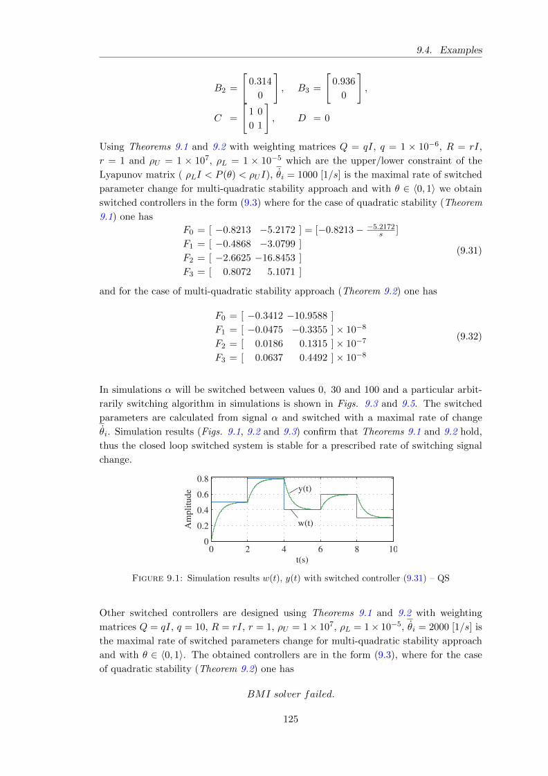
9.4. Examples
B2 =
[0.314
0
], B3 =
[0.936
0
],
C =
[1 0
0 1
], D = 0
Using Theorems 9.1 and 9.2 with weighting matrices Q = qI, q = 1 × 10⁻⁶, R = rI,
r = 1 and ρU = 1 × 10⁷, ρL = 1 × 10⁻⁵ which are the upper/lower constraint of the
Lyapunov matrix ( ρLI < P (θ) < ρUI), θi = 1000 [1/s] is the maximal rate of switched
parameter change for multi-quadratic stability approach and with θ ∈ 〈0, 1〉 we obtain
switched controllers in the form (9.3) where for the case of quadratic stability (Theorem
9.1) one has
F0 = [ −0.8213 −5.2172 ] = [−0.8213− −5.2172s ]
F1 = [ −0.4868 −3.0799 ]
F2 = [ −2.6625 −16.8453 ]
F3 = [ 0.8072 5.1071 ]
(9.31)
and for the case of multi-quadratic stability approach (Theorem 9.2) one has
F0 = [ −0.3412 −10.9588 ]
F1 = [ −0.0475 −0.3355 ]× 10−8
F2 = [ 0.0186 0.1315 ]× 10−7
F3 = [ 0.0637 0.4492 ]× 10−8
(9.32)
In simulations α will be switched between values 0, 30 and 100 and a particular arbit-
rarily switching algorithm in simulations is shown in Figs. 9.3 and 9.5. The switched
parameters are calculated from signal α and switched with a maximal rate of change
θi. Simulation results (Figs. 9.1, 9.2 and 9.3) confirm that Theorems 9.1 and 9.2 hold,
thus the closed loop switched system is stable for a prescribed rate of switching signal
change.
Figure 9.1: Simulation results w(t), y(t) with switched controller (9.31) – QS
Other switched controllers are designed using Theorems 9.1 and 9.2 with weighting
matrices Q = qI, q = 10, R = rI, r = 1, ρU = 1× 10⁷, ρL = 1× 10⁻⁵, θi = 2000 [1/s] is
the maximal rate of switched parameters change for multi-quadratic stability approach
and with θ ∈ 〈0, 1〉. The obtained controllers are in the form (9.3), where for the case
of quadratic stability (Theorem 9.2) one has
BMI solver failed.
125
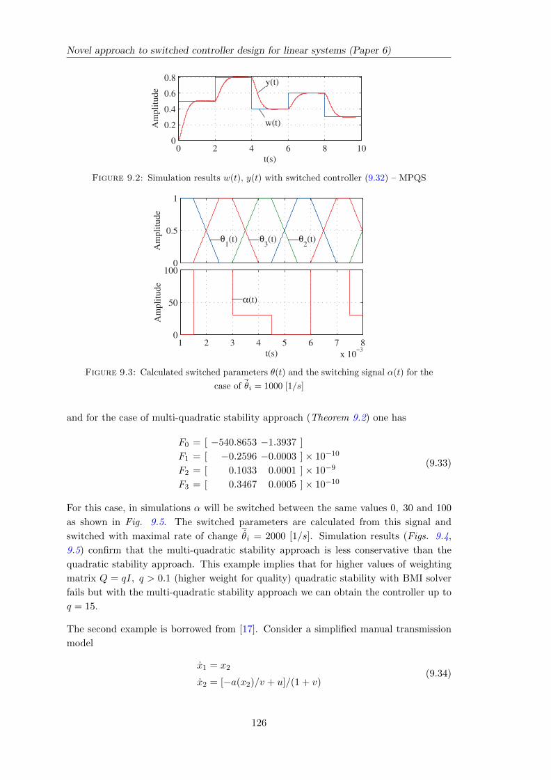
Novel approach to switched controller design for linear systems (Paper 6)
Figure 9.2: Simulation results w(t), y(t) with switched controller (9.32) – MPQS
Figure 9.3: Calculated switched parameters θ(t) and the switching signal α(t) for the
case of θi = 1000 [1/s]
and for the case of multi-quadratic stability approach (Theorem 9.2) one has
F0 = [ −540.8653 −1.3937 ]
F1 = [ −0.2596 −0.0003 ]× 10−10
F2 = [ 0.1033 0.0001 ]× 10−9
F3 = [ 0.3467 0.0005 ]× 10−10
(9.33)
For this case, in simulations α will be switched between the same values 0, 30 and 100
as shown in Fig. 9.5. The switched parameters are calculated from this signal and
switched with maximal rate of change θi = 2000 [1/s]. Simulation results (Figs. 9.4,
9.5) confirm that the multi-quadratic stability approach is less conservative than the
quadratic stability approach. This example implies that for higher values of weighting
matrix Q = qI, q > 0.1 (higher weight for quality) quadratic stability with BMI solver
fails but with the multi-quadratic stability approach we can obtain the controller up to
q = 15.
The second example is borrowed from [17]. Consider a simplified manual transmission
model
x1 = x2
x2 = [−a(x2)/v + u]/(1 + v)(9.34)
126
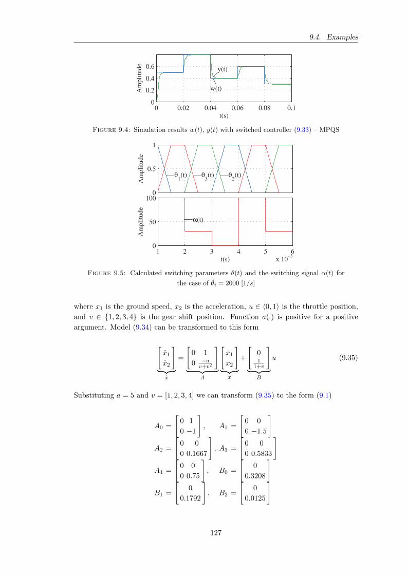
9.4. Examples
Figure 9.4: Simulation results w(t), y(t) with switched controller (9.33) – MPQS
Figure 9.5: Calculated switching parameters θ(t) and the switching signal α(t) for
the case of θi = 2000 [1/s]
where x1 is the ground speed, x2 is the acceleration, u ∈ 〈0, 1〉 is the throttle position,
and v ∈ 1, 2, 3, 4 is the gear shift position. Function a(.) is positive for a positive
argument. Model (9.34) can be transformed to this form
[x1
x2
]︸ ︷︷ ︸
x
=
[0 1
0 −av+v2
]︸ ︷︷ ︸
A
[x1
x2
]︸ ︷︷ ︸
x
+
[01
1+v
]︸ ︷︷ ︸
B
u (9.35)
Substituting a = 5 and v = [1, 2, 3, 4] we can transform (9.35) to the form (9.1)
A0 =
[0 1
0 −1
], A1 =
[0 0
0 −1.5
]
A2 =
[0 0
0 0.1667
], A3 =
[0 0
0 0.5833
]
A4 =
[0 0
0 0.75
], B0 =
[0
0.3208
]
B1 =
[0
0.1792
], B2 =
[0
0.0125
]
127
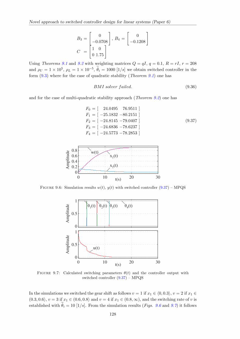
Novel approach to switched controller design for linear systems (Paper 6)
B3 =
[0
−0.0708
], B4 =
[0
−0.1208
]
C =
[1 0
0 1.75
]Using Theorems 9.1 and 9.2 with weighting matrices Q = qI, q = 0.1, R = rI, r = 208
and ρU = 1 × 10⁵, ρL = 1 × 10⁻⁵, θi = 1000 [1/s] we obtain switched controller in the
form (9.3) where for the case of quadratic stability (Theorem 9.1) one has
BMI solver failed. (9.36)
and for the case of multi-quadratic stability approach (Theorem 9.2) one has
F0 = [ 24.0495 76.9511 ]
F1 = [ −25.1832 −80.2151 ]
F2 = [ −24.8145 −79.0407 ]
F3 = [ −24.6836 −78.6237 ]
F4 = [ −24.5773 −78.2853 ]
(9.37)
Figure 9.6: Simulation results w(t), y(t) with switched controller (9.37) – MPQS
Figure 9.7: Calculated switching parameters θ(t) and the controller output withswitched controller (9.37) – MPQS
In the simulations we switched the gear shift as follows v = 1 if x1 ∈ 〈0, 0.3〉, v = 2 if x1 ∈(0.3, 0.6〉, v = 3 if x1 ∈ (0.6, 0.8〉 and v = 4 if x1 ∈ (0.8,∞), and the switching rate of v is
established with θi = 10 [1/s]. From the simulation results (Figs. 9.6 and 9.7) it follows
128
9.4. Examples
that the theorems holds and that the multi-parameter quadratic stability approach is
less conservative than the quadratic stability and that with the weighting matrices we
can affect the performance quality and tune the system to the desired conditions.
Third example. Control systems over data networks are commonly referred to as net-
worked control systems (NCSs). For the NCSs, the sampled data and controller signals
are transmitted through a network. As a result, it leads to a network-induced delay
in a networked control closed-loop system. The existence of such a kind of delay in a
network-based control loop can induce instability or poor performance of control sys-
tems. Assume that a linear system with transfer function G(s) is integrated to NCSs
which inevitably leads to a change of the plant transfer function as G(s)e−Tds, where Tdis a variable plant time delay. The value of Td depends on the load of the communication
network. Assume that for four communication network loads one can define four middle
values of time delays Tdi, i = 1, 2, 3, 4.
For PI switched controller design and simulation we will use a laboratory model of a
DC-motor which is one of the real processes built for control education and research
at our institute. We have identified the DC motor system and the following transfer
function has been obtained
Sys =0.0627s+ 1.281
2.081s2 + 2.506s+ 1(9.38)
For the defined 4 middle values of the induced time delays Td = [0.1, 0.2, 0.3, 0.4] s and
using the first order Pade approximation we computed 4 plant transfer functions which
are transformed to the state space. The obtained 4 plant models are extended with one
state for the switched PI controller design. Finally one obtains the plant models in the
form (9.1)
A0 =
0 1 0 0
0 0 1 0
−5.0006 −13.0218 −11.6208 0
1 0 0 0
, A1 =
0 0 0 0
0 0 0 0
−4.6005 −11.5382 −9.5832 0
0 0 0 0
A2 =
0 0 0 0
0 0 0 0
0.2001 0.5018 0.4168 0
0 0 0 0
, A3 =
0 0 0 0
0 0 0 0
1.8001 4.5147 3.7498 0
0 0 0 0
A4 =
0 0 0 0
0 0 0 0
2.6003 6.5218 5.4168 0
0 0 0 0
, B0 =
−0.0308
0.0498
4.1652
0
, B1 =
−0.0002
0.5833
−4.5362
0
B2 =
−0.0002
−0.0261
2.1004
0
, B3 =
0.0008
−0.2288
1.5999
0
, B4 =
−0.0003
−0.3284
0.8360
0
, C =
[1 0 0 0
0 0 0 1
]
129
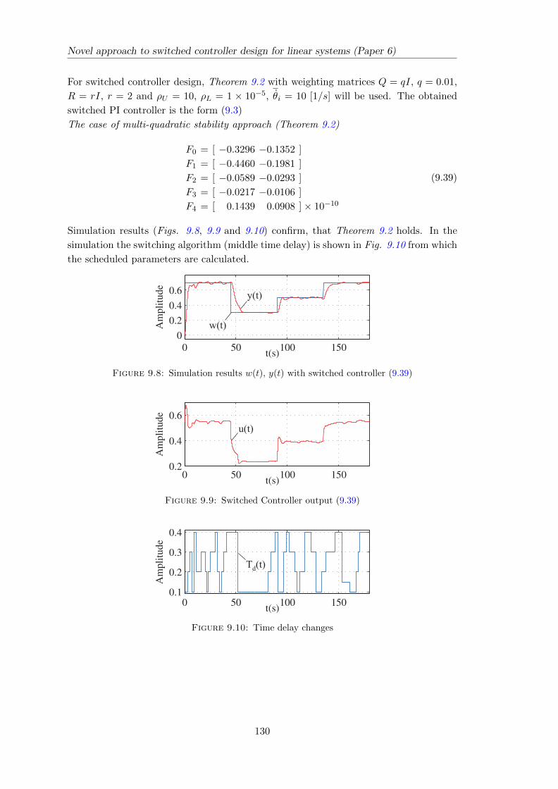
Novel approach to switched controller design for linear systems (Paper 6)
For switched controller design, Theorem 9.2 with weighting matrices Q = qI, q = 0.01,
R = rI, r = 2 and ρU = 10, ρL = 1 × 10⁻⁵, θi = 10 [1/s] will be used. The obtained
switched PI controller is the form (9.3)
The case of multi-quadratic stability approach (Theorem 9.2)
F0 = [ −0.3296 −0.1352 ]
F1 = [ −0.4460 −0.1981 ]
F2 = [ −0.0589 −0.0293 ]
F3 = [ −0.0217 −0.0106 ]
F4 = [ 0.1439 0.0908 ]× 10−10
(9.39)
Simulation results (Figs. 9.8, 9.9 and 9.10) confirm, that Theorem 9.2 holds. In the
simulation the switching algorithm (middle time delay) is shown in Fig. 9.10 from which
the scheduled parameters are calculated.
Figure 9.8: Simulation results w(t), y(t) with switched controller (9.39)
Figure 9.9: Switched Controller output (9.39)
Figure 9.10: Time delay changes
130
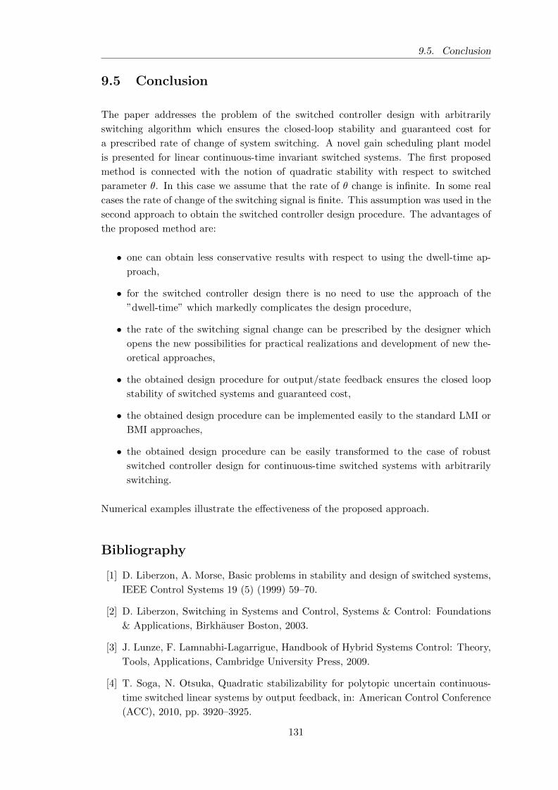
9.5. Conclusion
9.5 Conclusion
The paper addresses the problem of the switched controller design with arbitrarily
switching algorithm which ensures the closed-loop stability and guaranteed cost for
a prescribed rate of change of system switching. A novel gain scheduling plant model
is presented for linear continuous-time invariant switched systems. The first proposed
method is connected with the notion of quadratic stability with respect to switched
parameter θ. In this case we assume that the rate of θ change is infinite. In some real
cases the rate of change of the switching signal is finite. This assumption was used in the
second approach to obtain the switched controller design procedure. The advantages of
the proposed method are:
• one can obtain less conservative results with respect to using the dwell-time ap-
proach,
• for the switched controller design there is no need to use the approach of the
”dwell-time” which markedly complicates the design procedure,
• the rate of the switching signal change can be prescribed by the designer which
opens the new possibilities for practical realizations and development of new the-
oretical approaches,
• the obtained design procedure for output/state feedback ensures the closed loop
stability of switched systems and guaranteed cost,
• the obtained design procedure can be implemented easily to the standard LMI or
BMI approaches,
• the obtained design procedure can be easily transformed to the case of robust
switched controller design for continuous-time switched systems with arbitrarily
switching.
Numerical examples illustrate the effectiveness of the proposed approach.
Bibliography
[1] D. Liberzon, A. Morse, Basic problems in stability and design of switched systems,
IEEE Control Systems 19 (5) (1999) 59–70.
[2] D. Liberzon, Switching in Systems and Control, Systems & Control: Foundations
& Applications, Birkhauser Boston, 2003.
[3] J. Lunze, F. Lamnabhi-Lagarrigue, Handbook of Hybrid Systems Control: Theory,
Tools, Applications, Cambridge University Press, 2009.
[4] T. Soga, N. Otsuka, Quadratic stabilizability for polytopic uncertain continuous-
time switched linear systems by output feedback, in: American Control Conference
(ACC), 2010, pp. 3920–3925.
131
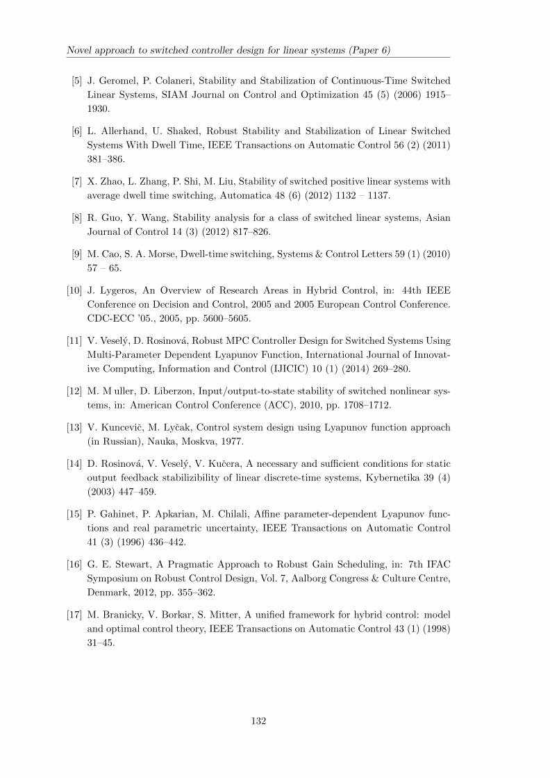
Novel approach to switched controller design for linear systems (Paper 6)
[5] J. Geromel, P. Colaneri, Stability and Stabilization of Continuous-Time Switched
Linear Systems, SIAM Journal on Control and Optimization 45 (5) (2006) 1915–
1930.
[6] L. Allerhand, U. Shaked, Robust Stability and Stabilization of Linear Switched
Systems With Dwell Time, IEEE Transactions on Automatic Control 56 (2) (2011)
381–386.
[7] X. Zhao, L. Zhang, P. Shi, M. Liu, Stability of switched positive linear systems with
average dwell time switching, Automatica 48 (6) (2012) 1132 – 1137.
[8] R. Guo, Y. Wang, Stability analysis for a class of switched linear systems, Asian
Journal of Control 14 (3) (2012) 817–826.
[9] M. Cao, S. A. Morse, Dwell-time switching, Systems & Control Letters 59 (1) (2010)
57 – 65.
[10] J. Lygeros, An Overview of Research Areas in Hybrid Control, in: 44th IEEE
Conference on Decision and Control, 2005 and 2005 European Control Conference.
CDC-ECC ’05., 2005, pp. 5600–5605.
[11] V. Vesely, D. Rosinova, Robust MPC Controller Design for Switched Systems Using
Multi-Parameter Dependent Lyapunov Function, International Journal of Innovat-
ive Computing, Information and Control (IJICIC) 10 (1) (2014) 269–280.
[12] M. M uller, D. Liberzon, Input/output-to-state stability of switched nonlinear sys-
tems, in: American Control Conference (ACC), 2010, pp. 1708–1712.
[13] V. Kuncevic, M. Lycak, Control system design using Lyapunov function approach
(in Russian), Nauka, Moskva, 1977.
[14] D. Rosinova, V. Vesely, V. Kucera, A necessary and sufficient conditions for static
output feedback stabilizibility of linear discrete-time systems, Kybernetika 39 (4)
(2003) 447–459.
[15] P. Gahinet, P. Apkarian, M. Chilali, Affine parameter-dependent Lyapunov func-
tions and real parametric uncertainty, IEEE Transactions on Automatic Control
41 (3) (1996) 436–442.
[16] G. E. Stewart, A Pragmatic Approach to Robust Gain Scheduling, in: 7th IFAC
Symposium on Robust Control Design, Vol. 7, Aalborg Congress & Culture Centre,
Denmark, 2012, pp. 355–362.
[17] M. Branicky, V. Borkar, S. Mitter, A unified framework for hybrid control: model
and optimal control theory, IEEE Transactions on Automatic Control 43 (1) (1998)
31–45.
132
10
Robust Switched Controller Design
for Nonlinear Continuous Systems
(Paper 7)
Abstract
A novel approach is presented to robust switched controller design for nonlinear
continuous-time systems under an arbitrary switching signal using the gain schedul-
ing approach. The proposed design procedure is based on the robust multi parameter
dependent quadratic stability condition. The obtained switched controller design pro-
cedure for nonlinear continuous-time systems is in at bilinear matrix form (BMI). The
properties of the obtained design are illustrated on simulation examples.
Keywords: Robust controller, Switched controller, Gain-scheduled controller, Continu-
ous time Nonlinear systems, Lyapunov function.
10.1 Introduction
Switched systems play an important role in the past decade. Motivation for studying
switched systems stems from two facts
• switched systems have numerous application in the control of real plants, and
• in real control, there are dynamical systems that cannot be stabilized by any
continuous static output/state feedback control law, but a stabilizing switching
control scheme can be found.
Therefore switched system stability and the controller design procedure are the most
important issues, especially for nonlinear systems. Stability under arbitrary switching
133
Robust Switched Controller Design for Nonlinear Continuous Systems
is guaranteed by the existence of a common Lyapunov function for all switching subsys-
tems, [1], [2], [3], [4], [5], [6]. For switched linear systems, finding the common Lyapunov
function is relatively easy but for nonlinear systems it is difficult. A survey of switched
controller design for nonlinear systems can be found in [1], [2], [3], [7] and references
therein. Due to the switched controller design problems for continuous time nonlin-
ear systems in this paper we pursue the idea to use, instead of a nonlinear switched
plant model a switched gain-scheduled plant model and to design the robust switched
gain-scheduled controller guaranteeing closed-loop stability and guaranteed cost for all
operating points of the switched nonlinear system.
Gain scheduling control deals with systems subject to parametric variations, which in-
clude linear systems with time-varying parameters or nonlinear systems modeled by a
family of linear parameter-varying systems, [8]. Because of time-varying gain-scheduled
parameters many researches have tackled the design problem of the gain-scheduled con-
trollers for linear time-varying system (LPV) using linear matrix inequalities (LMI)
and the Lyapunov function approach [8], [9], [10], [11]. Reviews of the gain-scheduled
controller design can be found in [12], [13].
In this paper a method is proposed of robust switched controller design for nonlinear
continuous time switched systems using the gain scheduling approach. There are only
some results in the field of continuous time switched gain-scheduled controller design for
continuous time systems [14], [15], [16] and stabilization of switched continuous time lin-
ear systems [17], [18]. Representative are two last references [17], [18]. In the first paper
the authors introduce the notion of the dwell-time Td (minimal time interval between
switching) into the switched controller design procedure. In the stability analysis con-
dition of switched systems the dwell-time is included to the term eAcTd (Ac-closed-loop
matrix (10.4)). In such a way the proposed design procedure for stability analysis and
switching controller design for the real switching time interval T > Td becomes conservat-
ive. The ”dwell-time term” for continuous-time systems very complicated the switched
controller design procedure. In the paper [18] sufficient conditions are given for the sta-
bility of linear systems with dwell-time and with polytopic type parameter uncertainty.
Lyapunov functions, in quadratic form for each mode, which are non-increasing at the
switching instants are assigned to each mode. During the dwell-time this function varies
piecewise linearly in time after switching occurs. The proposed method was applied to
stabilization via a state feedback both for nominal and uncertain cases. Since within the
dwell-time the Lyapunov function varies piecewise linearly and the real switching time
interval T > Td, the switching controller design procedure become rather conservative.
The switched controller design procedure for continuous-time systems proposed in this
paper does not use the approach of the ”dwell-time”, therefore there is no such drawback
as mentioned in the above references.
Vast references on the switched controller design are concentrated on the case where
switching can occur immediately (ideal case), for a large number of switched system the
realistic case is where the rate of change of the switching signal is finite (non-ideal case).
A assumption of a non-ideal case of the switching variable will be used in this paper
which gives other opportunities for controller designer. Some results about the stability
134
10.2. Problem statement and preliminaries
of a class of uncertain linear varying systems (transform to switched systems) can be
found in [19].
The remainder of the paper is organized as follows. In Section 10.1 and 10.2 we present
the class of switched gain-scheduled control systems. In Section 10.3 we address the
output feedback PI switched gain-scheduled robust controller design procedure for con-
tinuous time gain-scheduled plant model. Finally, in Section 10.4, the proposed design
procedure is demonstrated on a simple example.
Our notation is standard, P ∈ Rm×n denotes the set of real m × n matrices, P > 0
(P ≥ 0) ∈ Rn×n is a real symmetric, positive definite (semidefinite) matrix. σ ∈ S
indicates the arbitrary switching algorithm and σ + 1 is the first next mode to mode
σ. ”*” in matrices denotes the respective transposed (conjugate) term to make matrix
symmetric. Im is an m×m identity matrix, 0m denotes the zero matrix.
10.2 Problem statement and preliminaries
10.2.1 Uncertain LPV plant model for switched systems
Consider family of nonlinear switched systems
z = fσ(z, v, w) σ ∈ S = 1, 2, . . . , Ny = h(z)
(10.1)
where z ∈ Rn is the state, the input v ∈ Rm, the output y ∈ Rl, exogenous input w ∈ Rk
which captures parametric dependence of the plant (10.1) on exogenous input. The
arbitrary switching algorithm σ ∈ S is a piecewise constant, right continuous function
which specifies at each time the index of the active system, [20]. Assume that f(.) is
locally Lipschitz for every σ ∈ S. Consider that the number of equilibrium points for
each switching modes is equal to p, that is for each mode σ ∈ S the nonlinear system can
be replaced by a family of p linearized plant. For more details how to obtain the gain-
scheduled plant model see excellent surveys [12], [13]. To receive the model uncertainty of
the gain-scheduled plant it is necessary to obtain other family of linearized plant models
around the p equilibrium points. Finally, one obtains the gain-scheduled uncertain plant
model in the form
x = Aσ(ξ, θ)x+Bσ(ξ, θ)u σ ∈ Sy = Cx
(10.2)
where x = z − ze, u = v − ve, y = y − ye, (ze, ve, ye) define the equilibrium family for
plant (10.1). Assume, that for i − th equilibrium point one obtain the sets x ∈ Xi,
u ∈ Ui, y ∈ Yi, i = 1, 2, . . . , p. Summarizing above sets we get x ∈ X =⋃pi=1Xi, u ∈
135
Robust Switched Controller Design for Nonlinear Continuous Systems
U =⋃pi=1 Ui, y ∈ Y =
⋃pi=1 Yi.
Aσ(ξ, θ) = Aσ0(ξ) +
p∑j=1
Aσj(ξ)θj ∈ Rn×n
Bσ(ξ, θ) = Bσ0(ξ) +
p∑j=1
Bσj(ξ)θj ∈ Rn×m(10.3)
Matrices Aσj(ξ), Bσj(ξ), j = 0, 1, 2, . . . , p belong to the convex set a polytope with K
vertices that can formally defined as
Ωσ =
Aσj(ξ), Bσj(ξ) =
K∑i=1
(Aσij , Bσij) ξi
j = 0, 1, 2, 3, . . . , p,
K∑i=1
ξi = 1, ξi ≥ 0, ξi ∈ Ωξ
(10.4)
where ξi, i = 1, 2, . . . ,K are constant or possible time-varying but unknown parameters,
Aσij , Bσij , C are constant matrices of corresponding dimensions, θ ∈ Rp is a vector of
known constant or time-varying gain-scheduled parameter. Assume that both lower and
upper bounds are available, that is
θ ∈ Ωs = θ ∈ Rp : θj ∈ 〈θj , θj〉θ ∈ Ωt = θ ∈ Rp : θj ∈ 〈θj , θj〉
(10.5)
10.2.2 Problem formulation
For each plant mode consider the uncertain gain-scheduled LPV plant model in the form
(10.2), (10.3) and (10.4)
x =
Aσ0(ξ) +
p∑j=1
Aσj(ξ)θj
x+
Bσ0(ξ) +
p∑j=1
Bσj(ξ)θj
u
y = Cx
(10.6)
For a robust gain-scheduled I part controller design, the states x of (10.6) need to
be extended in such a way that a static output feedback control algorithm can provide
proportional (P) and integral (I) parts of the designed controller, for more detail see [21].
Assume that system (10.6) allows PI controller design with a static output feedback. The
feedback control law is considered in the form
u = Fσ(θ)y =
Fσ0 +
p∑j=1
Fσjθj
Cx (10.7)
where Fσ(θ) is the static output feedback gain-scheduled controller for mode σ. The
closed-loop system is
x = Aσc(ξ, θ, α)x (10.8)
136

10.3. Main results
where
Aσc(ξ, θ, α) =
N∑σ=1
(Aσ(ξ, θ) +Bσ(ξ, θ)Fσ(θ)C
)ασ =
N∑σ=1
Aσ(ξ, θ)ασ
αT = [α1, α2, . . . , αN ],N∑σ=1
ασ = 1,N∑σ=1
ασ = 0
αj = 1 when σj is active plant mode, else αj = 0. Assume α ∈ Ωα, α ∈ Ωd.
To access the system performance, we consider an original weighted scheduled quadratic
cost function
J =
∫ ∞t=0
J(t)dt (10.9)
where J(t) = xTQ(θ)x+ uTRu and
Q(θ) = Q0 +
p∑j=1
Qjθj , Qj ≥ 0, R > 0
.
Definition 10.1. Consider a stable closed-loop switched system (10.8) with N modes.
If there is a control algorithm (10.7) and a positive scalar J∗ such that the closed-loop
cost function (10.9) satisfies J ≤ J∗ for all θ ∈ Ωs, α ∈ Ωα, then J∗ is said to be a
guaranteed cost and ”u” is said to be a guaranteed cost control algorithm for arbitrary
switching algorithm σ ∈ S.
Theorem 10.1. [22] Control algorithm (10.7) is the guaranteed cost control law
for the switched closed-loop system (10.8) if and only if there is Lyapunov function
V (x, ξ, θ, α) > 0, matrices Q(θ), R and gain matrices Fσk, k = 0, 1, . . . , p such that for
σ ∈ S the following inequality holds
Be =dV (x, ξ, θ, α)
dt+ J(t) ≤ −εxTx, ε→ 0 (10.10)
10.3 Main results
This section formulates the theoretical approach to the robust switched gain-scheduled
controller design with control law (10.7) which ensure closed-loop multi parameter de-
pendent quadratic stability and guaranteed cost for an arbitrary switching algorithm
σ ∈ S. Assume that in Theorem 10.1 the Lyapunov function is in the form
V (x, ξ, θ, α) = xTP (ξ, θ, α)x (10.11)
where the Lyapunov multi parameter-dependent matrix is
P (ξ, θ, α) =
K∑i=1
P0i +
N∑σ=1
Pσ0i +
p∑j=1
Pσijθj
ασ
ξi (10.12)
137
Robust Switched Controller Design for Nonlinear Continuous Systems
Time derivative of the Lyapunov function(10.11) is
V (.) = [xT xT ]
[0 P (ξ, θ, α)
P (ξ, θ, α) P (ξ, θ, α)
][x
x
](10.13)
where
P (.) =K∑i=1
N∑σ=1
DPσiασξi (10.14)
DPσi =
N∑σ=1
Pσ0iασ +
p∑j=1
Pσij θj +
p∑j=1
N∑σ=1
Pσijασθj
Using equality
(2N1x+ 2N2x)T
(x−
N∑σ=1
Aσ(ξ, θ)ασx
)= 0 (10.15)
equation (10.13) can be rewritten as
dV (.)
dt=
N∑σ=1
[xT xT
]Lσ(ξ, θ)
[x
x
](10.16)
Lσ(ξ, θ) = lσ(i, j)2×2
lσ(1, 1) = NT1 +N1
lσ(1, 2) = −NT1 Aσ(ξ, θ) +N2 +
K∑i=1
P0i + Pσ0i +
p∑j=1
Pσijθj
ξi
lσ(2, 2) = −NT2 Aσ(ξ, θ)−ATσ (ξ, θ)N2 +
K∑i=1
DPσiξi
where N1, N2 ∈ Rn×n are auxiliary matrices.
On substituting (10.7) to (10.9) one obtains
J(t) = xTS(θ)x (10.17)
where
S(θ) = S0 +
p∑j=1
Sjθj +
p∑j=1
p∑k>j
Skjθkθj +
p∑k=1
Skkθ2k
S0 = Q0 + CTF Tσ0RFσoC
Sj = Qj + CT(F Tσ0RFσj + F TσjRFσ0
)C
Sjk = CT(F TσjRFσk + F TσkRFσj
)C
Skk = CTF TσkRFσkC
138
10.3. Main results
The switched model plant (10.8) can be rewritten to the form
Aσ(ξ, θ) = M0(ξ) +
p∑j=1
Mj(ξ)θj +
p∑j=1
p∑k>j
Mjk(ξ)θjθk+ (10.18)
p∑k
Mkk(ξ)θ2
where
M0(ξ) = Aσ0(ξ) +Bσ0(ξ)Fσ0C
Mj(ξ) = Aσj + (Bσ0(ξ)Fσj +Bσj(ξ)Fσ0)C
Mjk(ξ) = (Bσj(ξ)Fσk +Bσk(ξ)Fσj)C
Mkk(ξ) = Bσk(ξ)FσkC
Due to Theorem 10.1 the closed-loop switched gain-scheduled system is multi parameter
dependent quadratically stable with guaranteed cost for σ ∈ S, ξi, i = 1, 2, . . . ,K if the
following inequalities hold
Be = [xT xT ]W (ξ, σ, θ)[xT xT ]T ≤ 0 (10.19)
where W (ξ, σ, θ) = wij(σ, ξ)2×2
w11(σ, ξ) = NT1 +N1
w12(σ, ξ) =∑K
i=1
(P0i + Pσ0i +
∑pj=1 Pσijθj
)ξi
− NT1 Aσ(ξ, θ) +N2
w22(σ, ξ) = −NT2 Aσ(ξ, θ)−Aσ(ξ, θ)TN2
+∑K
i=1DPσiξi + S(θ)
Inequality (10.19) implies :
• for all σ ∈ S the inequality is linear with respect to uncertain parameter ξi,
i = 1, 2, . . . ,K,
• for all σ ∈ S the inequality is a quadratic function with respect to the gain-
scheduled parameters θi, i = 1, 2, . . . , p.
For the next development the following theorem is useful.
Theorem 10.2. [23] Consider a scalar quadratic function of θ ∈ Rp
f(θ) = a0 +
p∑j=1
ajθj +
p∑j=1
p∑k>j
ajkθjθk +
p∑k
akkθ2k (10.20)
139
Robust Switched Controller Design for Nonlinear Continuous Systems
and assume that if f(θ) is multiconvex, that is
δ2f(θ)
δθ2k
= 2akk ≥ 0, k = 1, 2, . . . , p
then f(θ) is negative definite in the hyper rectangle (10.5) if and only if it takes negative
values at the vertices of (10.5), that is if and only if f(θ) < 0 for all vertices of the set
given by (10.5).
Due to (10.14), (10.17) and (10.18) the robust stability conditions of switched system
can be rewritten as
W (ξ, σ, θ) =
N∑σ=1
L(θ, ξ)ασ =
N∑σ=1
(Wσ0(ξ)+
+
p∑j=1
Wσj(ξ)θj +
p∑j=1
p∑k>j
Wσjk(ξ)θjθk+
+
p∑k=1
Wσkkθ2k)ασ ≤ 0
(10.21)
where Wσ0(ξ) = wσ0ij2×2, Wσj(ξ) = wσjik2×2
wσ011 = NT1 +N1
wσ012 = −NT1 M0(ξ) +N2 +
∑Ki=1(P0i + Pσ0i)ξi
wσ022 = −NT2 M0(ξ)−MT
0 (ξ)N2 + S0+
+∑K
i=1
(Pσ0iασ +
∑pj=1 Pσij θj
)ξi
wσj11 = 0; wσj12 = −NT1 Mj(ξ) +
∑Ki=1 Pσijξi
wσj22 = −NT2 Mj(ξ)−Mj(ξ)
TN2 + Sj+
+∑K
i=1
(∑Nσ=1 Pσijασ
)ξi
Wσjk(ξ) =
[0 −NT
1 Mjk(ξ)” ∗ ” −NT
2 Mjk(ξ)−Mjk(ξ)TN2 + Sjk
]Wσkk(ξ) =
[0 −NT
1 Mkk(ξ)” ∗ ” −NT
2 Mkk(ξ)−Mkk(ξ)TN2 + Skk
]The main results on the robust stability condition for the switched gain-scheduled control
system is given in the next theorem.
Theorem 10.3. Closed-loop switched system (10.8) is robust multi parameter dependent
quadratically stable with guaranteed cost if there is a positive definite matrix P (ξ, θ, α) ∈Rn×n (10.12), matrices N1, N2 ∈ Rn×n, positive definite (semidefinite) matrices Q(θ),
R and gain-scheduled controller matrix Fσ(θ), such that for σ ∈ S
1.
Lσ(ξ, θ) < 0 (10.22)
140
10.4. Example
2.
Wσkk ≥ 0, σ ∈ S, θ ∈ Ωs, k = 1, 2, . . . , p
The proof of theorem sufficient conditions immediately follows from eqs. (10.12)-(10.21).
Notes.
• Lσ(θ, ξ) is linear with respect to uncertain parameter ξi, i = 1, 2, . . . ,K, it holds
Lσ(θ, ξ) =∑K
i=1 Lσi(θ)ξi, therefore inequality (10.22) for each σ ∈ S split to K
inequalities of type Lσi(θ) < 0 and Wσikk ≥ 0.
• Eq. (10.12) implies that in dependence on the chosen structure of the Lyapunov
matrix P (ξ, θ, α) one should obtained different types of stability conditions from
quadratic to multi parameter dependent quadratic stabilities. Different types of
stability conditions determine the conservatism of the design procedure and the
rate of change of corresponding variables.
10.4 Example
Consider a simple nonlinear switched system with two modes as
σ = 1, x = −asinx+ bu
σ = 2, x = −acosx+ bu, y = x(10.23)
where a ∈ 〈0.8, 1〉, when a = 0.8 then b = 1 and a = 1, b = 0.5. One can linearized
model (10.23) in the three working points x0 = 0, π/4, π/2. For PI gain-scheduled
controller design the system state space needs to be increased, finally for matrices
A(σ, ξ, θ), B(σ, ξ, θ) one obtains
A(1, ξ, θ) =
[−0.4 0
1 0
]+
[0.117 0
0 0
]θ1 +
[−0.28 0
0 0
]θ2
ξ1
+
[−0.5 0
1 0
]+
[0.14645 0
0 0
]θ1 +
[−0.35355 0
0 0
]θ2
ξ2
B(1, ξ, θ) =
[10
]ξ1 +
[0.50
]ξ2
(10.24)
A(2, ξ, θ) =
[0.4 01 0
]+
[−0.287 0
0 0
]θ1 +
[−0.117 0
0 0
]θ2
ξ1
+
[0.5 01 0
]+
[−.35955 0
0 0
]θ1 +
[−0.14645 0
0 0
]θ2
ξ2
B(2, ξ, θ) =
[10
]ξ1 +
[0.50
]ξ2
(10.25)
C =
[1 00 1
]
141
Robust Switched Controller Design for Nonlinear Continuous Systems
For each mode, the robust gain-scheduled controller has been designed for the following
parameters Q0 = 0.01∗ I, Q1 = 0.001∗ I, Q2 = 0.005∗ I, R = I, max ασ = 1001s (rate of
switching parameters changing) max θj = 11s maximal rate of gain-scheduled parameter
changes. Constraints for the Lyapunov matrix (10.12) are 0 < P (ξ, θ, α) < 1000 ∗ I.
The obtained first gain-scheduled controller parameters are:
σ = 1
R1 = −7.8434− 3.852
s+
−4.794− 2.6287
s
θ1
+
0.3278 +
0.866
s
θ2
σ = 2
R2 = −13.8691− 6.3453
s+
−8.0619− 4.7241
s
θ1
+ 0.4297 +1.2511
sθ2
(10.26)
The maximal closed-loop eigenvalues for the case of θj = 0, j = 1, 2, . . . , p are
σ = 1,maxeig(CLS) = −0.4899
σ = 2,maxeig(CLS) = −0.4888
Under the same conditions other results have been obtained for the case of
max ασ = 300/s and max θj = 5/s. The second gain-scheduled controller para-
meters are:
σ = 1
R1 = −7.1769− 2.0309
s+
−1.2374 +
2.4355
s
θ1
+
4.9032− 2.7108
s
θ2
(10.27)
σ = 2
R2 = −3.9991− 1.7337
s+
−02912 +
1.3464
s
θ1
+
1.1521− 1.4535
s
θ2
(10.28)
The maximal closed-loop eigenvalues for the case of θj = 0, j = 1, 2, . . . , p are
σ = 1,maxeig(CLS) = −0.2656
σ = 2,maxeig(CLS) = −0.5729
Note that the negative sign means a negative feedback. Simulation results for the two
designed gain-scheduled switched controller are given in Figs. 10.1-10.6
142
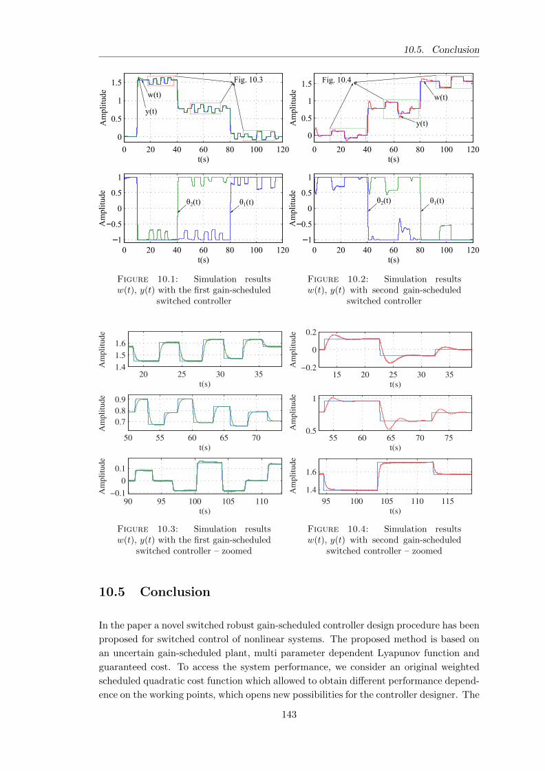
10.5. Conclusion
0 20 40 60 80 100 120
0
0.5
1
1.5
t(s)
Am
pli
tud
e
0 20 40 60 80 100 120
1
0.5
0
0.5
1
t(s)
Am
pli
tud
e
Fig. 10.3
w(t)
y(t)
θ2(t) θ1(t)
Figure 10.1: Simulation resultsw(t), y(t) with the first gain-scheduled
switched controller
0 20 40 60 80 100 120
0
0.5
1
1.5
t(s)
Am
pli
tud
e
0 20 40 60 80 100 120
1
0.5
0
0.5
1
t(s)
Am
pli
tud
e
w(t)
y(t)
Fig. 10.4
θ2(t) θ1(t)
Figure 10.2: Simulation resultsw(t), y(t) with second gain-scheduled
switched controller
Figure 10.3: Simulation resultsw(t), y(t) with the first gain-scheduled
switched controller – zoomed
Figure 10.4: Simulation resultsw(t), y(t) with second gain-scheduled
switched controller – zoomed
10.5 Conclusion
In the paper a novel switched robust gain-scheduled controller design procedure has been
proposed for switched control of nonlinear systems. The proposed method is based on
an uncertain gain-scheduled plant, multi parameter dependent Lyapunov function and
guaranteed cost. To access the system performance, we consider an original weighted
scheduled quadratic cost function which allowed to obtain different performance depend-
ence on the working points, which opens new possibilities for the controller designer. The
143
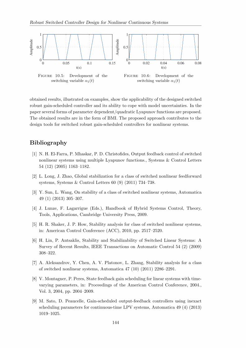
Robust Switched Controller Design for Nonlinear Continuous Systems
Figure 10.5: Development of theswitching variable α1(t)
Figure 10.6: Development of theswitching variable α1(t)
obtained results, illustrated on examples, show the applicability of the designed switched
robust gain-scheduled controller and its ability to cope with model uncertainties. In the
paper several forms of parameter dependent/quadratic Lyapunov functions are proposed.
The obtained results are in the form of BMI. The proposed approach contributes to the
design tools for switched robust gain-scheduled controllers for nonlinear systems.
Bibliography
[1] N. H. El-Farra, P. Mhaskar, P. D. Christofides, Output feedback control of switched
nonlinear systems using multiple Lyapunov functions., Systems & Control Letters
54 (12) (2005) 1163–1182.
[2] L. Long, J. Zhao, Global stabilization for a class of switched nonlinear feedforward
systems, Systems & Control Letters 60 (9) (2011) 734–738.
[3] Y. Sun, L. Wang, On stability of a class of switched nonlinear systems, Automatica
49 (1) (2013) 305–307.
[4] J. Lunze, F. Lagarrigue (Eds.), Handbook of Hybrid Systems Control, Theory,
Tools, Applications, Cambridge University Press, 2009.
[5] H. R. Shaker, J. P. How, Stability analysis for class of switched nonlinear systems,
in: American Control Conference (ACC), 2010, pp. 2517–2520.
[6] H. Lin, P. Antsaklis, Stability and Stabilizability of Switched Linear Systems: A
Survey of Recent Results, IEEE Transactions on Automatic Control 54 (2) (2009)
308–322.
[7] A. Aleksandrov, Y. Chen, A. V. Platonov, L. Zhang, Stability analysis for a class
of switched nonlinear systems, Automatica 47 (10) (2011) 2286–2291.
[8] V. Montagner, P. Peres, State feedback gain scheduling for linear systems with time-
varying parameters, in: Proceedings of the American Control Conference, 2004.,
Vol. 3, 2004, pp. 2004–2009.
[9] M. Sato, D. Peaucelle, Gain-scheduled output-feedback controllers using inexact
scheduling parameters for continuous-time LPV systems, Automatica 49 (4) (2013)
1019–1025.
144
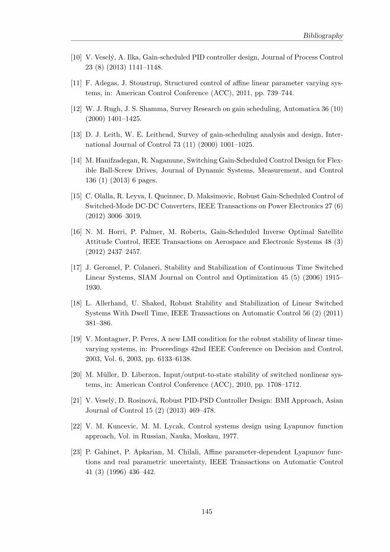
Bibliography
[10] V. Vesely, A. Ilka, Gain-scheduled PID controller design, Journal of Process Control
23 (8) (2013) 1141–1148.
[11] F. Adegas, J. Stoustrup, Structured control of affine linear parameter varying sys-
tems, in: American Control Conference (ACC), 2011, pp. 739–744.
[12] W. J. Rugh, J. S. Shamma, Survey Research on gain scheduling, Automatica 36 (10)
(2000) 1401–1425.
[13] D. J. Leith, W. E. Leithead, Survey of gain-scheduling analysis and design, Inter-
national Journal of Control 73 (11) (2000) 1001–1025.
[14] M. Hanifzadegan, R. Nagamune, Switching Gain-Scheduled Control Design for Flex-
ible Ball-Screw Drives, Journal of Dynamic Systems, Measurement, and Control
136 (1) (2013) 6 pages.
[15] C. Olalla, R. Leyva, I. Queinnec, D. Maksimovic, Robust Gain-Scheduled Control of
Switched-Mode DC-DC Converters, IEEE Transactions on Power Electronics 27 (6)
(2012) 3006–3019.
[16] N. M. Horri, P. Palmer, M. Roberts, Gain-Scheduled Inverse Optimal Satellite
Attitude Control, IEEE Transactions on Aerospace and Electronic Systems 48 (3)
(2012) 2437–2457.
[17] J. Geromel, P. Colaneri, Stability and Stabilization of Continuous Time Switched
Linear Systems, SIAM Journal on Control and Optimization 45 (5) (2006) 1915–
1930.
[18] L. Allerhand, U. Shaked, Robust Stability and Stabilization of Linear Switched
Systems With Dwell Time, IEEE Transactions on Automatic Control 56 (2) (2011)
381–386.
[19] V. Montagner, P. Peres, A new LMI condition for the robust stability of linear time-
varying systems, in: Proceedings 42nd IEEE Conference on Decision and Control,
2003, Vol. 6, 2003, pp. 6133–6138.
[20] M. Muller, D. Liberzon, Input/output-to-state stability of switched nonlinear sys-
tems, in: American Control Conference (ACC), 2010, pp. 1708–1712.
[21] V. Vesely, D. Rosinova, Robust PID-PSD Controller Design: BMI Approach, Asian
Journal of Control 15 (2) (2013) 469–478.
[22] V. M. Kuncevic, M. M. Lycak, Control systems design using Lyapunov function
approach, Vol. in Russian, Nauka, Moskau, 1977.
[23] P. Gahinet, P. Apkarian, M. Chilali, Affine parameter-dependent Lyapunov func-
tions and real parametric uncertainty, IEEE Transactions on Automatic Control
41 (3) (1996) 436–442.
145

11
Gain-Scheduled MPC Design
for Nonlinear Systems with Input
Constraints (Paper 8)
Abstract
A novel methodology is proposed for discrete model predictive gain-scheduled controller
design for nonlinear systems with input(hard)/output(soft) constraints for finite and
infinite prediction horizons. The proposed design procedure is based on the linear
parameter-varying (LPV) paradigm, affine parameter-dependent quadratic stability and
on the notion of the parameter-varying guaranteed cost. The obtained design procedure
is in the form of BMI. Numerical examples show the benefit of the proposed approach.
Keywords: Gain-scheduled controller, Predictive controller, Parameter-dependent Lya-
punov function, Quadratic gain-scheduled cost function, LPV systems, Nonlinear sys-
tems.
11.1 Introduction
The robust control theory is well established for linear systems but almost all real pro-
cesses are more or less nonlinear. If the plant operating region is small, one can use
the robust control approaches to design a linear robust controller where the nonlinear-
ities are treated as model uncertainties. However, for real nonlinear processes, where
the operating region is large, the above mentioned controller synthesis may be inap-
plicable. For this reason the controller design for nonlinear systems is nowadays a very
determinative and important field of research.
Gain scheduling is one of the most common used controller design approaches for non-
linear systems and has a wide range of use in industrial applications. Many of the
147
GS MPC Design for Nonlinear Systems with Input Constraints (Paper 8)
early articles were associated with flight control [1, 2] and aerospace [3]. Then, gradu-
ally, this approach has been used almost everywhere in control engineering, which was
greatly helped with the introduction of LPV systems. Linear parameter-varying systems
are time-varying plants whose state space matrices are fixed functions of some vector
of varying parameters θ(t). They were introduced first by Jeff S. Shamma in 1988 to
model gain scheduling. Today the LPV paradigm has become a standard formalism in
systems and controls with lot of researches and articles devoted to analysis, controller
design and system identification of these models [4].
It is known that every real system contains some constraints and it is necessary to take
account of them in the controller design procedure. The basic solution to this problem
was to include some anti-windup techniques in gain scheduling [5, 6].
A more systematic approach which allowed new possibilities is the model predictive con-
trol (MPC). That is why MPC attracted a lot of practitioners and became one of the
most used advanced control techniques in industrial applications. More information can
be found in survey [7]. The underlying idea of MPC is to use the system model to predict
the future system behaviour and then to find an optimal system input by minimization
of a cost function. Although the MPC was successfully applied to a wide range of indus-
trial processes, it contains some limitations which are caused by the drawbacks in the
MPC formulation. In the standard MPC without modifications the closed-loop stability
is not guaranteed, not mention robust stability and the computational complexity of
QP (quadratic programming) solver in each sample time and the feasibility of the cost
function with constraints. For this reason, the MPC and the nonlinear MPC has re-
ceived much attention in this research area [8, 9]. In many articles the nonlinear system
is described by LPV approximation or by gain scheduling. In paper [10] one can find a
robust output feedback MPC design for LPV systems where the control law is computed
based on LMI at each sampling time. The authors in [11] presented an observer-based
controller for nonlinear systems, where the control law is generated using the Jacobian
linearization in conjunction with gain scheduling. In paper [12] one can find a stabilizing
scheduled output feedback MPC algorithm for constrained nonlinear systems with large
operating regions, where the authors design a set of local output feedback predictive
controllers with their estimated regions of stability covering the desired operating re-
gion, then on-line switches between them with achieving the nonlinear transitions with
guaranteed stability. Another MPC algorithm can be found for LPV systems in papers
[13] and [14]. Robust output feedback MPC using off-line LMI can be found in [15] and
off-line MPC based on gain scheduling for networked control system in a brief paper
[16].
The main motivation of our paper were our previous results in gain scheduling [17], [18],
[19] and the results from a stable model predictive control design [20]. Following the
literature in this paper we have proposed to combine the gain scheduling approaches
with the stable MPC design to obtain a new controller design procedure. In this paper
a novel static-output model predictive gain-scheduled controller design for finite and
infinite horizon is presented for discrete nonlinear systems, which will guarantee the
148
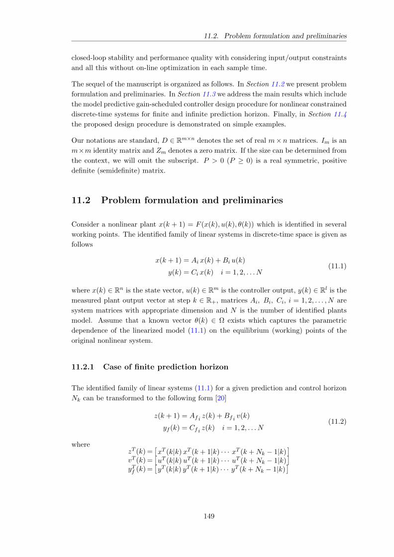
11.2. Problem formulation and preliminaries
closed-loop stability and performance quality with considering input/output constraints
and all this without on-line optimization in each sample time.
The sequel of the manuscript is organized as follows. In Section 11.2 we present problem
formulation and preliminaries. In Section 11.3 we address the main results which include
the model predictive gain-scheduled controller design procedure for nonlinear constrained
discrete-time systems for finite and infinite prediction horizon. Finally, in Section 11.4
the proposed design procedure is demonstrated on simple examples.
Our notations are standard, D ∈ Rm×n denotes the set of real m×n matrices. Im is an
m×m identity matrix and Zm denotes a zero matrix. If the size can be determined from
the context, we will omit the subscript. P > 0 (P ≥ 0) is a real symmetric, positive
definite (semidefinite) matrix.
11.2 Problem formulation and preliminaries
Consider a nonlinear plant x(k + 1) = F (x(k), u(k), θ(k)) which is identified in several
working points. The identified family of linear systems in discrete-time space is given as
follows
x(k + 1) = Ai x(k) +Bi u(k)
y(k) = Ci x(k) i = 1, 2, . . . N(11.1)
where x(k) ∈ Rn is the state vector, u(k) ∈ Rm is the controller output, y(k) ∈ Rl is the
measured plant output vector at step k ∈ R+, matrices Ai, Bi, Ci, i = 1, 2, . . . , N are
system matrices with appropriate dimension and N is the number of identified plants
model. Assume that a known vector θ(k) ∈ Ω exists which captures the parametric
dependence of the linearized model (11.1) on the equilibrium (working) points of the
original nonlinear system.
11.2.1 Case of finite prediction horizon
The identified family of linear systems (11.1) for a given prediction and control horizon
Nk can be transformed to the following form [20]
z(k + 1) = Af i z(k) +Bf i v(k)
yf (k) = Cf i z(k) i = 1, 2, . . . N(11.2)
wherezT (k) =
[xT (k|k) xT (k + 1|k) · · · xT (k +Nk − 1|k)
]vT (k) =
[uT (k|k) uT (k + 1|k) · · · uT (k +Nk − 1|k)
]yTf (k) =
[yT (k|k) yT (k + 1|k) · · · yT (k +Nk − 1|k)
]
149
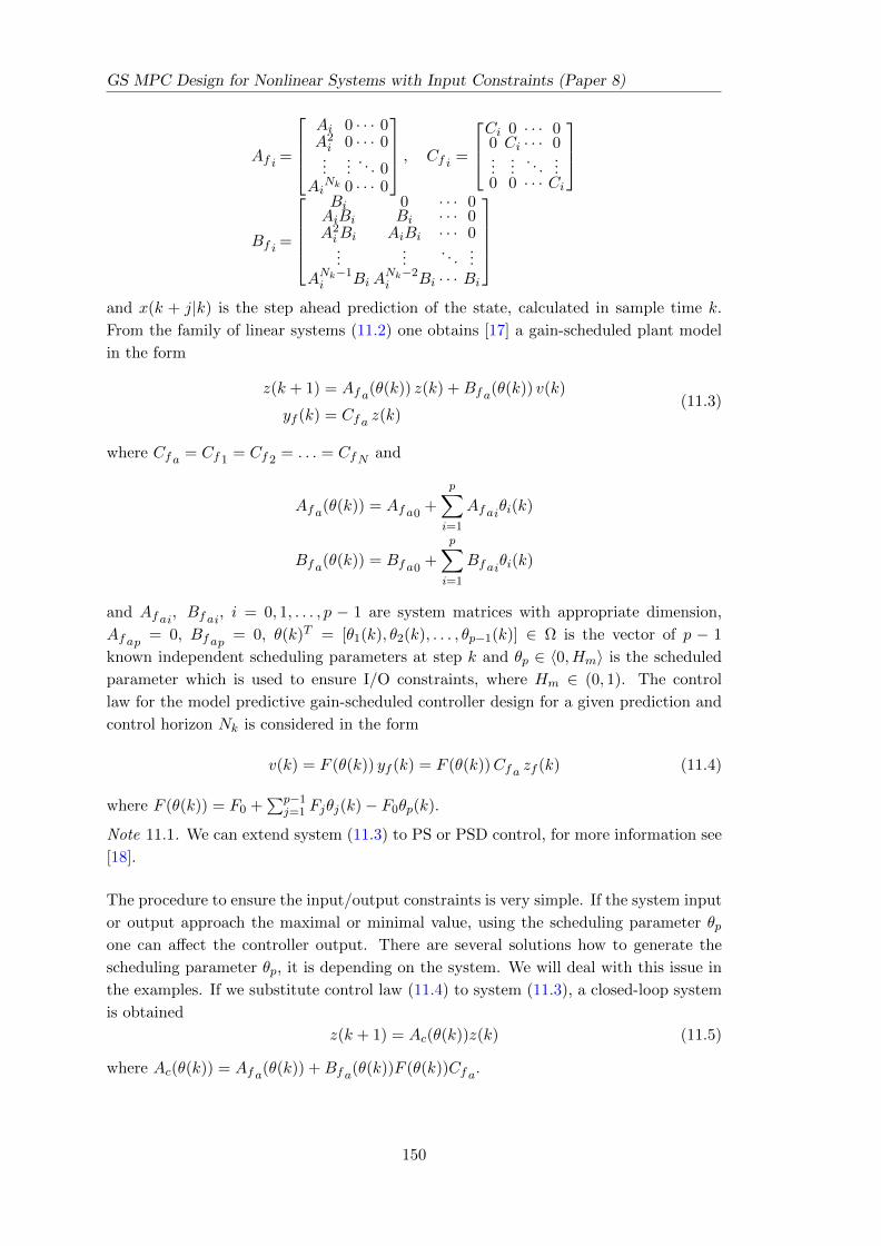
GS MPC Design for Nonlinear Systems with Input Constraints (Paper 8)
Af i =
Ai 0 · · · 0A2i 0 · · · 0
......
. . . 0Ai
Nk 0 · · · 0
, Cf i =
Ci 0 · · · 00 Ci · · · 0...
.... . .
...0 0 · · · Ci
Bf i =
Bi 0 · · · 0AiBi Bi · · · 0A2iBi AiBi · · · 0...
.... . .
...ANk−1i Bi A
Nk−2i Bi · · · Bi
and x(k + j|k) is the step ahead prediction of the state, calculated in sample time k.
From the family of linear systems (11.2) one obtains [17] a gain-scheduled plant model
in the form
z(k + 1) = Af a(θ(k)) z(k) +Bf a(θ(k)) v(k)
yf (k) = Cf a z(k)(11.3)
where Cf a = Cf 1 = Cf 2 = . . . = CfN and
Af a(θ(k)) = Af a0+
p∑i=1
Af aiθi(k)
Bf a(θ(k)) = Bf a0+
p∑i=1
Bf aiθi(k)
and Af ai, Bf ai, i = 0, 1, . . . , p − 1 are system matrices with appropriate dimension,
Af ap = 0, Bf ap = 0, θ(k)T = [θ1(k), θ2(k), . . . , θp−1(k)] ∈ Ω is the vector of p − 1
known independent scheduling parameters at step k and θp ∈ 〈0, Hm〉 is the scheduled
parameter which is used to ensure I/O constraints, where Hm ∈ (0, 1). The control
law for the model predictive gain-scheduled controller design for a given prediction and
control horizon Nk is considered in the form
v(k) = F (θ(k)) yf (k) = F (θ(k))Cf a zf (k) (11.4)
where F (θ(k)) = F0 +∑p−1
j=1 Fjθj(k)− F0θp(k).
Note 11.1. We can extend system (11.3) to PS or PSD control, for more information see
[18].
The procedure to ensure the input/output constraints is very simple. If the system input
or output approach the maximal or minimal value, using the scheduling parameter θpone can affect the controller output. There are several solutions how to generate the
scheduling parameter θp, it is depending on the system. We will deal with this issue in
the examples. If we substitute control law (11.4) to system (11.3), a closed-loop system
is obtained
z(k + 1) = Ac(θ(k))z(k) (11.5)
where Ac(θ(k)) = Af a(θ(k)) +Bf a(θ(k))F (θ(k))Cf a.
150
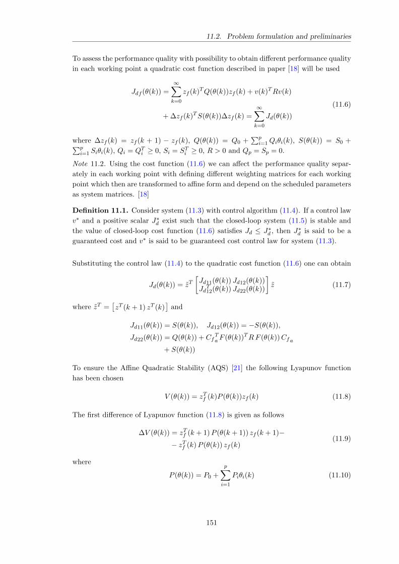
11.2. Problem formulation and preliminaries
To assess the performance quality with possibility to obtain different performance quality
in each working point a quadratic cost function described in paper [18] will be used
Jdf (θ(k)) =
∞∑k=0
zf (k)TQ(θ(k))zf (k) + v(k)TRv(k)
+ ∆zf (k)TS(θ(k))∆zf (k) =
∞∑k=0
Jd(θ(k))
(11.6)
where ∆zf (k) = zf (k + 1) − zf (k), Q(θ(k)) = Q0 +∑p
i=1Qiθi(k), S(θ(k)) = S0 +∑pi=1 Siθi(k), Qi = QTi ≥ 0, Si = STi ≥ 0, R > 0 and Qp = Sp = 0.
Note 11.2. Using the cost function (11.6) we can affect the performance quality separ-
ately in each working point with defining different weighting matrices for each working
point which then are transformed to affine form and depend on the scheduled parameters
as system matrices. [18]
Definition 11.1. Consider system (11.3) with control algorithm (11.4). If a control law
v∗ and a positive scalar J∗d exist such that the closed-loop system (11.5) is stable and
the value of closed-loop cost function (11.6) satisfies Jd ≤ J∗d , then J∗d is said to be a
guaranteed cost and v∗ is said to be guaranteed cost control law for system (11.3).
Substituting the control law (11.4) to the quadratic cost function (11.6) one can obtain
Jd(θ(k)) = zT[Jd11(θ(k)) Jd12(θ(k))JdT12(θ(k)) Jd22(θ(k))
]z (11.7)
where zT =[zT (k + 1) zT (k)
]and
Jd11(θ(k)) = S(θ(k)), Jd12(θ(k)) = −S(θ(k)),
Jd22(θ(k)) = Q(θ(k)) + CfTa F (θ(k))TRF (θ(k))Cf a
+ S(θ(k))
To ensure the Affine Quadratic Stability (AQS) [21] the following Lyapunov function
has been chosen
V (θ(k)) = zTf (k)P (θ(k))zf (k) (11.8)
The first difference of Lyapunov function (11.8) is given as follows
∆V (θ(k)) = zTf (k + 1)P (θ(k + 1)) zf (k + 1)−− zTf (k)P (θ(k)) zf (k)
(11.9)
where
P (θ(k)) = P0 +
p∑i=1
Piθi(k) (11.10)
151
GS MPC Design for Nonlinear Systems with Input Constraints (Paper 8)
On substituting θ(k+ 1) = θ(k) + ∆θ(k) to P (θ(k+ 1)) one obtains the following result
P (θ(k + 1)) = P0 +
p∑i=1
Piθi(k) +
p∑i=1
Pi∆θi(k) (11.11)
where if assuming that Pi > 0, ∆θi ∈ 〈∆θi,∆θi〉 ∈ Ωt, i = 0, 1, . . . p and max |∆θi| < ρi,
one can write
P (θ(k + 1)) ≤ P0 +
p∑i=1
Piθi(k) + Pρ = Pρ(θ(k)) (11.12)
where Pρ =∑p
i=1 Piρi. The first difference of the Lyapunov function (11.9) using the
free matrix weighting approach [17] is in the form
∆V (θ(k)) = zT[V11(θ(k)) V12(θ(k))V T
12(θ(k)) V22(θ(k))
]z (11.13)
whereV11(θ(k)) =Pρ(θ(k)) +N1 +NT
1V12(θ(k)) =NT
2 −N1Ac(θ(k))V22(θ(k)) =−P (θ(k))−N2Ac(θ(k))−ATc (θ(k))NT
2
where N1, N2 ∈ Rn×n are auxiliary matrices.
Definition 11.2. [21] The linear closed-loop system (11.5) for θ(k) ∈ Ω and ∆θ(k) ∈ Ωt
is affinely quadratically stable if and only if p + 1 symmetric matrices P0, P1, . . . , Ppexist such that P (θ(k)) (11.10), Pρ(θ(k)) (11.12) are positive defined and for the first
difference of the Lyapunov function (11.13) along the trajectory of closed-loop system
(11.5) it holds
∆V (θ(k)) < 0 (11.14)
From LQ theory we can introduce the well known results:
Lemma 11.1. Consider the closed-loop system (11.5). Closed-loop system (11.5) is
affinely quadratically stable with guaranteed cost if and only if the following inequality
holds
Be(θ(k)) = minu∆V (θ(k)) + Jd(θ(k)) ≤ 0 (11.15)
for all θ(k) ∈ Ω. For proof see [22].
11.2.2 Case of infinite prediction horizon
The system described by (11.3) for the case of Nk = 0 can be transformed to the gain-
scheduled plant model
x(k + 1) = A(θ(k))x(k) +B(θ(k))u(k)
y(k) = C x(k)(11.16)
152
11.2. Problem formulation and preliminaries
where A(θ(k)) = A0 +∑p
i=1Aiθi(k), B(θ(k)) = B0 +∑p
i=1Biθi(k), Ap = 0 and Bp = 0.
For the case Nk →∞ and S = 0 the cost function (11.6) can be rewritten as
J =
∞∑k=0
J(k) =
∞∑k=0
∞∑j=0
xT (k + j)qjx(k + j)
+uT (k + j)rju(k + j)
)=∞∑k=0
∞∑j=0
J(k)
(11.17)
where qj ∈ Rn×n, rj ∈ Rm×m are positive definite matrices. The control law for the
model predictive gain-scheduled controller design for the infinite prediction horizon is
considered in the form
u(k) = F (θ(k)) y(k) = F (θ(k))C x(k) (11.18)
where F (θ(k)) = F0 +∑p−1
j=1 Fjθj(k) − F0θp(k). To guarantee the stability and per-
formance of the closed-loop gain-scheduled system, due to Lemma 11.1 it is sufficient to
ensure
Be(θ(k)) = ∆V (x(k + j), θ(k)) + J(k) ≤ 0 (11.19)
where ∆V (x(k + j), θ(k)) = V (x(k + j + 1), θ(k) + ∆θ(k)) − V (x(k), θ(k)) is the first
difference of the Lyapunov function for j horizon prediction. Summing (11.19) from
j = 0 to j →∞, the upper bound on J(k) is obtained
J(k) ≤ V (x(k), θ(k)) (11.20)
On the basis of (11.20) the following gain-scheduled MPC design procedure is given
minF (θ(k))
V (x(k), θ(k)) (11.21)
with constraints to system model (11.16), stability model and performance (11.19) and
other constraints. Assume that the Lyapunov function is in the form V (x(k), θ(k)) =
xT (k)P (θ(k))x(k), where P (θ) = P0 +∑p
i=1 Piθi(k). Due to (11.21), the predicted
control design procedure can be modified as
minF (θ(k))
xT (k)P (θ(k))x(k) ≤ xT (k)x(k)γ (11.22)
which leads to the inequality
P (θ(k)) ≤ minF (θ(k))
γI (11.23)
In the paper [23] inequality (11.22) is in the form
min xT (k)P (θ(k))x(k) ≤ γ (11.24)
which needs to know the state vector x(k) and on-line optimization of (11.24) at every
sample time.
153
GS MPC Design for Nonlinear Systems with Input Constraints (Paper 8)
The stability of the closed-loop system is guaranteed if
Be = ∆V (x(k), θ(k)) + αV (x(k), θ(k)) ≤ 0 (11.25)
where α ∈ 〈0, 1) is a coefficient with an influence on the closed-loop system performance.
If we substitute the Lyapunov function and its first difference to (11.25), we can obtain
Be(θ(k)) = xTW (θ(k)) x ≤ 0 (11.26)
where xT =[xT (k + 1) xT (k)
], β = 1− α and
W (θ(k)) =
[W11(θ(k)) W12(θ(k))W12(θ(k))T W22(θ(k))
]W11(θ(k)) =NT
1 +N1 + Pρ(θ(k))W12(θ(k)) =−NT
1 Ac(θ(k)) +N2
W22(θ(k)) =−N2Ac(θ(k))−ATc (θ(k))N2 − P (θ(k))(β)
11.3 Main results
In this section the discrete predictive gain-scheduled controller design procedure is
presented which guarantees the affine quadratic stability and guaranteed cost for
θ(k) ∈ Ω with pre-defined maximal rate of change of the scheduled parameters ρ. The
main result of this section – the discrete model predictive gain-scheduled controller design
procedure – relies on the concept of multi-convexity, that is convexity along each dir-
ection θi(k), i = 1, 2, . . . , p of the parameter space. The implications of multiconvexity
for scalar quadratic functions are given in the next lemma [21].
Lemma 11.2. Consider a scalar quadratic function of α ∈ Rp.
f (α) = a0 +
p∑i=1
aiαi +
p∑i=1
p∑j>i
bijαiαj +
p∑i=1
ciα2i (11.27)
and assume that f (α1, . . . , αp) is multi-convex, that is ∂2f(α)∂α2
i= 2ci ≥ 0 for i =
1, 2, . . . , p. Then f(α) is negative for all α ∈ Ω and α ∈ Ωt if and only if it takes
negative values at the corners of α.
11.3.1 Finite prediction horizon
Using Lemmas 11.1 and 11.2 the following theorem is obtained for discrete model pre-
dictive gain-scheduled controller design for finite horizon.
Theorem 11.1. Closed-loop system (11.5) is affinely quadratically stable if p+1 symmet-
ric matrices P0, P1, . . . , Pp exist such that P (θ(k)) (11.10), Pρ(θ(k)) (11.12) are positive
definite for all θ(k) ∈ Ω, with pre-defined ρi, matrices N1, N2, Qi, R, Si, i = 1, 2, . . . p
154
11.3. Main results
and gain-scheduled matrices F (θ(k)) satisfying
M(θ(k)) < 0; θ(k) ∈ Ω
Mii ≥ 0; i = 1, 2, . . . , p(11.28)
where (at sample time k)
M(θ) =M0 +∑p
i=1Miθi +∑p
i=1
∑p−1j>i Mijθiθj +
∑pi=1Miiθ
2i
M0 =
[M110 M120M12
T0 M220
], Mi =
[M11i M12iM12
Ti M22i
]Mij =
[M11ijM12ij
M12TijM22ij
],M110 = P0 +N1 +NT
1 + S0 + Pρ
M11i =Pi, M11ij = 0, M11ii = 0M120 =N2 −NT
1 (Af a0+Bf a0
F0Cf a)− S0
M12i =−NT1 (Af ai +Bf aiF0Cf a +Bf a0
FiCf a)− SiM12ij =−NT
1 (Bf aiFj +Bf ajFi)Cf aM12ii =−NT
1 Bf aiFiCf aM220 =Q0 + S0 − P0 −NT
2 (Af a0+Bf a0
F0Cf a)
−(Af a0+Bf a0
F0Cf a)TN2 + Cf
Ta F
T0 RF0Cf a
M22i =−Pi −NT2 (Af ai +Bf aiF0Cf a +Bf a0
FiCf a)
−(Af ai +Bf aiF0Cf a +Bf a0FiCf a)
TN2
+CfTa (F T0 RFi + F Ti RF0)Cf a +Qi + Si
M22ij =−NT2 (Bf aiFj +Bf ajFi)Cf a − Cf
Ta (Bf aiFj
+Bf ajFi)TN2 + Cf
Ta (F Ti RFj + F Tj RFi)Cf a
M22ii =−NT2 Bf aiFiCf a − (Bf aiFiCf a)
TN2
+CfTa F
Ti RFiCf a
Proof. The proof of the Theorem 11.1 is clear from the previous derivations. Here,
the proof is repeated only in basic steps. The proof is based on the Lemmas 11.1 and
11.2. When substituting the first difference of the Lyapunov function (11.13) and the
quadratic cost function (11.7) to the Bellman-Lyapunov function (11.15), after some
manipulation, using Lemma 11.2 we obtain (11.28) which proofs the Theorem 11.1.
11.3.2 Infinite prediction horizon
Using inequalities (11.23), (11.26) and Lemma 11.2 the following theorem is obtained
for discrete model predictive gain-scheduled controller design for infinite horizon.
Theorem 11.2. Closed-loop system is affinely quadratically stable if there exist p + 1
symmetric matrices P0, P1, . . . , Pp such that P (θ(k)) (11.10), Pρ(θ(k)) (11.12) are pos-
itive definite for all θ(k) ∈ Ω, with pre-defined ρi, matrices N1, N2, and gain-scheduled
matrices F (θ(k)) satisfying
W (θ(k)) < 0; θ(k) ∈ Ω
Wii ≥ 0; i = 1, 2, . . . , p
P (θ(k)) ≤ minF (θ(k))
γ
(11.29)
155
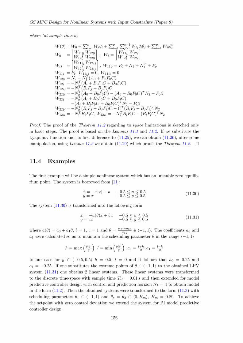
GS MPC Design for Nonlinear Systems with Input Constraints (Paper 8)
where (at sample time k)
W (θ) =W0 +∑p
i=1Wiθi +∑p
i=1
∑p−1j>i Wijθiθj +
∑pi=1Wiiθ
2i
W0 =
[W110 W120W12
T0 W220
], Wi =
[W11i W12iW12
Ti W22i
]Wij =
[W11ijW12ij
W12TijW22ij
], W110 = P0 +N1 +NT
1 + Pρ
W11i =Pi, W11ij = 0, W11ii = 0W120 =N2 −NT
1 (A0 +B0F0C)W12i =−NT
1 (Ai +BiF0C +B0FiC),W12ij =−NT
1 (BiFj +BjFi)CW220 =−NT
2 (A0 +B0F0C)− (A0 +B0F0C)TN2 − P0βW22i =−NT
2 (Ai +BiF0C +B0FiC)−(Ai +BiF0C +B0FiC)TN2 − Piβ
W22ij =−NT2 (BiFj +BjFi)C − CT (BiFj +BjFi)
TN2
W12ii =−NT1 BiFiC, W22ii = −NT
2 BiFiC − (BiFiC)TN2
Proof. The proof of the Theorem 11.2 regarding to space limitations is sketched only
in basic steps. The proof is based on the Lemmas 11.1 and 11.2. If we substitute the
Lyapunov function and its first difference to (11.25), we can obtain (11.26), after some
manipulation, using Lemma 11.2 we obtain (11.29) which proofs the Theorem 11.2.
11.4 Examples
The first example will be a simple nonlinear system which has an unstable zero equilib-
rium point. The system is borrowed from [11]:
x = −x|x|+ u −0.5 ≤ u ≤ 0.5y = x −0.5 ≤ y ≤ 0.5 (11.30)
The system (11.30) is transformed into the following form
x = −a(θ)x+ bu −0.5 ≤ u ≤ 0.5y = cx −0.5 ≤ y ≤ 0.5 (11.31)
where a(θ) = a0 + a1θ, b = 1, c = 1 and θ = y|y|−a0ya1y
∈ 〈−1, 1〉. The coefficients a0 and
a1 were calculated so as to maintain the scheduling parameter θ in the range 〈−1, 1〉
h = max(y|y|y
); l = min
(y|y|y
); a0 = l+h
2 ; a1 = l−h2
In our case for y ∈ 〈−0.5, 0.5〉 h = 0.5, l = 0 and it follows that a0 = 0.25 and
a1 = −0.25. If one substitutes the extreme points of θ ∈ 〈−1, 1〉 to the obtained LPV
system (11.31) one obtains 2 linear systems. These linear systems were transformed
to the discrete time-space with sample time Tst = 0.01 s and then extended for model
predictive controller design with control and prediction horizon Nk = 4 to obtain model
in the form (11.2). Then the obtained systems were transformed to the form (11.3) with
scheduling parameters θ1 ∈ 〈−1, 1〉 and θp = θ2 ∈ 〈0, Hm〉, Hm = 0.89. To achieve
the setpoint with zero control deviation we extend the system for PI model predictive
controller design.
156
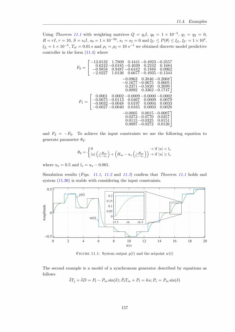
11.4. Examples
Using Theorem 11.1 with weighting matrices Q = qiI, q0 = 1 × 10⁻⁵, q1 = q2 = 0,
R = rI, r = 10, S = siI, s0 = 1× 10−50, s1 = s2 = 0 and ξU ≤ P (θ) ≤ ξL, ξU = 1× 10⁴,
ξL = 1× 10⁻⁵, Tst = 0.01 s and ρ1 = ρ2 = 10 s−1 we obtained discrete model predictive
controller in the form (11.4) where
F0 =
−13.0132 1.7809 0.4441−0.4923−0.35570.6242−0.0185−0.4039 0.2242 0.1684−0.9858 0.9487−0.6442 0.1888 0.0962−2.0227 1.0136 0.6677−0.4935−0.1344
−0.0963 0.3846−0.2068−0.1677−0.0675 0.0605
0.2371−0.5820 0.26990.0092 0.3362−0.1747
F1 =
0.0001 0.0002−0.0009−0.0000−0.0002−0.0075−0.0113 0.0467 0.0009 0.0079−0.0032−0.0048 0.0197 0.0004 0.0033−0.0027−0.0040 0.0165 0.0003 0.0028
−0.0005 0.0015−0.00070.0273−0.0770 0.03570.0115−0.0325 0.01510.0097−0.0272 0.0126
and F2 = −F0. To achieve the input constraints we use the following equation to
generate parameter θ2:
θ2 =
0 → if |u| < ls
|u|(
−Hm
ls−us
)+(Hm − us
(−Hm
ls−us
))→ if |u| ≥ ls
where us = 0.5 and ls = us − 0.001.
Simulation results (Figs. 11.1, 11.2 and 11.3) confirm that Theorem 11.1 holds and
system (11.30) is stable with considering the input constraints.
Figure 11.1: System output y(t) and the setpoint w(t)
The second example is a model of a synchronous generator described by equations as
follows
δTj + δD = Pt − Pm sin(δ); PtTm + Pt = ku;Pe = Pm sin(δ)
157
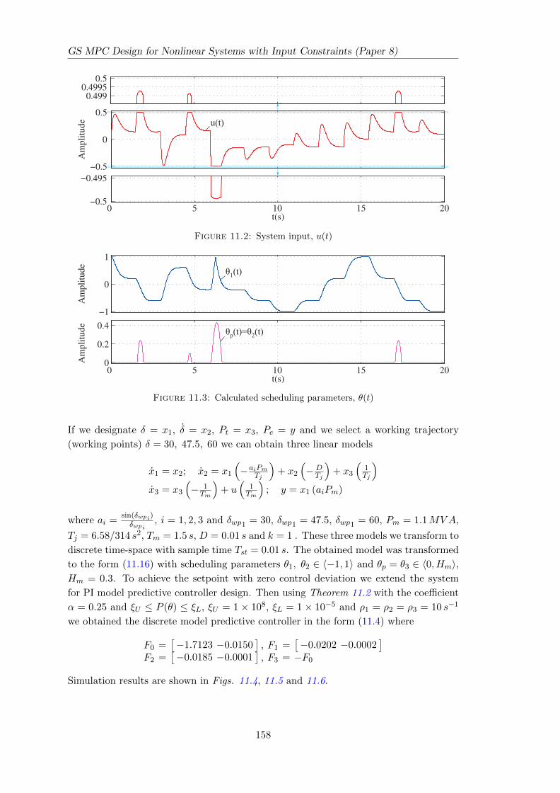
GS MPC Design for Nonlinear Systems with Input Constraints (Paper 8)
Figure 11.2: System input, u(t)
Figure 11.3: Calculated scheduling parameters, θ(t)
If we designate δ = x1, δ = x2, Pt = x3, Pe = y and we select a working trajectory
(working points) δ = 30, 47.5, 60 we can obtain three linear models
x1 = x2; x2 = x1
(−aiPm
Tj
)+ x2
(−DTj
)+ x3
(1Tj
)x3 = x3
(− 1Tm
)+ u
(1Tm
); y = x1 (aiPm)
where ai =sin(δwpi)δwpi
, i = 1, 2, 3 and δwp1 = 30, δwp1 = 47.5, δwp1 = 60, Pm = 1.1MVA,
Tj = 6.58/314 s2, Tm = 1.5 s, D = 0.01 s and k = 1 . These three models we transform to
discrete time-space with sample time Tst = 0.01 s. The obtained model was transformed
to the form (11.16) with scheduling parameters θ1, θ2 ∈ 〈−1, 1〉 and θp = θ3 ∈ 〈0, Hm〉,Hm = 0.3. To achieve the setpoint with zero control deviation we extend the system
for PI model predictive controller design. Then using Theorem 11.2 with the coefficient
α = 0.25 and ξU ≤ P (θ) ≤ ξL, ξU = 1× 10⁸, ξL = 1× 10⁻⁵ and ρ1 = ρ2 = ρ3 = 10 s−1
we obtained the discrete model predictive controller in the form (11.4) where
F0 =[−1.7123 −0.0150
], F1 =
[−0.0202 −0.0002
]F2 =
[−0.0185 −0.0001
], F3 = −F0
Simulation results are shown in Figs. 11.4, 11.5 and 11.6.
158
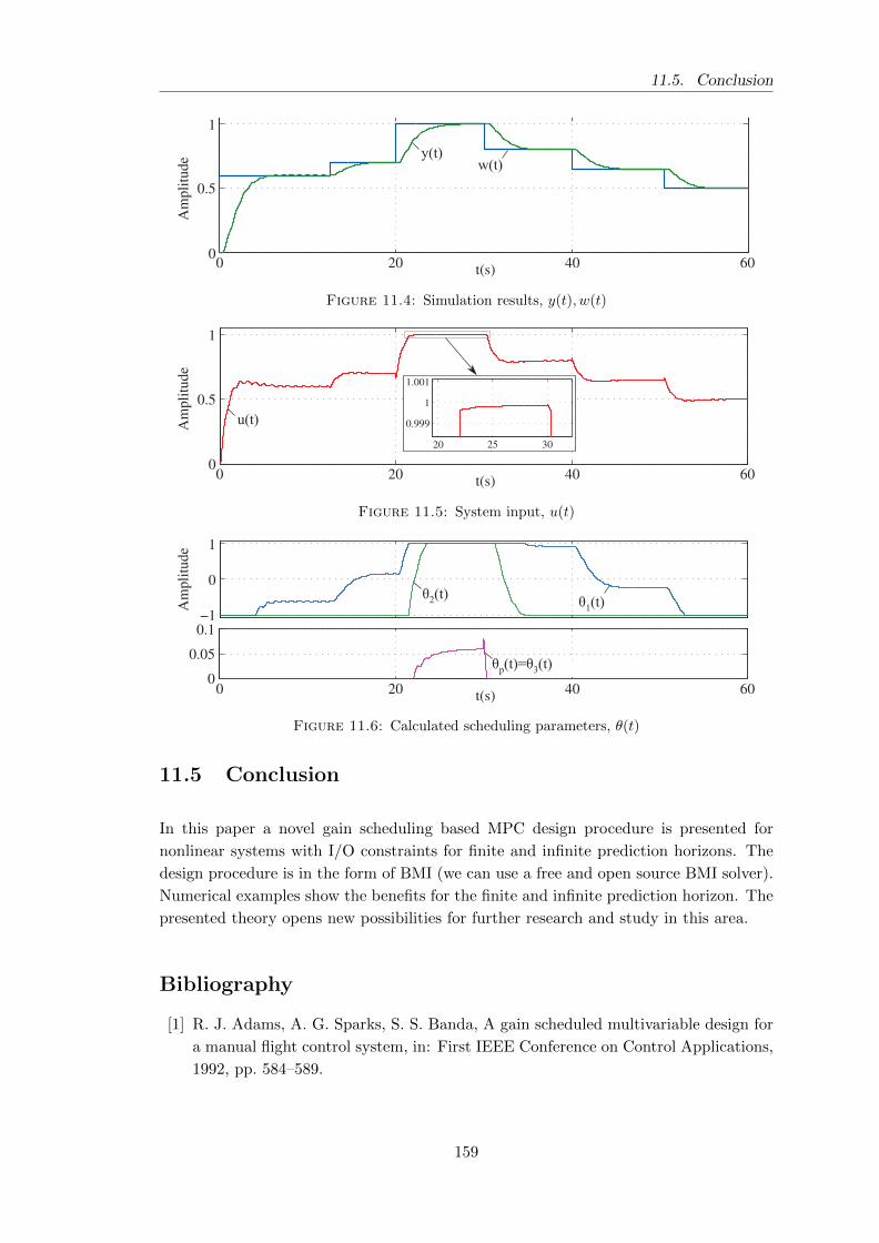
11.5. Conclusion
Figure 11.4: Simulation results, y(t), w(t)
Figure 11.5: System input, u(t)
Figure 11.6: Calculated scheduling parameters, θ(t)
11.5 Conclusion
In this paper a novel gain scheduling based MPC design procedure is presented for
nonlinear systems with I/O constraints for finite and infinite prediction horizons. The
design procedure is in the form of BMI (we can use a free and open source BMI solver).
Numerical examples show the benefits for the finite and infinite prediction horizon. The
presented theory opens new possibilities for further research and study in this area.
Bibliography
[1] R. J. Adams, A. G. Sparks, S. S. Banda, A gain scheduled multivariable design for
a manual flight control system, in: First IEEE Conference on Control Applications,
1992, pp. 584–589.
159
GS MPC Design for Nonlinear Systems with Input Constraints (Paper 8)
[2] R. A. Nichols, R. T. Reichert, W. J. Rugh, Gain Scheduling for h∞ Controllers:
A Flight Control Example, IEEE Transactions on Control Systems Technology 1
(1993) 69–79.
[3] R. Hyde, K. Glover, The application of scheduled h∞ controllers to a VSTOL
aircraft, IEEE Transactions on Automatic Control 38 (7) (1993) 1021–1039.
[4] J. S. Shamma, Control of Linear Parameter Varying Systems with Applications,
Springer, 2012, Ch. An overview of LPV systems, pp. 3–26.
[5] F. Forni, S. Galeani, Gain-scheduled, model-based anti-windup for LPV systems,
Automatica 46 (1) (2010) 222 – 225.
[6] F. Forni, S. Galeani, Model based, gain-scheduled anti-windup control for LPV
systems, in: 46th IEEE Conference on Decision and Control, 2007, 2007, pp. 1174–
1179.
[7] S. J. Qin, T. A. Badgwell, A survey of industrial model predictive control technology,
Control Engineering Practice 11 (7) (2003) 733 – 764.
[8] D. Q. Mayne, J. B. Rawlings, C. V. Rao, P. O. M. Scokaert, Constrained model
predictive control: Stability and optimality, Automatica 36 (6) (2000) 789 – 814.
[9] L. Magni, R. Scattolini, Stabilizing model predictive control of nonlinear continuous
time systems, Annual Reviews in Control 28 (1) (2004) 1 – 11.
[10] S. M. Lee, J. H. Park, Output feedback model predictive control for LPV systems
using parameter-dependent Lyapunov function, Applied Mathematics and Compu-
tation 190 (1) (2007) 671 – 676.
[11] M. F. Hassan, M. Zribi, An observer-based controller for nonlinear systems: A gain
scheduling approach, Applied Mathematics and Computation 237 (0) (2014) 695 –
711.
[12] Z. Wan, M. V. Kothare, A framework for design of scheduled output feedback model
predictive control, Journal of Process Control 18 (3–4) (2008) 391 – 398, festschrift
honouring Professor Dale Seborg.
[13] A. Abdullah, M. Zribi, Model reference control of LPV systems, Journal of the
Franklin Institute 346 (9) (2009) 854 – 871.
[14] J.-H. Park, T.-H. Kim, T. Sugie, Output feedback model predictive control for LPV
systems based on quasi-min–max algorithm, Automatica 47 (9) (2011) 2052 – 2058.
[15] Z. Wan, M. V. Kothare, Robust output feedback model predictive control using
off-line linear matrix inequalities, Journal of Process Control 12 (7) (2002) 763 –
774.
[16] Y.-B. Zhao, J. Kim, G.-P. Liu, Offline model predictive control-based gain schedul-
ing for networked control systems [brief paper], Control Theory Applications, IET
6 (16) (2012) 2585–2591.
160
Bibliography
[17] V. Vesely, A. Ilka, Gain-scheduled PID controller design, Journal of Process Control
23 (8) (2013) 1141–1148.
[18] A. Ilka, V. Vesely, Discrete gain-scheduled controller design: Variable weighting
approach, in: 15th International Carpathian Control Conference (ICCC), 2014,
2014, pp. 186–191.
[19] V. Vesely, A. Ilka, PID robust gain-scheduled controller design, in: 2014 European
Control Conference (ECC), 2014, pp. 2756–2761.
[20] D. Vozak, V. Vesely, Robust Model Predictive Controller Design, in: Preprints of
the 19th IFAC World Congress, The International Federation of Automatic Control,
Cape Town, South Africa, 2014, pp. 7443–7448.
[21] P. Gahinet, P. Apkarian, M. Chilali, Affine parameter-dependent Lyapunov func-
tions and real parametric uncertainty, IEEE Transactions on Automatic Control
41 (3) (1996) 436–442.
[22] V. M. Kuncevic, M. M. Lycak, Control systems design using Lyapunov function
approach, Vol. in Russian, Nauka, Moskau, 1977.
[23] M. V. Kothare, V. Balakrishnan, M. Morari, Robust constrained model predictive
control using linear matrix inequalities, Automatica 32 (10) (1996) 1361 – 1379.
161

12
Unified Robust Gain-Scheduled
and Switched Controller Design
for Linear Continuous-Time Systems
(Paper 9)
Abstract
In this paper we study the problem how to obtain a new unified procedure to design a
robust gain-scheduled and switched controller for continuous-time systems described by
a novel robust plant model using the parameter dependent quadratic stability (PDQS)
approach. In the proposed design procedure with output feedback a novel quadratic
cost function is proposed which allows to obtain different performance dependence on
the working points. Finally a numerical example is investigated.
Keywords: Gain-scheduled controller, switched system, robust controller, output feed-
back, parameter dependent quadratic stability.
12.1 Introduction
The topic of robust hybrid systems has attracted considerable attention in the past
decades. Wherever continuous and discrete dynamics interact, a hybrid system arises.
The main motivation for studying hybrid systems comes from the two facts:
• hybrid systems have numerous applications in the real world, and
• in real control, there are dynamical systems that cannot be stabilized by any
continuous static (dynamic) output state controller but a stabilizing hybrid control
scheme can be found.
163
Unified Robust Gain-Scheduled and Switched Controller Design (Paper 9)
There are several approaches to model hybrid systems [1], [2]. In the references they
consider a discrete even system and continuous dynamics modeled by differential or
difference equations. Such models are used to formulate general stability conditions
for hybrid systems. In this paper, we consider the class of hybrid systems known as
switched systems [3]. There are at last two approaches for stability analysis and control-
ler synthesis of switched systems. The quadratic stability approach with the common
Lyapunov function gives stability of closed-loop switched systems under an arbitrary
switching law and a multiple Lyapunov function which is less conservative. The survey
of the present status of switched systems can be consulted in the excellent paper and
work of [4], [1] and [5]. A huge number of references can be found in the switched con-
trol of linear discrete-time invariant systems but in the field of linear continuous-time
invariant systems the number of references is rather small. The representatives are the
following references [6], [7], [8], [9], [10].
In real applications a controller must accommodate a plant with changing dynamics.
Therefore, controllers based on these models have to be robust in the presence of plant
model uncertainty. In a practical situation one could use the gain scheduling approach
which involves scheduling in a family of local controllers in response to the changing
plant dynamics. The proposed family of local controllers is implemented using the gain
scheduling approach. The classical gain scheduling design procedure typically involves
the following steps [11]
• The equilibrium operating points are parameterized by an appropriate quantity
θT = [θ1, . . . , θp] which may be involve to the plant input and output.
• The plant dynamics is approximated, locally to a specific equilibrium operating
point at which one obtains different values of θ.
• For a given controller structure with a value of θ a linear time-invariant controller
is designed. It should be noted that θ is assumed to be constant when designing
this controller.
• Repeat steps 2 and 3 for a family of operating points. Family of controllers are
parameterized by θ.
A survey of gain-scheduled controller design can be found in [11], [12] and [13] using
linear controller design techniques. In our paper, using a new uncertain plant model, a
unified approach to design a robust gain-scheduled and robust switched controller with
an arbitrarily switching law [1] is developed for continuous-time linear systems. Using
multiple parameter dependent Lyapunov function the novel robust gain-scheduled and
switched controller design procedure is obtained in the form of BMI. In the proposed
design procedure there is no need to use the approach of ”dwell time” [6], [7] for switched
controller design with arbitrary switching. The ”dwell time” markedly complicates the
robust switched controller design procedure and makes the obtained results conservative.
The advantages of the proposed method are as follows:
164
12.2. Problem formulation and preliminaries
• a unified approach to robust gain-scheduled and robust switched controller design
with arbitrary switching for linear continuous-time system has been developed,
• in the method proposed in the paper for the case of switched controller design with
arbitrary switching there is no need to use the approach of ”dwell-time”,
• the switched controller designer can take into account the non-ideal switching, that
is switching a variable with a rate of switching less than infinite, which open the
new possibility for the controller designer,
• different performance could be prescribed by the proposed new cost function for
all plant modes.
Organization of the paper is following. Section 12.2 includes problem formulation of the
robust gain-scheduled or switched controller design and some preliminaries are given.
In Section 12.3 sufficient stability conditions to design the robust gain-scheduled or
switched controller in the form of BMI are given. In Section 12.4 the obtained results
are illustrated on real examples.
12.2 Problem formulation and preliminaries
The class of LPV uncertain continuous-time systems considered in the paper can be
represented by the following model
x(t) = A(ξ, θ)x(t) +B(ξ, θ)u(t)y(t) = Cx(t)
(12.1)
where x(t) ∈ Rn is the state vector, u(t) ∈ Rm is the control vector, y(t) ∈ Rl is the
output vector of the system to be controlled. Time varying scheduling parameter vector
θT = [θ1, . . . , θp] is assumed to belong to a hyper rectangle:
• Gain-Scheduled Controller
θi ∈ 〈θi, θi〉, i = 1, 2, . . . , p, θi = −θi, θi ∈ 〈θi, θi〉 (12.2)
• Switched Controller Design
θi ∈ 〈0, 1〉, i = 1, 2, . . . , p,
p∑i=1
θi = 1,
p∑i=1
θi = 0 (12.3)
θi ∈ 〈θi, θi〉
where θi, i = 1, 2, . . . , p is a switching variable with an arbitrary switching al-
gorithm and p is the number of switching plant modes. Observation of (12.1)
implies that for an arbitrary switching algorithm the number of active switching
plant modes generates the value of switching variable θi, i = 1, 2, . . . , p to determ-
ine which controller will be active.
165
Unified Robust Gain-Scheduled and Switched Controller Design (Paper 9)
• Assume that for both cases hold θ ∈ Ω, θ ∈ Ωt
There are two possibilities for switching parameters θi, i = 1, 2, . . . , p
1. the rates of change of the switching parameters are infinite, ideal switching case,
in this case the quadratic stability with respect to parameter θ can be used or
2. the rates of change of switching parameters θi are finite, non-ideal case, in this
case the PDQS is recommended to use.
Affine dependence on the scheduling (switching) parameter vector is assumed as follows
A(ξ, θ) = A0(ξ) +
p∑i=1
Ai(ξ)θi ∈ Rn×n
B(ξ, θ) = B0(ξ) +
p∑i=1
Bi(ξ)θi ∈ Rn×m(12.4)
where Ai(ξ), Bi(ξ), i = 0, 1, . . . , p belong to a convex polytope box with N vertices that
can be formally defined as
Ω =
Ai(ξ), Bi(ξ) =
N∑j=1
(Aij , Bij)ξj , i = 0, 1, . . . , p,
N∑j=1
ξj = 1, ξj ≥ 0, ξj ∈ Ωξ
(12.5)
Assume that the entries of vector ξ are unknown but constant. The following Gain-
Scheduled (Switched with an arbitrary switching algorithm) dynamic output feedback
controller is considered:
xc = Ac(θ)xc +Bc(θ)y(t)
u = Ccxc +Dcy(t)(12.6)
or
u = [DcC Cc][x xc]T = Fc[x xc]
T
where xc ∈ Rnc , nc = n represents the controller state vector. Matrices Ac(θ), Bc(θ) are
supposed to have the following structure
Ac(θ) = Ac0 +
p∑i=1
Aciθi
Bc(θ) = Bc0 +
p∑i=1
Bciθi
(12.7)
Closed-loop system of (12.1) and (12.6) can be written as
z =
[A(ξ, θ) +B(ξ, θ)DcC B(ξ, θ)CcBc(θ)C Ac(θ)
]z = Acl(θ, ξ)z (12.8)
166
12.3. Robust gain-scheduled and switched controller design
where zT = [xT xTc ]. Closed-loop system (12.8) is affine to both the uncertain vector
parameter ξ and scheduling (switching) vector parameter θ. Let the following cost
function be associated with the closed-loop system
J =
∫ ∞0
(zTQ(θ)z + uTRu
)dt =
∫ ∞0
J(t)dt (12.9)
where Q(θ) ∈ Rz×z is positive definite (semidefinite) matrix with structure Q(θ) =
Q0 +∑p
i=1Qiθi and R ∈ Rm×m > 0.
Definition 12.1. Consider system (12.1) and controller (12.6). If there exists a control
law u∗ and a positive scalar J∗ such that the respective closed-loop system (12.8) is
stable and the value of the closed-loop cost function (12.9) satisfies Jc ≤ J∗, then J∗ is
said to be the guaranteed cost and u∗ is said to be the guaranteed cost control law for
system (12.8).
Lemma 12.1. [14][15] Consider system (12.1) with control algorithm (12.6). Control
algorithm (12.6) is the guaranteed cost control law for the closed-loop system (12.8) if
and only if there exists a Lyapunov function V (z, θ, ξ) such that the following condition
holds
Be(z, θ, ξ) = minu
dV (z, θ, ξ)
dt+ J(t)
≤ −εzT z ε→ 0 (12.10)
for all θ ∈ Ω, θ ∈ Ωt.
Uncertain system (12.1) with control algorithm (12.4) conforming to Lemma 12.1 is
called to be robust stable with guaranteed cost. Note that for a concrete structure of
V (z, θ, ξ) ”if and only if” may to be decreased to ”if”.
12.3 Robust gain-scheduled and switched controller design
In this Section the unified robust gain-scheduled and switched controller design proced-
ure is presented. In the references on the switched controller design the authors refer
to the case where switching can occur immediately. In real world there are many cases,
where the switching signal rate of change is finite, that is |θ| <∞. This assumption will
be used in the proposed approach.
To separate the system matrix Acl(.) from the time derivative of the Lyapunov function
V (z, θ, ξ) let us introduce the following two auxiliary matrices N1, N2 ∈ R(n+nc)×(n+nc)
as follows
(2N1z + 2N2z)T (z −Acl(θ, ξ)z) = 0
or after small manipulation[zT
zT
]T [N1 +NT
1 −NT1 Acl(θ, ξ) +N2
• −NT2 Acl(θ, ξ)−Acl(θ, ξ)TN2
] [zz
]= 0 (12.11)
167
Unified Robust Gain-Scheduled and Switched Controller Design (Paper 9)
Assume that the positive definite Lyapunov function in (12.10) is in the form
V (z, θ, ξ) = zTP (ξ, θ)z
The time derivative of the Lyapunov function is
V (.) = zTP (ξ, θ)z + zTP (ξ, θ)z + zTP (ξ, θ)z
or
V (.) =[zT zT
] [ 0 P (ξ, θ)
P (ξ, θ) P (ξ, θ)
] [zz
](12.12)
where
P (ξ, θ) = P0(ξ) +
p∑i=1
Pi(ξ)θi, Pi(ξ) =N∑j=1
Pijξj
P (ξ, θ) =N∑j=1
p∑i=1
Pij θiξj , j = 1, 2, . . . , N
Using(12.6) for performance (12.9) one obtains
J(t) =[zT zT
] [ 0 00 Q(θ) + F Tc RFc
] [zz
](12.13)
Summing up (12.11), (12.12) and (12.13) and substitute the obtained result to (12.10),
after small manipulations one obtains the robust stability condition for the gain-
scheduled and switched controller design in the form
Be =[zT zT
]L(θ, ξ)
[zz
]< 0 (12.14)
where
L(θ, ξ) =
[l11(θ, ξ) l12(θ, ξ)l12(θ, ξ)T l22(θ, ξ))
](12.15)
and
l11(θ, ξ) = NT1 +N1
l12(θ, ξ) = −NT1 Acl(θ, ξ) +N2 + P (ξ, θ)
l22(θ, ξ) = Q(θ) + F Tc RFc + P (ξ, θ)−NT2 A
Tcl(θ, ξ)−Acl(θ, ξ)TN2
L(θ, ξ) in (12.15) be affine with respect to vector variables θ and ξ. If L(θ, ξ) ≤ 0, the
closed-loop system with the proposed robust gain-scheduled or switched controller is
parameter dependent quadratically stable with guaranteed cost.
L(θ, ξ) can be rewritten as
L(θ, ξ) = L0(ξ) +
p∑i=1
Li(ξ)θi (12.16)
168
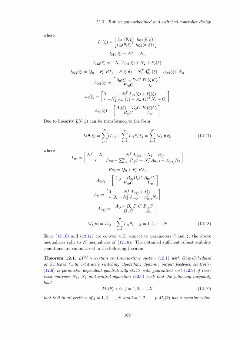
12.3. Robust gain-scheduled and switched controller design
where
L0(ξ) =
[l011(θ, ξ) l012(θ, ξ)l12(θ, ξ)T l022(θ, ξ))
]l011(ξ) = NT
1 +N1
l012(ξ) = −NT1 A0cl(ξ) +N2 + P0(ξ)
l022(ξ) = Q0 + F Tc RFc + P (ξ, θ)−NT2 A
T0cl(ξ)−A0cl(ξ)
TN2
A0cl(ξ) =
[A0(ξ) +DcC B0(ξ)Cc
Bc0C Ac0
]Li(ξ) =
[0 −NT
1 Aicl(ξ) + Pi(ξ)∗ −NT
2 Aicl(ξ)−Aicl(ξ)TN2 +Qi
]Aicl(ξ) =
[Ai(ξ) +DcC Bi(ξ)Cc
BciC Aci
]Due to linearity L(θ, ξ) can be transformed to the form
L(θ, ξ) =
N∑j=1
(L0j +
p∑i=1
Lijθi)ξj =
N∑j=1
Mj(θ)ξj (12.17)
where
L0j =
[NT
1 +N1 −NT1 A0clj +N2 + P0j
∗ Pe0 +∑p
i=1 Pij θi −NT2 A0clj −AT0cljN2
]Pe0 = Q0 + F Tc RFc
A0clj =
[A0j +B0jDcC B0jCc
Bc0C Ac0
]Lij =
[0 −NT
1 Aiclj + Pij∗ Qi −NT
2 Aiclj −ATicljN2
]Aiclj =
[Aij +BijDcC BijCc
BciC Aci
]
Mj(θ) = L0j +
p∑i=1
Lijθi, j = 1, 2, . . . , N (12.18)
Since (12.16) and (12.17) are convex with respect to parameters θ and ξ, the above
inequalities split to N inequalities of (12.18). The obtained sufficient robust stability
conditions are summarized in the following theorem.
Theorem 12.1. LPV uncertain continuous-time system (12.1) with Gain-Scheduled
or Switched (with arbitrarily switching algorithm) dynamic output feedback controller
(12.6) is parameter dependent quadratically stable with guaranteed cost (12.9) if there
exist matrices N1, N2 and control algorithm (12.6) such that the following inequality
hold
Mj(θ) < 0, j = 1, 2, . . . , N (12.19)
that is if in all vertices of j = 1, 2, . . . , N and i = 1, 2, . . . , p Mj(θ) has a negative value.
169
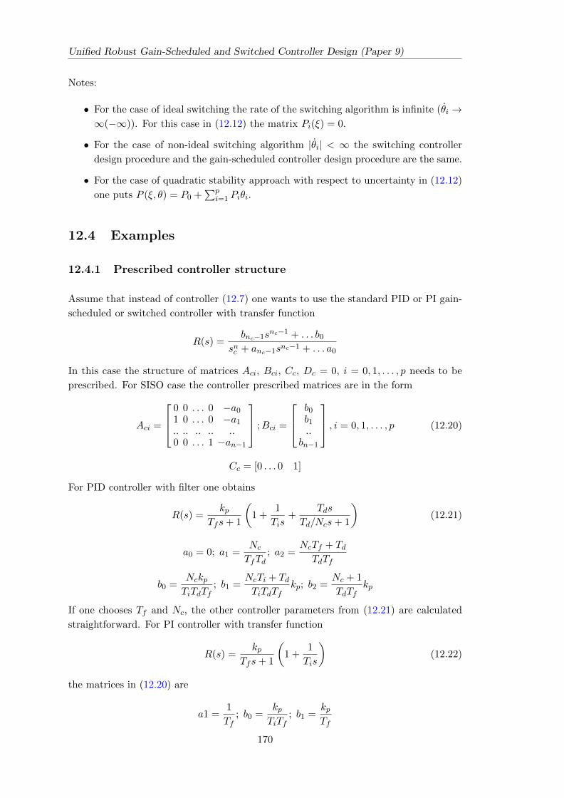
Unified Robust Gain-Scheduled and Switched Controller Design (Paper 9)
Notes:
• For the case of ideal switching the rate of the switching algorithm is infinite (θi →∞(−∞)). For this case in (12.12) the matrix Pi(ξ) = 0.
• For the case of non-ideal switching algorithm |θi| < ∞ the switching controller
design procedure and the gain-scheduled controller design procedure are the same.
• For the case of quadratic stability approach with respect to uncertainty in (12.12)
one puts P (ξ, θ) = P0 +∑p
i=1 Piθi.
12.4 Examples
12.4.1 Prescribed controller structure
Assume that instead of controller (12.7) one wants to use the standard PID or PI gain-
scheduled or switched controller with transfer function
R(s) =bnc−1s
nc−1 + . . . b0snc + anc−1snc−1 + . . . a0
In this case the structure of matrices Aci, Bci, Cc, Dc = 0, i = 0, 1, . . . , p needs to be
prescribed. For SISO case the controller prescribed matrices are in the form
Aci =
0 0 . . . 0 −a0
1 0 . . . 0 −a1
.. .. .. .. ..0 0 . . . 1 −an−1
;Bci =
b0b1..
bn−1
, i = 0, 1, . . . , p (12.20)
Cc = [0 . . . 0 1]
For PID controller with filter one obtains
R(s) =kp
Tfs+ 1
(1 +
1
Tis+
Tds
Td/Ncs+ 1
)(12.21)
a0 = 0; a1 =Nc
TfTd; a2 =
NcTf + TdTdTf
b0 =NckpTiTdTf
; b1 =NcTi + TdTiTdTf
kp; b2 =Nc + 1
TdTfkp
If one chooses Tf and Nc, the other controller parameters from (12.21) are calculated
straightforward. For PI controller with transfer function
R(s) =kp
Tfs+ 1
(1 +
1
Tis
)(12.22)
the matrices in (12.20) are
a1 =1
Tf; b0 =
kpTiTf
; b1 =kpTf
170
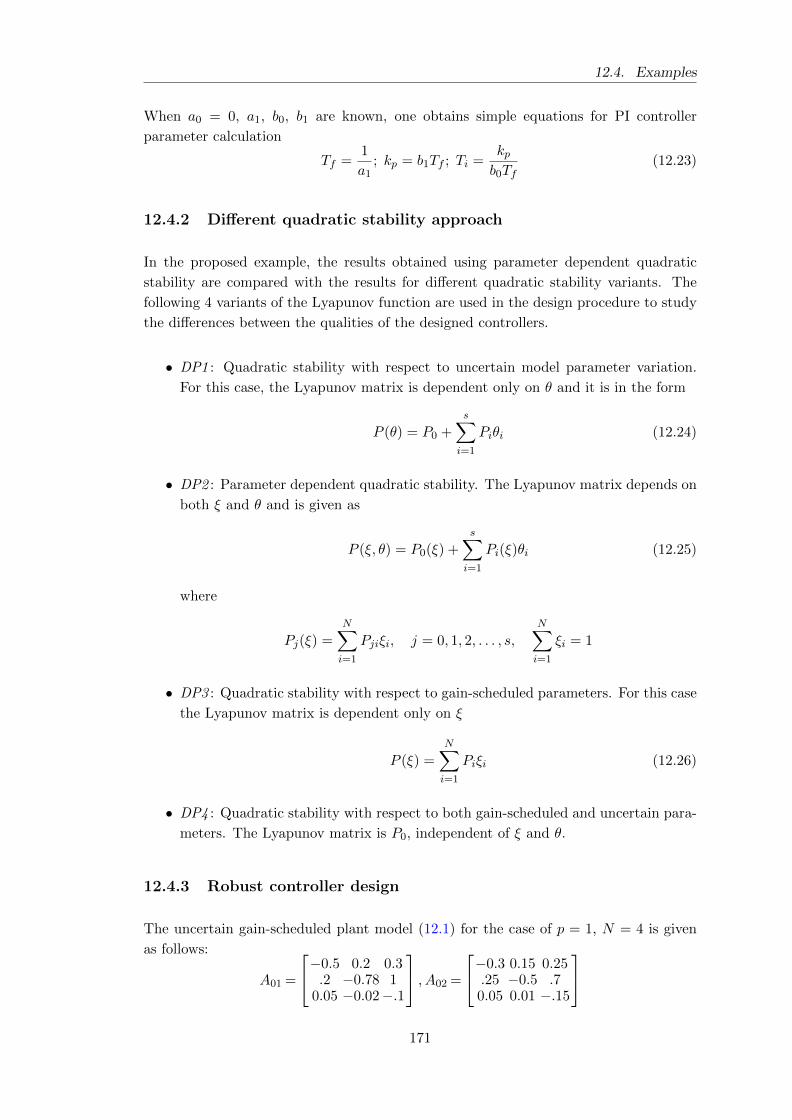
12.4. Examples
When a0 = 0, a1, b0, b1 are known, one obtains simple equations for PI controller
parameter calculation
Tf =1
a1; kp = b1Tf ; Ti =
kpb0Tf
(12.23)
12.4.2 Different quadratic stability approach
In the proposed example, the results obtained using parameter dependent quadratic
stability are compared with the results for different quadratic stability variants. The
following 4 variants of the Lyapunov function are used in the design procedure to study
the differences between the qualities of the designed controllers.
• DP1 : Quadratic stability with respect to uncertain model parameter variation.
For this case, the Lyapunov matrix is dependent only on θ and it is in the form
P (θ) = P0 +
s∑i=1
Piθi (12.24)
• DP2 : Parameter dependent quadratic stability. The Lyapunov matrix depends on
both ξ and θ and is given as
P (ξ, θ) = P0(ξ) +s∑i=1
Pi(ξ)θi (12.25)
where
Pj(ξ) =N∑i=1
Pjiξi, j = 0, 1, 2, . . . , s,N∑i=1
ξi = 1
• DP3 : Quadratic stability with respect to gain-scheduled parameters. For this case
the Lyapunov matrix is dependent only on ξ
P (ξ) =N∑i=1
Piξi (12.26)
• DP4 : Quadratic stability with respect to both gain-scheduled and uncertain para-
meters. The Lyapunov matrix is P0, independent of ξ and θ.
12.4.3 Robust controller design
The uncertain gain-scheduled plant model (12.1) for the case of p = 1, N = 4 is given
as follows:
A01 =
−0.5 0.2 0.3.2 −0.78 1
0.05 −0.02−.1
, A02 =
−0.3 0.15 0.25.25 −0.5 .70.05 0.01 −.15
171
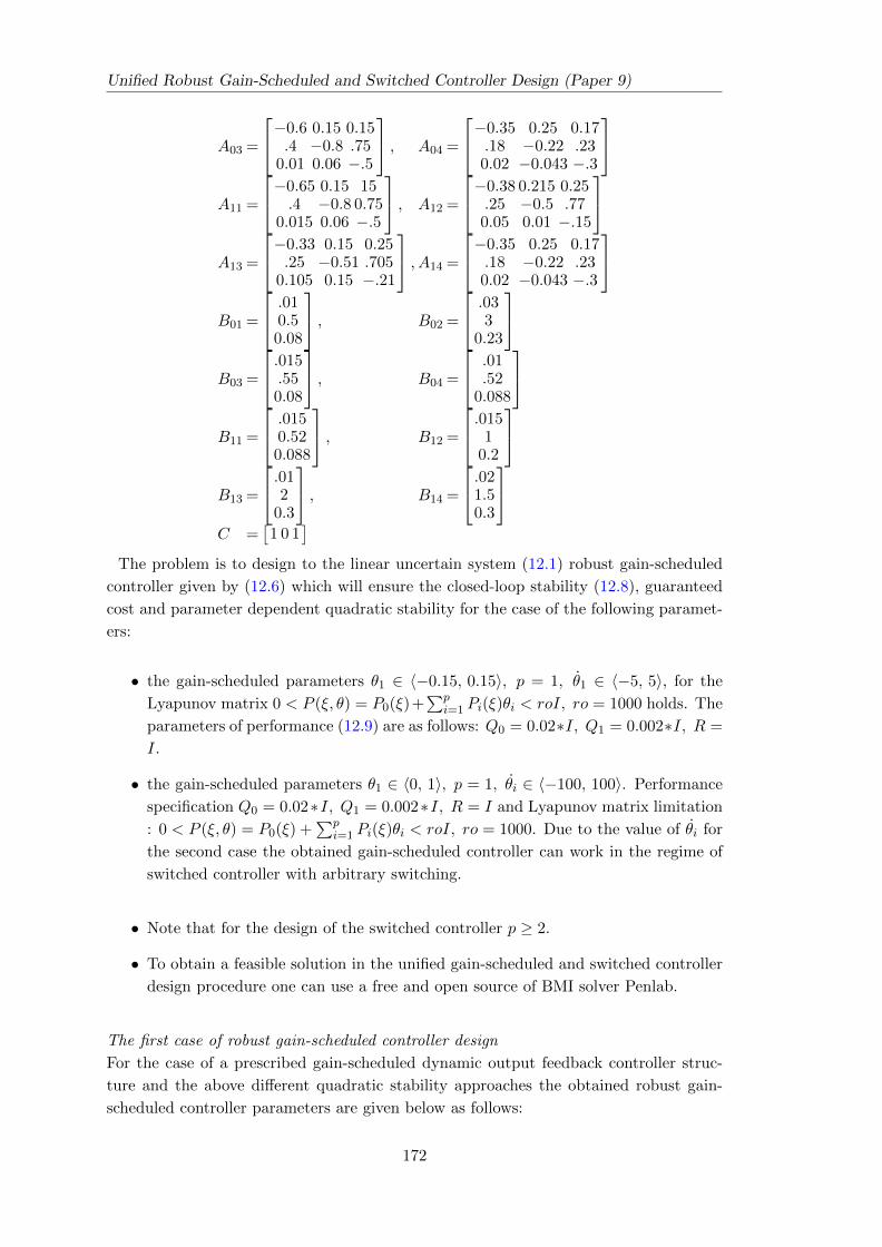
Unified Robust Gain-Scheduled and Switched Controller Design (Paper 9)
A03 =
−0.6 0.15 0.15.4 −0.8 .75
0.01 0.06 −.5
, A04 =
−0.35 0.25 0.17.18 −0.22 .230.02 −0.043 −.3
A11 =
−0.65 0.15 15.4 −0.8 0.75
0.015 0.06 −.5
, A12 =
−0.38 0.215 0.25.25 −0.5 .770.05 0.01 −.15
A13 =
−0.33 0.15 0.25.25 −0.51 .705
0.105 0.15 −.21
, A14 =
−0.35 0.25 0.17.18 −0.22 .230.02 −0.043 −.3
B01 =
.010.50.08
, B02 =
.033
0.23
B03 =
.015.550.08
, B04 =
.01.52
0.088
B11 =
.0150.520.088
, B12 =
.0151
0.2
B13 =
.012
0.3
, B14 =
.021.50.3
C =
[1 0 1
]The problem is to design to the linear uncertain system (12.1) robust gain-scheduled
controller given by (12.6) which will ensure the closed-loop stability (12.8), guaranteed
cost and parameter dependent quadratic stability for the case of the following paramet-
ers:
• the gain-scheduled parameters θ1 ∈ 〈−0.15, 0.15〉, p = 1, θ1 ∈ 〈−5, 5〉, for the
Lyapunov matrix 0 < P (ξ, θ) = P0(ξ)+∑p
i=1 Pi(ξ)θi < roI, ro = 1000 holds. The
parameters of performance (12.9) are as follows: Q0 = 0.02∗I, Q1 = 0.002∗I, R =
I.
• the gain-scheduled parameters θ1 ∈ 〈0, 1〉, p = 1, θi ∈ 〈−100, 100〉. Performance
specification Q0 = 0.02∗I, Q1 = 0.002∗I, R = I and Lyapunov matrix limitation
: 0 < P (ξ, θ) = P0(ξ) +∑p
i=1 Pi(ξ)θi < roI, ro = 1000. Due to the value of θi for
the second case the obtained gain-scheduled controller can work in the regime of
switched controller with arbitrary switching.
• Note that for the design of the switched controller p ≥ 2.
• To obtain a feasible solution in the unified gain-scheduled and switched controller
design procedure one can use a free and open source of BMI solver Penlab.
The first case of robust gain-scheduled controller design
For the case of a prescribed gain-scheduled dynamic output feedback controller struc-
ture and the above different quadratic stability approaches the obtained robust gain-
scheduled controller parameters are given below as follows:
172
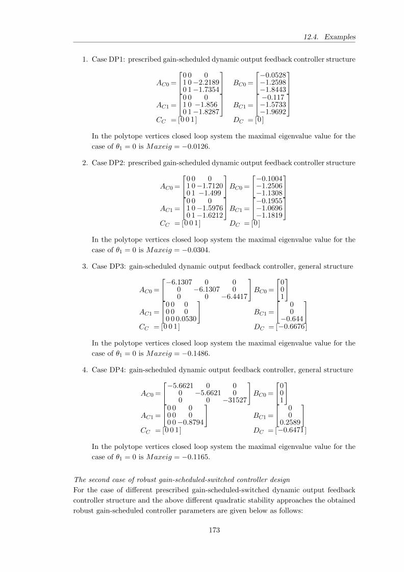
12.4. Examples
1. Case DP1: prescribed gain-scheduled dynamic output feedback controller structure
AC0 =
[0 0 01 0−2.21890 1−1.7354
]BC0 =
[−0.0528−1.2598−1.8443
]
AC1 =
[0 0 01 0 −1.8560 1−1.8287
]BC1 =
[ −0.117−1.5733−1.9692
]CC = [0 0 1] DC = [0]
In the polytope vertices closed loop system the maximal eigenvalue value for the
case of θ1 = 0 is Maxeig = −0.0126.
2. Case DP2: prescribed gain-scheduled dynamic output feedback controller structure
AC0 =
[0 0 01 0−1.71200 1 −1.499
]BC0 =
[−0.1004−1.2506−1.1308
]
AC1 =
[0 0 01 0−1.59760 1−1.6212
]BC1 =
[−0.1955−1.0696−1.1819
]CC = [0 0 1] DC = [0]
In the polytope vertices closed loop system the maximal eigenvalue value for the
case of θ1 = 0 is Maxeig = −0.0304.
3. Case DP3: gain-scheduled dynamic output feedback controller, general structure
AC0 =
[−6.1307 0 00 −6.1307 00 0 −6.4417
]BC0 =
[001
]
AC1 =
[0 0 00 0 00 0 0.0530
]BC1 =
[00
−0.644
]CC = [0 0 1] DC = [−0.6676]
In the polytope vertices closed loop system the maximal eigenvalue value for the
case of θ1 = 0 is Maxeig = −0.1486.
4. Case DP4: gain-scheduled dynamic output feedback controller, general structure
AC0 =
[−5.6621 0 00 −5.6621 00 0 −31527
]BC0 =
[001
]
AC1 =
[0 0 00 0 00 0−0.8794
]BC1 =
[00
0.2589
]CC = [0 0 1] DC = [−0.6471]
In the polytope vertices closed loop system the maximal eigenvalue value for the
case of θ1 = 0 is Maxeig = −0.1165.
The second case of robust gain-scheduled-switched controller design
For the case of different prescribed gain-scheduled-switched dynamic output feedback
controller structure and the above different quadratic stability approaches the obtained
robust gain-scheduled controller parameters are given below as follows:
173
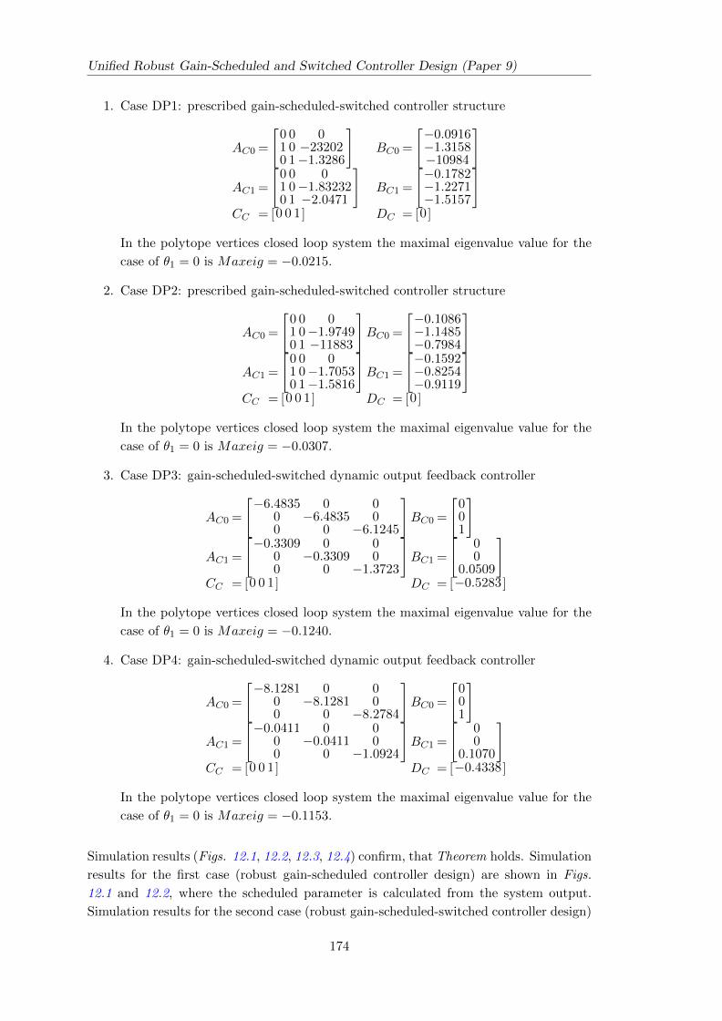
Unified Robust Gain-Scheduled and Switched Controller Design (Paper 9)
1. Case DP1: prescribed gain-scheduled-switched controller structure
AC0 =
[0 0 01 0 −232020 1−1.3286
]BC0 =
[−0.0916−1.3158−10984
]
AC1 =
[0 0 01 0−1.832320 1 −2.0471
]BC1 =
[−0.1782−1.2271−1.5157
]CC = [0 0 1] DC = [0]
In the polytope vertices closed loop system the maximal eigenvalue value for the
case of θ1 = 0 is Maxeig = −0.0215.
2. Case DP2: prescribed gain-scheduled-switched controller structure
AC0 =
[0 0 01 0−1.97490 1 −11883
]BC0 =
[−0.1086−1.1485−0.7984
]
AC1 =
[0 0 01 0−1.70530 1−1.5816
]BC1 =
[−0.1592−0.8254−0.9119
]CC = [0 0 1] DC = [0]
In the polytope vertices closed loop system the maximal eigenvalue value for the
case of θ1 = 0 is Maxeig = −0.0307.
3. Case DP3: gain-scheduled-switched dynamic output feedback controller
AC0 =
[−6.4835 0 00 −6.4835 00 0 −6.1245
]BC0 =
[001
]
AC1 =
[−0.3309 0 00 −0.3309 00 0 −1.3723
]BC1 =
[00
0.0509
]CC = [0 0 1] DC = [−0.5283]
In the polytope vertices closed loop system the maximal eigenvalue value for the
case of θ1 = 0 is Maxeig = −0.1240.
4. Case DP4: gain-scheduled-switched dynamic output feedback controller
AC0 =
[−8.1281 0 00 −8.1281 00 0 −8.2784
]BC0 =
[001
]
AC1 =
[−0.0411 0 00 −0.0411 00 0 −1.0924
]BC1 =
[00
0.1070
]CC = [0 0 1] DC = [−0.4338]
In the polytope vertices closed loop system the maximal eigenvalue value for the
case of θ1 = 0 is Maxeig = −0.1153.
Simulation results (Figs. 12.1, 12.2, 12.3, 12.4) confirm, that Theorem holds. Simulation
results for the first case (robust gain-scheduled controller design) are shown in Figs.
12.1 and 12.2, where the scheduled parameter is calculated from the system output.
Simulation results for the second case (robust gain-scheduled-switched controller design)
174
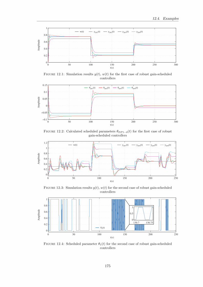
12.4. Examples
Figure 12.1: Simulation results y(t), w(t) for the first case of robust gain-scheduledcontrollers
Figure 12.2: Calculated scheduled parameters θDP1−4(t) for the first case of robustgain-scheduled controllers
Figure 12.3: Simulation results y(t), w(t) for the second case of robust gain-scheduledcontrollers
Figure 12.4: Scheduled parameter θ1(t) for the second case of robust gain-scheduledcontrollers
175
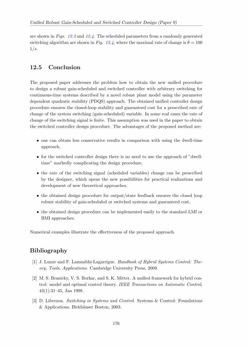
Unified Robust Gain-Scheduled and Switched Controller Design (Paper 9)
are shown in Figs. 12.3 and 12.4. The scheduled parameters from a randomly generated
switching algorithm are shown in Fig. 12.4, where the maximal rate of change is θ = 100
1/s.
12.5 Conclusion
The proposed paper addresses the problem how to obtain the new unified procedure
to design a robust gain-scheduled and switched controller with arbitrary switching for
continuous-time systems described by a novel robust plant model using the parameter
dependent quadratic stability (PDQS) approach. The obtained unified controller design
procedure ensures the closed-loop stability and guaranteed cost for a prescribed rate of
change of the system switching (gain-scheduled) variable. In some real cases the rate of
change of the switching signal is finite. This assumption was used in the paper to obtain
the switched controller design procedure. The advantages of the proposed method are:
• one can obtain less conservative results in comparison with using the dwell-time
approach,
• for the switched controller design there is no need to use the approach of ”dwell-
time” markedly complicating the design procedure,
• the rate of the switching signal (scheduled variables) change can be prescribed
by the designer, which opens the new possibilities for practical realizations and
development of new theoretical approaches,
• the obtained design procedure for output/state feedback ensures the closed loop
robust stability of gain-scheduled or switched systems and guaranteed cost,
• the obtained design procedure can be implemented easily to the standard LMI or
BMI approaches.
Numerical examples illustrate the effectiveness of the proposed approach.
Bibliography
[1] J. Lunze and F. Lamnabhi-Lagarrigue. Handbook of Hybrid Systems Control: The-
ory, Tools, Applications. Cambridge University Press, 2009.
[2] M. S. Branicky, V. S. Borkar, and S. K. Mitter. A unified framework for hybrid con-
trol: model and optimal control theory. IEEE Transactions on Automatic Control,
43(1):31–45, Jan 1998.
[3] D. Liberzon. Switching in Systems and Control. Systems & Control: Foundations
& Applications. Birkhauser Boston, 2003.
176
Bibliography
[4] J. Lygeros. An Overview of Research Areas in Hybrid Control. In 44th IEEE
Conference on Decision and Control, 2005 and 2005 European Control Conference.
CDC-ECC ’05., pages 5600–5605, 2005.
[5] H. Lin and P. Antsaklis. Stability and Stabilizability of Switched Linear Systems:
A Survey of Recent Results. IEEE Trans. on AC, 54(2):308–322, 2009.
[6] J. Geromel and P. Colaneri. Stability and Stabilization of Continuous-Time
Switched Linear Systems. SIAM Journal on Control and Optimization, 45(5):1915–
1930, 2006.
[7] L. I. Allerhand and U. Shaked. Robust Stability and Stabilization of Linear Switched
Systems With Dwell Time. IEEE Transactions on Automatic Control, 56(2):381–
386, Feb 2011.
[8] L. Zhao, X. Zhang and M. Lin. Stability of switched positive linear systems with
average dwell time switching. Automatica, 48(10):1132–1137, 2012.
[9] R. Guo and Y. Wang. Stability analysis for a class of switched linear systems. Asian
Journal of control, 14(3):817–826, 2012.
[10] M. Cao and A.S. Morse. Dwell-time switching. Systems and Control Letters,
59(1):57–65, 2010.
[11] D. J. Leith and W. E. Leithead. Survey of Gain-Scheduling analysis and design.
Inter Journal of Control, 73(11):1001–1025, 2000.
[12] W. J. Rugh and J. S. Shamma. Research on gain scheduling: Survey paper. Auto-
matica, 36(7):1401–1425, 2000.
[13] V. Vesely and A. Ilka Gain-scheduled PID controller design. Journal of Process
Control, 23(8):1141–1148, September 2013.
[14] V. Rosinova, D. Vesely and V. Kucera. A necessary and sufficient conditions for
static output feedback stabilizibility of linear discrete-time systems. Kybernetika,
39(4):447–459, 2003.
[15] V. M. Kuncevic and M. M. Lycak. Control System Design using Lyapunov Function
Approach. Nauka, Moskau, 1977 in Russian, 1977.
177

13
Concluding remarks
13.1 Brief overview
This thesis deals with controller design for nonlinear systems. The controller is given in
a feedback structure that is, the controller has information about the system and uses
it to influence the system. The nonlinear system is transformed to a linear parameter-
varying system which is used for controller design, i.e. gain-scheduled controller design.
The gain-scheduled controller synthesis presented in this thesis is based on the Lyapunov
theory of stability as well as on the Bellman-Lyapunov function. To achieve a perform-
ance quality, a quadratic cost function and its modifications known from LQ theory are
used. The obtained gain-scheduled controller guarantees the closed-loop stability and
the guaranteed cost. The main results for controller synthesis are in the form of bilin-
ear matrix inequalities and/or linear matrix inequalities. For controller synthesis, one
can use a free and open source BMI solver PenLab or LMI solvers LMILab, SDPT3 or
SeDuMi.
13.2 Closing remarks and future works
The main goal for this thesis (and also to our research in last 2,5 – 3 years) was to find a
systematic controller design approach for uncertain nonlinear systems, which guarantees
the closed-loop stability and guaranteed cost with considering input/output constraints,
all this without on-line optimization and need of high-performance industrial computers.
We tried to select those publications which most closely reflect the achieved results. The
first included paper (Chapter 4) presents a simple gain-scheduled controller design for
nonlinear systems which guarantees the closed-loop stability and guaranteed cost. One
can include the maximal value of the rate of gain-scheduled parameter changes which
allows obtaining the controller with a given performance and decreased conservative-
ness. In the next chapter (Chapter 5), one can find a simple modification of these
results, where a new quadratic cost function is used, where weighting matrices are time-
varying and depending on scheduled parameter. Using these original variable weighting
179
13. Concluding remarks
matrices, we can affect performance quality separately in each working point and we can
tune the system to the desired condition through all parameter changes. Chapters 6, 7
present the robust versions of the obtained results from Chapters 4, 5, where in Chapter
6 the design procedure is transformed from the bilinear matrix inequality form to lin-
ear matrix inequality, which caused that our controller synthesis works for high order
systems. In Chapter 8, a simplified version of the robust controller design in discrete
time domain is presented, where a new LPV description of T1DM Bergman’s minimal
model with two additional subsystems (absorption of digested carbohydrates and sub-
cutaneous insulin absorption) is created. The controller synthesis in this paper is also
transformed to LMI problem. In Chapters 9 and 10, gain-scheduled controller designs
adopted to switched control are presented in continuous time. In the proposed design
procedures there is no need to use the notion of the ”dwell-time” for arbitrary switching,
which significantly simplifies the switched controller design compared to approaches in
the literatures. In Chapter 11, a novel gain scheduling based model predictive control-
ler design procedure for nonlinear systems is presented for finite and infinite prediction
horizons with considering input/output constraints. Finally, a novel unified robust gain-
scheduled and switched controller design approach is presented in Chapter 12, where the
conservativeness from multi-convexity is eliminated.
The stated objectives (in Chapter 1) were reached successfully but there are still many
unsolved problems. For example, in this thesis it is hypothesized that the scheduled
parameters can be measured and the measurement is accurate. It is true that if one
uses the robust version, then the measurement inaccuracy can be covered as model
uncertainty but this should be studied in more detail. Furthermore, it would be good
to study how information from disturbances can be used to improve the performance
quality under disturbances. Moreover, it would be an interesting study how to reduce
the time required to controller synthesis because it is well known that the time required
for controller design using LMI and especially BMI solvers rapidly increases for higher
order systems. It follows that this thesis opens new possibilities for further studies and
research in this specific area.
180
Appendix A
List of publications
Original research papers in international scientific journals
(peer- reviewed)
[1] VESELY, Vojtech – ILKA, Adrian. Gain-Scheduled PID Controller Design.
Journal of Process Control, 2013, vol. 23, p. 1141-1148.
[2] ILKA, Adrian – VESELY, Vojtech. Robust Gain-Scheduled Controller Design
for Uncertain LPV systems: Affine Quadratic Stability Approach. Journal of
Electrical Systems and Information Technology, 2014, vol. 1, no. 1, p. 45-57.
[3] ILKA, Adrian – VESELY, Vojtech. Gain-Scheduled Controller Design: Variable
Weighting Approach. Journal of Electrical Engineering, 2014, vol. 65, no. 2, p.
116-120.
[4] VESELY, Vojtech – ILKA, Adrian. Robust Gain-Scheduled PID Controller Design
for Uncertain LPV Systems. Journal of Electrical Engineering, 2015, vol. 66, no.
1, p. 19-26.
[5] VESELY, Vojtech – ILKA, Adrian. Design of Robust Gain-Scheduled PI Control-
lers. Journal of the Franklin Institute, 2015, vol. 352, no. 1, p. 1476-1494.
[6] ILKA, Adrian – OTTINGER, Ivan – LUDWIG, Tomas – TARNIK, Marian –
VESELY, Vojtech – MIKLOVICOVA, Eva – MURGAS, Jan. Robust Controller
Design for T1DM Individualized Model: Gain Scheduling Approach. International
Review of Automatic Control (I.RE.A.CO), 2015, vol. 8, no. 2, p. 155-162.
[7] VESELY, Vojtech – ILKA, Adrian. Novel Approach to Switched Controller Design
for Linear Continuous-Time Systems. Accepted in Asian Journal of Control, Ac-
ceptance day: 22. May, 2015.
181
Appendix A. List of publications
Published contributions on scientific conferences or sym-
posiums (peer-reviewed)
[1] HOLIC, Ivan -– ILKA, Adrian. Robust State Feedback Controller Design for DC-
Motor System. Oxford: Elsevier, 2013. Advances in Control Education – ACE
2013: 10th IFAC Symposium on Advances in Control Education. Scheffield, UK,
August 28-30, 2013, p. 120-125. ISBN 978-3-902823-43-4.
[2] VOZAK, Daniel – ILKA, Adrian. Application of Unstable System in Education of
Modern Control Methods. Oxford: Elsevier, 2013. Advances in Control Education
– ACE 2013: 10th IFAC Symposium on Advances in Control Education. Scheffield,
UK, August 28-30, 2013, p. 114-119. ISBN 978-3-902823-43-4.
[3] VESELY, Vojtech – ROSINOVA, Danica – ILKA, Adrian. Decentralized Gain
Scheduling Controller Design: Polytopic System Approach. Shanghai: IFAC, 2013.
Large Scale Complex Systems Theory and Applications: 13th IFAC Symposium.
Shanghai, China, July 7-10, 2013, p. 401-406. ISBN 978-3-902823-39-7.
[4] ILKA, Adrian – VESELY, Vojtech. Discrete Gain-Scheduled Controller Design:
Guaranteed Cost and Affine Quadratic Stability Approach. Proceedings of the
International Conference on Innovative Technologies IN-TECH 2013, Budapest,
Hungary 10.-13.09.2013, p. 157-160. ISBN 978-953-6326-88-4.
[5] VESELY, Vojtech – ILKA, Adrian. Gain-Scheduled Controller design: MIMO
Systems. Proceedings of the 14th International Carpathian Control Conference
ICCC 2013. Rytro, Poland, May 26-29, 2013, p. 417-422. ISBN 978-1-4673-4489-
0.
[6] ILKA, Adrian – VESELY, Vojtech. Discrete gain-scheduled controller design:
Variable weighting approach. Proceedings of the 15th International Carpathian
Control Conference ICCC 2014. Velke Karlovice, Czech Republic, May 28-30,
2014, p. 186-191. ISBN 978-1-4799-3527-7.
[7] VESELY, Vojtech – ILKA, Adrian. PID robust gain-scheduled controller design.
Proceedings of the 13th European Control Conference 2014, June 24-27, 2014,
Strasbourg, France, p. 2756-2761. ISBN 978-3-9524269-2-0.
[8] VESELY, Vojtech – ILKA, Adrian. Gain-Scheduled Controller Design: Guar-
anteed Quality Approach. Proceedings of the 19th International Conference on
Process Control 2013. Strbske Pleso, Slovakia, June 18-21, 2013, p. 456-461.
ISBN 978-80-227-3951-1.
[9] VESELY, Vojtech – ILKA, Adrian – KOZAKOVA, Alena. Frequency Domain
Gain Scheduled Controller Design for SISO Systems. Proceedings of the 19th
International Conference on Process Control 2013. Strbske Pleso, Slovakia, June
18-21, 2013, p. 439-444. ISBN 978-80-227-3951-1.
182
Appendix A. List of publications
[10] ILKA, Adrian – VESELY, Vojtech. Gain-Scheduled Controller Design: Vari-
able Weighting Approach. Bratislava. 15th Conference of Doctoral Students
ELITECH´13. Bratislava, Slovakia, 5 June 2013, p. 1-6. ISBN 978-80-227-3947-4.
[11] ILKA, Adrian – ERNEK, Martin. Modeling and Control System of Wind Power
Plants with Pumped Storage Hydro Power Plant. Renewable Energy Sources 2013:
4th International Scientific Conference OZE 2013. Tatranske Matliare, Slovakia,
May 21-23, 2013, p. 495-500. ISBN 978-80-89402-64-9.
[12] ILKA, Adrian – VESELY, Vojtech. Robust Gain-Scheduled Controller Design for
Uncertain LPV Systems: Quadratic Stability Approach. International Conference
on Cybernetics and Informatics SSKI 2014. Oscadnica, Slovakia, 5.-8. 2. 2014,
ISBN 978-80-227-4122-4.
[13] VESELY, Vojtech – ILKA, Adrian. Switched system controller design: Quadratic
stability approach. International Conference on Cybernetics and Informatics SSKI
2014; Oscadnica, Slovakia, 5.-8. 2. 2014, ISBN 978-80-227-4122-4.
[14] ILKA, Adrian – VESELY, Vojtech. Decentralized gain-scheduled PSS design on
the base of experimental dates. Proceedings of the 11th International Scientific
Conference on Control of Power Systems 2014; Tatranske Matliare, Slovakia; 20-22
May 2014, p. 15-20. ISBN 978-80-89402-72-4.
[15] ILKA, Adrian – VESELY, Vojtech. Robust discrete gain-scheduled controller
design: LMI approach. 16th Conference of Doctoral Students ELITECH´14; Brat-
islava, Slovakia, 4 June 2014, ISBN 978-80-227-4171-2.
[16] VESELY, Vojtech – ILKA, Adrian. Robust Switched Controller Design for Non-
linear Continuous Systems. Accepted to the 1st IFAC Conference on Modeling,
Identification and Control of Nonlinear Systems – MINCON 2015, Saint Peters-
burg, Russian Federation, June 24-26, 2015, Acceptance day: 16. March, 2015.
[17] ILKA, Adrian – VESELY, Vojtech. Gain-Scheduled MPC Design for Nonlinear
Systems with Input Constraints. Accepted to the 1st IFAC Conference on Mod-
eling, Identification and Control of Nonlinear Systems – MINCON 2015, Saint
Petersburg, Russian Federation, June 24-26, 2015, Acceptance day: 16. March,
2015.
[18] VESELY, Vojtech – ILKA, Adrian. Robust Controller Design with Input Con-
straints, Time Domain Approach. Accepted to the 8th IFAC Symposium on Ro-
bust Control Design – ROCOND 2015, Bratislava, Slovakia, July 15-17, 2015,
Acceptance day: 20. April, 2015.
[19] ILKA, Adrian – LUDWIG, Tomas – OTTINGER, Ivan – TARNIK, Marian –
MIKLOVICOVA, Eva – VESELY, Vojtech – MURGAS, Jan., Ivan. Robust Gain-
Scheduled Controller Design for T1DM Individualised Model. Accepted to the
8th IFAC Symposium on Robust Control Design – ROCOND 2015, Bratislava,
Slovakia, July 15-17, 2015, Acceptance day: 20. April, 2015.
183
Appendix A. List of publications
[20] ILKA, Adrian – VESELY, Vojtech. Robust Discrete Gain-Scheduled Controller
Design for Uncertain LPV Systems. Accepted to the 20th International Conference
on Process Control, Strbske pleso, Slovak Republic, June 9-12, 2015, Acceptance
day: 20. April, 2015.
[21] ILKA, Adrian – VESELY, Vojtech. Observer-Based Output Feedback Gain-
Scheduled Controller Design. Accepted to the 20th International Conference on
Process Control, Strbske pleso, Slovak Republic, June 9-12, 2015, Acceptance day:
20. April, 2015.
[22] ILKA, Adrian – VESELY, Vojtech. Gain-Scheduled Model Predictive Controller
Design. Accepted to the 17th Conference of Doctoral Students, ELITECH´15;
Bratislava, Slovakia, May 25, 2015, Acceptance day: 11. May, 2015.
Original research papers submitted to international sci-
entific journals (peer-reviewed)
[1] ILKA, Adrian – VESELY, Vojtech. Decentralized Power System Stabilizer Design:
Gain Scheduling Approach. Submitted to the Journal of Electrical Systems and
Information Technology. Submitted on 29. March, 2015.
[2] VESELY, Vojtech – ILKA, Adrian. Output Feedback Control of Switched Nonlin-
ear Systems: A Gain Scheduling Approach. Submitted to the Journal of Electrical
Engineering, Submitted on 7. May, 2014.
[3] ILKA, Adrian – VESELY, Vojtech. Unified Robust Gain-Scheduled and Switched
Controller Design for Linear Continuous-Time Systems. Submitted to the journal
International Review of Automatic Control (I.RE.A.CO). Submitted on 25. May,
2015.
[4] ILKA, Adrian – VESELY, Vojtech. Robust Switched Controller Design for Linear
Continuous-Time Systems. Submitted to the journal Archives of Control Sciences,
Submitted on 25. May, 2015.
Other publications
[1] ILKA, Adrian. Modeling and Control of Wind Turbine. BSc thesis, Slovak Uni-
versity of Technology in Bratislava 2010, 86 p., in Slovak.
[2] ILKA, Adrian. Modeling and Control System of Wind Power Plants with Pumped
Storage Hydro Power Plant, MSc thesis, Slovak University of Technology in Brat-
islava, 2012, 128 p., in Slovak.
[3] ILKA, Adrian – ERNEK, Martin. Modeling and Control of Wind Turbine using
MatLab/SimPowerSystems. Proceedings of the SVOC 2011, Bratislava, Slovakia,
4.5.2011, p. 355-361, ISBN 978-80-227-3508-7.
184