G3 - NASA · Brij Mohan V. Mandala, Graduate Research Assistant Year End Report for 1990 Prepared for National Aeronautics and Space Administration Langley Research Center Hampton,

oG3

G3©

o

©

t

DEPARTMENT OF ELECTRICAL & COMPUTER ENGINEERING

COLLEGE OF ENGINEERING & TECHNOLOGY/

OLD DOMINION UNIVERSITY _ _---_A:_:";:_/NORFOLK, VIRGINIA 23529

, _ , -r /J'r

ATAMM ENHANCEMENT AND MULTIPROCESSOR

PERFORMANCE EVALUATIONt

,/ /

/;

i

By

John W. Stoughton, Principal Investigator

Roland R. Mielke, Co-Principal Investigator

Sukhamoy Som, Research Associate

Rodrigo Obando, Graduate Research Assistant

Mahyar R. Malekpour, Graduate Research Assistant

Robert L. Jones III, Graduate Research Assistant

Brij Mohan V. Mandala, Graduate Research Assistant

Year End Report for 1990

Prepared forNational Aeronautics and Space Administration

Langley Research Center

Hampton, Virginia 23665

Under

Research Grant NCCI-136

Paul J. Hayes, Technical Monitor

ISD-Information Processing Technology Branch

" _ Mi _J

_:'r°r" , _- _._.r. l'7do - -_,l Oec. 19°0 (tJ1u,c_inion Univ. ) Ill n CSCL 0_ q

i'_o I-!47 go,

June 1991

https://ntrs.nasa.gov/search.jsp?R=19910015474 2019-03-14T22:30:00+00:00Z

DEPARTMENT OF ELECTRICAL & COMPUTER ENGINEERING

COLLEGE OF ENGINEERING & TECHNOLOGY

OLD DOMINION UNIVERSITY

NORFOLK, VIRGINIA 23529

ATAMM ENF,ANCEMENT AND MULTIPROCESSOR

PERFORMANCE EVALUATION

By

John W. Stoughton, Principal Investigator

Roland R. Mielke, Co-Principal Investigator

Sukhamoy Som, Research Associate

Rodrigo Obando, Graduate Research Assistant

Mahyar R. Malekpour, Graduate Research AssistantRobert L. Jones III, Graduate Research Assistant

Brij Mohan V. Mandala, Graduate Research Assistant

Year End Report for 1990

Prepared for

National Aeronautics and Space Administration

Langley Research Center

Hampton, Virginia 23665

Under

Research Grant NCCI-136

Paul J. Hayes, Technical Monitor

ISD-Information Processing Technology Branch

Submitted by the

Old Dominion University Research FoundationP.O. Box 6369

Norfolk, Virginia 23508-0369

June 1991

ATAMM ENHANCEMENT AND MULTIPROCESSOR PERFORMANCE

EVALUATION

CHAP'IER

1.

2.

°

°

TABLE OF CONTENTS

PAGE

INTRODUCTION ....................................................................... 1

THE ATAMM MODEL .............................................................. 5

2.0 Introduction .................................................................... 5

2.1 Model Description ......................................................... 5

2.2 Time Performance .......................................................... 9

2.2.1 Performance Measures .................................... 10

2.2.2 Graph Play and Resource Requirements ........ 11

2.2.3 ATAMM Performance Plane ......................... 13

ATAMM ENHANCEMENTS .................................................... 30

3.0 Introduction ................................................................... 30

3.1 Real-Time Control ......................................................... 30

3.2 Fault Tolerant Strategies ................................................ 32

3.2.1. TMR Implementation .................................... 32

3.2.2. Fault Detection and Recovery ....................... 37

ADM IMPLEMENTATION OF ATAMM ................................. 41

4.0 Introduction .................................................................... 41

4.1 ADM Architecture ......................................................... 41

(i)

4.2

4.2.1

4.2.2

4.2.3

AMOS Description ........................................................

Operating System Principles ..........................

Data Structures ................................................

Example ...........................................................

4.2.4 Functional Unit Operations ............................

4.3 1553B Software ..............................................................

4.4 IBM PC/386 Software ...................................................

5. ATAMM SUPPORT TOOLS ......................................................

6. RESEARCH STATUS .................................................................

REFERENCES ..............................................................................................

42

43

45

5O

52

55

60

97

101

105

(ii)

CHAPTERONE

INTRODUCTION

The purposeof this document is to describe progress of research to refine and

evaluate a new multicomputing system philosophy in a VHSIC technology based

multicomputer system during the period March 16, 1989 to December 31, 1990. This

research supports ongoing investigations being conducted at NASA Langley Research

Center concerning the insertion of VHSIC technology to potential future aerospace

applications. This is the year ending report for calendar year 1990 on the research

performed under Cooperative Agreement NCCl-136.

During the past four years, the authors and colleagues have conducted research

concerning the development of strategies for concurrent processing of complex

algorithms. A significant result of this work has been the development of a

multicomputer operating strategy for executing large-grained, decision-free algorithms

on data flow architectures. The operating strategy is expressed as a model for

concurrent processing called ATAMM for Algorithm To Architecture Mapping Model

[1, 2]. The model is significant because it identifies the control dialogue and data

flow required to implement a decomposed algorithm in a data flow architecture, and

because it provides a context for analytically predicting system time performance.

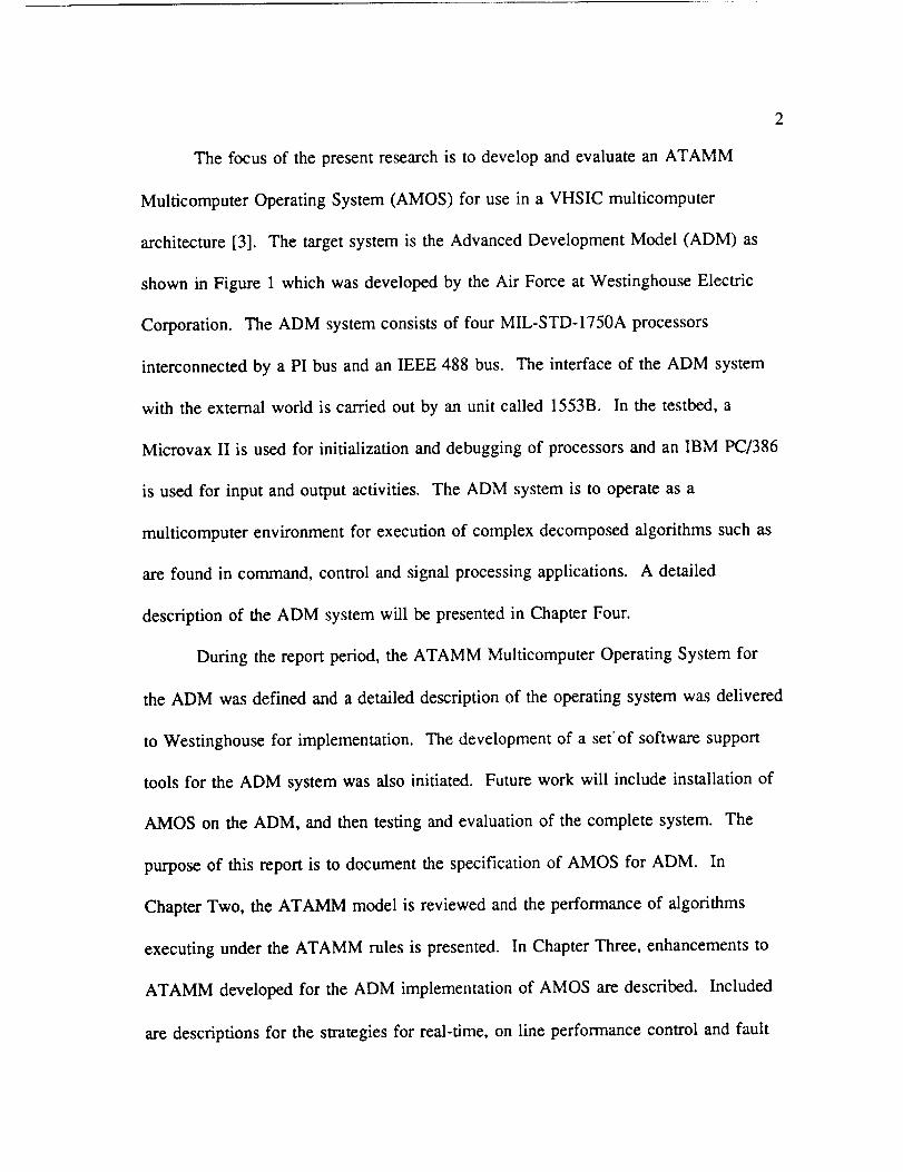
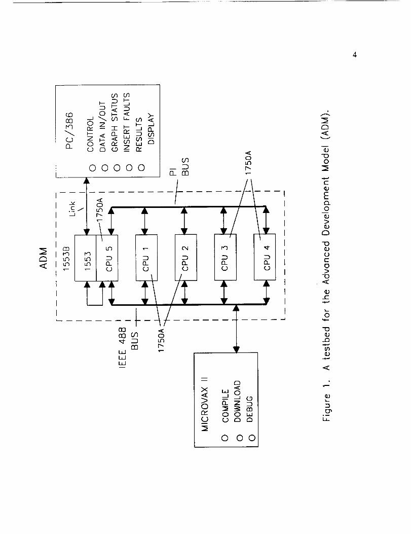
The focusof the presentresearchis to developandevaluatean ATAMM

MulticomputerOperatingSystem(AMOS) for use in a VHSIC multicomputer

architecture[3]. The targetsystemis the AdvancedDevelopmentModel (ADM) as

shownin Figure 1 which wasdevelopedby the Air Forceat WestinghouseElectric

Corporation. The ADM systemconsistsof four MIL-STD-1750A processors

interconnectedby a PI busandan IEEE488 bus. The interfaceof the ADM system

with the externalworld is carriedout by an unit called 1553B. In thetestbed,a

Microvax II is usedfor initialization anddebuggingof processorsandan IBM PC/386

is usedfor input and outputactivities. The ADM systemis to operateasa

multicomputerenvironmentfor executionof complexdecomposedalgorithmssuchas

are found in command,control andsignalprocessingapplications. A detailed

descriptionof the ADM systemwill bepresentedin ChapterFour.

During the report period, theATAMM MulticomputerOperatingSystemfor

theADM wasdefinedand adetaileddescriptionof the operatingsystemwasdelivered

to Westinghousefor implementation.The developmentof a set'of softwaresupport

tools for the ADM systemwasalsoinitiated. Futurework will include installationof

AMOS on the ADM, andthen testingandevaluationof the completesystem. The

purposeof this report is to documentthe specificationof AMOS for ADM. In

ChapterTwo, the ATAMM model is reviewedand theperformanceof algorithms

executingunderthe ATAMM rules is presented. In ChapterThree,enhancementsto

ATAMM developedfor the ADM implementationof AMOS aredescribed. Included

aredescriptionsfor the strategiesfor real-time,on line performancecontrol andfault

tolerance. The detailedspecificationfor AMOS andinput/outputcommunication

softwarearepresentedin ChapterFour. In ChapterFive, threesoftwaresupporttools

developedfor performanceanalysisin the ATAMM environmentaredescribed.The

report concludeswith a summaryof the statusof researchin ChapterSix.

The useof brandnamesin this report is for completeness,anddoesnot

indicateNASA endorsement.

3

,,m..<

COr,Q

(_)0._

J _ _J

ooogm

00000 _n 8O

O3

COWWW

n_

oL_

O

w 0

"5 _ m0 0 ','

0 O0

"5

-100

"5

C

E0

r_

-10

0c-O

r

0

C_)--

CHAPTER TWO

THE ATAMM MODEL

2.0 Introduction

The ATAMM model is reviewed briefly in this chapter. The definition of

ATAMM is presented and illustrated by example in Section 2.1. In Section 2.2, the

time performance of algorithms executing according to the ATAMM rules described.

Strategies are developed for generating operating conditions for predictable

performance based on the number of available computing resources.

2.1 Model Description

The ATAMM model consists of a set of Petri Net marked graphs which

incorporates general specifications of communication and processing associated with

the implementation of a decomposed, large-grained algorithm in a data-flow

architecture. In this section, the execution of a computational problem is represented

by the ATAMM model. Some familiarity with Petri Nets and marked graphs is

assumed [4]. A more detailed description of the ATAMM model and its

characteristics are found in [5, 6].

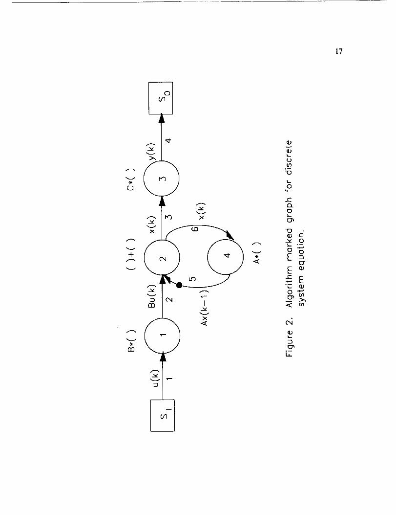
An algorithm marked graph (AMG) is a marked graph which represents a

specific algorithm decomposition. Transitions and places are represented as nodes

(vertices) and directed edges respectively. Vertices of the algorithm marked graph are

5

in a one-to-onecorrespondencewith eachoccurrenceof analgorithmoperation. The

transitiontimesrepresentthe computationaltimesof the respectivealgorithm

operations.The algorithmmarkedgraphcontainsanedge(i, j) directedfrom vertex i

to vertex j if the outputof vertex i is an input for vertexj. Edge(i, j) is markedwith

a token if anoutput from vertex i is availableasan input to vertex j. Source

transitionsand sink transitionsfor input andoutput signalsare representedas squares.

To illustrate theconstructionof analgorithmmarkedgraph,considerthe

problemof computingtheoutputof a discretelinear, time invariant systemgiven a

sequenceof inputs to the system. Let the systembedescribedby the stateequation

x(k) = Ax(k-1) + Bu(k)

and the output equation

y(k) = Cx(k),

where x is a p-vector, u is a m-vector, and y is a r-vector. The algorithm operations

are defined as matrix multiplication and vector addition, and the natural algorithm

decomposition resulting from the state equation description is selected. The algorithm

marked graph for this decomposed algorithm is shown in Figure 2. The initial

marking indicates that initial condition data are available.

The algorithm marked graph is a useful tool for representing decomposed

algorithms and for displaying data flow within an algorithm. However, the algorithm

marked graph does not display procedures that a computing structure must manifest in

order to perform the computing task. In addition, the issues of control, time

performance, and resource management are not apparent in this graph. These

importantaspectsof concurrentprocessingare includedin theATAMM model

throughthedefinition of two additionalgraphs. Theseadditionalgraphsaredefined in

the following.

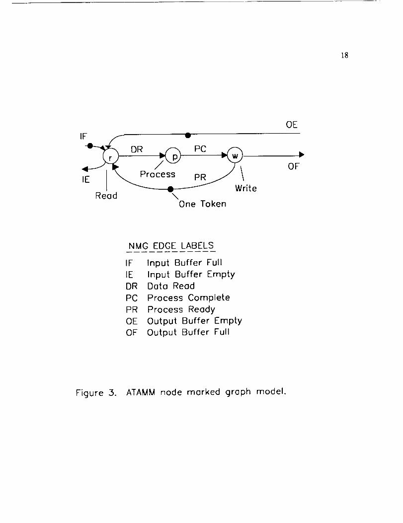
The nodemarkedgraph(NMG) is a Petri Net representationof the

performanceof analgorithmoperationby a functionalunit. Threeprimary activities,

readingof input datafrom global memory,processingof input data to computeoutput

data,and writing of outputdata to global memory,are representedas transitions

(vertices)in the NMG. Dataandcontrol flow pathsare representedas places(edges),

andthe presenceof signalsis notatedby tokensmarkingappropriateedges. The

conditionsfor firing theprocessandwrite transitionsof the NMG areasdefinedfor a

generalPetri Net, while thereadtransitionhasone additionalcondition for firing. In

addition to havinga tokenpresentoneachincoming signaledge,a functionalunit

mustbe availablein a queueof availablefunctionalunits for assignmentto the

algorithmoperationbeforethe readnodecan fire. Onceassigned,the functionalunit

is usedto implementtheread,process,andwrite operationsbeforebeing returnedto a

queueof availablefunctionalunits. The initial markingfor an NMG consistsof a

singletoken in theProcessReadyplace. The NMG model is shownin Figure3.

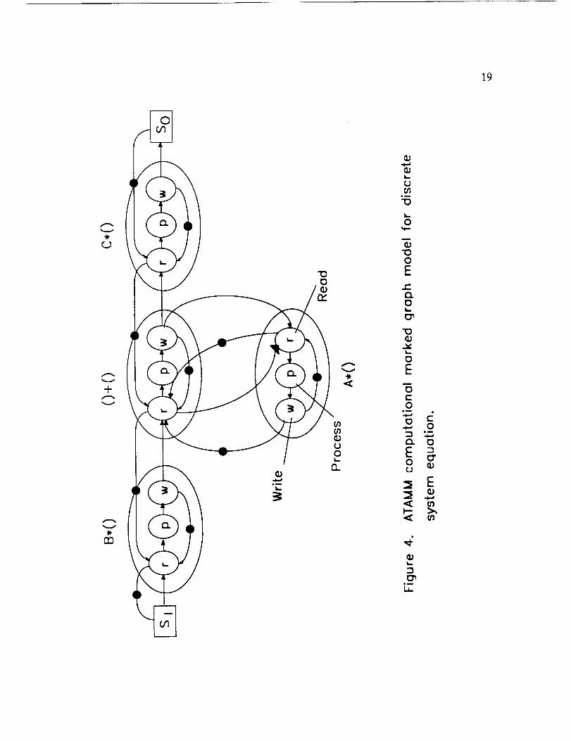
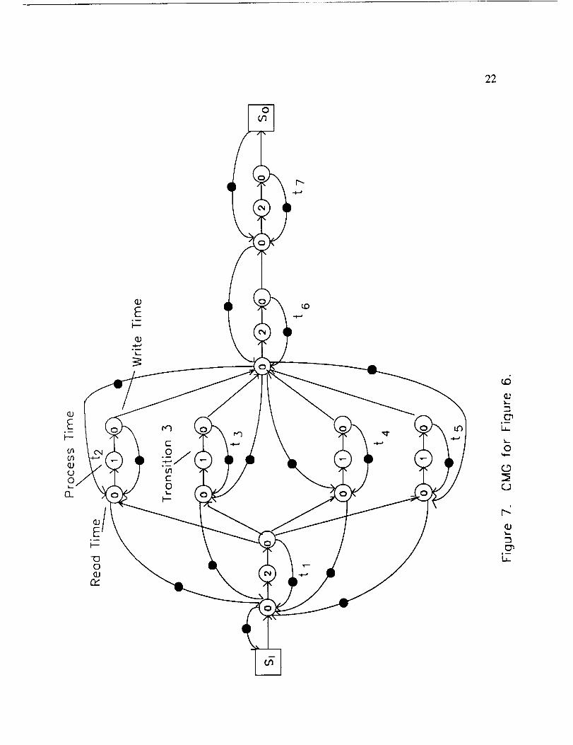
A computationalmarkedgraph(CMG) is constructedfrom the AMG and the

NMG by the following rules:

1) Sourceand sink nodesin the algorithmmarkedgraph

arerepresentedby sourceandsink nodesin the

CMG.

2) Nodescorrespondingto algorithmoperationsin the

algorithmmarkedgraphare representedby NMGs in

the CMG.

3) Edgesin the algorithmmarkedgrapharerepresented

by edgepairs, oneforward directedfor dataflow

and one backwarddirectedfor control flow, in the

CMG.

A forward directededgegoesfrom a predecessorwrite transitionto a successor

reador sink transition. Forwardedgesarealso shownaspart of the NMG in Figure2

wherethey arelabeledOF andIF edgesof the predecessorand successortransitions

respectively. A backwarddirectededgegoesfrom a successorreadtransitionto a

predecessorreador sourcetransition. Backwardedgesarealsoshownaspart of the

NMG wherethey are labeledOE andIE edgesof predecessorand successor

transitionsrespectively. The initial markingfor the edgepair consistsof a single

token in the forward directedplaceif dataareavailable,or a single token in the

backwarddirectedplaceif dataarenot available. In order to illustrate the

constructionof a computationalmarkedgraph,the CMG correspondingto the

algorithmmarkedgraphof Figure 1 is shownin Figure4.

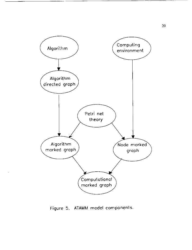
The completeATAMM modelconsistsof thealgorithmmarkedgraph,the

nodemarkedgraph,and thecomputationalmarkedgraph. A pictorial displayof the

componentsof the ATAMM modelareshownin Figure 5.

9

Graphexecutionbasedon the ATAMM rules hasseveralusefuland important

properties[5]. Executionis live, reachable,safe,deadlock-free,andconsistent[6].

Livenessindicatesthat all transitionsin the CMG are firable from the initial marking,

whereasreachabilityensuresthat CMG will generateanoutput for eachinput.

Safenessguaranteesthat outputof analgorithmoperationwill not beoverwritten

beforeit is picked up by a successoralgorithmoperationor sink. This propertyis a

result of includingbackwardcontrol placesin the CMG and is necessaryfor safe

periodic operation. The necessaryand sufficient condition for avoidanceof deadlock

in the graphplay is to ensurethat onceassigned,a functionalunit always is able to

completeexecutionof analgorithmoperation. A computationcannot enterdeadlock

becauseno readtransitionis executedunlessthe outputedgesof thecorresponding

NMG areempty anda functionalunit is available. The consistencypropertyimplies

that computationsarerepeatedperiodically wheninput areappliedperiodically.

2.2 Time Performance

In this section,thetime performanceof algorithmsimplementedin data flow

architecturesaccordingto the ATAMM rulesis investigated.First, performance

measuresfor computingspeedand throughputaredefined. It is shownthat the

ATAMM model is usefulfor analytically calculatingboundsfor thesemeasures.

Then,graphplay is describedandusedto determineresourcerequirementsnecessary

to achievea specifiedtime performance. Finally, theATAMM performanceplaneis

defined. This diagramdisplayspossibleoperatingstrategieswith resource

10

requirementsasa parameter. Using this display,a systemoperatoris able to specify

quantitativelysystemtime performance.

2.2.1. PerformanceMeasures

Two measuresof time performance,TBIO andTBO, aredefinedin this

section. The performancemeasureTBIO (time betweeninput andoutput) is the

elapsedcomputingtime betweenanalgorithm input andthe correspondingalgorithm

output. Therefore,TBIO is an indicatorof computingspeed. It is shownin [7] that

the algorithm imposed lower bound for TBIO, denoted ZBIOLa, is given by the sum of

transition times for nodes contained in the longest directed path from the input source

to the output sink in the AMG.

The performance measure TBO (time between outputs) is the elapsed

computing time between successive algorithm outputs when the AMG is operating

periodically at steady-state. Therefore, the inverse of TBO is an indicator of

throughput frequency. It is shown in [7] that the algorithm imposed lower bound for

TBO is given by the largest time per token of all directed circuits in the CMG. A

second bound on TBO is imposed by the availability of resources. It is shown in [6]

that the resource imposed lower bound for TBO is TCE/R where TCE (total

computing time) is the sum of transition times for all nodes in the AMG and R is the

number of available functional units. The lower bound for TBO, denoted TBOLB, is

the greater of the algorithm bound and the resource bound.

11

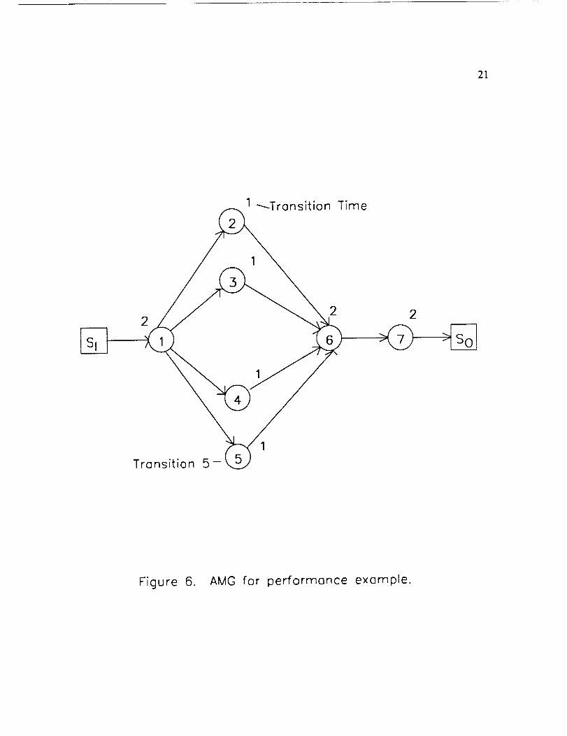
To illustrate the calculation of these performance bounds, consider as an

example the AMG shown in Figure 6 and the corresponding CMG shown in Figure 7.

The AMG contains four directed paths from the input source to the output sink. These

paths, identified by included transitions, are (1, 2, 6, 7), (1, 3, 6, 7), (1, 4, 6, 7) and (1,

5, 6, 7). The sum of transition times of nodes in each path is 7 so that TBIOLB = 7.

The largest time per token of any directed circuit in the CMG is 2. There are several

directed circuits which yield this result; one such directed circuit is the circuit

containing the read, process and write transitions of node 6 and the read transition of

node 7. Therefore, TBOLB = 2.

2.2.2 Graph Play and Resource Requirements

Two diagrams which display graph play and are useful for determining the

number of resources needed to achieve specified performance measures are defined

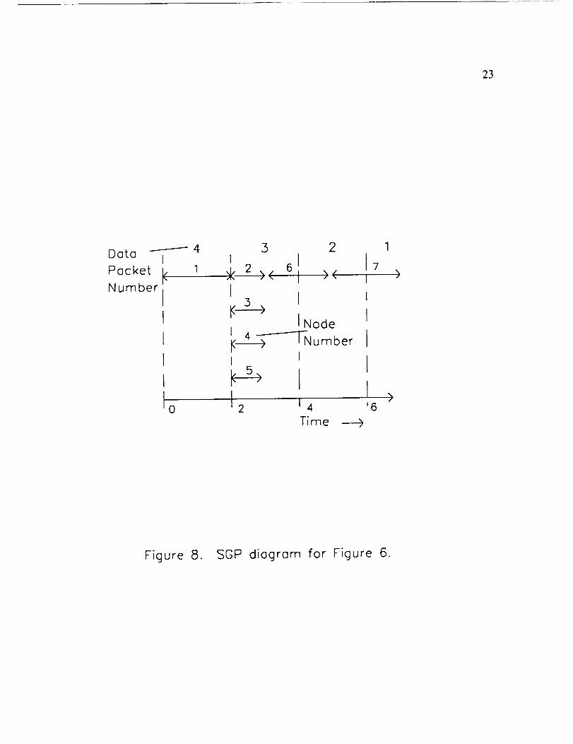
next. The SGP (single graph play) diagram is a diagram which displays the execution

of each node of the AMG as a function of time. The diagram is constructed for a

single input data packet under the assumption that unlimited resources are available to

play the graph. Node activity is denoted by a solid line and the symbols (<, >) are

used to indicate the beginning and end of execution. When several nodes are active at

the same time, lines indicating node activity are stacked vertically so that computing

concurrency is apparent. The SGP diagram for the AMG of Figure 6 is shown in

Figure 8.

12

Theresourcerequirementsto executea singledatapacketareobtainedby

counting the numberof activenodesduringeachtime interval in the SGPdiagram.

The peakresourcerequirementis denotedby Rmmand representsthe minimum number

of resourcesnecessaryto achieveoperationat TBIO = TBIOLa. For the AMG in

Figure 6, R_,,= 4 is the minimum numberof resourcesnecessaryto executethe graph

with TBIO = TBIOLB = 7.

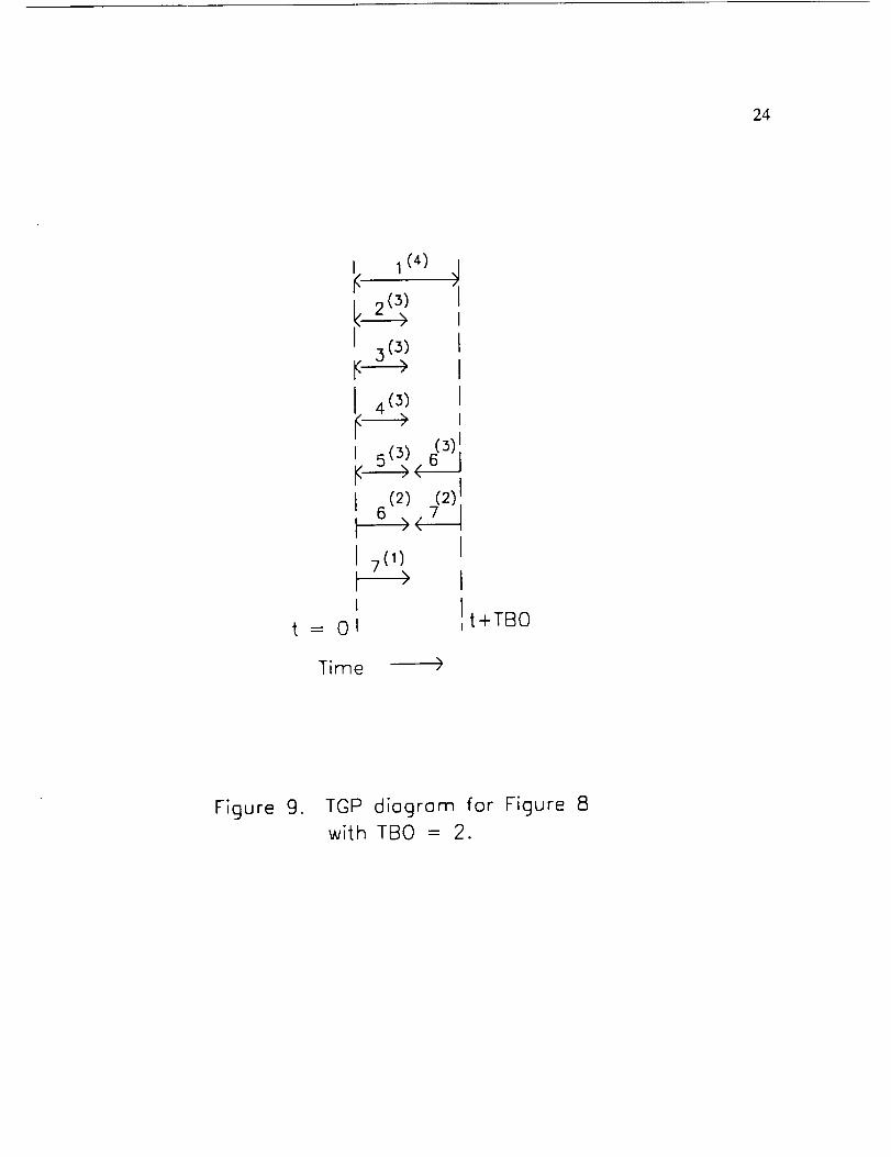
The TGP (total graph play) diagram is a diagram which displays the execution

of each graph node when the graph is operating periodically in steady-state with

period TBO. As with SGP, the diagram is constructed under the assumption that

unlimited resources are available to play the graph, and a different diagram results for

each value of TBO. The TGP diagram is drawn using information from SGP. SGP is

divided into segments of width TBO, and these segments are overlaid to form TGP.

Each segment from SGP represents a new input data packet. Data packets are

numbered sequentially so that the packet numbered i+l is the data packet which is

input to the graph TBO time units after the packet numbered i. To illustrate the

construction of this diagram, TGP for the AMG of Figure 6 is shown in Figure 9.

The resource requirements to execute multiple data packets injected with period

TBO are obtained by counting the number of active nodes during each time interval in

the TGP diagram. The peak resource requirement necessary to execute the graph

periodically with period greater than or equal to TBO is denoted by Rm,,. P_, is

determined by finding the largest resource requirement in all TGP diagrams drawn for

injection intervals greater than or equal to TBO. For example, the TGP diagram

13

drawn for TBO = TBOLB = 2 shown in Figure 9 indicates that a minimum of 7

resources is required. If this same TGP diagram is drawn for all values of TBO > 2,

it can be shown that the required number of resources remains less than 7. Therefore,

R_,_ to achieve TBO = 2 for the AMG shown in Figure 6 is equal to 7.

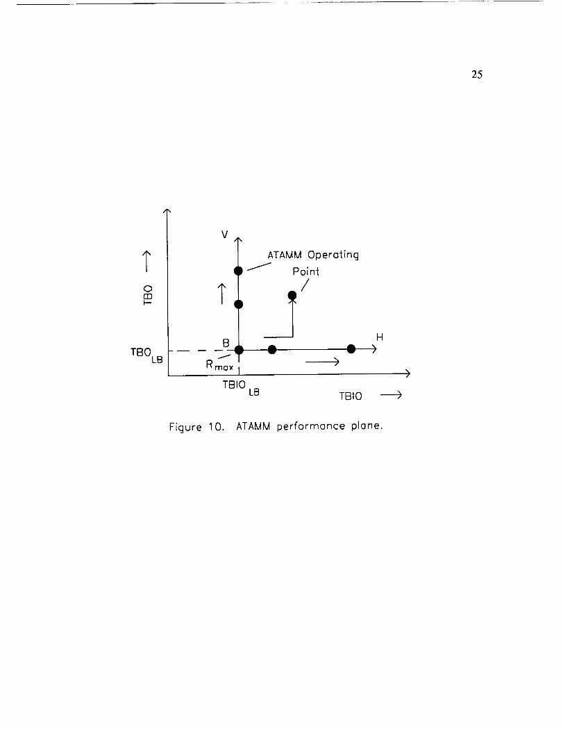
2.2.3. ATAMM Performance Plane

For a given algorithm decomposition, the parameters TBIO, TBO and R define

an operating point for ATAMM. The display of all operating points on a graph of

TBO versus TBIO with R indicated as a parameter is called the ATAMM performance

plane. The ATAMM performance plane, illustrated in Figure 10, is extremely useful

for selecting system operating strategies. The use of this diagram is described in this

section.

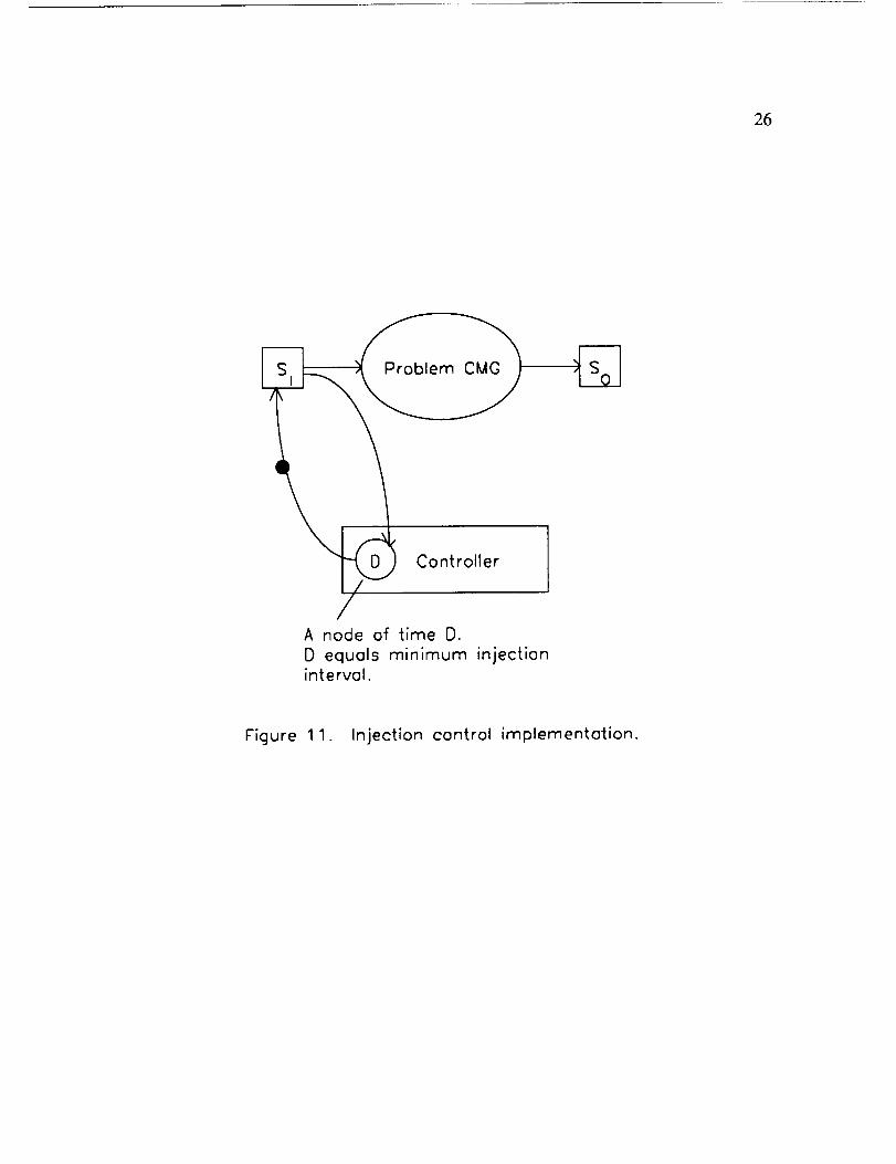
The best system performance is achieved by operating at point B where TBIO

= TBIOLB and TBO = TBOLB. The resource requirement associated with this operating

point is the value of R_,x computed from the TGP diagram drawn for TBIOLB and

TBOLB. Operation at point B is obtained by the use of injection control as shown in

Figure 11. Injection control is a control procedure which limits the maximum rate at

which new input data packets can be injected. When presented with continuously

available input data packets, the natural behavior of a data flow architecture results in

operation where data packets are accepted as rapidly as available resources and the

input transition permit. This leads to operation at a steady-state operating point where

TBO = TBOtB but TBIO > TBIOt.B. This occurs because the pipeline from input to

14

outputbecomescongestedwith extradatapacketswhich must wait for free resources

to beprocessed.Injection control eliminatesdatapacketcongestionandthus preserves

operationat TBIOLB.

When therearenot sufficient resourcesto operateat point B, the operating

point mustbe shifted to a new locationhavinga smallerresourcerequirement. Using

injection control procedures,it is possibleto shift theoperatingpoint vertically along

line B-V. This strategypreservesTBIO while degradingthroughputperformance.

Sucha strategyis usefulfor real-timecontrol and signalprocessingapplicationswhere

maintaininghigh computingspeedis very important. Operatingpoints on line B-V for

lower resourcerequirementsarecalculatedfrom the TGP diagramby increasingTBO

until the numberof activenodesin any time interval decreasesby onefrom the

previousoperatingpoint. Theseoperatingpoints are implementedby adjustingthe

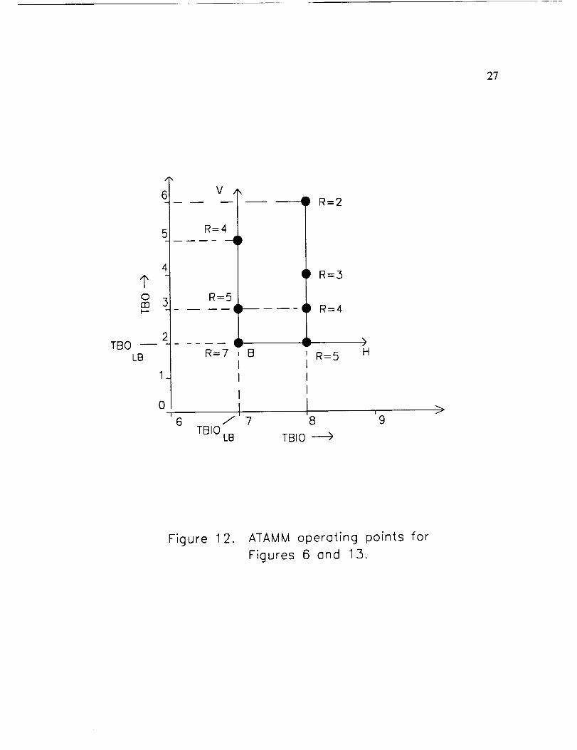
minimum input injection control interval. As anexample,considerthe AMG shown

in Figure 6. Operationat TBIO = 7 andTBO = 2 requires7 resources.By increasing

TBO to 3, thenumberof requiredresourcesdecreasesto 5. This canbe observedby

increasingthevalue of TBO in the TGP diagramof Figure 9 until the numberof

concurrentlyactivenodesdecreases.IncreasingTBO to 5 further reducesthe resource

requirementto 4 resources.Theseoperatingpoints aredisplayedin the ATAMM

performanceplaneasshownin Figure 12.

It is alsopossibleto shift the operatingpoint horizontallyalong the line B-H to

reduceresourcerequirements.This strategypreservesTBO while degrading

computingspeedperformance.Sucha strategyis useful for numbercrunching

15

applicationswheremaintainingthroughputis important. Operatingpoints on line B-H

for lower resourcerequirementsareobtainedby addingcontrol edgesto the original

AMG. A control edgeis an AMG placewhich imposesa precedencerelation among

two transitions,but doesnot imply datadependency.Whensuchanedgeis addedto

anAMG sothat the longestdirectedpath from the input sourceto the output sink is

increased,theresultingnew graphhasan increasedTBIO valuebut still describesthe

samealgorithm.

The additionof a control edgecancreatenew directedcircuits having

increasedtime per tokenvaluesso thatTBO is alsoincreased.This potential problem

is avoidedby addingdummynodesto the AMG. A dummynodeis anAMG

transitionwhich implementsan identity operationandrequireszerocomputationtime.

The dummynodeservesasa buffer to provideadditionalstoragefor the outputdata

of a graphnode. Implementationof a dummynodeis a memoryoperationandthus

doesnot requirea resource. Using the dummynode,it is possibleto increasethe

tokencount on circuits formedby addingcontrol edges,thuspreservingthe valueof

TBO in theoriginal graph. Controledgesanddummynodesalsocan beusedto

improveperformanceboundsand to balanceresourcerequirements.Operatingpoint

designusingcontrol edgesanddummy nodesis explainedin moredetail in [8].

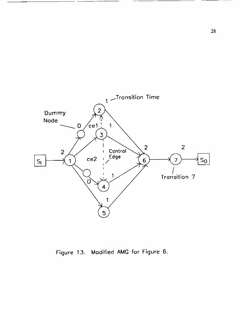
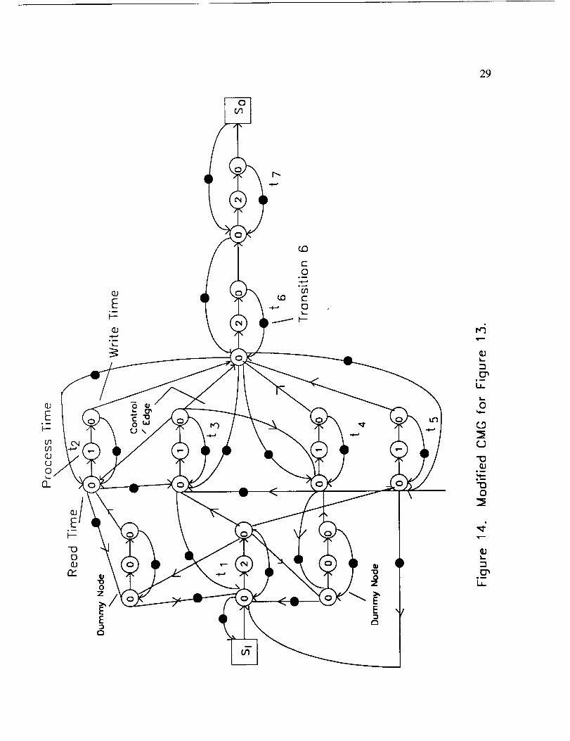
To illustrate shifting the operating point horizontally, consider again the AMG

shown in Figure 6. Adding a control edge directed from node 3 to node 4 creates a

new directed path from input source to output sink which contains nodes (1, 3, 4, 6,

7). Therefore, TBIOLB for the new graph is equal to 8. However, the control edge

16

alsocreatesa new directedcircuit containingthe read,processand write transitionsof

nodes1 and 3, andthe readtransitionof node4.

tokenvalueof 3 sothat TBOLBis increasedto 3.

This directedcircuit hasa time per

The time per tokenvalue of this

circuit is reducedby addinga dummynodeto theedgedirectedfrom node 1 to node

4. The new AMG andthe correspondingCMG areshownin Figures13 and 14,

respectively. A secondcontrol edgeanddummy nodearealsoaddedin Figure 13 for

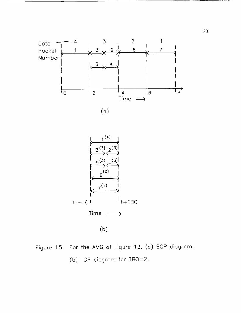
thepurposeof reducingthe peakresourcerequirement. The SGPdiagramandthe

TGP diagramfor TBO = 2 areshownin Figures 15. The new operatingpoint having

TBIO = 8, TBO = 2, and R = 5 is shownon the performanceplanediagram in Figure

12. Also shownareadditionaloperatingpoints onthe constantTBIO = 8 line which

are implementedby injectioncontrol asdescribedpreviously.

17

cj

J_

-_ C_C_

C_

o--

"0

0

c-

C_

"+O

O 0

E _O"

E __c E

0_

LL

18

IF S •

,_ _ ProcessP_JJ_iteRead \

One Token

OE

NMG EDGE LABELS

IF Input Buffer Full

IE Input Buffer Empty

DR Data Read

PC Process Complete

PR Process Ready

OE Output Buffer Empty

OF Output Buffer Full

Figure 3. ATAMM node marked graph model.

19

(J

÷

"00

QJ

(J00

Q_

"0

0

nO0

E

Cl.0X.

O_

nO

0c--0

O"0cJ

oI

Lu.

20

Petri net

theory

Algorithm mc

marked graph graph

putotional

marked graph

Figure 5. A-rAMM model components.

2]

1 _Transition Time

2 2

2

Transition 5-

Figure 6. AMG for performance example.

22

c_

_Jlira

C_

Ii

L.

o_D

cj

0_II

LL

23

_4Data I

Packet _ INumber

0

5 2l I_<-_->< 61 ><I

INode

.__>-------T-N u m b e r

I I

2 14

Time

II16

Figure 8. SOP diagram for Figure 6.

24

III

=01

1 (4)

I

I

L (3) j3)!

1 6 (2) 7_I >

7<_)> II

It+TBOI

Time _->

Figure 9. TGP diagram for Figure 8with TBO = 2.

25

0mk-

TBOLB

V

T

B Ii

J

R m13×

TBIO

ATAMM Operating

/ Point

/

Iw 'Iv

H

i,

LB TBIO

Figure 10. ATAMM performance plane.

26

Controller

A node of time O.

D equols minimum injectionintervol.

Figure 11. Injection control implementation.

2?

I'003p-

TBOLB

/

6

5

4

0

v

R=4

R=5I

lib

Iv

R=7

6TBIO

B

I R=2

II R=3

D R=4

R=5

I

IJ ?

LB

\

/

H

I

9>

Figure 1 2. ATAMM operoting points for

Figures 6 end 13.

28

1 /Transition Time

Dummy

Node_D

2

I, Control

ce2 ,/EdgeI

I

I

2 2

/Transition 7

Figure 13. Modified AMG for Figure 6.

E

u1oi

U0

EL

°/E

p--

"00

o2

E

Q

E°--

b--

°--

C0

t-

O

E

0

29

I-

L:.

0

"0

o--

noo

m--

LJ-

3O

Data I

Packet I¢Number

II

IIo

5

, $

Ii II12

2 1I I6 .. 7

4 16 8>Time ------>

(a)

t 1 (4) )l

I 5(3)4(3) I

(2)

7(_)

t=OI

I

I

I t+TBO

Time _->

(b)

Figure 15. For the AMG of Figure 13, (a) SGP diagram.

(b) TGP diagram for-rBO=2.

CHAPTER THREE

ATAMM ENHANCEMENTS

3.0 Introduction

In this chapter, enhancements to ATAMM developed for the ADM system are

presented. First, a method to control the time performance of the system based on

knowledge of the number of available processors is presented in Section 3.1. This

allows a user to specify system performance using the ATAMM performance plane

information given in Chapter 1. Then, new strategies for achieving fault tolerance in

the ADM system are described in Section 3.2. Included is the development of a

procedure for implementing triple mode redundancy (TMR) and a methodology for

dealing with processor failure during self test.

3.1. Real-Time Control Strategy

Included in AMOS for the ADM is the capability for on-line real-time control

of the system time performance. The ATAMM performance plane described in the

previous chapter displays all possible operating points, with the resource requirement

necessary to achieve the operating point shown as a parameter. A set of actual

operating points is selected by the user by identifying one operating point for each

resource number, R through 1. Each such point specifies the system time

performance, that is TBIO and TBO, for a particular number of available resources.

31

32

The setof actualoperatingpoints selectedin this way is compiledin a tablecalled the

operatingpoint table. The operatingpoint tableforms thecontrol law for

implementingthe real-timefeedbackcontrol strategyfor ADM. The calculationof

performanceboundsandconstructionof the SGP,TGP andperformanceplane

diagramshasbeenautomatedin a softwarepackagecalledDesignTool. The software

is beingdevelopedto operateon IBM PC/386compatiblesin theMicrosoft Windows

environment.

AMOS is designedto monitor continuouslythenumberof availablefunctional

units. At any instant,the numberof availableresourcesis usedto identify an

operatingpoint throughthe operatingpoint table. If thenumberof resourceschanges,

thena correspondingnew operatingpoint is identified. Systemoperationat the new

operatingpoint is achievedby adjustingtheinjection control time interval, and by

modification of the AMG throughtheaddition or deletionof control edgesand

dummynodes.

In the ADM system,the operatingsystemcountsthe numberof functionalunits

availableandcommunicatesthis numberto the IBM PC/386wherethe operatingpoint

tableis stored. Using a simpletable look-upprocedure,an operatingpoint is

identified and the graphstructureand injectionrate necessaryto realizethis operation

arespecified. This information is communicatedbackto the operatingsystemwhere

the graphstructureis changedand theinput rateadjusted. Therefore,theentire

feedbackcontrol processis integratedwith the ATAMM operatingsystem. The

control methodologyis shownin Figure 16.

33

3.2 Fault TolerantStrategies

The presentsectionis intendedto summarizethe Fault-TolerantStrategiesused

to enhancethe ATAMM strategy. The sectionis divided into two subsections:TMR

Implementationand FaultDetection& Recovery.

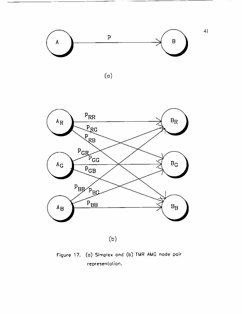
The TMR implementationin ATAMM is performedat the graphlevel. The

transformationof a graphto incorporatetheTMR strategyis explainedin detail. Fault

detectionandrecoveryareoutlinedin the last subsection.

3.2.1 TMR Implementation

TMR (Triple Modular Redundancy)is oneof manyFault-Detection-and-

Correctiontechniquesthatcanbe appliedin thedesignof a reliablecomputingsystem.

The philosophybehindTMR is to triplicate a givenwork or task to detectand correct

faults. The detectionis basedon the comparisonof the resultsof the multiple

outcomesor outputsof the triplicatedtask. Thecorrectionof thefault is

accomplishedby selectingone out of the threeoutputsasthe correctone. If thereis

anerror in anyof the threesets,the othertwo will be identical, hencethe latterare

assumedto becorrect. This schemeis usedto detectup to two faults but it canonly

correctone.

The implementationof TMR in ATAMM is achieved at the graph level. A

graph without the application of TMR is said to be a simplex graph. A simplex graph

is any normal graph defined to be executed under the rules of ATAMM. A TMR

graph is a graph that implements the TMR strategy in all of its nodes. A TMR graph

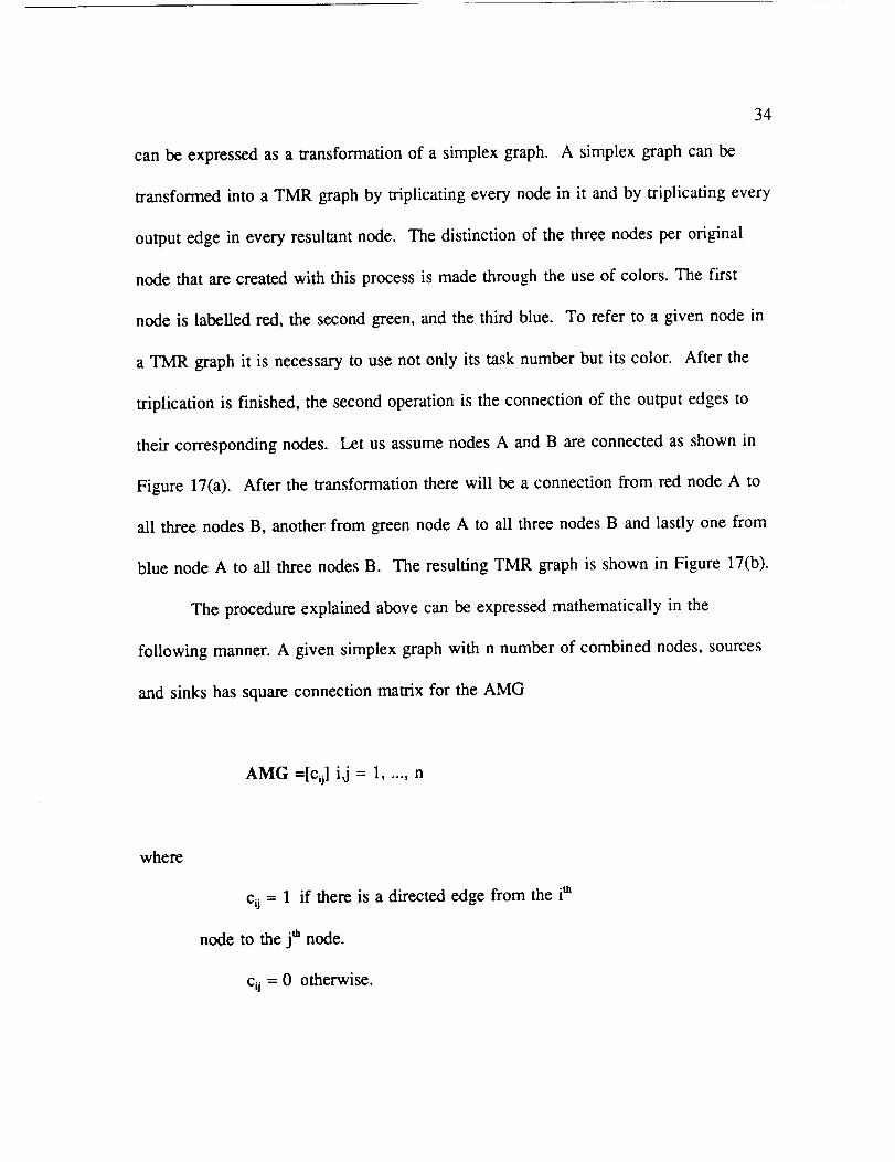
34

canbe expressedasa transformationof a simplexgraph. A simplexgraphcanbe

transformedinto a TMR graphby triplicating everynodein it and by triplicating every

output edge in every resultant node. The distinction of the three nodes per original

node that are created with this process is made through the use of colors. The first

node is labelled red, the second green, and the third blue. To refer to a given node in

a TMR graph it is necessary to use not only its task number but its color. After the

triplication is finished, the second operation is the connection of the output edges to

their corresponding nodes. Let us assume nodes A and B are connected as shown in

Figure 17(a). After the transformation there will be a connection from red node A to

all three nodes B, another from green node A to all three nodes B and lastly one from

blue node A to all three nodes B. The resulting TMR graph is shown in Figure 17(b).

The procedure explained above can be expressed mathematically in the

following manner. A given simplex graph with n number of combined nodes, sources

and sinks has square connection matrix for the AMG

AMG =[ci_ i,j = 1..... n

where

c U = 1 if there is a directed edge from the ith

node to the jtb node.

c,j = 0 otherwise.

A vector of m square matrices is

35

[MI M2 M3 ... Mm]

In general, the connection matrix for a CMG is defined as the sum of two

matrices, EC and IC. These two matrices are: the external connection of the nodes of

the AMG and the internal connection of the AMG. These two matrices can only be

defined in terms of the NMG. The connection matrix of the NMG that is being used

in the definition of ATAMM can now be defined. The NMG is composed of three

transitions, namely: read, process and write. The connection matrix that defines the

internal connection of these transitions is

NMG=[c U]i,j= 1 ..... 3

where

cij = 1 for the pairs (i, j) = (1, 2), (2, 3), (3, 1),

cij = 0 otherwise.

where 1 corresponds to the read transition, 2 to the process transition and 3 to the

write transition.

Once the NMG is given, the external connection matrix EC can be defined. If

nodes A has a directed edge to node B in an AMG, then the write transition of node A

hasa directededgeto thereadtransitionof nodeB. Also thereis a directededge

from the readtransitionof nodeB to thereadtransitionof nodeA. Therefore,the

externalconnectionmatrix EC is definedas

36

EC = [0 0 I] r [AMG] [I 0 0] + [I 0 0]T[AMG]T[I 0 0]

which is a 3n x 3n matrix where n is the number of nodes, sinks, and sources in the

AMG. I is a n x n identity matrix and 0 is a n x n zero matrix.

The internal connection matrix IC is defined as follows

IC = [I 0 0]T[I][0 I 0] +

[0 1 0]T[I][0 0 I] +

[0 0 IIT[I][I 0 0]

then

CMG = EC + IC

or

CMG =

F"

I AMG T

I o[ AMG+Ik

I

0

0

0

I

0

37

where CMG is a 3n x 3n connection matrix and n is the number of nodes, sinks, and

sources in the AMG.

The connection matrix AMG3 of a TMR graph is expressed in terms of the

connection matrix AMG of a simplex graph. This is

AMG3 = [I I I] T AMG [I I I]

where AMG3 is a 3n x 3n connection matrix.

graph is

The CMG connection matrix of a TMR

CMG =

F- -1

I AMG3 "r I 0 I

] 0 0 I ]

] AMG3+I 0 0 IL J

Each colored node (red, green and blue) reads three sets of the original simplex

data sets. Each of these data sets comes from a colored node from the predecessor

nodes. The first operation that a node has to execute is the comparison of the three

data sets. This comparison is performed by a unit called voter. The voter compares

all data sets and determines if there is any error on any of the sets. The output of the

voter is divided in two parts. The first part is a data set to be used in the task of the

node. The second part corresponds to an error report. There are three possible

outcomes in the error report, they are: there is no error in the data sets; there is a

38

recoverableerror in the datasets;andthereis a fatal error. The first refersto the case

wherethere is no differenceamongall threedatasets. Any dataset is thenusedas

input to the node. The second error refers to the case where there was one set in

disagreement with the other two. Any data set of the two in agreement is then used as

the input set to the node. The color of the node that produced the erroneous data can

be part of the error output. The third error refers to the case where there were not two

data sets in agreement. That is, there is more than one error. In this instance any data

set can be used since there is no way to determine which is in error or which is

correct. This is a fatal error since this error propagates erroneous data throughout the

graph. This error should flag an exemption to the operating system to take a

corrective action.

3.2.2 Fault Detection and Recovery

Fault detection in ATAMM can be implemented at the graph manager [3] level.

The graph manager is the part of the implementation of ATAMM that runs the graph.

It scans the graph seeking enabled nodes and assigns resources that execute them. The

graph manager assigns a resource to a computing node. The resource executes the

given operation. After this resource has finished and delivered the output data to the

appropriate data edges, the resource can be tested before it returns to be available to

the system. This can be a self-test of the resource. The result of this test is then

passed to the graph manager. Based on the test result, a decision is made whether the

resource is able to continue being used by the system or has to be discarded from it.

39

Recoveryis fulfilled by discardingthe resourcethat reportedanerror during its

test. The resourceis not allowedbackinto the systemby not beenavailablefor

assignmentby the graphmanager. It is clear that thetype of fault that canbehandled

is the onethat canbedetectedby the resourceitself. This type of fault includesfaults

in the subsystemsof the resourcesthat do not directly intervenein the executionof

instructions,e.g.,ALU operations,I/O operations,etc. This summarizesthe fault

detectionandrecoveryof ATAMM.

4O

AOM

AMOS MULTICOMPUTER

ARCHITECTURE

Graph

Cha racterization

&

Injection Rotes IBM PC/386

Operating Point

Table

_"_ Number of

esources

On-Line Operations

Off-Line Performance Design

ATAMM Support

Tools

Figure 16. Control strategy for ADM system.

P41

(o)

PRRAR BR

P

GGA G BG

PGB

P

AB PBB BB

(b)

Figure 17. (o) Simplex and (b) TMR AMG node pair

representation.

CHAPTER FOUR

ADM IMPLEMENTATION OF ATAMM

4.0 Introduction

In this chapter, the adaptation of the ATAMM model to the ADM system is

described. The architecture of the ADM system is discussed in Section 4.1. In

Section 4.2, the major components of the ATAMM Multicomputer Operating System

(AMOS) are identified and AMOS operations are explained using a state diagram

description. Then the software of 1553B and IBM PC/386 are described in Section

4.3 for input/output communication and real-time control.

4.1. ADM Architecture

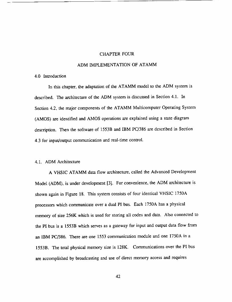
A VHSIC ATAMM data flow architecture, called the Advanced Development

Model (ADM), is under development [3]. For convenience, the ADM architecture is

shown again in Figure 18. This system consists of four identical VHSIC 1750A

processors which communicate over a dual PI bus. Each 1750A has a physical

memory of size 256K which is used for storing all codes and data. Also connected to

the PI bus is a 1553B which serves as a gateway for input and output data flow from

an IBM PC/386. There are one 1553 communication module and one 1750A in a

1553B. The total physical memory size is 128K. Communications over the PI bus

are accomplished by broadcasting and use of direct memory access and requires

42

43

exclusivecontrol over a singlePI bussemaphore.A processoror 1553Bmust grab

the PI bus semaphorebeforecommunicatingover thePI bus. All processorsalso

communicateoveran IEEE-488busto a Microvax computerwhich is usedto

downloadapplicationprogramsand files for debuggingactivities. The 1553Bmodule

is connectedto the IBM PC/386by a single line communicationlink. Dataare

transferredbetweenthe 1553Bmoduleandthe IBM PC/386by synchronous

communications.It is possibleto perform logical operationsin 1553Band

communicationsover thePI busandcommunicationlink concurrently. In addition to

input and output,the communicationlink is usedfor fault injection, fault recovery,

modification of the algorithmgraphin real-time,andpassinginformationback to IBM

PC/386for testingpurposes.The 1553Bactsasa sourceand sink for the algorithm

markedgraphandthus is capableof controlling the input injection rateto the 1750A

processorsandcollecting output from the PI bus.

4.2 AMOS Description

The ATAMM MulticomputerOperatingSystem(AMOS) is the operating

systemof the ADM hardwareandits operationis baseduponATAMM rules. First,

fundamentalprinciplesof AMOS aredescribed.Second,a detaileddescriptionof

AMOS datastructuresarepresented.Third, anexampleis usedto illustratethe

operationsof the operatingsystem. Finally, the operationsperformedby a functional

unit areelaborated.

44

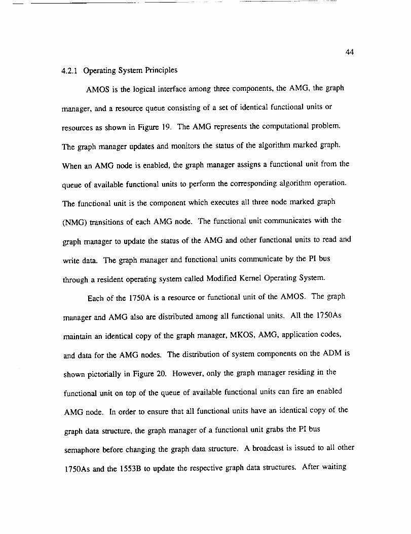
4.2.1 OperatingSystemPrinciples

AMOS is thelogical interfaceamongthreecomponents,the AMG, the graph

manager,and a resourcequeueconsisting of a set of identical functional units or

resources as shown in Figure 19. The AMG represents the computational problem.

The graph manager updates and monitors the status of the algorithm marked graph.

When an AMG node is enabled, the graph manager assigns a functional unit from the

queue of available functional units to perform the corresponding algorithm operation.

The functional unit is the component which executes all three node marked graph

(NMG) transitions of each AMG node. The functional unit communicates with the

graph manager to update the status of the AMG and other functional units to read and

write data. The graph manager and functional units communicate by the PI bus

through a resident operating system called Modified Kernel Operating System.

Each of the 1750A is a resource or functional unit of the AMOS. The graph

manager and AMG also are distributed among all functional units. All the 1750As

maintain an identical copy of the graph manager, MKOS, AMG, application codes,

and data for the AMG nodes. The distribution of system components on the ADM is

shown pictorially in Figure 20. However, only the graph manager residing in the

functional unit on top of the queue of available functional units can fire an enabled

AMG node. In order to ensure that all functional units have an identical copy of the

graph data structure, the graph manager of a functional unit grabs the PI bus

semaphore before changing the graph data structure. A broadcast is issued to all other

1750As and the 1553B to update the respective graph data structures. After waiting

45

for a predeterminedtime interval to allow the updatingto complete,the functionalunit

releasesthe PI bus for othercommunication. This distribution of activities hasthe

advantageof increasingthenumberof functionalunits in the systemand at the same

time improving thepotential for achievinga higherdegreeof fault toleranceto

functionalunit failure.

The operationof a functionalunit is representedby thestatediagramshownin

Figure 21. Initially, all functionalunits awakein the statelabeledIdle. A functional

unit remainsin this stateuntil its identifier appearsat the top of the resourcequeue.

When this occurs,thefunctionalunit undergoesa statetransitionto the Examine

Graphstate. In this state,the functionalunit actively monitorsthe statusof the AMG

until an algorithmnodebecomesenabled. Whenanenabledalgorithmnodeis

identified, thefunctionalunit assignsitself to perform the algorithmoperation,grabs

the PI bus,andundergoesanotherstatetransitionto theExecutestate. During this

statetransition,the functionalunit identifier is removedfrom the top of the resource

queueand a buscommunicationF announcingthat analgorithmoperationhasbeen

initiated is broadcaston the bus. Then, the functionalunit releasesthe PI bus. The

functionalunit remainsin the Executestateuntil the algorithmoperationis complete.

At the completionof thealgorithmoperation,the functionalunit grabsthe PI bus

semaphoreandinitiatesa secondbuscommunicationD which includesa broadcastof

the algorithmoperationoutputdata to all other functionalunit global memories. At

this time thefunctionalunit againchangesstateto the Self Test stateandreleasesthe

PI bus. The Self Test statecorrespondsto a diagnosticcheckof the functionalunit.

After a successfulself test,the functionalunit returnsto the initial Idle state. This

statetransitionis accompaniedby a grabbingof thePI bussemaphore,a third bus

broadcastcommunicationR announcingthat the functionalunit identifier shouldbe

returnedto the bottom of theresourcequeue,anda releaseof PI bus. While in any

state,the functionalunit maybe interruptedto updateits graphdatastructuresand

resourcequeuesfollowing F, D, or R broadcastsfrom other functionalunits.

46

4.2.2 DataStructures

The datastructuresof AMOS consistof two arrays,BLOCKS and EDGES,

that hold all of the information regardingnodesandedgesof analgorithm marked

graph. Also, there is a table,PRIORITY, that holdstheprecedenceorderof the

nodesof the algorithmgraph. In addition, therearefour queues,QUEUE, WORK,

DIAG, andRECOV that hold informationaboutcurrent statusof functionalunits. The

QUEUE is a FIFO queueof availableandunassignedfunctionalunits,WORK is a

pool of assignedfunctionalunits, DIAG is a pool of functionalunits in a diagnostic

state,and RECOV is a pool of functionalunits to be recoveredby the system. In this

sectiona detaileddescriptionof thesedatastructuresarepresented.

Everyfunctionalunit (1750As)hasan instanceof AMOS. After everyF, D, or

R events,thegraphandresourcestructuresareupdatedby theindividual 1750As

separately.ThevariablesBLOCKS, EDGES,PRIORITY, QUEUE, andetc. are

definedasarrays. Although thesevariablesaredef'medas arrays,they are treatedas

47

linked lists, i.e., the linked list is implementedusingarray indices. The linked list

structurereflects the dynamicstructureinherentin this architecturemodel.

A block is a nodeof AMG. In TMR mode,it is a set of threecolored-nodes,

red, green,and blueand in SIMPLEX modea setof only onenode. Its primary useis

in TMR mode. FIRING is a global variablethat holdsthe identificationcode(ID) of

the block being fired. It is usedto ensurethat all of thecolored-nodesof the block

arefired before firing the next block. If thereis no block being fired, then it is set to

zero. MODE, a global variable,indicatesthemodeof operationandis initially set by

the userto SIMPLEX, 1,or TMR, 3. In TMR mode,whenthe numberof functional

unitsdrops to lessthan three,AMOS will changethevalue of MODE to SIMPLEX to

reflect the decreasein the numberof functioningresources.BLOCKS is anarrayof N

elementswith componentsBLOCKS[j], the rangeof j is from 0 to N, whereN

representsthe numberof nodesin the AMG graph. EDGESis an arrayof M elements

with componentsEDGES[k], therangeof k is from 0 to M, whereM representstotal

numberof edgesin the AMG graph. QUEUE, WORK, DIAG, and RECOV arearrays

of sizeequal to the maximumnumberof availablefunctional unitsat the start up.

Thesearraysaredescribedin the following paragraphs.

BLOCKS: BLOCKS[j] is an element of the array BLOCKS and holds all information

about a block. BLOCKS[J] consists of nine variables which are explained below.

FUNCTION_ID is an integer representing the task ID or a pointer pointing to the

application program. ID is a three element array which holds the identification code

of functional units assigned to the colored-nodes of the block. ID is used to keep track

48

of functionalunits for future recoverypurposes.BUSY_CTR is a counterthat holds

the numberof functionalunits working on the block. It is incrementedafter every

F-transitioncommandanddecrementedafter everyD-transitioncommand. Another

variable,DONE_CTRis a counterthat holdsthe numberof functionalunits released

from the block. It is usedto check if a block canbeenabled. It is setto zerowhen

the block is enabledandis incrementedby everyD-transition. ENABLE_CTR is a

counterthat holdsthe numberof enabledcolored-nodesthat havenot yet fired. When

theblock is firable theENABLE_C'I_ is setto the MODE of operation. It is

decrementedafter everycolored-nodeof a block is fired (F-transition). INPUTS is an

arrayof pointershavingcomponentsINPUTS[i], wheretherangeof i is from 0 to 2.

INPUTS[i] is the headerpointerpointing to a linked list of input (incomingdata)

edgesto the ith colored-node.Anothervariable,OUTPUTSis an arrayof pointers

havingcomponentsOUTPUTS[i], wherethe rangeof i is from 0 to 2. OUTPUTS[i]

is the headerpointer pointing to a linked list of output(outgoingdata)edges

originatingfrom the ith colored-node.(It implicitly representsall backwardcontrol

edgesfrom all successornodesto this node.) Figure22 is a pictorial representationof

thesetwo linked lists. IN_SUMMARY is an arrayof integerswith components

INSUMMARY[i], wherethe rangeof i is from 0 to 2. IN_SUMMARY[i] is a

summaryof INPUTS[i] and is an integerhavinga valueequal to the numberof input

edgesof the ith colored-nodewhenall havedataandis zerootherwise.

OUT_SUMMARY is anarrayof integerswith componentsOUT_SUMMARY[i],

wherethe rangeof i is from 0 to 2. OUT_SUMMARY[i] is a summaryof

49

OUTPUTS[i] and is an integerhavingvalueequal to the numberof outgoingedges

originating from the ith colored-nodewhenall areempty andis zerootherwise. A

block is enabledunder the following conditions:

1. DONE_CTR = MODE,

2. All IN_SUMMARY[i]s, i = 0..2,arenon-zero,and

3. All OUT_SUMMARY[i]s, i = 0..2, arenon-zero.

EDGES: EDGES[k] is an element of the array EDGES and holds all information

about an edge. EDGES[k] consists of eleven variables which are described in the

following. EDGE_QUEUE is a circular linked list that holds addresses of the memory

locations where the data are stored. The addresses are accessible to the INITIAL and

TERMINAL blocks to write and read data, respectively. For future recovery purposes

the length of the queue, L, is one more than the SEGMENTS or, number of Dummy

nodes plus two. Structure of each element of the EDGE_QUEUE consists of three

elements; a) LABEL is a pointer to the beginning of the data container, b) ID holds

the identification code of the functional unit which wrote the data into that data

container, and c) NEXT is a pointer to the next element of the EDGE_QUEUE.

SEGMENTS is an integer equal to the number of dummy nodes on the edge plus one.

It is used to check capacity of the EDGE_QUEUE of the edge. If SEGMENTS is

equal to ITEMS, then EDGE_QUEUE is full and no more data can be written into it.

ITEMS is a counter indicating the number of data items on the edge. The range of

ITEMS is from zero to SEGMENTS. It is incremented, by the INITIAL node, every

time new data are written on the edge. It is decremented, by the TERMINAL node,

50

every time OUTPUT_WIDTH becomeszero. INITIAL holds the block numberof the

origin of the edge. It is used to update the graph and can also be used to check the

integrity of the graph. TERMINAL holds the block number of the destination of the

edge. It is used to update the graph. EDGE_COLOR indicates the color of the

INITIAL node of the edge. It is also used to update the graph. The value of color is

identified as 1 for red, 2 for green, and 3 for blue. OUTPUT_WIDTH, a counter, is

set to MODE when its present value is zero and ITEMS is non-zero. It is

decremented by one for each F-transition of the TERMINAL block.

TERMINAL_PTR is a pointer to the element of the EDGE_QUEUE where the

TERMINAL node reads data. It is updated every time OUTPUTWIDTH becomes

zero. Updating TERMINAL_PTR means that it should be pointing to the next

element of the EDGE_QUEUE. Updating is performed by the TERMINAL node.

INITIAL_PTR is a pointer to the element of the EDGE_QUEUE where the INITIAL

node writes data. It is updated every time an output is written to the edge. Updating

INITIAL_PTR means that it should be pointing to the next element of the

EDGE_QUEUE. Updating is performed by the INITIAL node. NEXT_INPUT is a

pointer to the next edge which is an input edge to the TERMINAL block.

NEXT_OUTPUT is a pointer to the next edge which is an output edge of the INITIAL

block. NEXT_INPUT and NEXT_OUTPUT are used to examine all of the input and

output edges of a block, respectively.

QUEUE: QUEUE is a FIFO queue holding information about available and

unassigned functional units. Each element of the QUEUE is a record of three

51

componentsID, COLOR, andNEXT. ID holdsthe identificationcode of an available

functionalunit. COLOR is a variablecontainingthecolor of the colored-nodeof the

enabledblock that thefunctionalunit will process.COLORcarriesrelevant

informationonly whenit belongsto one of thetop MODE elementsof theQUEUE.

The COLOR valueis assignedaccordingto the positionof the functionalunit in the

top of the QUEUE; first red, secondgreen,andthird blue. NEXT holdsthe index of

the next elementof the QUEUE. It is usedto treatQUEUE asa linked list. If

NEXT is zero,then thereareno moreelementsin the list. The first elementof

QUEUE is usedasa dummyheadnodeof the linked list andto keep track of content

of thearray. Note that the COLORfield of thefirst elementholdsthe numberof

functionalunits in the array.

WORK, DIAG: WORK and DIAG have the same structure as QUEUE but are treated

differently. WORK is a pool holding identification codes of all functional units which

have been processing nodes. DIAG is a pool holding IDs of functional units which

are in a diagnostic state.

PRIORITY: It is an array holding block numbers. The position in the array

determines the block's priority. The block at the first element is the block with the

highest priority in the graph.

4.2.3 Example

This example is provided to give more insight to the data structures of AMOS.

Figure 23 is part of a graph considered for this example. In this example, the focus is

52

on the nodelabeledE and all of the changes regarding these nodes are depicted in the

following figures. The mode of operation is SIMPLEX. Figure 24 is a pictorial

representation of the data structure and contents of QUEUE, WORK, DIAG, EDGES,

and BLOCKS. The initial contents of EDGES[i], the range of i is from 0 to 3, are

shown in Figure 25. Figure 26 depicts the structure of EDGE_QUEUEs of all the

edges. Note that the edge from E to C has a dummy node and thus the length of its

EDGE_QUEUE is one more than other edges. The read and write pointers of the

edges are also shown in this figure. The initial contents of block E are shown in

Figure 27. When block E is enabled, the ENABLE_CTR is set to the MODE and

IN_SUMMARY is cleared as shown in Figure 28. The functional unit assigned to the

block E is transferred from the QUEUE to WORK and starts reading inputs to the

block E. After reading the input on the AE edge, ITEMS of AE edge is decremented

and the read pointer of the block E concerning this edge, E_Read, is advanced. The

NEXT_INPUT field of AE edge provides the block E with the information about next

input to the block as in Figure 29. After reading the input on the BE edge, ITEMS of

BE edge is decremented and the read pointer of the block E concerning this edge,

E_Read, is advanced. The NEXT_INPUT field of BE edge provides the block E with

the information about next input to the block. The value of that pointer for this graph

is now Nil indicating the end of reading process for the block E as shown in Figure

30. While processing the application program as described in Figure 31, there are no

changes in the data structure of block E. After writing to edge ED, ITEMS of ED

edge is incremented. The NEXT_OUTPUT field of ED edge provides the block E

53

with informationaboutnextoutputedgeof the block. Also the write pointerof the

ED edge,E_Write, is advancedso that theblock E can write to the newplacenext

time asshownin Figure 32. After writing to edgeEC, ITEMS of EC edgeis

incremented.Also thewrite pointerof the EC edge,E_Write, is advancedsothat the

block E canwrite to the new placenext time. The NEXT_OUTPUT field of EC edge

providestheblock E with informationaboutnextoutputedgeof the block. A pointer

with a valueof Nil indicatestheend of theprocess. At this point, the graphis

updatedbefore broadcastingasdescribedin Figure 33. After writing theoutputdata

and broadcastingtheupdatedgraph,thefunctionalunit migratesfrom the WORK to

DIAG to performa self test. Note that the DONE_CTRis setto the MODE of

operationas in Figure 34.

4.2.4 FunctionalUnit Operations

Every functionalunit hasan instanceof AMOS. Althoughevery functional

unit hasknowledgeof statusof otherprocessors,it actsasa standaloneentity. Every

functional unit goesthrougha sequenceof operationsas shownin Figure 35. These

operationstogetherform the statesof theresourcestatediagramof Figure21.

Implementationof AMOS is bestunderstoodby examiningtheseoperationsof

functionalunits.

Idle." When in Idle, the functionalunit examinesthe QUEUE continuously. First

QUEUE is checkedto determineif thereareat leastasmany functionalunits in the

QUEUE as theMODE of the systemby examiningQUEUE[0].ID. Second,QUEUE

54

is checkedto determineif QUEUE[i].ID is the sameasits own ID, wherethe rangeof

i is from 0 to MODE. If the self identification is successful,the searchis thenmade

for anenabledblock basedon priorities assignedto theblocks. An enabledblock is

detectedby examiningIN_SUMMARY[i], OUT_SUMMARY[i], andthe DONE_CTR.

The variablesIN_SUMMARY[i] andOUT_SUMMARY[i] are,in this state,assigned

propervaluesby examiningall input andoutputedgesof the block. This search

continuesuntil anenabledblock is found. Havinga block to execute,the functional

unit selectsa colored-node,basedon its position in the QUEUE,to fire. The global

variable FIRING is set to the ID of the block. After FIRING holdsa valid ID, the

functionalunit selectsthe appropriatecolored-nodeof that block to executeand

changesstateto On_Hold_Readstate.

On Hold Read: While in On_Hold_Read state, the functional unit is constantly trying

to get control of a communication channel. The reason being that the functional unit

must inform all other functional units before the execution of the AMG node begins.

Duration of this state depends on the traffic and communication channel protocol.

Update and Read: After establishing a communication link, the functional unit

conducts a second search for enablement of nodes with higher priorities than the

previously enabled nodes. Selecting a node with the highest priority, the functional

unit migrates from the QUEUE to the pool of working functional units(WORK). The

variable BUSY_CTR is incremented and ENABLE_CTR is decremented. It then

updates its copy of the graph and instructs all other processors and 1553B to do the

same. This broadcast is called a F event. The communication channel is then

55

released.Readingof input data begins after releasing the channel. After reading

every input, the variable OUTPUT_WIDTH of the corresponding edge is decremented.

If the current value of OUTPUT_WIDTH is zero, the pointer TERMINAL_PTR of

that edge is advanced and the variable ITEMS is decremented. In TMR mode, the

functional unit votes on the three sets of inputs and chooses the correct set for

processing.

Process: In this state, the functional unit executes the application program. To do so,

control is passed to the application program. Upon completion of the task, control is

passed back to AMOS. Duration of this state is the same as execution time of the

application program.

On Hold Write: To write the generated outputs, the functional unit has to get control

of a communication channel. Duration of this state depends on the traffic and

communication channel protocol.

Update And Write: After establishing a communication link, the functional unit

identification is removed from the WORK queue to the diagnostics queue (DIAG).

The DONE_CTR is incremented and the BUSY_CTR is decremented. In this state the

functional unit writes the output data to the memory locations associated with the

appropriate edge. The variable ITEMS of the corresponding edge is incremented and

the pointer INITIAL PTR of that edge is advanced. The functional unit updates its

copy of the graph and then broadcasts data and instruction to update graph structure in

other processors and 1553B. This broadcast is called a D event. If an error is

detected in the Read state, the color of the node and ID of the functional unit

56

responsiblefor theerror aresentalongwith the D event. The communicationchannel

is then released.

Test: In this statethefunctionalunit performsa self test. Uponcompletion,the

functionalunit requestsfor a channel. Durationof this statedependson the test

routine.

On Hold Uodate: To let the system know about its availability to undertake a task,

the functional unit needs to grab a communication channel.

Update: After establishing a communication link, the functional unit identification is

removed from the DIAG queue and placed in QUEUE, if the self test was successful.

Otherwise, it simply removes itself from the diagnostics queue. In any case, the

functional unit broadcasts the updated resource queues (this broadcast is called a R

event) and releases the communication channel.

4.3 1553B Software

Four major tasks are performed by the code of 1553B. First, communication

between 1553B and IBM PC/386 are controlled by the code of 1553B. Second, source

and sink for a computational problem are implemented in the 1553B. Third, all FDTs

(FDT stands for Fire, Data, Time) are received from 1750As and time tagged. The

format for the FDT is described in Figure 36. A binary coding is used and each FDT

is 8 words (128 bit) long. The meaning and size of binary codes of the FDT are also

described in the above figure. Fourth, the code of 1553B is used to control the time

57

betweensuccessiveinputs(TBI) to 1750As, to pass control words from the IBM

PC/386 to 1750As, and to pass back status information of 1750As to the IBM PC/386.

Both 1553B and IBM PC/386 have a transmit and a receive buffer. The

contents of the transmit buffer of the 1553B is written onto the receive buffer of the

IBM PC/386 periodically. Similarly, the content of the transmit buffer of the IBM

PC/386 is transmitted to the receive buffer of the 1553B at the same periodic rate.

The maximum size of the transmit and the receive buffers are 32 addresses where each

address points to a 32 word (each word is 16 bit long) data. The contents of the

transmit and the receive buffers are described in Figure 37. The transmit buffer of the

1553B and the receive buffer of the IBM PC/386 are divided in output buffer, FDT

buffer, status AMOS buffer, and status 1553 buffer. The first word of the output and

FDT buffers indicates that length of output data and the number of FDTs, respectively.

The size of the output and FDT buffers are specified during initialization depending on

the maximum requirement. The status AMOS buffer is a 32 word long buffer

indicating status of AMOS which is updated at every broadcast by 1750As. The

contents of the status 1553 buffer are an input flag, an output flag, a FDT flag, a

control flag, an error code, and an error flag. The error flag the and error code are

used to indicate overflow in either FDT or output queues in the 1553B. All other

flags are needed for handshaking purposes. A flag in transmit and receive buffers is

indicated by (T) and (R), respectively. For example, the input flag (T) of the 1553B is

representing the input flag in the transmit buffer of 1553B. The transmit buffer of the

IBM PC/386 and the receive buffer of the 1553B are organized as an input buffer, a

58

control AMOS buffer, anda flag buffer. The sizeof the input buffer is specified

during initialization. The first word of the input buffer is an indicator for the length

of input data. Input and outputqueuesof size2 anda FDT queueof size64 are

maintainedfor temporarystorageof inputs,outputs,and FDTs. The input queueis

usedto storethe input aftercollecting it from the input buffer. The outputand FDT

queuesareusedto storethe outputandFDTs beforetransferringthem to their

respectivebuffers. The control AMOS buffer is 32 word long and containscommands

to 1750As. The flags containan input flag, anoutput flag, a FDT flag, a control flag,

and the minimum injection interval (T). Control AMOS and T areupdatedby a

control block and a table containingchoicesfor injection intervalT by the IBM

PC/386software.

Although communicationbetween1553BandIBM PC/386is periodic, flags

areusedto preventoverwriting on top of datawhich is not yet readandalso reading

of the samedatamore thanonce. For every type of data,therearefour flags. For

example,thereareoutput (T), output (R) in 1553Bandoutput (T), output (R) in AT

for the outputdata. The following rulesfor interpretingandchangingtheseflags

ensuressafenessin communication. All the flagsare to be initially reset.

Transmitting Side (1553B or IBM PC/386): If flags in the transmit and the receive

buffer are the same, the receiver has picked up previous data. It is safe to place new

data into the transmit buffer. The corresponding (T) flag in the transmit buffer is

toggled to indicate to the receiver that a new data has been placed. If the (T) and (R)

59

flagsarenot the same,thereceiverhasnot acknowledgedthat the previousdatawas

picked up.

Receiving Side (1553B or IBM PC/386): If flags in the transmit and the receive

buffer are the same, the data in the buffer has not changed. If the corresponding (T)

and (R) flags in the receive buffer are not the same, the data in the buffer is different

from the previous one. Data is read and the corresponding (T) flag is toggled to

indicate the same to the transmitter.

As an example, suppose an algorithm output is to be sent to the PC. The

output (T) and output (R) flags are compared in the 1553B. If the flags are the same,

new output data is deposited in the output buffer of the 1553B and its output (T) flag

is toggled. In the next periodic communication, the contents of the output buffer and

the output flag (T) are transferred to its respective locations in the PC side. When

comparing the output (T) and (R) flags in PC, the two flags will be found unequal.

Hence the code in PC will be able to detect that a new output has arrived. The output

is read and the output (T) flag in the PC is toggled which will be transmitted to the

1553B as an acknowledgment.

The main routine for 1553B is a continuous loop routine consisting of three

tasks which are performed by subroutines A, B, and C. A detailed flow chart is

shown in Figure 38 (a) through (d). After an initialization process in the main routine,

a continuous loop is executed whose first step is execution of subroutine A. In

subroutine A shown in Figure 38(b), it is checked whether any information needs to be

transmitted to or received from the IBM PC/386. If the input flag in the transmit and

6O

the receivebuffer of the 1553Barenot the same(which indicatesarrival of a new

input from theIBM PC/386)andthe input queue(a doublebuffer) in the 1553Bis not

full, the input from the input buffer is transferredinto the input queue. After thatthe

input flag (T) is toggledto indicateto the IBM PC/386that the input hasbeen

received. Similarly, the outputandFDTs are transferredfrom their respectivequeues

to buffers for transmittingto the IBM PC/386andthen their respectiveflags are

toggledin thetransmitbuffer. In caseof a new control AMOS from the IBM PC/386,

PI bus is grabbed,control AMOS is copiedontostatusAMOS in 1553B. Then status

AMOS is broadcastedto all 1750Asfollowed by releaseof the PI busandtoggling of

control flag (T) in the 1553B. Both Sourceand Sink areconsideredasnode'0' by

AMOS. If an input datapacketis availablein the 1553B,TBI is more thanor equal

to the injection interval (T), andthe algorithm is readyto acceptnew input (indicated

by the absenceof tokenson all outputedgesof node '0' in the algorithmgraph),

subroutineB is executed(Figure38(c)). The 1553Bis instructedto grab the PI bus

semaphore,updategraphdatastructureto indicateinjection of a new input, and

broadcasta D eventwhich include input dataand instructionfor updatingthe graph

datastructure. After that the FDT for the input injection is time taggedand put into

FDT queueand queuelength is updated. If theFDT queueis full, anerror flag and

anerror codeare set. Following this, the 1553BreleasesthePI busandreturnsto the

main routine.

If analgorithmoutput is generated(indicatedby thepresenceof tokenson all

the input edgesof node'0'), subroutineC is executedasshownin Figure 38(c). If

61

the modeof operationis TMR or duplex,a vote is takenamongdataon all input

edgesof node'0' to generatethefinal outputdata. A headerfor F eventis generated

for theoutput. Then the PI bus is grabbed,tokensare removedfrom all input edges

of thenode '0', and an instruction is sentto all processorsto do the same. The F

headeris time taggedandput into the FDT queue. The output is storedin the double

buffer of theoutputqueue. In casetheFDT or the outputqueuearefull, an error flag

is set andtheerror codeis reset. Then thePI bus is releasedandexecutionis

returnedto the main loop.

While in this continuouscheckingfor communicationwith the IBM PC/386,

input injection, andarrival of output,the codeof 1553Bcanjump out to a DMA

routine following a direct memoryaccessdata transferfrom a 1750A. In this routine,

theheader(FDT) from the graphstructureis time taggedasshownin Figure 38(d). If

it is anoutputnode(anynodefeedingnode'0'), the headeralsois storedin memory

location reservedfor its color. Then theFDT is storedin the FDT queue. In case,

FDT queueis full, theerror flag andtheerror codeareset. After that theexecution

control is returnedto an instructionin themain routinefrom whereit jumped to the

DMA routine.

4.4 IBM PC/386Software

All inputsfor the applicationalgorithmare initially storedin an input file in

the IBM PC/386. All outputsandFDTS arealsoaccumulatedin outputand FDT

files, respectivelyin the IBM PC/386. In addition,a 32word control instruction

62

(control AMOS) is sentto the 1553Banda 32 word statusinformation (statusAMOS)

is receivedfrom the 1553B. A 32 word buffer (control block) is maintainedin the

IBM PC/386for accumulatingall desiredchangesin the systemwhich is finally

copiedonto the control AMOS. Thecontrol block is shownin Figure 39 which

includescommandsfor fault injection and for algorithmmodificationby dummy nodes

andcontrol edges. The featuresof the IBM PC/386softwarearedescribedbelow

beforea detaileddescriptionof the softwareorganization.

Major tasksof the IBM PC/386areasfollows. The codeof IBM PC/386has

to setup input and thecontrol block for 1553Band hasto collect outputs,the FDT,

andthe statusAMOS from the 1553B. The codealsois usedto checkon conditions

for errorsandfor anychangesin the numberof 1750As. Dependingon the numberof

1750Asin the system,a minimum injection interval (T) and analgorithmmodification

tableareselected. The modify tableis usedto specifyhow the original algorithm is

to be changedwith dummynodesandcontrol edgesto matchthe numberof functional

units (NFU). The modify tableis written ontowords 6 to 31of the control block as

commandsfor changesas shownin Figure 39. There is a two word instruction in the

control block or the modify table for specifyingdummy nodeson ansingleedgeor a

singlecontrol edge. For example,words6 and 7 will specifythe f'trst algorithm

modification from the original graph. The high orderbyte of word 6 indicatesa

commandto specifywhetherthechangeis insertion/deletionof dummynodesor a

control edge. The low order byteof word 6 andhigh orderbyte of word 7 specifies

initial (predecessor)andterminal (successor)nodeof the control edgeor the algorithm

63

edgeon which dummy nodesare to be insertedor deleted. The low order byteof

word 7 is an indicatorof the total numberof dummynodes.

Anotherfeatureof the IBM PC/386code is the ability of fault injection which

is neededfor testingpurposes.The usercan instruct to inject faultsbasedon the

numberof input databeingprocessed.The fault conditionsarestoredaserror

injection tableswhich canbe accessedby a pointerEPTR (Figure40(b)). At proper

time, anerror injection tableis selectedand written into words3 to 5 of the control

block as shownin Figure 39. The high and low byte of word 3 of the control block is

used to instruct AMOS to remove and insert a functional unit of specified

identification (ID), respectively from the pool of functional units. The word 4 and the

high order byte of 5 of the control block is used to instruct to remove a specified

1750A while in Execute, Self Test or Idle state (with this instruction, the specified

functional unit stops communicating and processing, abruptly). The low order byte of

word 5 of the control block is used to instruct a 1750A to commit a computation error.

Also, the IBM PC/386 has a timer which runs out if there is no new data

exchange with the 1553B in a specified time period. This timer is initialized by an

user specified value and is updated by its initial value each time a new data is

transmitted or received from the IBM PC/386. It can initiate a recovery process if a

functional unit does not respond in the Self Test state. A counter is maintained to

keep track of number of inputs being processed. This counter is used to insert faults

after a specific number of inputs are executed. After all the inputs are processed, an

end of file marker (EOF) is set. The software of IBM PC/386 is used to analyze

64

FDTs for detecting errors or changing number of functional units before storing them

into the FDT file. There is an error counter for each functional unit which is

compared against a maximum tolerable value (Error_Limit). A detailed flow chart for

the IBM PC/386 software is described in Figure 40 (a) through (f). The code of IBM

PC/386 can be executed while data are read from or written to IBM PC/386 buffers by

the 1553B.

After initialization in the main routine, a loop is executed for checking

conditions of termination, recovery, updating error counters, injection of the input and

the control block, and arrival of the output or FDTs. If the Stop signal is set (an

interrupt routine sets the Stop signal following an user input as shown in Figure

40(c)), the code execution is terminated. The execution is also terminated if the timer

is out and EOF is set, the error flag is set, or the fatal error flag is set. If the timer

specified time has passed but all inputs have not been processed, this is an indicator of

a fault and the recovery process is initiated. If the error flag is set, it means either

overflow in the output or the FDT queue in the 1553B and the program is therefore

terminated. The fatal error flag is the indicator that all three inputs in a TMR voting

were different and the program is terminated.

If the input flag (T) and (R) are the same in the IBM PC/386, a subroutine

called input is executed as shown in Figure 40(b). First it is checked whether there is

a new input for processing in the input file. If there is no such input, end of file

marker (EOF) is set and the execution of subroutine input is complete. Otherwise, a

new input is transferred to the input buffer. When the counter is at a pre-specified

65

number,an error injection tableis selectedbasedon thevalue of EPTR and is placed

onwords 3 to 5 in the control block. After the fault injection,EPTR is incremented

by oneand is checkedagainsta constantMaxTables (10 for a maximumof tenerror

injection tables). When theEPTR is more thanMax_Tables,it is resetto 1 so that no

more faults are injected. Whethera fault is injectedor not, the input counteris

increasedby 1 andthe input flag is toggledbeforereturningfrom the subroutine.

If the output flag in the transmitand thereceivebuffer arenot the same

(indicatingarrival of a new input), a subroutinecalledoutput is executedasshownin

Figure40(c). Output is transferredto an outputfile and theoutput flag is toggled.

If FDT flags (T) and (R) arenot the same,it is an indicatorof arrival of new

FDTs in theFDT buffer. ThensubroutineFDT is executedasdescribedin Figure

40(d). For eachFDT, the typeof eventis checked. If eventis a D, the fatal error bit

is examined. If it is set,the fatal error flag is set. The next taskof the codeis to

check for voting error in the D event. If any, the correspondingerror countersfor the

respectivefunctional units (the onewhich producedwrong results)are increased. If

event is a R, thecheckbit is examined. If thecheckbit is set, actionbit is checked.

If theaction bit is 1 (0), the numberof functionalunits (NFU) is increased

(decreased)by the numberof changes.A new T is picked from the injection tableand

a modify tableis selectedfor the integerlower boundof the ratio (NFU/mode). The

selectedmodify table is transferredto pansof thecontrol block and thechangebit is

set. After the aboveprocessingof all FDTs for on-line control,FDTs areput into a

FDT file, FDT flag (T) is toggled,and theexecutionis returnedto the main routine.

66

After returning from subroutineFDT, subroutinecheckFUN error countersis

executed(Figure40(e)) to checkif a functionalunit error counteris morethana

pre-specifiedvalueError_Limit. If so,changeis setandthe correspondingfunctional

unit ID is put into theremoveID of thecontrol block. Thenerror counterfor the

functionalunit which is removedis resetto zero. When thiscontrol block will reach

1750As,the correspondingfunctionalunit will be removedfrom the pool of functional

units. After thatexecutionsequenceis returnedto the main routine.

The next decisionblock in themain routine is usedto checkwhetherchange

bit is setwhich indicatethat a new control instructionis in the control block. If so

andalso if control flags (T) and(R) are the same,subroutinecontrol asdescribedin

Figure 40(f) is executed. The control block is copiedonto thecontrol AMOS and the

control flag (T) is toggled. Then, statusAMOS from receivebuffer is transferred

onto the control block andthe changeis reset. This is doneto checkfor any

diagnosticwarningfrom 1750As. If DiagnosticWarning byte is nonzero,it is an

indicator that a functional unit (specifiedby an ID) is spendingtoo manycycles in the

Self Test state. In that caseDiagnosticWarning byte is copied into Recoverin Self

Testbyte in the control block andchangeis set for removingthe functionalunit.

Thenexecutionis returnedto the main routine.

The lastdecisionblock in the mainroutine is to reinitialize the timer in case

therewasa datatransferbetweenPC and 1553B. After that executionsequenceis

returnedto the beginningof the main routine loop.

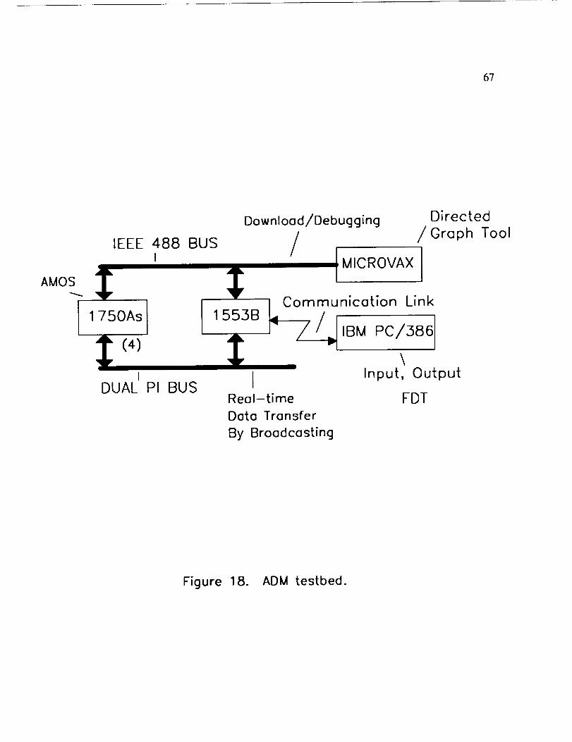
67

AMOS

IEEE 488 BUSI

Download/Debugging

/MICROVAX

Directed

/ Graph Tool

1750As

(4)

IDUAL PI BUS

_ Communication Link1553B

/ / _ _BMPc/3a6\

I Input, Output

Reel-time FDTData Transfer

By Broadcasting

Figure 18. ADM testbed.

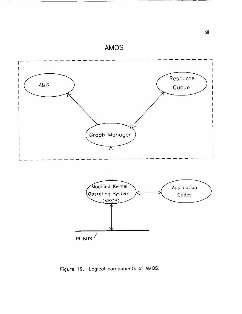
68

AMOS

AMG

Resource

Queue

Graph Manager

PI BUS /

,dified Kernel

g System

I

Figure 19. Logical components of AMOS.

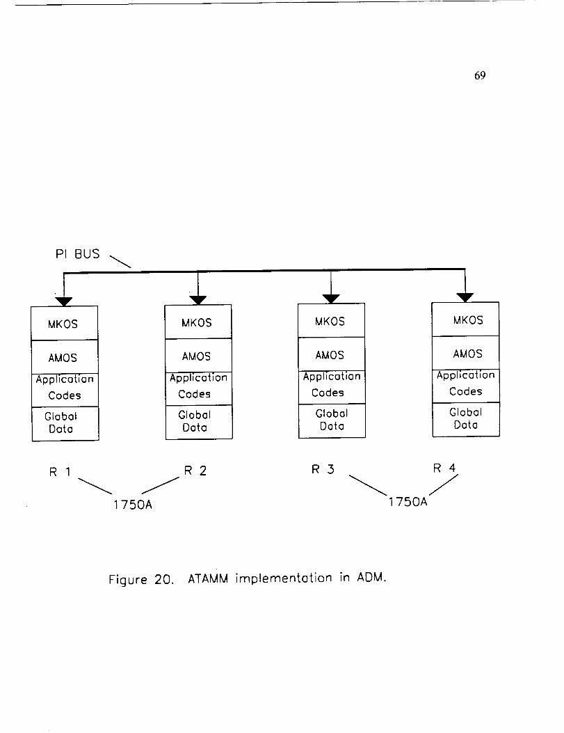
69

PI BUS

MKOS

AMOS

Application

Codes

GlobalData

MKOS

AMOS

Application

Codes

GlobalData

MKOS

AMOS

Application

Codes

GlobalData

$MKOS

AMOS

Application

Codes

GlobalData

R 1 R2 R3

1750A

R 4

1750A

Figure 20. ATAMM implementation in ADM.

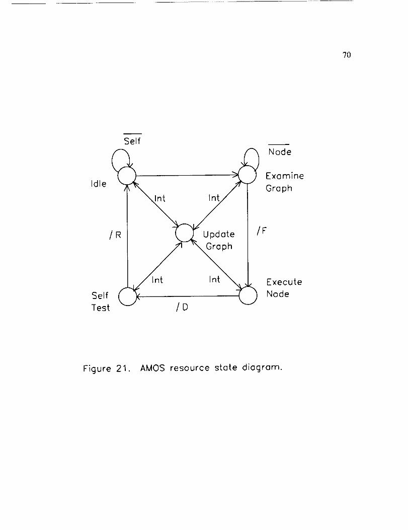
7O

Self

Node

Idle

Int Int

Examine

Graph

/R

Self (Test / D

Update

Graph

Int

/F

Execute

Node

Figure 21. AMOS resource state diagram.

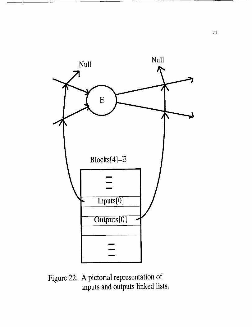
71

NullNull

Outputs

m

m

B

Figure 22. A pictorial representation ofinputs and outputs linked lists.

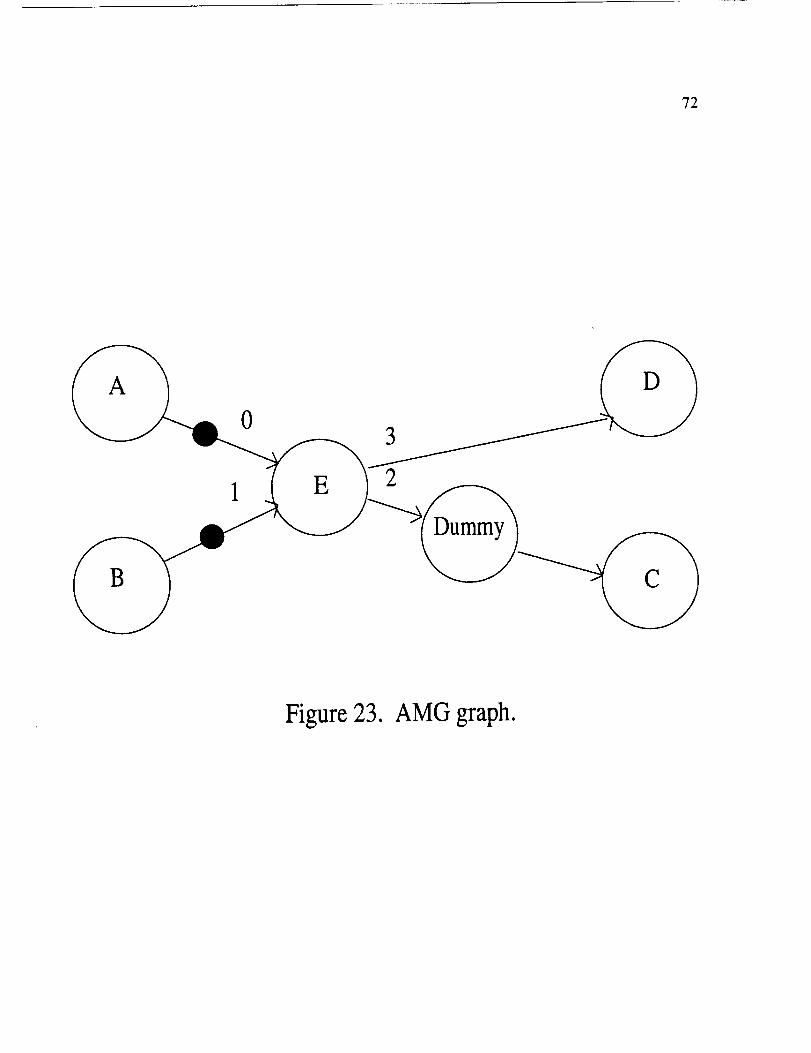
72

A

B

0

1 E

3

2

Dummy

D

C

Figure 23. AMG graph.

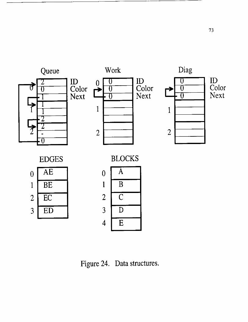
73

Queue

ColorNext

1.22

02

Work

.0

Diag

ID _ IDColor ColorNext Next

1

2

0

1

2

3

EDGES

AE

BE

EC

ED

0

1

2

3

4

BLOCKS

A

B

C

D

E

Figure 24. Data structures.

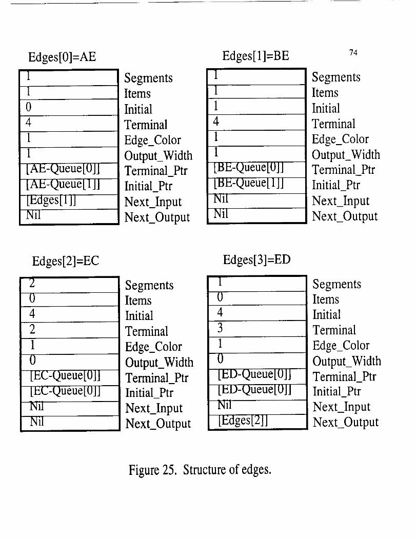
Edges[0]=AE

1

1

0

411

[AE-Queue[OJ][AE-queue[ ]11

[Edges[i]]Nil

SegmentsItems

Initial

Terminal

Edge_Color

Output_WidthTerminal_PtrInitial Ptr

Next_inputNext_Output

Edges[1]=BE

1

14

11

[BE-Queue[0]]

[Bg-queue[lJ]NilNil

74

SegmentsItems

Initial

Terminal

Edge_Color

Output_WidthTerminal_PtrInitial Ptr

Next__Input

Next__Output

Edges[2]=EC

2

04

2

10

[EC-Queue[0]][t';C-Queue[0l]NilNil

SegmentsItemsInitial

Terminal

Edge_Color

Output_WidthTerminal PtrInitial_Ptr

Next_Input

Next_Output

1

04

3

1

0

Edges[3]=ED

i [gD-Queue[0]l

' _[_gO_Queue[ollNil

[gdges[2]]

SegmentsItems

Initial

Terminal

Edge_Color

Output_WidthTerminal PtrInitial_Ptr

Next_input

Next_Output

Figure 25. Structure of edges.

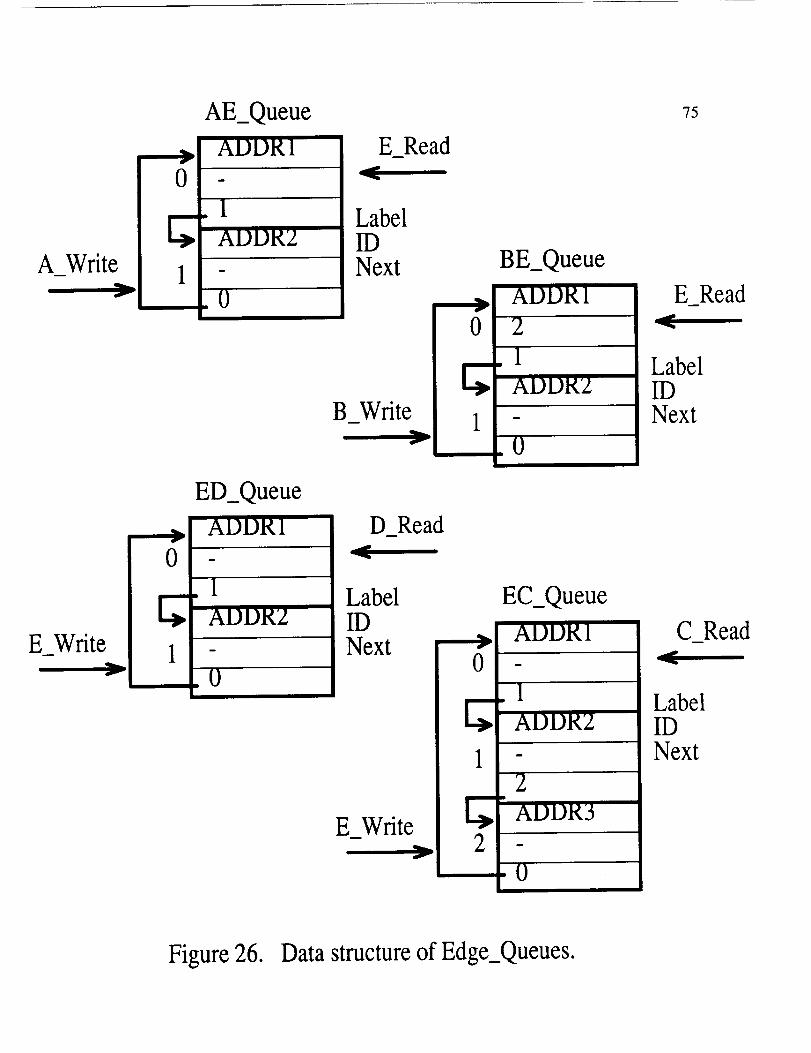
A Write

f

0

J

1

AE_Queue

ADDR1

m

1ADDR2

0

E Readm

LabelIDNext

B Write

0

J

BE_Queue

ADDR1

21ADDR2

0

75

E Read

LabelIDNext

E Write

0

ED_Queue

ADDR1

1ADDR2

D

0

D Read

LabelIDNext

E_Write

EC_Queue

0

J

ADDRI

1ADDR2

2

C Read

LabelIDNext

Figure 26. Data structure of Edge. Queues.

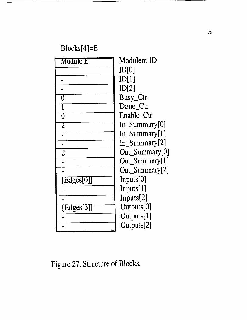
76

Blocks [4]=E

MoOule P.,

i

0102

2

I iEdges[O]]

I !Edges[ 3]]

Modulem ID

ID[0]ID[1]ID[2]

Busy_CtrDone CtrEnab__Ctr

In_Summary[0]In_Summary[ 1]In_Summary[2]OuLSummary[0]Out_Summary[l]Out_Summary[2]

Inputs[0]Inputs[l]Inputs[2]Outputs[0]Outputs[l]Outputs[2]

Figure 27. Structure of Blocks.

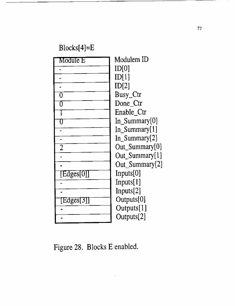
77

Blocks[4]=E

lz Modulem ID- ID[O]

ID[1]ID[2]

Busy_CtrDone CtrEnable Ctr

In_Sul_mary[0]

In_Summary[ 1]In_Summary[2]OuLSummary[0]Out_Summary[l]OutSummary[2]Inputs[0]Inputs[l]Inputs[2]Outputs[0]Outputs[I]Outputs[2]

Figure 28. Blocks E enabled.

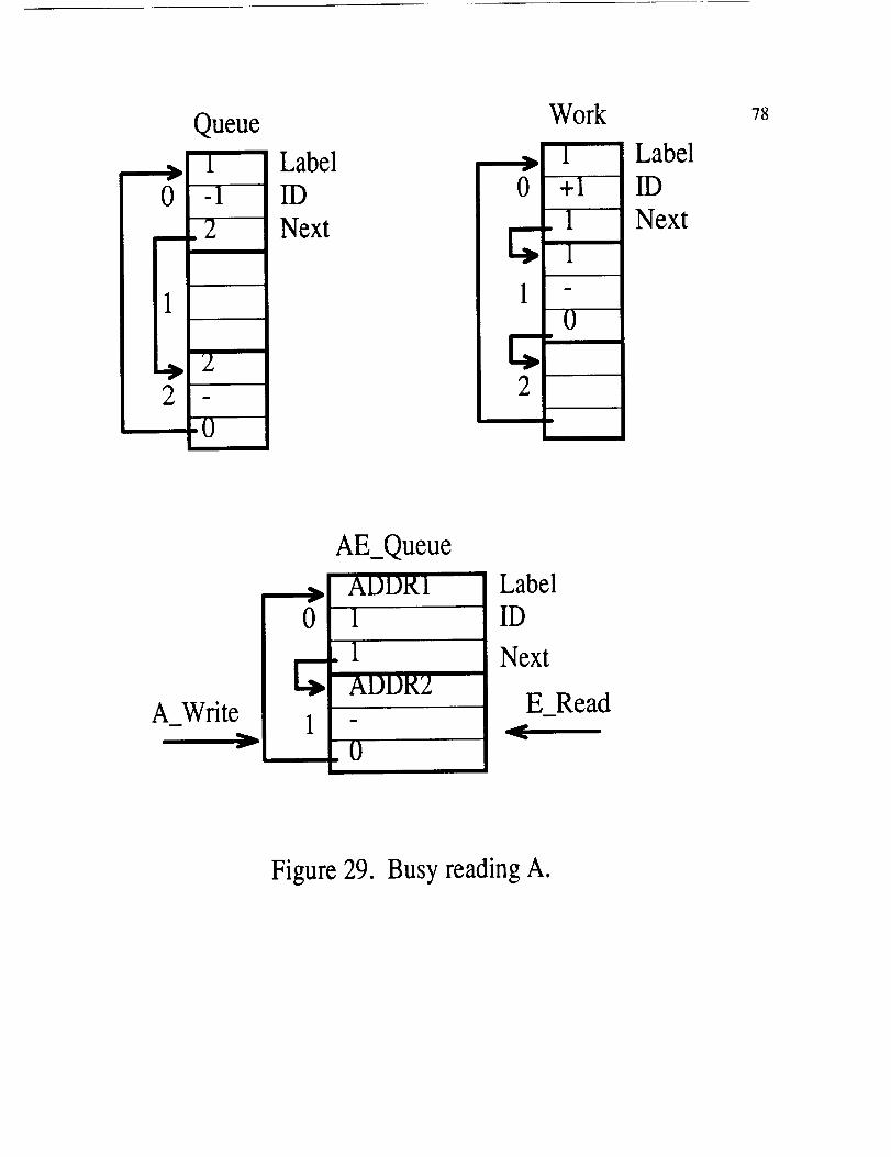
0

1

2

Queue

1

-1

.2

2

m

0

Label

IDNext

qh._l

0

1

J

2

Work

1

+1

1

1m

0

Label

IDNext

78

A Write

6J

i.._I

AE_Queue

ADDR1

1

1

ADDR2

0

Label

ID

Next

E Readw

Figure 29. Busy reading A.

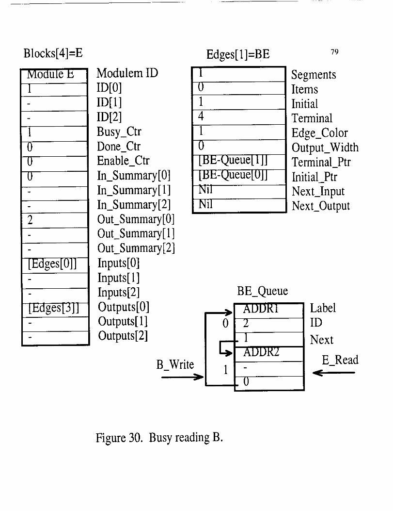
Blocks[4]=EEdges[1]=BE

Modulem IDID[0]ID[1]ID[2]

Busy_CtrDone_CtrEnable CtrIn_Summary[0]In_Summary[1]In Summary[2]Out_Summary[0]Out_Summary[I]Out_Summary[2]Inputs[0]Inputs[l]Inputs[2]Outputs[0]Outputs[I]Outputs[2]

1

41

_llI

B_Write

0

!

BE_Queue

ADDRI2

.1ADDR2

79

SegmentsItems

InitialTerminal

Edge_ColorOutput_WidthTerminal_Ptr

I Initial_Ptr

i Next_InputNext_Output

Label

ID

Next

ERead

Figure 30. Busy reading B.

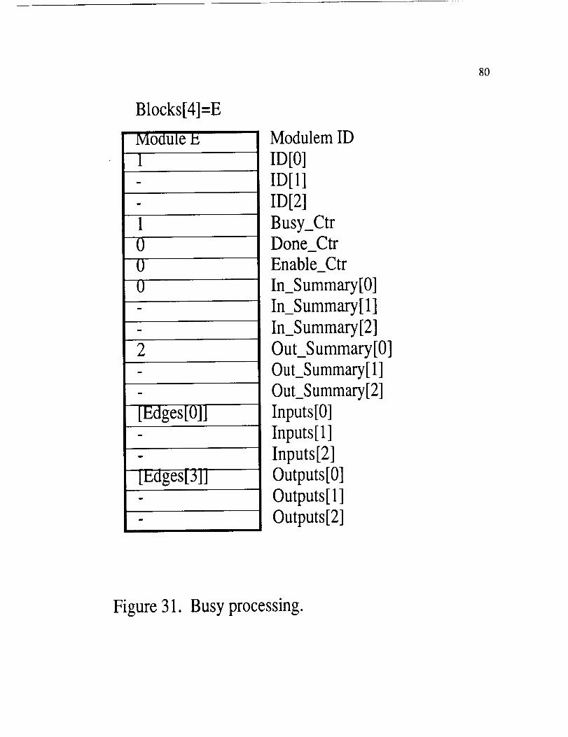
80

Blocks[4]=EModulem II3

ID[0]ID[1]ID[2]Busy_CtrDone_CtrEnable_CtrIn Summary[0]In Summary[l]In_Summary[2]Out_Summary[0]Out_Summary[l]Out_Summary[2]

Inputs[0]Inputs[I]Inputs[2]Outputs[0]Outputs[l]Outputs[2]

Figure 31. Busy processing.

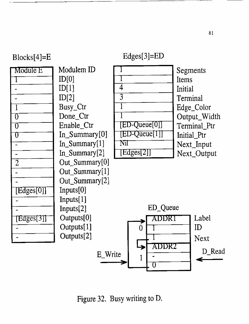
81

Blocks[4]=E

Module E

1

m

10

00

B

2

m

[Edges[0]]

[Edges[3]]

Modulem ID

ID[O]ID[I]

ID[2]

Busy_CtrDone Ctr

Enable Ctr

In_Summary[0]

In_Summary[I]

In_Summary[2]Out_Summary[0]

OutSummary[1]

Out_Summary[2]Inputs[0]

Inputs[l]Inputs[2]

Outputs[0]Outputs[I]Outputs[2]

1

4

3

1

Edges[ _I=ED

E Write

1

[ED-Oue Je[011

lED-Queue[IllNil

[Edges[; II

f

0

1

ED_Queue

ADDR1

1

1

ADDR2

0

SegmentsItemsInitial

Terminal

Edge_ColorOutput_WidthTerminal PtrInitial Ptr

Next_InputNext_Output

Label

ID

Next

D Read

Figure 32. Busy writing to D.

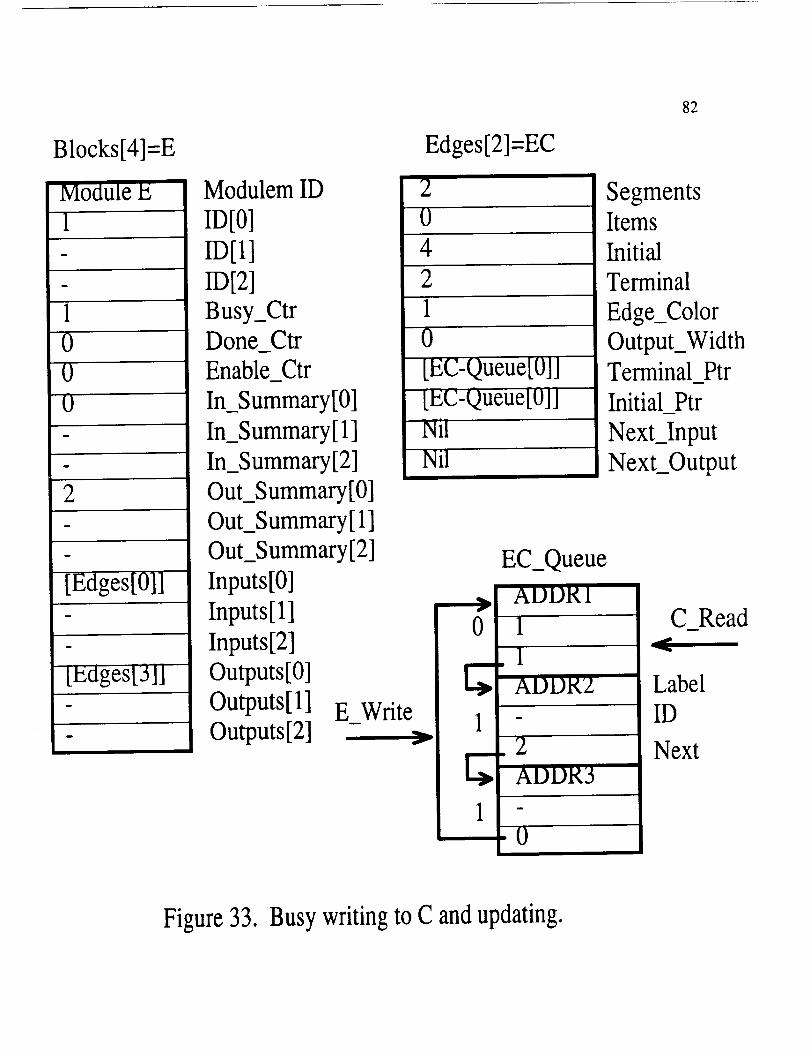
Blocks[4]=E

' Module E

1

10

0O

2

m

I [Edges[Oil

I tLdges[31i

Edges[2]=EC

Modulem ID

ID[O]

ID[I]

D[21Busy_CtrDone Ctr

Enable_Ctr

In_Summary[0]

In_Summary[ 1]

In_Summary[2]Out_Summary[0]

Out_Summary[ 1]Out_Summary[2]

204

210

J _C-Oueuel01]

[EC-Queue[0]]NilNil

Inputs[0]Inputs[l]Inputs[2] 0

Outputs[0]Outputs[l]Outputs[2] EsWrite_ 1

1

EC_Queue

ADDRI

1

ADDR2

2

ADDR3

0

82

SegmentsItems

InitialTerminal

Edge_Color

Output_WidthTerminal Ptr

Initial Ptr

Next_Input

Next_Output

C Read

LabelID

Next

Figure 33. Busy writing to C and upaating.

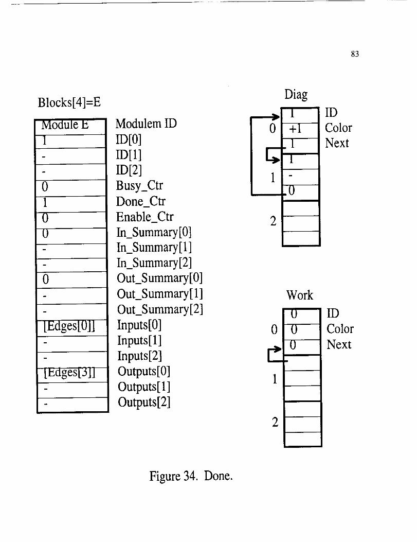
83

Blocks[4]=E

Module E Modulem ID

1 ID[O]

- ID[1]- D[2]

0 Busy_Ctr1 Done_Ctr0 Enable_Ctr

0 In_Summary[0]

- In_Summary[I]In_Summary[2]

0 Out_Summary[0]

Out_Summary[1]Out_Summary[2]

lEdges[0]] Inputs[0]

Inputs[l]

Inputs[2]

[Edges[3]] Outputs[0]Outputs[l]Outputs[2]

Diag

',---, l

0 +1

L._ 1

1 -0

2

Work

U

0 0

0n

1

2

ID

ColorNext

IDColor

Next

Figure 34. Done.

rI

/

L

Idle, Examine Graph

IdleJ

On-Hold-Read

j'%

R

Self Test

Execute Node

Update

On-Hold-Update

TTest

I

III

I

ff--

I

Write J

%,

Update

Read

Process

84

On-Hold-Write

Update

Figure 35. Functionalunit operations.

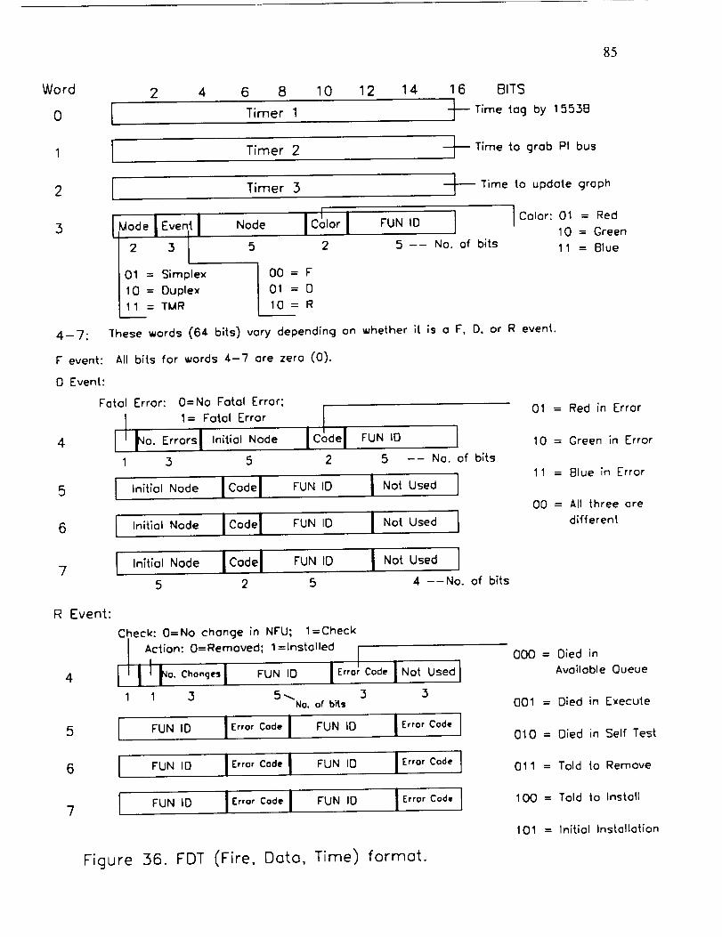
85

Word

0

2 4 6 8 10 12 14

I Timer 1

16 BITS

-_--Time tog by 15538

l Timer 2 J_ Time to grab PI bus

3

4-7:

Timer 3

_odeIEventI

O1 = Simplex

IO = Duplex

11 = TMR

00=F

01=0

10=R

FUN ID [

5 -- No. of bits

---_ Time update graphto

Color: = Red0 1

10 = Green

1 1 = Blue

These words (64 bits) vary depending on whether it is o F, D, or R event.

r event: All bits for words 4-7 ore zero (0).

O Event:

4

Fatal Error: 0=No Fatal Error;

o. Errors Initial Node C de

1 3 5 2

5 I InitFal Node JCodeI FUNID

6 Initial Node icodel FUN ID

FUN IO ]

5 -- No. of bits

I N°t Used I

I N°t Used I

01 = Red in Error

10 = Green in Error

11 = Blue in Error

00 = All three ore

different

7 InitialNode I codel FUN ID I NotUsed J5 2 5 4 --No. of bits

R Event:

4

5

6

Check: O--No change in NFU; l=Check

I Action: O=Removed; 1=Installed

1 1 3 5-_ 3 3No, of b_s

l FUNID I Error Code I FUNIO I Error Code )

[ FUNID I Error Code I FUN 113 I E-o, Code I

0DO = Died in

Available Queue

001 = Died in Execute

010 = Died in Self Test

011 = Told to Remove

7 I FUNID IE.o,co.i FUNID IE.o,co ,I 100 = Told to Install

101 = Initial Installation

Figure 56. FDT (Fire, Data, Time) format.

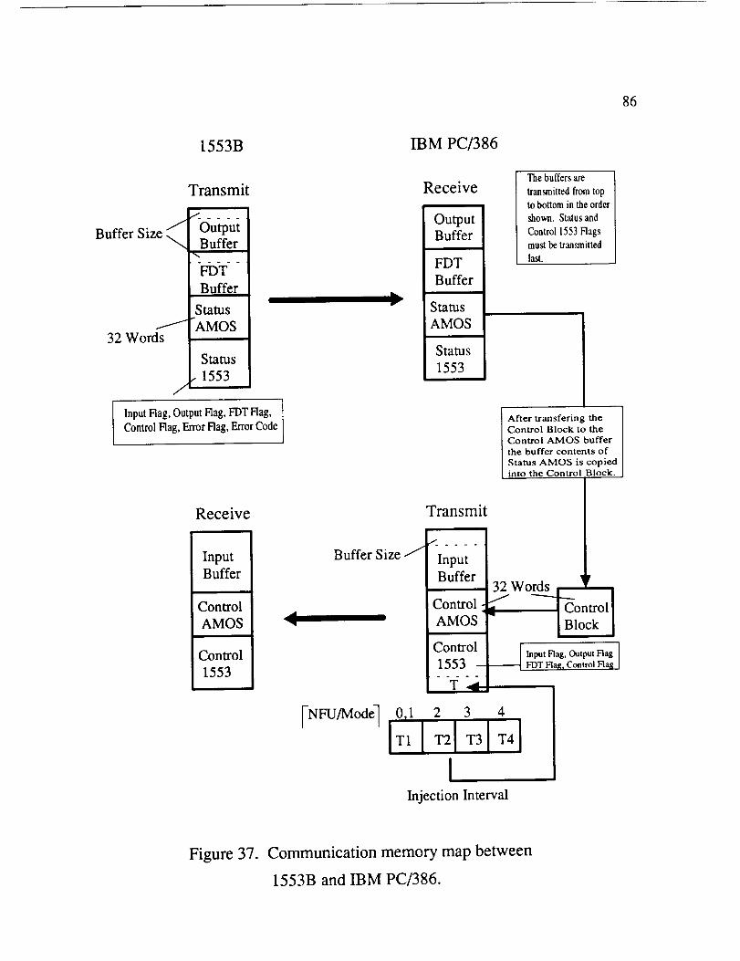
86

1553B

Buffer Size

J32 Words

/

Transmit

OutputBuffer

FDT

Buffer

Status

"AMOS

Status

,. 1553

Input Flag, Output Flag, FDT Flag,

Control Flag, Error Flag, Error Code

IBM PC/386

Receive

OutputBuffer

FDT

Buffer

" Status

AMOS

Status

1553

The buffers are

transmitted from topto bottom in the order

shown. Status and

Control 1553 Flags

must be transmitted

last.

After transfering theControl Block to theControl AMOS bufferthe buffer contents of

Status AMOS is copiedinto the Control Block.

Receive

Input

Buffer

Control

AMOS

Control

1553

II

Transmit

Buffer Size J

NFU/Mode-]

InputBuffer

Control

AMOS

Control

1553

T_

32 Words ' y

I Input Flag, Output Flag IFDT Flagf Control Flag

0T1 2 3 4

IInjection Interval

Figure 37. Communication memory map between

1553B and IBM PC/386.

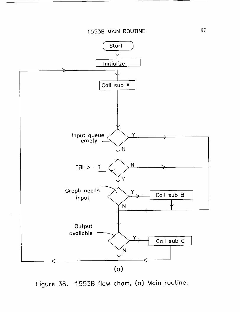
1553B MAIN ROUTINE 87

>

Start .)

fI Initialize ]

f

Input queue Y >empty

N

TBI >= T N >

Graph needs

input

Y

Y

N

Call sub B

< f

<

Output

available

(o)

Call sub C I

<

Figure 38. 1553B flow chart, (a) Main routine.

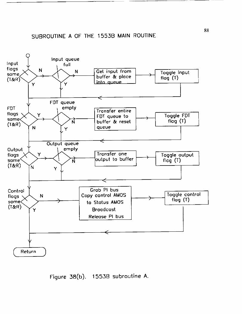
SUBROUTINE A OF THE 1553B MAIN ROUTINE88

Input

flags _ Nsame/\ \ .

(T&R)_ "

FDT _flogs ysame<,. >(T&R) _ /

N

Input queue

full

>

Y

FOT queue

empty

5'

Output queue

I Get input from Ibuffer & place

intn queue

dr_

I Toggle inputflog (T)

Transfer entire

FDT queue tobuffer & reset

queue

Toggle FDT

flog (T)

IOutput .__

\Y .same_(T&R) \N//

Y

I

Control

flogs _ _ysome<,. "(T&R) \

N

>

Transfer one Ioutput to buffer

<

empty

Grab PI bus

Copy control AMOS

to Status AMOS

Broadcast

Release PI bus

Toggle output

flog (T)

__

IToggle controlflog(T)

<

C Return )

Figure 38(b). 1553B subroutine A.

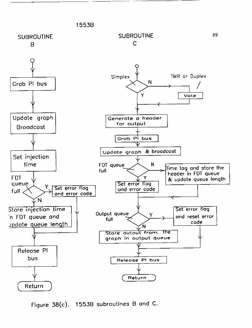
SUBROUTINE

B

1553B

SUBROUTINE

C

89

Grab PI bus

fUpdate graph

Broadcast

i Set injection e_._time FDT queu N

full _-

_YFDT _/queue I , Set error flog

. ,, -_'... Y. ISet error flog ] land error code ]lUll _,_ _ and error code

btore in _ec_" j ion time:n FDT queue and Output que

full ___ 11>

Jpdote queue lenqth . "_..N

t Store output from

Releose PI

bus

Simpl N

<

Generate a header Ifor output

+I_ro__, _u. I

_vJUpdate graph &: broadcast J

)

the

graph in output queue

I-_ ,_°_ p, _°_ I+

rMR or Duplex

I

lime tog and store theheader in FDT queue

& update queue length

i'

%

Set error flag

and reset errorcode

I -t

Figure 38(c). 1553B subroutines B and C.

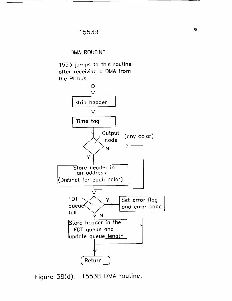
1553B90

DMA ROUTINE

1553 jumps to this routine

ofter receiving o DMA from

the PI bus

I Strip heoder

II_i_°_°_ I

_ode

I( Store heoder in

on oddress

Distinct for eoch color)

Y\f

FOT- queue\ /full y N

tore heoder in the

FDT queue ondpdote queue length

(ony color)

Set error flog

and error code

Figure 38(d). 1553B DMA routine.

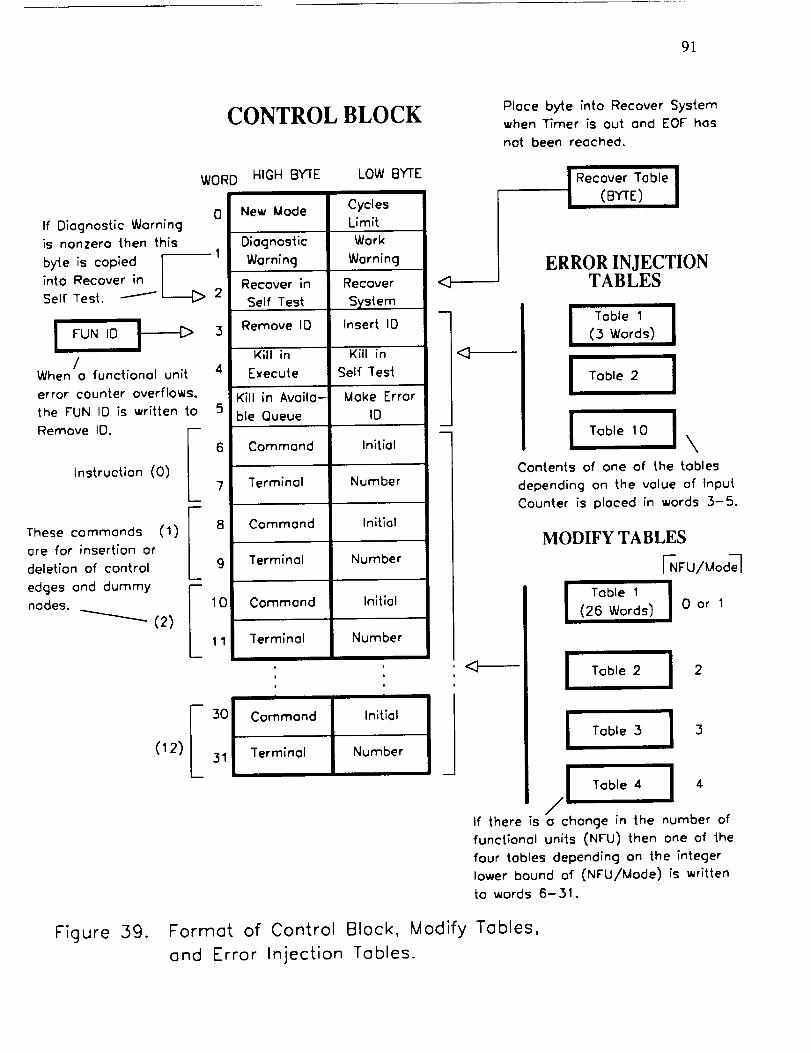
91

CONTROL BLOCK Place byte into Recover System

when Timer is out, and EOF has

not been reached.

WORD

0If Diagnostic Warning

is nonzero then this

byte is copied [-1into Recover in

Self Test,. _ 2

I FUN ID _ 3

/When a functional unit 4

error counter overflows,

the FUN ID is written t,o 5

Remove IO. r 6

Instruction (0) I

L 7

These commands (I) F 8

ore for insertion or Ldeletion of control 9

edges and dummy r-1(]

nodes. _ (2)

11

HIGH BYTE LOW BYTE

New Mode CyclesLimit

Dioqnostic Work

Warning Warning

Recover in

Self Test

Remove IO

Recover

System

Insert ID

Kill in Kill in

Execute Self Test

Kill in Availa- Make Error

ble Queue ID

Command Initial

Terminal Number

Command Initial

Terminal Number

Command Initial

Terminal Number

i

i *

i i

I I

Command Initial

Terminal Number

w

I Recover Table i(BYTE)

ERROR INJECTIONTABLES

lll I

Table 1

(.3Words)

I Toble 2

l Table 10 J X

Contents of one of the tobies

depending on the value of Input

Counter is placed in words .3-5.

MODIFY TABLES

_Fu/Uod_

I I(26 Words] O or 1

I Table 2 I 2

I Table3 I 3

jl Table4 J 4If there is o change in the number of

functional unit,s (NFU) then one of t,he

four tobies depending on the integer

lower bound of (NFU/Mode) is written

to words 6-31.

Figure 39. Format of Control Block, Modify Tobies,

and Error Injection Tobies.

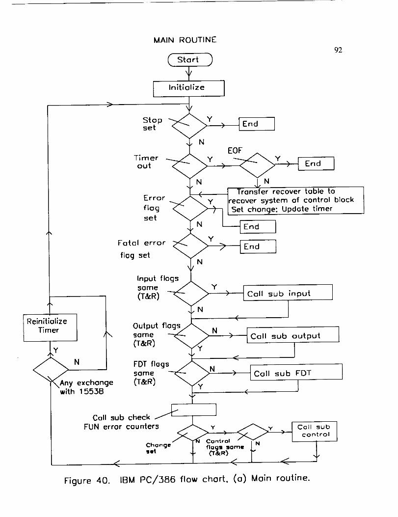
MAIN ROUTINE

Start )

Initialize

92

>

Stop Yset End

Timerout

N

YEOF

End

Error

flog

set

Fatal error

flog set

N

N

N

Y

__N

Transfer recover table to

recover system of control blockSet change: Update timer

End

End

Reinitiolize

TimerN

y exchange

Input flogs

some Y

(T&R)OutmPeut flogs N

FDT flags

some _ % N

with 1553B (T&R)

<

>

I CoII sub input

ICoil sub output

I Call sub FDT

I

Col, sub check _ I

FUN error counters _y ) _/_.._y

<

I

. I Coil sub" I control

Figure 40. IBM PC/386 flow chart, (a) Main routine.

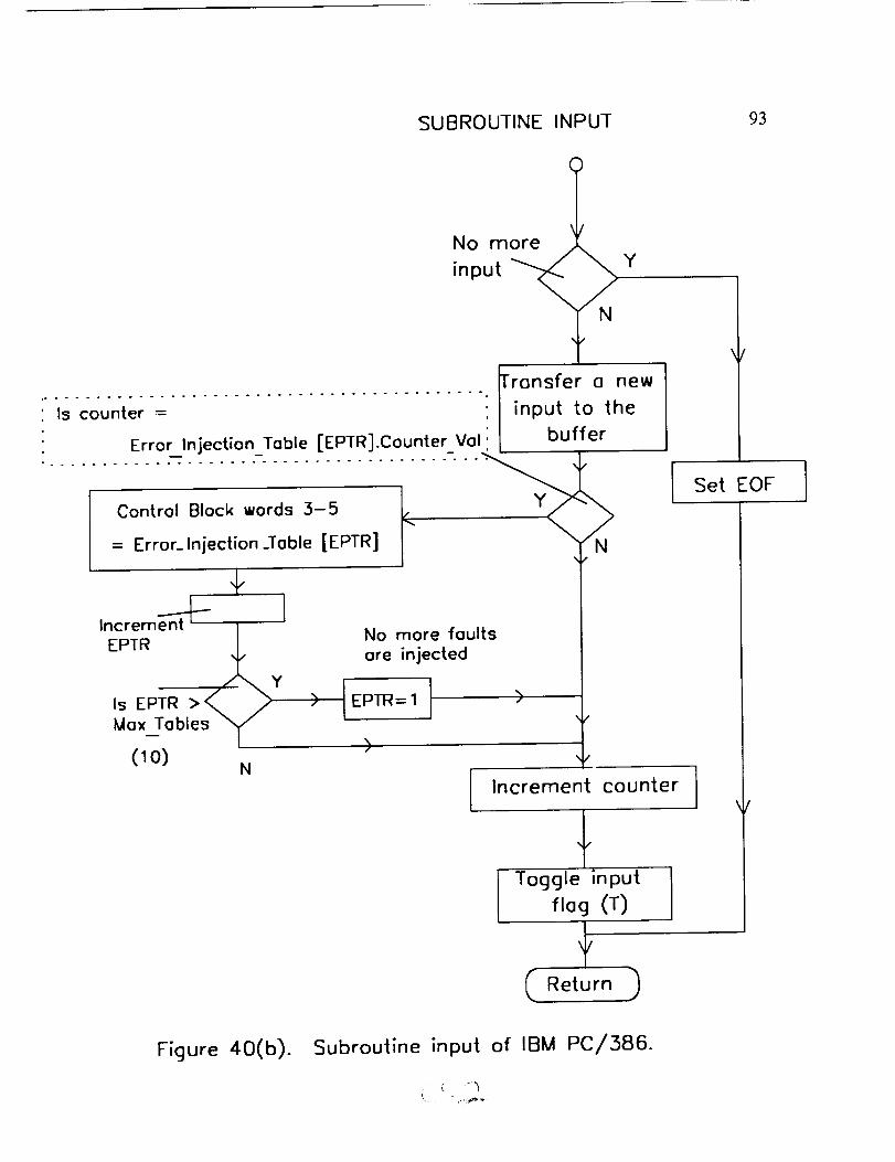
SUBROUTINE INPUT 93

Nom

input _ Y

ronsfer 0 new

'" ls'co'un'ter'- .............................. i/input to the

Error Injection Table [EPTR] Counter Vol I | buffer

Control Block words 3-5 _.

= Error_Injection_Table [EPTR] / \ ;N

Increm ent--'nt-t-_ [

EPTR _ No more faultsare injected

YIsEPTR > % .,,,,2 ,, I IMax Tables " I EPTR=I >

) _"T _/

N I

Set EOF

Increment counter )

I Toggle inputflog (T)

C, Return

Figure 40(b). Subroutine input of IBM PC/386.

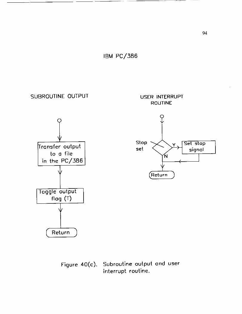
94

IBM PC/386

SUBROUTINE OUTPUT USER INTERRUPT

ROUTINE

Transfer output

to a file

in the PC/386

tIToggle outputflog (T)

Stop

set

rn (

Set stop

signal

I

Figure 40(c). Subroutine output and user

interrupt routine.

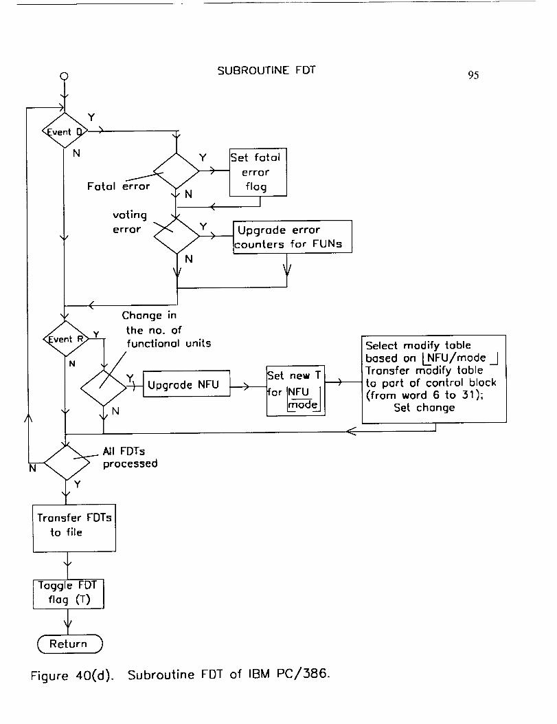
SUBROUTINE FDT 95

N

Y

_Set fatal

_ error

Fatal error YN [ flog

voting _ I-/_.- v

l<

error _, "_Y> IUpgrode error

" Icoun,ers for FUNs

t IChange in

y the no. of

functional units

N

Transfer FDTs

to file

,Fflag CT)

N

Upgrade NFU [, >

:t new TrINFU J -Ga j

All FDTs

processed

<

Select modify table

based on L.NFU/mode_l

Transfer modify tableto port of control block(from word 6 to 31);

Set change

Figure 40(d). Subroutine FDT of IBM PC/386.

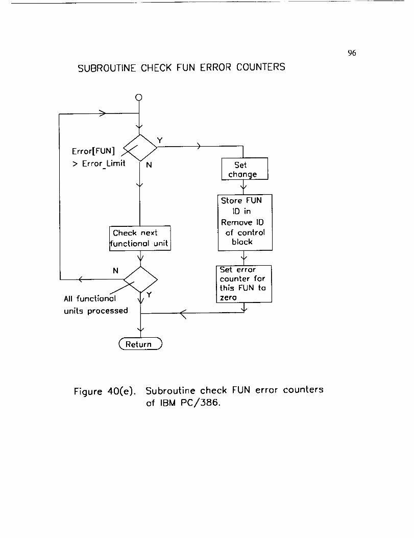
SUBROUTINE CHECK FUN ERROR COUNTERS

96

>

Error[FUN] ,_

> Error Limit N

Check next Ifunctional unit

All function

units processed

(Return)

<

ISet

chonge

Store FUN

ID in

Remove ID

of control

block

Set errorcounter for

this FUN to

zero

$

Figure 40(e). Subroutine check FUN error counters

of IBM PC/386.

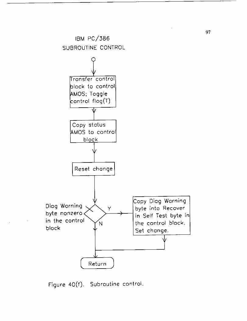
IBM PC/386

SUBROUTINE CONTROL

fronsfer control

talock to control

AMOS; Toggle:ontrol flag(T)

TCopy status

AMOS to contro

block

fI Reset change

9?

Diag Warning xj N_ybyte nonzero <"in the control

block

)

Copy Diag Warning

byte into Recover

in Self Test byte in

the control block.

Set change.

t

Figure 40(f). Subroutine control.

CHAPTER FIVE

ATAMM SUPPORT TOOLS

In order to facilitate the prediction of performance and resource requirements in

an ATAMM defined testbed like ADM, a number of software support tools have been

developed [9, 10, 11]. The ATAMM support tools include software tools named as

Design Tool, Simulator, and Analyzer. The Design Tool is used to select an operating

point for each possible value of available resource. The Simulator is used to simulate

algorithm execution by AMOS on the ADM. Finally, the Analyzer is used to

determine algorithm performance from FDT file outputs produced either by the

Simulator or the ADM hardware. The order in which tools are used is described in

Figure 41.

The software tools are developed in Windows 2.1 running under MS-DOS on

IBM PC/386 or compatible. The programming language used for coding is C. Each

tool consists of several component pieces called windows. Each window is

constructed to solve a particular portion of the total problem. The displays of the

ATAMM support tools are divided in these windows. Several dialogue boxes and

message boxes are provided for the convenience of the user when running the tools.

All options are menu driven and minimum keyboard interaction is required. Each

display of the support tools can be selected from a main window. Any number of

98

99

displayscanappearon the screenat the sametime anda displaycanbe removedfrom

the screenat anytime.

The DesignTool is requiredfor makingoff-line schedulingdecisionsandfor

performanceprediction of algorithms. The DesignTool obtainstherequiredinput

information from the AMG drawnusinga grapheditor. This window allows the user

to create,modify, andstoretheAMG. The most importantoutputof the DesignTool

is the performanceplanewindow which showsall operatingpoints for a particular

algorithmmarkedgraphandenablesthe userto choosea particular setof operating

points. Basedon theuserselection,the DesignTool generatesa modify tablewhich

specifiescontrol edges,buffer sizes,performance,andresourcerequirementsfor each

operatingpoint selectedfrom the performanceplane. A Simulatorhasbeencodedto

simulateand testAMOS. The input parametersfor the Simulatorare the algorithm

markedgraphincluding all NMG transitiontimes,the numberof resources,and

systemoverheadtimessuchas busaccesstime, busbroadcasttime, etc.. The input

injection interval actuallyusedin the Simulatorandhardwaresystemsis determined

by addinga small overheadtime to the DesignTool interval to accountfor bus

contentiontime, functionalunit test time, and increasesin algorithmnodetimesdue to

interruptsfrom otherfunctional units. The Simulatorreportsall eventsassociatedwith

the executionof algorithmnodesfor eachdatapacketon a graphdiagnosticfile, called

the FDT (Fire, Data,Time) file. The Analyzerhasbeendevelopedto determine

algorithmperformanceusingthe FDT file producedby the Simulatoror actual

hardware. It providesthe meansto examinetheoverall systembehaviorto obtain

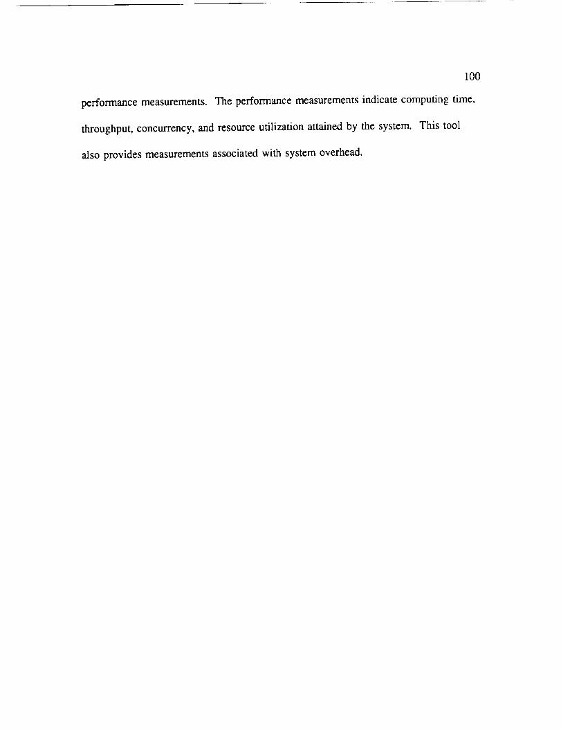
100

performance measurements. The performance measurements indicate computing time,

throughput, concurrency, and resource utilization attained by the system. This tool

also provides measurements associated with system overhead.

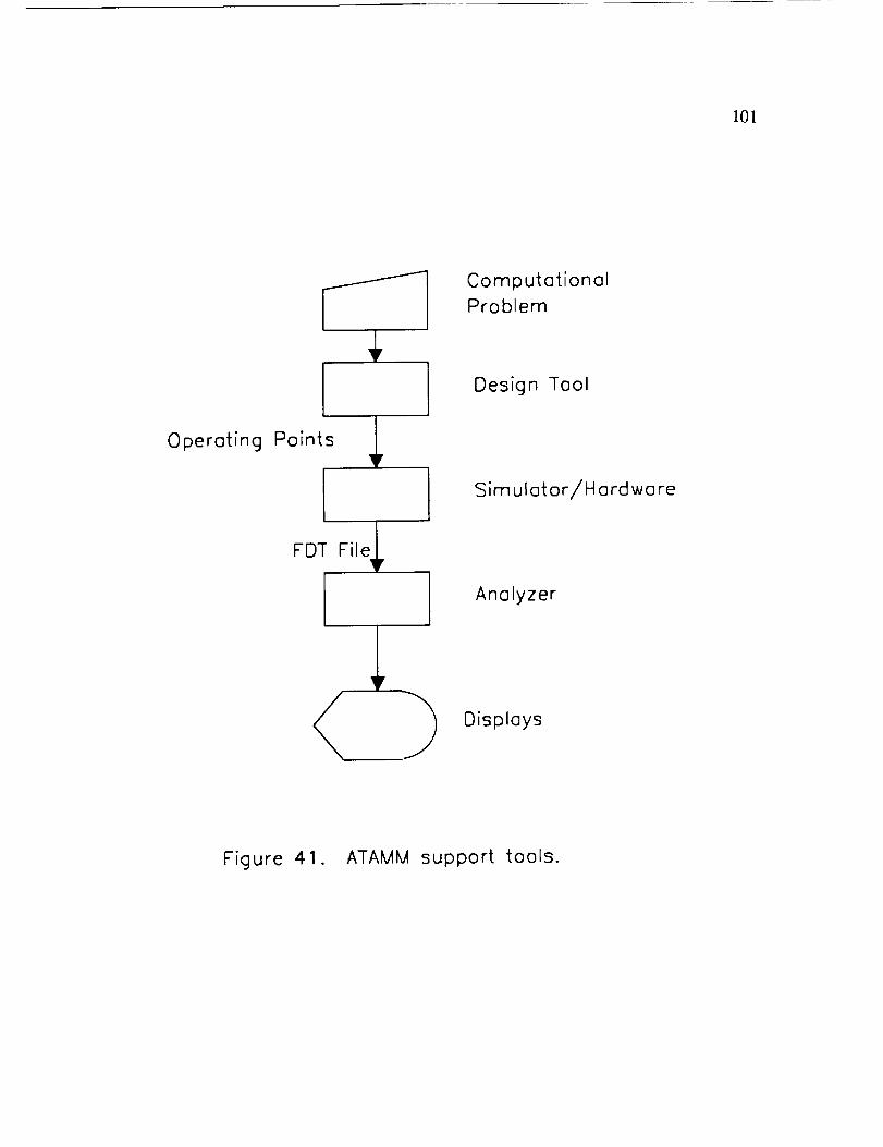
101

Operating Points

FDT

IFile_

Computational

Problem

Design Tool

Simulator/Hardware

Analyzer

Displays

Figure 41. ATAMM support tools.

CHAPTER SIX

RESEARCH STATUS

There are several topics which are the subject of continuing and future

research. Significant progress has been made towards the completion of the ADM

system and it is currently partially operational (three out of four 1750As are

functioning). The ATAMM model is being validated by experiments on the ADM

testbed. A three node algorithm marked graph, shown in Figure 42, has been

successfully executed on the ADM hardware by the NASA Langley Research Center.

A number of algorithms are being analyzed by the ATAMM support tools. A space

surveillance algorithm, described in Figure 43, is to be implemented on the ADM

testbed. The results of design, simulations, experiments, and analysis of this algorithm

will be described in a later report.

The ATAMM model is being extended to include multiple concurrent

instantiations of node operations. Simultaneous execution of multiple algorithm

graphs is being investigated and an overhead model to better account for architecture

dependent parameters such as interprocessor communication and contention in

communication is being developed. Although rare in control and signal processing

algorithms, the model should be extended to include data dependent branching for

completeness. Finally, studies are needed to determine the impact of node time

102

103

variations,wherenodelatencyis datadependent.Work is now in progressto

incorporatethesefeaturesin anenhancedATAMM modelwhich is to be realizedin

the GenericVHSIC SpaceborneComputer(GVSC) [3].

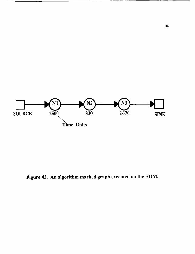
104

SOURCE 2500 830 1670 SINK

"_T_me Units

Figure 42. An algorithm marked graph executed on the ADM.

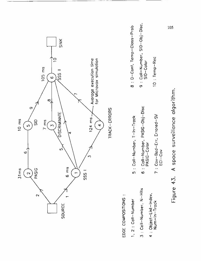
Eo

1.13

E

E

Or)

0

W

I

0

12:I--

d

o i5a. i

J "-"q..D

_ 0o I

E _-_ u

_- E_

o i i EI _r'_ _J_ I---

O (_.)_• , 0.

o

105

C-

6-

0U

D_ m

O_x I

o 0 I (2

I _ "- OI 0

>

Z _ I m

= =m >_=.13 O.,_

0 CJtn ObJ t,.'O

I¢1

.. T _-

¢/I Z "0Z

U"I :3 _ _1--o 7 E _n I _ I c

"_ _ _ "-" Io o ± _uE

CO o4

W _-- _

©

II

L__

REFERENCES

[1] J. W. Stoughton and R. R. Mielke, "Petri-Net Model for Concurrent Processing

of Complex Algorithms,"Proceedings of Government Microcircuit Applications

Conference, San Diego, CA, November 1986.

[2] R. R. Mielke, John W. Stoughton, and Sukhamoy Som, "Modeling and

Performance Bounds for Concurrent Processing," Proceedings of the 8th

International Conference on Distributed Computing Systems, San Jose, CA,June 1988.

[3] R. Mielke, J. Stoughton, S. Som, R. Obando, M. Malekpur, and B. Mandala

"ATAMM Multicomputer Operating System Functional Specification," NASA

Contractor Report, Grant NCC 1-136, August 1990.

[41 J. L. Peterson, Petri Net Theory and the Modeling of Systems, Englewood

Cliffs, NJ, Prentice Hall, 1981.

[5] R. R. Mielke, John W. Stoughton, and Sukhamoy Som, "Modeling and

Optimum Time Performance for Concurrent Processing," NASA Technical

Paper 4167, Grant NAG-I-683, August 1988.

[6] Sukhamoy Som, "Performance Modeling and Enhancement for the ATAMM

Data Flow Architecture," Ph.D. Dissertation, Old Dominion University,

Norfolk, VA, May 1989.

[7] S. Som, J. W. Stoughton, and R. R. Mielke, "Performance Modeling in the

ATAMM Data Flow Architecture," Proceedings of the Ninth IEEE International

Phoenix Conference on Computers and Communications, pp. 163-169,

Scottsdale, Arizona, March 21-23, 1990.

[8] S. Som, R. R. Mielke, and J. W. Stoughton, "Strategies for Predictability in

Real-Time Data-Flow Architectures," Proceedings of the 1 lth IEEE Real-Time

System Symposium, Orlando, Florida, pp. 226-235, December 5-7, 1990.

[9] Robert L. Jones, III, "Diagnostic Software for Concurrent Processing Computer

Systems," Master's Thesis, Old Dominion University, April 1990.

106

[101

[11]

[12]

[13]

107

Brij Mohan V. Mandala, "A software Design Tool for Predictable Performance

in Real-Time Data Flow Architectures," Master's Thesis, Old Dominion

University, December 1990.

M. Malekpour, R. Obando, R. R. Mielke, and J. W. Stoughton, "ATAMM

Simulation Tool for Data Flow Architectures," Proceedings of the 21st Annual

Pittsburgh Conference on Modeling and Simulation, pp. 953-957, May 3-4,1990.

Vason P. Srini, "An Architectural Comparison of Dataflow Systems,"

Computer, pp. 68-88, March 1986.

E. A. Lee and D. G. Messerschmitt, "Static Scheduling of Synchronous Data

Flow Programs for Digital Signal Processing," IEEE Transactions on

Computers, vol. 36, pp. 24-35, January I987.

Documents

G3 - NASA · Brij Mohan V. Mandala, Graduate Research Assistant Year End Report for 1990 Prepared for National Aeronautics and Space Administration Langley Research Center Hampton,