Embed Size (px)
Citation preview
Physics of the Earth and Planetary Interiors 171 (2008) 7–18
Contents lists available at ScienceDirect
Physics of the Earth and Planetary Interiors
journa l homepage: www.e lsev ier .com/ locate /pepi
Modelling compressible mantle convection with large viscositycontrasts in a three-dimensional spherical shell using theyin-yang grid
Paul J. Tackley ∗
Institute of Geophysics, ETH Hoenggerberg HPP L13, Department of Earth Sciences,ETH Zurich 8093, Switzerland
a r t i c l e i n f o
Article history:Received 30 October 2007Received in revised form 15 July 2008Accepted 4 August 2008
Keywords:Mantle convectionYin-yang gridMultigridSpherical shell
a b s t r a c t
Here it is documented how an existing code for modelling mantle convection in a cartesian domain,Stag3D, has been converted to model a 3D spherical shell by using the recently introduced yin-yanggrid. StagYY is thus the latest evolution of a code that has been in continuous use and developmentfor about 15 years so incorporates much physics and several features including compressibility, phasetransitions, compositional variations, non-linear rheology, parallelisation, tracers to track composition,partial melting and melt migration, and the ability to also model spherical patches, cartesian boxes,and various 2D geometries by changing one input switch. StagYY uses a multigrid solver to obtain avelocity–pressure solution at each timestep on a staggered grid, a finite-volume scheme for advectionof temperature and tracers to track composition. Convergence of multigrid solvers in the presence ofrealistically large viscosity variations has always been a problem; here a new pressure interpolationscheme is presented that can dramatically improve the robustness of the iterations to large viscos-ity variations, with up to 19 orders of magnitude variation in presented tests. Benchmark tests showthat StagYY produces results that are consistent with those produced by other codes. Performance testsshow reasonable scaling on a parallel Beowulf cluster up to 64 CPUs, with up to 1.2 billion unknowns
solved for in a few minutes. StagYY is designed to be a stand-alone application with no librariestalled
1
hG11hbCymauv
rpoowasoahc
0d
required and if MPI is insdiscussed.
. Introduction
Mantle convection calculations in 3D spherical shell geometryave often used a spectral method (e.g., Bercovici et al., 1989a;latzmaier, 1988; Harder and Christensen, 1996; Machetel et al.,995; Monnereau and Quere, 2001; Tackley et al., 1994; Young,974; Zhang and Christensen, 1993; Zhang and Yuen, 1996). Due,owever, to limitations in the lateral viscosity contrasts that cane handled with a spectral method (Balachandar et al., 1996;hristensen and Harder, 1991; Zhang and Christensen, 1993), recentears have seen a surge of interest in developing grid-based
ethods using finite-element, finite-difference or finite-volumepproximations. While a simple (longitude, latitude) grid has beensed (Ratcliff et al., 1995; Yoshida et al., 1999), it has the disad-antage that the grid lines converge at the poles, causing uneven
∗ Fax: +41 44 633 1065.E-mail address: [email protected].
pf(tnH
(Y
031-9201/$ – see front matter © 2008 Elsevier B.V. All rights reserved.oi:10.1016/j.pepi.2008.08.005
it can be run in parallel. Technical issues and goals for the future are
© 2008 Elsevier B.V. All rights reserved.
esolution, limiting the timestep and possibly causing convergenceroblems for iterative solvers. Various grids have been proposed tovercome this “pole problem” and give a more uniform grid spacingr element size. The first such grid to be used for mantle convectionas the isocahedral grid (Baumgardner, 1985, 1988), in which the
zimuthal discretization uses triangles suitable for a finite-elementolver. A different finite-element discretization using several non-rthogonal rhombahedral patches was implemented by Zhong etl. (2000). The “cubed sphere” grid (Ronchi et al., 1996), on the otherand, is suitable for either finite-difference or finite-element dis-retizations, and consists of dividing the sphere into six patches byrojecting a cube onto a sphere. In its simplest form as implementedor mantle convection by Choblet (2005), Hernlund and Tackley2003) the grid lines are non-orthogonal, requiring many addi-ional terms in the resulting finite-difference equations. A modified,
early orthogonal version has however been found by Harder andansen (2005), Stemmer et al. (2006).The so-called “yin-yang” grid proposed by Kageyama and Sato2004) and first applied to the mantle convection problem byoshida and Kageyama (2004, 2006) has the advantage that it is
8 nd Pla
ngatnspaostoaswtus(
tKoico“maalstiTirdmgTtFot
2
2
iaedeadsowwcu
3dmtp
d
∇m
∇
a
�
Is
Ttεnbti�ae
2
eocaiartcnodw
cetstm
pct
P.J. Tackley / Physics of the Earth a
aturally orthogonal. This grid consists of two (longitude, latitude)rids each stretching ±45◦ in latitude by 270◦ in longitude thatre combined like the two patches of a tennis ball or baseballo make a sphere. The main advantage of this grid over alter-atives is that the grid lines remain orthogonal and therefore aimple discretization such as finite-differences can be used, sim-lifying the implementation and, for example, allowing one to takedvantage of various advection techniques that have been devel-ped in the atmospheric community on orthogonal grids. The gridpacing various by cosine(45◦), i.e.,
√2. A disadvantage is that
he two subgrids do not mesh neatly, unlike the cubed spherer the isocahedral grid, requiring a more complex interpolationt the edge. Additionally, the two subgrids overlap—by 6% if theimple rectangular subgrids are used (Kageyama and Sato, 2004),hich gives the possibility of developing somewhat different solu-
ions in the overlapping areas. This can, however, be minimized bysing a minimum overlap version of the grid, two different ver-ion of which are shown in Figs. 5 and 6 of Kageyama and Sato2004).
In this paper, an implementation of the yin-yang grid for man-le convection is described that advances on that of Yoshida andageyama (2004) in several ways. One way is to use a “minimumverlap” version of the yin-yang grid, namely the version shownn Fig. 5 of Kageyama and Sato (2004), in which any cells at theorners of each subgrid that are completely contained within thether subgrid are removed to produce what they refer to as abaseball-like” border curve. Other improvements are the imple-entation of more complex physics, including the compressible
nelastic equations, phase transitions, compositional variations,nd non-linear rheology, and technical advances including paral-elisation, tracers to track composition, and a pressure interpolationcheme that gives enhanced robustness to large viscosity varia-ions. The code is a development of Stag3D, initially developedn 1992 (Tackley, 1993) and steadily developed since then (e.g.,ackley, 1996, 1998b, 2002; Tackley and Xie, 2003), and thus inher-ts most of the features of that code. The new version of the codeeported here retains the ability to model a 3D or 2D cartesianomain, and in addition to a full “yin-yang” spherical shell can alsoodel a regional spherical block, or the two-dimensional spherical
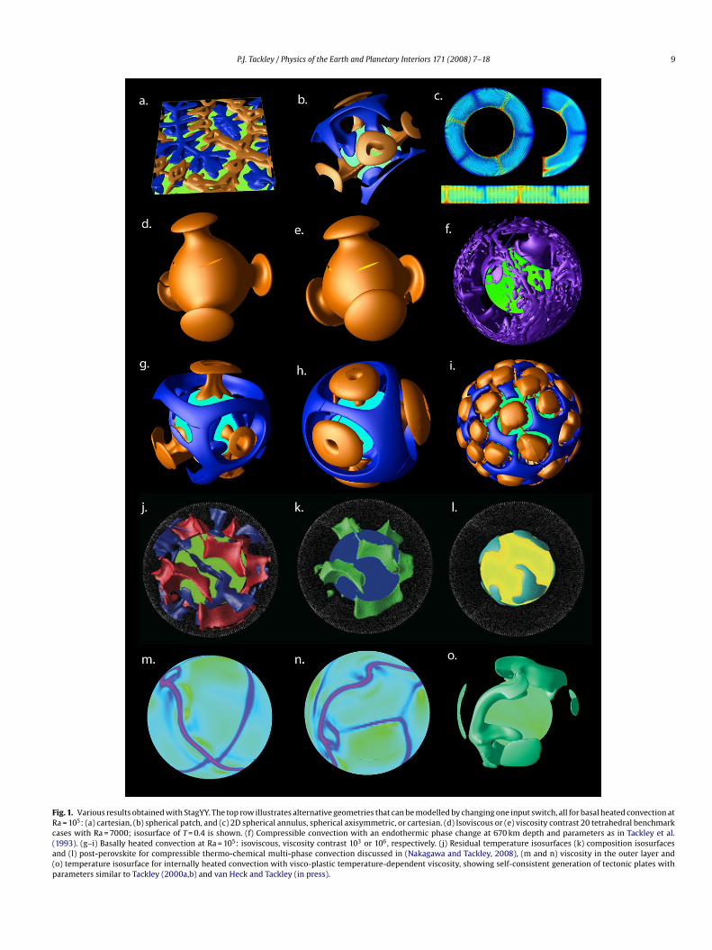
eometries of axisymmetric or spherical annulus (Hernlund andackley, 2008). Results in these alternative geometries are illus-rated in Fig. 1a–c, and have the same parameters as the case inig. 1g. The code is written in Fortran 95 and takes advantagesf features such as dynamic array allocation and derived variableypes.
. Physical model
.1. Approximations and equations
As usual for the solid Earth, the infinite Prandtl number approx-mation is made. Additionally, compressibility is included byssuming the anelastic approximation, in which the continuityquation uses a reference state density rather than the full pressure-ependent density, in order to avoid acoustic waves (e.g., Schubertt al., 2000). In the present version, the “truncated” version of thenelastic approximation is used, which means that the effect ofynamic pressure on temperature is neglected. A quick calculationuggests that this term is unimportant but this should be rigor-
usly tested in the future. Implementing the full anelastic equationsould not add significant complexity and the author has workedith them in the past (Tackley et al., 1993, 1994), but in this appli-ation using the truncated version allows dynamic pressure to besed as a variable rather than total pressure, allowing the use of
aRmtP
netary Interiors 171 (2008) 7–18
2-bit rather than 64-bit precision for the pressure field. That is, asynamic pressure is small compared to total pressure in the deepantle, treating pressure variations accurately enough to enforce
he continuity equation would require 64-bit precision if using totalressure.
These assumptions lead to the following set of equations, non-imensionalised to thermal diffusion scales. Conservation of mass:
· (�v) = 0 (1)
omentum
· � − ∇p = Ra. r̂.�(C, r, T)��thermal
(2)
nd energy
CpDT
Dt= −Dis˛�Tvr + ∇ • (k∇T) + �H + Dis
Ra� : ε̇ (3)
n cases where bulk chemistry is treated the following must also beatisfied:
DC
Dt= 0 (4)
he (non-dimensional) variables are total temperature T, composi-ion C, velocity v and pressure p. � is the deviatoric stress tensor and˙ is the strain rate tensor. The governing parameters are Rayleighumber Ra, internal heating rate H, and surface dissipation num-er Dis. Material properties are density �, thermal expansivity ˛,hermal conductivity k, and specific heat capacity Cp. ��thermals the fractional density variation with temperature (=˛dimensional
Tdimensional) and r is the radius. Viscosity � can vary with temper-ture, depth, strain rate or stress, composition, phase, melt fraction,tc.
.2. Variation of physical properties
The above equations are written and implemented in a gen-ral way such that different dependencies of physical propertiesn temperature, pressure and composition can be used. In thelassical anelastic approximation, density, expansivity, diffusivitynd heat capacity are functions of depth (radius) only, whereasn the Boussinesq approximation they are 1, except in the buoy-ncy term in the momentum equation. To progress to moreealistic models, in StagYY these can alternatively be arbitrary func-ions of temperature, depth, and composition. For example phasehanges can cause density jumps of up to 10% so in the conti-uity equation it can be chosen to use the total density insteadf a reference density—as long as the density being used is notependent on dynamic pressure there is no problem with soundaves.
Phase changes are implicitly included in the density (therebyontributing to buoyancy) and their latent heat is included in thenergy equation by using “effective” values of heat capacity andhermal expansivity (Christensen and Yuen, 1985). Density, expan-ivity, conductivity and viscosity are implemented as functions, sohat different forms can be easily substituted without changing the
ain code.The “standard” method of calculating the temperature and
ressure dependence of these in the context of a multi-phase, two-omponent system has been described in a number of papers overhe years (e.g., Nakagawa and Tackley, 2005; Tackley, 1996; Xie
nd Tackley, 2004), so the reader is referred to these for details.ecently, physical properties calculated from self-consistent mini-ization of free energy to determine stable minerals, coupled to ahermodynamic database, have been implemented using the PER-LEX package (Connolly, 2005), along the lines of Gerya et al. (2006).
P.J. Tackley / Physics of the Earth and Planetary Interiors 171 (2008) 7–18 9
Fig. 1. Various results obtained with StagYY. The top row illustrates alternative geometries that can be modelled by changing one input switch, all for basal heated convection atRa = 105: (a) cartesian, (b) spherical patch, and (c) 2D spherical annulus, spherical axisymmetric, or cartesian. (d) Isoviscous or (e) viscosity contrast 20 tetrahedral benchmarkcases with Ra = 7000; isosurface of T = 0.4 is shown. (f) Compressible convection with an endothermic phase change at 670 km depth and parameters as in Tackley et al.(1993). (g–i) Basally heated convection at Ra = 105: isoviscous, viscosity contrast 103 or 106, respectively. (j) Residual temperature isosurfaces (k) composition isosurfacesand (l) post-perovskite for compressible thermo-chemical multi-phase convection discussed in (Nakagawa and Tackley, 2008), (m and n) viscosity in the outer layer and(o) temperature isosurface for internally heated convection with visco-plastic temperature-dependent viscosity, showing self-consistent generation of tectonic plates withparameters similar to Tackley (2000a,b) and van Heck and Tackley (in press).
1 nd Pla
Dt
2
stiarftbig
3
3
maidtetfi
yattlitstgetlgdinaws
3
fi2tcag2i
e
(
(
(
tfivaraot
nptcivn
∇
absd
ibsmdiKtmabfepgs
0 P.J. Tackley / Physics of the Earth a
etails of this treatment will be elaborated in a future publica-ion.
.3. Geometry and boundaries
While the focus here is on treating a full 3D sphericalhell using the yin-yang grid, a single spherical region or arbi-rary size can also be modelled, and 3D cartesian geometrys maintained as an option. Various related 2D geometries canlso be modelled, including cartesian 2D, spherical axisymmet-ic, and spherical annulus (see Hernlund and Tackley (2008)or details on this). Top and bottom boundary condition areypically isothermal or insulating, and free slip or rigid. Sideoundaries can be periodic, reflecting, or permeable, or are
nterpolated from the other block in the case of the yin-yangrid.
. Numerical implementation
.1. Grid
As is usual (e.g., Brandt (1982), Patankar (1980) and used forantle convection since Ogawa et al. (1991)), velocity components
nd pressure are defined on a staggered grid on which the pressures defined in the center of each cell and velocity components areefined at cell boundaries perpendicular to their direction. This hashe advantages that all derivatives in the momentum and continuityquations involve adjacent points and are second-order accurate inhe case of even grid spacing. Additionally, checkerboard pressureelds are avoided.
As mentioned earlier, StagYY uses the minimum overlap yin-ang grid shown in Fig. 5 of Kageyama and Sato (2004), in whichny cells at the corners of each subgrid that are completely con-ained within the other subgrid are removed to produce whathey refer to as a “baseball-like” border curve. Any loops thatoop over all grid cells must take into account the removed cellsn the corners. Each subgrid acts as the boundary condition tohe other subgrid, with “ghost points” holding velocity and pres-ure values that are linearly interpolated from the interiors ofhe other subgrid. Even for a regular (fully overlapping) yin-yangrid, the locations of these ghost points are different at differ-nt grid levels due to the different grid spacing: for coarser gridshey are further inside the other subgrid. For the minimum over-ap grid it is more complicated to determine the locations of thehost points, and the fact that they are different at each grid leveloes not change. For this minimum overlap grid, the boundary
s also different in detail at different grid levels, but this doesot matter because the solution is still defined everywhere—therere no “gaps”. For computational efficiency, the interpolationeights and the points to be used are pre-calculated once and
tored.
.2. Finite-difference discretization
The equations are expressed in spherical polar coordinates. Theorm of the stress and strain rate tensors and their divergencesn spherical polar coordinates is well known (e.g., Schubert et al.,000) so the full set is not repeated here. It is, however, noted thathey can be written in different ways, which although mathemati-
ally identical lead to a different finite-difference expansion henceslightly different numerical solution. The form of stress diver-ences used here is slightly rearranged from that given on page81 of Schubert et al. (2000) in order to best reflect the phys-
cal meaning of the different terms, as shown in the following
3
a
netary Interiors 171 (2008) 7–18
quations.
∇ • �)r
= −∂p
∂r+ 1
r2
∂
∂r(r2�rr) + 1
r sin
∂
∂(�r sin )
+ 1r sin
∂�r
∂− � + �
r(5)
∇ • �)
= −1r
∂p
∂+ 1
r2
∂
∂r(r2�r) + 1
r sin
∂
∂(� sin )
+ 1r sin
∂�
∂+ 1
r(�r − � cot ) (6)
∇ • �)
= − 1r sin
∂p
∂+ 1
r2
∂
∂r(r2�r) + 1
r sin
∂
∂(� sin )
+ 1r sin
∂�
∂+ 1
r(�r + � cot ) (7)
These stress divergences are expanded in terms of velocitieshen a straightforward finite-difference expansion is applied. Thenite-difference stencil for the equation at each of the staggeredelocity or pressure points is pre-calculated and the stencil weightsre stored. Thus, calculating the residue at that point simplyequires multiplying nearby velocity and pressure values by theppropriate weights and summing. This has the advantage thatnce the stencil weights are calculated, the solution routines arehe same for spherical or cartesian geometry.
A subtlety occurs in the treatment of normal strain rates (henceormal stresses) when density is spatially varying, i.e., for com-ressible cases. The divergence of velocity is then non-zero andhe expressions for normal strain rate contain a −1/3∇ · v. If this isalculated literally from the velocities, then instabilities can occurn an iterative solution procedure, because ∇ · v can be incorrectlyery high or low during early iterations. Thus, it is better to recog-ise that:
· (�v) = 0 = �∇ · v + v · ∇� ⇒ ∇ · v = −v · ∇�
�(8)
nd use v · ∇�/� in the strain rate expressions instead of ∇ · v,ecause velocities are more reliable than gradients of velocity. Thisimply appears as an extra term in the calculation of the finite-ifference stencils.
Viscosity is initially calculated at cell centers where temperatures defined. Calculation of normal stresses requires it at that location,ut viscosity must be interpolated to the centers of cell edges for thehear stress terms. The appropriate type of interpolation (e.g., arith-etic, harmonic, geometric or more complex (Ogawa et al., 1991))
epends on the conceptualization of how the viscosity varies phys-cally (e.g., stepwise, linear, geometric). Recently, Deubelbeiss andaus (2008) compared numerical results with analytic solutions
o determine the accuracy obtained with different interpolationethods, and found that harmonic interpolation gave the most
ccurate results, followed by geometric, with linear (arithmetic)eing much worse. Similar findings were also becoming apparentrom the subduction benchmark (Schmeling et al., 2008). Thus, lin-ar (arithmetic) interpolation should certainly be avoided. In theresent code, geometric interpolation is generally used because itives much better convergence than with linear interpolation, andlightly better than with harmonic interpolation.
.3. Velocity–pressure iterations
The velocity–pressure solution that satisfies the continuitynd momentum equations is obtained by iterations, which are
nd Pla
eevs(
2
IttpioCcsovJ
ct
ı
wtpadttto
ttt
ı
wiapalagaoei
tewte
wfi
c(tw1ipttifiie
sgscie
ı
tfmseat
P.J. Tackley / Physics of the Earth a
ncapsulated into a multigrid cycle as described later. The energyquation is treated explicitly as also discussed later. Here the basicelocity–pressure iteration scheme is described, which has someimilarities and differences to the well-known SIMPLER schemePatankar, 1980).
1. Improve velocity field according to the momentum equationsa. Radial velocity field according to the radial momentum equa-
tions.b. Theta velocity field according to the theta momentum equa-
tions.c. Phi velocity field according to the phi momentum equations.
. Update pressure field to reduce divergence in the continuityequation.a. Calculate pressure correction.b. Calculate velocity correction caused by pressure correction.
n each velocity update (e.g., step 1a), the residue is calculated overhe entire grid, then the correction is calculated and finally addedo the solution, i.e., Jacobi iterations. This has the advantage that therocedure can be parallelised without affecting the result, whereas
f Gauss–Seidel iterations are used then a different result will bebtained when the problem is split between different numbers ofPUs. The disadvantage is that convergence is slower. However, thisan be overcome by using “red–black” iterations, in which two sub-weeps are performed on alternating grid points, like the colouringf squares on a checkerboard. Red–black iterations give better con-ergence than point-by-point iterations of either Gauss–Seidel oracobi varieties (Press et al., 1992).
The correction to each velocity component depends on the sten-il weight and a relaxation parameter ˛m, for example for theheta-velocity:
vi−.5jk = −˛mR mom
i−.5jk /
(∂R mom
i−.5jk
∂vi−.5jk
)(9)
here vi−.5jk
is the theta-velocity at point (i−0.5,j,k) and R momi−.5jk
ishe residue (error) of the theta-momentum equation at the sameoint. The 0.5 in the indices arises because (i,j,k) is the center ofcell, at which pressure is defined; the velocity components areefined at staggered points half a grid spacing from this cell cen-er. For multigrid purposes, ˛ should be less than unity in ordero obtain optimal smoothing (Brandt, 1982; Wesseling, 1992), so isypically set to 0.7. In the absence of multigrid, over-relaxation isptimal, i.e., ˛ > 1.
The pressure correction (step 2a) is calculated using a coefficienthat describes how much changing the pressure at a point changeshe continuity residue (i.e., divergence of density times velocity) athat point:
Pijk = −˛cRcontijk /
(∂Rcont
ijk
∂Pijk
)(10)
here the symbols have similar meanings to those in Eq. (9) and ˛c
s a relaxation parameter generally taken to be 1.0. (∂Rcont/∂P) is notstencil weight because the continuity equation does not includeressure, but it is related to the stencil weights of the momentumnd continuity equations. An important question is how to calcu-ate this, because in principle changing the pressure at one pointffects velocities and pressures in the entire domain, requiring a
lobal solution. It has been found, however, that the lowest orderpproximation is sufficient. This means that the effect of pressuren the six neighbouring velocity points is taken into account, but itsffect on more distant velocity points is not considered, and neithers the effect of a change in the velocity at one point on the veloci-Had
a
netary Interiors 171 (2008) 7–18 11
ies at other points. Specifically, stencil weights of the momentumquations at the six surrounding velocity points give the amount byhich velocities at those points are changed when Pijk is changed,
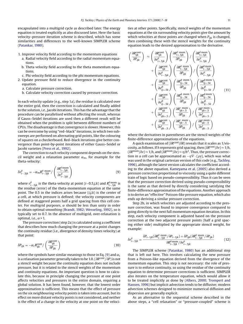
hen combining these with the stencil weights for the continuityquation leads to the desired approximation to the derivative.(
∂Rcontijk
∂Pijk
)≈(
∂Rcontijk
∂vi+.5jk
)(∂R mom
i+.5jk
∂Pijk
)/
(∂R mom
i+.5jk
∂vi+.5jk
)
+(
∂Rcontijk
∂vi−.5jk
)(∂R mom
i−.5jk
∂Pijk
)/
(∂R mom
i−.5jk
∂vi−.5jk
)
+(
∂Rcontijk
∂vij+.5k
)(∂R mom
ij+.5k
∂Pijk
)/
(∂R mom
ij+.5k
∂vij+.5k
)
+(
∂Rcontijk
∂vij−.5k
)(∂R mom
ij−.5k
∂Pijk
)/
(∂R mom
ij−.5k
∂vij−.5k
)
+(
∂Rcontijk
∂vrijk+.5
)(∂Rr mom
ijk+.5
∂Pijk
)/
(∂Rr mom
ijk+.5
∂vrijk+.5
)
+(
∂Rcontijk
∂vrijk−.5
)(∂Rr mom
ijk−.5
∂Pijk
)/
(∂Rr mom
ijk−.5
∂vrijk−.5
)
(11)
here the derivatives in parentheses are the stencil weights of thenite-difference approximations of the equations.
A quick examination of (ıRcont/ıR) reveals that it scales as 1/vis-osity, as follows. If h represents grid spacing, then (ıRcont/ıv) ≈ 1/h,ıRmom/ıv) ≈ 1/h, and (ıRmom/ıv) ≈ �/h2. Thus, the pressure correc-ion in a cell can be approximated as −�∇ · (�v), which was whatas used in the original cartesian version of this code (e.g., Tackley,
996), although the latest version calculates the coefficient accord-ng to the above equation. Kameyama et al. (2005) also derived aressure correction proportional to viscosity using a quite differentrain of logic based on pseudo-compressibility. Thus it can be seenhat the pressure correction derived using pseudo-compressibilitys the same as that derived by directly considering satisfying thenite-difference approximation of the equations. Another approach
s to derive an “effective” Poisson-like pressure equation, which alsonds up deriving a similar pressure correction.
Step 2b, in which velocities are adjusted according to the pres-ure correction, was found to improve convergence compared tooing directly to the next full momentum equation iteration. In thistep, each velocity component is adjusted based on the pressureorrection at the two adjacent pressure points (half a grid spac-ng either side) multiplied by the appropriate stencil weight, forxample:
vi−.5jk =
ıPi−1jk(∂R momi−.5jk
/∂Pi−1jk) + ıPijk(∂R momi−.5jk
/∂Pijk)
∂R momi−.5jk
/∂vi−.5jk
(12)
The SIMPLER scheme (Patankar, 1980) has an additional stephat is left out here. This involves calculating the new pressurerom a Poisson-like equation derived from the divergence of the
omentum equation. This step is not necessary: the role of pres-ure is to enforce continuity, so using the residue of the continuityquation to determine pressure corrections is sufficient. SIMPLERlso iterates on the temperature equation, which would allow ito be treated implicitly as done by (Albers, 2000; Trompert and
ansen, 1996) but implicit advection tends to be diffusive; moderndvection schemes designed to minimize numerical diffusion andispersion are generally explicit.As an alternative to the sequential scheme described in thebove steps, a “cell relaxation” or “pressure-coupled” scheme is
1 nd Pla
ars(iTtnpioV
3
eeoosWgarvigcfirg
dvagtcolflgailt
i(eUmetsbae
mgST
aaspicagl(iiwnci
trbh
3
easf(dmp
opcegctaacpTItcvS
ı
wta
2 P.J. Tackley / Physics of the Earth a
lso implemented, in which corrections to the pressure and six sur-ounding velocities are calculated simultaneously using a matrixolution method, which involves a 7×7 matrix in three dimensionsTackley, 2000a). Using this scheme, the solution converges in fewerterations, but it takes several times as much CPU time per iteration.hus, the overall solution time is longer. Both the point-wise andhe cell-wise schemes appear to be similar in their robustness (oron-robustness) to large viscosity variations, therefore the fasteroint-wise scheme is favoured at present. Auth and Harder (1999)
mplemented a similar scheme in a 2D code except using a diag-nalised version of the matrix instead of the full matrix, based onanka (1986).
.4. Multigrid cycles
The multigrid method, in which the residue (error) to thequations is relaxed on a heirarchy of nested grids with differ-nt grid spacing, can dramatically accelerate the convergence ratef iterative solvers because in principle it relaxes all wavelengthsf the residue simultaneously, resulting in a solution time thatcales in proportion to the number of unknows (Brandt, 1982;
esseling, 1992). For mantle convection this was applied to a stag-ered velocity–pressure grid by Tackley (1993). A key problem withpplying the multigrid method to mantle convection is a lack ofobustness to large viscosity variations, i.e., the iterations convergeery slowly or diverge (e.g., that initial study only reached viscos-ty contrasts of 103). Broadly speaking this is because the coarserids do not “see” correctly the fine-grid problem, so correctionsalculated at coarse levels may actually degrade the solution atner levels rather than improving it. Thus, over the years, severalesearchers have proposed improvements to staggered grid multi-rid algorithm to address this problem.
In the general multigrid literature, the accepted approach toeriving coarse-grid operators, particularly in the case of stronglyarying coefficients, is to use matrix-dependent prolongationnd restriction operators combined with the Galerkin coarse-rid approximation (GCGA) (e.g., Wesseling, 1992). To explain theerminology: the prolongation operator P is used to interpolateoarse-grid corrections to the next finest grid, while the restrictionperator R is used to restrict fine-grid residue to the next coarsestevel. “Matrix-dependent” means that these operators are derivedrom the stencil (matrix) of the discretized equations at the finerevel, e.g., A. In the Galerkin coarse-grid approximation, the coarse-rid operator is based on the fine grid operator and the prolongationnd restriction operators as: Ac = RAfP, the interpretation of whichs that is has the same effect as prolongating the fields to the finerevel, applying the fine-grid operator then restricting the result tohe coarser level.
Matrix-dependent operators and the Galerkin coarse grid weremplemented in a 2D finite-element mantle convection code byYang and Baumgardner, 2000) with apparently astonishing results,asily handling viscosity contrasts of 1010 between adjacent points.nfortunately, similar robustness was not obtained when theethod was implemented in the related 3D spherical shell finite-
lement code TERRA (J. R. Baumgardner, personal communication),he reason for which is uncertain. The method has not yet beenuccessfully applied to a staggered grid mantle convection codeecause of the complexity in this case, although they have beenpplied to the constant viscosity incompressible Navier–Stokesquations (Zeng and Wesseling, 1992a,b).
So far, mantle convection implementations of staggered gridultigrid have instead re-discretized the equations on the coarse
rid using a viscosity field that is averaged from the fine grid.everal authors have proposed improvements to the scheme ofackley (1993). Firstly, Trompert and Hansen (1996) introduced
l
C
netary Interiors 171 (2008) 7–18
new averaging scheme for the coarse-grid viscosities, in whichnisotropic viscosities are used to calculate the coarse-grid sheartresses. They also found that taking additional iterations on theressure term helped overall convergence. Auth and Harder (1999)
ntroduced pressure-coupled relaxations, found that convergencean be greatly improved by using F-cycles instead of V-cycles, andlso found that arithmetic averaging of viscosities to the coarserid gives greater robustness than harmonic averaging and a simi-ar performance to the Trompert and Hansen (1996) scheme. Albers2000) introduced mesh refinement, and also found that robustnesss greatly improved by using multigrid cycles that conduct moreterations on the coarse grids such F-cycles, W-cycles and V-cycles
ith more coarse iterations. Kameyama et al. (2005) introduced aew way of conceptualising the iteration process, namely “pseudo-ompressibility, and again found that taking additional coarse-gridterations greatly improves robustness to large viscosity variations.
Most of these improvements have been tried in Stag3D, withhe result that viscosity contrasts in the range 105 to 106 could beoutinely handled (e.g., Ratcliff et al., 1997; Tackley, 1998a, 2000a),ut this is still much lower than Earth-like. An additional schemeas been implemented in the new version, as described below.
.5. Pressure interpolation scheme
The “standard” transfer operators used in this code are lin-ar interpolation for prolongation and restriction, which includesrithmetic averaging of the viscosity field to the coarse grids, cho-en solely for the reason that it generally gives better convergenceor large viscosity contrasts, as also noted by Auth and Harder1999). Here, it is also not attempted to implement the full matrix-ependent transfers plus GCGA, but rather the philosophy behindatrix-dependent operators is used to propose an improvement to
ressure interpolation.Based on experimentation, it has been found that the main cause
f non-convergence with large viscosity variations in Stag3D isressure corrections passed from coarse to fine grids. The pressureorrection is roughly proportional to local viscosity, as discussedarlier. If a fine grid cell has a much lower viscosity than the coarse-rid cell that contains it, then the prolongated pressure correctionan be much too large, making the fine grid solution worse. Indeed,his is probably why Trompert and Hansen (1996) found that takingdditional pressure iterations is so helpful: the additional iterationsre needed to repair the damage done by the “correction” from theoarser grid. A simple remedy would thus seem to be to adjust theressure corrections by the ratio of fine grid to coarse-grid viscosity.his was found to give improvement in some cases, but not robustly.nstead, it is chosen to adjust the prolongated pressure accordingo the term (∂Rcont/∂P) ≡ (∂(∇ · (�v))/∂P) introduced earlier, whichan be regarded as containing a sort of weighted average of localiscosity values rather than the viscosity at an individual point.pecifically:
Pfine = CıPcoarse
(∂Rcont/∂P)fine(13)
here C is a constant. Noting that in 3D one coarse-grid cell mapso eight fine-grid cells, C is computed using the criterion that theverage pressure must be conserved, i.e.,
18
∑ıPfine = ıPcourse (14)
eading to
= 8
(∑ 1(dRcont/dP)fine
)−1
(15)
nd Pla
Tipltltcvs
osearfawosHme
3
mieeCtc
MscutvtKwTos
3
cmotacwptctii
dte
iocebbnpwd
wbidfiiC
tadcl
3
artantestRao
pc
4
4
a1ildI
P.J. Tackley / Physics of the Earth a
his reduces to simple injection in the case of constant viscos-ty (i.e., eight fine grid pressures are set equal to the coarse-gridressure). This scheme is something like a matrix-dependent pro-
ongation operator for pressure. In matrix-dependent operatorheory, the restriction operator should be the transpose of the pro-ongation operator. Curiously, this was not found to be helpful inhis application. Similar operators have been tried for the velocityomponents, but again did not seem to help significantly. Con-ergence tests comparing the performance of this scheme to thetandard linear interpolation are given later.
It is emphasised that pressure and velocity are treated (iteratedn) together at every multigrid level, and thus a velocity–pressureolution is obtained in a single set of multigrid cycles. This is differ-nt from the common practice in finite-element codes (e.g., Moresind Solomatov, 1995; Zhong et al., 2000), in which multigrid cycleselax only the velocity and separate, outer iterations must be doneor pressure. In that case, several sets of multigrid cycles on velocitylternating with some type of iterations on pressure are required,ith the result that it can take as much as 10 times more CPU time to
btain a velocity–pressure solution, compared with treating themimultaneously as is normally done in codes like StagYY (J. vanunen, personal communication, 2006), although recent imple-entations of the finite-element multigrid method may be more
fficient (S. Zhong, personal communication, 2008).
.6. Advection and energy equation
The energy equation is advanced in time using an explicitethod. Viscous dissipation, diffusion, and adiabatic heat-
ng/cooling are calculated using finite-differences. Latent heatffects due to phase transitions are included in the form of anffective heat capacity and thermal expansivity, as introduced byhristensen and Yuen (1985) (in previous versions these terms werereated by advecting potential temperature, but this has now beenhanged).
Thermal advection is performed using the finite-volumePDATA scheme of (Smolarkiewicz, 1984), which uses a correction
cheme to subtract the numerical diffusion of the upwind donorell method. This scheme is written for a cartesian domain, so tose it without modification in spherical geometry the velocities areransformed into face mass fluxes and a correction is made for cellolume. This scheme can also be used for a non-diffusive composi-ional field in conjunction with the “Lenardic filter” (Lenardic andaula, 1993), a combination that works quite well for stable layersith sharp interfaces (e.g., as tested in Tackley and King (2003)).
racers are advecting using a standard second-order or fourth-rder Runge–Kutta, taking care to include the correction terms forpherical geometry.
.7. Parallelisation
A simple domain decomposition is applied in all three sphericaloordinate directions and the yin and yang blocks. Each subdo-ain contains an extra sheet of “ghost” cells that contain copies
f the cells on the outer part of adjacent subdomains and act ashe boundary condition for the local subdomain, a commonly usedpproach. After a field is updated, these ghost values are communi-ated. Simple-mindedly, it would seem necessary to communicateith up to 26 other nodes in order that edge and corner ghostoints are correctly transferred; this can, however, be accomplished
hrough communication with only six other nodes by using threeonsecutive communication steps in the three orthogonal direc-ions, each with the two nodes that contain adjacent subdomainsn the relevant direction. Tracer particles are held in the subdomainsn which they are present, and are communicated with other sub-gI+tb
netary Interiors 171 (2008) 7–18 13
omains when they cross the boundaries. If a tracer is present inhe overlapping region of the yin-yang grid, then a copy is held inach subgrid.
If a single grid block is being used (cartesian or regional spher-cal) then the communication patterns remain simple regardlessf the number of nodes being used, but this is not the case forommunication between the “yin” grid and the “yang” subgrid. Ifach of these subgrids is split more than four ways (i.e., bisected inoth the theta and phi directions), then communication along theoundary requires each node to communicate with two or moreodes on the other grid. Thus, for simplicity the decomposition isresently limited to a maximum of four ways, resulting in an eight-ay azimuthal decomposition. The grid is also split in the radialirection, typically eight ways so that cases can be run on 64 CPUs.
The multigrid algorithm involves going to very coarse grids, onhich calculations are not efficient in parallel (or there might even
e fewer points than CPUs). Thus, at some point in the coarsen-ng process the calculation is moved to a single CPU (or actually,uplicated on all CPUs), and then split again during the coarse-to-ne process. With a relatively small number of CPUs like 64, this
s done only for the very coarsest grid. A future expansion to morePUs might require introducing intermediate steps in this process.
The code is parallelised for distributed memory computers usinghe MPI message-passing library, although it may also be run on
machine without MPI installed by linking to a file containingummy MPI calls. The code is written as a stand-alone code thatan be run on any computer with a Fortran 95 compiler, with noibraries required.
.8. Rigid body rotation
In a spherical shell with free slip upper and lower bound-ries, the solution is undetermined to an arbitrary net (rigid body)otation. Although this has not been found to be a problem for short-erm calculations, over many timesteps net rotation can built upnd create problems. Thus, at every timestep the code calculates theet rotation relative to three orthogonal axes and subtracts it fromhe solution. This net rotation calculation can be done either for thentire volume, or for just the outermost layer. These do not neces-arily produce the same answer because there are good reasons forhe interior to display net rotation relative to the lithosphere (e.g.,icard et al., 1991). In order to make it easier to analyse rigid lidsnd plate tectonics, the usual choice is to subtract the net rotationf the outermost layer.
In a cartesian domain, such a concern also applies in the case oferiodic side boundaries. In this case, the mean horizontal flow isalculated and subtracted at every timestep.
. Results
.1. Parallel performance
The performance and scaling of StagYY on up to 64 CPUs ofBeowulf cluster with resolutions from 25 million to more thanbillion unknowns is shown in Fig. 2. The number of unknowns
s four times the number of grid points. For this test, the Gonza-es cluster at ETH was used, which consists of nodes containingual AMD Opteron 250 CPUs connected with a Quadrics QsNet
I interconnect. Fig. 2 (top row) shows the time taken per multi-
rid F-cycle. In Fig. 2a, perfect scaling would be a line of slope −1.n Fig. 2b, perfect scaling would be a straight line with a slope of1. These graphs indicate that the time is roughly proportional tohe number of unknowns and inversely proportional to the num-er of CPUs, as hoped for. One F-cycle with 1.2 billion unknowns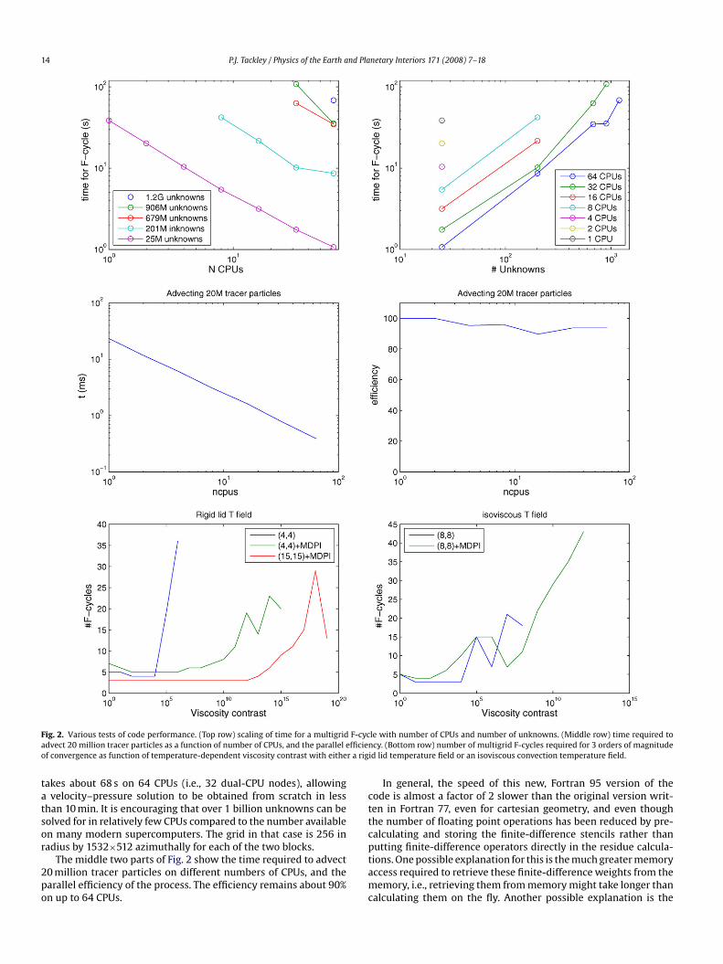
14 P.J. Tackley / Physics of the Earth and Planetary Interiors 171 (2008) 7–18
F F-cyca fficieno r a rig
tatsor
2po
cttc
ig. 2. Various tests of code performance. (Top row) scaling of time for a multigriddvect 20 million tracer particles as a function of number of CPUs, and the parallel ef convergence as function of temperature-dependent viscosity contrast with eithe
akes about 68 s on 64 CPUs (i.e., 32 dual-CPU nodes), allowingvelocity–pressure solution to be obtained from scratch in less
han 10 min. It is encouraging that over 1 billion unknowns can beolved for in relatively few CPUs compared to the number availablen many modern supercomputers. The grid in that case is 256 in
adius by 1532×512 azimuthally for each of the two blocks.The middle two parts of Fig. 2 show the time required to advect0 million tracer particles on different numbers of CPUs, and thearallel efficiency of the process. The efficiency remains about 90%n up to 64 CPUs.
ptamc
le with number of CPUs and number of unknowns. (Middle row) time required tocy. (Bottom row) number of multigrid F-cycles required for 3 orders of magnitude
id lid temperature field or an isoviscous convection temperature field.
In general, the speed of this new, Fortran 95 version of theode is almost a factor of 2 slower than the original version writ-en in Fortran 77, even for cartesian geometry, and even thoughhe number of floating point operations has been reduced by pre-alculating and storing the finite-difference stencils rather than
utting finite-difference operators directly in the residue calcula-ions. One possible explanation for this is the much greater memoryccess required to retrieve these finite-difference weights from theemory, i.e., retrieving them from memory might take longer thanalculating them on the fly. Another possible explanation is the
nd Pla
uwsip
4
yitwpuitmflwttcttetcvioIpcit
ttnucodKa
aoctosrim
gbnctvn
ewWna
tttbitl
4
spdtaaFlvT2woolpadttia
rBmno(ateTt
tSmstmTn
P.J. Tackley / Physics of the Earth a
se of Fortran 95 dynamically allocated arrays and defined types,hereas the original version was written in Fortran 77 with much
impler data structures such as compiled-in array sizes. More works needed to determine this and optimise the single-CPU floating-oint performance of the latest version.
.2. Multigrid convergence
In general, the multigrid convergence obtained with the yin-ang grid is not as good as that obtained in a single spherical block orn cartesian geometry. Plotting the location of the residue indicateshat this is due to the interface between the two subgrids. Furtherork is needed to understand and improve this situation, but theresent convergence is certainly rapid enough for the code to be aseful scientific tool. As with previous studies discussed earlier, it
s found that F-cycles give better convergence than V-cycles, andhat additional iterations at coarse levels further enhance perfor-
ance. Thus, the standard iteration parameters are F-cycles withour times as many iterations at the coarse levels as at the finestevel, plus various points discussed earlier: red–black iterations
ith ˛m = 0.7 and ˛c = 1.0, geometrical interpolation of viscosityo the shear stress points and arithmetic averaging of viscosityo coarse grids. Note that it is fine to use a different average foroarse-grid viscosity because coarse-grid corrections do not affecthe accuracy of the final solution, only the convergence rate towardshat solution. All averaging or interplation is thus done using a lin-ar (arithmetic) method, except for the interpolation of viscosity onhe same grid level, which is geometric. Another point is that whenalculating the rms. residue, residues are normalised by the localiscosity as represented by the stencil weight. The effect of thiss to measure the error in absolute velocity, otherwise in regionsf high viscosity small velocity variations give enormous residues.n the case of non-convergence, the code includes an automatedrocess that reduces the fraction of the prolongated coarse-gridorrection that is applied to the fine grid, which often helps butndicates the need for optimal prolongation and restriction opera-ors.
Fig. 2 (bottom row) shows the number of F-cycles neededo reduce the residue to 10−3 of its initial value, as a func-ion of viscosity contrast and the iteration parameters such asumber of iterations at each level. Two initial conditions aresed: rigid lid convection with a viscosity contrast of 106, andonstant-viscosity convection. Of particular interest is the effectf the “matrix-dependent” pressure-interpolation (MDPI) schemeescribed above. Similar plots were made by Albers (2000) andameyama et al. (2005) to show the effect of various smoothersnd multigrid cycles.
Using the rigid lid T field, F-cycles with four smoothing iter-tions at each step and no MDPI are able to handle a maximumf 6 orders of magnitude viscosity contrast, with the number of F-ycles increasing rapidly above 4 orders of magnitude. Switching onhe MDPI scheme increases the maximum viscosity contrast to 15rders of magnitude, with the required number of cycles increasingignificantly only above about 10 orders of magnitude. Additionalobustness can be obtained by increasing the number of smoothingterations at each level, for example with 15 iterations the maxi-
um viscosity contrast increases to 19 orders of magnitude.With this rigid lid T field, most of the viscosity contrast occurs
radually over the conductive lid, such that the maximum contrastetween adjacent points is a factor 54,000 with 19 orders of mag-
itude global contrast. Starting from an isoviscous T field is morehallenging because the large temperature hence viscosity con-rasts occur over very short lengthscales; this is an “unrealistic”iscosity field but useful for testing purposes. Thus, it was foundecessary to increase the number of smoothing iterations to eight atm
RpT
netary Interiors 171 (2008) 7–18 15
ach level to get reasonable convergence (Fig. 2 bottom right), andith this up to 8 orders of magnitude were possible without MDPI.ith MDPI this increases to 12 orders of magnitude but a large
umber of F-cycles is necessary. In that case the contrast betweendjacent points is as much as 196,000.
The main conclusion is thus that MDPI can dramatically improvehe robustness to large viscosity variations. Of course, this refers tohe convergence of the numerical scheme to the discretized solu-ion, not the accuracy of the discretized solution, which needs toe tested separately. At low viscosity contrasts MDPI sometimes
ncreases the needed number of F-cycles: this is probably becausehe interpolation scheme is lower order, i.e., injection rather thaninear.
.3. Benchmark tests
Extensive testing and benchmarking of Stag3D in carte-ian geometry has been performed and reported in previousublications. For thermal convection with constant or temperature-ependent viscosity, Stag3D can successfully reproduce thewo-dimensional benchmark cases in Blankenbach et al. (1989)nd three-dimensional benchmark cases in Busse et al. (1994),s detailed in Tackley (1994) and summarized in Tackley (1996).or cases with self-consistently generated plate tectonics, in whicharge viscosity contrasts occur over very short lengthscales, a con-ergence test was presented in the Appendix of Tackley (2000b).his test showed the effect of resolution, varying in factors offrom 16 × 16 × 4 to 256 × 256 × 64, on the outcome of a caseith self-consistent plates. Remarkably, plate-like behaviour was
btained with all resolutions above 32 × 32 × 8, but at lower res-lutions the weak zones (“plate boundaries”) tend to follow gridines. For thermo-chemical convection, Tackley and King (2003)resented benchmark tests and convergence tests for both Stag3Dnd the finite-element code ConMan (King et al., 1990). Theseemonstrated that Stag3D can reproduce the earlier benchmarkests of van Keken et al. (1997), and compared convergence tests forracer-based and grid-based methods of representing compositionn thermo-chemical convection, determining the needed resolutionnd number of tracers.
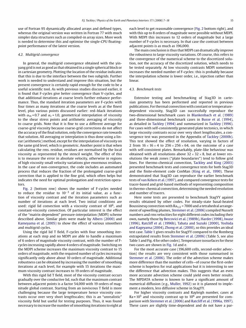
Here some tests are presented to benchmark StagYY againstesults obtained by other codes. For steady-state basal-heatedoussinesq convection with Ra1/2 = 7000 and a tetrahedral arrange-ent of upwelling plumes, Stemmer et al. (2006) compiled Nusselt
umbers and rms velocities for eight different codes including theirwn, namely those by Bercovici et al. (1989b), Harder (1998), Iwase1996), Ratcliff et al. (1996b), Tabata and Suzuki (2000), Yoshidand Kageyama (2004), Zhong et al. (2000), so this provides an idealest case. Table 1 gives results for StagYY compared to the Rombergxtrapolated results from Stemmer et al. (2006) (Table 5, see alsoable 1 and Fig. 4 for other codes). Temperature isosurfaces for thesewo cases are shown in Fig. 1d and e.
For the most accurate case (196,600 cells, second-order advec-ion) the results are very consistent with those summarised intemmer et al. (2006). The order of the advection scheme makesore difference than the number of cells—of course the first-order
cheme is hopeless for real applications but it is interesting to seehe difference that advection makes. This suggests that an even
ore accurate advection scheme could yield even better results.he MPDATA scheme is known to have a significant amount ofumerical diffusion (e.g., Muller, 1992) so it is planned to imple-
ent a modern, less diffusive scheme in StagYY.For higher viscosity contrasts and Rayleigh number, cases ata = 105 and viscosity contrast up to 106 are presented for com-arison with Stemmer et al. (2006) and Ratcliff et al. (1996a, 1997).hese cases are slightly time-dependent and do not have a par-
16 P.J. Tackley / Physics of the Earth and Planetary Interiors 171 (2008) 7–18
Table 1StagYY results for the tetrahedral pattern at Ra = 7000, isoviscous or viscosity contrast 20
nr, nt, np, nb # Cells Adv. order �� = 1:Nu v �� = 20:Nu v
16 × 16 × 48 × 2 24,576 1 3.62 32.87 3.26 25.612 3.49 32.40 3.13 25.51
32 × 32 × 96 × 2 196,608 1 3.57 32.98 3.22 25.852 3.
Stemmer et al. Extrapolated 3.
The last row lists the results from Stemmer et al. (2006) Table 5 which use a Romberg ext
Table 2Basally heated cases with Ra1/2 = 105 and viscosity contrast up to 106
�� Nu v
1 7.27 160.211
T
trtbi
pTpiatccdp
4
pFre(ppp
iiepsH
5
astyec1
tprigtpsl
cspr1ttsiul
wtmtt
FstfisoSgsu
A
tD
R
A
A
03 6.06 96.806 6.50 40.4
hese are with 196,608 cells as listed above and second order advection.
icular symmetry. They are started from a conductive profile withandom perturbations. Due to the random nature, the resulting pat-ern is not expected to exactly match previously published cases,ut the results are within the range of previous results, as illustrated
n Fig. 1g–i and Table 2.For a more complex scenario including compressibility and a
hase transition, an attempt is made to reproduce the result ofackley et al. (1993). The present reference state uses a differentarameterisation but is tuned to match depth profiles of phys-
cal properties as closely as possible. The results (Fig. 1f) showgood resemblance, with the upper mantle containing linear,
ime-dependent downwellings and the lower mantle containingylindrical “avalanches”. It is reassuring that two codes usingompletely different numerical methods (spectral versus finite-ifference) are able to obtain similar results with relatively complexhysics.
.4. Other example results
Scientific findings using StagYY are being detailed in otherapers; here a few sample results are included for illustration.ig. 1j–l shows a thermo-chemical, multiple phase transition caseeported fully in Nakagawa and Tackley (2008). This case uses trac-rs to represent the compositional field, using the ratio methodTackley and King, 2003). Chemically dense material is swept intoiles in upwelling regions, and the locations where the post-erovskite phase are present (Fig. 1l) are anticorrelated with theseiles.
Self-consistent generation of plate tectonics has been a majornterest in the field, so Fig. 1m–o reproduces a case similar to thosen Tackley (2000a,b) except in spherical rather than cartesian geom-try. In these cases, plastic yielding breaks the rigid lid. For thisarticular parameter combination a novel platform is found con-isting of an approximately great circle downwelling (Fig. 1o) (vaneck and Tackley, in press).
. Discussion and future directions
This paper documents how the use of the yin-yang grid hasllowed an existing cartesian code, Stag3D (Tackley, 1993), to betraightforwardly converted to model a 3D spherical shell. Although
here are now two other mantle convection codes that use the yin-ang grid (those of Yoshida and Kageyama (2004) and Kameyamat al., 2008), the one reported here is the latest evolution of aode that has been in continuous use and development for over4 years so has more features and implemented physics. ComparedB
B
48 32.57 3.15 25.714949 32.6234 3.1526 25.76
rapolation of results at increasing resolutions.
o the code of Yoshida and Kageyama (2004) these include com-ressibility, phase transitions, compositional variations, non-linearheology, parallelisation, tracers to track composition, and the abil-ty to model spherical patches, cartesian boxes, and various 2Deometries by changing one input switch. Tests presented showhat StagYY produces results that are consistent with previouslyublished results, and so it is being used to perform new scientifictudies. StagYY is designed to be a stand-alone application with noibraries required, but if MPI is present it can be run in parallel.
Convergence of a multigrid solver in the presence of realisti-ally large viscosity variations has always been a problem withuch codes, as discussed earlier. In this paper a new pressure inter-olation scheme is presented that can dramatically improve theobustness of the iterations to large viscosity variations, with up to9 orders of magnitude variation in the presented tests. One goal forhe future is to further investigate such prolongation and restric-ion schemes in an attempt to arrive at a perfectly robust solutioncheme. Use of the Galerkin coarse-grid approximation may be anngredient to such a scheme. A related promising technology is these of algebraic multigrid, which is designed to overcome several
imitations of geometric multigrid as used here.Another goal for the future is to implement grid refinement,
hich is straightforwardly treated in multigrid schemes by goingo finer grid levels in some areas than in others, as illustrated for
antle convection by Albers (2000). This could be fixed, e.g., withhe upper mantle being better resolved than the lower mantle andhe lithosphere being better resolved still, or adaptive.
Some technical issues remain regarding code performance.irstly, StagYY is around a factor of two slower than the old ver-ion (Stag3D) even in cartesian geometry, which could be dueo the higher memory bandwidth required due to the storage ofnite-difference weights in memory, or due to more complex datatructures made possible by Fortran 95. Investigation and remedyf this should allow substantial performance gains to be realized.econdly, multigrid cycles converge more slowly with the yin-yangrid than with a single spherical or cartesian block, with the edgesomehow slowing things down. Nevertheless, the code is already aseful tool for investigating mantle processes.
cknowledgements
The author thanks Takashi Nakagawa and Hein van Heck forheir images, and Masanori Kameyama, Guillaume Richard andani Schmid for constructive reviews.
eferences
lbers, M., 2000. A local mesh refinement multigrid method for 3-D convectionproblems with strongly variable viscosity. J. Comput. Phys. 160 (1), 126–150.
uth, C., Harder, H., 1999. Multigrid solution of convection problems with strongly
variable viscosity. Geophys. J. Int. 137 (3), 793–804.alachandar, S., Yuen, D.A., Reuteler, D.M., 1996. High Rayleigh number convec-tion at infinite Prandtl number with weakly temperature-dependent viscosity.Geophys. Astrophys. Fluid Dyn. 83 (1–2), 79–117.
aumgardner, J.R., 1985. 3-dimensional treatment of convective flow in the earthsmantle. J. Stat. Phys. 39 (5–6), 501–511.
nd Pla
B
B
B
B
BB
C
C
C
C
D
G
G
H
H
H
H
H
I
K
K
K
K
L
M
M
M
M
N
N
O
P
P
R
R
R
R
R
R
S
S
S
S
T
T
T
T
T
T
T
T
T
T
T
T
T
T
v
v
V
W
X
P.J. Tackley / Physics of the Earth a
aumgardner, J.R., 1988. Application of supercomputers to 3-D mantle convection.In: Runcorn, S.K. (Ed.), The Physics of the Planets. Wiley, New York, pp. 199–231.
ercovici, D., Schubert, G., Glatzmaier, G.A., 1989a. 3-dimensional spherical-modelsof convection in the earths mantle. Science 244 (4907),950–955.
ercovici, D., Schubert, G., Glatzmaier, G.A., Zebib, A., 1989b. 3-dimensional thermal-convection in a spherical-shell. J. Fluid Mech. 206 (Sep.), 75–104.
lankenbach, B., et al., 1989. A benchmark comparison for mantle convection codes.Geophys. J. Int. 98 (1), 23–38.
randt, A., 1982. Guide to multigrid development. Lect. Notes Math. 960,220–312.usse, F.H., et al., 1994. 3D convection at infinite Prandtl number in Carte-
sian geometry—a benchmark comparison. Geophys. Astrophys. Fluid Dyn. 75(1),39–59.
hoblet, G., 2005. Modelling thermal convection with large viscosity gradients inone block of the ‘cubed sphere’. J. Comput. Phys. 205 (1), 269–291.
hristensen, U., Harder, H., 1991. 3-D convection with variable viscosity. Geophys. J.Int. 104 (1), 213–226.
hristensen, U.R., Yuen, D.A., 1985. Layered convection induced by phase transitions.J. Geophys. Res. 90 (B12), 10291–10300.
onnolly, J.A.D., 2005. Computation of phase equilibria by linear programming: a toolfor geodynamic modeling and an application to subduction zone decarbonation.Earth Planet. Sci. Lett. 236, 524–541.
eubelbeiss, Y., Kaus, B.J.P., 2008. A comparison of Eulerian and Lagrangian numer-ical techniques for the Stokes equation in the presence of strongly varyingviscosity. Phys. Earth Planet. Int. 171, 92–111.
erya, T.V., Connolly, J.A.D., Yuen, D.A., Gorczyk, W., Capel, A.M., 2006. Seismic impli-cations of mantle wedge plumes. Phys. Earth Planet. Int. 156, 59–74.
latzmaier, G.A., 1988. Numerical simulations of mantle convection—time-dependent, 3-dimensional, compressible, spherical-shell. Geophys. Astrophys.Fluid Dyn. 43 (2), 223–264.
arder, H., 1998. Phase transitions and the three-dimensional planform of thermalconvection in the Martian mantle. J. Geophys. Res. 103 (E7), 16775–16797.
arder, H., Christensen, U.R., 1996. A one-plume model of martian mantle convec-tion. Nature 380 (6574), 507–509.
arder, H., Hansen, U., 2005. A finite-volume solution method of thermal convectionand dynamo problems in spherical shells. Geophys. J. Int. 161, 522–532.
ernlund, J.W., Tackley, P.J., 2008. Modeling mantle convection in the sphericalannulus. Phys. Earth Planet. Int. 171, 48–54.
ernlund, J.W., Tackley, P.J., 2003. Three-dimensional spherical shell convection atinfinite Prandtl number using the ‘cubed sphere’ method, Second MIT Confer-ence on Computational Fluid and Solid Mechanics. Elsevier, MIT.
wase, Y., 1996. Three-dimensional infinite Prandtl-number convection in a spher-ical shell with temperature-dependent viscosity. J. Geomag. Geoelectr. 48,1499–1514.
ageyama, A., Sato, T., 2004. The “yin-yang grid”: an overset grid in spherical geom-etry. Geochem. Geophys. Geosyst. 5(Q09005): doi:10.1029/2004GC000734.
ameyama, M., Kageyama, A., Sato, T., 2005. Multigrid iterative algorithm usingpseudo-compressibility for three-dimensional mantle convection with stronglyvariable viscosity. J. Comput. Phys. 206, 162–181.
ameyama, M., Kageyama, A., Sato, T., 2008. Multigrid-based simulation code formantle convection in spherical shell using Yin–Yang grid. Phys. Earth Planet. Int.171, 19–32.
ing, S.D., Raefsky, A., Hager, B.H., 1990. Conman—vectorizing a finite-element codefor incompressible 2-dimensional convection in the earths mantle. Phys. EarthPlanet. Inter. 59 (3), 195–207.
enardic, A., Kaula, W.M., 1993. A numerical treatment of geodynamic viscous-flowproblems involving the advection of material interfaces. J. Geophys. Res. SolidEarth 98 (B5), 8243–8260.
achetel, P., Thoraval, C., Brunet, D., 1995. Spectral and geophysical consequencesof 3-D spherical mantle convection with an endothermic phase-change at the670 km discontinuity. Phys. Earth Planet. Inter. 88 (1), 43–51.
onnereau, M., Quere, S., 2001. Spherical shell models of mantle convection withtectonic plates. Earth Planet. Sci. Lett. 184, 575–587.
oresi, L.N., Solomatov, V.S., 1995. Numerical investigation of 2D convection withextremely large viscosity variations. Phys. Fluids 7 (9), 2154–2162.
uller, R., 1992. The performance of classical versus modern finite-volume advec-tion schemes for atmospheric modeling in a one-dimensional test-bed. Mon.Weather Rev. 120 (7), 1407–1415.
akagawa, T., Tackley, P.J., 2005. Three-dimensional numerical simulations ofthermo-chemical multiphase convection in Earth’s mantle. In: Proceedings ofthe Third MIT Conference on Computational Fluid and Solid Mechanics.
akagawa, T., Tackley, P.J., 2008. Lateral variations in CMB heat flux and deep man-tle seismic velocity caused by a thermal-chemical-phase boundary layer in 3Dspherical convection. Earth Planet. Sci. Lett. 271, 348–358.
gawa, M., Schubert, G., Zebib, A., 1991. Numerical simulations of 3-dimensionalthermal convection in a fluid with strongly temperature-dependent viscosity. J.Fluid Mech. 233, 299–328.
atankar, S.V., 1980. Numerical Heat Transfer and Fluid Flow. Hemisphere PublishingCorporation, New York.
ress, W.H., Teulolsky, S.A., Vetterling, W.T., Flannery, B.P., 1992. Numerical Recipes.
Cambridge University Press, Cambridge, UK.atcliff, J.T., Schubert, G., Zebib, A., 1995. 3-dimensional variable viscosity convectionof an infinite Prandtl number Boussinesq fluid in a spherical-shell. Geophys. Res.Lett. 22 (16), 2227–2230.
atcliff, J.T., Schubert, G., Zebib, A., 1996a. Effects of temperature-dependent viscos-ity on thermal convection in a spherical shell. Phys. D 97 (1–3),242–252.
Y
Y
netary Interiors 171 (2008) 7–18 17
atcliff, J.T., Schubert, G., Zebib, A., 1996b. Steady tetrahedral and cubic patterns ofspherical-shell convection with temperature-dependent viscosity. J. Geophys.Res. Solid Earth 101 (B11), 25473–25484.
atcliff, J.T., Tackley, P.J., Schubert, G., Zebib, A., 1997. Transitions in thermalconvection with strongly variable viscosity. Phys. Earth Planet. Inter. 102,201–212.
icard, Y., Doglioni, C., Sabadini, R., 1991. Differential rotation between lithosphereand mantle—a consequence of lateral mantle viscosity variations. J. Geophys.Res. Solid Earth Planets 96 (B5), 8407–8415.
onchi, C., Iacono, R., Paolucci, P.S., 1996. The “cubed sphere”: a new method for thesolution of partial differential equations in spherical geometry. J. Comput. Phys.124 (1), 93–114.
chmeling, H., Babeyko, A.Y., Enns, A., Faccenna, C., Funiciello, F., Gerya, T., Golabek,G.J., Grigull, S., Kaus, B.J.P., Morra, G., Schmalholz, S.M., van Hunen, J., 2008.A benchmark comparison of spontaneous subduction models—towards a freesurface. Phys. Earth Planet. Inter. 171, 198–223.
chubert, G., Turcotte, D.L., Olson, P., 2000. Mantle Convection in the Earth andPlanets. Cambridge University Press.
molarkiewicz, P.K., 1984. A fully multidimensional positive definite advectiontransport algorithm with small implicit diffusion. J. Comput. Phys. 54 (2),325–362.
temmer, K., Harder, H., Hansen, U., 2006. A new method to simulate convectionwith strongly temperature- and pressure-dependent viscosity in a sphericalshell: applications to the Earth’s mantle. Phys. Earth Planet. Inter. 157 (3–4),223–249.
abata, M., Suzuki, A., 2000. A stabilized finite element method for theRayleigh–Benard equations with infinite Prandtl number in a spherical shell.Comput. Methods Appl. Mech. Eng. 190, 387–402.
ackley, P.J., 1993. Effects of strongly temperature-dependent viscosity on time-dependent, 3-dimensional models of mantle convection. Geophys. Res. Lett. 20(20), 2187–2190.
ackley, P.J., 1994. Three-dimensional models of mantle convection: influence ofphase transitions and temperature-dependent viscosity. Ph.D. Thesis. CaliforniaInstitute of Technology, Pasadena, 299 pp.
ackley, P.J., 1996. Effects of strongly variable viscosity on three-dimensionalcompressible convection in planetary mantles. J. Geophys. Res. 101,3311–3332.
ackley, P.J., 1998a. Self-consistent generation of tectonic plates in three-dimensional mantle convection. Earth Planet. Sci. Lett. 157, 9–22.
ackley, P.J., 1998b. Three-dimensional simulations of mantle convection with a ther-mochemical CMB boundary layer: D? In: Gurnis, M., Wysession, M.E., Knittle, E.,Buffett, B.A. (Eds.), The Core-Mantle Boundary Region. Geodynamics. AmericanGeophysical Union, pp. 231–253.
ackley, P.J., 2000a. Self-consistent generation of tectonic plates in time-dependent,three-dimensional mantle convection simulations. Part 1. Pseudo-plastic yield-ing. Geochem., Geophys., Geosys. Volume 1, Paper number 2000GC000036[14,503 words, 21 figures, 1 table].
ackley, P.J., 2000b. Self-consistent generation of tectonic plates in time-dependent,three-dimensional mantle convection simulations. Part 2. Strain weakeningand asthenosphere. Geochem., Geophys., Geosys. Volume 1: Paper number2000GC000043 [14,420 words, 15 figures, 1 table].
ackley, P.J., 2002. Strong heterogeneity caused by deep mantle layering. Geochem.Geophys. Geosys. 3(4), doi:10.1029/2001GC000167.
ackley, P.J., King, S.D., 2003. Testing the tracer ratio method for modeling active com-positional fields in mantle convection simulations. Geochem. Geophys. Geosyst.4(4), doi:10.1029/2001GC000214.
ackley, P.J., Stevenson, D.J., Glatzmaier, G.A., Schubert, G., 1993. Effects of anendothermic phase transition at 670 km depth in a spherical model of convectionin the Earth’s mantle. Nature 361 (6414), 699–704.
ackley, P.J., Stevenson, D.J., Glatzmaier, G.A., Schubert, G., 1994. Effects of multiplephase transitions in a 3-dimensional spherical model of convection in Earth’smantle. J. Geophys. Res. 99 (B8), 15877–15901.
ackley, P.J., Xie, S., 2003. Stag3D: a code for modeling thermo-chemical multiphaseconvection in Earth’s mantle. In: Second MIT Conference on Computational Fluidand Solid Mechanics, Elsevier, MIT, pp. 1–5.
rompert, R.A., Hansen, U., 1996. The application of a finite-volume multigridmethod to 3-dimensional flow problems in a highly viscous fluid with a variableviscosity. Geophys. Astrophys. Fluid Dyn. 83 (3–4), 261–291.
an Heck, H., Tackley, P.J., Planforms of self-consistently generated plate tectonics in3-D spherical geometry, Geophys. Res. Lett., in press.
an Keken, P.E., King, S.D., Schmeling, H., Christensen, U.R., Neumeister, D., Doin, M.P.,1997. A comparison of methods for the modeling of thermochemical convection.J. Geophys. Res. 102 (B10), 22477–22495.
anka, S.P., 1986. Block implicit multigrid solution of Navier–Stokes equations withprimitive variables. J. Comput. Phys. 65, 138–158.
esseling, P., 1992. An Introduction to Multigrid Methods. John Wiley and Sons, 284pp.
ie, S., Tackley, P.J., 2004. Evolution of helium and argon isotopes in a convectingmantle. Phys. Earth Planet. Inter. 146 (3–4), 417–439.
ang, W.-S., Baumgardner, J.R., 2000. A matrix-dependent transfer multigrid methodfor strongly variable viscosity infinite Prandtl number thermal convection. Geo-phys. Astrophys. Fluid Dyn. 92, 151–195.
oshida, M., Iwase, Y., Honda, S., 1999. Generation of plumes under a localizedhigh viscosity lid in 3-D spherical shell convection. Geophys. Res. Lett. 26 (7),947–950.
1 nd Pla
Y
Y
Y
Z
Z
Z
8 P.J. Tackley / Physics of the Earth a
oshida, M., Kageyama, A., 2004. Application of the yin-yang grid to a thermal con-vection of a Boussinesq fluid with infinite Prandtl number in a three-dimensionalspherical shell. Geophys. Res. Lett. 31(L12609), doi:10.1029/2004GL019970.
oshida, M., Kageyama, A., 2006. Low-degree mantle convection with stronglytemperature- and depth-dependent viscosity in a three-dimensional sphericalshell. J. Geophys. Res. 111(B03412), doi:10.1029/2005JB003905.
oung, R.E., 1974. Finite-amplitude thermal convection in a spherical shell. J. FluidMech. 63, 695–721.
eng, S., Wesseling, P., 1992a. An efficient algorithm for the computation ofGalerkin coarse-grid approximation for the incompressible Navier–Stokes equa-tions, Faculty of Technical Mathematics and Informatics, Delft University ofTechnology.
Z
Z
netary Interiors 171 (2008) 7–18
eng, S., Wesseling, P., 1992b. Galerkin coarse grid approximation for the incom-pressible Navier–Stokes equations in general coordinates, Faculty of TechnicalMathematics and Informatics, Delft University of Technology.
hang, S.X., Christensen, U., 1993. Some effects of lateral viscosity variations on geoidand surface velocities induced by density anomalies in the mantle. Geophys. J.Int. 114 (3), 531–547.
hang, S.X., Yuen, D.A., 1996. Various influences on plumes and dynamics in time-dependent compressible mantle convection in 3-D spherical-shell. Phys. EarthPlanet. Inter. 94 (3–4), 241–267.
hong, S., Zuber, M.T., Moresi, L., Gurnis, M., 2000. Role of temperature-dependentviscosity and surface plates in spherical shell models of mantle convection. J.Geophys. Res. 105 (B5), 11063–11082.