Embed Size (px)
Citation preview
Fuzzy-logic based trend classification for fault diagnosis of chemicalprocesses
Sourabh Dash a, Raghunathan Rengaswamy b,*, Venkat Venkatasubramanian a,*a School of Chemical Engineering, Purdue University, West Lafayette, IN 47907, USA
b Department of Chemical Engineering, Clarkson University, Potsdam, NY 13699-5705, USA
Received 10 November 2001; accepted 10 September 2002
Abstract
In this paper, fault diagnosis based on patterns exhibited in the sensors measuring the process variables is considered. The
temporal patterns that a process event leaves on the measured sensors, called event signatures, can be utilized to infer the state of
operation using a pattern-matching approach. However, the qualitative nature of the features leads to imprecise classification
boundaries at the trend-identification stage and hence at the trend-matching stage. Moreover, noise and other underlying
phenomena may lead to non-reproducibility of the same trends chosen to represent an event. Thus, a crisp inference process might
lead to a large knowledge-base of signatures; it could also cause misclassification. To overcome this, a fuzzy-reasoning approach is
proposed to ensure robustness to the inherent uncertainty in the identified trends and to provide succinct mapping. A two-staged
strategy is employed: (i) identifying the most likely fault candidates based on a similarity measure between the observed trends and
the event-signatures in the knowledge-base and, (ii) estimation of the fault magnitude. The fuzzy-knowledge-base consists of a set of
physically interpretable if�/then rules providing physical insight into the process. The technique provides multivariate inferencing
and is transparent. We illustrate the application of the proposed approach in the fault diagnosis of an exothermic reactor case study.
# 2002 Published by Elsevier Science Ltd.
Keywords: Process monitoring; Qualitative trend analysis; Fuzzy logic; Classification; Fault diagnosis
1. Introduction
One of the important reasons for developing a trend
analysis technique is the subsequent use of the classified
trends in fault diagnosis. Hence, typical reasoning
systems that depend on the use of ‘event signatures’
for fault diagnosis have three important components: (i)
A language to represent the trends (ii) A technique to
identify the trends and (3) A mapping from trends to
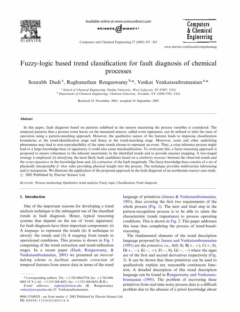
operational conditions. This process is shown in Fig. 1
comprising of the trend extraction and trend-utilization
stages. In a recent paper (Dash, Rengaswamy, &
Venkatasubramanian, 2001) we presented an interval-
halving scheme to facilitate automatic extraction of
temporal features from sensor data in terms of the trend
language of primitives (Janusz & Venkatasubramanian,
1991), thus covering the first two requirements of the
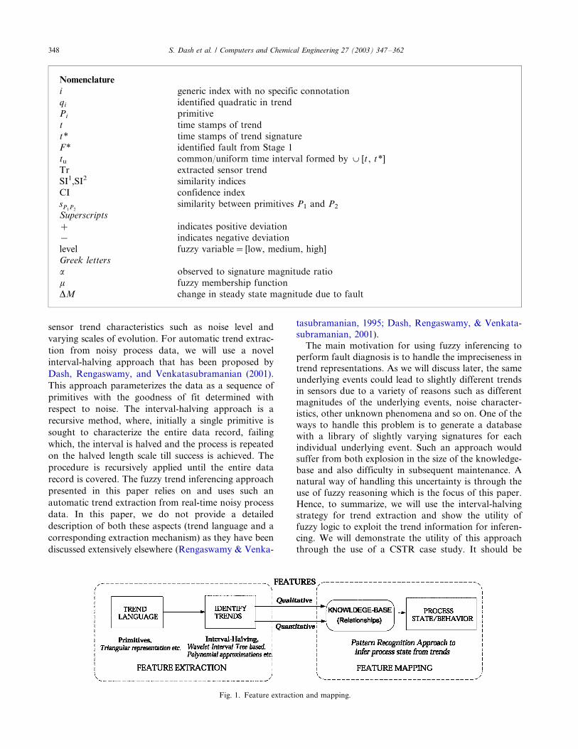
whole process (Fig. 1). The next and final step in the
pattern-recognition process is to be able to relate the
characteristic trends (signatures) to process operating
conditions. This is shown in Fig. 2. This paper addresses
this issue thus completing the process of trend-based-
reasoning.
The fundamental elements of the trend description
language proposed by Janusz and Venkatasubramanian
(1991) are the primitives i.e., A(0, 0), B(�/, �/), C(�/, 0),
D(�/, �/), E(�/, �/), F(�/, 0), G(�/, �/) where the signs
are of the first and second derivatives respectively (Fig.
3). It can be shown that these primitives can be used to
qualitatively explain any reasonable continuous func-
tion. A detailed description of this trend description
language can be found in Rengaswamy and Venkatasu-
bramanian (1995). The problem of recovering these
primitives from real-time noisy process data is a difficult
problem due to the absence of a priori knowledge about
* Corresponding authors. Tel.: �/1-765-494-0734; fax: �/1-765-494-
0805 (V.V.); tel.: �/1-315-268-4423; fax: �/1-315-268-6654 (R.R.).
E-mail addresses: [email protected] (R. Rengaswamy),
[email protected] (V. Venkatasubramanian).
Computers and Chemical Engineering 27 (2003) 347�/362
www.elsevier.com/locate/compchemeng
0098-1354/02/$ - see front matter # 2002 Published by Elsevier Science Ltd.
PII: S 0 0 9 8 - 1 3 5 4 ( 0 2 ) 0 0 2 1 4 - 4
sensor trend characteristics such as noise level and
varying scales of evolution. For automatic trend extrac-
tion from noisy process data, we will use a novel
interval-halving approach that has been proposed by
Dash, Rengaswamy, and Venkatasubramanian (2001).
This approach parameterizes the data as a sequence of
primitives with the goodness of fit determined with
respect to noise. The interval-halving approach is a
recursive method, where, initially a single primitive is
sought to characterize the entire data record, failing
which, the interval is halved and the process is repeated
on the halved length scale till success is achieved. The
procedure is recursively applied until the entire data
record is covered. The fuzzy trend inferencing approach
presented in this paper relies on and uses such an
automatic trend extraction from real-time noisy process
data. In this paper, we do not provide a detailed
description of both these aspects (trend language and a
corresponding extraction mechanism) as they have been
discussed extensively elsewhere (Rengaswamy & Venka-
tasubramanian, 1995; Dash, Rengaswamy, & Venkata-
subramanian, 2001).
The main motivation for using fuzzy inferencing to
perform fault diagnosis is to handle the impreciseness in
trend representations. As we will discuss later, the same
underlying events could lead to slightly different trends
in sensors due to a variety of reasons such as different
magnitudes of the underlying events, noise character-
istics, other unknown phenomena and so on. One of the
ways to handle this problem is to generate a database
with a library of slightly varying signatures for each
individual underlying event. Such an approach would
suffer from both explosion in the size of the knowledge-
base and also difficulty in subsequent maintenance. A
natural way of handling this uncertainty is through the
use of fuzzy reasoning which is the focus of this paper.
Hence, to summarize, we will use the interval-halving
strategy for trend extraction and show the utility of
fuzzy logic to exploit the trend information for inferen-
cing. We will demonstrate the utility of this approach
through the use of a CSTR case study. It should be
Nomenclature
i generic index with no specific connotationqi identified quadratic in trendPi primitivet time stamps of trendt* time stamps of trend signatureF* identified fault from Stage 1tu common/uniform time interval formed by @ /[t , t*]Tr extracted sensor trendSI1,SI2 similarity indicesCI confidence index/sP1P2
/ similarity between primitives P1 and P2
Superscripts
�/ indicates positive deviation�/ indicates negative deviationlevel fuzzy variable�/[low, medium, high]Greek letters
a observed to signature magnitude ratiom fuzzy membership functionDM change in steady state magnitude due to fault
Fig. 1. Feature extraction and mapping.
S. Dash et al. / Computers and Chemical Engineering 27 (2003) 347�/362348
noted that the application to fault diagnosis considered
here is not limiting, and that the whole methodology is
developed in a generic manner.
The structure of the rest of the paper is as follows. InSection 2 we discuss some of the important issues in
inferencing based on sensor trends and motivate the use
of fuzzy logic. Section 3 discusses the proposed
approach in detail. The strategy has two stages: in Stage
1 we look for a fuzzy match in terms of a similarity
measure between the event signatures in the knowledge-
base and the identified trends, purely from a qualitative
standpoint. Then in stage 2 we use quantitative infor-mation to get an estimate for the severity of the fault.
Both these stages are based on fuzzy inferencing. We
illustrate the application of the whole technique through
the fault-diagnosis of an exothermic CSTR case study in
Section 4. We end with conclusions in Section 5.
2. Issues in mapping
In this section we discuss some of the factors in the
trend-to-event mapping process and parallely motivate
the development of our approach i.e. the fuzzy trend-
matching and reasoning. Some of the important issues
to be addressed include:
2.1. Exact vs fuzzy identification/matching
In real-life systems, precision tends to be vague*/
more so, when dealing with qualitative features like
trends. An important factor in their consideration is that
unlike crisp and definitive measures such as numbers,
there is some latitude i.e. degree of fuzziness associatedwith them, both in the identification and matching
stages. Trends present scope of variation even for the
same underlying event. It is important to understand
that the concept of a trend as understood when visually
seen can be different from what results when a
particular trend-identification scheme such as the trian-
gular representation (Cheung & Stephanopoulos, 1990)
or primitives (Rengaswamy & Venkatasubramanian,
1995) is employed. Depending on the particular repre-
sentation and extraction method, the final qualitative
description can vary in its feature-capture and detail for
the same data due to the technique i.e. trend language/
extraction method as also external factors such as fault
evolution, noise characteristics and other unknown
phenomena. In most cases it is practical to keep the
fundamental elements minimal i.e., succinct and allow
complex shapes to be described in terms of these (Fu,
1982). However, in view of the challenges (Rengaswamy
& Venkatasubramanian, 1995; Dash, Rengaswamy, &
Venkatasubramanian, 2001) that extraction techniques
face, the possibility of generating slightly different final
qualitative representation is real regardless of the
specific technique employed.
Given these facts, it is neither practical nor desirable
to develop exact identification and matching algorithms
from the point of view of robustness in real-life
applications. The inherent fuzzy nature of trends might
lead to slight variations in their representation and as
such instead of trying to fine-tune the performance, it is
in general simpler to acknowledge this and develop
techniques to accommodate it. In fact, it is this
qualitative nature of these features which lends it
robustness compared to numerical methods and makes
it appealing from an understanding and ease-of-use
viewpoint. The transformation of a data record of
numbers into qualitative shapes i.e. trends is in itself an
abstraction aiming to retain only important features i.e.,
there is encapsulation/condensation of knowledge. This
process may lead to some loss of precision, (sometimes
the precision is unnecessary) but is justified considering
the trade-off in terms of the succinctness gained, speed
and transparency of reasoning and other benefits.
Even while dealing with numerical values in deriving
conclusions in real-life situations, we almost always
Fig. 3. Fundamental language: primitives.
Fig. 2. Multivariate trend mapping from sensors to process states.
S. Dash et al. / Computers and Chemical Engineering 27 (2003) 347�/362 349
relax requirements of exactness close to the boundaries.
Kramer (1987) presents an approach to chemical fault
diagnosis that utilizes patterns of violation and satisfac-
tion of the quantitative constraints governing theprocess in which the equality constraints are relaxed to
approximately equal. Interpretation of the pattern of
constraint violations is treated by boolean and non-
boolean techniques and it is shown that non-boolean
reasoning techniques increase stability and robustness of
the diagnosis in the presence of noise.
2.2. Multivariate inferencing
The mapping from sensor trends to process states
involves reasoning and inferencing based on matching.
Clearly, we would like this evidence gathering procedure
to be as comprehensive and exhaustive as possible for
added confidence. Instead of using only single-sensor
evidences, it would be better to collect information from
multiple-sensors during the process. The multivariateinferencing refers to this issue and is shown in Fig. 2.
Konstantinov and Yoshida (1992) present if�/then rules
which are simple and univariate i.e., only single sensors
are used in the process. The decision tree approach of
Bakshi and Stephanopoulos (1994) has a multivariate
feel to it, because the tree branches on different
variables.
2.3. Learning capability
Given that the technique is data-driven, it is essential
that the scope of the method develops as more
information becomes available. This is the issue of
incremental learning. The learning process ideally
should be automatic and easy. Minimal human inter-
vention is desired.
2.4. Transparency
One of the biggest advantages of trend-based reason-
ing is that it is easily understood and can be well related
to by operators and engineers alike. While we want it to
become sophisticated when required, retaining its trans-
parent nature should also be given importance.
All these issues need to be adequately addressed inany effective technique. Here we present a fuzzy-trend
based approach which attempts to satisfy these criteria.
3. Proposed fuzzy logic-based reasoning strategy
In this section we briefly discuss fuzzy-logic, review
some of the fuzzy-logic based trend applications anddescribe the relevance of fuzzy-logic to our trend-
matching strategy by showing how to incorporate the
same.
Fuzzy-logic: Zadeh in 1965 introduced the concept of
a fuzzy set that is a class with unsharp boundaries,
providing a basis for a qualitative approach to the
analysis of complex systems in which linguistic ratherthan numerical variables are employed to describe
system behavior and performance. A much better
understanding of how to deal with uncertainty may be
achieved and better models of human reasoning may
then be constructed. Fuzzy logic (Zadeh, 1988) was
proposed to explain classes of objects having imprecise
boundaries where a set of inputs is mapped to a set of
outputs using if�/then rules. One of the attractivefeatures of fuzzy logic is its ability to convert numeric
data into linguistic variables using membership func-
tions that define how well a variable belongs to the
output i.e. degree between 0 and 1. A fuzzy model
(Tsoukalas & Uhrig, 1997) maps inputs to outputs using
a combination of rules, membership functions (m) andlogical operators (AND, OR etc.). A system created first
by Mamdani and Assilian (1975) evaluates the inputswith membership functions, uses the rules and the
logical operators to combine them and generate an
output for each rule. These outputs can then be
aggregated by unifying the outputs of each rule to
generate a unified output. A crisp output can then be
created as a result of aggregation using a number of
defuzzification algorithms.
3.1. Fuzzy logic in trend signatures, similarity indices and
mapping
Fuzzy logic has found applications in many trend-based reasoning techniques. To see how fuzzy logic fits
into the framework of trend representation using
primitives (Rengaswamy & Venkatasubramanian,
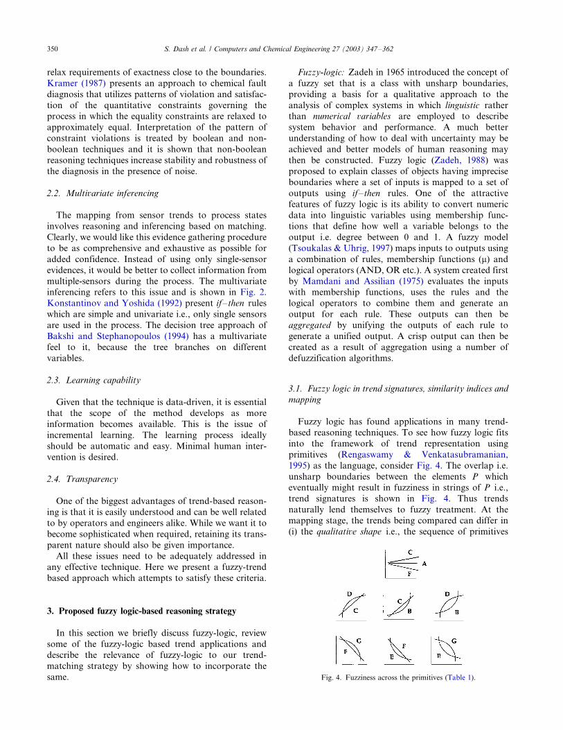
1995) as the language, consider Fig. 4. The overlap i.e.
unsharp boundaries between the elements P which
eventually might result in fuzziness in strings of P i.e.,
trend signatures is shown in Fig. 4. Thus trends
naturally lend themselves to fuzzy treatment. At themapping stage, the trends being compared can differ in
(i) the qualitative shape i.e., the sequence of primitives
Fig. 4. Fuzziness across the primitives (Table 1).
S. Dash et al. / Computers and Chemical Engineering 27 (2003) 347�/362350
Pi , (ii) the duration of Pi and (iii) the magnitude change
accompanying Pi . Fig. 5 shows two visually close trends
which differ in their Pi and their duration. There is a
need to make the technique cognizant of this very realpossibility so that such a scenario can be accommodated
and hence does not affect the performance.
We will be utilizing the trend extraction procedure
based on interval-halving (Dash, Rengaswamy, & Ven-
katasubramanian, 2001) in this work. For each sensor
record [y1, y2,. . ., yn ], at the end of the application of the
technique, we obtain M unimodal regions Ui over [ti ,
ti�1] each (i) described qualitatively by a primitive Pi
and (ii) parameterized quantitatively by a quadratic
qi�Xk�2
k�0
bktk:
Thus the data is transformed into:
Qualitative description: trend Tr�fP1; P2; . . . ; PMg
Quantitative description�fq1; q2; . . . ; qMg (1)
describing it in its entirety. We will make use of both
these descriptions while concentrating more on the
qualitative abstraction. The mapping of trends to states
is achieved in the form of if�/then rules relating the
sensor trends to process state. This is usually a many-to-
one mapping with many sensor trends being mapped to
one fault. For example a rule might read,
If sensor S1 shows trend Tr1 AND sensor S2 shows trend Tr2 . . .
then event is F1
The need here is to develop methods to take care of
imprecision in Tr, as discussed above. In this case the
trends Tr are the qualitative descriptions extracted from
sensor data. Exact matching procedures would necessi-
tate a large number of rules, since we are not flexible in
the comparison procedure. For example, Tr�/BGE,
CF, CGF are all similar to some extent and hence a
strict comparison process will fail to recognize this fact.
A restrictive comparison procedure would require thepresence of all such possibilities in the antecedent of the
rules so that at least one of them matches an observed
trend, which clearly is not practical. Also, an assump-
tion in the trend-analysis scheme is that the sensors
show qualitatively similar trends for the same fault i.e.,
the severity of faults does not distort the trends to a
great extent. This allows us to reason based on patterns,
instead of attaching too much significance to thenumerical values. Of course, this assumption is not
restrictive, since we could always create new categories
of faults if the trends observed are very different at
different severities. Hence we relax the comparison
procedure to define a similarity of match between two
trends. This would make the knowledge-base size
manageable and more insightful. The next section
develops some relaxed criteria to judge the proximityof two trends.
3.1.1. Similarity indices for trend matching
A variety of similarity measures may be defined
depending on the particular application. The set of
primitives (A�/G) are related to each other to some
extent (Fig. 4). As outlined earlier, one of the ways in
which identified trends could differ was in the symbol Pi
i.e., primitive thus contributing to fuzziness. For exam-
ple, B and C are more similar than are B and E. Toquantify this similarity between individual primitives in
a fuzzy manner we define a primitive similarity matrix
shown in Table 1 reflecting this degree of match [0�/1].
Each entry in Table 1, sP1P2, gives a similarity between
P1 and P2. Note that some primitives such as D and G
are treated to be completely different as their funda-
mental behavior is opposite.
The similarity can also be thought of as a syntactic(structural pattern-recognition (Fu, 1982)) approach.
Similar to the template-matching method in decision-
theoretic approach, a similarity or a distance measure
can be defined between a trend representing an un-
known pattern and a string describing a prototype
pattern. Recognition of the unknown pattern can be
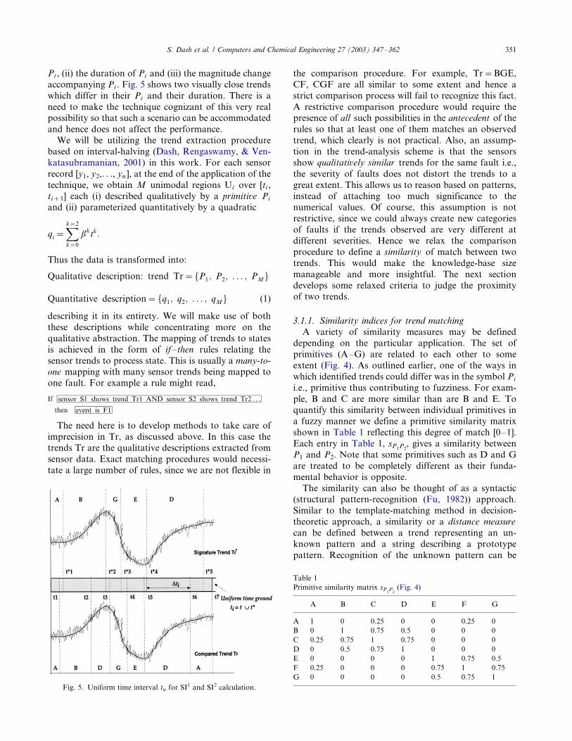
Fig. 5. Uniform time interval tu for SI1 and SI2 calculation.
Table 1
Primitive similarity matrix sP1P2(Fig. 4)
A B C D E F G
A 1 0 0.25 0 0 0.25 0
B 0 1 0.75 0.5 0 0 0
C 0.25 0.75 1 0.75 0 0 0
D 0 0.5 0.75 1 0 0 0
E 0 0 0 0 1 0.75 0.5
F 0.25 0 0 0 0.75 1 0.75
G 0 0 0 0 0.5 0.75 1
S. Dash et al. / Computers and Chemical Engineering 27 (2003) 347�/362 351
carried out on the basis of the maximum-similarity or
minimum-distance criterion. A distance between two
strings x , y can be defined in terms of the minimum
number of error-transformations used to derive onefrom the other. The error transformations are usually
defined in terms of substitution (TS), deletion (TD) and
insertion (TI) errors. These errors are treated as syntax
errors by defining transformations. A weighted Le-
venshtein distance can also be used by defining non-
negative numbers s , g and d to transformations TS, TD
and TI respectively. If x , y are two strings then the
weighted Levenshtein distance is defined as
d(x; y)�minjfskj�gmj�dnjg (2)
where kj , mj and nj are the number of substitution,
deletion and insertion transformations respectively in j .Various other algorithms for string matching can be
found in Cormen, Leiserson, and Rivest (1990).
Here we define two similarity indices, which are
intuitive and simple. Consider a trend in the knowl-
edge-base Tr*�/{P1�, P2�,. . ., PS�} with each Pi� occurringover [ti�, t�i�1] and a trend to be compared Tr�/{P1,
P2,. . ., PM} with each Pi over [ti , ti�1]. In the general
case, both are of different length i.e., M"/S . We definean uniform time ground as the time interval obtained by
the union of both the time stamps tu�/@ /[t , t*]. Let the
number of intervals in tu be R and its length be Tu. This
is shown in Fig. 5 for the two trends. Our similarity
indices are then defined on this tu:
(1) SI1: A simple similarity measure just based on the
sequence can be defined as
SI1�
Xi�R
i�1
sPiPi�
R(3)
This incorporates the similarity of individual patterns,
as given in Table 1. Only the order of the primitives is
considered here.
(2) SI2: The definition of this similarity measure takesinto account the interval-length Dti�/tui�1
�/tui in addi-
tion to the sequence . Thus greater weightage is given to
longer intervals compared to the shorter ones.
SI2�Xi�R
i�1
sPiP+i
DtiTu
(4)
This is more restrictive and calls for a stricter
matching.
We intend to maximize the similarity of the two
trends Tr, Tr* under inspection i.e. desire to evaluate the
trends as closely as possible . This means we would liketo maximize their similarity and so the final similarity
measure we use is the maximum of those defined above.
Thus
SI�max[SI1; SI2] (5)
Once the similarity measure is defined as above, weare in a position to describe the proposed strategy for
fault diagnosis in the next section.
3.2. A two-staged strategy for fault diagnosis
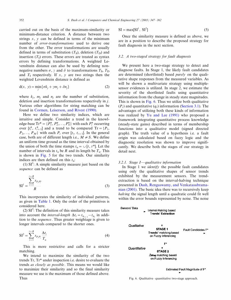
We present here a two-stage strategy to detect and
diagnose faults. In Stage 1, the likely fault candidates
are determined (shortlisted) based purely on the quali-
tative shape responses from the measured variables. As
will be shown a multivariate strategy using multiple-sensor evidences is utilized. In stage 2, we estimate the
severity of the shortlisted faults using quantitative
information from the change in steady state magnitudes.
This is shown in Fig. 6. Thus we utilize both qualitative
(Pi ) and quantitative (qi ) information (Section 3.1). The
advantages of utilizing both these kinds of information
was realized by Yu and Lee (1991) who proposed a
framework integrating quantitative process knowledge(steady-state gains) described in terms of membership
functions into a qualitative model (signed directed
graph). The truth value of a hypothesis i.e. a fault
origin was calculated based on fuzzy logic and the
diagnostic resolution was shown to improve signifi-
cantly. We describe both the stages of our strategy in
detail next.
3.2.1. Stage I*/qualitative information
In Stage 1 we identify the possible fault candidatesusing only the qualitative shapes of sensor trends
exhibited by the measurement sensors. The trend-
extraction is based on the interval-halving technique
presented in Dash, Rengaswamy, and Venkatasubrama-
nian (2001). The basic idea there was to recursively keep
halving the signal length until a quadratic could fit well
within the error bounds represented by noise. The noise
Fig. 6. Qualitative�/quantitative two-stage approach.
S. Dash et al. / Computers and Chemical Engineering 27 (2003) 347�/362352
estimation was done through a wavelet analysis. Details
of the procedure along with extensive examples can be
found in Dash, Rengaswamy, and Venkatasubramanian
(2001).Rule-based knowledge-base: To identify the faults in
this stage we make use of a knowledge-base (Fig. 7)
mapping the fault signatures to the faults in the form of
if�/then rules (Section 3.1). The fault signatures are
patterns that are exhibited by the sensors in response to
a fault, obtained either from dynamic simulations or
historical databases. An example of the i th rule (i th
fault) is shown below
If sensor S1 0 trend Tr+1i AND
sensor S2 0 trend Tr+2i AND . . . then
Fault is Fi
(6)
where i�/1,. . ., M , i.e., there are M such rules relatingsensor trends to the M fault scenarios. Tr1i� refers to the
fault signature exhibited by Sensor S1 for fault Fi . Note
the multivariate nature of the inferencing due to the
conjunction operator AND used here.
Under the assumption that the sensor signatures are
broadly the same under different fault severities, we
require to store only one representative signature for
each sensor for each fault i.e., the antecedents in theknowledge-base in this stage consist of only one fault
signature representative. Thus, if faults are simulated at
severity levels of low, medium and high, the medium
level fault signatures should suffice. As pointed out
earlier, if this is not the case (found by evaluating the
effectiveness) it is always possible to augment the
knowledge-base by creating additional fault classes.
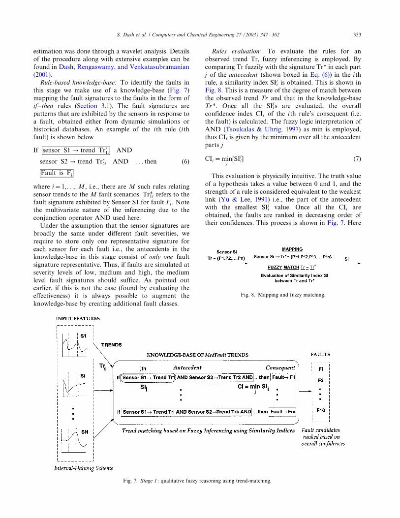
Rules evaluation: To evaluate the rules for an
observed trend Tr, fuzzy inferencing is employed. By
comparing Tr fuzzily with the signature Tr* in each part
j of the antecedent (shown boxed in Eq. (6)) in the i thrule, a similarity index SIi
j is obtained. This is shown in
Fig. 8. This is a measure of the degree of match between
the observed trend Tr and that in the knowledge-base
Tr*. Once all the SIijs are evaluated, the overall
confidence index CIi of the i th rule’s consequent (i.e.
the fault) is calculated. The fuzzy logic interpretation of
AND (Tsoukalas & Uhrig, 1997) as min is employed,
thus CIi is given by the minimum over all the antecedentparts j
CIi�minj[SI
ji] (7)
This evaluation is physically intuitive. The truth value
of a hypothesis takes a value between 0 and 1, and the
strength of a rule is considered equivalent to the weakestlink (Yu & Lee, 1991) i.e., the part of the antecedent
with the smallest SIji value. Once all the CIi are
obtained, the faults are ranked in decreasing order of
their confidences. This process is shown in Fig. 7. Here
Fig. 7. Stage 1 : qualitative fuzzy reasoning using trend-matching.
Fig. 8. Mapping and fuzzy matching.
S. Dash et al. / Computers and Chemical Engineering 27 (2003) 347�/362 353

we try to exploit only the qualitative shape information
and no magnitude information is used. One important
issue here is that of fault resolution . If all the faults can
be qualitatively resolved i.e., distinguishable based onlyon the measured sensor signatures (CIi are well sepa-
rated), then this would result in a high degree of
accuracy in pinpointing the actual fault. However if
this is not the case i.e., the CIi are close, it is necessary to
add more discriminating sensors to resolve the conflict
or look for finer qualitative distinctions for better
discrimination. Of these two options sensor selection
based on fault diagnostic observability criteria usingqualitative models has been researched upon (Raghuraj,
Bhushan, & Rengaswamy, 1999). The second option is
possible in some cases (not always) and one needs to
develop tools that extract features for finer discrimina-
tion automatically. Once the most likely fault candidate
F* is identified, it is passed to the next stage to evaluate
the severity (fault magnitude).
3.2.2. Stage II*/quantitative information
In Stage 1 no quantitative information was used. In
this stage we estimate the magnitude of the detected
fault F* using fuzzy logic. This is shown in Fig. 9. The
knowledge-base in this stage consists of steady-state
magnitude changes DMSilevel in sensor Si accompanying
faults at different levels (low, medium, high). Thisinformation can be obtained from simulations. To
compare the observed magnitude change in sensor Si ,
DMSi with that in the knowledge-base DMS
ilevel, we
adopt a fuzzy-approach instead of strict matching to
lend robustness to the technique. Define the extent of
match at a level as
aSi
level�DMSi
DMSi
level
(8)
with membership function mlevel. Along the same lines as
trend comparison, we also do not desire an exact
magnitude match and hence use a membership function
defined on a normalized magnitude scale a�/[0, 2]
making it level-independent. This is shown in Fig. 10.To be able to do so we define the fault magnitude of F*
as a fuzzy variable with fuzzy values LowF9, Med-
iumF9, HighF9 each having their own membership
functions as shown in Fig. 10. The 9/ signs indicate both
the directions of deviation. All the membership func-
tions used are Gaussian. The knowledge-base (Fig. 9)
consists of rules such as
If sensor aS1level is alevel AND a
S2level is alevel
AND . . . then fault is levelF (9)
Here we make use of the quantitative information inthe trend i.e., magnitude change DM as a result of the
fault. To evaluate the magnitude we again make use of
standard fuzzy reasoning algorithms (Tsoukalas &
Uhrig, 1997) comprising of fuzzification, inferencing
and defuzzification steps (Section 3.1). We use the
Mamdani�/Min implication and centre of area defuzzi-
fication method to estimate the fault as shown in Fig. 9.In the next section, we illustrate the whole methodology
in the fault diagnosis of a reactor. Going back to the
issues discussed in Section 2, we can easily see that the
proposed strategy satisfies all the criteria. It takes care
of the fuzzy aspect in trends allowing inexact matching.
Moreover given the ‘AND’ based inferencing used in the
rules, it is naturally multivariate. The rules are linguistic,
and thus transparent and insightful. Moreover, addingrules to increment or expand the scope of the knowl-
edge-base as processes develop or new events are found
is relatively easy. The knowledge-bases, given their
human-like-reasoning nature, are thus easily related to
and understood, addressing the transparency issue. This
simplicity however does not limit its effectiveness.
4. Illustration
In this section, we show the application of the above
mentioned strategy on an exothermic reactor case study.
4.1. CSTR case study
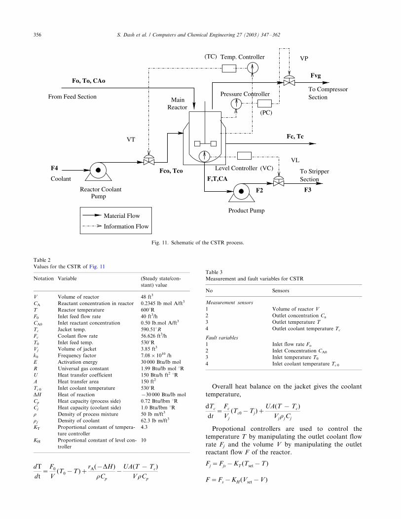
The exothermic CSTR system given by Luyben (1990)is simulated to obtain the manipulated and controlled
variable data to be used by the algorithm. The schematic
of the CSTR system is shown in Fig. 11. The process
involves a liquid phase reaction A(l)0/B(l) This reaction
is highly exothermic and occurs in the reactor. The
temperature controller controls the temperature of the
reactor by manipulating the flow rate of the coolant
flowing through the jacket. The level in the reactor iscontrolled by the level controller by manipulating the
outlet flowrate from the reactor. Both the reactor and
the jacket are modeled with perfectly mixed-tank
dynamics. The reactant volume V and concentration
CA at any time is given by,
dV
dt�F0�F
rA�CAk0e�
E
RT
dCA
dt�
F0
V(CA0
�CA)�rA (10)
Assuming constant heat capacities and densities, an
overall heat balance on the reactor gives the reactant
temperature as,
S. Dash et al. / Computers and Chemical Engineering 27 (2003) 347�/362354
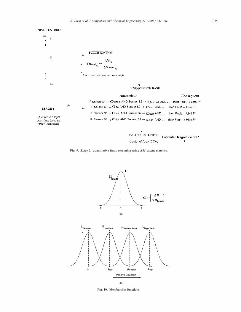
Fig. 10. Membership functions.
Fig. 9. Stage 2: quantitative fuzzy reasoning using DM extent matches.
S. Dash et al. / Computers and Chemical Engineering 27 (2003) 347�/362 355
dT
dt�
F0
V(T0�T)�
rA(�DH)
rCp
�UA(T � Tc)
VrCp
Overall heat balance on the jacket gives the coolant
temperature,
dTc
dt�
Fc
Vj
(Tc0�Tj)�UA(T � Tc)
VjrjCj
Propotional controllers are used to control the
temperature T by manipulating the outlet coolant flow
rate Fj and the volume V by manipulating the outlet
reactant flow F of the reactor.
Fj�Fjs�KT (Tset�T)
F�Fs�KH(Vset�V )
Fig. 11. Schematic of the CSTR process.
Table 2
Values for the CSTR of Fig. 11
Notation Variable (Steady state/con-
stant) value
V Volume of reactor 48 ft3
CA Reactant concentration in reactor 0.2345 lb mol A/ft3
T Reactor temperature 6008RF0 Inlet feed flow rate 40 ft3/h
CA0 Inlet reactant concentration 0.50 lb.mol A/ft3
Tc Jacket temp. 590.518RFc Coolant flow rate 56.626 ft3/h
T0 Inlet feed temp. 5308RVj Volume of jacket 3.85 ft3
k0 Frequency factor 7.08�/1010 /h
E Activation energy 30 000 Btu/lb mol
R Universal gas constant 1.99 Btu/lb mol 8RU Heat transfer coefficient 150 Btu/h ft2 8RA Heat transfer area 150 ft2
Tc 0 Inlet coolant temperature 5308RDH Heat of reaction �/30 000 Btu/lb mol
Cp Heat capacity (process side) 0.72 Btu/lbm 8RCj Heat capacity (coolant side) 1.0 Btu/lbm 8Rr Density of process mixture 50 lb m/ft3
rj Density of coolant 62.3 lb m/ft3
KT Proportional constant of tempera-
ture controller
4.3
KH Proportional constant of level con-
troller
10
Table 3
Measurement and fault variables for CSTR
No Sensors
Measurement sensors
1 Volume of reactor V
2 Outlet concentration Ca
3 Outlet temperature T
4 Outlet coolant temperature Tc
Fault variables
1 Inlet flow rate Fo
2 Inlet Concentration CA0
3 Inlet temperature T0
4 Inlet coolant temperature Tc 0
S. Dash et al. / Computers and Chemical Engineering 27 (2003) 347�/362356
The values of the constants and parameters used in
the simulation and the notation are tabulated in Table 2.
4.2. Knowledge-base and trend fuzziness
To evaluate the proposed strategy fault scenarios are
simulated for knowledge-base construction and testing.The measurement sensors and the fault variables for the
case study are shown in Table 3. The normal behavior of
the process is defined by the steady state, represented by
the primitive ‘A’.
Knowledge-base: To construct the knowledge-base we
carry out fault simulations in positive and negative
deviations for all the 4 input fault variables at a noise
level of 5%. Three levels of step faults (low , medium andhigh ) are simulated in each direction for all the fault
variables (totalling 4�/3�/2�/24 scenarios) as shown in
Table 4. The level of the fault is treated as a fuzzy
variable with fuzzy values low, medium and high. For
Stage 1, which involves only the qualitative shapes of
sensor responses, we only use the shapes from the
medium level faults in the knowledge base. This is to
enforce and evaluate the assumption that the qualitativeshapes are same at different levels of the fault. We thus
retain only one representative (medium) of the fault
scenario. We desire to do with minimal information at
this stage. This amounts to the following 8 scenarios:
F90 , C9
A0, T90 and T9
c0. The fault signatures correspond-
ing to these scenarios form the Stage 1 KB as shown in
Table 5. This knowledge-base is used in fuzzy-inferen-
cing using trend shapes as shown in Fig. 7. Theknowledge-base for Stage 2 on the other hand uses
magnitude information and consists of all the quantita-
tive information for all levels of faults i.e., all 24
scenarios (Section 3.2). The inferencing procedure for
Stage 2 is shown in Fig. 9.
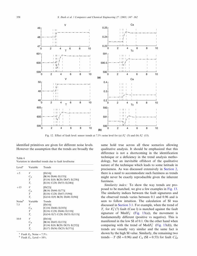
Trend identification and fuzziness: The trends from the
measurement sensors are extracted using the interval-
halving technique described in Dash, Rengaswamy, andVenkatasubramanian (2001). To illustrate the issue of
variability in trend extraction as discussed in Sections 2
and 3.1, we show a sample of the identified trends at
different fault and noise levels. Fig. 12(a and b) shows
the sensor shapes for the F0� fault at levels �/5, �/15
respectively. Although visually the trends look similar,
one can notice slight variations in the extracted trends as
shown in Table 6. Similar behavior can also be seen due
to the effect of noise as shown in Table 6 where the
Table 4
Simulated step fault scenarios
F0 CA0 T0 Tc 0
Level Fault Level Fault Level Fault Level Fault
�/5 LowF0� �/0.05 LowCA0
� �/20 LowT0� �/20 LowTc 0
�
�/10 MedF0� �/0.10 MedCA0
� �/40 MedT0� �/40 MedTc 0
�
�/15 HighF0� �/0.15 HighCA0
� �/60 HighT0� �/60 HighTc 0
�
�/5 LowF0� �/0.05 LowCA0
� �/20 LowT0� �/20 LowTc 0
�
�/10 MedF0� �/0.10 MedCA0
� �/40 MedT0� �/40 MedTc 0
�
�/15 HighF0� �/0.15 HighCA0
� �/60 HighT0� �/60 HighTc 0
�
Table 5
Stage 1 Knowledge base: qualitative shapes of Med faults only
No Fault Variable Fault signatures
1 MedF0� V [D]
CA [C D E]
T [E C D E]
Tc [G E C D E]
2 MedF0� V [F E]
CA [F E]
T [D E]
Tc [C D F E]
3 MedCA0� V [A]
CA [B D F D]
T [B D E]
Tc [B D E]
4 MedCA0� V [A]
CA [E]
T [D D G E]
Tc [G E]
5 MedT0� V [A]
CA [G E D]
T [D D E]
Tc [D G E]
6 MedT0� V [A]
CA [B D]
T [E D]
Tc [D G E D]
7 MedTc0� V [A]
CA [D G E C D F C F A]
T [E B D F E E B D E D]
Tc [C C D F E C G]
8 MedTc0� V [A]
CA [B D]
T [E D]
Tc [F]
S. Dash et al. / Computers and Chemical Engineering 27 (2003) 347�/362 357
identified primitives are given for different noise levels.
However the assumption that the trends are broadly the
same hold true across all these scenarios allowing
qualitative analysis. It should be emphasized that this
difference is not a shortcoming in the identification
technique or a deficiency in the trend analysis metho-
dology, but an inevitable offshoot of the qualitative
nature of the technique which leads to some latitude in
preciseness. As was discussed extensively in Section 2,
there is a need to accommodate such fuzziness as trends
might never be exactly reproducible given the inherent
fuzziness.Similarity index: To show the way trends are pro-
posed to be matched, we give a few examples in Fig. 13.
The similarity indices between the fault signatures and
the observed trends varies between 0.1 and 0.96 and is
seen to follow intuition. The calculation of SI was
discussed in Section 3.1. For example, when the trend of
Tc for F�0 (7) fault (Case l) is matched against the fault
signature of MedF�0 (Fig. 13(a)), the movement is
fundamentally different (positive vs negative). This is
manifested in the low SI of 0.1. On the other hand when
comparing with the trend of MedF0� (Fig. 13(d)), the
trends are visually very similar and the same fact is
shown by the high SI value. Similarly, the remaining two
trends*/T (SI�/0.96) and CA (SI�/0.53) for fault C�A0
Fig. 12. Effect of fault level: sensor trends at 7.5% noise level for (a) F0� (5) and (b) F0
� (15).
Table 6
Variation in identified trends due to fault level/noise
Levela Variable Trends
�/5 V [D(14)]
CA [B(14) D(46) E(135)]
T [F(14) E(8) B(28) D(47) E(238)]
Tc [E(16) C(28) D(53) E(246)]
�/15 V [D(22)]
CA [B(14) D(44) E(77)]
T [E(16) C(28) D(47) F(94)]
Tc [G(14) E(9) B(28) D(48) E(94)]
Noiseb Variable Trends
7.5 V [D(14)]
CA [C(14) D(46) E(103)]
T [E(16) C(28) D(46) E(118)]
Tc [G(14) E(7) C(28) D(53) E(115)]
10.0 V [D(14)]
CA [B(14) D(45) E(133)]
T [F(14) E(8) B(28) D(53) E(232)]
Tc [E(17) D(56) D(25) E(371)]
a Fault F0, Noise�/7.5%.b Fault F0 , Level�/10%.
S. Dash et al. / Computers and Chemical Engineering 27 (2003) 347�/362358
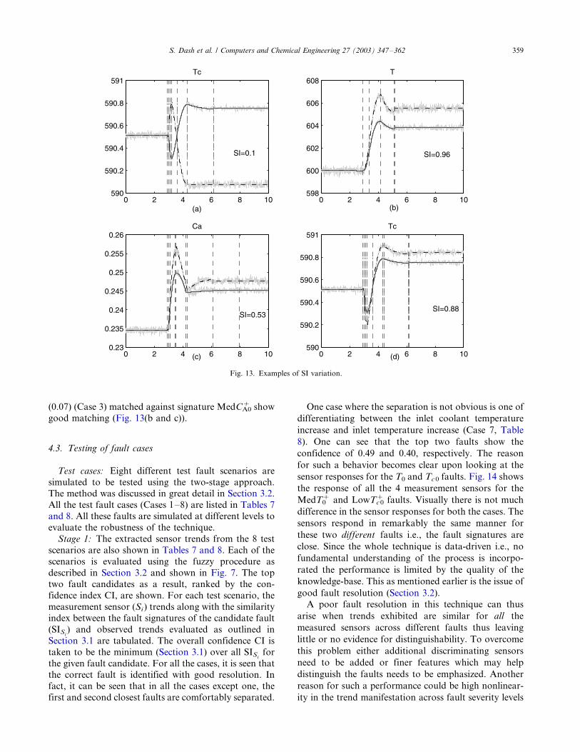
(0.07) (Case 3) matched against signature MedC�A0 show
good matching (Fig. 13(b and c)).
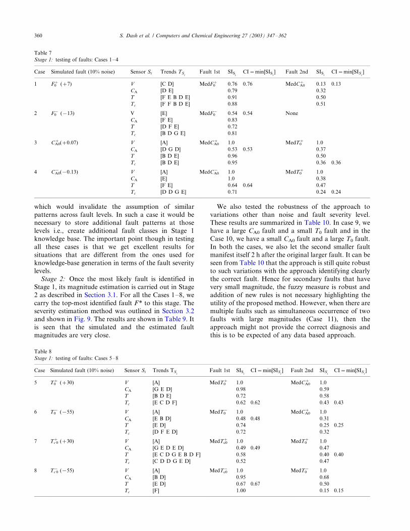
4.3. Testing of fault cases
Test cases: Eight different test fault scenarios are
simulated to be tested using the two-stage approach.The method was discussed in great detail in Section 3.2.
All the test fault cases (Cases 1�/8) are listed in Tables 7
and 8. All these faults are simulated at different levels to
evaluate the robustness of the technique.
Stage 1: The extracted sensor trends from the 8 test
scenarios are also shown in Tables 7 and 8. Each of the
scenarios is evaluated using the fuzzy procedure as
described in Section 3.2 and shown in Fig. 7. The toptwo fault candidates as a result, ranked by the con-
fidence index CI, are shown. For each test scenario, the
measurement sensor (Si) trends along with the similarity
index between the fault signatures of the candidate fault
(SISi) and observed trends evaluated as outlined in
Section 3.1 are tabulated. The overall confidence CI is
taken to be the minimum (Section 3.1) over all SISifor
the given fault candidate. For all the cases, it is seen thatthe correct fault is identified with good resolution. In
fact, it can be seen that in all the cases except one, the
first and second closest faults are comfortably separated.
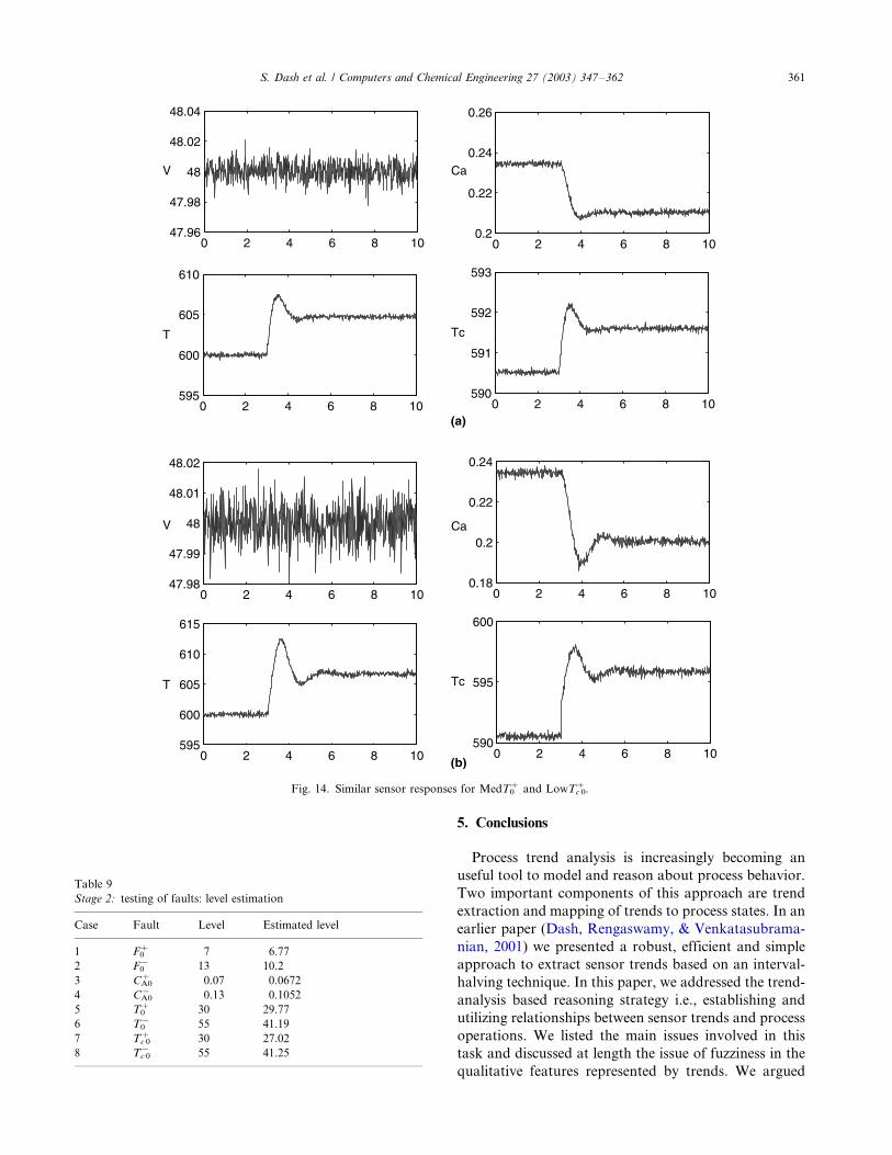
One case where the separation is not obvious is one of
differentiating between the inlet coolant temperature
increase and inlet temperature increase (Case 7, Table
8). One can see that the top two faults show the
confidence of 0.49 and 0.40, respectively. The reason
for such a behavior becomes clear upon looking at the
sensor responses for the T0 and Tc0 faults. Fig. 14 shows
the response of all the 4 measurement sensors for the
MedT�0 and LowT�
c0 faults. Visually there is not much
difference in the sensor responses for both the cases. The
sensors respond in remarkably the same manner for
these two different faults i.e., the fault signatures are
close. Since the whole technique is data-driven i.e., no
fundamental understanding of the process is incorpo-
rated the performance is limited by the quality of the
knowledge-base. This as mentioned earlier is the issue of
good fault resolution (Section 3.2).
A poor fault resolution in this technique can thus
arise when trends exhibited are similar for all the
measured sensors across different faults thus leaving
little or no evidence for distinguishability. To overcome
this problem either additional discriminating sensors
need to be added or finer features which may help
distinguish the faults needs to be emphasized. Another
reason for such a performance could be high nonlinear-
ity in the trend manifestation across fault severity levels
Fig. 13. Examples of SI variation.
S. Dash et al. / Computers and Chemical Engineering 27 (2003) 347�/362 359
which would invalidate the assumption of similar
patterns across fault levels. In such a case it would be
necessary to store additional fault patterns at those
levels i.e., create additional fault classes in Stage 1
knowledge base. The important point though in testing
all these cases is that we get excellent results for
situations that are different from the ones used for
knowledge-base generation in terms of the fault severity
levels.
Stage 2: Once the most likely fault is identified in
Stage 1, its magnitude estimation is carried out in Stage
2 as described in Section 3.1. For all the Cases 1�/8, we
carry the top-most identified fault F* to this stage. The
severity estimation method was outlined in Section 3.2
and shown in Fig. 9. The results are shown in Table 9. It
is seen that the simulated and the estimated fault
magnitudes are very close.
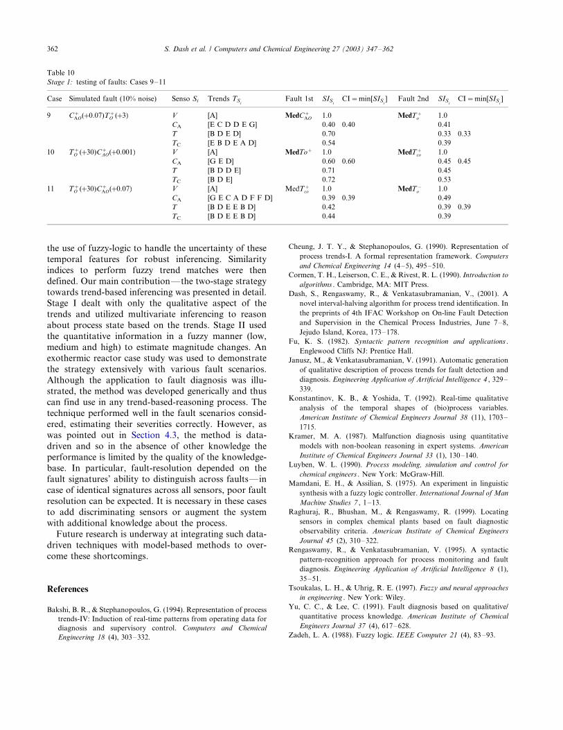
We also tested the robustness of the approach to
variations other than noise and fault severity level.
These results are summarized in Table 10. In case 9, we
have a large CA0 fault and a small T0 fault and in the
Case 10, we have a small CA0 fault and a large T0 fault.
In both the cases, we also let the second smaller fault
manifest itself 2 h after the original larger fault. It can be
seen from Table 10 that the approach is still quite robust
to such variations with the approach identifying clearly
the correct fault. Hence for secondary faults that have
very small magnitude, the fuzzy measure is robust and
addition of new rules is not necessary highlighting the
utility of the proposed method. However, when there are
multiple faults such as simultaneous occurrence of two
faults with large magnitudes (Case 11), then the
approach might not provide the correct diagnosis and
this is to be expected of any data based approach.
Table 8
Stage 1: testing of faults: Cases 5�/8
Case Simulated fault (10% noise) Sensor Si Trends TSi
Fault 1st SISi
CI�/min[SISi] Fault 2nd SIS
iCI�/min[SIS
i]
5 T0� (�/30) V [A] MedT0
� 1.0 MedCA0� 1.0
CA [G E D] 0.98 0.59
T [B D E] 0.72 0.58
Tc [E C D F] 0.62 0.62 0.43 0.43
6 T0� (�/55) V [A] MedT0
� 1.0 MedCA0� 1.0
CA [E B D] 0.48 0.48 0.31
T [E D] 0.74 0.25 0.25
Tc [D F E D] 0.72 0.32
7 Tc 0� (�/30) V [A] MedTc0
� 1.0 MedT0� 1.0
CA [G E D E D] 0.49 0.49 0.47
T [E C D G E B D F] 0.58 0.40 0.40
Tc [C D D G E D] 0.52 0.47
8 Tc 0� (�/55) V [A] MedTc0
� 1.0 MedT0� 1.0
CA [B D] 0.95 0.68
T [E D] 0.67 0.67 0.50
Tc [F] 1.00 0.15 0.15
Table 7
Stage 1: testing of faults: Cases 1�/4
Case Simulated fault (10% noise) Sensor Si Trends TSi
Fault 1st SISi
CI�/min[SISi] Fault 2nd SIS
iCI�/min[SIS
i]
1 F0� (�/7) V [C D] MedF0
� 0.76 0.76 MedCA0� 0.13 0.13
CA [D E] 0.79 0.32
T [F E B D E] 0.91 0.50
Tc [F F B D E] 0.88 0.51
2 F0� (�/13) V [E] MedF0
� 0.54 0.54 None
CA [F E] 0.83
T [D F E] 0.72
Tc [B D G E] 0.81
3 CA0� (�/0.07) V [A] MedCA0
� 1.0 MedT0� 1.0
CA [D G D] 0.53 0.53 0.37
T [B D E] 0.96 0.50
Tc [B D E] 0.95 0.36 0.36
4 CA0� (�/0.13) V [A] MedCA0
� 1.0 MedT0� 1.0
CA [E] 1.0 0.38
T [F E] 0.64 0.64 0.47
Tc [D D G E] 0.71 0.24 0.24
S. Dash et al. / Computers and Chemical Engineering 27 (2003) 347�/362360
5. Conclusions
Process trend analysis is increasingly becoming an
useful tool to model and reason about process behavior.
Two important components of this approach are trend
extraction and mapping of trends to process states. In an
earlier paper (Dash, Rengaswamy, & Venkatasubrama-
nian, 2001) we presented a robust, efficient and simple
approach to extract sensor trends based on an interval-
halving technique. In this paper, we addressed the trend-
analysis based reasoning strategy i.e., establishing and
utilizing relationships between sensor trends and process
operations. We listed the main issues involved in this
task and discussed at length the issue of fuzziness in the
qualitative features represented by trends. We argued
Fig. 14. Similar sensor responses for MedT0� and LowTc 0
�.
Table 9
Stage 2: testing of faults: level estimation
Case Fault Level Estimated level
1 F0� 7 6.77
2 F0� 13 10.2
3 CA0� 0.07 0.0672
4 CA0� 0.13 0.1052
5 T0� 30 29.77
6 T0� 55 41.19
7 Tc 0� 30 27.02
8 Tc 0� 55 41.25
S. Dash et al. / Computers and Chemical Engineering 27 (2003) 347�/362 361
the use of fuzzy-logic to handle the uncertainty of these
temporal features for robust inferencing. Similarity
indices to perform fuzzy trend matches were then
defined. Our main contribution*/the two-stage strategy
towards trend-based inferencing was presented in detail.Stage I dealt with only the qualitative aspect of the
trends and utilized multivariate inferencing to reason
about process state based on the trends. Stage II used
the quantitative information in a fuzzy manner (low,
medium and high) to estimate magnitude changes. An
exothermic reactor case study was used to demonstrate
the strategy extensively with various fault scenarios.
Although the application to fault diagnosis was illu-strated, the method was developed generically and thus
can find use in any trend-based-reasoning process. The
technique performed well in the fault scenarios consid-
ered, estimating their severities correctly. However, as
was pointed out in Section 4.3, the method is data-
driven and so in the absence of other knowledge the
performance is limited by the quality of the knowledge-
base. In particular, fault-resolution depended on thefault signatures’ ability to distinguish across faults*/in
case of identical signatures across all sensors, poor fault
resolution can be expected. It is necessary in these cases
to add discriminating sensors or augment the system
with additional knowledge about the process.
Future research is underway at integrating such data-
driven techniques with model-based methods to over-
come these shortcomings.
References
Bakshi, B. R., & Stephanopoulos, G. (1994). Representation of process
trends-IV: Induction of real-time patterns from operating data for
diagnosis and supervisory control. Computers and Chemical
Engineering 18 (4), 303�/332.
Cheung, J. T. Y., & Stephanopoulos, G. (1990). Representation of
process trends-I. A formal representation framework. Computers
and Chemical Engineering 14 (4�/5), 495�/510.Cormen, T. H., Leiserson, C. E., & Rivest, R. L. (1990). Introduction to
algorithms . Cambridge, MA: MIT Press.
Dash, S., Rengaswamy, R., & Venkatasubramanian, V., (2001). A
novel interval-halving algorithm for process trend identification. In
the preprints of 4th IFAC Workshop on On-line Fault Detection
and Supervision in the Chemical Process Industries, June 7�/8,Jejudo Island, Korea, 173�/178.
Fu, K. S. (1982). Syntactic pattern recognition and applications .
Englewood Cliffs NJ: Prentice Hall.
Janusz, M., & Venkatasubramanian, V. (1991). Automatic generation
of qualitative description of process trends for fault detection and
diagnosis. Engineering Application of Artificial Intelligence 4 , 329�/339.
Konstantinov, K. B., & Yoshida, T. (1992). Real-time qualitative
analysis of the temporal shapes of (bio)process variables.
American Institute of Chemical Engineers Journal 38 (11), 1703�/1715.
Kramer, M. A. (1987). Malfunction diagnosis using quantitative
models with non-boolean reasoning in expert systems. American
Institute of Chemical Engineers Journal 33 (1), 130�/140.Luyben, W. L. (1990). Process modeling, simulation and control for
chemical engineers . New York: McGraw-Hill.
Mamdani, E. H., & Assilian, S. (1975). An experiment in linguistic
synthesis with a fuzzy logic controller. International Journal of Man
Machine Studies 7 , 1�/13.Raghuraj, R., Bhushan, M., & Rengaswamy, R. (1999). Locating
sensors in complex chemical plants based on fault diagnostic
observability criteria. American Institute of Chemical Engineers
Journal 45 (2), 310�/322.Rengaswamy, R., & Venkatasubramanian, V. (1995). A syntactic
pattern-recognition approach for process monitoring and fault
diagnosis. Engineering Application of Artificial Intelligence 8 (1),
35�/51.Tsoukalas, L. H., & Uhrig, R. E. (1997). Fuzzy and neural approaches
in engineering . New York: Wiley.
Yu, C. C., & Lee, C. (1991). Fault diagnosis based on qualitative/
quantitative process knowledge. American Institute of Chemical
Engineers Journal 37 (4), 617�/628.Zadeh, L. A. (1988). Fuzzy logic. IEEE Computer 21 (4), 83�/93.
Table 10
Stage 1: testing of faults: Cases 9�/11
Case Simulated fault (10% noise) Senso Si Trends TSi
Fault 1st SISi
CI�/min[SISi] Fault 2nd SIS
iCI�/min[SIS
i]
9 /C�AO(�0:07)T�
O (�3)/ V [A] Med/C�AO/ 1.0 Med/T�
o / 1.0
CA [E C D D E G] 0.40 0.40 0.41
T [B D E D] 0.70 0.33 0.33
TC [E B D E A D] 0.54 0.39
10 /T�O (�30)C�
AO(�0:001)/ V [A] Med/To�/ 1.0 Med/T�co/ 1.0
CA [G E D] 0.60 0.60 0.45 0.45
T [B D D E] 0.71 0.45
TC [B D E] 0.72 0.53
11 /T�O (�30)C�
AO(�0:07)/ V [A] Med/T�co/ 1.0 Med/T�
o / 1.0
CA [G E C A D F F D] 0.39 0.39 0.49
T [B D E E B D] 0.42 0.39 0.39
TC [B D E E B D] 0.44 0.39
S. Dash et al. / Computers and Chemical Engineering 27 (2003) 347�/362362