Futures Prices in a Production Economy withInvestment Constraints∗

Leonid Kogan†, Dmitry Livdan‡, and Amir Yaron§

This Draft: March 29, 2005

Abstract

We document a new stylized fact regarding the term-structure of futures volatility.We show that the relationship between the volatility of futures prices and the slopeof the term structure of prices is non-monotone and has a “V-shape”. This aspect ofthe data cannot be generated by basic models that emphasize storage while this factis consistent with models that emphasize investment constraints or, more generally,time-varying supply-elasticity. We develop an equilibrium model in which futuresprices are determined endogenously in a production economy in which investmentis both irreversible and is capacity constrained. Investment constraints affect firmsinvestment decisions, which in turn determine the dynamic properties of their outputand consequently imply that the supply-elasticity of the commodity changes over time.Since demand shocks must be absorbed either by changes in prices, or by changes insupply, time-varying supply-elasticity results in time-varying volatility of futures prices.Calibrating this model, we show it is quantitatively consistent with the aforementioned“V-shape” relationship between the volatility of futures prices and the slope of theterm-structure.

∗We are grateful to Kerry Back, Pierre Collin-Dufresne, Francis Longstaff and Craig Pirrong, as well asseminar participants at Northwestern University, Texas A&M University, 2004 Western Finance Associationmeeting, 2004 Society of Economic Dynamics meeting, and 2004 European Econometric Society meeting foruseful suggestions. We also thank Krishna Ramaswamy for providing us with the futures data. Financialsupport from the Rodney L. White Center for Financial Research at the Wharton school is gratefullyacknowledged.

†Sloan School of Management, Massachusetts Institute of Technology and NBER. Cambridge, MA 02142.Phone: (617) 253-2289. Fax: (617) 258-6855. E-mail: lkogan@mit.edu.

‡Bauer School of Business, University of Houston. Houston, TX 77204, Phone:(713) 743-4813. Fax: (713)743-4755. Email: dlivdan@uh.edu.

§The Wharton School, University of Pennsylvania and NBER. Philadelphia, PA 19104. Phone: (215)-898-1241. Fax: (215) 898-6200. E-mail: yaron@wharton.upenn.edu.

1 Introduction

In recent years commodity markets have experienced dramatic growth in trading volume,

the variety of contracts, and the range of underlying commodities. There also has been

a great demand for derivative instruments utilizing operational contingencies embedded in

delivery contracts. For all these reasons there is a widespread interest in models for pricing

and hedging commodity-linked contingent claims. Besides practical interest, commodities

offer a rich variety of empirical properties, which make them strikingly different from stocks,

bonds and other conventional financial assets. Notable properties of futures include, among

others: (i) Commodity futures prices are often ”backwardated” in that they decline with

time-to-delivery, (ii) Spot and futures prices are mean reverting for many commodities,

(iii) Commodity prices are strongly heteroscedastic and price volatility is correlated with

the degree of backwardation, and (iv) Unlike financial assets, many commodities have

pronounced seasonalities in both price levels and volatilities.

The ‘theory of storage’ of Kaldor (1939), Working (1948, 1949) and Telser (1958) has

been the foundation of the theoretical explorations of futures/forward prices and convenience

yields (value of the immediate ownership of the physical commodity). Based on this

theory researchers have adopted two approaches to modelling commodity prices. The first

approach is mainly statistical in nature and requires an exogenous specification of the

‘convenience yield’ process for a commodity (e.g., Brennan and Schwartz (1985), Brennan

(1991), and Schwartz (1997)). The second strand of the literature derives the price processes

endogenously in an equilibrium valuation framework with competitive storage (e.g., Williams

and Wright (1991), Deaton and Laroque (1992, 1996), Routledge, Seppi, and Spatt (2000)).

The appealing aspect of this approach is its ability to link the futures prices to the level of

inventories and hence derive additional testable restrictions on the price processes.

From a theoretical perspective the models based on competitive storage ignore the

production side of the economy, and consequently they suffer from an important limitation.

Inventory dynamics have little if any impact on the long-run properties of commodity prices,

which in such models are driven mostly by the exogenously specified demand process. In

particular, prices in such models tend to mean revert too fast relative to what is observed

1

in the data (see Routledge et. al. (2000)), and more importantly the model can not address

the rich term-structure dynamics of return volatility.

In this paper we document an important new stylized fact regarding the property of the

term structure of volatility of futures prices. We demonstrate that the relationship between

the volatility of futures prices and the slope of the forward curve (the basis) is non-monotone

and has a “V-shape”. Specifically, conditionally on a negatively sloped term structure, the

relation between the volatility of futures prices and the slope of the forward curve is negative.

On the other hand, conditionally on a positively sloped term structure, the relation between

the volatility and the basis is positive. This aspect of the data cannot be generated by basic

models that emphasize storage, since such models imply a monotone relation between futures

price volatility and the slope of the forward curve (see Routledge et. al. (2000)).

In light of the aforementioned stylized fact, we explore an alternative model characterizing

the mechanism of futures price formation. Future prices are determined endogenously in an

equilibrium production economy featuring constraints on investment, such as irreversibility.

Investment constraints affect firms investment decisions, which in turn determine the

dynamic properties of their output. In particular, because of the binding constraints on

investment, supply-elasticity of the commodity changes over time. Since demand shocks

must be absorbed either by changes in prices, or by changes in supply, time-varying supply-

elasticity results in time-varying volatility of futures prices. In our calibration below we show

that the model can also generate these patterns in a manner that is quantitatively similar

to the data.

There exists very little theoretical work investigating the pricing of futures on

commodities using production economy framework. Casassus, Collin-Dufresne and

Routledge (2004) also analyze a model of equilibrium spot and futures oil prices in a general

equilibrium production economy but with two goods. In their model production of the

consumption good requires two inputs: the consumption good and oil. Oil is produced

by wells whose flow rate is costly to adjust. Unlike our paper, however, their focus is on

providing an appropriate specification for the joint dynamics of spot price, convenience yield

and interest rates. Moreover, their model features only one constraint (irreversibility of

investment) required for generating the stylized fact that we document here.

2

The rest of the paper is organized as follows. In Section 2 we describe our data analysis

regarding future prices. Section 3 develops the model’s economy as well as presents the spot

price and prices of financial assets derived in competitive equilibrium setting. In Section 4,

we study quantitative implications of the model. Section 5 provides conclusions.

2 Empirical Analysis

We concentrate our empirical study on three commodities: crude oil, heating oil, and

unleaded gasoline. Our data consists of daily futures prices for three contracts: NYMEX

heating oil contract (HO) for the period from 1979 to 2000, NYMEX light sweet crude oil

contract (CL) for the period from 1982 to 2000, and NYMEX unleaded New York harbor

gasoline futures (HU) for the period from 1985 to 2000. Following previous work by Routledge

et. al (2000), the data is sorted by contract horizon with the ‘one-month’ contract being

the contract with the earliest delivery date, the ‘two-month’ contract having next earliest

delivery date, etc.1. We consider contracts with up to 12 months to delivery when contract

‘matures’ since liquidity and data availability is good for these horizons for all three contracts

used in this study.2 Since we are using daily data, our dataset is sufficiently large: it ranges

from 2500 to 3500 data points across different contracts and maturities.

Instead of directly using futures prices, P (t, T ), we use daily percent changes, R(t, T ) =

P (t,T )P (t−1,T )

. Percent price changes are not susceptible as much as price levels to seasonalities and

trends, and therefore their volatility is more suitable for empirical analysis. We then proceed

by constructing the term structure of the unconditional and conditional volatilities of daily

percent changes on futures for all three contracts. In calculating conditional moments we

classify the futures curve at each date t as to whether one trading day earlier the curve

was in backwardation or contango (based on the shortest and third shortest maturity prices

1In our data set, for each of the commodities, on any given calendar day there are several contractsavailable with different time to delivery measured in days. The difference in delivery times between thesecontracts is at least 32 days or more. We utilize the following procedure for converting delivery times tothe monthly scale. For each contract we divide the number of days it has left to maturity by 30 (theaverage number of days in a month), and then round off the resultant. For days when contract with time todelivery of less than 15 days is traded, we add one “month” to the contract horizon obtained using the aboveprocedure for all contracts traded on such days. The data is then sorted into bins based on the contracthorizon measured in months.

2We refer to this time to delivery as time to maturity throughout the paper.

3

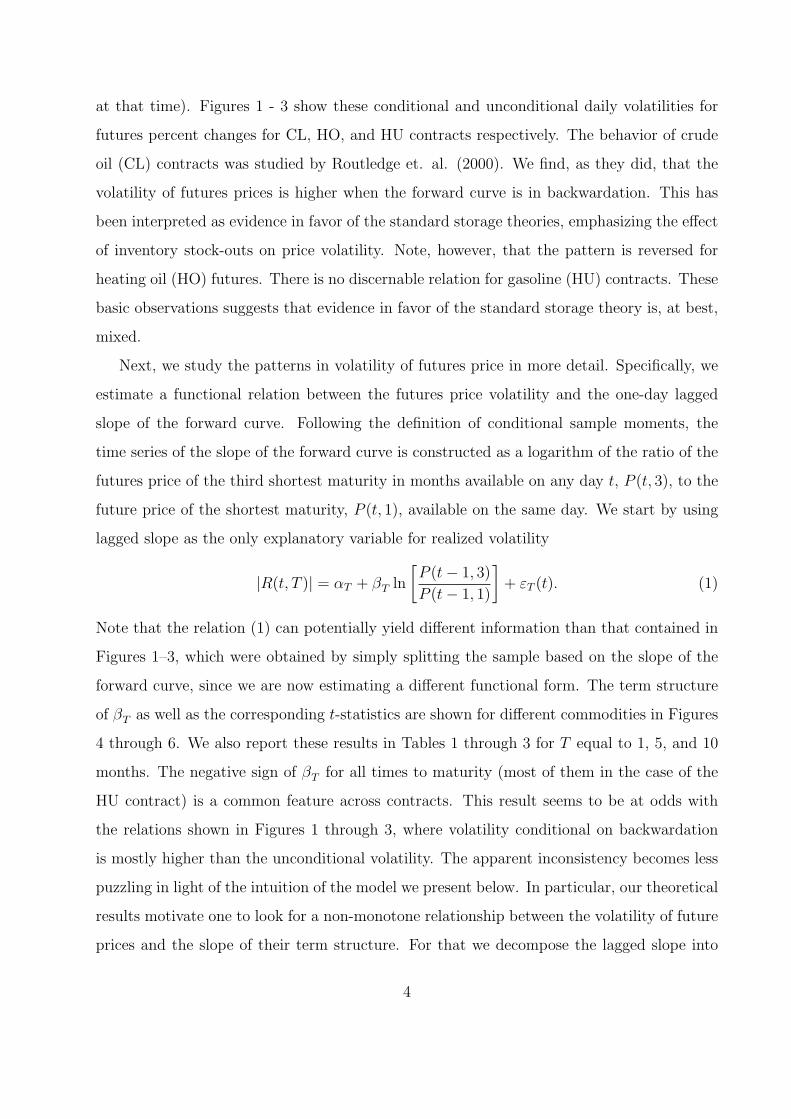
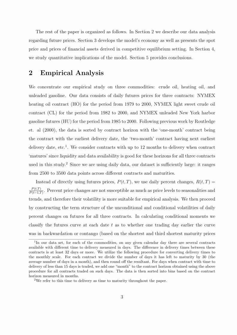
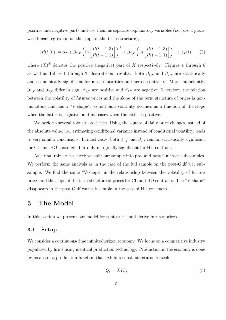
at that time). Figures 1 - 3 show these conditional and unconditional daily volatilities for

futures percent changes for CL, HO, and HU contracts respectively. The behavior of crude

oil (CL) contracts was studied by Routledge et. al. (2000). We find, as they did, that the

volatility of futures prices is higher when the forward curve is in backwardation. This has

been interpreted as evidence in favor of the standard storage theories, emphasizing the effect

of inventory stock-outs on price volatility. Note, however, that the pattern is reversed for

heating oil (HO) futures. There is no discernable relation for gasoline (HU) contracts. These

basic observations suggests that evidence in favor of the standard storage theory is, at best,

mixed.

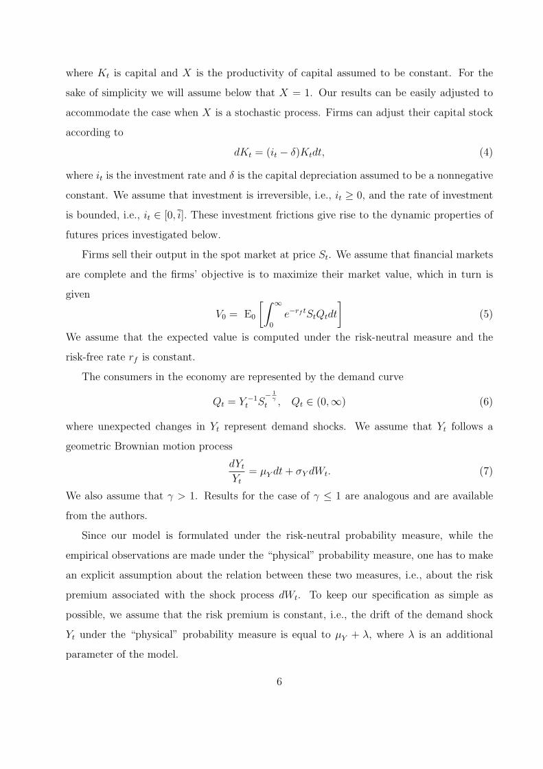
Next, we study the patterns in volatility of futures price in more detail. Specifically, we

estimate a functional relation between the futures price volatility and the one-day lagged

slope of the forward curve. Following the definition of conditional sample moments, the

time series of the slope of the forward curve is constructed as a logarithm of the ratio of the

futures price of the third shortest maturity in months available on any day t, P (t, 3), to the

future price of the shortest maturity, P (t, 1), available on the same day. We start by using

lagged slope as the only explanatory variable for realized volatility

|R(t, T )| = αT + βT ln

[P (t− 1, 3)

P (t− 1, 1)

]+ εT (t). (1)

Note that the relation (1) can potentially yield different information than that contained in

Figures 1–3, which were obtained by simply splitting the sample based on the slope of the

forward curve, since we are now estimating a different functional form. The term structure

of βT as well as the corresponding t-statistics are shown for different commodities in Figures

4 through 6. We also report these results in Tables 1 through 3 for T equal to 1, 5, and 10

months. The negative sign of βT for all times to maturity (most of them in the case of the

HU contract) is a common feature across contracts. This result seems to be at odds with

the relations shown in Figures 1 through 3, where volatility conditional on backwardation

is mostly higher than the unconditional volatility. The apparent inconsistency becomes less

puzzling in light of the intuition of the model we present below. In particular, our theoretical

results motivate one to look for a non-monotone relationship between the volatility of future

prices and the slope of their term structure. For that we decompose the lagged slope into

4

positive and negative parts and use them as separate explanatory variables (i.e., use a piece-

wise linear regression on the slope of the term structure),

|R(t, T )| = αT + β1,T

(ln

[P (t− 1, 3)

P (t− 1, 1)

])+

+ β2,T

(ln

[P (t− 1, 3)

P (t− 1, 1)

])−+ εT (t), (2)

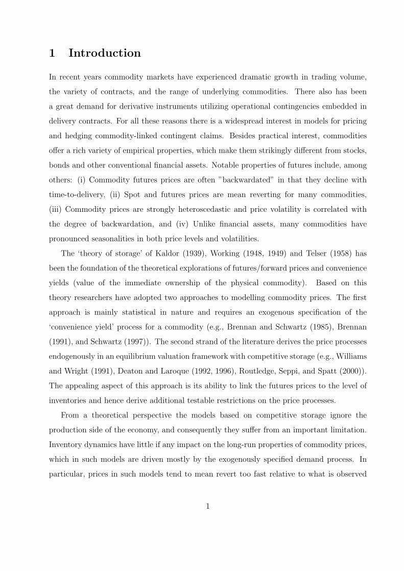
where (X)± denotes the positive (negative) part of X respectively. Figures 4 through 6

as well as Tables 1 through 3 illustrate our results. Both β1,T and β2,T are statistically

and economically significant for most maturities and across contracts. More importantly,

β1,T and β2,T differ in sign: β1,T are positive and β2,T are negative. Therefore, the relation

between the volatility of futures prices and the slope of the term structure of prices is non-

monotone and has a “V-shape”: conditional volatility declines as a function of the slope

when the latter is negative, and increases when the latter is positive.

We perform several robustness checks. Using the square of daily price changes instead of

the absolute value, i.e., estimating conditional variance instead of conditional volatility, leads

to very similar conclusions. In most cases, both β1,T and β2,T remain statistically significant

for CL and HO contracts, but only marginally significant for HU contract.

As a final robustness check we split our sample into pre- and post-Gulf war sub-samples.

We perform the same analysis as in the case of the full sample on the post-Gulf war sub-

sample. We find the same “V-shape” in the relationship between the volatility of futures

prices and the slope of the term structure of prices for CL and HO contracts. The “V-shape”

disappears in the post-Gulf war sub-sample in the case of HU contracts.

3 The Model

In this section we present our model for spot prices and derive futures prices.

3.1 Setup

We consider a continuous-time infinite-horizon economy. We focus on a competitive industry

populated by firms using identical production technology. Production in the economy is done

by means of a production function that exhibits constant returns to scale

Qt = XKt, (3)

5

where Kt is capital and X is the productivity of capital assumed to be constant. For the

sake of simplicity we will assume below that X = 1. Our results can be easily adjusted to

accommodate the case when X is a stochastic process. Firms can adjust their capital stock

according to

dKt = (it − δ)Ktdt, (4)

where it is the investment rate and δ is the capital depreciation assumed to be a nonnegative

constant. We assume that investment is irreversible, i.e., it ≥ 0, and the rate of investment

is bounded, i.e., it ∈ [0, i]. These investment frictions give rise to the dynamic properties of

futures prices investigated below.

Firms sell their output in the spot market at price St. We assume that financial markets

are complete and the firms’ objective is to maximize their market value, which in turn is

given

V0 = E0

[∫ ∞

0

e−rf tStQtdt

](5)

We assume that the expected value is computed under the risk-neutral measure and the

risk-free rate rf is constant.

The consumers in the economy are represented by the demand curve

Qt = Y −1t S

− 1γ

t , Qt ∈ (0,∞) (6)

where unexpected changes in Yt represent demand shocks. We assume that Yt follows a

geometric Brownian motion process

dYt

Yt

= µY dt + σY dWt. (7)

We also assume that γ > 1. Results for the case of γ ≤ 1 are analogous and are available

from the authors.

Since our model is formulated under the risk-neutral probability measure, while the

empirical observations are made under the “physical” probability measure, one has to make

an explicit assumption about the relation between these two measures, i.e., about the risk

premium associated with the shock process dWt. To keep our specification as simple as

possible, we assume that the risk premium is constant, i.e., the drift of the demand shock

Yt under the “physical” probability measure is equal to µY + λ, where λ is an additional

parameter of the model.

6

3.2 Equilibrium Investment and Prices

Following Lucas and Prescott (1971), we characterize the equilibrium investment policy as

a solution of the social planner’s problem. Specifically, we define the surplus function3

U(Yt, Qt) =

∫ Qt

1

St (q) dq = Y −γt

∫ Qt

1

Q−γ dQ = Y −γt

Q1−γt − 1

1− γ. (8)

The social planner maximizes total surplus net of investment costs

maxit∈[0,i]

E0

[∫ ∞

0

e−rf t

(Y −γ

t

K1−γt

1− γ− itKt

)dt

](9)

subject to the dynamics of the demand curve and the capital accumulation rule

dKt = (it − δ)Ktdt,

dYt

Yt

= µY dt + σY dWt,

Kt ≥ 0, , ∀t ≥ 0.

The details of the solution are given in the Appendix. The equilibrium investment policy

is given by

i∗t =

{i, ωt ≤ ω∗

0, ωt > ω∗

where ωt = ln(KtYt) and ω∗ is given in the Appendix. The evolution of the state variable ωt

under the risk-neutral measure is governed by

dωt =

[−δ + i∗t + µY −

1

2σ2

Y

]dt + σY dWt. (10)

Therefore, as long as 0 < δ − µY + 12σ2

Y < i, ωt has a stationary long-run distribution

p(ω) =2µ+µ−

iσ2Y

e− 2µ+

σ2Y

(ω∗−ω)ω ≤ ω∗

e− 2µ−

σ2Y

(ω−ω∗)ω > ω∗

. (11)

where we define the two constants µ− = δ − µY + 12σ2

Y and µ+ = i− µ−. The condition for

stationarity of ωt can be re-stated as 0 < µ− < i. The details of the derivation are provided

3Starting the integration at 1 is inconsequential for our analysis. Recall that Q is restricted to be strictlypositive guaranteeing a well defined objective function in equation (9). Starting the integration at anypositive point below one would only add a constant to the objective function in equation (9) not affectingthe first order conditions.

7

in the Appendix. The spot price process of firms’ output is related to the equilibrium capital

stock by the inverse demand curve

St = [KtYt]−γ = e−γωt , (12)

It is worth mapping our general investment constraint model to the oil industry. Oil (Q)

is the output produced using physical capital K (e.g., refineries, pipes). Implicitly we are

assuming there is an infinite supply of underground oil, and production is constrained by the

existing capital stock K. This supply of capital and consequently of oil-output leads to price

fluctuations in response to demand shocks. Futures prices (volatility) respond depending on

anticipated future production which depend on the degree to which investment is constrained.

3.3 Futures Prices

The futures contract is a claim on the good which is sold on the spot market at prevailing

spot price St. The futures price is computed as the conditional expectation of the spot price

under the risk-neutral measure:

P (t, T ) = Et[St+T ] = Et[e−γωt+T ], ∀T ≥ 0. (13)

where P (t, T ) denotes the price of a futures contract at time t with maturity date t + T .

Since Equation (13) implies that P (t, T ) is a local martingale, the conditional expectation

of its instantaneous change should be equal to zero

Et[dP (t, T )] =

[−∂P

∂T+

(−δ + i∗(ω) + µY −

1

2σ2

Y

)∂P

∂ω+

1

2σ2

Y

∂2P

∂ω2

]dT = 0. (14)

As a result, P (t, T ) can be equivalently characterized as a solution to the above partial

differential equation with a terminal condition

P (t, 0) = e−γωt .

Since no analytical solution exists for this equation, we solve it numerically using a finite-

difference scheme.

8

4 Estimation and Numerical Simulation

In this section we study how well our model can replicate quantitatively the key features of the

behavior of futures prices reported in Section 1. We first estimate the model’s parameters

using a simulated method of moments. Our procedure is similar in spirit, but somewhat

different technically, from those proposed in Lee and Ingram (1991) and Duffie and Singleton

(1993). We then discuss additional implications of the model.

4.1 Simulated Moments Parameter Estimation

Estimation Procedure

Our goal is to estimate a vector of structural parameters, θ ≡ {γ, µY , σY , i, rf , δ, λ}. We do

this using a classical minimum distance (CMD) method, which requires matching a set of

functions of structural parameters with the corresponding set of empirical estimates. Our

procedure can be equivalently viewed as a generalized method of moments (GMM), since

all the functions we consider can be expressed as sample moments. Let xt be the vector-

valued process of historical futures prices and output and consider a function of the observed

sample FT (x), where T is the sample length. The statistic FT (x) could represent a collection

of sample moments or even a more complicated estimator, such as the slope coefficients in

a regression of volatility on the term structure as in (1). Assume that as the sample size T

increases, FT (x) converges in probability to a limit M(θ), which is a function of structural

parameters. Since many of the useful population moments cannot be computed analytically,

we estimate them using Monte Carlo simulation. In particular, let mS(θ) = 1S

∑Ss=1 FT (xs; θ)

represent the estimate of M(θ) based on S independent model based statistics, where xs

represents a vector valued process of simulated futures prices and output of length T based

on simulating the model at parameter values, θ.4 Let GS(x, θ) = mS(θ) − FT (x), denote

the difference between the estimated theoretical mean of the statistic F and it’s observed

(empirical) value. Under appropriate regularity conditions, it can be shown that as the size

of the sample, T , and the number of simulations S increase to infinity, the CMD (GMM)

4Specifically, for any given value of θ, we draw S realizations of the state variable ωt from its long-runsteady-state distribution (which itself depends on model parameters and is given by (11)). Then, for eachset of initial conditions, we simulate a path of the state variable of the same length as the historical sampleand evaluate the function F (x, θ) for each simulated path of the economy.

9

estimate of θ,

θS = arg minθ

JT = arg minθ

GS(x, θ)′WT GS(x, θ)

will be a consistent estimator of θ. The matrix WT in the above expression is positive definite

and assumed to converge in probability to a deterministic positive definite matrix W .

Assume that V is the asymptotic variance-covariance matrix of FT (x; θ), i.e.,

S−1/2∑S

s=1 FT (xs; θ) → N(0, V ). Then, if we use the efficient choice of the weighting matrix,

W = V −1, the estimator θS is asymptotically normal,

S1/2(θS − θ)d→ N(0, (D′V −1D)−1), (15)

where D = ∇θM(θ).

We perform estimation in two stages. During the first stage, we use an identity matrix for

the weighting matrix W . During the second stage, the weighting matrix is set equal to the

inverse of the estimated covariance matrix: W = V −1S , where VS = S−1/2

∑Ss=1 FT (xs; θ). To

compute standard errors, we replace D in (15) with its consistent estimate DS = ∇θmS(θ).

We estimate the vector of seven model parameters, θ, by matching the unconditional

properties of futures prices, specifically, the unconditional mean and volatility of daily percent

price changes for futures of various maturities as well as the mean, volatility, and the 30-day

autoregressive coefficient of the slope of the forward curve. We use crude oil futures prices as

a benchmark. Reproducing unconditional properties of futures prices with a simple single-

factor model is a nontrivial task, as we discuss below. However, the most novel implications

of our model have to do with the conditional nature of the relation between the volatility

of futures prices and the slope of the term structure. With this in mind, we choose model

parameters to match the unconditional level of futures price volatility and then evaluate

the quality of model predictions based on the conditional moments, which were not used in

estimation.

Identification

Not all of the model parameters can be independently identified from the data we are

considering. In this subsection we discuss the relations between structural parameters

and observable properties of our model economy, which suggest which of the structural

10

parameters can be identified and what dimensions of empirical data are likely to be most

useful for estimation.

First, we calibrate the risk free rate. The risk free rate is determined by many factors

outside of the oil industry and consequently it would not be prudent to estimate it solely

based on oil-price data. Also, it is clear by inspection that the risk-free rate is not identified

by our model. It does not affect any of the moments we consider in our estimation and only

appears in the constraint on model parameters in equation (A.7). Therefore, at best, futures

price data can only impose a lower bound on the level of the risk-free rate, as implied by

(A.7). Given all of the above considerations, we set the risk free rate at 2%.5

Next, consider a simple re-normalization of the structural parameters. Since futures

prices in our model depend solely on the risk-neutral dynamics of the spot price, which in

turn depends only on γωt, futures prices are determined by ωt = γωt, which evolves according

to

dωt =[−γµ− + γi1{ω≤ω∗}

]dt + γσY dWt (16)

where 1{X} is the indicator function. Since we normalize the productivity parameter in (3)

to one, only relative prices are informative, and therefore we can ignore the dependence of

ω∗ on structural parameters. Thus, the risk-neutral dynamics of futures prices is determined

by only three combinations of five structural parameters: γµ−, γi, and γσY . Therefore, we

cannot identify all the model parameters separately from the futures data alone.

We obtain an additional identifying condition from the oil consumption data. As

documented in Cooper (2003), world crude oil consumption increased by 46 per cent

per capita from 1971 to 2000, implying an average growth rate of approximately 1.25%.

Individual growth rates vary for the 23 three countries considered by Cooper, typically

falling between −3 to 3%. For the US, the reported growth rate averaged −0.7% which we

attempt to equate with the expected growth rate of oil consumption, gC , implied by the

model

gC = i Pr(ω ≤ ω∗)− δ =1

2σ2

Y − (λ + µY ), (17)

where Pr(ω ≤ ω∗) =∫ ω∗

−∞ p+(ω)dω = (i)−1µ− is the unconditional probability that ω is below

the investment trigger.

5Our results regarding the ’V’ shape response in prices are not affected by this choice.

11

Finally, to estimate the risk premium λ, we use average historic daily returns on fully

collateralized futures positions (we use three-month contracts). We are thus left with five

independent identifying restrictions on six structural parameters. Following Gomes (2001),

we fix the depreciation rate of capital at δ = 0.12 per year and do not infer it from futures

prices. We estimate the remaining five parameters.

Parameter Estimates

Our estimated parameter values and the corresponding standard errors are summarized in

Table 4. The first parameter value in the table, γ = 3.92, implies that the price elasticity of

demand in our model is −0.26. Cooper (2003) reports estimates of short-run and long-run

demand elasticity for a partial adjustment demand equation based on US data of −0.06

and −0.45 respectively. In our model, there is no distinction between short-run and long-

run demand, as demand adjustments are assumed to be instantaneous. Our estimate falls

half-way between the two numbers reported in Cooper (2003) for the US and is close to the

average of the long-run elasticity estimates reported for all 23 countries considered in that

study, which is −0.2.

Our second parameter is i, the maximum investment rate in the model. This variable

parameterizes the investment technology used by the firms. While it is difficult to make

direct empirical comparisons, the upper bound of i = 0.19 would allow for a plausible range

of realized annual investment rates.

The average growth rate of demand is close to zero, as is the market price of risk.

For comparison, the average annualized change in futures prices is approximately 2.8% in

the data, which falls within the 95% confidence interval of the model’s prediction. The

volatility of demand shocks is not directly observable. The estimated value of σY , together

with the demand elasticity parameter γ−1 imply annualized volatility of the spot price of

approximately 40%, which is closed to the observed price volatility of short-maturity futures

contracts.

12

4.2 Results and Discussion

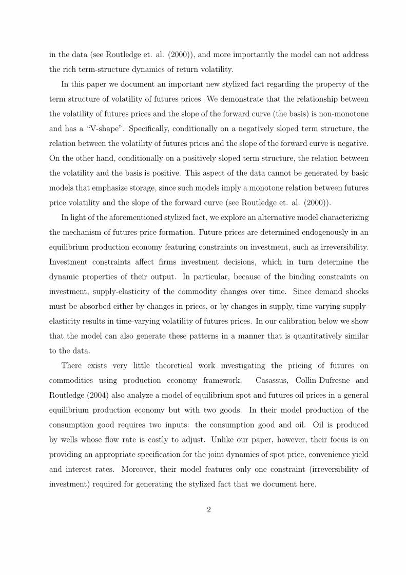
We first illustrate the fit of the model by plotting the term structure of unconditional futures

price volatility (to facilitate comparison with empirical data, we express our results as daily

values, defined as annual values scaled down by√

252). We chose model parameters, as

summarized in Table 4, to match the behavior of crude oil futures. Figure 7 compares

the volatility of prices implied by our choice of parameters to the empirical estimates. Our

model seems capable of reproducing the slow-decaying pattern of futures price volatility. This

feature of the data presents a challenge to simple storage models, as discussed in Routledge

et. al. (2000)). To see why it may not be easy to reproduce the slow-decaying pattern

of unconditional volatilities in a simple single-factor model, consider a reduced-form model

in which the logarithm of the spot price process follows a continuous-time AR(1) process

(Ornstein-Uhlenbeck process). Specifically, assume that the spot price is given by

St = eyt . (18)

and under the risk-neutral probability measure yt follows

dyt = θy(y − yt)dt + σydWt, (19)

where θy is the mean-reversion coefficient and y is the long-run mean of the state variable.

According to this simple model, the unconditional volatility of futures price changes is an

exponential function of maturity τ :

σ2(τ) = σ2ye−2θτ . (20)

To compare the term structure of unconditional volatility implied by this model to the one

generate by our model, we calibrate parameters θy and σy so that the simple model exhibits

the same volatility of the spot price and the same 30-day autocorrelation of the basis as

our model. Figure 7 shows that, as expected, unconditional volatility implied by the simple

model above decays too fast relative to our model and data.

The main qualitative distinction between the properties of our model and those of basic

storage models is in the conditional behavior of futures volatility. As we demonstrate in

Section 2, the empirical relation between the volatility of futures prices and the slope of the

13

term structure of prices is non-monotone and has a pronounced “V-shape”. Intuitively, we

would expect our model to exhibit this pattern. When the state variable ωt is far away from

the investment trigger ω∗, one of the investment constraints is binding and can be expected

to remain binding for some time. If the capital stock Kt is much higher than its optimal

level, given the current level of demand, firms find it optimal to postpone investment and

the irreversibility constraint binds. On the other hand, when Kt is much lower than the

optimal level, firms invest at the maximum possible rate and the investment rate constraint

binds. In either case, the supply of the commodity is relatively inelastic and futures prices

are relatively volatile. The further ωt travels away from the investment trigger, the larger

the effect on volatility of long-maturity futures. At the same time, it is precisely when ωt is

relatively far away from the investment trigger ω∗, when the absolute value of the slope of

the term structure of futures prices is large. This is to be expected. All prices in our model

are driven by a single mean-reverting stationary state variable, and since futures prices of

longer-maturity contracts are less sensitive to the current value of the state variable than

the spot price, the slope of the forward curve tends to be large when the state variable is far

away from its long-run average value. The latter, in turn, is not far from ω∗, given that ωt

reverts to ω∗. Thus, our model predicts that the volatility of futures prices should exhibit a

“V-shape” as a function of the slope of the term structure of futures prices.

It should be clear from the above discussion that the critical feature of the model is not

the precise definition of the production function, but rather the variable-elasticity property

of the supply side of the economy. The “V-shape” pattern in volatilities is due to the fact

that supply can adjust relatively easily in response to demand shocks when the output is

close to the optimal level, but supply is relatively inelastic when the output level is far from

the optimum.

We now report the quantitative properties of the model. The long-run average of the

slope of the forward curve, ln[

P (t−1,3)P (t−1,1)

], is 0.01 in the model, compared to the empirical

value of −0.0151. Both values are statistically indistinguishable from zero. The long-run

standard deviation of the slope in the model, which equals 0.0287, is slightly below the

empirical value of 0.0326. The 30-day autocorrelation coefficient of the slope implied by

the model is equal to 0.80, as compared to the value of 0.74 in the data. Overall, our

14

model fits the basic behavior of the slope of the forward curve quite well. Table 5 shows the

estimates of linear and piece-wise linear specifications of conditional variance of futures price

changes (2) implied by the model for one-, five-, and ten-month futures. The coefficients

of linear regressions are negative and close in magnitude to their empirical counterparts.

Such a negative relation between conditional volatility of futures prices and the basis would

typically be interpreted as supportive of simple storage models. Note, however, that our

model without storage can reproduce the same kind of relation. Our model, however, has a

further important implication: the linear model is badly misspecified, since the theoretically

predicted relation is non-monotone. Our piece-wise linear specification produces coefficients

β1,T and β2,T that agree with their empirical counterparts in sign but differ in magnitude.

Given the extremely streamlined nature of our model (e.g., the basis is a sufficient statistic

for conditional volatility), this should not be surprising. Also, it is important to keep in mind

that we did not target the volatility-basis relation in our estimation of structural parameters.

The entire distribution of regression coefficients across maturities of the futures contracts is

shown in Figure 8. Finally, Figure 9 helps visualize the “V-shape” pattern.

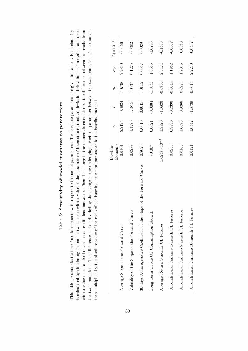
In order to understand the sensitivity of our results to the baseline parameters

summarized in Table 4, we compute elasticities of basic statistics of the model output with

respect to these parameters. Each elasticity is calculated by simulating the model twice:

with a value of the parameter of interest one standard deviation below (above) its baseline

value. Next, the change in the moment is calculated as the difference between the results

from the two simulations. This difference is then divided by the change in the underlying

structural parameter between the two simulations. Finally, the result is then multiplied by

the ratio of the baseline structural parameter to the baseline moment. The elasticities are

reported in Table 6.

An increase in the demand volatility, σY , or in the elasticity of the inverse demand curve,

γ, leads to an increase in the volatility of the spot price, which equals γ2σ2Y . As one would

expect, volatility of futures prices of various maturities increases as well. Qualitatively, both

of the parameters σY and γ affect the level of the unconditional volatility curve plotted in

Fig. 7. However, the demand volatility has strong positive effect on the expected growth

rate of oil consumption since it increases the long-run growth rate of the level of the demand

15

curve, Y −1t . γ has no such effect.

The constraint on the investment rate i has no effect on the volatility of the spot price.

However, it affects volatility of futures prices. A higher value of i allows capital stock to

adjust more rapidly in response to positive demand shocks, thus reducing the impact of

demand shocks on the future value of the spot price and therefore lowering the volatility

of futures prices. We thus see that i effectively controls the slope of the term structure of

volatility, higher values of i imply a steeper term structure. i has no effect on the expected

growth rate of oil consumption, in agreement with Eq. (17).

An increase in the unconditional mean of the demand shock, µY , has little affect on the

level of futures price volatility. This is not surprising given the role µY plays in the evolution

of the state variable ωt. An increase in µY raises the drift of ωt uniformly. The impact of this

on the volatility of futures price is ambiguous and depends on the relative magnitude of the

drift of ωt, µω, above and below the investment threshold ω∗. By symmetry considerations,

if µ+ = µ−, an infinitesimal change in µY has no impact on the volatility of futures prices.

Under the calibrated parameter values, µ− = 0.11 and µ+ = 0.08 and futures volatility is

not very sensitive to µY . The same is true for the risk premium, λ. Both µY and λ have

strong negative effect on gC in agreement with Eq. (17).

In general, the affect of model parameters on the slope of the forward curve is difficult to

interpret intuitively and depends on the chosen parameter values. However, the fact that the

moments of the slope have different sensitivities to various model parameters makes them

useful in estimating these parameters.

Finally, as a robustness check of our model we consider a possibility that a “V-shape”

in conditional volatility could arise mechanically due to heteroscedasticity in demand. We

therefore construct an alternative theoretical specification in which shocks to demand are

heteroscedastic, and their instantaneous volatility follows a continuous-time Markov process,

independent of other exogenous processes in the economy. We also assume that supply is

constant, while the level of demand is a mean-reverting stationary process. We find that not

to be the case – independent shocks to demand volatility cannot give rise to a non-monotone

relation between the slope of the forward curve and conditional volatility of futures prices.

Details of this analysis are presented in Appendix B.

16

5 Conclusions

This paper contributes along two dimensions. First, we show that volatility of future

prices has a “V-shape” relationship with respect to the slope of the term structure of

futures prices. Second, we show that such volatility patterns arise naturally in models

that emphasize investment constraints and, consequently, time-varying supply-elasticity as a

key mechanism for price dynamics. Our empirical findings seem beyond the scope of simple

storage models, which are currently the main focus of the literature, and point towards

investigating alternative economic mechanisms, such as the one analyzed in this paper.

Future work will entail a model that nests both storage and investment in an attempt to

isolate their quantitative effects.

17

References

Brennan, M., 1991, “The Price of Convenience and the Valuation of Commodity Contingent

Claims” in D. Lund and B. Oksendal (eds.), Stochastic Models and Option Models,

Elsevier Science Publishers, 1991.

Brennan, M. and E. Schwartz, 1985, “Evaluating Natural Resource Investments,” Journal

of Business 58, 135–157.

Casassus, J., P. Collin-Dufresne and B. Routledge, 2004, “Equilibrium Commodity Prices

with Irreversible Investment and Non-Linear Technologies”, CMU working paper.

Cooper, John C. B., 2003, “Price Elasticity of Demand for Crude Oil: Estimates for 23

Countries,” OPEC Review 27, 1-8.

Deaton, A. and G. Laroque, 1992, “On the Behavior of Commodity Prices,” The Review of

Financial Studies 59, 1–23.

Deaton, A. and G. Laroque, 1996, “Competitive Storage and Commodity Price Dynamics,”

Journal of Political Economy 104, 896–923.

Duffie, Darrell and Ken Singleton, 1993,“Simulated moments estimation of Markov models

of asset prices,” Econometrica 61, 929-952.

Gomes, Joao F., 2001, “Financing investment,” American Economic Review 91, 1263-1285.

Kaldor, N., 1939, “Speculation and Economic Stability,” The Review of Economic Studies

7, 1–27.

Kogan, L., 1999, Doctoral Dissertation, Sloan School of Management, MIT, Boston, MA.

Lee, B. and B. Ingram, 1991, “Simulation estimation of time series models”, Journal of

Econometrics 47, 197-205.

Lucas, R., and E. Prescott, 1971, “Investment under Uncertainty,” Econometrica 39, 659–

681.

18

Routledge, B., D. Seppi and C. Spatt, 2000, “Equilibrium Forward Curves for

Commodities,” Journal of Finance 55, 1297–1338.

Schwartz, E., 1997, “The Stochastic Behavior of Commodity Prices: Implications for

Valuation and Hedging,” Journal of Finance 52, 923–973.

Telser, L.G., 1958, “Futures Trading and the Storage of Cotton and Wheat,” Journal of

Political Economy 66, 133–144.

Williams, J. and B. Wright, 1991, Storage and Commodity Markets. Cambridge, England:

Cambridge University Press.

Working, H., 1948, “Theory of the Inverse Carrying Charge in Futures Markets,” Journal

of Farm Economics 30, 1–28.

Working, H., 1949, “The Theory of the Price of Storage,” American Economic Review 39,

1254–1262.

19

Appendix

A. Central Planner’s Problem

To characterize the solution of the social planner’s problem, we define the value function

J(Kt, Zt) as

J(Kt, Zt) = maxis∈[0,i]

Et

[∫ ∞

t

e−rf (s−t)

(Y −γ

s

K1−γs

1− γ− isKs

)ds

].

The Hamilton-Jacobi-Bellman (HJB) equation for J(Kt, Zt) takes the form

maxi∈[0,i]

[iKJK − iK] +σ2

Y

2Y 2JY Y + µY Y JY − δKJK + Y −γ K1−γ

1− γ− rfJ = 0. (A.1)

The solution to the above equation consists of the value function and endogenously

determined no-investment boundary determined by JK = 1. When JK ≥ 1 the investment

is made at a maximum rate i = i, and no investment is made when JK < 1.

We make the following change of variables in HJB equation

k = ln K, y = ln Y,

to obtain

maxit∈[0,i]

[iJk − ie−yek+y

]+

σ2Y

2Jyy + (µY −

σ2Y

2)Jy − δJk +

e−ye(1−γ)(k+y)

1− γ− rfJ = 0.

We will look for the solution in the form

J(k, y) =e−yf(ω)

1− γ, (A.2)

where ω = k + y. We have

Jk =e−yf ′

1− γ,

Jy =e−y

1− γ(f ′ − f) ,

Jyy =e−y

1− γ(f ′′ − 2f ′ + f) ,

and the ODE for f takes the form

maxi∈[0,i]

[if ′ − i (1− γ) eω] +σ2

Y

2f ′′ + (µY − δ− 3σ2

Y

2)f ′ + (σ2

Y − µY − rf )f + e(1−γ)ω = 0. (A.3)

20

We will look for a solution of (A.1) of the form

f(ω) =

{A exp(κ−(ω − ω∗)) + B exp((1− γ) ω), ω ≥ ω∗,

A exp(κ+(ω − ω∗)) + B exp((1− γ) ω) + C exp(ω), ω < ω∗,, (A.4)

for all γ’s, where ω∗ is the no-investment boundary in terms of the new state variable ω.

Substituting these solutions into ODE (A.3) yields quadratic equations on κ± and κ±σ2

Y

2κ2± − (δ +

3σ2Y

2− µY )κ± + (σ2

Y − µY − rf ) = 0, (A.5)

σ2Y

2κ2± − (δ − i +

3σ2Y

2− µY )κ± + (σ2

Y − µY − rf ) = 0,

and constants B, B, and C

B =1

rf + γµY + (1− γ)δ − γ(1+γ)2

σ2Y

, (A.6)

B =1

rf + γµY − (1− γ)(i− δ

)− γ(1+γ)2

σ2Y

,

C =(1− γ)i

i− δ.

For the quadratic equation on κ to have one negative root, we impose that

rf + µY − σ2Y > 0. (A.7)

As of now we have determined constants B, B, C, κ− and κ+, and we are left to

find four more parameters, constants A, A, and, finally, the no-investment boundary ω∗

in both cases. We have three boundary conditions to determine these constants. The first

two boundary conditions ensure continuity of f(ω) and its first derivative across the no-

investment boundary

f(ω∗ − 0) = f(ω∗ + 0), (A.8)

f ′(ω∗ − 0) = f ′(ω∗ + 0).

The investment optimality condition, JK = 1, which takes the following form in terms ω

f ′(ω∗) = (1− γ)eω∗ . (A.9)

is the third and the final one. Substituting equation (A.4) into the boundary conditions we

obtain the following system of equations

A− A =(B −B

)e(1−γ)ω∗ − Ceω∗

κ+A− κ−A = (1− γ)(B −B

)e(1−γ)ω∗ − Ceω∗

κ−A + (1− γ) Be(1−γ)ω∗ = (1− γ) eω∗, (A.10)

21

Solving last two equations in both systems we find the unique solution

A =κ+ + γ − 1

κ+ + |κ−|(B −B

)e(1−γ)ω∗ +

κ+ − 1

κ+ + |κ−|Ceω∗ , (A.11)

A =γ − |κ−| − 1

κ+ + |κ−|(B −B

)e(1−γ)ω∗ − |κ−|+ 1

κ+ + |κ−|Ceω∗ , (A.12)

eγω∗ =(1− γ + |κ−|)κ+B + (1− κ+) |κ−|B(1− γ) (κ+ + |κ−|) + |κ−| (κ+ − 1) C

.

B. Stationary long-run distribution of ωt

In this appendix we calculate the stationary long-run distribution of the state variable ω,

dynamics of which can be written as

dωt =[µ+1{ω≤ω∗} − µ−1{ω>ω∗}

]dt + σY dWt. (B.1)

The stationary distribution of ω

p(ω) =

{p+(ω) ω ≤ ω∗

p−(ω) ω > ω∗, (B.2)

exists if 0 < µ− < i and it satisfies backward Kolmogorov ODE

d2p(ω)

dω2− 2

[µ+1{ω≤ω∗} − µ−1{ω>ω∗}

]

σ2Y

dp(ω)

dω= 0. (B.3)

p(ω) also satisfies the normalization condition

∫ ω∗

−∞p+(ω)dω +

∫ ∞

ω∗p−(ω)dω = 1. (B.4)

Condition (B.4) eliminates a constant as a trivial solution of the ODE (B.3) which can be

integrated once to yield

dp(ω)

dω− 2

[µ+1{ω≤ω∗} − µ−1{ω>ω∗}

]

σ2Y

p(ω) = 0. (B.5)

We can find necessary boundary condition at ω = ω∗ by integrating equation (B.5) over the

interval ω ∈ [ω∗ − ε, ω∗ + ε] and then taking limit of ε → 0

limε→0

∫ ω∗+ε

ω∗−ε

[dp(ω)

dω− 2

[µ+1{ω≤ω∗} − µ−1{ω>ω∗}

]

σ2Y

p(ω)

]dω = p−(ω∗)− p+(ω∗) = 0. (B.6)

22

Therefore, we obtain that p(ω) is continuous at ω = ω∗. We can now solve ODE (B.3)

separately for p+(ω) and p−(ω)

p+(ω) = A+e2µ+

σ2Y

ω, (B.7)

p−(ω) = A−e− 2µ−

σ2Y

ω,

where A± can be found from the boundary and normalization conditions which take the

following forms

A+e2µ+

σ2Y

ω∗= A−e

− 2µ−σ2

Y

ω∗, (B.8)

σ2Y

2µ+A+e

2µ+

σ2Y

ω∗+

σ2Y

2µ−A−e

− 2µ−σ2

Y

ω∗= 1.

Solving equations (B.8) we finally obtain Eq. (11).

C. Robustness Check

In this appendix we analyze a simple economy with heteroscedastic shocks to the level of the

demand curve. Our objective is to establish that the “V-shape” of the conditional volatility

of futures prices implied by our production-based model does not arise spuriously simply due

to heteroscedasticity in demand shocks. An informal argument would suggest that such a

possibility exists. If demand shocks have time-varying volatility, one could expect the slope

of the forward curve to move further away from its long-run mean when conditional volatility

of demand shocks is relatively high, thus giving rise to a ‘V-shaped’ relation observed in the

data. The above argument is informal because it makes an implicit connection between the

volatility of demand shocks and the volatility of the slope of the forward curve, meanwhile

assuming that the conditional mean of the slope is unaffected by changes in demand shock

volatility. Below we develop a simple explicit model and show that heteroscedasticity of

demand shocks does not immediately lead to a convex relation between the conditional

futures price volatility and the slope of the demand curve.

Our model here is similar to the main model in the paper. As before, consumers

represented by the demand curve

Qt = Y −1t S

− 1γ

t , (C.1)

23

where unexpected changes in Yt represent demand shocks. The most significant departure

from the earlier formulation is the simplifying assumption that the level of supply is fixed at

Q = eq. To make sure that prices are stationary, we assume that the level of demand curve

yt = ln Yt follows a linear mean-reverting process

dyt = θ(y − yt)dt + σtdWt, (C.2)

The conditional volatility of the demand process is stochastic, it follows a continuous

Markov process independent of Wt. The precise functional form of the volatility process is

not important for our results.

In equilibrium, supply equals demand and hence the spot price is equal to

St = e−γ(yt+q), (C.3)

while futures price is equal to

P (t, T ) = Et[ST ] = e−γqEt[e−γyT ], ∀T ≥ 0. (C.4)

We now characterize futures prices analytically. Notice that since the process for volatility

is independent of demand shocks, we can first calculate the expectation over Wt, treating

the process σt as deterministic, and then calculate the expectation over σt.

The solution for yT is standard:

yT = ytZ(t) + y(1− Z(t)) +

∫ T

t

Z(s)σsdWs, (C.5)

where Z(t) ≡ e−θ(T−t). Taking expectations over Wt we find that futures prices are given by

P (t, T ) = SZ(t)t e−γ(y+q)(1−Z(t))E

[exp

{γ2

2

∫ T

t

Z2(s)σ2sds

}|σt

]. (C.6)

It is easy to see that the conditional volatility of futures prices of all maturities is equal

to σt. The slope of the forward curve is given by

P (t, T )

St

= SZ(t)−1t e−γ(y+q)(1−Z(t))E

[exp

{γ2

2

∫ T

t

Z2(s)σ2sds

}|σt

]. (C.7)

Because the volatility process σt is continuous and Markov, the conditional expectation in

the previous expression is increasing in σt. Thus, we find that the conditional volatility

of futures prices is positively related to slope of the term structure, in contrast to a non-

monotone convex relation implied by the main model in the paper.

24

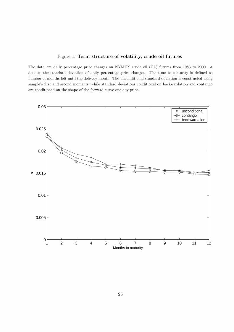
Figure 1: Term structure of volatility, crude oil futures

The data are daily percentage price changes on NYMEX crude oil (CL) futures from 1983 to 2000. σ

denotes the standard deviation of daily percentage price changes. The time to maturity is defined asnumber of months left until the delivery month. The unconditional standard deviation is constructed usingsample’s first and second moments, while standard deviations conditional on backwardation and contangoare conditioned on the shape of the forward curve one day prior.

1 2 3 4 5 6 7 8 9 10 11 120

0.005

0.01

0.015

0.02

0.025

0.03

Months to maturity

σ

unconditionalcontangobackwardation

25

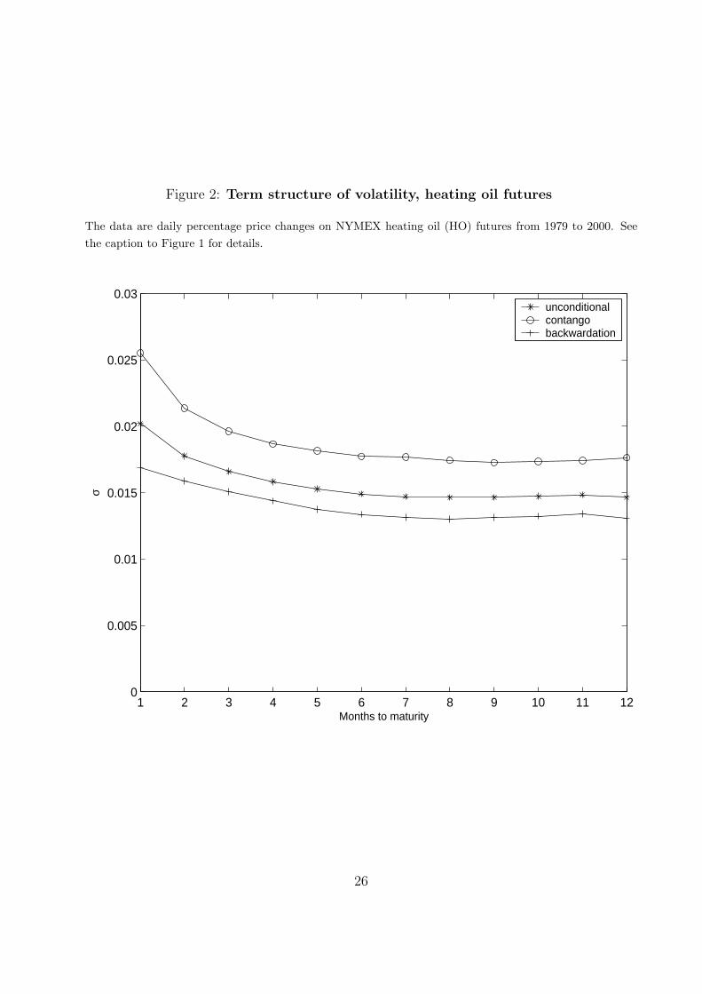
Figure 2: Term structure of volatility, heating oil futures

The data are daily percentage price changes on NYMEX heating oil (HO) futures from 1979 to 2000. Seethe caption to Figure 1 for details.

1 2 3 4 5 6 7 8 9 10 11 120

0.005

0.01

0.015

0.02

0.025

0.03

Months to maturity

σ

unconditionalcontangobackwardation

26

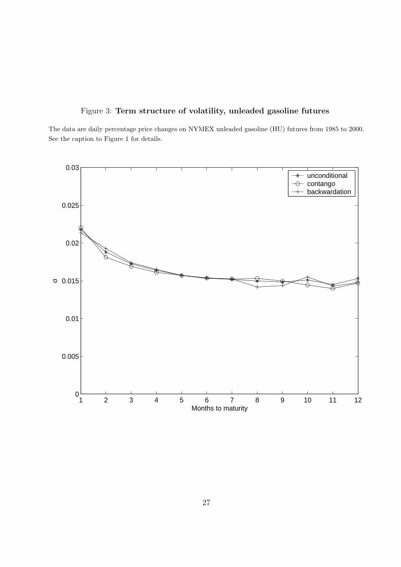
Figure 3: Term structure of volatility, unleaded gasoline futures

The data are daily percentage price changes on NYMEX unleaded gasoline (HU) futures from 1985 to 2000.See the caption to Figure 1 for details.

1 2 3 4 5 6 7 8 9 10 11 120

0.005

0.01

0.015

0.02

0.025

0.03

Months to maturity

σ

unconditionalcontangobackwardation

27

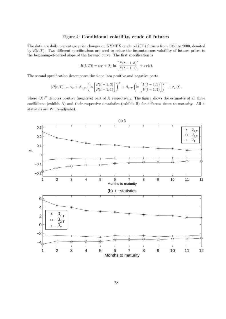
Figure 4: Conditional volatility, crude oil futures

The data are daily percentage price changes on NYMEX crude oil (CL) futures from 1983 to 2000, denotedby R(t, T ). Two different specifications are used to relate the instantaneous volatility of futures prices tothe beginning-of-period slope of the forward curve. The first specification is

|R(t, T )| = αT + βT ln[P (t− 1, 3)P (t− 1, 1)

]+ εT (t).

The second specification decomposes the slope into positive and negative parts

|R(t, T )| = αT + β1,T

(ln

[P (t− 1, 3)P (t− 1, 1)

])+

+ β2,T

(ln

[P (t− 1, 3)P (t− 1, 1)

])−+ εT (t),

where (X)± denotes positive (negative) part of X respectively. The figure shows the estimates of all threecoefficients (exhibit A) and their respective t-statistics (exhibit B) for different times to maturity. All t-statistics are White-adjusted.

1 2 3 4 5 6 7 8 9 10 11 12

−0.2

−0.1

0

0.1

0.2

0.3

(a) β

Months to maturity

β

1 2 3 4 5 6 7 8 9 10 11 12

−4

−2

0

2

4

6

(b) t −statistics

Months to maturity

β1,T

β2,T

βT

β1,T

β2,T

βT

28

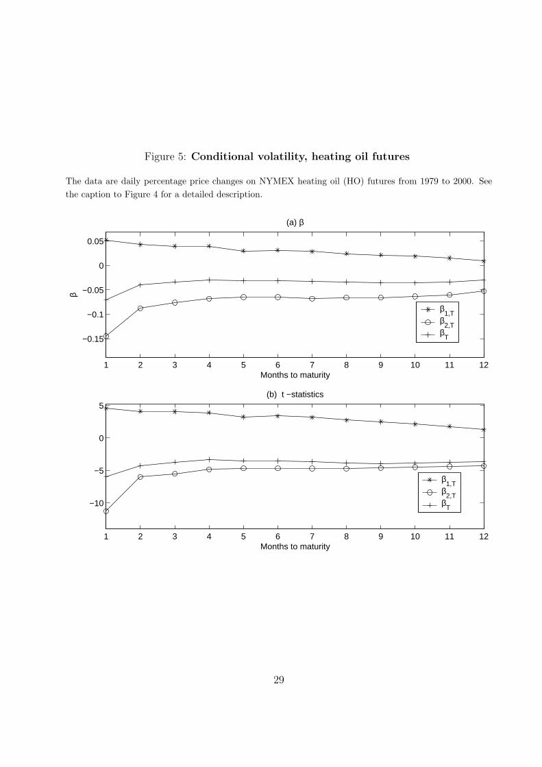
Figure 5: Conditional volatility, heating oil futures

The data are daily percentage price changes on NYMEX heating oil (HO) futures from 1979 to 2000. Seethe caption to Figure 4 for a detailed description.

1 2 3 4 5 6 7 8 9 10 11 12

−0.15

−0.1

−0.05

0

0.05

(a) β

Months to maturity

β

β1,T

β2,T

βT

1 2 3 4 5 6 7 8 9 10 11 12

−10

−5

0

5(b) t −statistics

Months to maturity

β1,T

β2,T

βT

29

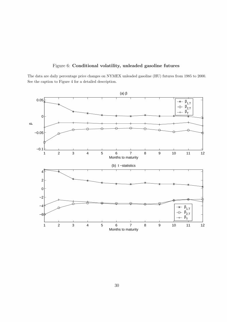
Figure 6: Conditional volatility, unleaded gasoline futures

The data are daily percentage price changes on NYMEX unleaded gasoline (HU) futures from 1985 to 2000.See the caption to Figure 4 for a detailed description.

1 2 3 4 5 6 7 8 9 10 11 12−0.1

−0.05

0

0.05

(a) β

Months to maturity

β

β1,T

β2,T

βT

1 2 3 4 5 6 7 8 9 10 11 12

−6

−4

−2

0

2

4

(b) t −statistics

Months to maturity

β1,T

β2,T

βT

30

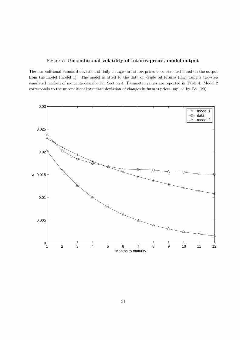
Figure 7: Unconditional volatility of futures prices, model output

The unconditional standard deviation of daily changes in futures prices is constructed based on the outputfrom the model (model 1). The model is fitted to the data on crude oil futures (CL) using a two-stepsimulated method of moments described in Section 4. Parameter values are reported in Table 4. Model 2corresponds to the unconditional standard deviation of changes in futures prices implied by Eq. (20).

1 2 3 4 5 6 7 8 9 10 11 120

0.005

0.01

0.015

0.02

0.025

0.03

Months to maturity

σ

model 1datamodel 2

31

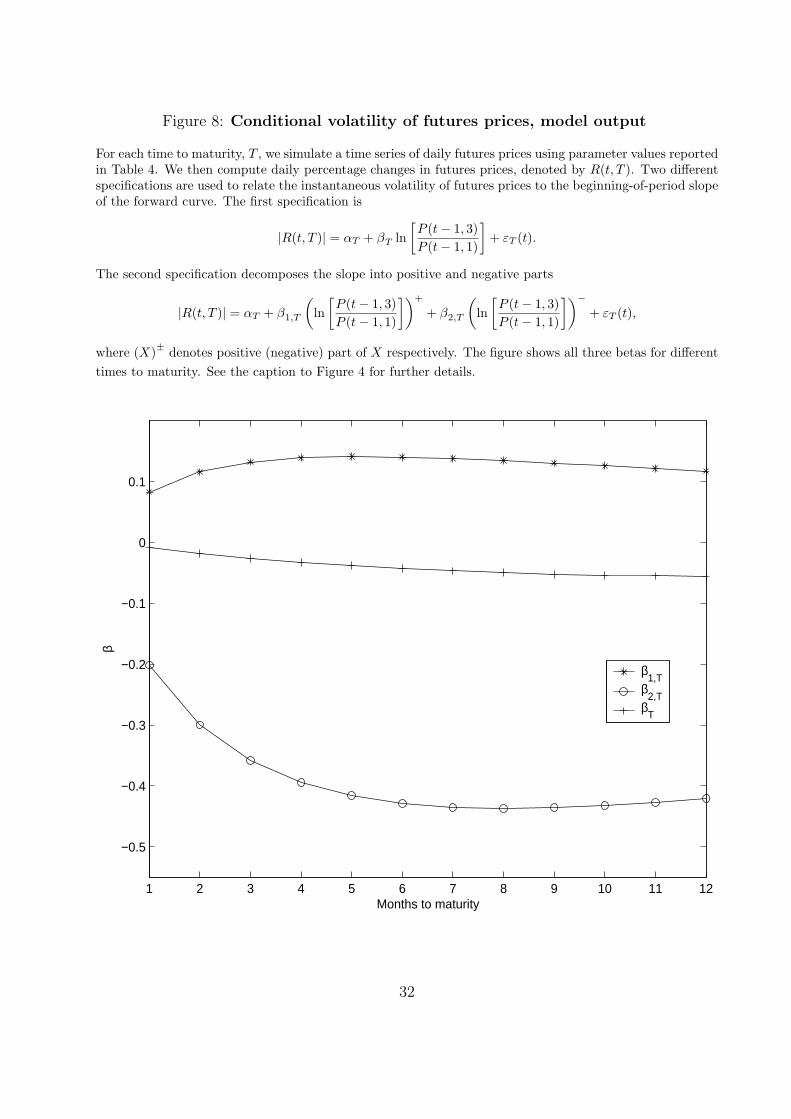
Figure 8: Conditional volatility of futures prices, model output

For each time to maturity, T , we simulate a time series of daily futures prices using parameter values reportedin Table 4. We then compute daily percentage changes in futures prices, denoted by R(t, T ). Two differentspecifications are used to relate the instantaneous volatility of futures prices to the beginning-of-period slopeof the forward curve. The first specification is

|R(t, T )| = αT + βT ln[P (t− 1, 3)P (t− 1, 1)

]+ εT (t).

The second specification decomposes the slope into positive and negative parts

|R(t, T )| = αT + β1,T

(ln

[P (t− 1, 3)P (t− 1, 1)

])+

+ β2,T

(ln

[P (t− 1, 3)P (t− 1, 1)

])−+ εT (t),

where (X)± denotes positive (negative) part of X respectively. The figure shows all three betas for differenttimes to maturity. See the caption to Figure 4 for further details.

1 2 3 4 5 6 7 8 9 10 11 12

−0.5

−0.4

−0.3

−0.2

−0.1

0

0.1

Months to maturity

β

β1,T

β2,T

βT

32

Figure 9: Properties of volatility of futures prices, model output

The figure reports the model’s term structure of futures volatility with respect to time of maturity and theslope of the forward curve. Volatility is expressed in annual terms.

−0.04−0.02

00.02

0.040.06

0.080.1

0.2

0.4

0.6

0.8

10.05

0.1

0.15

0.2

0.25

0.3

0.35

0.4

0.45

Slope of term structureTime to maturity

Vo

latil

ity o

f fu

ture

s p

rice

33

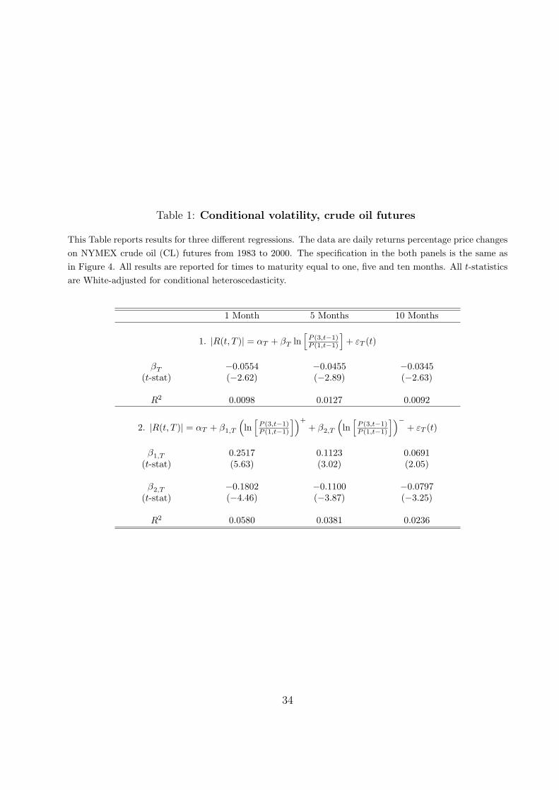
Table 1: Conditional volatility, crude oil futures

This Table reports results for three different regressions. The data are daily returns percentage price changeson NYMEX crude oil (CL) futures from 1983 to 2000. The specification in the both panels is the same asin Figure 4. All results are reported for times to maturity equal to one, five and ten months. All t-statisticsare White-adjusted for conditional heteroscedasticity.

1 Month 5 Months 10 Months

1. |R(t, T )| = αT + βT ln[

P (3,t−1)P (1,t−1)

]+ εT (t)

βT

(t-stat)

R2

−0.0554(−2.62)

0.0098

−0.0455(−2.89)

0.0127

−0.0345(−2.63)

0.0092

2. |R(t, T )| = αT + β1,T

(ln

[P (3,t−1)P (1,t−1)

])+

+ β2,T

(ln

[P (3,t−1)P (1,t−1)

])−+ εT (t)

β1,T

(t-stat)

β2,T

(t-stat)

R2

0.2517(5.63)

−0.1802(−4.46)

0.0580

0.1123(3.02)

−0.1100(−3.87)

0.0381

0.0691(2.05)

−0.0797(−3.25)

0.0236

34

Table 2: Conditional volatility, heating oil futures

This table reports results for three different regressions. The data are daily percentage price changes onNYMEX heating oil (HO) futures from 1979 to 2000. See the caption to Table 1.

1 Month 5 Months 10 Months

1. |R(t, T )| = αT + βT ln[

P (3,t−1)P (1,t−1)

]+ εT (t)

βT

(t-stat)

R2

−0.0711(−5.97)

0.0388

−0.0309(−3.51)

0.0140

−0.0359(−3.89)

0.0189

2. |R(t, T )| = αT + β1,T

(ln

[P (3,t−1)P (1,t−1)

])+

+ β2,T

(ln

[P (3,t−1)P (1,t−1)

])−+ εT (t)

β1,T

(t-stat)

β2,T

(t-stat)

R2

0.0523(4.54)

−0.1450(−10.8)

0.0722

0.0300(3.21)

−0.0646(−4.65)

0.0473

0.0192(2.14)

−0.0632(−4.27)

0.0286

35

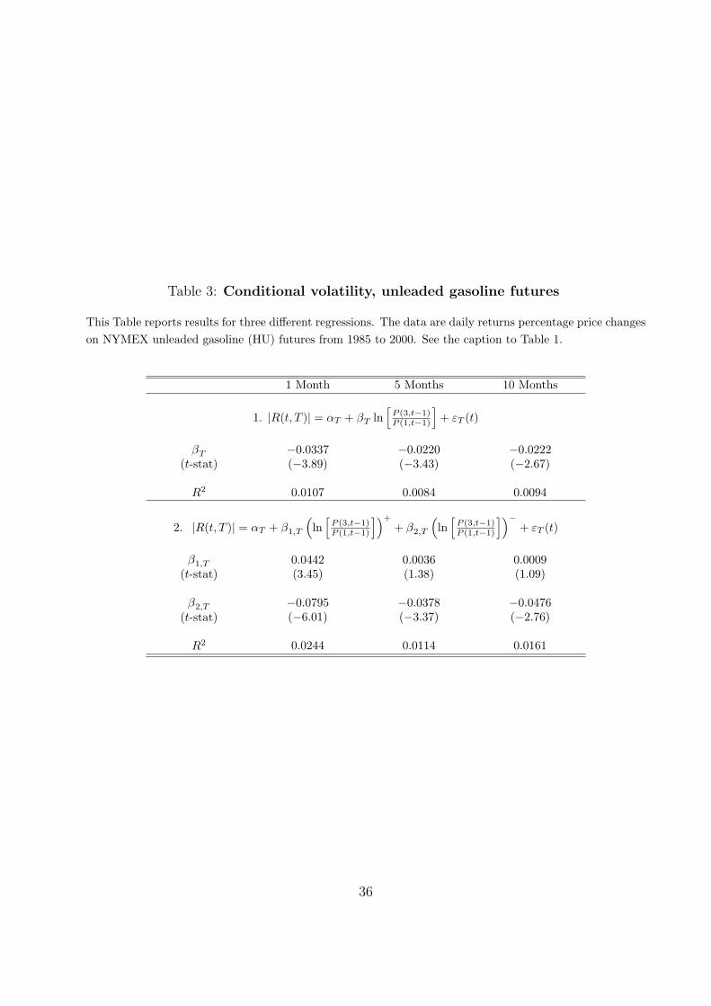
Table 3: Conditional volatility, unleaded gasoline futures

This Table reports results for three different regressions. The data are daily returns percentage price changeson NYMEX unleaded gasoline (HU) futures from 1985 to 2000. See the caption to Table 1.

1 Month 5 Months 10 Months

1. |R(t, T )| = αT + βT ln[

P (3,t−1)P (1,t−1)

]+ εT (t)

βT

(t-stat)

R2

−0.0337(−3.89)

0.0107

−0.0220(−3.43)

0.0084

−0.0222(−2.67)

0.0094

2. |R(t, T )| = αT + β1,T

(ln

[P (3,t−1)P (1,t−1)

])+

+ β2,T

(ln

[P (3,t−1)P (1,t−1)

])−+ εT (t)

β1,T

(t-stat)

β2,T

(t-stat)

R2

0.0442(3.45)

−0.0795(−6.01)

0.0244

0.0036(1.38)

−0.0378(−3.37)

0.0114

0.0009(1.09)

−0.0476(−2.76)

0.0161

36

Table 4: Parameter estimates, crude oil futures

This table reports our parameter values. We use a two step SMM procedure to estimate vector of sevenstructural parameters θ ≡ {γ, µY , σY , i, rf , δ, λ}. Since only five model parameters can be independentlyidentified from the data (see Section 4), we fix δ and r and estimate the remaining five parameters. We matchthe unconditional properties of futures prices, specifically the historic daily return on fully collateralizedthree-month futures position, the unconditional volatility of daily percent price changes for futures of variousmaturities as well as the mean, volatility, and the 30-day autoregressive coefficient of the slope of the forwardcurve. We use crude oil futures prices as a benchmark. In addition, we match the expected growth rate ofcrude oil consumption. The standard errors are reported where applicable.

Parameter Value Std. Error

γ 3.9221 0.0587

i 0.1904 0.0073

rf 0.0200 NA

µY 0.0124 0.0055

σY 0.1036 0.0108

δ 0.1200 NA

λ 1.5×10−5 0.0016

37

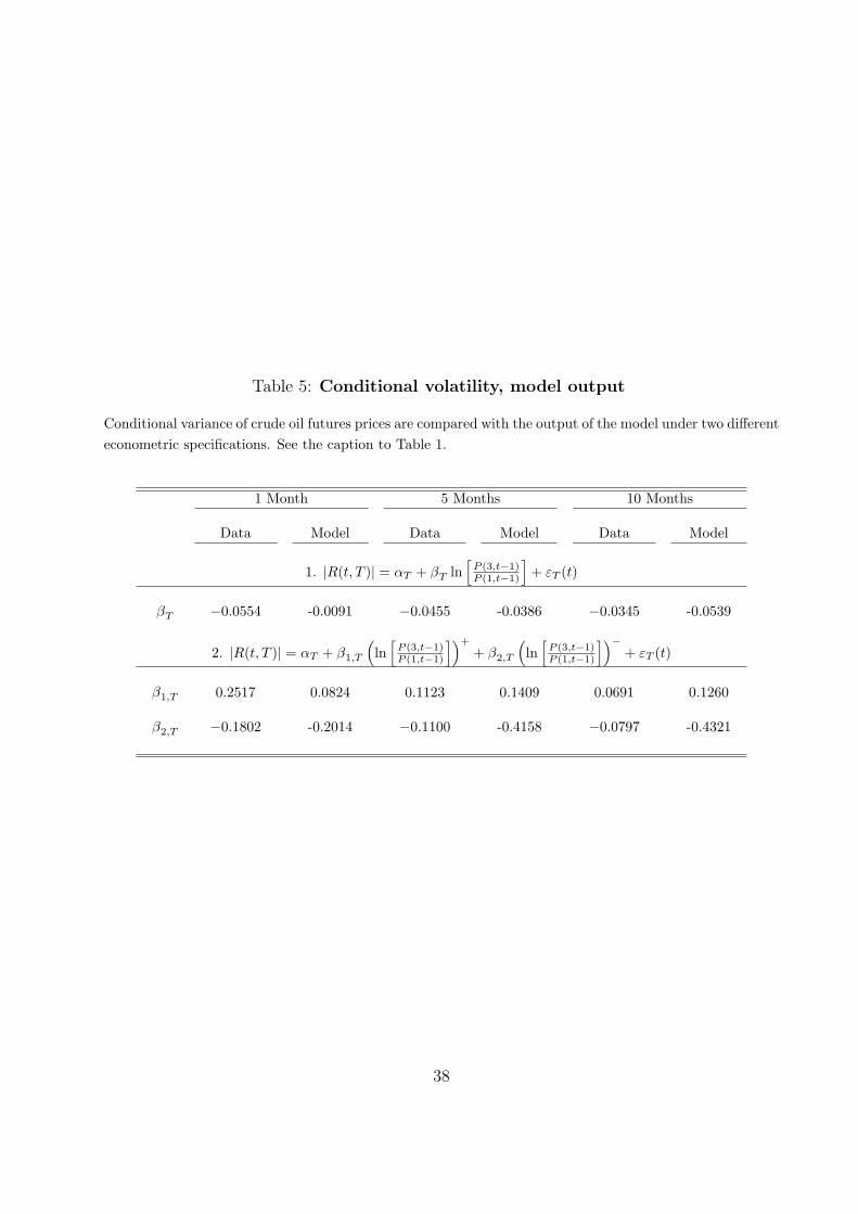
Table 5: Conditional volatility, model output

Conditional variance of crude oil futures prices are compared with the output of the model under two differenteconometric specifications. See the caption to Table 1.

1 Month 5 Months 10 Months

Data Model Data Model Data Model

1. |R(t, T )| = αT + βT ln[

P (3,t−1)P (1,t−1)

]+ εT (t)

βT −0.0554 -0.0091 −0.0455 -0.0386 −0.0345 -0.0539

2. |R(t, T )| = αT + β1,T

(ln

[P (3,t−1)P (1,t−1)

])+

+ β2,T

(ln

[P (3,t−1)P (1,t−1)

])−+ εT (t)

β1,T

β2,T

0.2517

−0.1802

0.0824

-0.2014

0.1123

−0.1100

0.1409

-0.4158

0.0691

−0.0797

0.1260

-0.4321

38

Tab

le6:

Sensi

tivity

ofm

odelm

om

ents

topara

mete

rs

Thi

sta

ble

pres

ents

elas

tici

ties

ofm

odel

mom

ents

wit

hre

spec

tto

the

mod

elpa

ram

eter

s.T

heba

selin

epa

ram

eter

sar

egi

ven

inTab

le4.

Eac

hel

asti

city

isca

lcul

ated

bysi

mul

atin

gth

em

odel

twic

e:on

cew

ith

ava

lue

ofth

epa

ram

eter

ofin

tere

ston

est

anda

rdde

viat

ion

belo

wit

sba

selin

eva

lue,

and

once

wit

ha

valu

eon

est

anda

rdde

viat

ion

abov

eit

sba

selin

eva

lue.

The

nth

ech

ange

inth

em

omen

tis

calc

ulat

edas

the

diffe

renc

ebe

twee

nth

ere

sult

sfr

omth

etw

osi

mul

atio

ns.

Thi

sdi

ffere

nce

isth

endi

vide

dby

the

chan

gein

the

unde

rlyi

ngst

ruct

ural

para

met

erbe

twee

nth

etw

osi

mul

atio

ns.

The

resu

ltis

then

mul

tipl

ied

byth

eab

solu

teva

lue

ofth

era

tio

ofth

eba

selin

est

ruct

ural

para

met

erto

the

base

line

mom

ent.

Bas

elin

eM

omen

tsγ

iµ

Yσ

Yλ(×

10−

3)

Ave

rage

Slop

eof

the

Forw

ard

Cur

ve0.

0101

2.21

24-0

.692

40.

0738

2.28

500.

6456

Vol

atili

tyof

the

Slop

eof

the

Forw

ard

Cur

ve0.

0287

1.12

761.

1893

0.05

370.

1225

0.03

82

30-d

ays

Aut

oreg

ress

ive

Coe

ffici

ent

ofth

eSl

ope

ofth

eFo

rwar

dC

urve

0.80

260.

0616

0.00

130.

0115

0.05

370.

0029

Lon

gTer

mC

rude

Oil

Con

sum

ptio

nG

row

th-0

.007

0.00

21-0

.000

4-1

.804

61.

5635

-1.6

785

Ave

rage

Ret

urn

3-m

onth

CL

Futu

res

1.02

47×1

0−4

1.99

20-1

.082

6-0

.073

82.

3424

-0.1

588

Unc

ondi

tion

alV

aria

nce

1-m

onth

CL

Futu

res

0.02

300.

9930

-0.2

396

-0.0

044

1.19

32-0

.003

2

Unc

ondi

tion

alV

aria

nce

5-m

onth

CL

Futu

res

0.01

661.

0025

-0.9

266

-0.0

274

1.70

75-0

.024

9

Unc

ondi

tion

alV

aria

nce

10-m

onth

CL

Futu

res

0.01

211.

0447

-1.6

739

-0.0

613

2.22

10-0

.046

7

39