FUSING AND COMPOSING MACROMOLECULAR REGULATORYNETWORK MODELS

Ranjit Randhawa∗, Clifford A. Shaffer∗, and John J. Tyson∗∗

Departments of Computer Science∗ and Biological Sciences∗∗Virginia Tech

Blacksburg, VA 24061rrandhawa|shaffer|tyson@vt.edub

Keywords: Computational Biology, Systems BiologyMarkup Language (SBML), pathway models

AbstractToday’s macromolecular regulatory network models aresmall compared to the amount of information known aboutthe corresponding cellular pathways, in part because currentmodeling languages and tools are unable to handle signifi-cantly larger models. Most pathway models are small modelsof individual pathways which are relatively easy to constructand manage. The hope is someday to put these pieces togetherto create a more complete picture of the underlying molecu-lar machinery. While efforts to make large models can benefitfrom reusing existing components, there currently exists littletool or representational support for combining or composingmodels. In this paper we present a tool for merging two ormore models (we call this process model fusion) and a con-crete proposal for implementing composition in the contextof the Systems Biology Markup Language (SBML).

REGULATORY NETWORK MODELINGMacromolecular regulatory network models attempt to de-

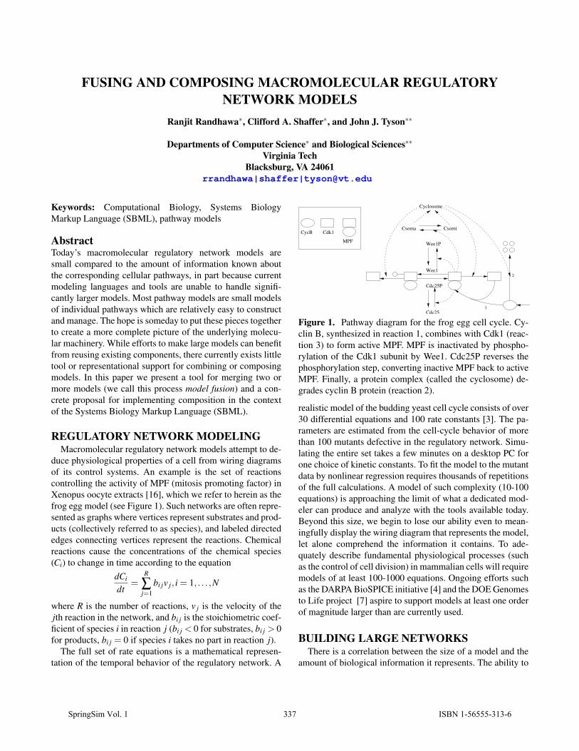
duce physiological properties of a cell from wiring diagramsof its control systems. An example is the set of reactionscontrolling the activity of MPF (mitosis promoting factor) inXenopus oocyte extracts [16], which we refer to herein as thefrog egg model (see Figure 1). Such networks are often repre-sented as graphs where vertices represent substrates and prod-ucts (collectively referred to as species), and labeled directededges connecting vertices represent the reactions. Chemicalreactions cause the concentrations of the chemical species(Ci) to change in time according to the equation

dCi

dt=

R

∑j=1

bi jv j, i = 1, . . . ,N

where R is the number of reactions, v j is the velocity of thejth reaction in the network, and bi j is the stoichiometric coef-ficient of species i in reaction j (bi j < 0 for substrates, bi j > 0for products, bi j = 0 if species i takes no part in reaction j).

The full set of rate equations is a mathematical represen-tation of the temporal behavior of the regulatory network. A

CycB Cdk1MPF

CsomiCsoma

Cyclosome

1

2

3

Wee1

Cdc25P

Wee1P

Cdc25

Figure 1. Pathway diagram for the frog egg cell cycle. Cy-clin B, synthesized in reaction 1, combines with Cdk1 (reac-tion 3) to form active MPF. MPF is inactivated by phospho-rylation of the Cdk1 subunit by Wee1. Cdc25P reverses thephosphorylation step, converting inactive MPF back to activeMPF. Finally, a protein complex (called the cyclosome) de-grades cyclin B protein (reaction 2).

realistic model of the budding yeast cell cycle consists of over30 differential equations and 100 rate constants [3]. The pa-rameters are estimated from the cell-cycle behavior of morethan 100 mutants defective in the regulatory network. Simu-lating the entire set takes a few minutes on a desktop PC forone choice of kinetic constants. To fit the model to the mutantdata by nonlinear regression requires thousands of repetitionsof the full calculations. A model of such complexity (10-100equations) is approaching the limit of what a dedicated mod-eler can produce and analyze with the tools available today.Beyond this size, we begin to lose our ability even to mean-ingfully display the wiring diagram that represents the model,let alone comprehend the information it contains. To ade-quately describe fundamental physiological processes (suchas the control of cell division) in mammalian cells will requiremodels of at least 100-1000 equations. Ongoing efforts suchas the DARPA BioSPICE initiative [4] and the DOE Genomesto Life project [7] aspire to support models at least one orderof magnitude larger than are currently used.

BUILDING LARGE NETWORKSThere is a correlation between the size of a model and the

amount of biological information it represents. The ability to

SpringSim Vol. 1 337 ISBN 1-56555-313-6

construct large biological models provides the potential forbetter insights into the workings of a cell under investiga-tion, if only we can handle the complexity involved. Modelsthat exist today are small compared to the amount of infor-mation known about the corresponding organism or cellularpathway/process, on the order of 10s of species and/or reac-tions. Modelers work on individual pieces (cellular processesor certain pathways) that are easy to construct and manage.Their ultimate goal is to put these pieces together, increasingthe size and complexity by an order of magnitude, to con-struct a more complete picture of the underlying molecularmachinery of the organism. Merging the pieces together willprovide researchers with more complete and biologically ac-curate models with which to perform simulations. Currentlythis merging step is an error-prone process since it is donemanually. The level of complexity is difficult to deal withas the number of models and their sizes increase. Efficientlyrunning simulations and parameter estimation for models be-comes even more of a concern as model size and complexityincrease. Our work is intended to be a first step for scaling upto larger problems. When making large models it is helpful tostart from existing models and reuse information, rather thanstart from scratch. Using existing models also ensures that thenewly created model will be consistent with the experimentaldata. One can assume that each of the submodels used in cre-ating the larger model is in fact a validated model with experi-mental data that fixes its parameters. The main motivation forcreating larger models is because there exists new data thatthe current (sub)models cannot explain or describe. A simpleyet effective method to verify the biological accuracy of thenewly created model is to ensure that it is consistent with boththe older submodel data as well as the new data.

Modeling languages and tools help modelers constructtheir models by providing a computational environment thatminimizes the amount of human error during the construc-tion step. While modelers are currently able to construct smallto medium models by hand, the process is simplified by us-ing computational tools which not only decrease the timetaken to input a model but also ensure that the modeler doesnot make mistakes while inputting the model. In this paperwe describe techniques that are intended to enable modelersto create larger models than previously possible. Our priorwork has identified a number of modeling processes relatedto model composition [18]. In this paper we describe two dis-tinct modeling processes whose purpose is to support the con-struction of larger models: Fusion and Composition.

Model Fusion is a process that combines two or more mod-els in an irreversible manner. In fusion, the identities of the in-dividual models (called submodels) being combined are lost,but the aggregated information remains the same. Fusion en-ables modelers to incorporate information from one modelinto another model, thereby creating larger models. Eventu-

ally, fused models will become too large to grasp and man-age as single entities. Large models will ultimately need to bemade up of distinct components to infer any meaningful in-sight into their underlying biology. Thus, while model fusionas a useful tool for manipulating small to mid-sized models,it is not a viable solution in the long run.

Model Composition provides a potential solution to ourlimited ability to comprehend larger pathway models. Withcomposition, one can think of models not as monolithic en-tities, but as collections of smaller components (submodels)joined together. A composed model is built from two or moresubmodels by describing their redundancies and interactions.Composition is a reversible process, in that removing theinter-model interaction description that holds the composedmodel together recovers the individual submodels.

CONTEXT AND PRIOR WORKThe XML-based Systems Biology Markup Language

(SBML) [9, 12] has become widely supported within thepathway modeling community. Thus, we choose to presentconcrete implementations for the various modeling processesthrough added SBML language constructs that express thenecessary glue that connects submodels together. It is not nec-essary that our proposals be implemented in SBML, but doingso provides clear reference implementations in the same wayas an algorithm expressed in a particular programming lan-guage. Fusion is presented in terms of a tool to aid modelershand compose large models from smaller components.

A number of authors find that successful composition orreuse requires components that were designed for the pur-pose [5, 10, 13, 15, 19]. Bulatewicz, et al. [2] suggest usinga coupling interface for model coupling and provide a num-ber of solutions, from a brute force technique to using frame-works designed to support coupling. Liang and Paredis [14]describe a port ontology for automated model composition.While automating composition is outside the scope of ourwork, the ontology for representing ports is useful in detailingthe different roles and functions port structures can take.

Proposals have been made within the SBML commu-nity [8, 11, 17] that describe the mechanics of compositionthrough additional language features for SBML, as we willdo. However, we note that none of these proposals have beenpublished in the peer-reviewed literature, nor to our knowl-edge have any been implemented. While some commercialtools might have more or less support for various forms ofcomposition, we are unaware of any non-proprietary imple-mentations for model composition in this application domain,or any publications describing proprietary features in com-mercial applications. Model composition for pathway modelsremains very much an open problem.

ISBN 1-56555-313-6 338 SpringSim Vol. 1

MODEL FUSIONModel Fusion is an iterative process to make larger models

by merging two or more submodels together. Unlike com-position (where submodels are referenced but not modified),fusion takes the the submodels and actually makes changes tothem as part of the process of combining them together. Thegoal of fusion is to combine submodels into a single unifiedmodel containing all the information of the original collec-tion, without any redundancies that might occur across sub-models in the original collection. Our approach to fusion isto provide tools that aid modelers attempting to perform thefusion process.

Sample modelsThe chromosome cycle is divided into four phases (G1,

S, G2 and M), with two irreversible transitions (Start andFinish). The two transitions are irreversible due to the cre-ation and destruction of stable steady states of the molecu-lar regulatory mechanism by dynamic bifurcations [1, 20]. Anetwork of molecular signals control events in the cell cycle(cyclin-dependent protein kinases). The Start transition sep-arates G1 from S; once the cell passes this transition it com-mits itself to DNA synthesis. Start is triggered by the proteinkinase, Cdk (referred to using its cyclin partner CycB in thesample models). At Start, cyclin synthesis is induced and cy-clin degradation is inhibited. This causes a rise in Cdk activ-ity which is needed for DNA synthesis. The Finish transitionseparates M from G1, and occurs when DNA replication iscomplete. Once the cell enters the Finish transition, it com-mits itself to cell division. Finish is accomplished by activat-ing a group of proteins that make up the anaphase-promotingcomplex (APC; also known as the cyclosome), which labelsspecific proteins for degradation. The APC contains two aux-iliary proteins, Cdc20 and Cdh1, whose role (when active) isto recognize cyclins and present them to the complex for la-beling (and degradation), which allows the system to returnto G1. Cdc20 and Cdh1 are controlled differently by cyclin-Cdk, which activates Cdc20 and inhibits Cdh1.

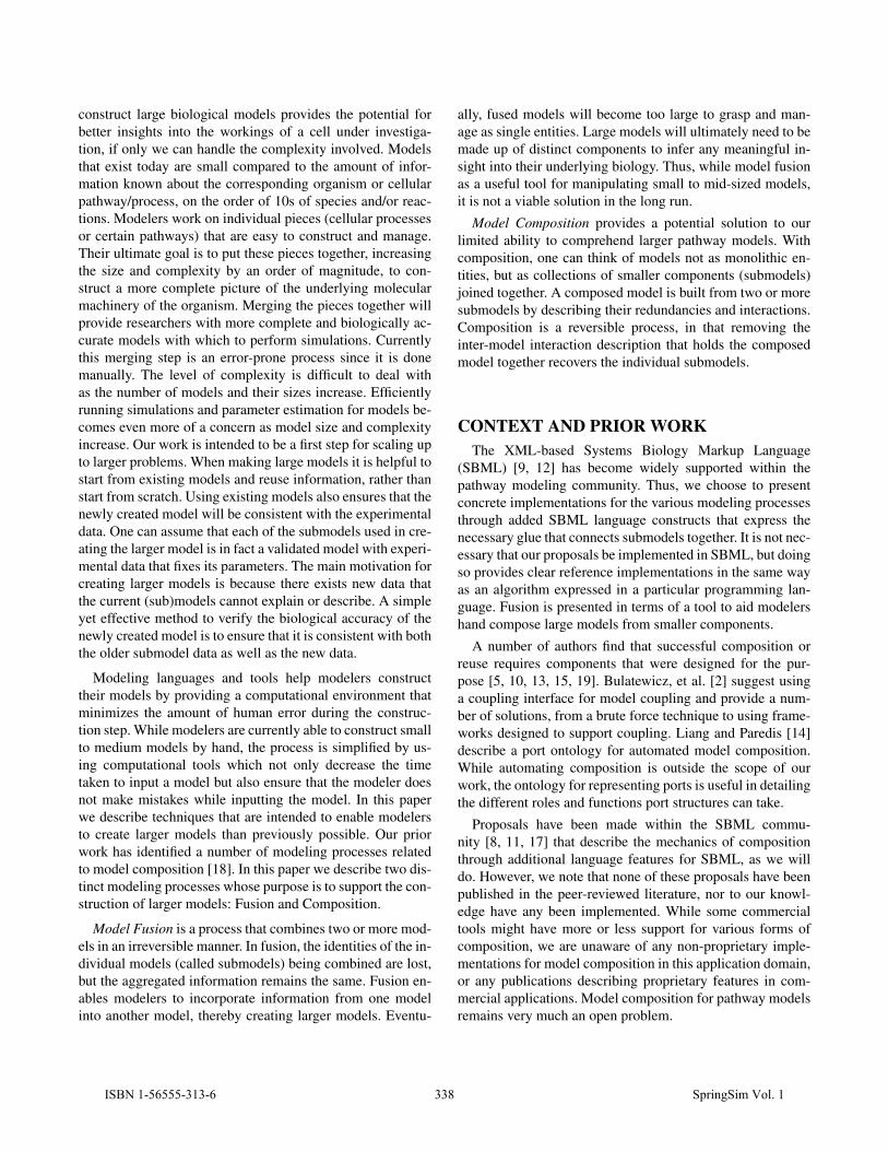
The two sample models in Figure 2 were obtainedfrom [20] and describe how the cell cycle engine is reg-ulated in eukaryotic cells. Model1 describes the effectsof Cdh1/APC, Cdc20/APC and cyclin-Cdk on each other.Model2 describes the effects of a cyclin-dependent kinase in-hibitor (CKI) on CycB.

Consider the two sample models, Model1 andModel2 which will be fused together to produce model(FusedModel). The modeler does this by producing amapping table for the various SBML component types.During this processing we must avoid dependencies acrosscomponents which might exist as some components are ref-erenced in other components. For examples, we must resolvethe identities of compartments (which represent the bounded

Model 2

cell

CycB

Cdh1i Cdh1

TF TFi

SK

CKI

CKICycB

Model 1

cell

CycB

Cdh1i Cdh1

IEPi

IEP

Cdc20i

Cdc20a

SpeciesCompartmentModel

Key

+

Figure 2. Sample models

space in which species are located) before species, since eachspecies stores a reference to its containing compartment interms of a compartment identifier. Fortunately, the followingordering for the eight SBML component types has no suchconflicting dependencies: (1) Compartments; (2) Species; (3)Function Definitions; (4) Rules; (5) Events; (6) Units; (7)Reactions; and (8) Parameters.

A column in a mapping table represents a model, and eachrow represents an SBML component in that model. Duplicatenames within a model are not allowed. Therefore, a speciesname will only occur once in any particular column. The firstcolumn in the mapping table is reserved for the fused modeland is referred to as FusedModel). The two actions availableto the modeler during fusion are:

1. define two or more SBML components to be equivalent2. remove the link/association between two or more SBML

components (which have previously been incorrectlylinked together) across the different submodels.

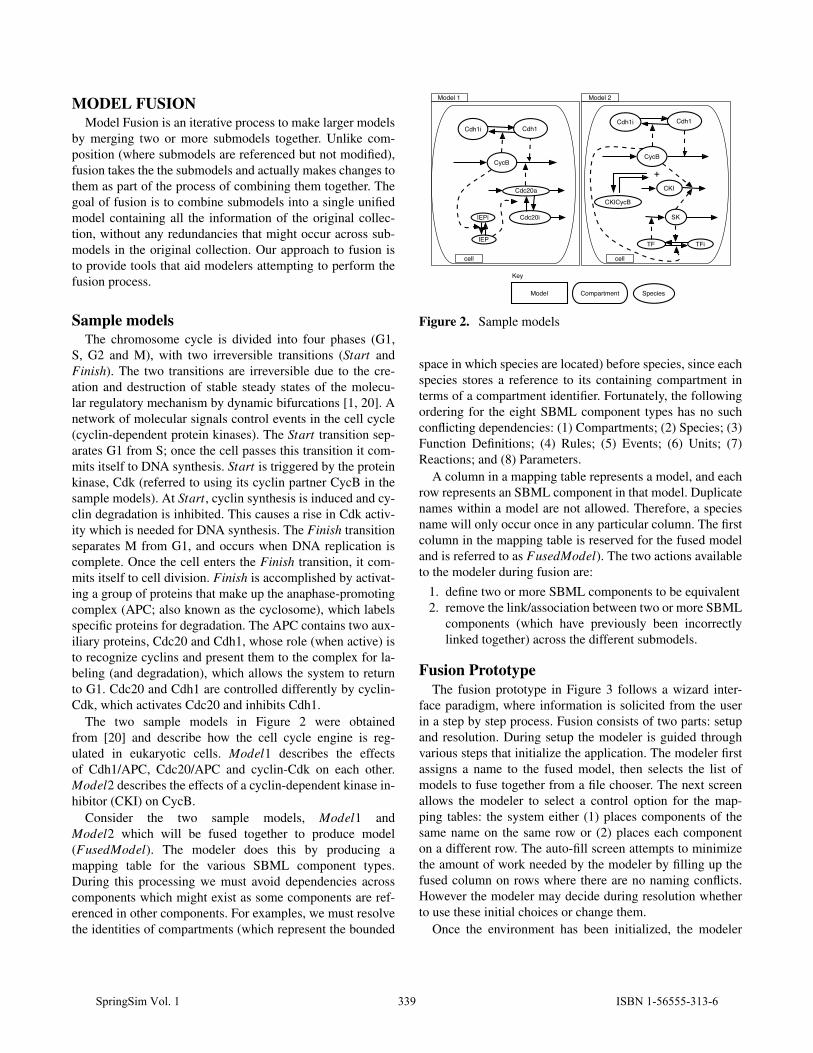
Fusion PrototypeThe fusion prototype in Figure 3 follows a wizard inter-

face paradigm, where information is solicited from the userin a step by step process. Fusion consists of two parts: setupand resolution. During setup the modeler is guided throughvarious steps that initialize the application. The modeler firstassigns a name to the fused model, then selects the list ofmodels to fuse together from a file chooser. The next screenallows the modeler to select a control option for the map-ping tables: the system either (1) places components of thesame name on the same row or (2) places each componenton a different row. The auto-fill screen attempts to minimizethe amount of work needed by the modeler by filling up thefused column on rows where there are no naming conflicts.However the modeler may decide during resolution whetherto use these initial choices or change them.

Once the environment has been initialized, the modeler

SpringSim Vol. 1 339 ISBN 1-56555-313-6

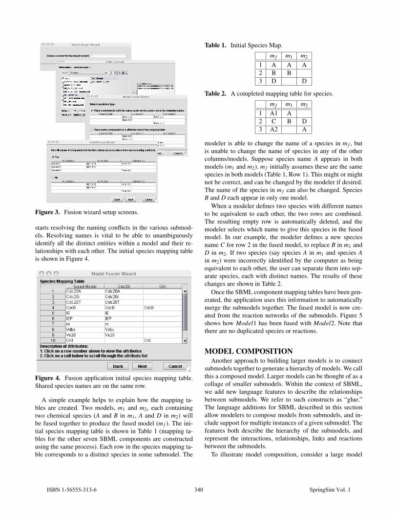
Figure 3. Fusion wizard setup screens.

starts resolving the naming conflicts in the various submod-els. Resolving names is vital to be able to unambiguouslyidentify all the distinct entities within a model and their re-lationships with each other. The initial species mapping tableis shown in Figure 4.

Figure 4. Fusion application initial species mapping table.Shared species names are on the same row.

A simple example helps to explain how the mapping ta-bles are created. Two models, m1 and m2, each containingtwo chemical species (A and B in m1, A and D in m2) willbe fused together to produce the fused model (m f ). The ini-tial species mapping table is shown in Table 1 (mapping ta-bles for the other seven SBML components are constructedusing the same process). Each row in the species mapping ta-ble corresponds to a distinct species in some submodel. The

Table 1. Initial Species Map.

m f m1 m2

1 A A A2 B B3 D D

Table 2. A completed mapping table for species.

m f m1 m2

1 A1 A2 C B D3 A2 A

modeler is able to change the name of a species in m f , butis unable to change the name of species in any of the othercolumns/models. Suppose species name A appears in bothmodels (m1 and m2). m f initially assumes these are the samespecies in both models (Table 1, Row 1). This might or mightnot be correct, and can be changed by the modeler if desired.The name of the species in m f can also be changed. SpeciesB and D each appear in only one model.

When a modeler defines two species with different namesto be equivalent to each other, the two rows are combined.The resulting empty row is automatically deleted, and themodeler selects which name to give this species in the fusedmodel. In our example, the modeler defines a new speciesname C for row 2 in the fused model, to replace B in m1 andD in m2. If two species (say species A in m1 and species Ain m2) were incorrectly identified by the computer as beingequivalent to each other, the user can separate them into sep-arate species, each with distinct names. The results of thesechanges are shown in Table 2.

Once the SBML component mapping tables have been gen-erated, the application uses this information to automaticallymerge the submodels together. The fused model is now cre-ated from the reaction networks of the submodels. Figure 5shows how Model1 has been fused with Model2. Note thatthere are no duplicated species or reactions.

MODEL COMPOSITIONAnother approach to building larger models is to connect

submodels together to generate a hierarchy of models. We callthis a composed model. Larger models can be thought of as acollage of smaller submodels. Within the context of SBML,we add new language features to describe the relationshipsbetween submodels. We refer to such constructs as “glue.”The language additions for SBML described in this sectionallow modelers to compose models from submodels, and in-clude support for multiple instances of a given submodel. Thefeatures both describe the hierarchy of the submodels, andrepresent the interactions, relationships, links and reactionsbetween the submodels.

To illustrate model composition, consider a large model

ISBN 1-56555-313-6 340 SpringSim Vol. 1

CycB

Cdh1 Cdh1

Fused Model

cell

SpeciesCompartmentModel

Key

IEPi

IEP

Cdc20a

Cdc20i

CKI

CKICycB +

SK

TF TFi

Figure 5. The fused model

(called Global), composed of two submodels (A and B).Model A contains the chemical species x and model B con-tains the species y. It is now possible to make a new reactionin Global that represents x → y, by referring to x and y inA and B respectively. Global consists of a model with onlyone reaction. The names of reactants and products for thatreaction refer to the corresponding species in the two sub-models. It should be noted that adding a new reaction (or anynew component) is not performed in the fusion tool, insteadthis action is accomplished in the model building environ-ment used to create the (sub)models.

It turns out that there are significant similarities betweenmodel fusion and model composition, as we discovered dur-ing the process of developing the fusion tool. We had origi-nally conceived of fusion and composition as fairly unrelatedprocesses. However, the fusion process described in the lastsection defines a series of steps taken to merge two or moremodels together. This series of steps is captured by our fu-sion wizard tool, and can be viewed as an “audit trail” used ingenerating the necessary mapping tables. Precisely this sameinformation can be used to describe the set of instructionsneeded to connect/link the submodels for composition. Bothcomposition and fusion should produce the same results, asthe output of both fused and composed models should beidentical during simulation. While fusion combines submod-els together in an irreversible way, composition simply ref-erences submodel components by defining the “glue” thatholds the submodels together. A major difference is that in fu-sion the explicit description of relationships between entitieswithin submodels is lost, while composition keeps a "record"of how models were composed/connected together.

The first step in composition is to assign or select the globalmodel (the root node in the model tree hierarchy), which caneither be one of the submodels or a new model. This requiresextending the fusion wizard’s file chooser functionality to al-

Big

comp1

Little

comp2

Figure 6. Submodel example showing a link between twocompartments

low selecting which of the submodels will become the com-posed model.

A composed model can contain one or more submod-els within its structure. A submodel contains a valid SBMLmodel (an SBML <model> structure), with its own names-pace and can be a composed model. Since there is no re-striction on the number of submodels a model can contain,a <model> structure is enclosed in a <listOfSubmodels>structure. A simple example (Figure 6) shows how model Bigcontains a submodel called Little, and both models containsa single compartment (comp1 and comp2 respectively).

After the list of submodels have been declared in theglobal model, the modeler needs to instantiate the submod-els in order to use/access them using the <Instance> struc-ture. Finally, different components (species, reactions, etc)within either the submodels or the global model are con-nected/accessed using <link> structures.

We adopt a naming convention to enable modelers touniquely identify an SBML component (e.g. species, param-eters, etc) within a model (or submodel). Our format is:

<to object="ObjectIdentifier"><subobject object="SubobjectIdentifier"/>

</to>

We also describe this using the syntax ObjectIdenti-fier.SubobjectIdentifier. This convention makes it possible torefer to SBML components with the same name in differentmodels without having to change their names.

Each <instance> (enclosed in a <listOfInstances> struc-ture) refers to a particular <model>. An <instance> indi-cates that a copy of a submodel is being instantiated withinthe current model. Models can be composed of more thanone instance of a particular submodel. The instance struc-ture uses the XML Linking Language (XLink) [6] to re-fer to submodels, as it is a standard mechanism for link-ing XML elements inside and outside a given SBML docu-ment. XLinks describe links between XML documents. Aninstance of submodel Little (called Submodel_Little) can bemade in model Big in order to use/access submodel Little in

SpringSim Vol. 1 341 ISBN 1-56555-313-6

model Big. The <instance> structure contains attributes id(the unique identifier for the <instance>), the XLink’s type,and the XLink’s hre f (an XPointer string that points to eitheran SBML model document or a model element within thecurrent SBML document) The type attribute takes the valuessimple and extended. A simple link is a link that associatesexactly two resources, one local and one remote. The direc-tion of the link is from the former to the latter and thus isalways an outbound link. An extended link associates an ar-bitrary number of resources. The participating resources mayeach be local or remote. For our example we only need to linktogether two objects (resources) and so the value of the typefield will be simple.

A <link> (enclosed in a <listOfLinks>) links two enti-ties in separate submodels of a composed model. A <link>should be able to link two <species>, <parameters>,<reactions>, or <compartments> to each other. Linkingcomponents in composition can be achieved by using themapping tables created during fusion. Components on thesame row in the mapping table will be linked together. Func-tionality to describe the type of link must be added to thecurrent fusion mapping table to better represent the unidirec-tional relationship between linked components. A <link> iscomposed of two fields, <from> and <to>. The <to> fieldreferences an object (the to object) whose attribute values willbe overridden by the object referenced by the <from> field(the from object). The objects referenced by <from> and<to> fields must be of the same type. Only those attributevalues that have been declared in the from object will be over-ridden in the to object. This is somewhat analogous in C/C++to treating the to object as a pointer, and the from object asits target. However, a to object can have attribute values thatare retained if no overriding attribute value is declared in thefrom object. Note that if we have two components inside a(sub)model we are still able to link subobjects of the compo-nents using our object/suboject naming convention. The fol-lowing example shows how the two compartments in Big andLittle can be linked together (Figure 6).

<model id="Big"><listOfCompartments><compartment id="comp1" volume="1"/>

</listOfCompartments><listOfSubmodels><model id="Little"><listOfCompartments><compartment id="comp2" volume="1"/>

</listOfCompartments></model>

</listOfSubmodels><listOfInstances><instanceid="Submodel_Little"xlink:type="simple"

xlink:href="#xpointer(/sbml/model/listOfSubmodels/model[@id=Little])"/>

</listOfInstances><listOfLinks><link><from object="comp1"/><to object="Submodel_Little"><subobject object="comp2"/>

</to></link>

</listOfLinks></model>

The above example shows an href attribute where the sub-model Little occurs within the same SBML document. If thesubmodel Little occurred in another SBML document namedtemp.sbml in the current directory, the href attribute of the<instance> structure would have temp.sbml prepended to it.

The <link> structure contains a merge attribute, whosevalue can be either true (indicating a merge link) or false(indicating a replacement link). To see the difference, con-sider models R and T which each contain a chemical speciescalled S1 with different attributes. S1 in Model R has attributeA = 1.0. S1 in Model T has attributes A = 2.0 and B = 3.0.Linking S1 in R to S1 in T with a merge link uses S1’s at-tributes from T .S1 that have not been declared in R.S1. Thus,the result is that S1 has attributes A = 1.0 and B = 3.0 sinceit keeps its old value for A and gains the definition for B. IfS1 in R is linked to S1 in T using a replacement link (i.e., themerge attribute is false), then only R.S1’s attributes are used.Thus, the result will be that S1 will have attribute A = 1.0.Specifying the type of link for composition requires includ-ing an additional field to the mapping table to specify themerge/replacement attribute.

The <link> structure can link certain combinations ofdiffering SBML component types to each other, such asspecies ↔ parameters and rules ↔ species/parameters. Alink can take a <species> structure as the from object anda <parameter> structure as the to object, and vice versa.An example of this type of link is found when composingthe two sample models sharing a degradation reaction CycB(CycB →). In Model1 this reaction contains the modifierCdc20a, but in Model2, this species does not exist so thereaction instead contains the parameter A. In the composedmodel the species Cdc20a from Model1 will be linked to theparameter A in Model2. The reason for this link is becausewhen Model2 was created, knowledge about Cdc20a was notknown so the modeler used the entity (parameter) A in theirmodel instead. When Model1 was created the modeler hadknowledge about the effects of Cdc20a on CycB degradation.With this additional knowledge it is now desirable to replaceA with Cdc20a when composing (or fusing) the two modelstogether.

ISBN 1-56555-313-6 342 SpringSim Vol. 1

FUTURE PLANSWe will investigate two additional modeling processes

whose purpose is to support the construction of larger models.Model Aggregation is a restricted form of composition. A col-lection of model elements is represented as a single entity (a“module”). A module contains a list of input and output portsthat link to internal species and parameters. These ports de-fine the module’s interface, which provides restricted accessto the components in the module. The process of aggregation(connecting modules via their interfaces) allows modelers tocreate larger models in a controlled manner. It is possible thatmodel aggregation will prove to be more intuitive to modelerswho are constructing large models from scratch with compo-nents designed to be aggregated, rather than composing exist-ing models that have incompatibilities.

Model Flattening converts a composed or aggregatedmodel with some hierarchy or connections to one withoutsuch connections. The result is equivalent to fusing the sub-models. However, the relationship information provided bythe composition and/or aggregation process should be suffi-cient to allow the flattening to take place without human in-tervention (such intervention is needed in the fusion processsince this information is unknown to the fusion tool). The re-lationships used to describe the interaction between the mod-els and submodels are lost, as the composed or aggregatedmodel is converted into a single large (fused) model. Flat-tening a model allows us to use existing tools that have nosupport for composition or aggregation.

REFERENCES[1] M.T. Borisuk and J.J. Tyson. Bifurcation analysis of a

model of mitotic control in frog eggs. Journal of Theo-retical Biology, 195(1):69–85, 1998.

[2] T. Bulatewicz, J. Cuny, and M. Warman. The poten-tial coupling interface: Metadata for model coupling. InProceedings of the 2004 Winter Simulation Conference,pages 183–190, 2004.

[3] K.C. Chen, L. Calzone, A. Csikasz-Nagy, F.R. Cross,B. Novak, and J.J. Tyson. Integrative analysis of cellcycle control in budding yeast. Mol Biol Cell, 15:3841–3862, 2004.

[4] DARPA. Darpa biospice website. Available atcommunity.biospice.org, 2005.

[5] P.K. Davis and R.H. Anderson. Improving the compos-ability of DoD models and simulations. Journal of De-fense Modeling and Simulation, 1(1):5–17, 2004.

[6] S. DeRose, E. Maler, and D. Orchard. Xml linking lan-guage (xlink) version 1.0 w3c recommendation. Avail-able at www.w3.org/TR/xlink, 2001.

[7] DOE. Us department of energy genomes to life website.Available at doegenomestolife.org/, 2005.

[8] A. Finney. Systems biology markup language (sbml)level 3 proposal: Model composition features. Avail-able at www.sbml.org/forums/index.php?t=tree&goto=171&rid=0, 2003.

[9] A. Finney, M. Hucka, and H. Bolouri. Systems biol-ogy markup language (sbml) level 2: Structures andfacilities for model definitions. Available at sbml.org/specifications/sbml-level-2/version-1/html/sbml-level-2.html, 2002.

[10] D. Garlan, R. Allen, and J. Ockerbloom. Architecturalmismatch or why it’s hard to build systems out of ex-isting parts. In International Conference on SoftwareEngineering, pages 179–185, 1995.

[11] M. Ginkel. Modular sbml proposal for an extension ofsbml towards level 2. In Proceedings of 5th Forum onSoftware Platforms for Systems Biology, 2003.

[12] M. Hucka, A. Finney, H.M. Sauro, and 40 additional au-thors. The systems biology markup language (SBML):a medium for representation and exchange of biochem-ical network models. Bioinformatics, 19(4):524–531,2003.

[13] S. Kasputis and H.C. Ng. Model composability: for-mulating a research thrust: composable simulations. InProceedings of the 2000 Winter Simulation Conference,pages 1577–1584, 2000.

[14] V.C. Liang and C.J.J. Paredis. Foundations of multi-paradigm modeling and simulation: a port ontology forautomated model composition. In Proceedings of the2003 Winter Simulation Conference, pages 613–622,2003.

[15] R.J. Malak and C.J.J. Paredis. Foundations of validat-ing reusable behavioral models in engineering designproblems. In Proceedings of the 2004 Winter Simula-tion Conference, pages 420–428, 2004.

[16] G. Marlovits, C.J. Tyson, B. Novak, and J.J. Tyson.Modeling M-phase control in Xenopus oocyte extracts:the surveillance mechanism for unreplicated DNA. Bio-physical Chemistry, 72:169–184, 1998.

[17] D. Schroder and J. Weimar. Modularization ofsbml. Available at www.sbml.org/workshops/ninth/VortragSBMLForum.pdf, 2003.

[18] C.A. Shaffer, R. Randhawa, and J.J. Tyson. The role ofcomposition and aggregation in modeling macromolec-ular regulatory networks. In Proceedings of the 2006Winter Simulation Conference, Dec. 2006.

SpringSim Vol. 1 343 ISBN 1-56555-313-6

[19] M. Spiegel, P.F. Reynolds, and D.C. Brogan. A casestudy of model context for simulation composabilityand reusability. In Proceedings of the 2005 Winter Sim-ulation Conference, pages 437–444, 2005.

[20] J.J. Tyson and B. Novak. Regulation of the eukary-otic cell cycle: Molecular antagonism, hysteresis, andirreversible transitions. Journal of Theoretical Biology,210:249–263, 2001.

AUTHOR BIOGRAPHIESRANJIT RANDHAWA is a PhD candidate in the Depart-ment of Computer Science at Virginia Tech. He received BSdegrees in Computer Science and Genetic Biology from Pur-due University, and an MS degree in Computer Science fromVirginia Tech. His research interests include software design,systems biology, synthetic biology, computational biology,bioinformatics and modeling and simulation.

CLIFFORD A. SHAFFER is an associate professor in theDepartment of Computer Science at Virginia Tech since1987. He received his PhD from University of Maryland in1986. His current research interests include problem solvingenvironments, bioinformatics, component architectures, visu-alization, algorithm design and analysis, and data structures.His Web address is www.cs.vt.edu/shaffer.

JOHN J. TYSON is University Distinguished Professor ofBiological Sciences at Virginia Tech. He received his PhDin chemical physics from the University of Chicago in 1973and has been specializing in theoretical cell biology since thattime. His current interests revolve around the gene-protein in-teraction networks that regulate features of cell physiologysuch as cell division, circadian rhythms, intracellular signal-ing networks, and programmed cell death.

ISBN 1-56555-313-6 344 SpringSim Vol. 1