AD-A15i 512 FURTHER DEVELOPMENTS OF THE MOMENTUM INTEGRAL METHOD i/iFOR BOUNDARY LAVERS(U) SCIENCE AiPPLICATIONS INCANNAPOLIS ND C H VON KERCZEK ET AL- 16 MAY 84

UNCLASSIFIED S I-84/34 N8 8i24-B--0 F/28/4 NL

.. lul ,__. 11112-

111.

1.25111112.L

LL

MICROCOPY RESOLUTION TEST CHART

NATIONAL BUREAU OF STANDARDS-1963 A

*'-- 1. FURTHER DEVELOPMENTS OFTHE MOMENTUM INTEGRAL METHOD FOR

SHIP BOUNDARY LAYERS

SAI-84/ 3046

* z..t

-~ 3

**1 3~

4 J. -

SCEC .PUATOS INC.

- 1203

FURTHER DEVELOPMENTS OF

THE MOMENTUM INTEGRAL METHOD FOR

SHIP BOUNDARY LAYERS

SAI-84/3046

Science Aplications International Corp tion134 Holiday Court, Suite 318, Annapolis, Maryland 21401, (301) 266-0991 ELL C .

MAR 2 0 1985

This docuent has been approved

for pblic release and sale; itsdi trib utio nis un im ited ,

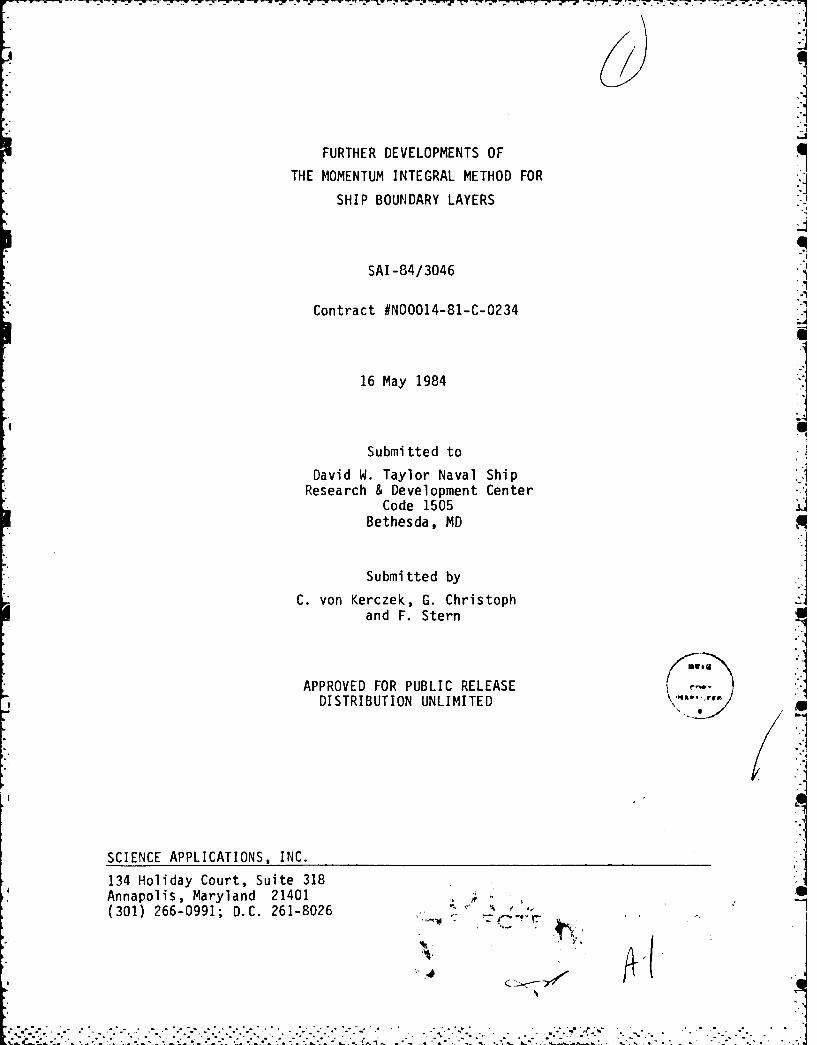
FURTHER DEVELOPMENTS OF

THE MOMENTUM INTEGRAL METHOD FOR

SHIP BOUNDARY LAYERS

SAI-84/3046

Contract #N00014-81-C-0234

16 May 1984

Submitted to

David W. Taylor Naval ShipResearch & Development Center

Code 1505Bethesda, MD

Submitted by

C. von Kerczek, G. Christophand F. Stern

APPROVED FOR PUBLIC RELEASEDISTRIBUTION UNLIMITED " ,rip

SCIENCE APPLICATIONS, INC.

134 Holiday Court, Suite 318Annapolis, Maryland 21401(301) 266-0991; D.C. 261-8026 .

4

UNCLASSI FIED

SECURITY CLASSIFICATION OF THIS PAGE (When Dore Entered)

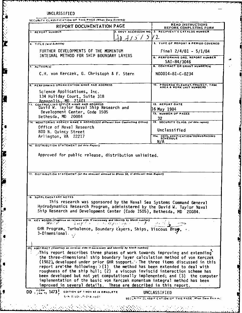
REPORT DOCUMENTATION PAGE READ INSTRUCTIONSCESSIO NOA BEFORE COMPLETING FORM

t. REPORT NUMBER 2. GOVT ACCESSION NO. 3. RECIPIENT'S CATALOG NUMBER

4. TITLE (endSubtItle) S. TYPE OF REPORT & PERIOD COVERED

FURTHER DEVELOPMENTS OF THE MOMENTUM Final 2/4/81 - 5/1/84INTEGRAL METHOD FOR SHIP BOUNDARY LAYERS 6. PERFORMING ORG. REPORT NUMBER

SAI-84/30467. AUTHOR(&) I. CONTRACT OR GRANT NUMBER(s)

C.H. von Kerczek, G. Christoph & F. Stern N00014-81-C-0234

*9. PERFORMING ORGANIZATION NAME AND ADDRESS .10 PROGRAM ELEMENT. PROJECT. TASKAREA & WORK UNIT NUMBERS

Science Applications, Inc.134 Holiday Court, Suite 318Annapnlis, Mn 71401

I. CONTROLLING OFFICE NAME AND ADDRESS 12. REPORT DATE

David W. Taylor Naval Ship Research and 16 May 1984Development Center, Code 1505 13. NUMBER OF PAGES

Bethesda, MD 20084 3214. MONITORING AGENCY NAME & AOORESS(l different from Controlling Office) IS. SECURITY CLASS. (of this report)

Office of Naval Research800 N. Quincy Street UnclassifiedArlington, VA 22217 IS. O ASSIFICATION/OWNGRADINGSCHEDULE

N/A16. DISTRIBUTION STATEMENT (of thIs Report)

Approved for public release, distribution unlimited.

17. DISTRIBUTION STATEMENT (of the abstract entered In Block 20, If different from Report)

IW. SUPPLEMENTARY NOTES

This research was sponsored by the Naval Sea Systems Command GeneralHydrodynamics Research Program, administered by the David W. Taylor NavalShip Research and Development Center (Code 1505), Bethesda, MD 20084.

19. KEY WORS (Coeinue on reveree side It necessary id Identify by block number). ':. -. t, . ,

GHR Program, Turbulence, Boundary tayers, Ships, Viscous Ura9,3-Dimensional

6l

20j ABSTRACT (Continue on re8ere sde If neceeoty and Identify by block number)

,This report describes three phases of work towards improving and extending"the three-dimensional ship boundary layer calculation method of von Kerczek(1982).developed under prior GHR support.-, The three items discussed in thisreport arelthe following: ) (1) the method has been extended to deal withroughness of the ship hull; (2) a viscous inviscid interaction scheme hasbeen developed but not yet computationally implemented; and (3) the computerimplementation of the basic von Kerczek momentum integral method has beenimproved in several details. These are described in this report.

D D I '" 3 1473 EoITIOd OF I NOV 65 IS OBSOLETE UNCLASSIFIEDS I N ) ; %) 2 - - c - 0 1 4 - C I S E C ', R Z 1 _ " S S cI C A T I O N O

rT 4 I S P 4 G E % n D e oe 9 i' . e "

TABLE OF CONTENTS

1.0 INTRODUCTION. .. ..... ....... ...... ..... 1-1

2.0 A GENERAL PROCEDURE FOR INCLUDING ROUGHNESS EFFECTS IN THEINTEGRAL BOUNDARY LAYER EQUATIONS. .. .. ....... .... 2-1

2.1 Introduction. .. .. ....... ........ ..... 2-12.2 Solution Procedure for 2-D Boundary Layers .. .. .. . .. 2-22.3 Extension to 3-D. .. .. ....... ....... ... 2-52.4 Computational Results. .. ..... ........ ... 2-6

3.0 VISCOUS-INVISCID INTERACTIONS .. .. ..... ....... .. 3-1

3.1 Introduction. .. .. ....... ...... ....... 3-13.2 Axisymmetric Viscous-Inviscid Interactions. .. .. .... 3-23.3 Three-Dimensional Viscous-Inviscid Interactions .. .. .. 3-9

4.0 COMPUTATIONAL IMPROVEMENTS TO THE BASIC MOMENTUMOINTEGRAL METHOD .. .. .... ....... ........ .. 4-1

Appendix Unsuccessful Method for Calculating Viscous-InviscidInteractions at a Stern-...............A-1

*References. .. ..... ....... ........ ....... .. R-1

ABSTRACT

This report describes three phases of work towards improving and

extending the three-dimensional ship boundary layer calculation method of

von Kerczek (1982) developed under prior GHR support. The three items dis-

- cussed in this report are the following: (1) the method has been extended

• .to deal with roughness of the ship hull; (2) a viscous inviscid interac-

tion scheme has been developed but not yet computationally implemented; and

(3) the computer implementation of the basic von Kerczek momentum integral

method has been improved in several details. These are described in this

report.

03

0

0

ii

*%. . -• . . :. *.'.. * *- * . . . . * . . . 7 . . . 1

01

1.0 INTRODUCTION

Under prior GHR support von Kerczek (1982) (henceforth referred to

as K) developed a momentum integral ship boundary layer calculation method

which seems to be a promising, relatively simple and useful way of estimating

the viscous flow and some of its consequences. This method is capable of

dealing with reversed cross-flow boundary layer velocity profiles and thus

can be made more acucrate than prior momentum integral methods for ships

(see von Kerczek and Langan, 1979).

The method of K has already been put to use to calculate the

total drag of a destroyer hull (von Kerczek, et al., 1983) and as an aid in

determining appendage drag (Stern and von Kerczek, 1983). These applica-

* -tions are still tentative and require further verification and refinement.

However, the results are encouraging and also have pointed the way towards

some of the more important weaknesses of the method of K.

Under further GHR support, for which this report is presented,

three items have been considered to improve the K method. These are the

following:

(1) The method of K has been extended to deal with roughness of the

ship hull.

(2) A method for viscous-inviscid interaction has been developed,

but not yet computationally implemented.

(3) The computer implementation of the basic method of K has beenimproved in several details making it more reliable and accurate.

This report details each of these efforts.

0

2.0 A GENERAL PROCEDURE FOR INCLUDING ROUGHNESS EFFECTS IN THE

INTEGRAL BOUNDARY LAYER EQUATIONS

2.1 Introduction

Most roughness analyses are based on Nikuradse's sand-grain

experiments and fitting of the law-of-the-wall velocity profiles to experi-

mental data. Several correlations have been proposed to relate real

roughness heights, spacings and geometries to an equivalent sand-grain

height so that Nikuradse's data can be used. Examples of such correlations

can be found in Betterman (1966), Simpson (1973) and Dirling (1973). These

correlations are not very accurate for closely spaced roughness elements

such as those found on a ship's surface. The correlations in these refer-

ences are biased toward data for roughness elements with large spacings.

More meaningful methods that account for actual roughness effects

are those employed by Christoph and Pletcher (1983), Finson and Clarke (1980)

and Lin and Bywater (1982). These techniques calculate the form-drag con-

tributions of individual elements. Roughness elements are assumed to occupy

no physical space. The governing boundary layer equations are cast in a

form to account for the blockage effects of the roughness elements. Terms

that act in the streamwise direction are multiplied by the factor [1-D(y)/I,

where D(y) is the element width at height y and Z is the average center-to-

center spacing. Terms that act in the direction normal to the streamwise

direction are multiplied by [1-irD2 (y)/(4X2 )]. The effect of roughness in

the momentum equations is described by a sink term and represents form drag.

To date, the form drag approach has been taken only with a finite-

difference solution of the boundary layer equations. In order to apply this

method directly to a 3-dimensional integral technique such as that of K, a

skin friction correlation that explicitly accounts for roughness height,spacing and geometry has to be specified. This is not yet possible; instead,

the following approach is taken here.

2-1

, '. ,- , . , - . . . '- .' ,' .. ,.. -. .. .," ,. ' . - -,'. -.. ' - - 7

A

Based on results of numerous computer runs with a variety of rough-

ness shapes and spacings, Finson (1982) suggested a correlation relating

equivalent sand-grain height to roughness height, spacing and geometry.

This correlation was shown by Finson to be accurate for closely packed ele-

ments. Using calculated equivalent sand-grain heights, a method was devel-

oped in this study to calculate skin friction, boundary layer thickness and

velocity profiles based on classical sand-grain roughness relations. The

details are described below.

2.2 Solution Procedure for 2-D Boundary Layers

It is desirable to include roughness in the full 3-D boundary

layer equations using Head's entrainment technique as implemented by K. To

begin the development, the roughness methodology is most easily discussed -

in the framework of a 2-D flow. Extension to 3-D and its implementation

are discussed later. The 2-D momentum integral equation is

dO cf 2+H dU (2-1)

and the boundary layer entrainment equation is

-F(G) _4q (2-2)ds Uds

where

q = Ge, H = 6/0. (2-3)

The skin friction coefficient cf, Head's shape factor G, and the rate of

entrainment function F(G) are modelled in the same way as in K. In the

present study it is assumed that roughness effects are accounted for simply

by including roughness in the skin friction model. The momentum thickness

0 and the shape factor H are affected by roughness through integration of

equations (2-1) and (2-2). The process of entrainment is mainly controlled

by the velocity defect in the outer part of the boundary layer and therefore

the entrainment, as used in K, should not be affected by roughness. The

2-2

I

. - .-. . .

magnitude of the entrainment variables (G and F) will change, however, due

to their dependence on H.

Roughness effects are modelled in cf through the classical velocity

shift, that is,

u u - AB (2-4)L ur = s

wherei + 1 y+

us = n K ny + CONSTANT, K 0.41

(2-5)

AB ln k+ - 3K esand

+ yu/v, k + k u*/ves es

(2-6)u = u/u*, U* = (Tw/P)

The subscripts s and r refer to smooth and rough conditions, respectively.

Since

+ 112

Uedge = (2/cf)1 , (2-7)

the rough wall skin friction coefficient cfr is related to the smooth wall

skin friction coefficient Cfs by

(2/cfr)1/2 = (2/cf s )I/2 - AB. (2-8)

If c and k are known, then Cfr is easily solved from equation (2-8). Thisfs es f

is done by rewriting equation (2-8) as

1/2 1 1/2= 1/2 1(2/c r) n (2/cfr) (2/cf s ) - In Re 4 3

kes (2-9)

(Rekes =Ue kes/V)

2-3

.. .. ,-- . . " .- - *',- ,. ". . - *.- ,. -.- . 2. . ...- . .. .

and using an iteration scheme, e.g., Newton-Raphson, to solve for cfr. The

method used for determining kes is discussed next.

In the form drag analysis outlined in the introduction, the wall

shear is given by

k 2Cfr =Cf + c c0 f(y) dy (2-10)

where1 - D(y)/Z

f(y) = (2-11)1 - TrD2 (y)/(49,2)

and co is a form drag coefficient. Taking u = UR = constant, cD = constant,

and evaluating f(y) at y = k/2, equation (2-10) becomesCfr = Cfs + (2-12

Ue cD f(k/2)/X k. (2-12)

The parameter

-1

X = projected frontal area of the elements per (2-13)unit surface area.

Based on numerous calculations for cD = 0.6, Cfs at Re = 10 , and k/e = 1,

Finson (1982) recommends the correlation

UR= 0.247 + 0.234 log o Xk (2-14)

e

So for the above conditions equation (2-12) becomes

Cfr = Cfs (Re= 10 s) + 0.6(0.247+ 0.234 og loAk) f(k/ 2 )/Xk. (2-15)

A simple relation can be obtained for the equivalent sand-grain height, kes,

if cfs is approximated by

2-4

(2/cfs 2 -k n Re8 + C (flow geometry, pressure gradient). (2-16)

Equation (2-9) can be rewritten as

(2/c -) 1 /8)n(k + C + 3. (2-17)

fs K 2Cfr) es/(217

A general expression for kes is obtained by using Finson's correlation (= k)

and rearranging equation (2-17) to

kees exp [K(C+3- (2/c + n(2/C 2. (2-18)

k (lfr) K~ n fr~j

For C equal to its flat plate value of 5.5, c + 3 = 8.5. This represents

flat plate flow in a fully rough regime.

2.3 Extension to 3-D

The approach taken for 3-D flows is a direct extension of the 2-D

roughness analysis just discussed. The streamwise skin friction coefficient,

cfl, that occurs in the streamwise momentum equation is replaced by the rough

wall skin friction model outlined above. Rough wall values of 611, H and 821

(see K for notation) are then generated by solving equations (2-6) - (2-8) of

K. The cross flow skin friction coefficient, cf2 , is computed from

cf2 = Cfl tanO (2-19)

where tan6 is calculated from equation (5) of K. It should be noted that

the rough wall skin friction calculation by equation (2-9) requires knowl-

edge of the smooth wall skin friction. Therefore, the smooth and rough

wall flows need to be calculated in parallel.

In order to obtain the crossflow boundary layer thickness, 621

and 612' it is necessary to know how roughness affects the streamwise andcrossflow velocity profiles. Roughness effects were included in the stream-

wise velocity profile as follows. Equation (2-4) is written as

2-5

q

. ... . . ..-

U /u u /u - n (k u*/v) + 3 (2-20)r sUs K es r

This is rearranged as

ur/U = U/U (c/c)2 + (c/2)' [- n((2/c) ) (2-21)r e s e fr fs +(fr Kfr

- 1 Kn (kes u/v) + 3]K e

where Us/Ue is a smooth wall boundary layer velocity profile. For the results

of this study, the profile of Kool (see K) was used. The crossflow profile

is then calculated by using equation (2-21) as the streamwise profile in

equation (3) of K. It is also necessary to know the rough wall nominal

boundary layer thickness. It is calculated from the relation

= 11 (G + H) (?-22)

where 011, G and H are rough wall values.

2.4 Computational Results

The roughness approach described above was validated by comparison

to the 2-D flow roughness data of Schlichting (1937) and Healzer, Moffat and

Kays (1974). First, comparisons were made to Schlichting's channel flow data

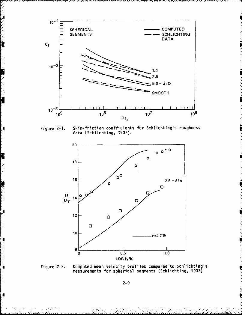
where various arrangements of roughness elements were used. Figure 2-1 gives

skin friction coefficient data versus distance Reynolds number (as presented

by Finson and Clarke (1980)) for spherical segments with element spacings

of L/D(o) = 1, 2.5 and 5. The present predictions are in excellent agree-

ment with the data except at low Reynolds numbers and correctly predict the

effect of element spacing. Figure 2-2 compares the rough wall velocity pro-

file, equation (2-21), with profile data taken by Schlichting. the compari-

son of the profiles is for the top of the roughness elements out towards

the edge of the boundary layer. It appears that equation (2-21) overpre-

dicts the momentum deficit close to the wall. This overprediction is due

2-6

: : ";' " ' . . " , - " ,." " . . ." : . , . ,: . -: , . . ./

to the presence of the roughness elements.

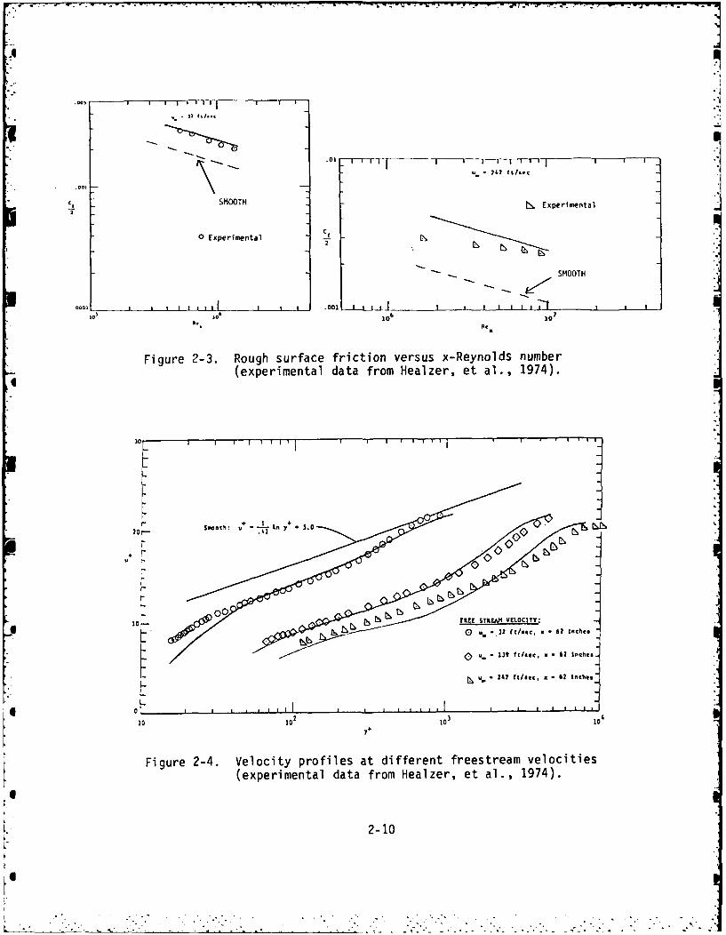
The incompressible flow experiments of Healzer, et al. (1974) pro-

vide data on skin friction, heat transfer and velocity profiles for rough

surfaces with and without blowing. The rough surface consisted of a regular

array of tightly packed (L/D(o) = 1) hemispherical elements, each 0.05 inches

in diameter. Tests were run at freestream velocities of 32, 139 and 242

ft/sec. Comparison of the skin friction coefficients are shown in Figure

2-3 for freestream velocities of 32 and 242 ft/sec. Even though the values

of the calculated skin friction coefficient overpredicts the experimental

values, the equivalent sand-grain height calculated from equation (2-18) is

in excellement agreement with the value used by Healzer, et al. These values

are 0.032 inches for the predictions as compared to 0.031 inches suggested

by Healzer, et al. based on Schlichting's data. Since the roughness elements

in the Healzer, et al. experiments were touching each other, it was necessary

to define a new y origin. The y location at D(y) = 0.99 D(o) was arbitrarily

chosen as the reference level. Velocity profile predictions and data are

compared in Figure 2-4. Since predicted skin friction coefficients were

high, predicted velocity profiles were normalized by the experimental edge

values of u+. Again, it appears that predicted velocities are too low very

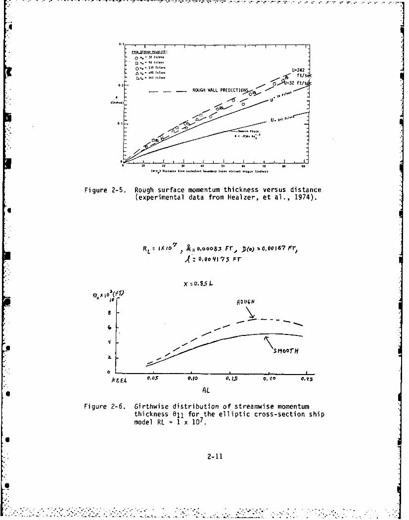
near the wall. Comparisons to the rough-wall predictions for momentum

thickness are shown in Figure 2-5. The increase in the values of 0 due to

roughness and the lesser sensitivity to freestream velocity are correctly

predicted.

No rough-wall skin friction data seems to exist for 3-D flows.

Therefore, only hypothetical cases could be considered. Sample cases were

run for a Reynolds number representative of a full-scale ship (RL = 2x 109)

and a Reynolds number representative of a wind tunnel model (RL = 1x 107).

The sample ship was the same elliptic cross-section body a- the sample case

of K. A reference smooth wall case was run at each Reynolds number along

with roughnesses defined by an equivalent sand-grain height or roughness

element height, base diameter and center-to-center spacing. For the

2-7

".' ? . , - '.. . '.- - " -, -? - -? . -? --',"., - .-.. . -i.-. -- ' : . ,. , ,- . ,.-. - . , L

roughness calculations it is also necessary to input a characteristic length

(ship length). In the present form of the computer code only spherical

segment roughness elements are considered. For the results presented here

k = 0.00083 ft., D(0) =0.00167 ft., and Z, = 0.004175 ft. The ship lengths

used were 1000 feet for the full scale model and 10 feet for the wind tun-

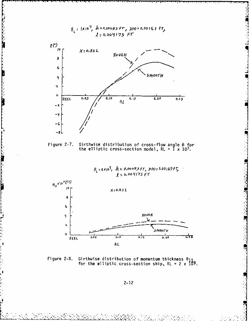
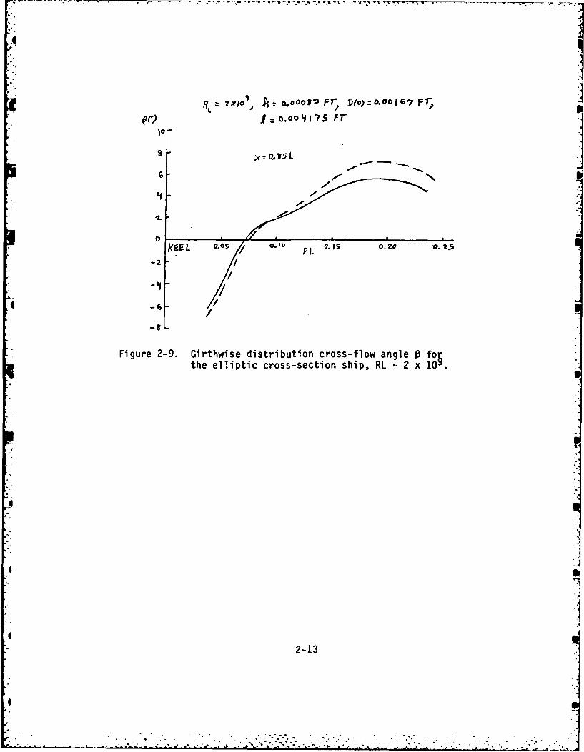
nel model. Plots of the streamwise momentum thickness and the crossflow

angle versus arc length along the girth at X/L = 0.84 are given in Figures

-2-6 and 2-7 for RL = 1x X 0 and in Figures 2-8 and 2-9 for RL =2 x 109.

As expected the momentum thickness increases with roughness. However, as

shown in Figures 2-6 and 2-8, this increase is significantly less near the

keel. This phenomenon is noticeable as one approaches the stern. Roughness

*was predicted to enhance the crossflow angle a (see Figures 2-7 and 2-9).

* This is especially true as the waterline is approached. Intuitively, this 2result was not expected. It was felt that surface roughness would tend to

wash out three-dimensional effects, not enhance them. Measurements, or

perhaps more exact calculations, are needed to more precisely define sur-

face roughness effects in three-dimensional flows.

These 3-D calculations only serve the purpose of indicating that

this roughness theory has been implemented and debugged in the computer pro-

grams of von Kerczek (1983) corresponding to the 3-D boundary layer theory of eK. It would be very valuable to do some numerical experiments with this pro-

gram. One set of tests that would be valuable is a calculation of the

drag increment AC0 obtained by calculating the skin friction drag for a

*smooth and a rough hull. The form drag of Granville (1974), which only

depends on C0 and the potential flow, can be used to complete the determina-

K.tion of AC 0. Although no detailed 3-D roughness boundary layer measurements

seem to be available, there probably is some data (possibly for full scale

4 ships) for which AC0 has been determined. For example, surely trials on a

r. new ship and then later when the ship has aged have been performed. A thor-

K ough literature search for such cases would be highly desirable.

2-8

• . . . . - - C r. - . - . ; . Vo - - C. ° - . . t' _ rW W 4 W . ." .. v W U .. , .'- '- C:. , . °

10-1

SPHERICAL COMPUTEDSEGMENTS SCHLICHTING

DATACf

10-2.-

Cfio~ 2 *1.0

2.5- ' . 5.o 0 ID

SMOOTH

10I f31tl I I IIIIII I 11I 11I1

105 106 107 108

Rex

4 Figure 2-1. Skin-friction coefficients for Schlichting's roughnessdata (Schlichting, 1937).

20

18 005.0

0

0 0

16 - ° o(

160 2.5 = /

U0

14 2

10____PREDICTED

8 I I0 0.5 1.0

LOG (y/k)

Figure 2-2. Computed mean velocity profiles compared to Schlichting'smeasurements for spherical segments (Schlichting, 1937)

2-9

- - ' , . z .. -- . .. _~ . W. ' .2 " '" "" "" " . x . . . ." " ,t". . " " " ' . . '

.01 ------11 .

SMOOTH S Experimentalj

0 Experimental CfTyr

SMOOTH

.0001 1 1 t I III .001 [ k i ll7

0. 10 16 7010 20

Fi gure 2-3. Rough surface friction versus x-Reynolds number(experimental data from Healzer, et al., 1974).

20-

U.* 242 fL/sec. x 6 2 Inches-

1010 2 10 31

Figure 2-4. Velocity profiles at different freestream velocities(experimental data from Healzer, et al., 1974).

2-10

0.0 II

0 9 W ii*

~. *,o 00 ii.. ~ft/s_- 202 lii.. -g5 =32ft

.2- - - ROUGH WALL RDCI>9 wo

0 U. "

05

0 0 20 20 40 20 60 70 00 90

Figure 2-5. Rough surface momentum thickness versus distance(experimental data from Healzer, et al., 1974).

.,:O1/757

R ~ Ix .S5L

II RDUGH

k'-EL 0.0s 0.10 0. J.5 0.,40

Figure 2-6. Girthwise distribution of streaniwise momentumthickness 61 for the elliptic cross-section shipmodel RL =1 x 107.

2-11

o.:,ooVI75 F7

S10~t X:.85 0

-L

10L X=~50.85 0L 40 01

Figure 2-7. Girthwise distribution of moss-flow ahcnessfofthe elliptic cross-section odel, RL 2 1 x 9

22.

44

ILI

L L 0.05; . 5;

th ellip i L ]rs-eto hp L 2x1

2-

4A

-l /'t /

/-8

Figure 2-9. Girthwise distribution cross-flow angle B fo~the elliptic cross-section ship, RL = 2 x 10 .

2-13

Ii

3.0 VISCOUS-INVISCID INTERACTIONS

3.1 Introduction

It has been well established now that the stern boundary layer and

near wake cannot be handled by classical boundary layer theory alone (see

Larson, 1981 and Patel, 1983). The stern boundary layer is fairly thick and 4

causes a considerable disturbance to the bare body potential flow. There

are two currently popular ways to deal with the stern flow. One way is by

using boundary layer theory with viscous-inviscid interactions and the other

way is -by abandoning the boundary layer equations in favor of the "Parabol-

ized Navier-Stokes" (PNS) equations (see, for example, Hogan, 1983). The

latter method is very complex and relies more heavily on large computers

and computing budgets. In keeping with the overall simplicity and practi-

cality of the momentum integral method it is desirable to develop a-rela-

tively simple way to do viscous-inviscid interaction calculations. It is

not expected that such a method will be as accurate as PNS calculations (if

they ever do become fully developed) or even viscous-inviscid interaction

methods based on finite differenced full higher order boundary layer equa-

tions (if these can ever be made to work for ship sterns), but at least a

small improvement at the stern of the basically simple and practical momen-

tum integral method seems worthwhile.

A considerable effort has been expanded to develop a momentum

integral-based method of viscous-inviscid interaction. This effort was at

first unsuccessful. (For completeness, a brief outline of this effort is

given in the appendix.) Unfortunately, the limited budget of this contract

did not allow completion of a new method which has been developed and is

believed to hold considerable promise. This new method of viscous-inviscid

interaction is detailed below. The method is based on the boundary layer

momentum integral equations and slender body potential flow theory.

3-1

'" '.'T ' " .' L ". . .' -' . ..- - T- . -. . -" .*. ; .- ' .

A word should be said here in defense of slender body potential

flow theory. This theory has often been cited as being inadequate for

describing the pressure distribution on bodies, particularly near the ends.

This is only partially true. However, slender body theory need not be used

to calculate the boundary layer over the first 60 to 80 percent of the body.

There the boundary layer is thin and does not siginficantly interact with

the body's potential flow. Hence, this part of the boundary layer can be

calculated once and for all using an exact potential flow. The slender body

theory only comes into play in the stern region. But there the viscous-in-

viscid interaction effectively smooths out the body, i.e., the displacement

body is much-smoother and more gently sloping than the actual body. Hence

there is no reason to believe that slender body theory cannot accurately

describe the potential flow over the displacement body. Furthermore,

with slender body theory an infinite displacement body in the wake can be

accounted for with no truncation.

The new viscous-inviscid interaction theory is described in the

next two subsections. In order to clearly illustrate this theory, the

axisymmetric case is treated first. Then extension to three-dimensional

ship flows is outlined.

3.2 Axisymmetric Viscous-Inviscid Interactions

The starting point of this theory is the following physical pic-

ture of viscous-inviscid interaction employed successfully by Huang, et al.

(1976). The boundary layer develops on the body defined by the radius roW,

xe [xn , xt], where x is the axial coordinate, xn is the body's nose location

and xt is the body's tail location. The boundary layer flow is driven down-

stream on-the body by the inviscid flow corresponding to the displacement

body defined by ro(x) + 6.(x) cosy where 6,(x) is the effective displacement

thickness and 6,(x) - 6® # 0 for x . Huang, et al. developed a method

which relies on calculating the boundary layer only to the end of the body

(or nearly to the end, say x = b<xt). The extension of the displacement

3-2

W

thickness 6,(x) into the wake is handled by an extrapolation polynomial which

is controlled far downstream by an estimate of the total body drag. The

iteration procedure to solve this problem is developed on the basis that

successive calculated displacement bodies have the same pressure distri-

bution. This method of iterating the boundary layer and potential flow

seems to work fairly well even though it does not really converge very

rapidly. The method seems to oscillate about a mean value of drag. Huang,

et al., simply average these oscillations to obtain a fairly accurate final

result. The method outlined below makes apparent why this type of method

behaves in the way Huang, et al., discovered. It is noted here that almost

all viscous-inviscid interaction methods seem to have such convergence

problems. It is found that rather drastic under-relaxation needs to be

used to make such methods converge (see, for example, Carter, 1978). This

convergence problem may portend serious difficulties for 3-D flows. Such

flows have an extra degree of freedom which usually results in more diffi-

cult convergence problems.

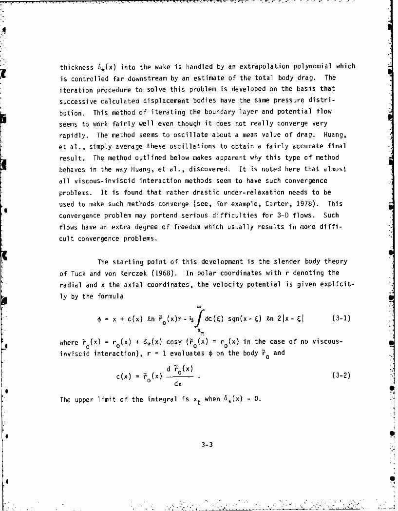
The starting point of this development is the slender body theory

of Tuck and von Kerczek (1968). In polar coordinates with r denoting the

radial and x the axial coordinates, the velocity potential is given explicit-

ly by the formula

= x + c(x) kn o(X)r- jdc( ) sgn(x- ) kn 21x- E (3-1)

X n

where ro(X) = r0 (X) + 6,(x) cosy (Fo(X) ro(X) in the case of no viscous-

inviscid interaction), r = 1 evaluates q on the body ro and

d i o(X)

c(x) X) d (3-2)0 dx

The upper limit of the integral is xt when 6,(x) =0.

3-3

|. °. \ •, . *

It should be noted that if the body has a blunt tail the potential

(3-3) is very singular there, and hence the boundary layer on such bodies

separates. This could prevent any viscous-inviscid interaction method from

converging because a separated flow is not a suitable first guess. This

can be overcome by artificially extending the body into the wake. This pro-

cedure can be carried out by the same method that is described below for

extending the displacement surface into the wake. Thus, a way to obtain a

suitable starting boundary layer needs no further discussion.

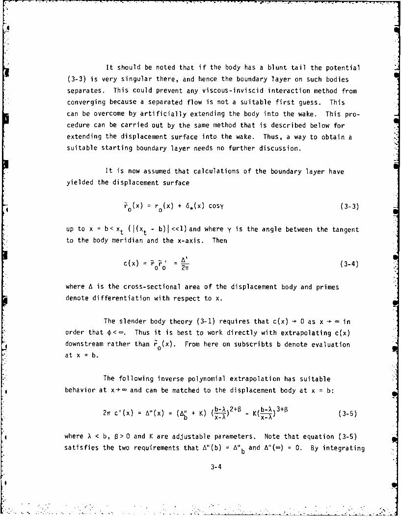
It is now assumed that calculations of the boundary layer have

yielded the displacement surface

0 (x) r0 (x) + 6,(x) cosy (3-3)

up to x = b< xt (I(xt - b)l<<1)and where y is the angle between the tangent

to the body meridian and the x-axis. Then

c(x) = ' -(3-4)0 o 2

where A is the cross-sectional area of the displacement body and primes

denote differentiation with respect to x.

The slender body theory (3-1) requires that c(x) - 0 as x in

order that *<. Thus it is best to work directly with extrapolating c(x)

downstream rather than ro(x). From here on subscribts b denote evaluation0

at x = b.

The following inverse polynomial extrapolation has suitable

behavior at x-- and can be matched to the displacement body at x = b:

b-X 2+B f- +27r c'(x) A"(x) : (Al + K) -, , - _x )'+ (3-5)

where X < b, >O and K are adjustable parameters. Note that equation (3-5)

satisfies the two requirements that A"(b) = Alb and A"(-) = 0. By integrating

3-4

4

equation (3-5) twice and matching to the displacement body at x b, the

wake displacement body i(x) is obtained. Thus,

2rrc(x) = A' (x) = (Ab+K)(b-X) b-X, 1++ K(b-,) b- 2+(3-~(1+S) x-AX (2+) x( -j- (3-6)

and(All+K) (b-X)2

A(x)= Ab + [(x-) 3 1(1+)(3-7)

K(b-X) 2 - +- 8)2+)[(b-x ') +(3 - 1]

where

K = - 2 (b-A) A + (1+3) AJ. (3-8)

The evaluation of equation (3-7) for x-- yields the relationship

between ACt and Ab, namely2 b-2 1(3(+3

A =Ab + *(b-X) A, + 1 (b- 2 Al (3-9)

This extrapolated wake is C2 continuous (i.e., A, A', A" are continuous) at

x = b. Thus, since the quantities Ab, A, and A" are computed by boundary

layer theory it is expected that wake (3-7) is an accurate approximation of

the wake in a significant neighborhood of the point x = b. If equation (3-7)

departs significantly from the asymptotic shape of the wake, the departure

should not have too much of an effect on the potential flow velocities up-

stream of and at the point b.

It is known (see Schlichting, 1979) that the far wake displacement

area A. is related to the drag coefficient CD of the body by the equation

A °CD' (3-10)

where Ao is the body reference area. Hence, equation (3-9) yields the rela-

tionship

3-5

8 4 2

Ao C D = 4Ab + (b-A) Ab + (1+g)(2+3) (b-A) A (3-11)

which will be the basis of the iteration procedure for calculating the vis-

cous-inviscid interaction.

However, before describing this iteration procedure in detail it

is best to carry equation (3-11) a little further. The axisymmetric momen-

tum integral boundary layer equations are the following:

dO + O(2+H) 1 dU r r (3-12a)T-s s 0 oX f

ds Q I dU_ (6cosy + r ) F(G) (3-12b)

where 0 is the momentum area, H = A,/O, A* is the displacement area (note

A* / A), Q = OG, G is Head's shape parameter, s is arclength along a body

meridian, cf is the skin friction coefficient, F is the entrainment rate and

U is the potential flow speed on the displacement body. See K for the

details of these boundary layer equations. The arclength s and the axial

coordinate x are related by

ds = 1 + r'(x)2 dx. (3-13)

In the vicinity of the tail of the body

r r0 0O

c 0f

ds dx (or Yb dx)

and

H constant = Hb.

3-6

du-~~~~ W7 -7 | Z

Thus, the momentum equation (3-12a) reduces there to the equation

A' + A(2+Hb) U'/U 0. (3-14)

By evaluating this equation at x = b, the following relationships are

obtained:

(2+Hb) UIA -A b (3-15a)b Ub

and

(2+H) 2

A" - [U Ub + (3+Hb) Ub JA . (3-15b)

b

Hence, equation (3-11) can be rewritten as

2 (2+Hb

A0 CD = 4 Ab 1 (b-X) -+UHUb

(b-A)2 (2+Hb) ( 3+Hb) U 2 U' Ub]}-+ b (3-16)(I+ ) (2+0) U2

Equation (3-16) clearly brings out the direct and seemingly sensitive

dependence of CD on Ub" U and Ub In fact, it seems likely that a good

choice of X is such that (b-A) = , say, and that probably B = 0(1). Then

the third term in equation (3-16) is probably negligible. It is then fairly

easy to see that viscous-inviscid iteration schemes will oscillate at each

iteration. Equation (3-16) is approximately the same as

(2+Hb):

Ao CD :4 Ab(l- (Hb) (3-17)0Db' Ub

and under the same assumptions, equation (3-11) is approximated by

8

A° CD 4 Ab + A . (3-18)

3-7

. ::", -" "-.'-" . '- . -"-'- -" - :- . .' . - -.-. .. .- - . - . .• - --. :I.

Assume that n is the iteration number. If at iteration n the

value of A' > 0, then it will produce a new velocity U' n+l> 0. Then if this

new velocity distribution for which Ub n+>0 is used to recalculate the

boundary layer, producing A~n+i, then by equations (3-17) and (3-18) (and

also simple physical reasoning) it is evident that A <n+ 0. Thus, it is

apparent that viscous-inviscid iteration will always lead to oscillatory

convergence (or divergence).

It is now worthwhile to state the iteration algorithm for viscous-

inviscid interaction calculations.

Step 0: Wr(X) = {r ° (x) XnX-<Xt}0 x >x t

t

If body is very blunt at the tail, possibly causing boundary layer

separation, add an artificial tail to the body using wake formulas

(3-5) - (3-7) with b = xt - 6, E>0, rob = o(xt - ) and c =

c'(xt - c) and replacing io(X) = 0 with W(x) = this artificial

tail for x>x t -

Calculate potential flowon this body (either exact or by slender

body theory or a combination of these).

Step 1: Calculate boundary layer on body r (X) to x = b to get A(x) and! A 0 0

Ab, Ab' Ab"

Step 2: Construct wake function using A Ab , A" and calculate CD fromAbb b0

formula (3-11). Is CD = CD from previsou iteration? (if on first

step go to 3) Yes; go to step 4. No; go to step 3.

Step 3: Calculate U by slender body theory potential (3-1) using A(x) on

body/wake from steps 1 - 2. Go to step 1.

Step 4: Calculate CD by stress integration. If CD is same as wake CD

problem is finished. If not, adjust X(or 0) so that the two values

of CD are equal and restart at step 2.

3-8

-"4 ' -. .- 3- .i " ' -. . - - . ."- - .;. . ' . . . - -.-. '.-. ' . , ..-.- 'i . - -- ; - .

3.3 Three-Dimensional Viscous-Inviscid Interactions

The beauty of the theory outlined in the previous subsection is

that it can be applied with only minor modifications to a ship hull. The

starting point of this development is the representation of a ship hull by

conformal mapping functions (von Kerczek and Tuck, 1969) and the general

ship slender body theory (Tuck and von Kerczek, 1968).

The ship hull is given by r=1 in the equation

r o(x,O,r) = xi + y(x,O,r)j + z(x,O,r)k. (3-19)

4 In equation (3-19)

N (3-2n)y + iz an(X) (3-20)

nwhere n=i

= re i0

and an(x) are interpolation functions along the axis of the ship.

The slender body velocity potential *(x,r,e) is obtained directly

in terms of the coefficient functions an(X) by the following formulas:

(Tuck and von Kerczek, 1968)

x+ C(x) kn a(x)c - N-c= 2n

r CO (3-21)

12 d c0 (E) sgn(x-&) £n2Ix-&j

where the coefficients cn(x), n = 0, ... , N are obtained from the formulas

c (Yn + Y ) e (3-22a)

N-nYn= 1 (3-2ax) a+n (X) (3-22b)

k=1

3-9

"1

i .

- - I *

for n 0en I forn>0 (3-22c)

and an (x) E 0 for n<1 and n>N.

The potential (3-22) splits into two important and distinct parts.

The first three terms of equation (3-22) are local. They only depend on

the particular point on the hull at which the velocity is evaluated. It is

only this local group of terms that contains the entire non-axisymmetry of

the hull shape. The integral in equation (3-22) is the only term that con-

veys the global aspects of the hull to each point on the ship. This term

is exactly the same as in the axisymmetric case. The function cC(x) is the

x-derivative of the cross-section area divided by 27r. Thus, the effects of

the wake are felt on the hull only by its section area distribution, notits cross-section shape. This feature of slender body theory is the crucial

element that makes the axisymmetric interaction theory easily extendable to

three dimensions.

After the boundary layer is calculated, a displacement thickness

distribution 6,(x,O) is obtained. Since this displacement thickness is

supposed to represent a distance normal to the hull, the equivalent distance

normal to the cross section out to the effective displacement surface is

given by 6,c(x,O) where

Sc(X,O) = 6,(x,O)(n • ), (3-23)

where n is the unit normal vector to the hull and n is the unit normalC

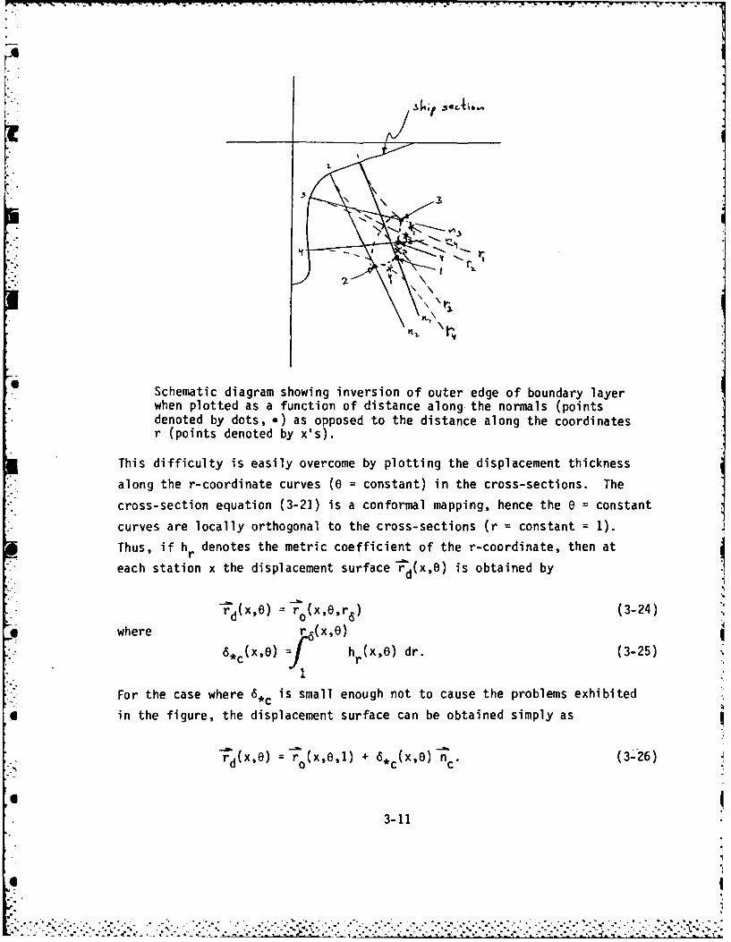
vector to the cross-section. Furthermore, near the stern the value of 6, c

may be so large that if this distance is plotted normal to the cross-section,

the neighboring displacement distances would cross, as sketched in the figure S

below.

3-10

. ....4

33

3

6Schematic diagram showing inversion of outer edge of boundary layerwhen plotted as a function of distance along the normals (pointsdenoted by dots, e) as opposed to the distance along the coordinatesr (points denoted by x's).

This difficulty is easily overcome by plotting the displacement thickness

along the r-coordinate curves (0 = constant) in the cross-sections. The

cross-section equation (3-21) is a conformal mapping, hence the 0 = constant

curves are locally orthogonal to the cross-sections (r = constant = 1).

Thus, if hr denotes the metric coefficient of the r-coordinate, then at

each station x the displacement surface rd(x,O) is obtained by

'_(xe -=i(x,', r6) (3-24)

where r6 (x,e)

6*c(X'O) =f hr(xE) dr. (3-25)

For the case where 6*c is small enough not to cause the problems exhibited

in the figure, the displacement surface can be obtained simply as

d(Xre) r 0 + (x,e) n . (3-26)

3-11

- m- -v .---- .

Once the surface (x,O) for x[a,b] has been constructed, then the

cross-sections of this surface are mapped onto the unit circle (using the

von Kerczek-Tuck, 1969, algorithm) and a new set of 4apping coefficients

a (x) is obtained. From these coefficients the new set of coefficients

Cn (x) are computed by formulas (3-22).

Now the section area derivative c (x) must be extrapolated to

infinity to complete the data for the potential (3-21). Again formulas

(3-5) - (3-11) are used for the wake. The same algorithm that was used for

the axisymmetric wake can now be used. Of course, the fully 3-D boundary

layer calculation method of K (or any other 3-D boundary layer method) must

be used to obtain the new effective displacement thickness 6,(x,e).

The beauty of this method is that the actual cross-section shape

of the wake need not be known as long as the potential flow velcoity on

the wake displacement surface does not have to be computed. This is pre-

cisely what is achieved by extrapolating the wake cross-section area.

Slender body theory makes this possible. It should be emphasized that this

theory does not assume that the wake is axisymmetric. Use of slender body

theory for the potential flow simply obviates the necessity to know the

cross-section shape of the wake. This method for doing three-dimensional

viscous-inviscid interaction seems extremely promising. Implementation of

the method to bring it to fruition is planned.

3-12

.. . . . . . . , . . C. . . . . . . . . .. . . . . . .

4.0 COMPUTATIONAL IMPROVEMENTS TO THE BASIC MOMENTUM INTEGRAL METHOD

It was found, in the course of several applications of the method

K, that the integration of the boundary layer equations broke down prematurely

near the stern. This breakdown was traced to -wo causes. The first cause

was an inadequate handling of the equations on the symmetry plane. The

second cause was the requirement in the original program that the boundary

layer equations be integrated with an axial step size conforming to the

potential flow panels. The remedies to these difficiencies which required

considerable effort are described below.

The original computer program of K (see von Kerczek, 1983) imple-

mented the symmetry plane conditions by appropriate parity of the finite

difference formulas on these planes (the load waterline and keel). It was

found that this kind of implementation of symmetry plane conditions allows

the boundary layer solution off the symmetry plane to affect the sym-

metry plane solution. But boundary layer theory indicates that the flow

along a symmetry plane is completely independent of the flow elsewhere on

the body (unless viscous-inviscid interactions are present). Hence, the

symmetry plane boundary layer equations must be solved independently of the

rest of the boundary layer and the results must be used as lateral boundary

conditions to the full three-dimensional equations. This method of handling

the symmetry planes has now been implemented in the method of K and results

in improved predictions of the boundary layer.

fl. The original computer program for the method of K used axial step

sizes fixed to the potential flow panels. The potential flow panels cannot

be made small enough at a ship stern to accommodate the requirements of the

* boundary layer equations unless an enormously expensive potential flow cal-

culation can be tolerated. This problem was alleviated by writing a pre-

processor that interpolates the potential flow data onto an arbitrary grid.

This decouples the numerical algorithm for solving the boundary layer equa-

* tions from the potential flow panels. The boundary layer equations in K can4

V 4-1

now be integrated on very fine step sizes near the stern of a ship. This

greatly improves the performance of the code of K. For example, the bound-

ary layer can now be computed to within 2% of ships' length to the stern of

the semi-elliptic hull of Huang, et al. (1976). Comparison of such calcu-

lations with the experimental data of Huang, et al. is not shown here

because the experiments had insufficient detail to allow the discernment of

an appropriate set of initial conditions to start the calculations. The

calculations that were made used rough guesses for initial conditions, and

thus the results, though qualitatively correct, are not comparable to the

experimental data.

It is planned that the SSPA model boundary layer (see K) will be

recalculated and compared to experiment with the improved code described

above.

4-2

"i . . .. -, ,' .'. -... .. .:. . .. . .. . . . . . . . ,-. . . . . . . .-- .- ,*.-, -.* . .- . .- - -, ..-.. ..- ., ,

APPENDIX: UNSUCCESSFUL METHOD FOR CALCULATING VISCOUS-INVISCID

INTERACTING AT A STERN

A brief outline is given here describing an unsuccessful idea for

calculating the stern flow of ships. This outline is given mainly to illus-

trate the difficulties that are inherent in trying to join computationally

the boundary layer and near wake calculations. The difficulties lie mainly

in trying to match up two geometrically dissimilar regions. It was shown

in Section 3 that a viscous-inviscid interaction scheme will be very sensi-

tive to the potential flow velocity and its first two derivatives. This

forebodes difficulties for any method that attempts to actually match up

surfaces in three dimensions.

The idea in the first attempt to do viscous-inviscid interactions

was to model the displacement effects by a distribution of extra sources on

the body and its extension in the wake. This attempt was carried out on the

Groves, etal. (1982) semi-elliptic body.

The body was truncated at a station xt - c, O<Pe<< 1, and an ellip-

tic cross-section tail cone was attached there. This tail cone extended a

distance downstream determined at x xt - E by the slopes of the waterline

and keel of the actual body.

The first iteration calculated the full three-dimensional bare

body boundary layer up to station xt - c. At station xt - e onwards the

wake was computed on the waterlineand keel of the extended tail cone.

The centerline pressure distribution behind the body without the tail cone

was used for the wake calculation. The tail cone only serves the purpose

of providing a continuation of the coordinate system off the end of the body.

This boundary layer and wake calculation then provides the displace-

ment surface 6,(x,O) (using the coordinates of section 3.2 say). Extra

A-i

S*!

• .', ; . .. • . . . " ," . .*_ - . , . . . *k_. - L i.m . i W ~

sources, :a-U (A-i)

where s is the arclength along the streamlines, were then distributed onI

the body and its extension. The increment to the original exact bare body

potential flow was then computed by slender body theory. Using this new

potential flow, the boundary layer and wake were recalculated.j

The method failed because of extremely erratic behavior of the

potential flow and the extra source strengths a in the neighborhood of thetail of the body. Examination of the details of this method did not leadIto optimism towards a continuation of this technique, so it was abandoned.

The lesson learned here is that it is very tricky to actually con-

tinue a three-dimensional body, even a displacement body, into the wake.The reason is that the potential flow is so sensitive to inflection points(i.e., in naval architectural terms, the fairness of the body) that it is

too difficult to extend surfaces in three dimensions. The slender body

method outlined in section 3.2 only requires that a curve be continued

downstream, namely the section area curve. This is the same as what is

required in the axisymmetric case, and this has been shown to work by

Huang, et al. (1976).

A- 2

R D. .66 T

REFERENCES

*Betterman, 0. (1966) "Contribution a l'Etude de la Connection ForcesTurbulente le long Plaques Rugueuses," Int. J. Heat & Mass Transfer,Vol. 9, pp. 153-164.

Carter, J.E. (1978) "A New Boundary Layer Interaction Technique forSeparated Flows," NASA-TM-78690.

Christoph, G.H., and R.H. Pletcher (1983) "Prediction of Rough-Wall SkinFriction and Heat Transfer," AIAA Journal, Vol. 21, No. 4, pp. 509-515.

Dirling, R.B., Jr. (1973) "A Method for Computing Roughwall Heat TransferRates on Re-entry Nosetips," AIAA Paper No. 73-763, presented at theAIAA 8th Thermophysics Conference, Palm Springs, CA, 16-18 Jul 1973.

Finson, M.L. (1982) "A Model for Rough Wall Turbulent Heating and SkinFriction," AIAA Paper No. 82-0199, presented at AIAA 20th AerospaceSciences Meeting, Orlando, FL, 11-14 Jan 1982.

Finson, M.L., and A.S. Clarke (1980) "The Effect of Surface RoughnessCharacter on Turbulent Re-entry Heating," AIAA Paper No. 80-1459.

Granville, P.S. (1974) "A Modified Froude Method for Determining FullScale Resistance of Surface Ships from Towed Models," J. Ship Res.,Vol. 18, No. 4.

Groves, N.C., G.S. Belt and T.T. Huang (1982) "Stern Boundary Layer Flowon a Three-Dimensional Body of 3:1 Elliptic Cross Section," Report#DTNSRDC-82/022.

Healzer, J.M., R.J. Moffat and W.M. Kays (1974) "The Turbulent BoundaryLayer on a Porous Rough Plate: Experimental Heat Transfer withUniform Blowing," AIAA Paper No. 74-680 and ASME Paper No. 74-HT-14,presented at the AIAA/ASME 1974 Thermophysics and Heat Transfer Con-ference, Boston, MA, 15-17 Jul 1974.

Hogan, T.F. (1983) "A Calculation of the Parabolized Navier-StokesEquations for Turbulent Axisymmetric Flows Using Streamline Coor-dinates and the k-c Turbulence Model," DTNSRDC Report #83/070.

Huang, T.T., et al. (1976) "Propeller/Stern/Boundary-Layer Interactionon Axisymmetric Bodies: Theory and Experiment," DTNSRDC Report

#76/0113.

R-1

.S

-

Larsson, L. (ed.) (1981) "SSPA-ITTC Workshop on Ship Boundary Layers 1980,"SSPA, Goteborg, Report No. 90.

Lin, T.C., and R.J. Bywater (1982) "Turbulence Models for High-speed,Rough-wall Boundary Layers," AIAA Journal, Vol. 20, No. 3, pp. 325-333.

Patel, V.C. (1983) "Some Aspects of Thick Three-Dimensional BoundaryLayers," Proc. 14th Symp. Naval Hydrodynamics, National Academy Press,Washington, D.C.

Schlichting, H. (1937) "Experimental Investigation of the Problem of

Surface Roughness," NACA TM823.

Schlichting, H. (1969) Boundar _Layer Theory, McGraw-Hill, New York.

Simpson, R.L. (1973) "A Generalized Correlation of Roughness DensityEffects on t~e Turbulent Boundary Layer," AIAA Journal, Vol. 11,No. 2, pp. 224-244.

Stern, F., and C. von Kerczek (1983) "Calculation of Appendage Drag andPropeller Inflow for Destroyer Hull Forms," NAVSEA Tech. Note 051-55W-TNO002.

Tuck, E.O., and C. von Kerczek (1968) "Streamlines and Pressure Distribu-tion on Arbitrary Ship Hulls at Zero Froude Number," J. Ship Res.,Vol. 12, No. 3.

von Kerczek, C.H. (1982) "A New Generalized Cross-Flow Momentum IntegralMethod for Three-Dimensional Ship Boundary Layers," SAI Report #463-82-085-LJ.

von Kerczek, C.H. (1983) "A User's Manual for the Ship Boundary LayerProgram GHRBLD," Supplement to SAI Report #463-82-085-LJ for Contract#N00014-81-C-0234.

von Kerczek, C., and T. Langan (1979) "An Integral Prediction Method forThree-Dimensional Turbulent Boundary Layers on Ships," DTNSRDC Report#79/006.

von Kerczek, C., C. Scragg and F. Stern (1983) "A Comparative Study ofthe Resistance of Two Destroyer Hull Forms," NAVSEA Technical Note#051-55W-TNOOO1.

von Kerczek, C., and E.O. Tuck (1969) "The Representation of Ship Hullsby Conformal Mapping Functions," J. Ship Res., Vol. 13, No. 4.

R-2

- .

FILMED

4-85

DTICI7 e