FUNDAMENTAL STUDY OF HEAT PIPE DESIGN FOR HIGH HEAT FLUX SOURCE

Ryoji Oinuma, Frederick R. Best Department of Nuclear Engineering, Texas A&M University

ABSTRACT

As the demand for high performance small electronic devices has increased, heat

removal from these devices for space use is approaching critical limits. A loop heat

pipe(LHP) with coherent micron-porous evaporative wick is suggested to enhance the

heat removal performance for the limited mass of space thermal management system.

The advantage of LHPs to have accurate micron-order diameter pores which will give

large evaporative areas compared with conventional heat pipes per unit mass. Also this

design make it easy to model the pressure drop and evaporation rate in the wick

compared with the evaluation of the heat pipe performance with a stochastic wick. This

gives confidence in operating limit calculation as well as the potential for the ultra high

capillary pressure without corresponding pressure penalty such as entrainment of the

liquid due to the fast vapor flow. The fabrication of this type heat pipe could be

achieved by utilizing lithographic fabrication technology for silicon etching. The

purpose of this paper is to show the potential of a heat pipe with a coherent

micron-porous evaporative wic k from the view point of the capillary limitation, the

boiling limitation, etc. The heat pipe performance is predicted with evaporation models

and the geometric design of heat pipe is optimized to achieve the maximum heat

removal performance per unit mass.

INTRODUCTION

In recent years, the high thermal performance requirements for integrated circuits in

computers, telecommunications, networking, and power -semiconductor markets are

making high heat flux( 2/100 cmW> ) and improved thermal management critical needs.

Heat pipes are promising devices to remove thermal energy and keep the integrated

circuits at the proper working temperature. The advantage of the heat pipe is in using

phase change phenomena to remove thermal energy since the heat transfer coefficient of

the phase change is normally 10-1000 times larger than typical heat transfer methods

such as heat conduction, forced vapor or liquid convection. Even though a heat pipe has

a big potential to remove the thermal energy from a high heat flux source, the heat

removal performance of heat pipes cannot be predicted well since a first principles of

evaporation has not been established.

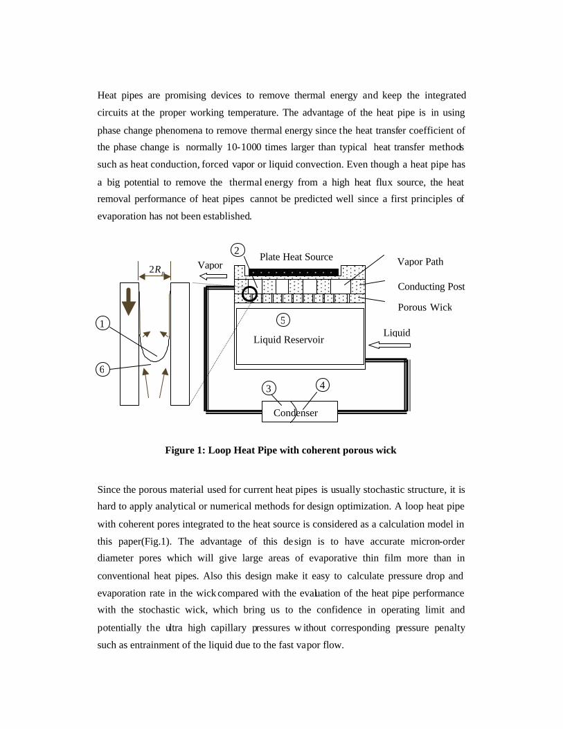
Figure 1: Loop Heat Pipe with coherent porous wick

Since the porous material used for current heat pipes is usually stochastic structure, it is

hard to apply analytical or numerical methods for design optimization. A loop heat pipe

with coherent pores integrated to the heat source is considered as a calculation model in

this paper(Fig.1). The advantage of this design is to have accurate micron-order

diameter pores which will give large areas of evaporative thin film more than in

conventional heat pipes. Also this design make it easy to calculate pressure drop and

evaporation rate in the wick compared with the evaluation of the heat pipe performance

with the stochastic wick, which bring us to the confidence in operating limit and

potentially the ultra high capillary pressures w ithout corresponding pressure penalty

such as entrainment of the liquid due to the fast vapor flow.

Liquid Reservoir

Porous Wick

Vapor

Liquid

Condenser

Conducting Post

Vapor Path Plate Heat Source

1

2

3 4

pR2

5

6

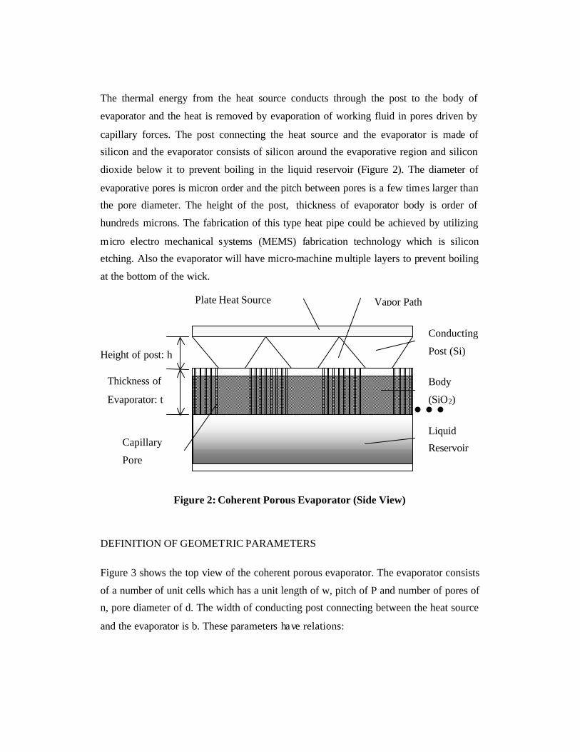
The thermal energy from the heat source conducts through the post to the body of

evaporator and the heat is removed by evaporation of working fluid in pores driven by

capillary forces. The post connecting the heat source and the evaporator is made of

silicon and the evaporator consists of silicon around the evaporative region and silicon

dioxide below it to prevent boiling in the liquid reservoir (Figure 2). The diameter of

evaporative pores is micron order and the pitch between pores is a few times larger than

the pore diameter. The height of the post, thickness of evaporator body is order of

hundreds microns. The fabrication of this type heat pipe could be achieved by utilizing

micro electro mechanical systems (MEMS) fabrication technology which is silicon

etching. Also the evaporator will have micro-machine multiple layers to prevent boiling

at the bottom of the wick.

Figure 2: Coherent Porous Evaporator (Side View)

DEFINITION OF GEOMETRIC PARAMETERS

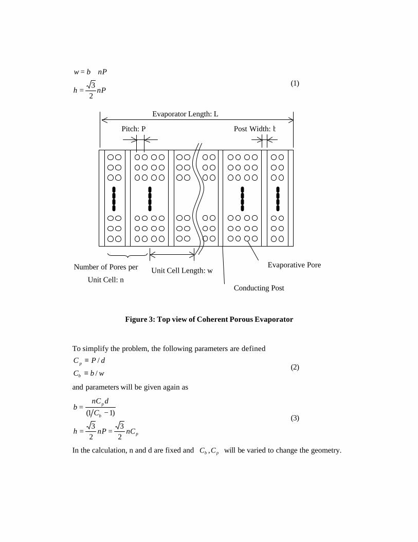
Figure 3 shows the top view of the coherent porous evaporator. The evaporator consists

of a number of unit cells which has a unit length of w, pitch of P and number of pores of

n, pore diameter of d. The width of conducting post connecting between the heat source

and the evaporator is b. These parameters have relations:

Conducting

Post (Si)

Capillary

Pore

Liquid

Reservoir

Body

(SiO2)

Vapor Path Plate Heat Source

Thickness of

Evaporator: t

Height of post: h

nPh

nPbw

23

=

+= (1)

Figure 3: Top view of Coherent Porous Evaporator

To simplify the problem, the following parameters are defined

wbC

dPC

b

p

/

/

≡

≡ (2)

and parameters will be given again as

p

b

p

nCnPh

C

dnCb

23

23

)11(

==

−=

(3)

In the calculation, n and d are fixed and pb CC , will be varied to change the geometry.

Conducting Post

Evaporative Pore

Pitch: P Post Width: b

Evaporator Length: L

Number of Pores per

Unit Cell: n Unit Cell Length: w

METHOD

OVERVIEW OF CALCULATION

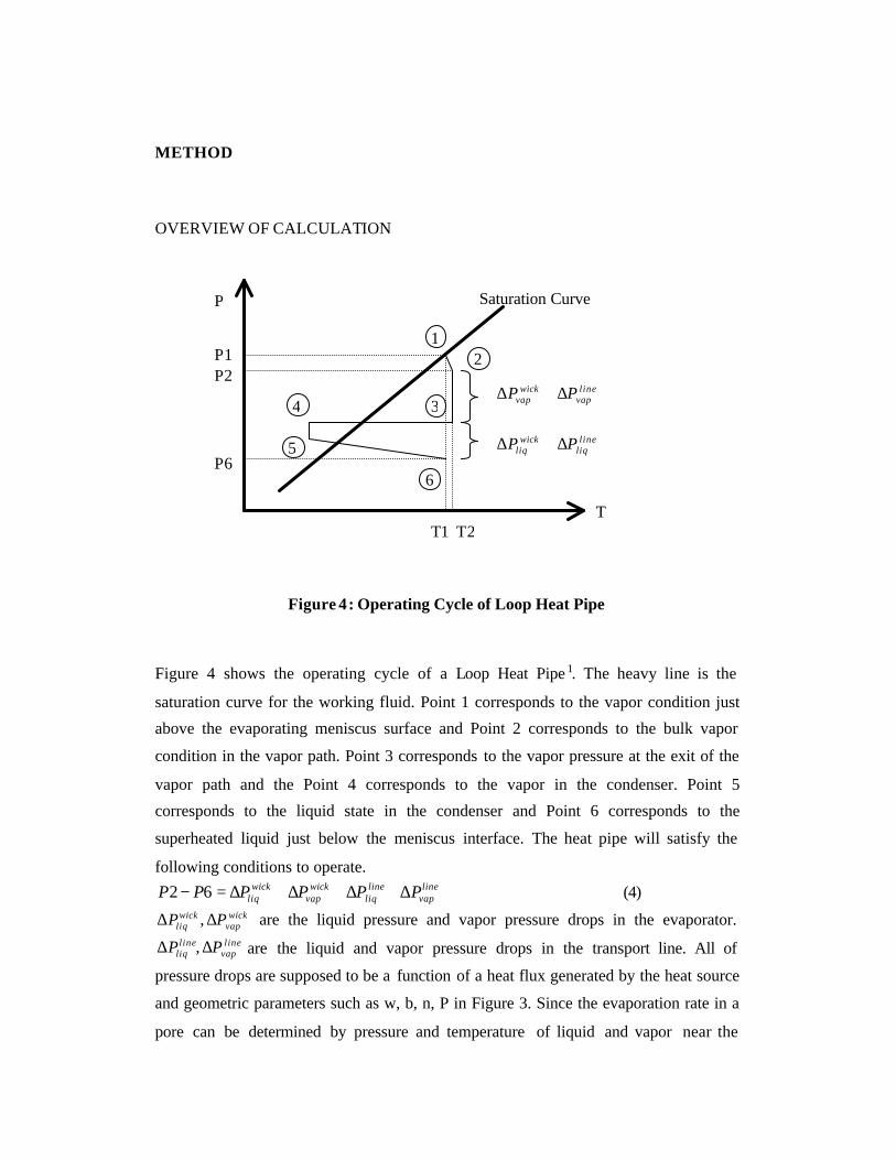
Figure 4: Operating Cycle of Loop Heat Pipe

Figure 4 shows the operating cycle of a Loop Heat Pipe 1. The heavy line is the

saturation curve for the working fluid. Point 1 corresponds to the vapor condition just

above the evaporating meniscus surface and Point 2 corresponds to the bulk vapor

condition in the vapor path. Point 3 corresponds to the vapor pressure at the exit of the

vapor path and the Point 4 corresponds to the vapor in the condenser. Point 5

corresponds to the liquid state in the condenser and Point 6 corresponds to the

superheated liquid just below the meniscus interface. The heat pipe will satisfy the

following conditions to operate. line

vapline

liqwick

vapwick

liq PPPPPP ∆+∆+∆+∆=− 62 (4) wick

vapwick

liq PP ∆∆ , are the liquid pressure and vapor pressure drops in the evaporator. line

vapline

liq PP ∆∆ , are the liquid and vapor pressure drops in the transport line. All of

pressure drops are supposed to be a function of a heat flux generated by the heat source

and geometric parameters such as w, b, n, P in Figure 3. Since the evaporation rate in a

pore can be determined by pressure and temperature of liquid and vapor near the

linevap

wickvap PP ∆+∆

T

P

lineliq

wickliq PP ∆+∆

21

34

5

6

Saturation Curve

P1 P2

P6

T1 T2

interface, the evaporation rate in a pore is a function of these values. If we define the

effective evaporation rate per unit pore area, evapq ′′ , we will have a relation of

)(),,,()6,6,2,2( dAPnbwNTPTPqAq poreevapsourcesource ′′=′′ . (5)

sourceq ′′ is heat flux generated by the heat source. sourceA and poreA are the area of the

heat source and a pore. N is the total number of pore in an evaporator and will be given

as

nwPLN

2

= (6)

Since the area of a pore is a function of the diameter of pore and the number of the pore

is a function of geometry parameter of evaporator (Figure 3), N varies due to the

geometry of the evaporator. It will be assumed that the temperature increase(T2-T1) of

the steam in the vapor path due to the heat transfer from the conducting wall or the heat

source is small so that 261 TTT ≈= . We set T2=T6=constant. P6 is assumed to be

equal to the saturation pressure at the temperature of condenser(T5). This is ba sed on

the fact that Point 5 could not be far from the saturation curve and the pressure drop

from Point 5 to 6 is not large compared with the saturation pressure at T5. P2 will be

obtained for a provided geometry to satisfy equations (4) and (5). This chapter shows

the way to calculate the effective evaporation rate per unit pore area( evapq ′′ ) and the

pressure drops(P2-P6) to solve equations (4) and (5).

PHENOMENA IN A PORE

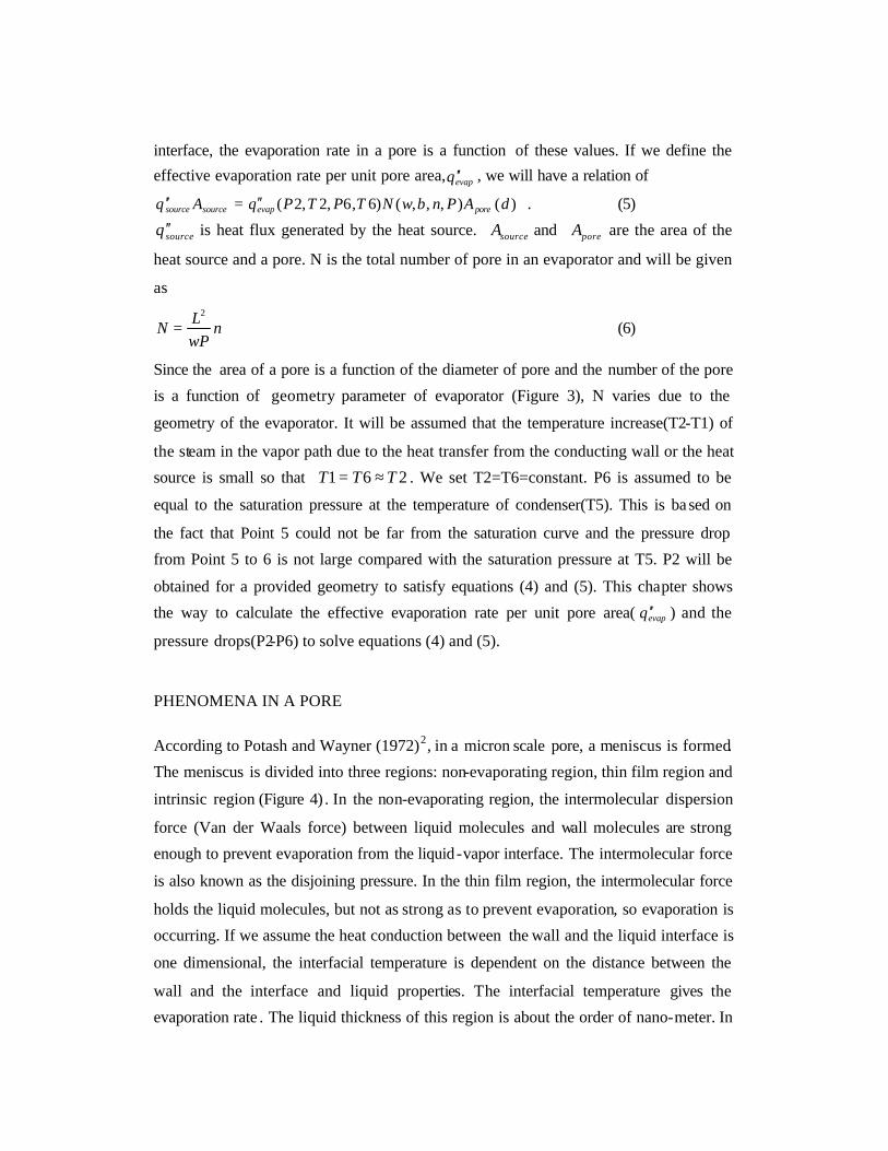
According to Potash and Wayner (1972)2, in a micron scale pore, a meniscus is formed.

The meniscus is divided into three regions: non-evaporating region, thin film region and

intrinsic region (Figure 4) . In the non-evaporating region, the intermolecular dispersion

force (Van der Waals force) between liquid molecules and wall molecules are strong

enough to prevent evaporation from the liquid -vapor interface. The intermolecular force

is also known as the disjoining pressure. In the thin film region, the intermolecular force

holds the liquid molecules, but not as strong as to prevent evaporation, so evaporation is

occurring. If we assume the heat conduction between the wall and the liquid interface is

one dimensional, the interfacial temperature is dependent on the distance between the

wall and the interface and liquid properties. The interfacial temperature gives the

evaporation rate . The liquid thickness of this region is about the order of nano-meter. In

the intrinsic meniscus region, the surface tension is dominant and the meniscus is

formed. The evaporation rate per unit area is relatively smaller than in the thin film

region.

Figure 4: Classification of Evaporating Region

GOVERNING EQUATION

The meniscus profile and the evaporation rate along the meniscus interface can be

calculated by solving Navier-Stokes equation (DasGupta, 1993) 3. The momentum

equation in Cartesian coordinate in the transition region is given by lubrication theory as

zP

yu l

∂∂

=∂∂

2

2

µ (7)

The boundary conditions are 0)( =poreRu at the wall and 0=∂∂ yu at the interface.

Integrating the momentum equation from )(xRy pore δ−= to poreRy = yields

{ }))(2())((221

)( 2 zRRyzRyzp

yu poreporeporel δδ

µ+−−+−+

∂∂

= . (8)

The mass flow rate at z=z will be

∫=

−==Γ

Rporey

zRporeydyyu

)()(

δρ . (9)

I : Non-Evaporating Region

II : Transient Region

III : Meniscus Region

pR2Thermal Energy

Evaporation

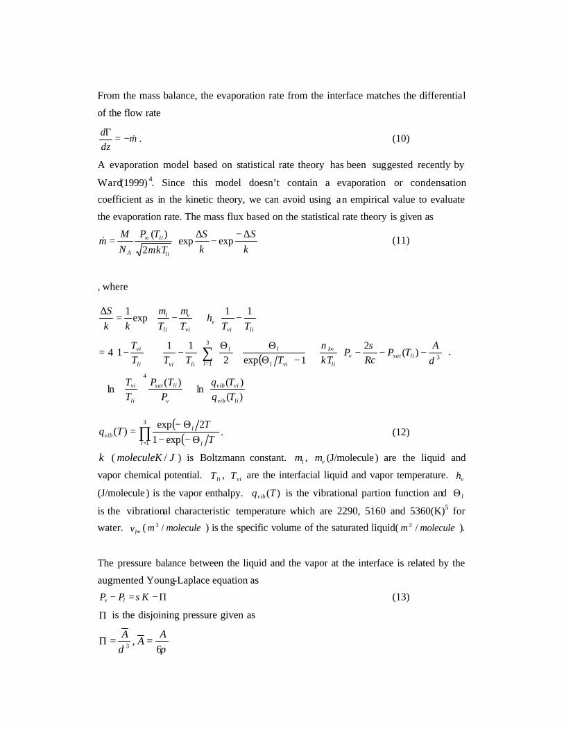
From the mass balance, the evaporation rate from the interface matches the differential

of the flow rate

mdzd &−=Γ . (10)

A evaporation model based on statistical rate theory has been suggested recently by

Ward(1999) 4. Since this model doesn’t contain a evaporation or condensation

coefficient as in the kinetic theory, we can avoid using an empirical value to evaluate

the evaporation rate. The mass flux based on the statistical rate theory is given as

∆−

−∆

= ∞

kS

kS

mkT

TPNM

mli

li

A

expexp2

)(& (11)

, where

( )

+

+

−−−+

−Θ

Θ+

Θ

−+

−=

−+

−=

∆

∑=

∞

)()(

ln)(

ln

)(2

1exp211

14

11exp

1

4

3

13

livib

vivib

v

lisat

li

vi

llisatv

li

l

vil

ll

livili

vi

liviv

vi

v

li

l

TqTq

PTP

TT

ATP

RcP

kTTTTTT

TTh

TTkkS

δσν

µµ

.

( )( )∏

= Θ−−Θ−

=3

1 exp12exp

)(l l

lvib T

TTq . (12)

k ( JmoleculeK / ) is Boltzmann constant. lµ , vµ (J/molecule ) are the liquid and

vapor chemical potential. liT , viT are the interfacial liquid and vapor temperature. vh

(J/molecule ) is the vapor enthalpy. )(Tqvib is the vibrational partion function and lΘ

is the vibrational characteristic temperature which are 2290, 5160 and 5360(K)5 for

water. ∞lv ( moleculem /3 ) is the specific volume of the saturated liquid( moleculem /3 ).

The pressure balance between the liquid and the vapor at the interface is related by the

augmented Young-Laplace equation as

Π−=− KPP lv σ (13)

Π is the disjoining pressure given as

πδ 6 ,3

AA

A==Π

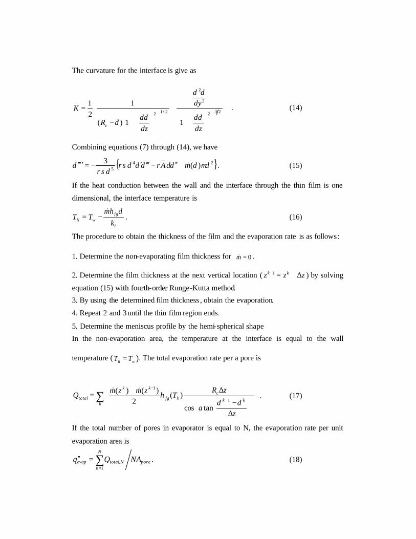
The curvature for the interface is give as

+

+

+−

= 232

2

2

2/12

11)(

121

dzd

dyd

dzd

R

K

c

δ

δ

δδ

. (14)

Combining equations (7) through (14), we have

{ }245 )(3 µδδδδρδδρσδ

ρσδδ mA &+′′−′′′′−=′′′′ . (15)

If the heat conduction between the wall and the interface through the thin film is one

dimensional, the interface temperature is

l

fgwli k

hmTT

δ&−= . (16)

The procedure to obtain the thickness of the film and the evaporation rate is as follows:

1. Determine the non-evaporating film thickness for 0=m& .

2. Determine the film thickness at the next vertical location ( zzz kk ∆+=+1 ) by solving

equation (15) with fourth-order Runge-Kutta method.

3. By using the determined film thickness , obtain the evaporation.

4. Repeat 2 and 3 until the thin film region ends.

5. Determine the meniscus profile by the hemi-spherical shape

In the non-evaporation area, the temperature at the interface is equal to the wall

temperature (wli TT = ). The total evaporation rate per a pore is

∑

∆

−

∆+=+

−

kkk

clifg

kk

total

za

zRThzmzmQ

δδ 1

1

tancos

)(2

)()( &&. (17)

If the total number of pores in evaporator is equal to N, the evaporation rate per unit

evaporation area is

pore

N

nNtotalevap NAQq ∑

=

=′′1

, . (18)

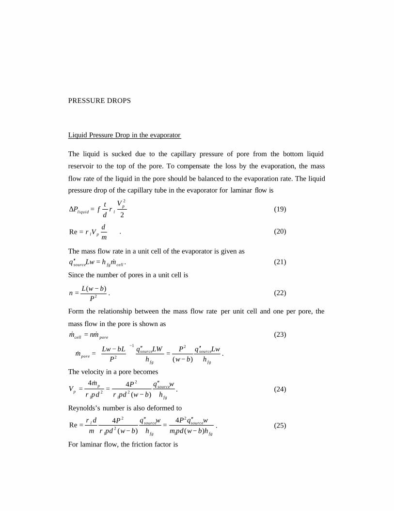
PRESSURE DROPS

Liquid Pressure Drop in the evaporator

The liquid is sucked due to the capillary pressure of pore from the bottom liquid

reservoir to the top of the pore. To compensate the loss by the evaporation, the mass

flow rate of the liquid in the pore should be balanced to the evaporation rate. The liquid

pressure drop of the capillary tube in the evaporator for laminar flow is

2

2p

lliquid

V

dt

fP ρ=∆ (19)

µρ

dV pl=Re . (20)

The mass flow rate in a unit cell of the evaporator is given as

cellfgsource mhLwq &=′′ . (21)

Since the number of pores in a unit cell is

2

)(P

bwLn

−= . (22)

Form the relationship between the mass flow rate per unit cell and one per pore, the

mass flow in the pore is shown as

porecell mnm && = (23)

fg

source

fg

sourcepore h

Lwqbw

Ph

LWqP

bLLwm

′′−

=′′

−=∴

−

)(

21

2& .

The velocity in a pore becomes

fg

source

ll

pp h

wqbwd

Pd

mV

′′

−==

)(442

2

2 πρπρ

&. (24)

Reynolds’s number is also deformed to

fgl

source

fg

source

l

l

hbwdwqP

hwq

bwdPd

)(4

)(4Re

2

2

2

−

′′=

′′

−=

πµπρµρ

. (25)

For laminar flow, the friction factor is

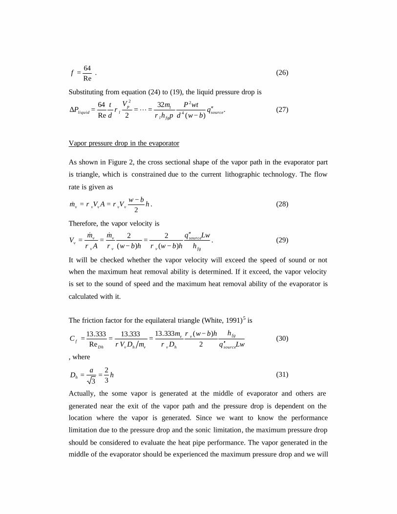
Re64=f . (26)

Substituting from equation (24) to (19), the liquid pressure drop is

sourcefgl

lplliquid q

bwdwtP

h

V

dt

P ′′−

===∆)(

322Re

644

22

πρµ

ρ L . (27)

Vapor pressure drop in the evaporator

As shown in Figure 2, the cross sectional shape of the vapor path in the evaporator part

is triangle, which is constrained due to the current lithographic technology. The flow

rate is given as

hbw

VAVm vvvvv 2−== ρρ& . (28)

Therefore, the vapor velocity is

fg

source

vv

v

v

vv h

Lwqhbwhbw

mA

mV

′′

−=

−==

)(2

)(2

ρρρ

&&. (29)

It will be checked whether the vapor velocity will exceed the speed of sound or not

when the maximum heat removal ability is determined. If it exceed, the vapor velocity

is set to the sound of speed and the maximum heat removal ability of the evaporator is

calculated with it.

The friction factor for the equilateral triangle (White, 1991)5 is

Lwq

hhbwDDV

Csource

fgv

hv

v

vhvDhf ′′

−===

2)(333.13333.13

Re333.13 ρ

ρµ

µρ (30)

, where

ha

Dh 32

3== (31)

Actually, the some vapor is generated at the middle of evaporator and others are

generated near the exit of the vapor path and the pressure drop is dependent on the

location where the vapor is generated. Since we want to know the performance

limitation due to the pressure drop and the sonic limitation, the maximum pressure drop

should be considered to evaluate the heat pipe performance. The vapor generated in the

middle of the evaporator should be experienced the maximum pressure drop and we will

calculate it. The path length for this vapor is 2L until the exit and the hydraulic

diameter for the equilateral triangle is given as 323 haDh ==

By using above equations, the vapor pressure drop is given as

v

hvV

sourcefgv

vvv

hfvapor

DV

qh

wLh

VDLCP

µρ

ρµ

ρ

=

′′===∆

Re

96.512

242

4

2

…. (31)

Vapor and Liquid Pressure Drop in Transport Line

The vapor and liquid pressure drop in the transport line are given as

sourcefgvv

vlinevap q

hDl

P ′′=∆πρ

µ4

32 , (32)

sourcefgllv

llineliq q

hDl

P ′′=∆πρ

µ4

32 . (33)

LIMITATION OF HEAT PIPE PERFORMANCE

There are some limits to control the heat transfer of heat pipes (Faghri 1995)1: Capillary

limitation, Sonic Limitation, Boiling Limitation, Viscous Limitation, Entrainment

Limitation. These give information of the heat transfer limit due to the parameters such

a pore diameter, a pitch between pores, number of pores between posts, thermophysical

properties of working fluid (Figure 3).

For instance, the total pressure drop in the system is supposed to be lower than the

capillary pressure to make the heat pipe work. The total pressure drop in the system is

given by the sum of the pressure drop of liquid in pore, vapor in the exiting path over

the evaporator, liquid and vapor transportation line to or from the condenser. line

vapline

liqwick

vapwick

liqcap PPPPP ∆+∆+∆+∆>∆ , (34)

If these pressure drops are expressed in geometric and thermophysical parameters of

working fluid stated above, the equation (34) is expressed as

1

44

2

44

2 323296.51)(

322−

+++

−<′′

fgll

l

fgvv

v

fgv

v

fgl

lsource hD

lhDl

hwL

hbwdhwtP

rq

πρµ

πρµ

ρµ

πρµσ ,

where bnPw += . (35)

lµ and vµ are the liquid and vapor viscosities, P is the pitch between pores, lρ

and vρ are the liquid and vapor densities, d is the diameter of pore, lD and vD

are the pipe diameter in the liquid and vapor transport lines, b and h are the width

and height of the conducting post, l is the length of transport line, L is the horizontal

length of evaporator, n is the number of pores between conducting posts. In the similar

way for other limitations, the heat transfer limit will be calculated with these

parameters.

TEMPERATURE DIFFERENCE BETWEEN HEAT SOUCE AND EVAPORATOR

Since the shape of vapor path is the right triangle, the height(h) can be determined if

other parameters such as P, n, d, b are known. Therefore, the shape of the conducting

post will be determined as well(Figure 2 and 3). The temperature difference between

heat source and evaporator is given as

++′′=∆

bhb

Lkh

bqTwall

sourcewall 3323

ln3

)3

2(5.0 . (36)

RESULT

GEOMETRY AND ASSUMPTIONS

We assume that we want to design the loop heat pipe which can remove the thermal

energy from a heat source which generates a uniform heat flux and has the size of 1cm

by 1cm, thus L=1cm. The evaporative pore diameter(d) is 10µm and the working fluid

is water. The number of pores per unit cell(n) is set to 10. The thickness of the

evaporator(t) is 200µm. Pitch between pores will be changed from dP 1.1= to

dP 6= and the width of conducting post(b) varies between wb 01.0= and

wb 09.0= . T2 is set to from 323.15 to 373.15K and P6 is assumed to be equal to the

saturation pressure at 300K( Pa4200≈ ). To simplify the problem, the temperature is

uniform for the horizontal direction, the thermal contact resistances at the connection

between the heat source and the conducting post or between the conducting post and the

evaporator are ignored. The heat loss from the heat source by the radiation and

convection is ignored also.

EVAPORATION AND MENISCUS PROFILE IN A PORE

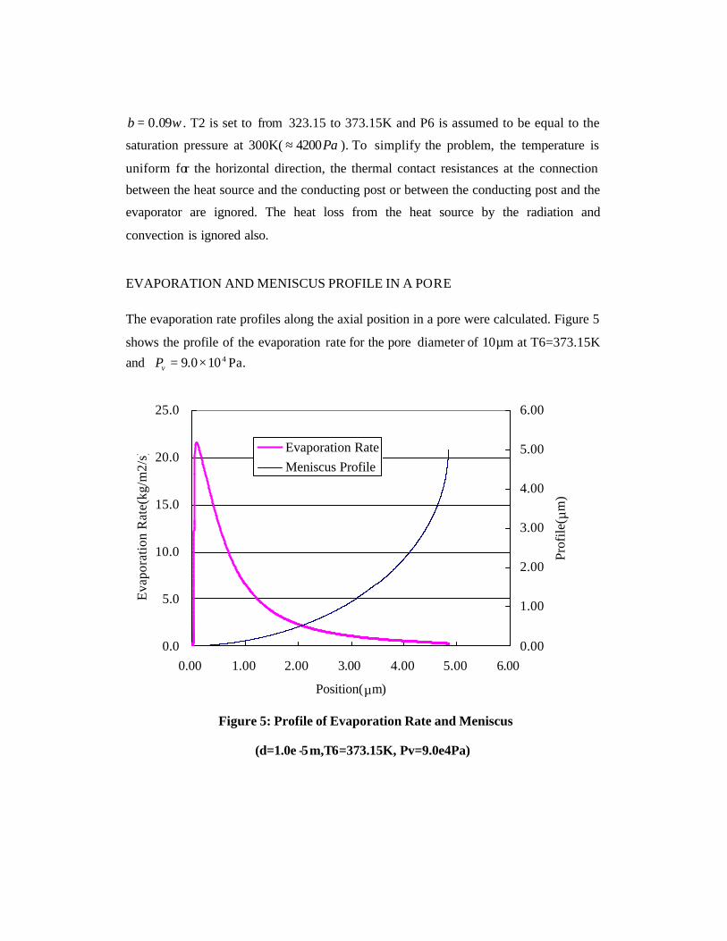
The evaporation rate profiles along the axial position in a pore were calculated. Figure 5

shows the profile of the evaporation rate for the pore diameter of 10µm at T6=373.15K

and 4100.9 ×=vP Pa.

0.0

5.0

10.0

15.0

20.0

25.0

0.00 1.00 2.00 3.00 4.00 5.00 6.00

Position(µm)

Eva

pora

tion

Rat

e(kg

/m2/

s)

0.00

1.00

2.00

3.00

4.00

5.00

6.00

Prof

ile( µ

m)

Evaporation RateMeniscus Profile

Figure 5: Profile of Evaporation Rate and Meniscus

(d=1.0e -5m,T6=373.15K, Pv=9.0e4Pa)

Vapor Pressure(Pa)

0.0 2.0e+4 4.0e+4 6.0e+4 8.0e+4 1.0e+5 1.2e+5Hea

t Rem

oval

Cap

abili

ty p

er u

nit p

ore

area

(W

/cm

2)

0

500

1000

1500

2000

2500

T6=373.15KT6=363.15KT6=353.15KT6=343.15KT6=333.15KT6=323.15K

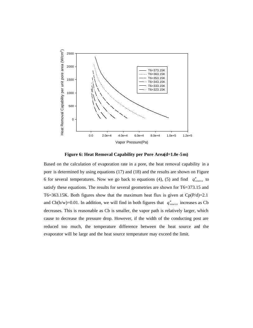
Figure 6: Heat Removal Capability per Pore Area(d=1.0e -5m)

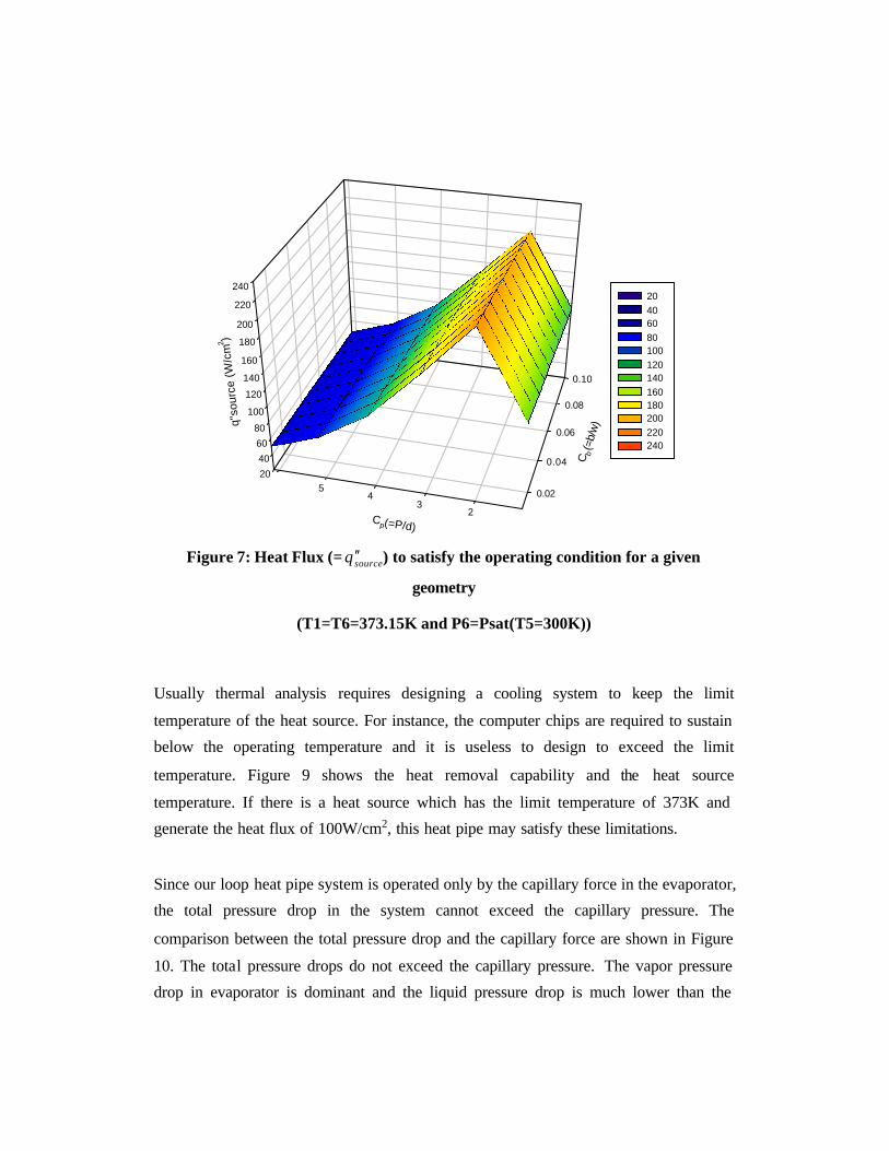
Based on the calculation of evaporation rate in a pore, the heat removal capability in a

pore is determined by using equations (17) and (18) and the results are shown on Figure

6 for several temperatures. Now we go back to equations (4), (5) and find sourceq ′′ to

satisfy these equations. The results for several geometries are shown for T6=373.15 and

T6=363.15K. Both figures show that the maximum heat flux is given at Cp(P/d)=2.1

and Cb(b/w)=0.01. In addition, we will find in both figures that sourceq ′′ increases as Cb

decreases. This is reasonable as Cb is smaller, the vapor path is relatively larger, which

cause to decrease the pressure drop. However, if the width of the conducting post are

reduced too much, the temperature difference between the heat source and the

evaporator will be large and the heat source temperature may exceed the limit.

20

40

60

80

100

120

140

160

180

200

220

240

0.02

0.04

0.06

0.08

0.10

23

45

q"so

urce

(W

/cm

2 )

C b(=

b/w

)

Cp(=P/d)

20 40 60 80 100 120 140 160 180 200 220 240

Figure 7: Heat Flux (= sourceq ′′ ) to satisfy the operating condition for a given

geometry

(T1=T6=373.15K and P6=Psat(T5=300K))

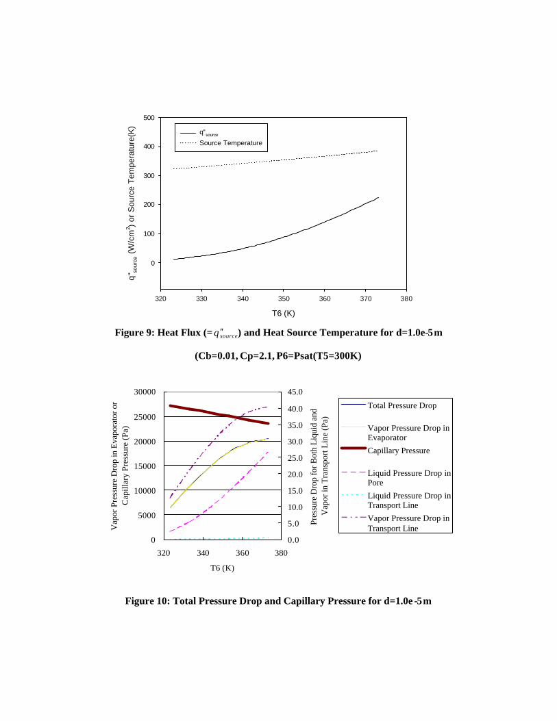
Usually thermal analysis requires designing a cooling system to keep the limit

temperature of the heat source. For instance, the computer chips are required to sustain

below the operating temperature and it is useless to design to exceed the limit

temperature. Figure 9 shows the heat removal capability and the heat source

temperature. If there is a heat source which has the limit temperature of 373K and

generate the heat flux of 100W/cm2, this heat pipe may satisfy these limitations.

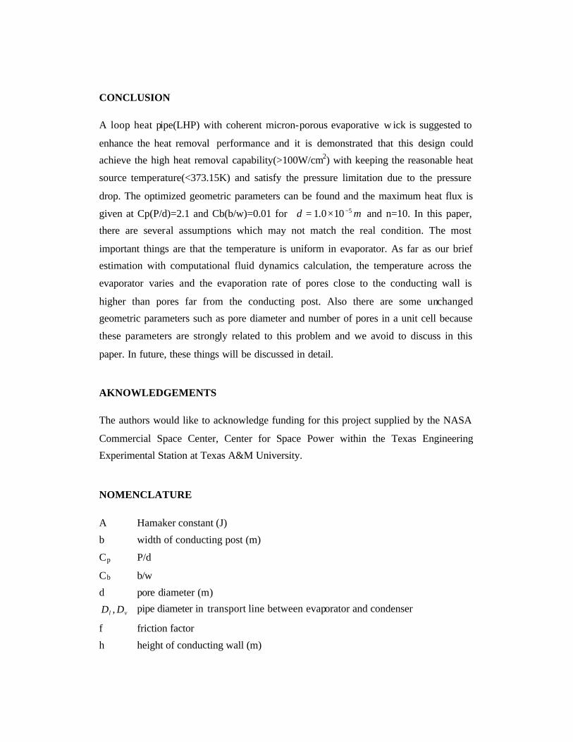
Since our loop heat pipe system is operated only by the capillary force in the evaporator,

the total pressure drop in the system cannot exceed the capillary pressure. The

comparison between the total pressure drop and the capillary force are shown in Figure

10. The total pressure drops do not exceed the capillary pressure. The vapor pressure

drop in evaporator is dominant and the liquid pressure drop is much lower than the

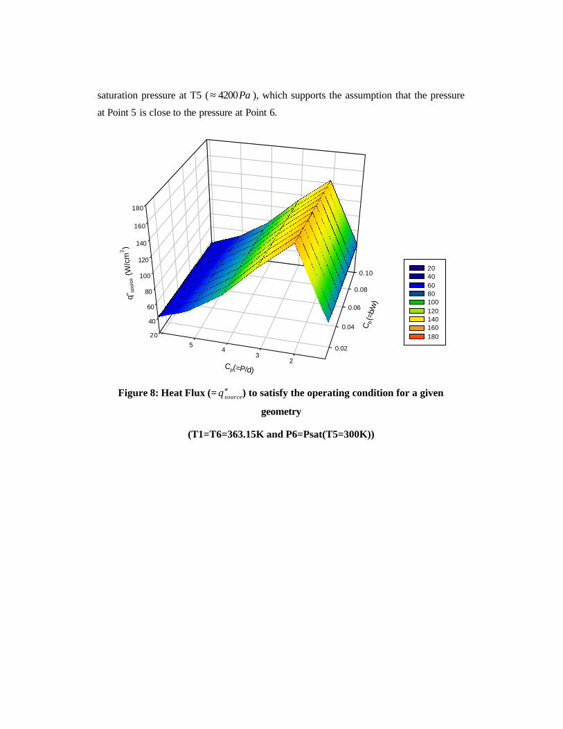
saturation pressure at T5 ( Pa4200≈ ), which supports the assumption that the pressure

at Point 5 is close to the pressure at Point 6.

20

40

60

80

100

120

140

160

180

0.02

0.04

0.06

0.08

0.10

23

45

q"so

urce

(W/c

m2)

Cb(=

b/w

)Cp(=P/d)

20 40 60 80 100 120 140 160 180

Figure 8: Heat Flux (= sourceq ′′ ) to satisfy the operating condition for a given

geometry

(T1=T6=363.15K and P6=Psat(T5=300K))

T6 (K)

320 330 340 350 360 370 380

q"so

urce

(W

/cm

2 ) or

Sou

rce

Tem

pera

ture

(K)

0

100

200

300

400

500

q"source

Source Temperature

Figure 9: Heat Flux (= sourceq ′′ ) and Heat Source Temperature for d=1.0e-5m

(Cb=0.01, Cp=2.1, P6=Psat(T5=300K)

0

5000

10000

15000

20000

25000

30000

320 340 360 380

T6 (K)

Vap

or P

ress

ure

Dro

p in

Eva

pora

tor o

rC

apill

ary

Pres

sure

(Pa)

0.0

5.0

10.0

15.0

20.0

25.0

30.0

35.0

40.0

45.0

Pres

sure

Dro

p fo

r Bot

h Li

quid

and

Vap

or in

Tra

nspo

rt L

ine

(Pa)

Total Pressure Drop

Vapor Pressure Drop inEvaporator

Capillary Pressure

Liquid Pressure Drop inPore

Liquid Pressure Drop inTransport Line

Vapor Pressure Drop inTransport Line

Figure 10: Total Pressure Drop and Capillary Pressure for d=1.0e -5m

CONCLUSION

A loop heat pipe(LHP) with coherent micron-porous evaporative w ick is suggested to

enhance the heat removal performance and it is demonstrated that this design could

achieve the high heat removal capability(>100W/cm2) with keeping the reasonable heat

source temperature(<373.15K) and satisfy the pressure limitation due to the pressure

drop. The optimized geometric parameters can be found and the maximum heat flux is

given at Cp(P/d)=2.1 and Cb(b/w)=0.01 for md 5100.1 −×= and n=10. In this paper,

there are several assumptions which may not match the real condition. The most

important things are that the temperature is uniform in evaporator. As far as our brief

estimation with computational fluid dynamics calculation, the temperature across the

evaporator varies and the evaporation rate of pores close to the conducting wall is

higher than pores far from the conducting post. Also there are some unchanged

geometric parameters such as pore diameter and number of pores in a unit cell because

these parameters are strongly related to this problem and we avoid to discuss in this

paper. In future, these things will be discussed in detail.

AKNOWLEDGEMENTS

The authors would like to acknowledge funding for this project supplied by the NASA

Commercial Space Center, Center for Space Power within the Texas Engineering

Experimental Station at Texas A&M University.

NOMENCLATURE

A Hamaker constant (J)

b width of conducting post (m)

Cp P/d

Cb b/w

d pore diameter (m)

vl DD , pipe diameter in transport line between evaporator and condenser

f friction factor

h height of conducting wall (m)

hfg latent heat (J/kg)

hv vapor enthalpy (J/kg)

k Boltzmann constant (molecule K / J)

kl thermal conductivity for working liquid (W/mK)

kwall thermal conductivity (W/mK)

l slit length (m)

M molecular weight (kg)

n number of pores per unit cell

N total number of pores in an evaporator

NA Avogadro’s number (1/mol)

P pitch between pores or slits (m)

P l bulk liquid pressure (Pa)

P li liquid pressure at interface (Pa)

P V bulk vapor pressure (Pa)

P Vi vapor pressure at interface (Pa)

evapq ′′ evaporation rate per unit horizontal pore area (W/ m2)

tatalq total thermal energy from the heat source (W)

sourceq ′′ thermal density of heat source (W/m2)

Q partial evaporation rate (W)

Q total total evaporation rate per pore or slit (W/pore )

Rgas Universal gas constant (J/kg mol K)

Rpore pore radius or half length of slit width (m)

S enthoropy (J/kgT)

Tli temperature at the interface of liquid side (K)

Tw wall temperature (K)

TV vapor temperature (K)

TVi vapor temperature at interface (K) lv specific volume of liquid (m3/kg)

V velocity (m/s)

w length per unit cell (m)

y radial coordinate (m)

z axial coordinate (m)

Γ mass flow rate (kg/m)

δ film Thickness (m)

P∆ Pressure Drop (Pa)

T∆ Temperature Difference (K)

∆z distance between nodes for axial direction

µl liquid chemical potential (J/kg/molecule) or liquid viscosity (Pa s)

µv vapor chemical potential (J/kg/molecule) or vapor viscosity (Pa s)

ν kinematic viscosity (m2/s)

Π disjoining pressure (Pa)

σ surface tension (N/m)

θ contact angle (Degree)

Superscriptions

k index of z position

line transport line between evaporator and condenser

wick wick

Subscriptions

cell unit cell

l or liq liquid

li liquid interface

p or pore pore

sat saturation condition

source heat source

v or vap vapor

vi vapor interface

w or wall wall

∞ saturation condition for flat interface

REFERENCES

1. Faghri, A, Heat Pipe Science and Technology, Washington, Taylor & Francis,

(1995).

2. Potash, M., Jr. and Wayner, P. C., Jr., “Evaporation from a Two-Dimensional

Extended Meniscus”, International Journal of Heat and Mass Transfer 15,

1851-1863 (1972).

3. DasGupta, S., Schonberg, J. A., Kim, I. Y. and Wayner, P. C., Jr., “Use of the

Augmented Young-Laplace Equation to Model Equilibrium and Evaporating

Extended Menisci”, Journal of Colloid and Interface Science 157 , 332-342 (1993).

4. Ward, C. A., Fang G., “Expression for predicting liquid evaporation flux: Statistical

rate theory approach”, Physical Review E 59, 429-440 (1999).

5. Carey, P. V., Statistical Thermodynamics and Mircoscale Thermophysics,

Cambridge(U.K.), Cambridge University Press, (1999).

6. White, M. F., Viscous Fluid Flow, New York, McGraw-Hill, Inc, (1991) .