Embed Size (px)
Citation preview

Fundamental Basics of Vacuum-energy and the Principle of the Construction of Zero-point-energy motors
Wolfenbüttel, Oktober – 21 – 2010
By Prof. Dr. Claus W. Turtur University of Applied Sciences Braunschweig-Wolfenbüttel Salzdahlumer Straße 46/48 Germany - 38302 Wolfenbüttel Tel.: (++49) 5331 / 939 - 42220 Email.: [email protected] Internet-page: http://www.ostfalia.de/cms/de/pws/turtur/FundE/index.html
PACS-classification: 84.60.-h, 89.30.-g, 98.62.En, 12.20.-m, 12.20.Ds, 12.20.Fv
Abstract The mechanism of the conversion of the zero-point-energy of the quantum-vacuum is understood. On the basis of this knowledge, it is now possible to construct zero-point-energy converters systematically. The method for this computation was developed and is presented here.
The article starts with the fundamental basics of the conversion of the zero-point-energy and explains few examples of this conversion in our everyday’s life. They are even necessary to explain the stability of matter at all.
Based on this understanding, the computation of zero-point-energy converters according to the new procedure of the „Dynamic Finite-Element-Method“ (DFEM) is explained, at first by principle, and then with the use of a concrete example for the construction of an imaginable zero-point-energy converter.
Last but not least, some thoughts regarding the philosophical background are explained, which has been necessary to make the presented development possible.
Conversion of the Zero-Point-Energy of the Vacuum, Claus W. Turtur page 2 of 52 xxx
1. Zero-point-energy in several disciplines of Physics According to our modern and generally accepted Standard-model of Astrophysics (see [Teg 02], [Rie 98], [Efs 02], [Ton 03], [Cel 07] and many others), our universe consists of - approx. 5 % well-known particles, visible matter, planets, creatures, black-holes,… - approx. 25…30 % invisible matter, such as unknown elementary-particles, - approx. 65…70 % zero-point-energy.
This statement is based on measurements of the accelerated expansion of the universe, which are based on the Doppler-shift of characteristic spectral lines of atoms in stellar and interstellar matter. However, from these measurement, the unsolved question arises, why the expansion of the universe is accelerating as function of time [Giu 00]. This experimental finding contradicts to the theoretical expectations of the Standard-model of Cosmology, according to which the expansion should slow down continuously as a function of time, because of Gravitation, which is an attractive interaction between all matter within our universe (visible matter as well as the invisible matter). And this attraction should decrease the velocity of the expansion of our universe. If we take the zero-point-energy of the vacuum into account, this question can also be solved rather easily, as we will see later in our article. (The background is the conversion of zero-point-energy into kinetic energy of the expansion of the universe.) Not only from this aspect we can see, why the disciplines of Astrophysics and Cosmology not only accept the zero-point-energy of the vacuum but they even demand its existence (see measuring-results mentioned above). And also in microscopic physics, the zero-point-energy is accepted and claimed, as for instance in Quantum Theory. Richard Feynman needs it for Quantum Electrodynamics, namely by introducing vacuum-polarization into theory. (By the way: This was the theory, which brought the author of a preceding article to his work on the zero-point-energy of the vacuum.) Vacuum-polarization describes the fact, that spontaneous virtual pair production of particle-antiparticle-pairs occurs in the empty space (i.e. in the vacuum), which annihilate after a distinct amount of time and distance (see for instance [Fey 49a], [Fey 49b], [Fey 85], [Fey 97]). Of course, these particles and anti-particles have a real mass (such as for instance electrons and positrons, resulting from electron-positron pair-production). This means, that they contain energy according to the mass-energy-equivalence ( 2E m c ). Although this matter and antimatter disappears (annihilates) soon after its creation within the range of Heisenberg's uncertainty relation, it contains energy, for which there is no other source than the empty space, from which these particles and anti-particles are created. This means that the empty space contains energy, which we nowadays call zero-point-energy. (The notation “zero-point-energy” goes back to the knowledge of its origin, which we nowadays have). It is said that this energy “from the empty space” has to disappear within Heisenberg's uncertainty relation because of the law of energy conservation. But this does not contest the fact that this energy is existing – namely as zero-point-energy of the vacuum. The energy of the empty space (vacuum-energy) should be paid more attention, and there is still much investigation to be done for its utilization. The knowledge about vacuum-polarization describes only a very small part of this vacuum-energy. Thus it is clear that vacuum-energy contains several components completely unknown up to now. Among all these components of vacuum-energy there is also this one, which we call zero-point-energy, and which describes the energy of the zero-point oscillations of the electromagnetic waves of the quantum-vacuum. This special part of the vacuum-energy has the following background: From Quantum-theory we know, that a harmonic oscillator never comes to rest. Even in the ground-state it oscillates with the given energy of ½E (see for instance [Mes 76/79], [Man 93]). This is one of the fundamental findings of Quantum-theory, which is of course

Conversion of the Zero-Point-Energy of the Vacuum, Claus W. Turtur page 3 of 52 xxx
valid also for electromagnetic waves. The consequence is that the quantum-vacuum is full of electromagnetic waves, by which we are permanently surrounded. If this concept is sensible, it should be possible to verify the existence of these zero-point-waves, for instance by extracting some of their energy from the vacuum. If it would be different, Quantum-theory would be erroneous. But in reality Quantum-theory is correct and its conception is sensible. Historically the first verification for the extraction of zero-point-energy from the quantum-vacuum comes from the Casimir-effect. Hendrik Brugt Gerhard Casimir published his theoretical considerations in 1948, suggesting an experiment with two parallel metallic plates without any electrical charge. The energy of the electromagnetic zero-point-waves should cause an attractive force between those both plates, which he calculated quantitatively on the basis of the spectrum of these zero-point-waves [Cas 48]. Because of experimental reasons (the metallic plates have to be mounted very close to each other, and the force is very small), the experimental verification of his theory was very difficult ([Der 56], [Lif 56], [Spa 58]). Thus Casimir was not taken serious for a rather long time, although his verification of the zero-point-energy is not less than a test of quantum-theory at all. Only in 1997, this is nearly half a century after Casimir’s theoretical publication, Steve Lamoreaux from Yale University [Lam 97] was able to verify the Casimir-forces with a precision of ±5%. Since this result, Casimir is taken serious and his Casimir-effect is accepted generally. Before the Lamoreaux-verification, the scientific community ignored the discrepancies between zero-point-energy and Quantum-theory simply without comment. Only since Lamoreaux’s measurement, the scientific community understood that Casimir solves many problems and he answers many open questions between vacuum-energy and Quantum-theory. Since 1997, the existence of vacuum-energy is verified not only in astrophysics, but also in a terrestric laboratory. And since this time, vacuum-energy is accepted by the scientific community. Only few years later, the industrial production of semiconductor circuits for microelectronics applications needed to take the Casimir-forces into account, in order to control the practical production of their miniaturized products. Although the research field of vacuum-energy as well as its sub-discipline of zero-point-energy (of the electromagnetic waves of the quantum-vacuum) is a very young, the scientific work in this area is very urgent because of its extremely important applications. The point is that this research field opens the door for utilization of this absolutely clean energy, which can be used as a source of energy, free from any environmental pollution. And moreover, this source of energy is inexhaustible, because it is as large as the universe itself. Mankind will have to use this energy soon, if we want to keep our planet as our habitat. The possibility to utilize this vacuum-energy is already theoretically established and also experimentally verified [Tur 09]. But the experiment could only produce a machine power of 150 NanoWatts. This is really not very much, but it is enough for a principal proof of the fundamental scientific discovery. Thus this work, done in 2009 not yet presents a technical engine, but only the basic scientific verification of the zero-point-energy of the vacuum. Consequently it should be expected, that the next step now will be to build prototypes of this engine for practical engineering techniques with larger machine power. Nevertheless, there is a better way to process, namely as following. If we look into the available literature, we find that there is already an amazingly large number of existing approaches, to convert vacuum-energy into some classical type of energy. A good overview about the work already available can be found at the book [Jeb 06]. There we read, that successful work is done by laymen as well as by honourable institutes such as Massachusetts Institute of Technology (MIT). Some work is even done by military and secret
Conversion of the Zero-Point-Energy of the Vacuum, Claus W. Turtur page 4 of 52 xxx
services ([Hur 40], [Nie 83], [Mie 84]). If we dedicate our attention to available reports, we immediately see, that there are already existing zero-point-energy-converters with a machine power of many orders of magnitudes larger than mine with only 150 NanoWatts. Obviously mankind already managed to take zero-point-energy converters into operation, with handy dimensions and a machine-power of several Watts or sometimes even several KiloWatts. Even if the utilization of the clean, pollution-free and inexhaustible vacuum-energy is not yet known by everybody, because the intellectual hurdle for its discovery is rather high, it is already clear that this is the energy technology of the upcoming third millennium. It will gain the energy-market within a foreseeable number of years, because mankind needs it to survive [Sch 10], [Ruz 09]. And it will bring a new industrial boom, because all the energy-consuming industry will have enough energy without limitation, as well as private people will have. Similar as the reduction of the prices of semiconductors increased the business of semiconductor-industry, the reduction of the prices of energy will increased the business also of the energy-producing industry. We can be glad about all these practical engineers, who construct vacuum-energy-converters from their intuition, because they help us to find our way towards clean energy. Nevertheless we face the necessity to develop a proper physical theory for the understanding of such converters. The necessary scientific work will not only give us the possibility to understand the fundamental basics of zero-point-energy and its conversion into classical energy, but it would also give us the possibility to perform a systematic construction and optimization of such engines. A contribution to this scientific knowledge was developed by the author of the preceding article in [Tur 09]. But the article here presents the understanding of the principles of zero-point-energy conversion in a way, that it will be possible to develop method to calculate zero-point-energy converters in a way, that the systematic technical construction of these engines will be possible in not too far future.
2. The Energy-circulation of the Fields of the Interactions We begin our considerations with a remembrance of the energy-circulation of the electric and the magnetic fields, which is described in [Tur 07a] und [Tur 07b]: As we know, every electric charge emits an electric field, of which the field-strength can be determined by Coulomb’s law [Jac 81]. This field contains field energy, which can be determined from the field-strength. The field-strength of the electric is
30
1
4π
QE r r
r
with Q electrical charge, r
distance from the charge, 12
0 8.854187817 10 A sV m electrical field-constant [Cod 00].
(1)
The energy density is determined as
2 220 02 2 4
0 0
1
2 2 4π 32π
Q Qu E
r r
. (2)
We know that the field contains energy, depending (among others also) on the amount of space, which is filled by the field. Furthermore we know from the Theory of Relativity as well as from the mechanism of the Hertz’ian dipole-emitter, that electric fields (same as magnetic fields, AC-fields as well as DC-fields) propagate with the speed of light (see [Goe 96], [Pau 00], [Sch 02], and others). Thus every electric charge as the source of the field permanently emits field-energy. This is a feature of the field-source and the field. (The property to be a field source is calculated mathematically by the use of the Nabla-operator, as written for instance in Maxwell's equations.)
Conversion of the Zero-Point-Energy of the Vacuum, Claus W. Turtur page 5 of 52 xxx
But from where does the charge (being the field-source) receive its energy, so that it can permanently provide the field energy ?
The answer again goes back to the vacuum-energy, namely to the above mentioned energy-circulation: On the one hand, every charge in the empty space is supported permanently with energy, and because this is also the case if the charge is only in contact with the empty space (the vacuum), the energy can only be provided by the vacuum. On the other hand, the field gives a certain amount of energy during its propagation through the empty space back to the vacuum. This conception was developed in [Tur 07a] and it was proven in [Tur 07b]. This means that the charge converts vacuum-energy into field-energy, and the field gives back this energy to the vacuum, during its propagation into the space. This is the energy-circulation mentioned above. The functioning-mechanism behind this type of “back and forth” energy-conversion (circulation) is not yet completely clarified. It should be mentioned that this type of energy-circulation is recognized not only for the electric field, but also for the magnetic field. This is also theoretically proven in [Tur 09]. Furthermore, the electromagnetic interaction is not the only one in nature, which can be described by an appropriate potential (a scalar-potential or a vector-potential A
).
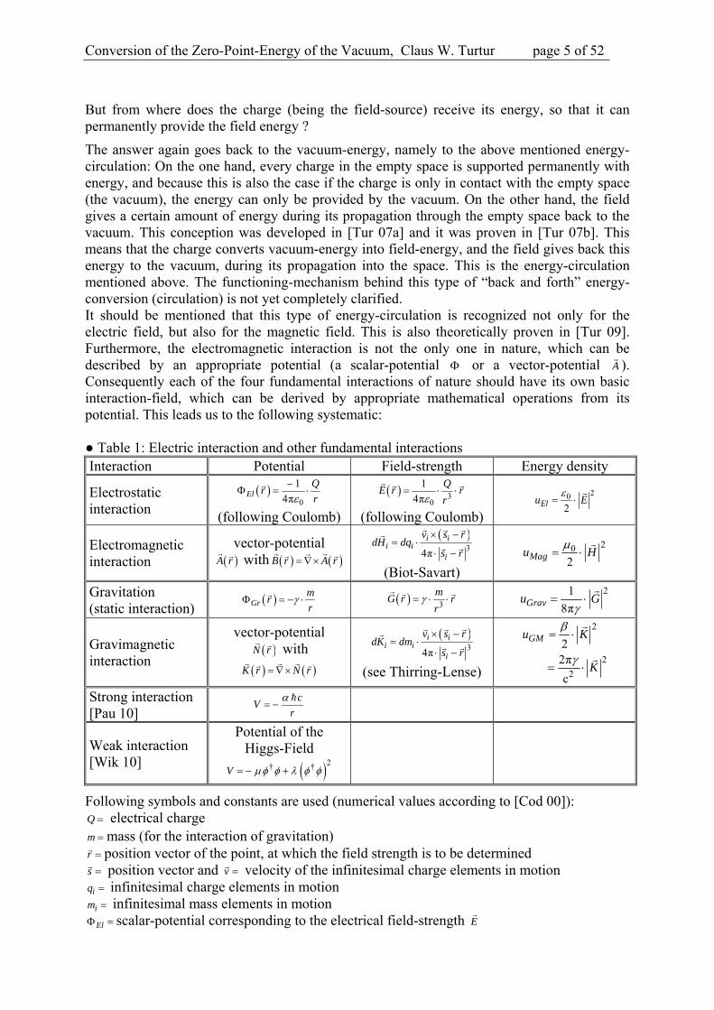
Consequently each of the four fundamental interactions of nature should have its own basic interaction-field, which can be derived by appropriate mathematical operations from its potential. This leads us to the following systematic: ● Table 1: Electric interaction and other fundamental interactions Interaction Potential Field-strength Energy density
Electrostatic interaction
0
1
4πElQ
rr
(following Coulomb)
30
1
4π
QE r r
r
(following Coulomb)
20
2Elu E
Electromagnetic interaction
vector-potential A r with B r A r
3
4π
i ii i
i
v s rdH dq
s r
(Biot-Savart)
20
2Magu H
Gravitation (static interaction)
Grm
rr
3
mG r r
r
21
8πGravu G
Gravimagnetic interaction
vector-potential N r with
K r N r
3
4π
i ii i
i
v s rdK dm
s r
(see Thirring-Lense)
2
2
2
22π
c
GMu K
K
Strong interaction [Pau 10]
cV
r
Weak interaction [Wik 10]
Potential of the Higgs-Field
2† †V
Following symbols and constants are used (numerical values according to [Cod 00]): Q electrical charge m mass (for the interaction of gravitation) r position vector of the point, at which the field strength is to be determined s position vector and v
velocity of the infinitesimal charge elements in motion iq infinitesimal charge elements in motion im infinitesimal mass elements in motion El scalar-potential corresponding to the electrical field-strength E
Conversion of the Zero-Point-Energy of the Vacuum, Claus W. Turtur page 6 of 52 xxx
Gr scalar-potential corresponding to the gravitational field-strength G
iH dH
electromagnetic field-strength
iK dK
gravimagnetic field-strength
electrical field-constant: 2
92
0
18.987551788 10
4π
N m
C
(weil 120 8.854187817 10
A s
V m
)
magnetic field-constant: 2
70 2
4π 10N s
C
. It is: 0
00 0 2 1 2
4π
1 4π
cc
gravitational field-constant: 2
112
6.6742 10N m
kg
gravimagnetic field-constant: 2
272 2
4π9.3255 10
c
N s
kg It is:
2
4π
c
It should be mentioned that there are several possible descriptions of the fundamental interactions (besides this one given here) within the theory. The most widespread alternative description uses exchange particles – for each fundamental interaction an individual type of exchange particles. (For further details, please see section 6 of the present article.) We now want to calculate, how much power (energy per time) the field-source of the electric field (i.e. the electric charge) respectively the field source of the gravitational fields (i.e. the ponderable mass) emits. ● As an example for the first mentioned interaction, we regard the electron as a source of the electric field, and thus we begin our calculation with the energy density of the electric field at the surface of the electron:
22 290 0
2 30
11.45578 10
2 2 4πEle
Q Ju E
R m
(3)
For the determination of the numerical value of the field strength at the surface of the electron, that classical electron’s radius of 152.818 10ER m (according to [COD 00]) was used. When the field-energy is flowing out of the electron with this energy-density (and with the speed of light), we can calculate the amount of energy per time, which passes an infinitesimal thin spherical shell on the surface of the electron. This is the amount of energy being emitted by the electron. For this calculation, let s be the thickness of this spherical shell and c be the speed of light, with which the field flows through the shell. Then a given field-element will
pass the shell within the time xs
tc
. Thus, the amount of energy being emitted with the time-
interval xt is El ElW u s A . This is the amount of energy, which passes the electron’s surface A within the time-interval xt .
This leads to an emitted power of El ElEl El
xsc
W u s AP u A c
t
(4)
Putting the electron’s surface 24π EA R into this expression, and further using (3), we derive
2 22 90
2 2 4 2 20 0
4π 4.355 102 sec.16π 8π
El El Ee e
Q c Q JouleP u A c R c
R R
(5)
This is a tremenduously large power with regard to this very tiny particle of a single electron. This means that every electron emits GigaWatts. In order to illustrate this amount of energy
Conversion of the Zero-Point-Energy of the Vacuum, Claus W. Turtur page 7 of 52 xxx
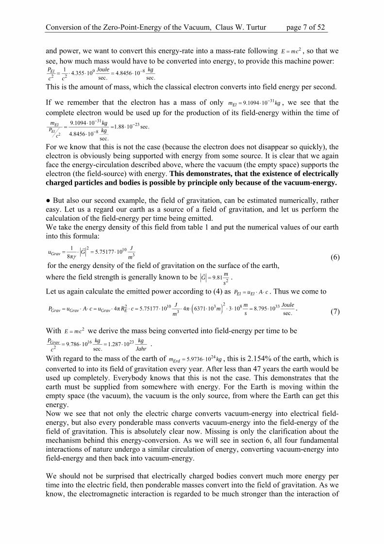
and power, we want to convert this energy-rate into a mass-rate following 2E mc , so that we see, how much mass would have to be converted into energy, to provide this machine power:
9 82 2
14.355 10 4.8456 10
sec. sec.ElP Joule kg
c c
This is the amount of mass, which the classical electron converts into field energy per second.
If we remember that the electron has a mass of only 319.1094 10Elm kg , we see that the complete electron would be used up for the production of its field-energy within the time of
2
3123
8
9.1094 101.88 10 sec.
4.8456 10sec.
El
ElP
c
m kgkg
For we know that this is not the case (because the electron does not disappear so quickly), the electron is obviously being supported with energy from some source. It is clear that we again face the energy-circulation described above, where the vacuum (the empty space) supports the electron (the field-source) with energy. This demonstrates, that the existence of electrically charged particles and bodies is possible by principle only because of the vacuum-energy. ● But also our second example, the field of gravitation, can be estimated numerically, rather easy. Let us a regard our earth as a source of a field of gravitation, and let us perform the calculation of the field-energy per time being emitted. We take the energy density of this field from table 1 and put the numerical values of our earth into this formula:
2 103
15.75177 10
8πGravJ
u Gm
for the energy density of the field of gravitation on the surface of the earth, (6)
where the field strength is generally known to be 2
9.81m
Gs
.
Let us again calculate the emitted power according to (4) as El ElP u A c . Thus we come to
22 10 3 8 333
4π 5.75177 10 4π 6371 10 3 10 8.795 10sec.Grav Grav Grav E
J m JouleP u A c u R c m
sm . (7)
With 2E mc we derive the mass being converted into field-energy per time to be 16 23
29.786 10 1.287 10
sec.GravP kg kg
Jahrc .
With regard to the mass of the earth of 245.9736 10Erdm kg , this is 2.154% of the earth, which is converted to into its field of gravitation every year. After less than 47 years the earth would be used up completely. Everybody knows that this is not the case. This demonstrates that the earth must be supplied from somewhere with energy. For the Earth is moving within the empty space (the vacuum), the vacuum is the only source, from where the Earth can get this energy. Now we see that not only the electric charge converts vacuum-energy into electrical field-energy, but also every ponderable mass converts vacuum-energy into the field-energy of the field of gravitation. This is absolutely clear now. Missing is only the clarification about the mechanism behind this energy-conversion. As we will see in section 6, all four fundamental interactions of nature undergo a similar circulation of energy, converting vacuum-energy into field-energy and then back into vacuum-energy. We should not be surprised that electrically charged bodies convert much more energy per time into the electric field, then ponderable masses convert into the field of gravitation. As we know, the electromagnetic interaction is regarded to be much stronger than the interaction of
Conversion of the Zero-Point-Energy of the Vacuum, Claus W. Turtur page 8 of 52 xxx
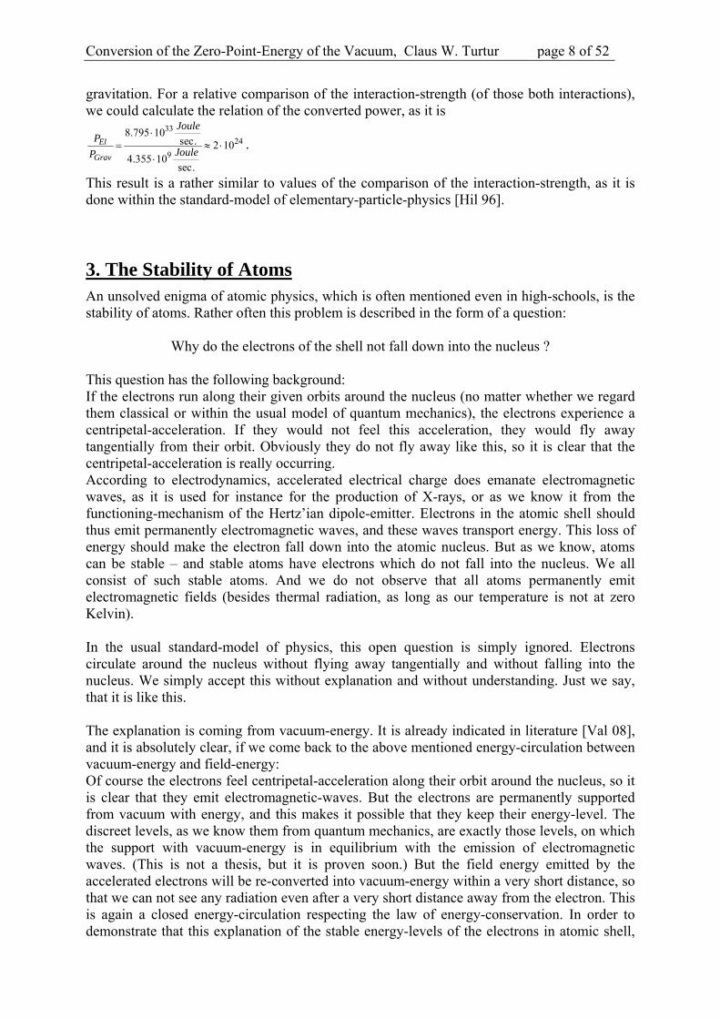
gravitation. For a relative comparison of the interaction-strength (of those both interactions), we could calculate the relation of the converted power, as it is
33
24
9
8.795 10sec. 2 10
4.355 10sec.
El
Grav
JouleP
JouleP
.
This result is a rather similar to values of the comparison of the interaction-strength, as it is done within the standard-model of elementary-particle-physics [Hil 96].
3. The Stability of Atoms An unsolved enigma of atomic physics, which is often mentioned even in high-schools, is the stability of atoms. Rather often this problem is described in the form of a question:
Why do the electrons of the shell not fall down into the nucleus ? This question has the following background: If the electrons run along their given orbits around the nucleus (no matter whether we regard them classical or within the usual model of quantum mechanics), the electrons experience a centripetal-acceleration. If they would not feel this acceleration, they would fly away tangentially from their orbit. Obviously they do not fly away like this, so it is clear that the centripetal-acceleration is really occurring. According to electrodynamics, accelerated electrical charge does emanate electromagnetic waves, as it is used for instance for the production of X-rays, or as we know it from the functioning-mechanism of the Hertz’ian dipole-emitter. Electrons in the atomic shell should thus emit permanently electromagnetic waves, and these waves transport energy. This loss of energy should make the electron fall down into the atomic nucleus. But as we know, atoms can be stable – and stable atoms have electrons which do not fall into the nucleus. We all consist of such stable atoms. And we do not observe that all atoms permanently emit electromagnetic fields (besides thermal radiation, as long as our temperature is not at zero Kelvin). In the usual standard-model of physics, this open question is simply ignored. Electrons circulate around the nucleus without flying away tangentially and without falling into the nucleus. We simply accept this without explanation and without understanding. Just we say, that it is like this. The explanation is coming from vacuum-energy. It is already indicated in literature [Val 08], and it is absolutely clear, if we come back to the above mentioned energy-circulation between vacuum-energy and field-energy: Of course the electrons feel centripetal-acceleration along their orbit around the nucleus, so it is clear that they emit electromagnetic-waves. But the electrons are permanently supported from vacuum with energy, and this makes it possible that they keep their energy-level. The discreet levels, as we know them from quantum mechanics, are exactly those levels, on which the support with vacuum-energy is in equilibrium with the emission of electromagnetic waves. (This is not a thesis, but it is proven soon.) But the field energy emitted by the accelerated electrons will be re-converted into vacuum-energy within a very short distance, so that we can not see any radiation even after a very short distance away from the electron. This is again a closed energy-circulation respecting the law of energy-conservation. In order to demonstrate that this explanation of the stable energy-levels of the electrons in atomic shell,
Conversion of the Zero-Point-Energy of the Vacuum, Claus W. Turtur page 9 of 52 xxx
which is an alternative to the explanation of quantum theory, is not some strange or grotesque train of thoughts, it must be mentioned, that there is the theory of Stochastic Electrodynamics, with many publications in highly respected physic’s journals, which uses exactly this alternative train of thoughts as a basis for the calculation of all well-known results of Quantum-mechanics, without using any formalism of Quantum-mechanics at all (for a long list of literature please see [Boy 66..08], but also see the information at [Boy 80], [Boy 85]). A respected scientific group (Calphysics Institute) does remarkable work in the field of the vacuum-energy on the basis of Stochastic Electrodynamics and the support of circulating electrons with zero-point-energy [Cal 84..06]. (This is one of several aspects of their work.) The only basic assumption of the theory of Stochastic Electrodynamics is the postulate, that the zero-point-oscillations of electromagnetic waves exist (although these waves have been originally discovered within Quantum-theory). Within Stochastic Electrodynamics, the spectrum of these zero-point-waves define the ground state of the electromagnetic radiation of the empty space, this is the vacuum-level. From their interactions with the electrons in the atomic shell, the energy-levels of the electrons are determined. Further assumptions of Quantum-theory are not necessary within Stochastic Electrodynamics.
If we regard the interaction between these zero-point-waves (of the vacuum) and the matter in our world, we see that all particles of matter absorb and re-emit such waves, because all elementary particles permanently carry out zero-point-oscillations. On the basis of this conception, Stochastic Electrodynamics is capable to derive all phenomena, which we know from Quantum-theory, without using Quantum-theory at all.
Historically the first result of Stochastic Electrodynamics was: The black body radiation with its characteristic spectrum as a function of temperature results from the movement of the elementary-particles of which the body consists, and which perform zero-point oscillations. The next result of Stochastic Electrodynamics was the photo-effect. In the history of Quantum-mechanics, one of the prominent results was the explanation of the energy levels of the electrons in atomic shell. In the formalism of Stochastic Electrodynamics, stable states (at which electrons can stay) are achieved when the energy being emitted from the electrons because of their circulation around the nucleus, is identically compensated by the energy which they absorb from the zero-point radiation of the vacuum. (This contains an explanation, why the electrons do not fall into the nucleus because they lose energy due to their circulation. There is some analogy with Bohr’s first and third postulate, according to which stable states of shell-electrons are only possible for constructive interference of the electron-waves.) And finally it should be said, that the equilibrium between absorbed and emitted radiation (in Stochastic Electrodynamics) leads to the same discrete energy-levels as we know them from Quantum-mechanics.
Not only the results of Quantum-mechanics but also the results of Quantum-Electrodynamics are reproduced with the formalism of Stochastic Electrodynamics, for instance such as the Casimir-effect, van der Waals- forces, the uncertainty principle (which has been derived the first time by Heisenberg) and many others.
For the sake of completeness it should be remarked, that Stochastic Electrodynamics of course explains the phenomena of nature on its own, not trying to reproduce the mathematical structure of Quantum-theory and even not in connection with the formalism of Quantum-theory. So for example the famous Schrödinger-equation, as a typical formula of Quantum-theory can not be derived with the means of Stochastic Electrodynamics, because such a formula simple is not a topic of Stochastic Electrodynamics. In the same way, formulas of Stochastic Electrodynamics can not derived within Quantum-theory. In this sense, Stochastic
Conversion of the Zero-Point-Energy of the Vacuum, Claus W. Turtur page 10 of 52 xxx
Electrodynamics and Quantum-theory are two independent concepts, which describe the same phenomena of nature, but which have totally different philosophical background.
It is known that Stochastic Electrodynamics is not as widespread as Quantum-theory. But it is in complete confirmation with all nowadays known phenomena of nature. Thus it is sensible to accept it for further considerations of “how to extract energy from the zero-point-oscillations”, which can lead to interesting results, because new thoughts might emerge. The zero-point-oscillations and the zero-point-waves are the central fundament of Stochastic Electrodynamics.
In this sense, we could describe the relationship between Stochastic Electrodynamics and Quantum Mechanics a little bit provocative, but with logical consequence: The fundamental of phenomenon of nature, which is described by both theories, is the existence of the electromagnetic zero-point-waves in the vacuum, which we see as a part of the whole vacuum-energy. On the basis of these waves, it is possible to establish two different mathematical formalisms, independently of each other. One formalism is known as Stochastic Electrodynamics and the other one as Quantum Mechanics. Both of them have the same capability to explain the phenomena of nature. Both of them accept and the need vacuum-energy. Vacuum-energy is the only common feature of both theories. Thus vacuum-energy is to be regarded as the real fundament. Both theories are mathematical structures, which use vacuum-energy and draw their conclusions from it. Stochastic Electrodynamics is explicitly conscious of this fact, whereas Quantum Mechanics has this consciousness only implicitly somewhere in background. Because Quantum Theory would not work without vacuum-energy, it is also based on vacuum-energy. This is the moment for a short intermediate recapitulation of the sections 1-3:
1. The dominant part of our universe is vacuum-energy (even if we don't see it directly). 2. Physical entities as we know them from everyday’s life, such as electrical charges and
ponderable masses, can only exist because of vacuum energy. Vacuum-energy is the fundament of all interactions between all particles which we know.
3. Also the existence of atoms is only possible because of vacuum-energy, and the theory of atoms is based finally on vacuum-energy.
4. A fundamental understanding of the term “field”
In [Tur 08] the author of this article presented the following explanation for electrical (as well as magnetic) fields, which shall be recapitulated in short terms here: The empty space (i.e. the vacuum) contains zero-point-waves. They have their continuous spectrum of wavelengths inside the space without field. But if a field is applied, the wave-lengths are reduced in comparison to the wavelengths without field. The fundament of this conception is a work done by Heisenberg and Euler, in which they develop the Lagrangeian of electromagnetic waves within electric and magnetic fields, and they analyze the influence of the fields on the speed of propagation of those waves [Hei 36]. They come to the result, that the speed of light in space containing field is slower, than the speed of light in the space without field. (The latter one is the vacuum speed of light as being used in the Theory of Relativity.) This old work by Heisenberg has been confirmed and further developed by [Bia 70] and by [Boe 07], who quantitatively calculate the reduction of the speed of propagation of electromagnetic waves as a function of the applied field strength.
From there we know, that the speed of electromagnetic waves is reduced by electric and magnetic DC-fields, and we postulate that also the waves in the ground-state (i.e. the zero-
Conversion of the Zero-Point-Energy of the Vacuum, Claus W. Turtur page 11 of 52 xxx
point-waves) follow this behaviour. The feature to reduce the speed of waves is a feature of the fields themselves.
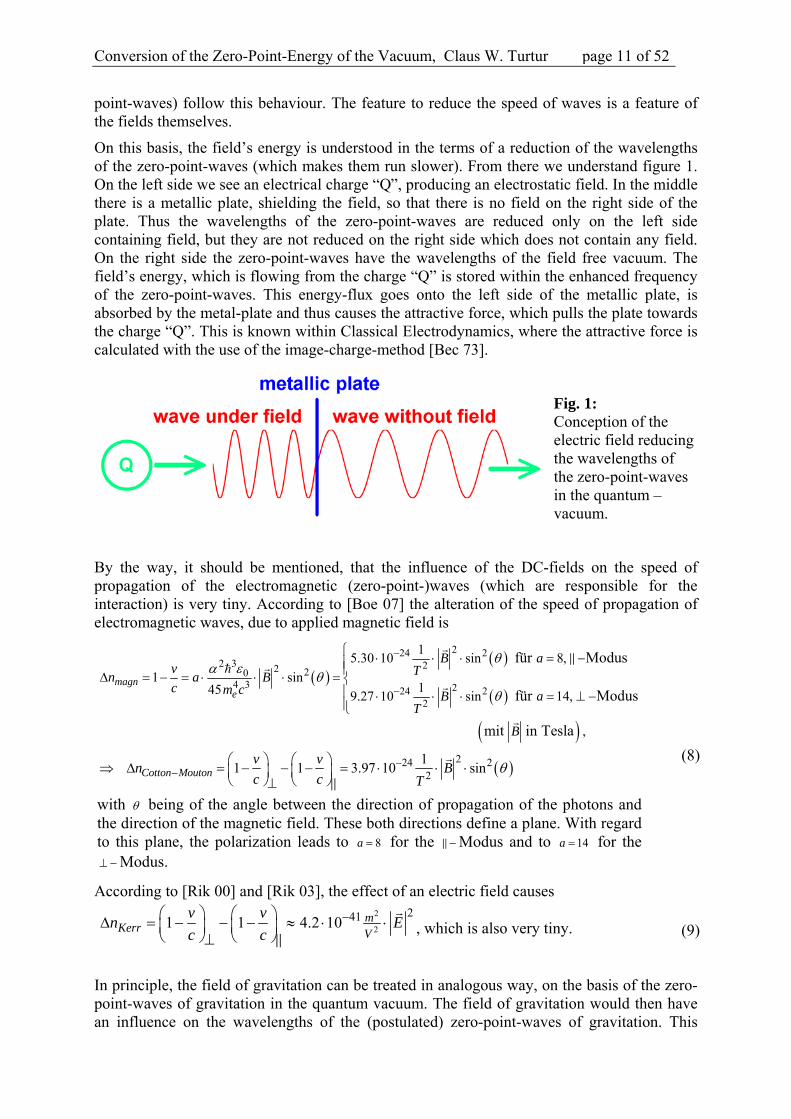
On this basis, the field’s energy is understood in the terms of a reduction of the wavelengths of the zero-point-waves (which makes them run slower). From there we understand figure 1. On the left side we see an electrical charge “Q”, producing an electrostatic field. In the middle there is a metallic plate, shielding the field, so that there is no field on the right side of the plate. Thus the wavelengths of the zero-point-waves are reduced only on the left side containing field, but they are not reduced on the right side which does not contain any field. On the right side the zero-point-waves have the wavelengths of the field free vacuum. The field’s energy, which is flowing from the charge “Q” is stored within the enhanced frequency of the zero-point-waves. This energy-flux goes onto the left side of the metallic plate, is absorbed by the metal-plate and thus causes the attractive force, which pulls the plate towards the charge “Q”. This is known within Classical Electrodynamics, where the attractive force is calculated with the use of the image-charge-method [Bec 73].
Fig. 1: Conception of the electric field reducing the wavelengths of the zero-point-waves in the quantum –vacuum.
By the way, it should be mentioned, that the influence of the DC-fields on the speed of propagation of the electromagnetic (zero-point-)waves (which are responsible for the interaction) is very tiny. According to [Boe 07] the alteration of the speed of propagation of electromagnetic waves, due to applied magnetic field is
224 22 3 22 20
4 3 224 22
15.30 10 sin 8,
1 sin145 9.27 10 sin 14,
,
für Modus
für Modus
mit in Tesla
magne
B av Tn a Bc m c B a
T
B
224 22
11 1 3.97 10 sinCotton Mouton
v vn B
c c T
with being of the angle between the direction of propagation of the photons and the direction of the magnetic field. These both directions define a plane. With regard to this plane, the polarization leads to 8a for the Modus and to 14a for the Modus.
(8)
According to [Rik 00] and [Rik 03], the effect of an electric field causes 2
2
2411 1 4.2 10 mKerr V
v vn E
c c
, which is also very tiny. (9)
In principle, the field of gravitation can be treated in analogous way, on the basis of the zero-point-waves of gravitation in the quantum vacuum. The field of gravitation would then have an influence on the wavelengths of the (postulated) zero-point-waves of gravitation. This

Conversion of the Zero-Point-Energy of the Vacuum, Claus W. Turtur page 12 of 52 xxx
conception of “fields reducing the zero-point-waves of their individual interaction” can be applied to all fundamental interactions in physics, as we will discuss in section 6. The only exception is the Strong interaction, which can not be transferred directly one by one into this model. But this is not the large problem, because the Strong interaction is said to be not completely understood in the Standard model of elementary particle physics (see section 6).
What I also want to mention, is the difference between static fields (such as the electrostatic field and static field of gravitation) and magnetic fields (such as the electromagnetic field and the gravimagnetic field). The existence of the electromagnetic field is generally known. The existence of the gravimagnetic field, is also known by theory [Thi 18] and verified experimentally [Gpb 07], but the knowledge is not widespread among everybody. In history of physics it was derived from the Theory of General Relativity.
The question is now: Static fields reduce the wavelength of the zero-point-waves, but magnetic fields do something very similar. There is a difference between the effects of those both types of fields, the static and the magnetic fields. How can we understand this ?
The answer is surprisingly simple: The difference is a coordinate-transformation, namely the Lorentz-transformation. If an observer is in rest with regard to the field source (for instance an electric charge) the observer will only see the static field. But if the observer is moving with regard to the field source, he will additionally see an electric current (due to the motion of the electric charge), and he will have to calculate additionally the magnetic field produced by this current. This calculation can be done on the one hand by the classical formulas for magnetic fields within classical Electrodynamics, but on the other hand this calculation can be done by taking the relativistic length-contraction of the wavelengths of the zero-point-waves (due to the movement) into account [Dob 03]. Both ways of calculation lead to the same force of interaction and to the same field’s energy.
With regard to our concept of the reduced wavelengths of the zero-point-waves, this means: If an observer is moving relatively to the field source, relativistic length-contraction additionally reduces the wavelength of the zero-point-waves. And this additional reduction can be described in terms of a magnetic field.
But now, please focus your attention to the finite speed of propagation of the zero-point-waves, and to the alteration of this speed of propagation due to an applied DC-field. An illustration for a further very important aspect is to be found in figure 2:
Let us start our considerations with the very first line on top of this figure. There we see a sphere on the left side of the drawing, which is drawn with green colour. The sphere does not carry any electrical charge in the first line. The electromagnetic zero-point-waves of the quantum vacuum (in red colour) are flowing without any influence of any field. They propagate with the vacuum speed of light, such as they always do it in the space without any field.
The time is represented in steps from line to line with increasing time from the top to the bottom.
In the next (second) line of figure 2, an electrical charge “Q” is brought onto the green sphere. This causes a reduction of the wavelengths of the electromagnetic zero-point-waves which come into the electrostatic field. They also propagate into the space. But they (i.e. the “blue waves”) are propagating a little bit slower than the “red” waves. This difference of speed of propagation causes a small gap between the “blue” and the “red” wave trains.
As long as the electrical charge “Q” is present on the green sphere, the electromagnetic zero-point-waves will propagate with the reduced wavelength, as we see it also in line number 3.
Conversion of the Zero-Point-Energy of the Vacuum, Claus W. Turtur page 13 of 52 xxx
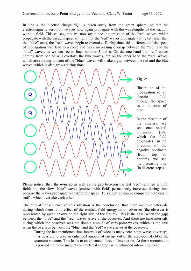
In line 4 the electric charge “Q” is taken away from the green sphere, so that the electromagnetic zero-point-waves now again propagate with the wavelengths of the vacuum without field. This causes, that we now again see the emission of the “red” waves, which propagate with the vacuum speed of light. For the “red” waves propagate a little bit faster than the “blue” ones, the “red” waves begin to overtake. During time, this difference of the speed of propagation will lead to a more and more increasing overlap between the “red” and the “blue” waves, as we can see in lines number 5 and 6. On the one hand the “red” waves coming from behind will overtake the blue waves, but on the other hand the “red” waves, which are running in front of the “blue” waves will make a gap between the red and the blue waves, which is also grows during time.
Fig. 2: Illustration of the propagation of an electric field through the space as a function of time. In the direction of the abscissa, we see one spatial dimension (into which the field propagates), in the direction of the negative oordinate (from top to bottom), we see the increasing time (in discrete steps).
Please notice, then the overlap as well as the gap between the fast “red” (emitted without field) and the slow “blue” waves (emitted with field) permanently increases during time, because the waves propagate with different speed. This situation can be compared with cars in traffic which overtake each other.
The crucial consequence of this situation is the conclusion, that there are time intervals, during which there is no effect of the emitted field-energy on an observer (the observer is represented by green arrows on the right side of the figure). This is the case, when the gaps between the “blue” and the “red” waves arrive at the observer. And there are time intervals, during which the observer sees the double amount of zero-point-waves, which is the case when the overlaps between the “blue” and the “red” wave arrives at the observer.
- During the last mentioned time-intervals of twice as many zero-point-waves (overlap), it is possible to take an enhanced amount of energy out of the zero-point-field of the quantum vacuum. This leads to an enhanced force of interaction. At these moments, it is possible to move magnets or electrical charges with enhanced interacting force.

Conversion of the Zero-Point-Energy of the Vacuum, Claus W. Turtur page 14 of 52 xxx
- During the first mentioned time-intervals of the gaps, there is no field-force acting on the observer. At these moments, it is possible to move magnets or electrical charges without any interacting force.
This should open the way to a practical utilization of the zero-point-waves for the conversion of vacuum energy – as soon as we will be able, to build a machine, which always does the right type of movement in the right (appropriate) moment. And example for this mechanism could be the following:
■ During the phase of the overlap of the zero-point-waves (simultaneous arrival of both waves), we allow the parts of the machine converting vacuum-energy to follow the Coulomb-force (or magnetic force), so that the force is an enhanced because of the overlap. In the case of an attractive force, the parts of the engine should move towards each other. This very special movement gains more energy, then we can expect from the simplified laws of classical Electrodynamics, which do not take the finite speed of propagation of the fields into account.
■ During the phase of the gap between the zero-point-waves (missing interaction-force within the gap) we have to perform the opposite direction of the movement of the parts of the machine converting vacuum-energy, this is the direction against the Coulomb-force (or magnetic force). In the case of an attractive force, the parts of the engine should move away from each other. During this very special movement, the distance between attractive parts of the machine can be enhanced without a force – different then we can expect from the simplified laws of Electrodynamics, which do not take the finite speed of propagation of the fields into account.
By this means it must be possible, to construct closed cycles of movement, along which the attractive direction gains more energy than the repulsive direction consumes.
This explanation describes the fundamental principle, according to which electric and magnetic vacuum-energy-converters can operate.
Up to now, several inventors are known, who constructed vacuum-energy converts by intuition, finding an functioning machine by „trial and error“. But none of them has a clear idea about the theoretical working-principle behind his machine. And none of them is capable to optimize his machine systematically on the basis of such a theory. They all do the optimization by „trial and error“ (and the have success nevertheless).
Many of them report about high frequency impulses, and this is not surprising, if we look to the small differences in propagation-time between the “red” and the “blue” zero-point-waves.
With the concept presented here, the fundamental functioning principle of vacuum-energy converters is found. This is the basic fundament for the construction of vacuum-energy converters at all. It is now the task to apply this knowledge and to build vacuum-energy converters on this principle, and to optimize these devices systematically.
Conversion of the Zero-Point-Energy of the Vacuum, Claus W. Turtur page 15 of 52 xxx
5. Practical methods for the construction of vacuum-energy converters In order to construct a new vacuum-energy converter, or to calculate the functioning of existing one, the following steps define a scheme of operation.
1. step: Preparation by a classical FEM-computation
The geometry of the machine and especially of its field sources (i.e. magnets or electric charges) has to be modelled with a computer. A possible instrument therefore is the method of finite elements (FEM). But a classical FEM-program can only take this model of the machine and calculate the forces between the different parts of the engine without taking the speed of propagation of the fields into account [Ans 08].
Even if the theory behind such an FEM-algorithm is called electrodynamics, we regard the computation as a static one, because the time-dependency of the propagation of the fields during the space is neglected.
For typical engines made by mankind in the laboratory or in industrial production, this simplified static Theory is absolutely sufficient, because the distances between those parts of the engine, which interact with each other, is so small, that the time for the propagation of the fields don't play a serious role. For example, if an electric engine is a smaller than one meter, the propagation-time for the magnetic fields with the speed of light is less than
81
3.3310 m
s
mv Nano Secondsst
, to propagate from one end of the engine to the opposite end. For
the practical construction of classical engines (not for zero-point-energy converters) such small time-intervals are absolutely not important. For such engines, the static Theory of classical Electrodynamics is fully sufficient. This is different from zero-point-energy converters, whose principle is based on the dynamic time-dependency of the propagation of the fields.
2. step: Supplement of a real dynamic of the field-propagation to the FEM-method
(2.a.) Practical aspects for the production: If a zero-point-energy converter shall be constructed, the principles of section 4 have to be taken into account, which are based on the finite speed of propagation of the fields. For the setup to be constructed, the time-intervals for the propagation of the fields with the speed of light, have to be dissected precisely (taking the necessary effort). This makes it necessary to build the machines in such a way, that the motions of its parts are short and fast enough, that the parts of the engine can feel the overlaps and the gaps between the “blue” and the “red” waves of figure 2. Because these gaps and overlaps depend on the speed of light, it is necessary to work with rather high speed of revolution and with rather high frequency of the signals and/or pulses as well as high frequency fields.
(2.b.) Computing method: In order to realize the described construction, it is necessary to add the real dynamics of the time-dependency of the propagation of the fields to the Finite-Element-Method. Thus it is not enough to register all positions of all components of the machine as it was done under (2.a.), But it is additionally necessary to register fully all components of the machine with their complete motion in space and time. This means: In addition to the three spatial dimensions of the static Theory of classical Electrodynamics, we now have to add the dimension of time. And there is even more additional work to be done: This is necessary not only for all
Conversion of the Zero-Point-Energy of the Vacuum, Claus W. Turtur page 16 of 52 xxx
mechanical and electromagnetic components of the machine, but also (and this is very important) for all fields of interaction, which have to be treated as individual parts of the machine. The propagation of these fields must be taken into account, same as the motion of all other parts of the engine. Every hardware component of the machine emits a field during the consecutive time 1t , and this field starts its propagation at the position 1 1 1 1, ,x y zr , from
where it is emitted at the time 1t . And from this moment on, the field propagates all over the machine, so that it will reach an other component of the machine at the time 2t at the position
2 2 2 2, ,x y zr . And there it will cause a force of interaction (independently from the question,
to which position the field-emitting hardware has been moving in the meantime). For the operation of the engine, the motion of all of its active components as a function of time 1t …
2t has to be taken into account, so that we know their positions
1 1 1 1, ,t x t y t z tr and 2 2 2 2, ,t x t y t z tr
, … , ,n n n nt x t y t z tr ,
where the machine consists of n components. But additionally the dynamic-FEM simulation (DFEM) on the computer needs the behaviour of all fields of interaction in the same way, these are the data
1 , , ,x y z tE
, 2 , , ,x y z tE
, …, , , ,k x y z tE
for the dynamic propagation of the electric fields, and
1 , , ,x y z tB
, 2 , , ,x y z tB
, …, , , ,k x y z tB
for the dynamic propagation of the magnetic fields.
Only if the motion of all hardware components of the machine during space and time, and the motion of all fields during space and time is completely included into the simulation, the computation of a vacuum-energy-converter is possible. This condition is absolutely necessary, because the finite speed of propagation of the fields and the alteration of the speed of propagation of the zero-point-waves is the basis of the conversion of vacuum-energy. Only if we take the time of the propagation-speed of the zero-point-waves into account, we are capable to extract energy from these waves.
In view of the DFEM-computation, the most uncomplicated type of vacuum-energy-converter is the so called „motionless-converter“, which does not contain any hardware-parts in motion. For this type of converter, the only parts in motion are the fields (see for example [Bea 02], Coler [Hur 40], [Nie 83], [Mie 84], and [Mar 88-98]…, just to mention a few examples). It is empirically observed, that these motionless devices convert vacuum-energy, but up to now there was no theoretical understanding, how a machine without any moving parts can gain energy from the vacuum. This understanding is now clear on the basis of the different speeds of propagation of the electromagnetic zero-point-waves, as it is explained in section 4 of the present article. And such motionless converters can be simulated with the computer on the basis of the explanations of section 5. The fundamental theory is Electrodynamics with the supplement of the finite speed of propagation of electric and magnetic fields and the different speeds of propagation of the zero-point-oscillations within these fields.
Let us summarize with few words: For the understanding of a machine converting vacuum-energy, all its moving components have to be taken into account with their movements in space and time. These components are not only the hardware-parts of the engine, but also the fields, by which those hardware parts interact with each other. At those positions and times, where the fields meet active hardware parts of the machine, the forces of interaction have to be calculated and taken into account.
Conversion of the Zero-Point-Energy of the Vacuum, Claus W. Turtur page 17 of 52 xxx
FEM-programs, as they are up to now, are not designed to do this. Classical methods for the construction of machines can not do this as well, because this is not part of the established methods. Even if it is a lot of work to develop a DFEM-algorithm, such a program is not dispensable, because from the logical point of view, this is the way, to understand the conversion of vacuum-energy. With regard to systematic construction of vacuum-energy converters, this type of DFEM-algorithm must be developed.
Crucial question: What has to be arranged in order to make vacuum-energy converters work ?
Answer: A vacuum-energy converter works, it the distances of the components of the machine and the propagation-time of the fields are adjusted to each other in such way, that the energy-consuming (endotherm) part of the movement meets the gap between the “blue” and the “red” wave, whereas the energy-producing (exotherm) part of the movement meets the overlap between the “blue” and the “red” wave (in figure 2).
If the field has attractive character (as for instance between two electrical charges with different algebraic sign), a closed cycle has to be prepared in a way, that that the overlap (of the “blue” and the “red” wave) will occur during the phase, when the components of the machine approach to each other, but the gap will occur during the phase, when the components of the machine enhance the distance between each other. This adjustment intensifies the attractive forces, which accelerate the motion, and it reduces the repulsive forces, which decelerate the motion. The consequence is, that the machine will gain more energy during the phase of acceleration, than it will lose during the phase of deceleration.
If the field has repulsive character (as for instance between two electrical charges with the same algebraic sign), the principle has to be applied in analogous manner, just with reverse direction. This means that the energy-producing, repulsive part of the motion has to be done during the phase of overlap (of the “red” and “blue” waves) in order to intensify the forces, whereas the energy-consuming, attractive part of the motion has to be done during the gap in order to reduce the forces.
Of course we face the question, whether it will be possible to simulate real existing machines with all their complexity with a DFEM-algorithm (which will have to be developed for this purpose). At every position and at every moment of the machine, we have a special spectrum of the fields and of the frequencies of the zero-point-waves, which contains many frequency-components, because the zero-point-waves propagate into a all three-dimensional directions within the machine. For classical engines without vacuum-energy conversion, as they have been produced in the industry since many years, the zero-point-waves have a spectrum, which does not cause any resonant stimulation according to section 4. But for machines with vacuum-energy conversion, this is totally different. They only work because of the resonant stimulation according to section 4. And this requests an exact adjustment of the overlaps and the gaps of the “red” and the “blue” waves with the geometry and the motion of the machine.
For a simple system, consisting of few electrical charges or few magnets in motion, it should not be very difficult, to develop a Dynamic Finite-Element-Algorithm (DFEM). But for more complicated and more sophisticated machines, the DFEM-method suggested here, should lead to a rather large expenditure of computation.

Conversion of the Zero-Point-Energy of the Vacuum, Claus W. Turtur page 18 of 52 xxx
6. The Range of the fundamental Interactions Gravitation and Electromagnetic interaction have infinite range, but Strong and Weak interaction have finite range. These features have to be explained also in accordance with energy-circulation of the energy of the zero-point-waves.
All four fundamental interactions of nature act with a distinct distance between the interacting particles. This distance can reach from microscopically small up to astronomically large. The fact, that the interactions work without bringing the interacting partners into contact, demands without any doubt, that there must be something, which creates the distant interaction. And this “something” can be described in the term of fields, or alternatively it can be described in the terms of interaction-quanta (i.e. exchange-particles). In both cases it is clear, that the particles interacting with each other have to emit energy, i.e. the energy of the fields or alternatively the energy of exchange-particles.
This brings us inevitably back to the energy-conservation and energy-circulation as discussed above, which requires the existence of vacuum-energy: If any interacting partner is in contact only with the void (the empty space), its supply with energy for the production of the field reps. of the exchange-particles can only come from the void. And during their propagation, the fields resp. the exchange-particles have to give back some of their energy to the void.
For Gravitation and Electromagnetic interaction we know, that the fields as well as the exchange-particles are absorbed only partly not completely by the vacuum, so that the interaction will never disappear fully, even for infinite distances. The absorption of field energy by the space is partly and continuous, and it leads to a continuous decrease of the field-strength. For the Strong and for the Weak interaction, the behaviour is totally different. They have finite range. This means that their fields (as well as the exchange-particles) have to be absorbed completely by the vacuum within a finite distance.
For the fundamental concept, we can assume the model, that each of the four fundamental interactions of nature has its own type of zero-point-waves in the quantum-vacuum:
Fundamental
interaction
zero-point-waves in quantum-vacuum
(in wave-representation)
interaction-quanta (exchange-particles)
(in particle-representation)
Range
Gravitation Gravitation-waves Gravition Infinite
Electromagnetic interaction
Electromagnetic waves
Photon Infinite
Strong interaction „Strong waves“
(hypothetically ?) Gluon Finite
Weak interaction „Weak waves“
(hypothetically ?) 0, ,W W Z Bosons Finite
Obviously each of the four fundamental interaction needs its individual type of the zero-point-waves in the quantum vacuum, because it is impossible to explain Gravitation with Electromagnetic waves, or Strong interaction with Gravitational waves, and so on…
For the explanation of the range of the interactions, we can use the concept which we know from the explanation of the range of Weak interaction. This can be adapted to all fundamental
Conversion of the Zero-Point-Energy of the Vacuum, Claus W. Turtur page 19 of 52 xxx
interactions accepts the Strong interaction, which is not yet fully understand (as is said in literature).
Before we will discuss this concept soon, we want to dedicate our attention the Strong interaction, which is responsible for the explanation of forces within the atomic nucleus. These forces are attributed to the exchange of Gluons, which are exchanged between colour-charged particles like quarks. Colour-neutral quark-combinations (such as protons and neutrons) only can see the colour-charges of their partners of interaction, if they are close enough to each other, because for larger distance, they would not dissolve the colour-charge details of each other. Only for very short distances, (below 10-15 meters) quark-bags can recognize different colour-charges of each other [Stu 06].
For a discussion of the problems of the understanding of Strong interaction within the Standard-model of elementary-particle physics is not necessary in the article here, we restrict ourselves to the explanation of the range of
- Gravitation
- Electromagnetic interaction and
- Weak interaction.
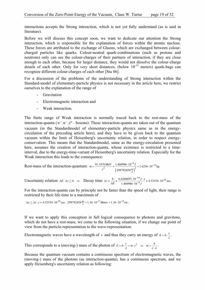
The finite range of Weak interaction is normally traced back to the rest-mass of the interaction-quanta ( 0, ,W W Z bosons): These interaction-quanta are taken out of the quantum vacuum (in the Standardmodel of elementary-particle physics same as in the energy-circulation of the preceding article here), and they have to be given back to the quantum vacuum within the limit of Heisenberg's uncertainty relation, in order to respect energy-conservation. This means that the Standardmodel, same as the energy-circulation presented here, assumes the creation of interaction-quanta, whose existence is restricted to a time-interval, due to the energy-time-variant of Heisenberg's uncertainty relation. Especially for the Weak interaction this leads to the consequence:
Rest-mass of the interaction-quantum:
825
2 2m
91.1876 1.460986 101.6256 10
299792458 s
MeV Jm kg
c
Uncertainty relation E t h Decay time 34
-268
6.6260693 104.53534 10 sec.
1.460986 10
h J st
E J
For the interaction-quanta can by principle not be faster than the speed of light, their range is restricted by their life-time to a maximum of
-26 -17 -15m4.53534 10 sec. 299792458 1.36 10 1.36 10sx t c Meter cm .
If we want to apply this conception in full logical consequence to photons and gravitons, which do not have a rest-mass, we come to the following situation, if we change our point of view from the particle-representation to the wave-representation:
Electromagnetic waves have a wavelength of and thus they carry an energy of cE h
.
This corresponds to a (moving-) mass of the photon of 2c hE h m c m
c
.
Because the quantum vacuum contains a continuous spectrum of electromagnetic waves, the (moving-) mass of the photons (as interaction-quanta), has a continuous spectrum, and we apply Heisenberg's uncertainty relation as following:

Conversion of the Zero-Point-Energy of the Vacuum, Claus W. Turtur page 20 of 52 xxx
2 2 1h c
E t h m c t h c t h t c tc
After a photon (as interaction-quantum of the electromagnetic interaction) is taken out of the quantum vacuum by an electric charge (which plays of the roll of a field source), the photon has to be given back to the quantum vacuum within the limit of Heisenberg's uncertainty relation, same as the interaction-quanta of Weak Interaction, which we discussed before. Because the photon propagates with the speed of light, it has to be given back to the quantum vacuum within the distance of propagation of s c t .
This has the consequence, that the range of the Electromagnetic interaction corresponds to the wavelength of the photon as the interaction-quantum, which are the wavelengths of the electromagnetic zero-point-waves of the quantum vacuum. Because the quantum vacuum contains a continuous spectrum of electromagnetic zero-point-waves, and the wavelengths go up to infinity, the range of the interaction has the same length, this is infinity. (Side-remark: A cutoff-radius of the wavelengths of the zero-point-waves for short wavelengths in the order of magnitude of the Planck-length is under discussion, in order to eliminate divergence-problems with the determination of the zero-point-energy of the quantum vacuum. A cutoff-radius for long wavelengths is not necessary and thus it was never under discussion [Whe 68].)
By the way: The concept presented for Electromagnetic interaction can be transferred to Gravitation identically. It is just necessary to replace the electromagnetic zero-point-waves by gravitational zero-point-waves and the photons by gravitons.
7. Solution of the discrepancy of the rest-mass of the field-sources During time (during centuries) the fields permanently spread out into the space (the universe). This is not the case for the Strong interaction and for the Weak interaction, because their range is finite, and after a short distance, they completely disappear, being fully re-absorbed by the vacuum. But Gravitation and Electromagnetic interaction propagates over infinite distance into the space. Thus their energy can be re-absorbed only partly but never completely by the vacuum. The consequence is, that the amount of field-energy (of the gravitational field, the magnetic field and the electric field) is permanently increasing during time. Due to energy-conservation, their counterpart, the vacuum-energy must decrease permanently during time. If we would know the amount and the distribution of electrical charges and ponderable masses in the universe, we could determine the amount of increasing field-energy and decreasing vacuum-energy as a function of time. This tells us that the information, that our universe consists of about two thirds of vacuum-energy is only a picture of the moment of observation - with regard to cosmological time-intervals. If we could observe the propagation of the fields for an infinite time-interval, we would come to the total field-energy, as known from literature. The prominent example for this calculation can be found in the widespread beginner’s-textbook by Richard Feynman, in which he demonstrates the determination energy and the mass of the electric field of the electron: From the electric field of the electron and its energy-density recording to our equations (1) and (2), Feynman determines the field-energy in the outside of the electron, using the classical electron’s radius of 152.818 10ER m (according to [COD 00]) as following:
2 220 02 2 4
0 0
1
2 2 4π 32π
Q Qu E
r r
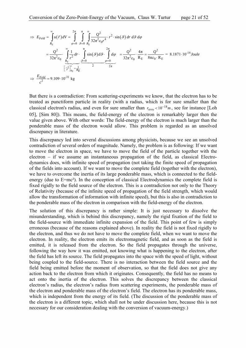
Conversion of the Zero-Point-Energy of the Vacuum, Claus W. Turtur page 21 of 52 xxx
2π π 22
2 400 0
π 2π2 2 2-14
2 2 2E 0 E0 00 0
2 2π1 1
sin32π
1 4πsin = 8.1871 10
R 8π R32π 32π
E E
E
RE
Feld
R R
R
r RE
QE u r dV r dr d d
r
Q Q Qdr d d Joule
r
-312
9.109 10 kgFeldE
c
But there is a contradiction: From scattering-experiments we know, that the electron has to be treated as punctiform particle in reality (with a radius, which is for sure smaller than the classical electron's radius, and even for sure smaller than 1810streur m , see for instance [Loh 05], [Sim 80]). This means, the field-energy of the electron is remarkably larger then the value given above. With other words: The field-energy of the electron is much larger than the ponderable mass of the electron would allow. This problem is regarded as an unsolved discrepancy in literature.
This discrepancy led into several discussions among physicists, because we see an unsolved contradiction of several orders of magnitude. Namely, the problem is as following: If we want to move the electron in space, we have to move the field of the particle together with the electron – if we assume an instantaneous propagation of the field, as classical Electro-dynamics does, with infinite speed of propagation (not taking the finite speed of propagation of the fields into account). If we want to move the complete field (together with the electron), we have to overcome the inertia of its large ponderable mass, which is connected to the field-energy (due to E=mc²). In the conception of classical Electrodynamics the complete field is fixed rigidly to the field source of the electron. This is a contradiction not only to the Theory of Relativity (because of the infinite speed of propagation of the field strength, which would allow the transformation of information with infinite speed), but this is also in contradiction to the ponderable mass of the electron in comparison with the field-energy of the electron.
The solution of this discrepancy is rather simple: It is just necessary to dissolve the misunderstanding, which is behind this discrepancy, namely the rigid fixation of the field to the field-source with immediate infinite expansion of the field. This point of few is simply erroneous (because of the reasons explained above). In reality the field is not fixed rigidly to the electron, and thus we do not have to move the complete field, when we want to move the electron. In reality, the electron emits its electromagnetic field, and as soon as the field is emitted, it is released from the electron. So the field propagates through the universe, following the way how it was emitted, not knowing what is happening to the electron, after the field has left its source. The field propagates into the space with the speed of light, without being coupled to the field-source. There is no interaction between the field source and the field being emitted before the moment of observation, so that the field does not give any action back to the electron from which it originates. Consequently, the field has no means to act onto the inertia of the electron. This solves the discrepancy between the classical electron’s radius, the electron’s radius from scattering experiments, the ponderable mass of the electron and ponderable mass of the electron’s field. The electron has its ponderable mass, which is independent from the energy of its field. (The discussion of the ponderable mass of the electron is a different topic, which shall not be under discussion here, because this is not necessary for our consideration dealing with the conversion of vacuum-energy.)
Conversion of the Zero-Point-Energy of the Vacuum, Claus W. Turtur page 22 of 52 xxx
This is one more example, from which we see, how the finite speed of propagation of the field (as a logical consequence of the Theory of Relativity) helps to solve old problems. After decades of years without any solution, the problem fell into oblivion – and here is the solution.
8. Microscopic vacuum-energy conversion This section has the purpose to demonstrate, that the conversion of vacuum-energy is not something exotic, which can only be achieved with hard effort and after overcoming many difficulties. In reality, the conversion of vacuum-energy is something very normal, which we observe every day in our normal life. In section 3 we saw, that every atom is a vacuum-energy-converter, and we know atoms from everyday’s life. We want to support this knowledge about the conversion of vacuum-energy by regarding the electrons in the atomic shell now, namely by demonstrating the connection between these shell-electrons and the vacuum-energy with a little calculation. Without the conversion of vacuum-energy, atoms could not exist by principle. From the theory of Stochastic Electrodynamics, we know that atoms convert vacuum-energy extremely efficient. We also know from section 2, that single electrons convert vacuum-energy very efficient. Without being supplied by vacuum-energy, electrons would decay within a tiny part of a second.
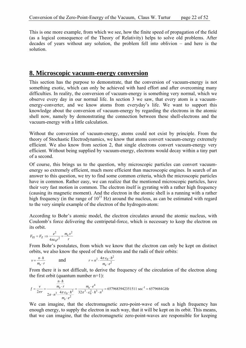
Of course, this brings us to the question, why microscopic particles can convert vacuum-energy so extremely efficient, much more efficient than macroscopic engines. In search of an answer to this question, we try to find some common criteria, which the microscopic particles have in common. Rather easy, we can realize that the mentioned microscopic particles, have their very fast motion in common. The electron itself is gyrating with a rather high frequency (causing its magnetic moment). And the electron in the atomic shell is a running with a rather high frequency (in the range of 1015 Hz) around the nucleus, as can be estimated with regard to the very simple example of the electron of the hydrogen-atom: According to Bohr’s atomic model, the electron circulates around the atomic nucleus, with Coulomb’s force delivering the centripetal-force, which is necessary to keep the electron on its orbit.
22
204
eEl Z
m veF F
rr
From Bohr’s postulates, from which we know that the electron can only be kept on distinct orbits, we also know the speed of the electrons and the radii of their orbits:
e
nv
m r
and
22 0
2
4
e
r nm e
From there it is not difficult, to derive the frequency of the circulation of the electron along the first orbit (quantum number n=1):
4-1
2 3 2 3 32 0 0
2
6579683942351511 sec 65796842 4 32
2
e e
e
n
m r m evf GHz
r nn
m e
We can imagine, that the electromagnetic zero-point-wave of such a high frequency has enough energy, to supply the electron in such way, that it will be kept on its orbit. This means, that we can imagine, that the electromagnetic zero-point-waves are responsible for keeping
Conversion of the Zero-Point-Energy of the Vacuum, Claus W. Turtur page 23 of 52 xxx
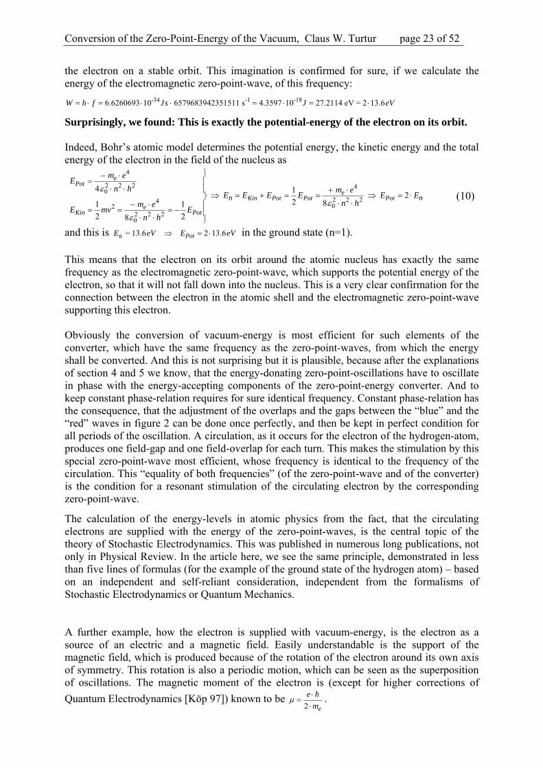
the electron on a stable orbit. This imagination is confirmed for sure, if we calculate the energy of the electromagnetic zero-point-wave, of this frequency:
-34 -1 -186.6260693 10 6579683942351511 s 4.3597 10 27.2114 eV = 2 13.6W h f Js J eV
Surprisingly, we found: This is exactly the potential-energy of the electron on its orbit. Indeed, Bohr’s atomic model determines the potential energy, the kinetic energy and the total energy of the electron in the field of the nucleus as
4
2 2 2 40
2 2 2402
2 2 20
4 12
2 81 1
2 28
ePot
eKin Pot Pot Pot
eKin Pot
n n
m eE
n h m eE E E E E E
n hm eE mv E
n h
(10)
and this is n = 13.6 2 13.6PotE eV E eV in the ground state (n=1). This means that the electron on its orbit around the atomic nucleus has exactly the same frequency as the electromagnetic zero-point-wave, which supports the potential energy of the electron, so that it will not fall down into the nucleus. This is a very clear confirmation for the connection between the electron in the atomic shell and the electromagnetic zero-point-wave supporting this electron. Obviously the conversion of vacuum-energy is most efficient for such elements of the converter, which have the same frequency as the zero-point-waves, from which the energy shall be converted. And this is not surprising but it is plausible, because after the explanations of section 4 and 5 we know, that the energy-donating zero-point-oscillations have to oscillate in phase with the energy-accepting components of the zero-point-energy converter. And to keep constant phase-relation requires for sure identical frequency. Constant phase-relation has the consequence, that the adjustment of the overlaps and the gaps between the “blue” and the “red” waves in figure 2 can be done once perfectly, and then be kept in perfect condition for all periods of the oscillation. A circulation, as it occurs for the electron of the hydrogen-atom, produces one field-gap and one field-overlap for each turn. This makes the stimulation by this special zero-point-wave most efficient, whose frequency is identical to the frequency of the circulation. This “equality of both frequencies” (of the zero-point-wave and of the converter) is the condition for a resonant stimulation of the circulating electron by the corresponding zero-point-wave.
The calculation of the energy-levels in atomic physics from the fact, that the circulating electrons are supplied with the energy of the zero-point-waves, is the central topic of the theory of Stochastic Electrodynamics. This was published in numerous long publications, not only in Physical Review. In the article here, we see the same principle, demonstrated in less than five lines of formulas (for the example of the ground state of the hydrogen atom) – based on an independent and self-reliant consideration, independent from the formalisms of Stochastic Electrodynamics or Quantum Mechanics. A further example, how the electron is supplied with vacuum-energy, is the electron as a source of an electric and a magnetic field. Easily understandable is the support of the magnetic field, which is produced because of the rotation of the electron around its own axis of symmetry. This rotation is also a periodic motion, which can be seen as the superposition of oscillations. The magnetic moment of the electron is (except for higher corrections of
Quantum Electrodynamics [Köp 97]) known to be 2 e
e
m
.
Conversion of the Zero-Point-Energy of the Vacuum, Claus W. Turtur page 24 of 52 xxx
Let us now look to this magnetic moment from the point of view of classical Electro-dynamics, from where we know it to be A I , with A cross section of the conductor-loop producing the magnetic moment and I electrical current responsible for the magnetic moment. If we bring both expressions for the magnetic moment together, we can calculate the electric current
22 e e
eI
A m r
.
Taking the classical electron’s radius as value for the radius of the conductor loop, and
calculating the electrical current as eI
T (with T= duration for one turn), we can calculate the
frequency of the spin of the electron. If we take additionally the fact into account, that the electric charge is regarded to be distributed homogeneously all over the surface of the electron (and not gyrating completely along the equator), we have to take and additional factor of 3
8
into account, and thus we come to the frequency -1315405884737 sec 15.4 GHz
8 e em r
.
This leads us to energy of -1
-34 -24 -515405884737 s6.6260693 10 1.62466 10 1.014 10 eV
2 W h f Js J
, of
the stimulating zero-point-wave. This is less than what we found for the orbital movement of the electron around the nucleus, but it is plausible, because the spin of the very small electron of course needs less energy than the gyration along an orbit, which is by many orders of magnitude larger than the electron itself. Nevertheless, the spin of the electron is supported by electromagnetic zero-point-waves, because there is no other source of energy, which can supply the electron in order to give him the possibility to maintain his magnetic field. The supply of the electron with zero-point-energy, which allows him to maintain his electrostatic field, is not yet understood, because it is not yet clear, where we find the motion and the oscillations, which are necessary to compress the wave trains of the zero-point-waves according to figure 2. There should be some zero-point oscillation of the electron itself, because the electron is also a particle described by Quantum-mechanics and by Stochastic Electrodynamics – and so it is not free from the zero-point oscillations of these theories. Here, some scientific work is still to be done. Nevertheless, it is sure that this supply is existing. This is clear on the one hand, because there is no other energy supply for the electron but the vacuum. And it is clear on the other hand from the verification experiment of [Tur 09]. In any case we see, that zero-point-energy converters improve their efficiency and power, as soon as the resonance frequency of the oscillating fields is increased. This is clear for magnetic zero-point-energy converters (which even can work as self-running engines) as well as for motionless converters. Central and most important aspect is always the frequency, with which the fields are moving, which are used for the conversion of the zero-point-energy. In order to optimize zero-point-energy converters, we should care about the following:
1. High-frequency of the field 2. Large number of particles, which take up the zero-point-energy 3. Maximization of the overlaps and the gaps between the “red” and the “blue” zero-
point wave trains, made by intervals with and without field being applied.

Conversion of the Zero-Point-Energy of the Vacuum, Claus W. Turtur page 25 of 52 xxx
9. Hydrogen-Converters
From literature, we know several Hydrogen-Converters. These are zero-point-energy converters, whose principle is based on the electrolysis of water-molecules, namely by dividing water-molecules into hydrogen and oxygen with a COP of much more than 100% (see for instance [Alm 09], [Bro 10]). This means, that the amount of electrical energy to be spent for the electrolysis is much less than the amount of chemical energy contained in the produced isolated gases of hydrogen and oxygen. This can be interpreted as following: For every Watt of electrical energy, which is necessary to keep the electrolysis running, the process gains many Watts of chemical energy, which can be transferred into thermal energy by burning the hydrogen with the oxygen (into water), or which can be transferred into electrical energy by giving the hydrogen and the oxygen to a fuel cell. By this means it is even possible to build a self running engine, producing permanently classical energy according to figure 3.
Fig. 3: Flux of energy in a self-running electrolyzer, driven by zero-point-energy.
The mechanism of this type of over-unity water-electrolysis is still under discussion [Nag 10]. Already clear is: The electrons in the atomic shell of the hydrogen- and the oxygen- atoms play the crucial role, because the term of “electrolysis” requires the separation of the covalent (chemical) bond of the atoms. (Please remind here the sections 3 and 8 of the present article.) It is a matter of course, that from there I get my hypothesis about the functioning principle of the over-unity water-electrolysis: If the electrons (which are supplied with zero-point-energy by nature in order to keep their orbits) can be oversupplied with zero-point-energy, it would be imaginable that they might be lifted into an excited state (an energy level above the ground state), from where they lose their covalent bonding, so that they will lose their capability to keep the hydrogen-atoms sticking to the oxygen-atoms. From section 8 we know, that high-frequency excitation gains zero-point-energy very efficiently, because the zero-point-waves of high frequencies carry a large amount of energy according to W h f . So probably it would be sensible to drive of the over-unity water-electrolysis with a rather high-frequency. But we do not expect, that the frequency will just simply increase the efficiency, because of the frequency of the excitation by zero-point-waves should be in the resonance with the frequency, which the bonding-electrons of the water-molecules needs to be lifted into an excited state. Maybe a good choice for a trial of the excitation-frequency could be the frequency, which is necessary to support the 2s-state of the hydrogen-atom, in order to lift the electron from the 1s-state to the 2s-state. This would be
4-18
2 2 2 20
-18
-34
2 13.62 6.8 1.0895 10
4 2
1.0895 101644232788811913Hz 1644.23THz
6.62607 10
ePot
Pot
nm e eV
E E eV Jn h
E Jf
h J s

Conversion of the Zero-Point-Energy of the Vacuum, Claus W. Turtur page 26 of 52 xxx
This is not a low frequency, but perhaps it can be produced as a component of the Fourier-spectrum of extremely short pulses to the electrodes. Perhaps an alternative for its production
might be an optical method (to produce UV-light of 182c
nmf
), but it is not clear, how an
optical frequency can be brought to an electrode. Probably it is also sensible, to try not only this one frequency, but to try the complete frequency-range in the order of magnitude under discussion, because the covalent bonding of the hydrogen-atom to the oxygen-atom influences the energy-levels of the electrons.
10. An uncomplicated setup
This is the very first time that an algorithm for the construction of zero-point-energy converters is presented. Thus, the computer-program was developed as uncomplicated as possible, in order to make it understandable to everybody. For the conversion of zero-point-energy is not something exotic, it is not difficult to find a very simple setup (as a basis for the analysis in our DFEM-algorithm), which can fulfill this task: For the sake of simplicity, we take a one-dimensional example, and it is already sufficient to connect two masses with a helical spring, in order to build up a simple oscillator – nothing more – this is all we need. The only addition we will need is some electrical charge on the bodies No.1 and 2, or some magnets. The arrangement is drawn in figure 4 as it could be seen in every beginner’s textbook.
Fig. 4: Two masses, which are connected by a helical spring, can perform an oscillation.
If we want to trace back the example of figure 4 directly to a simple beginner’s example, we can fix one ponderable mass with the use of a helical spring directly to a wall (as drawn in blue) in the middle of the setup and observe harmonic oscillations according to the differ-ential-equation (11) without friction and without excitation. The solution according to equation (12) is generally known as:
Differential-equation 1 1 0m x D x (resp. 2 2 0m x D x ) (11)Solution 0cosx t A t ,
with the symbols as usual in literature. (12)
Of course, the amplitude is constant, and there is no conversion of zero-point-energy in this example.
But if we put some electrical charge on the bodies 1m and 2m , or if we replace them by two magnets, an additional force will occur (it can be attractive or repulsive), which depends on the distance between the charged spheres or magnets. For the further course of our article, let us chose the direction of this interacting force to be attractive. In the case of electrically charged spheres, the force follows the (first) coulomb's law according to (13); in the case of permanent magnets the force follows the (second) coulomb's
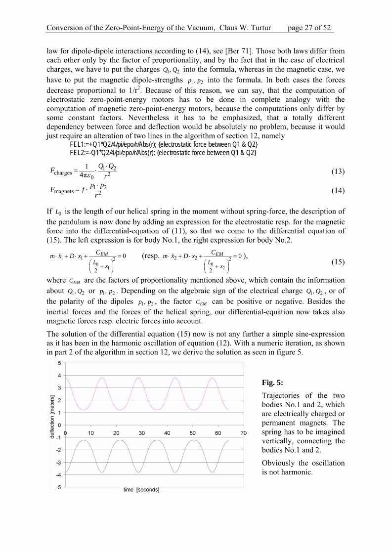
Conversion of the Zero-Point-Energy of the Vacuum, Claus W. Turtur page 27 of 52 xxx
law for dipole-dipole interactions according to (14), see [Ber 71]. Those both laws differ from each other only by the factor of proportionality, and by the fact that in the case of electrical charges, we have to put the charges 1 2,Q Q into the formula, whereas in the magnetic case, we have to put the magnetic dipole-strengths 1 2,p p into the formula. In both cases the forces decrease proportional to 1/r2. Because of this reason, we can say, that the computation of electrostatic zero-point-energy motors has to be done in complete analogy with the computation of magnetic zero-point-energy motors, because the computations only differ by some constant factors. Nevertheless it has to be emphasized, that a totally different dependency between force and deflection would be absolutely no problem, because it would just require an alteration of two lines in the algorithm of section 12, namely FEL1:=+Q1*Q2/4/pi/epo/r/Abs(r); {electrostatic force between Q1 & Q2} FEL2:=-Q1*Q2/4/pi/epo/r/Abs(r); {electrostatic force between Q1 & Q2}
1 2charges 2
0
14π
Q QF
r (13)
1 2magnets 2
fp p
Fr
(14)
If 0L is the length of our helical spring in the moment without spring-force, the description of the pendulum is now done by adding an expression for the electrostatic resp. for the magnetic force into the differential-equation of (11), so that we come to the differential equation of (15). The left expression is for body No.1, the right expression for body No.2.
01
1 1 2
2
0EM
Lx
Cm x D x
(resp. 0
2
2 2 2
2
0EM
Lx
Cm x D x
), (15)
where EMC are the factors of proportionality mentioned above, which contain the information about 1 2,Q Q or 1 2,p p . Depending on the algebraic sign of the electrical charge 1 2,Q Q , or of the polarity of the dipoles 1 2,p p , the factor EMC can be positive or negative. Besides the inertial forces and the forces of the helical spring, our differential-equation now takes also magnetic forces resp. electric forces into account.
The solution of the differential equation (15) now is not any further a simple sine-expression as it has been in the harmonic oscillation of equation (12). With a numeric iteration, as shown in part 2 of the algorithm in section 12, we derive the solution as seen in figure 5.
Fig. 5:
Trajectories of the two bodies No.1 and 2, which are electrically charged or permanent magnets. The spring has to be imagined vertically, connecting the bodies No.1 and 2.
Obviously the oscillation is not harmonic.

Conversion of the Zero-Point-Energy of the Vacuum, Claus W. Turtur page 28 of 52 xxx
Obviously classical potential energy (of the electrical or the magnetic field) is converted into the energy of spring energy and kinetic energy. Thus, we have an energy-conversion between these three types of classical energy. Of course zero-point-energy is still not under discussion. The amplitudes are constant, confirming the conservation of classical energy. The computer-simulation of the motion can be found in part 2 in the source-code printed in section 12. Because up to here, we did not yet deal with the zero-point-energy conversion, the algorithm is still a classical static FEM-algorithm (with only two elements).
11. Introducing Dynamics: From FEM to DFEM We now want to insert the finite speed of propagation of the electric field resp. the magnetic field into the considerations of figure 4 and section 10. In the static theory of electricity, the duration for the propagation of these fields is neglected. This means, that the speed of propa-gation of the fields is approximated to be infinitely fast. Of course, this is in clear contra-diction to the Theory of Relativity, according to which the speed of light is a principle upper limit to all velocity and speed at all. So we regard the static theory of electricity as an approximation, which works rather well in many classical cases for engineering purpose, but which is not sufficient for the explanation of the zero-point-energy motors by principle (see above). Thus we decide to reject this approximation now, in order to make the conversion of zero-point-energy understandable.
By the way, the speed of propagation of the fields is the speed of light only inside the vacuum. Inside matter, the fields propagate less fast.
Consequently, we have to replace equation (15) and figure 5, which are based on the approximation of infinite speed of propagation of the fields, by a more precise consideration. This is what we do now: For the solution of equation (15), the forces in part 2 of the algorithm (see section 12) had been calculated only with the use of the static version of coulomb’s law. For the dynamic computation, we now have to accept the fields of interaction as self-reliant physical entities, and we have to take their finite speed of propagation into account, as illustrated in figure 6. There we see two bodies moving to the left and to the right, and the time-dependant development of the situation is plotted in three steps from the top to the bottom.
At the moment at the interacting partner No.1 (magnet or charge) is at the position 1,ax and
the interacting partner No.2 is at the position 2,ax . At the moment at , No.1 emits a field,
which propagates among others also into the direction towards No.2 (red arrow). This part of the field is responsible for force of No.1 acting on No.2. This field(-package) now approaches towards No. 2, but at the same time, No.1 also moves a little bit to the right side, this means, that No.1 follows the direction of the field. But No.2 moves from the right to the left side, this is the direction towards the field(-package). We can see this development, when we follow the course of the time from at to bt . But finally we further follow the course of the time until we reach ct . This is the moment, at which the field reaches the partner No.2.
For the computation of coulomb's law we now face the question: Which field-strength does partner No.2 feel in this moment ?
The answer is clear: We use Coulomb's law according to equation (13) or (14), and we apply the distance which the field had to pass really. This is the distance marked with the blue arrow in figure 6. This means that No.2 feels less field strength in the moment ct , then it
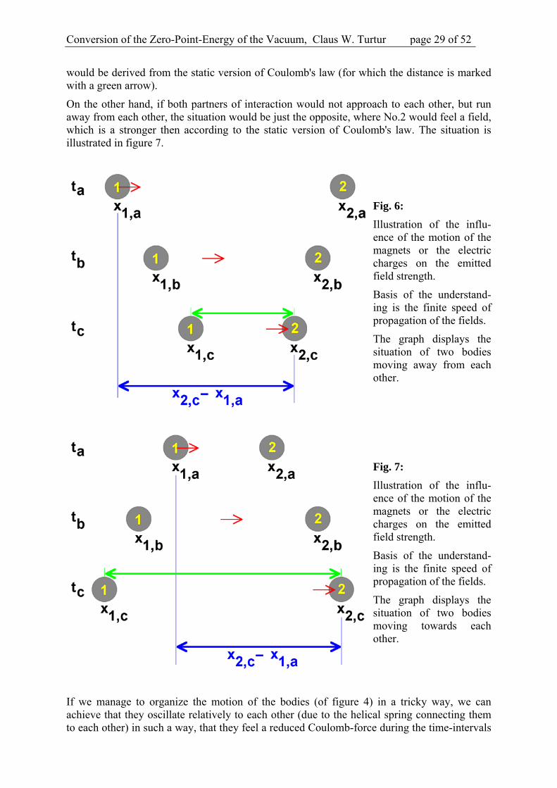
Conversion of the Zero-Point-Energy of the Vacuum, Claus W. Turtur page 29 of 52 xxx
would be derived from the static version of Coulomb's law (for which the distance is marked with a green arrow).
On the other hand, if both partners of interaction would not approach to each other, but run away from each other, the situation would be just the opposite, where No.2 would feel a field, which is a stronger then according to the static version of Coulomb's law. The situation is illustrated in figure 7.
Fig. 6:
Illustration of the influ-ence of the motion of the magnets or the electric charges on the emitted field strength.
Basis of the understand-ing is the finite speed of propagation of the fields.
The graph displays the situation of two bodies moving away from each other.
Fig. 7:
Illustration of the influ-ence of the motion of the magnets or the electric charges on the emitted field strength.
Basis of the understand-ing is the finite speed of propagation of the fields.
The graph displays the situation of two bodies moving towards each other.
If we manage to organize the motion of the bodies (of figure 4) in a tricky way, we can achieve that they oscillate relatively to each other (due to the helical spring connecting them to each other) in such a way, that they feel a reduced Coulomb-force during the time-intervals
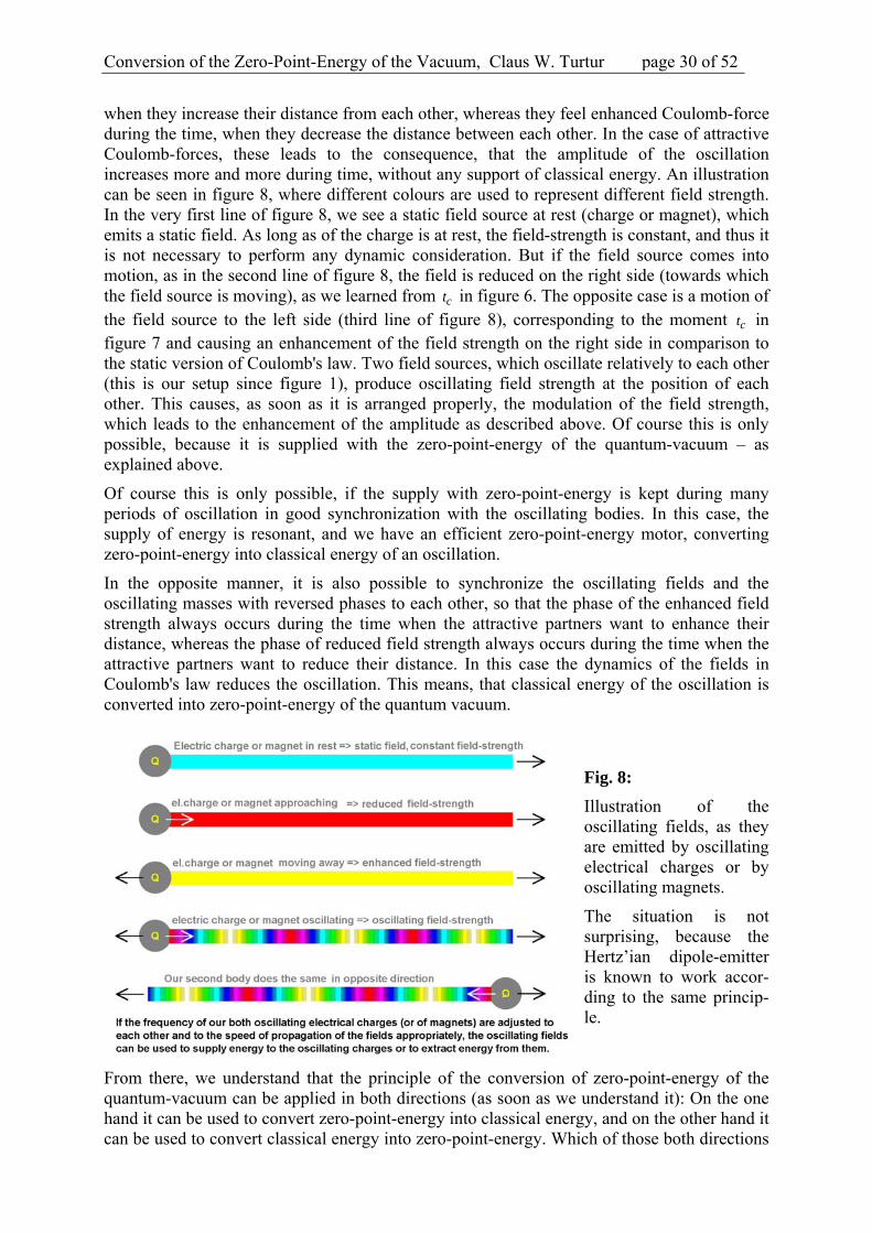
Conversion of the Zero-Point-Energy of the Vacuum, Claus W. Turtur page 30 of 52 xxx
when they increase their distance from each other, whereas they feel enhanced Coulomb-force during the time, when they decrease the distance between each other. In the case of attractive Coulomb-forces, these leads to the consequence, that the amplitude of the oscillation increases more and more during time, without any support of classical energy. An illustration can be seen in figure 8, where different colours are used to represent different field strength. In the very first line of figure 8, we see a static field source at rest (charge or magnet), which emits a static field. As long as of the charge is at rest, the field-strength is constant, and thus it is not necessary to perform any dynamic consideration. But if the field source comes into motion, as in the second line of figure 8, the field is reduced on the right side (towards which the field source is moving), as we learned from ct in figure 6. The opposite case is a motion of the field source to the left side (third line of figure 8), corresponding to the moment ct in figure 7 and causing an enhancement of the field strength on the right side in comparison to the static version of Coulomb's law. Two field sources, which oscillate relatively to each other (this is our setup since figure 1), produce oscillating field strength at the position of each other. This causes, as soon as it is arranged properly, the modulation of the field strength, which leads to the enhancement of the amplitude as described above. Of course this is only possible, because it is supplied with the zero-point-energy of the quantum-vacuum – as explained above.
Of course this is only possible, if the supply with zero-point-energy is kept during many periods of oscillation in good synchronization with the oscillating bodies. In this case, the supply of energy is resonant, and we have an efficient zero-point-energy motor, converting zero-point-energy into classical energy of an oscillation.
In the opposite manner, it is also possible to synchronize the oscillating fields and the oscillating masses with reversed phases to each other, so that the phase of the enhanced field strength always occurs during the time when the attractive partners want to enhance their distance, whereas the phase of reduced field strength always occurs during the time when the attractive partners want to reduce their distance. In this case the dynamics of the fields in Coulomb's law reduces the oscillation. This means, that classical energy of the oscillation is converted into zero-point-energy of the quantum vacuum.
Fig. 8:
Illustration of the oscillating fields, as they are emitted by oscillating electrical charges or by oscillating magnets.
The situation is not surprising, because the Hertz’ian dipole-emitter is known to work accor-ding to the same princip-le.
From there, we understand that the principle of the conversion of zero-point-energy of the quantum-vacuum can be applied in both directions (as soon as we understand it): On the one hand it can be used to convert zero-point-energy into classical energy, and on the other hand it can be used to convert classical energy into zero-point-energy. Which of those both directions

Conversion of the Zero-Point-Energy of the Vacuum, Claus W. Turtur page 31 of 52 xxx
is realized in an engine is mainly a question of the adjustment of the system-parameters. Especially the following both system-parameters have to be adjusted appropriately to each other: - the speed of propagation of the fields and - the speed of motion of the moving field sources.
In our example-algorithm this means, that we have to adjust the deflections and the amplitude of the oscillating bodies, their ponderable masses, Hooke’s spring force constant, and finally of course the electrical charges, which supply the Coulomb-forces necessary to convert zero-point-energy appropriately to each other. Instead of electrical charges, it would also be possib-le to use permanent magnets and to include the adjustment of their dipole-strengths into the adjustment of the system-parameters.
In order to prove all these statements, within the preceding work, a dynamic Finite-element algorithm (DFEM) was developped, which is a very short and easy to understand. It realizes the oscillation of two electrically charged spheres with a spring as drawn in figure 4, taking the finite speed of propagation of the Coulomb-field into account when analyzing the oscillation. This means that we have the same geometrical setup as we had for our static consideration leading to figure 5. But due to the fact, that we now perform a dynamic analysis, we derive the deflections of figure 9, figures 10 and figure 11. Therefore, the adjustment of the system-parameters (in our algorithm) is given as following:
With Fig.9: - speed of propagation of the fields 1.4mc s - electrical charges 1Q and 2Q = 53 10 C per each - Hooke’s spring force constant 2.7 ND m - length of the unloaded helical spring 8.0RLL m - starting-position of the bodies’ motion at 1 3.0x m and 2 3.0x m .
As can be seen, the amplitude increases rather fast at the begin of the oscillation. Obviously the motion of the bodies and the motion of the Coulomb-fields are adjusted in such a way to each other, that the oscillation gains energy from the quantum vacuum rather efficiently. But we further observe, that there is a certain limit for the amplitudes. This comes from the fact, that the speed of the motion of the bodies reaches a value in comparison with the speed of the propagation of the fields, that it will not be possible to gain more energy from the quantum vacuum than seen in this oscillation after time “30 seconds”. This means that the gain of energy from the quantum vacuum is saturated at these system-parameters reached here, and the amplitude will become constant. But it must be said: If we would extract mechanical energy from this oscillation (with constant amplitude), the mechanical extraction of energy would act back on the amplitude (as seen in section 14), but in this moment the re-gain of energy from the quantum vacuum would be enhanced, so that the amplitude would still be kept at its constant value (as long as we do not extract too much mechanical energy). The amount of mechanical energy which we can extract, is the engine-power, which we can gain from the zero-point-energy of the quantum vacuum in this mode of the operation of the zero-point-energy motor.
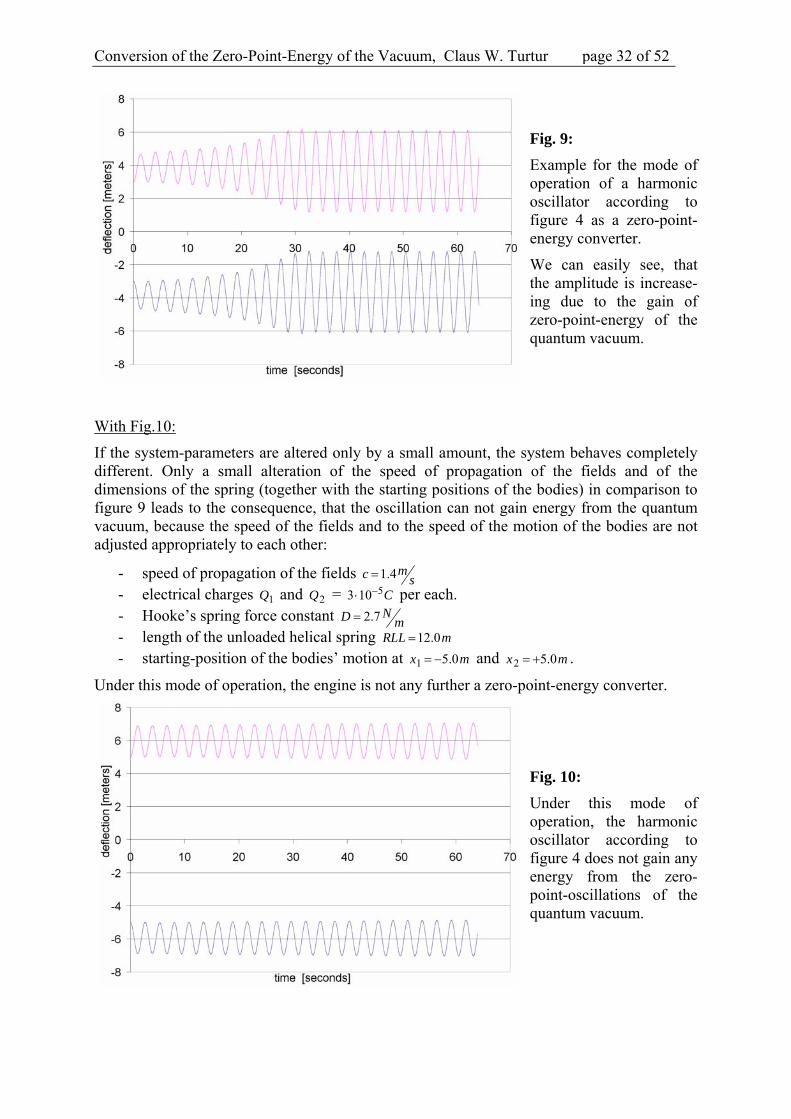
Conversion of the Zero-Point-Energy of the Vacuum, Claus W. Turtur page 32 of 52 xxx
Fig. 9:
Example for the mode of operation of a harmonic oscillator according to figure 4 as a zero-point-energy converter.
We can easily see, that the amplitude is increase-ing due to the gain of zero-point-energy of the quantum vacuum.
With Fig.10:
If the system-parameters are altered only by a small amount, the system behaves completely different. Only a small alteration of the speed of propagation of the fields and of the dimensions of the spring (together with the starting positions of the bodies) in comparison to figure 9 leads to the consequence, that the oscillation can not gain energy from the quantum vacuum, because the speed of the fields and to the speed of the motion of the bodies are not adjusted appropriately to each other:
- speed of propagation of the fields 1.4mc s - electrical charges 1Q and 2Q = 53 10 C per each. - Hooke’s spring force constant 2.7 ND m - length of the unloaded helical spring 12.0RLL m - starting-position of the bodies’ motion at 1 5.0x m and 2 5.0x m .
Under this mode of operation, the engine is not any further a zero-point-energy converter.
Fig. 10:
Under this mode of operation, the harmonic oscillator according to figure 4 does not gain any energy from the zero-point-oscillations of the quantum vacuum.
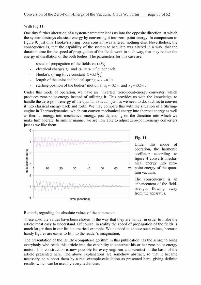
Conversion of the Zero-Point-Energy of the Vacuum, Claus W. Turtur page 33 of 52 xxx
With Fig.11:
One tiny further alteration of a system-parameter leads us into the opposite direction, at which the system destroys classical energy by converting it into zero-point-energy. In comparison to figure 9, just only Hooke’s spring force constant was altered, nothing else. Nevertheless, the consequence is, that the capability of the system to oscillate was altered in a way, that the duration time for the speed of propagation of the fields work in such way, that they reduce the energy of oscillation of the both bodies. The parameters for this case are:
- speed of propagation of the fields 1.4mc s - electrical charges 1Q and 2Q = 53 10 C per each - Hooke’s spring force constant 3.5ND m - length of the unloaded helical spring 8.0RLL m - starting-position of the bodies’ motion at 1 3.0x m and 2 3.0x m .
Under this mode of operation, we have an “inverted” zero-point-energy converter, which produces zero-point-energy instead of utilizing it. This provides us with the knowledge, to handle the zero-point-energy of the quantum vacuum just as we need to do, such as to convert it into classical energy back and forth. We may compare this with the situation of a Stirling-engine in Thermodynamics, which can convert mechanical energy into thermal energy as well as thermal energy into mechanical energy, just depending on the direction into which we make him operate. In similar manner we are now able to adjust zero-point-energy converters just as we like them.
Fig. 11:
Under this mode of operation, the harmonic oscillator according to figure 4 converts mecha-nical energy into zero-point-energy of the quan-tum vacuum.
The consequence is an enhancement of the field-strength flowing away from the apparatus.
Remark, regarding the absolute values of the parameters:
These absolute values have been chosen in the way that they are handy, in order to make the article most easy to understand. Of course, in reality the speed of propagation of the fields is much larger than in our little numerical example. We decided to choose such values, because handy figures are easier to fit into the reader’s imagination.
The presentation of the DFEM-computer-algorithm in this publication has the sense, to bring everybody who reads this article into the capability to construct his or her zero-point-energy motor. This construction is now possible for every engineer and scientist on the basis of the article presented here. The above explanations are somehow abstract, so that it became necessary, to support them by a real example-calculation as presented here, giving definite results, which can be used by every technician.
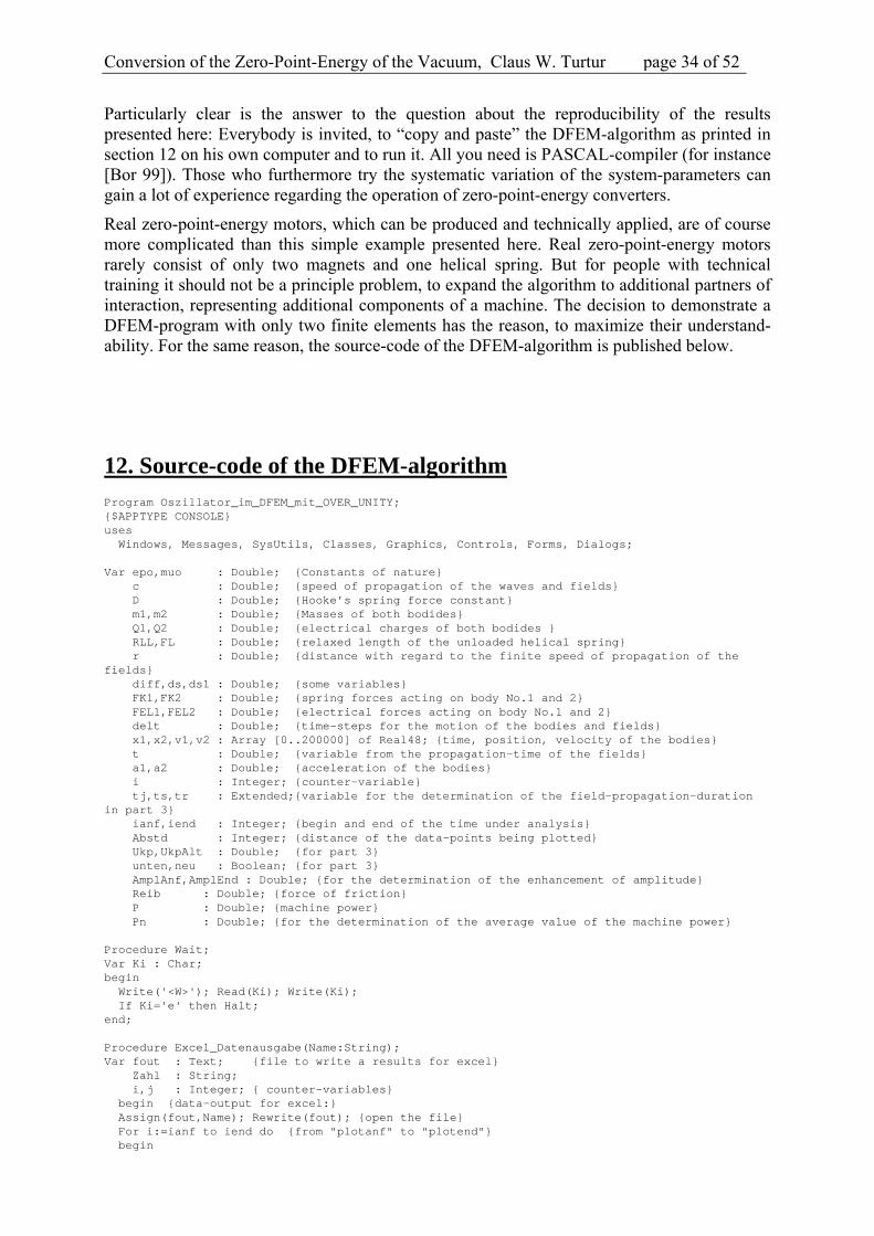
Conversion of the Zero-Point-Energy of the Vacuum, Claus W. Turtur page 34 of 52 xxx
Particularly clear is the answer to the question about the reproducibility of the results presented here: Everybody is invited, to “copy and paste” the DFEM-algorithm as printed in section 12 on his own computer and to run it. All you need is PASCAL-compiler (for instance [Bor 99]). Those who furthermore try the systematic variation of the system-parameters can gain a lot of experience regarding the operation of zero-point-energy converters.
Real zero-point-energy motors, which can be produced and technically applied, are of course more complicated than this simple example presented here. Real zero-point-energy motors rarely consist of only two magnets and one helical spring. But for people with technical training it should not be a principle problem, to expand the algorithm to additional partners of interaction, representing additional components of a machine. The decision to demonstrate a DFEM-program with only two finite elements has the reason, to maximize their understand-ability. For the same reason, the source-code of the DFEM-algorithm is published below.
12. Source-code of the DFEM-algorithm
Program Oszillator_im_DFEM_mit_OVER_UNITY; {$APPTYPE CONSOLE} uses Windows, Messages, SysUtils, Classes, Graphics, Controls, Forms, Dialogs; Var epo,muo : Double; {Constants of nature} c : Double; {speed of propagation of the waves and fields} D : Double; {Hooke’s spring force constant} m1,m2 : Double; {Masses of both bodides} Q1,Q2 : Double; {electrical charges of both bodides } RLL,FL : Double; {relaxed length of the unloaded helical spring} r : Double; {distance with regard to the finite speed of propagation of the fields} diff,ds,ds1 : Double; {some variables} FK1,FK2 : Double; {spring forces acting on body No.1 and 2} FEL1,FEL2 : Double; {electrical forces acting on body No.1 and 2} delt : Double; {time-steps for the motion of the bodies and fields} x1,x2,v1,v2 : Array [0..200000] of Real48; {time, position, velocity of the bodies} t : Double; {variable from the propagation-time of the fields} a1,a2 : Double; {acceleration of the bodies} i : Integer; {counter-variable} tj,ts,tr : Extended;{variable for the determination of the field-propagation-duration in part 3} ianf,iend : Integer; {begin and end of the time under analysis} Abstd : Integer; {distance of the data-points being plotted} Ukp,UkpAlt : Double; {for part 3} unten,neu : Boolean; {for part 3} AmplAnf,AmplEnd : Double; {for the determination of the enhancement of amplitude} Reib : Double; {force of friction} P : Double; {machine power} Pn : Double; {for the determination of the average value of the machine power} Procedure Wait; Var Ki : Char; begin Write('<W>'); Read(Ki); Write(Ki); If Ki='e' then Halt; end; Procedure Excel_Datenausgabe(Name:String); Var fout : Text; {file to write a results for excel} Zahl : String; i,j : Integer; { counter-variables} begin {data-output for excel:} Assign(fout,Name); Rewrite(fout); {open the file} For i:=ianf to iend do {from "plotanf" to "plotend"} begin

Conversion of the Zero-Point-Energy of the Vacuum, Claus W. Turtur page 35 of 52 xxx
If (i mod Abstd)=0 then begin { the first argument is the time:} Str(i*delT:10:5,Zahl); For j:=1 to Length(Zahl) do begin {replace decimal-points by commata} If Zahl[j]<>'.' then write(fout,Zahl[j]); If Zahl[j]='.' then write(fout,','); end; Write(fout,chr(9)); {Tabulator for data-separation} { The first function is the Position of particle No. 1:} Str(x1[i]:10:5,Zahl); For j:=1 to Length(Zahl) do begin { replace decimal-points by commata } If Zahl[j]<>'.' then write(fout,Zahl[j]); If Zahl[j]='.' then write(fout,','); end; Write(fout,chr(9)); {Tabulator for data-separation } { second column: Position of body 2:} Str(x2[i]:10:5,Zahl); For j:=1 to Length(Zahl) do begin { replace decimal-points by commata } If Zahl[j]<>'.' then write(fout,Zahl[j]); If Zahl[j]='.' then write(fout,','); end; Write(fout,chr(9)); {Tabulator for data-separation } { third column: velocity of body 1:} Str(v1[i]:10:5,Zahl); For j:=1 to Length(Zahl) do begin { replace decimal-points by commata } If Zahl[j]<>'.' then write(fout,Zahl[j]); If Zahl[j]='.' then write(fout,','); end; Write(fout,chr(9)); {Tabulator for data-separation } { fourth column: velocity of body 2:} Str(v2[i]:10:5,Zahl); For j:=1 to Length(Zahl) do begin { replace decimal-points by commata } If Zahl[j]<>'.' then write(fout,Zahl[j]); If Zahl[j]='.' then write(fout,','); end; Writeln(fout,''); {line-feed for data-separation} end; end; Close(fout); end; Begin {Main program} { Initialisation: } D:=0; r:=0; {Avoid Delphi-Messages} epo:=8.854187817E-12;{As/Vm} {Magnetic field-constant } muo:=4*pi*1E-7;{Vs/Am} {elektric field-constant } c:=Sqrt(1/muo/epo);{m/s} {speed of light } m1:=1;{kg} {mass of body 1} m2:=1;{kg} {mass of body 2} delt:=1E-3;{sec.} {Equidistant time-steps for the calculation of the motion} ianf:=0; iend:=100000; {number of the first and the last time.-step } Abstd:=2; {to plot every Abstd-th data-point} Writeln('Oscillator in DFEM with OVER-UNITY:'); Writeln('epo=',epo:20,'; muo=',muo:20,'; c=',c:20); Writeln('m1,m2=',m1:15,', ',m2:15,'; D=',D:15); Writeln; { Begin of the Main Program} { Part 1 had been preparations for the program-development, not interesting any further} { Teil 2: Test -> anharmonic oscillation, with electrical charge or magnet: STATIC !} For i:=ianf to iend do begin x1[i]:=0; x2[i]:=0; {assign the positions to zero} v1[i]:=0; v2[i]:=0; {assign the velocities to zero} end; i:=0; {t:=i*delT;} {time in steps of delt.} Q1:=2.01E-5{C}; Q2:=2.01E-5{C}; {electrical charge of both bodies}

Conversion of the Zero-Point-Energy of the Vacuum, Claus W. Turtur page 36 of 52 xxx
D:=0.20;{N/m} {Hooke’s spring force constant } RLL:=6.0;{m} {length of the spring without force} {rest-position of the bodies: +/-RLL/2} x1[0]:=-3.8; x2[0]:=+3.8; {starting-positions of the bodies} v1[0]:=00.00; v2[0]:=00.00; { starting-velocities of the bodies } {Now we begin the determination of the motion, step-by-step:} Repeat i:=i+1; FL:=x2[i-1]-x1[i-1]; {length of the spring} FK1:=(FL-RLL)*D; {spring-force, positive pulls to the right side, negative to the left} FK2:=(RLL-FL)*D; {spring-force, positive pulls to the right side, negative to the left} FEL1:=0; FEL2:=0; If FL<=1E-20 then begin Writeln; Writeln('Exception: Spring too much compressed in Part 2 at step ',i); Excel_Datenausgabe('XLS-Nr-02.DAT'); Writeln('Data have been stored at "XLS-Nr-02.DAT", then termination of algorithm.'); Wait; Halt; end; If FL>1E-20 then begin FEL1:=+Q1*Q2/4/pi/epo/FL/Abs(FL); {electrostatic force between Q1 & Q2} FEL2:=-Q1*Q2/4/pi/epo/FL/Abs(FL); {electrostatic force between Q1 & Q2} end; {Check:} If i=1 then Writeln('El.-force: ',FEL1,' and ',FEL2,' Newton'); {Check:} If i=1 then Writeln('Spring-force: ',FK1, ' and ',FK2,' Newton'); a1:=(FK1+FEL1)/m1; a2:=(FK2+FEL2)/m2; {acceleration of the bodies} v1[i]:=v1[i-1]+a1*delt; {alteration of the speed of body 1} v2[i]:=v2[i-1]+a2*delt; {alteration of the speed of body 2} x1[i]:=x1[i-1]+v1[i-1]*delt; {alteration of the position of body 1} x2[i]:=x2[i-1]+v2[i-1]*delt; {alteration of the position of body 2} Until i=iend; Excel_Datenausgabe('XLS-Nr-02.DAT'); {position and speed as a function of time} Writeln('Part 2 is ready.'); { Part 3: Test -> Propagation of the fields with finite speed} P:=0; Pn:=0; {assign the machine-power to zero} For i:=ianf to iend do begin x1[i]:=0; x2[i]:=0; {assign the positions to zero} v1[i]:=0; v2[i]:=0; {assign the velocities to zero} end; i:=0; {counter for the position and velocity} c:=1.4; {Sqrt(1/muo/epo);{m/s} {assign the speed of propagation of the fields here} Q1:=3E-5{C}; Q2:=3E-5{C}; {electrical charge of the bodies} D:=2.7;{N/m} { Hooke’s spring force constant } RLL:=8.0;{m} {length of the spring without force} {rest-position of the bodies: +/-RLL/2} x1[0]:=-3.0; x2[0]:=+3.0; {starting-position of the bodies} v1[0]:=00.00; v2[0]:=00.00; {starting-velocity of the bodies } Ukp:=x2[0]; UkpAlt:=Ukp; unten:=true; neu:=true; {first reversal point} Writeln('reversal-point: ',Ukp:12:6,' m '); {Now we begin the determination of the motion, step-by-step:} Repeat i:=i+1; FL:=x2[i-1]-x1[i-1]; {length of the spring} FK1:=(FL-RLL)*D; {spring-force, positive pulls to the right side, negative to the left} FK2:=(RLL-FL)*D; {spring-force, positive pulls to the right side, negative to the left} { determination of the Field-motion-duration, Field-motion-distance, and Field-strength} FEL1:=0; FEL2:=0; tj:=i; ts:=i; {i mesures the time} {Start the iteration with natural figures:} { Writeln('tj=',tj*delt:9:5,' ts=',ts*delt:9:5,'=>',x2[Round(tj)]-x1[Round(ts)]-c*(tj-ts)*delt:9:5); } Repeat ts:=ts-1; diff:=x2[Round(tj)]-x1[Round(ts)]-c*(tj-ts)*delt; { Writeln('tj=',tj*delt:9:5,' ts=',ts*delt:9:5,'=>',diff:9:5); } Until ((diff<0)or(ts<=0)); If diff>=0 then {before the motion begin at t=0, the bodies have been in rest.} begin r:=x2[Round(tj)]-x1[0]; { Writeln('diff>=0; r=',r); } end; If diff<0 then {linear interpolation to determine the fraction after the comma} begin
Conversion of the Zero-Point-Energy of the Vacuum, Claus W. Turtur page 37 of 52 xxx
{ Writeln('diff<0 ==> tj=',tj,' ts=',ts); Write('x2[',Round(tj),']=',x2[Round(tj)]:13:9); Write(' und x1[',Round(ts),']=',x1[Round(ts)]:13:9); Write(' und x1[',Round(ts+1),']=',x1[Round(ts+1)]:13:9); Writeln; } ds:=x2[Round(tj)]-x1[Round(ts)]-c*(tj-ts)*delt; ds1:=x2[Round(tj)]-x1[Round(ts+1)]-c*(tj-(ts+1))*delt; { Writeln('ds1=',ds1:13:9,' und ds=',ds:13:9); } tr:=ts*delt+delt*(-ds)/(ds1-ds); {for linear interpolation} tj:=tj*delt; { Write('tj=',tj:13:9,' und tr_vor=',tr:13:9); } tr:=(tj-tr); {interpolated moment of field-emission} r:=c*tr; {interpolated real distance} { Writeln(' und tr=',tr:13:9,' und r=',r:13:9); } end; If r<=1E-10 then begin Writeln; Writeln('Exception: Spring too much compressed in Part 3 at step ',i); Excel_Datenausgabe('XV-03.DAT'); Writeln('Data have been stored at "XV-03.DAT", then termination of algorithm.'); Wait; Halt; end; If r>1E-10 then {Now insert data into Coulomb’s law:} begin FEL1:=+Q1*Q2/4/pi/epo/r/Abs(r); {electrostatic force between Q1 & Q2} FEL2:=-Q1*Q2/4/pi/epo/r/Abs(r); { electrostatic force between Q1 & Q2} end; Reib:=0.2; {friction: computation begins here.} If i>=10000 then begin If FEL1>0 then FEL1:=FEL1-Reib; If FEL1<0 then FEL1:=FEL1+Reib; If FEL2>0 then FEL2:=FEL2-Reib; If FEL2<0 then FEL2:=FEL2+Reib; P:=P+Reib*Abs(x1[i]-x1[i-1])/delt; Pn:=Pn+1; end; {Friction: computation ends here.} {Check:} If i=1 then Writeln('El.-force: ',FEL1,' and ',FEL2,' Newton'); {Check:} If i=1 then Writeln('spring-force: ',FK1, ' and ',FK2,' Newton'); a1:=(FK1+FEL1)/m1; a2:=(FK2+FEL2)/m2; {acceleration of the bodies} v1[i]:=v1[i-1]+a1*delt; {alteration of the speed of body 1} v2[i]:=v2[i-1]+a2*delt; {alteration of the speed of body 2} x1[i]:=x1[i-1]+v1[i-1]*delt; {alteration of the position of body 1} x2[i]:=x2[i-1]+v2[i-1]*delt; {alteration of the position of body 2} { If (i mod 1000)=0 then Writeln ('Feldstaerke= ',Q1/4/pi/epo/r/Abs(r),' N/C'); } { determination of the reversal-points, for determination of the amplitude’s-enhancement:} If unten then begin If x2[i]>Ukp then begin Ukp:=x2[i]; end; If x2[i]<Ukp then begin Writeln('reversal-point: ',Ukp:12:6,' m , amplitude=',Abs(UkpAlt-Ukp)); If Not(neu) then AmplEnd:=Abs(UkpAlt-Ukp); If neu then begin AmplAnf:=Abs(UkpAlt-Ukp); neu:=false; end; unten:=Not(unten); UkpAlt:=Ukp; end; end; If Not(unten) then begin If x2[i]<Ukp then begin Ukp:=x2[i]; end; If x2[i]>Ukp then begin Writeln('reversal-point: ',Ukp:12:6,' m , amplitude=',Abs(UkpAlt-Ukp)); If Not(neu) then AmplEnd:=Abs(UkpAlt-Ukp); If neu then begin AmplAnf:=Abs(UkpAlt-Ukp); neu:=false; end; unten:=Not(unten); UkpAlt:=Ukp; end; end; Until i=iend; Writeln('enhancement of the amplitude: ',AmplEnd-AmplAnf:12:6,' Meter. '); Writeln('The machine-power is',P/Pn,' Watt.'); Excel_Datenausgabe('XV-03.DAT'); {position and speed as a function of time} Wait; Wait; End.
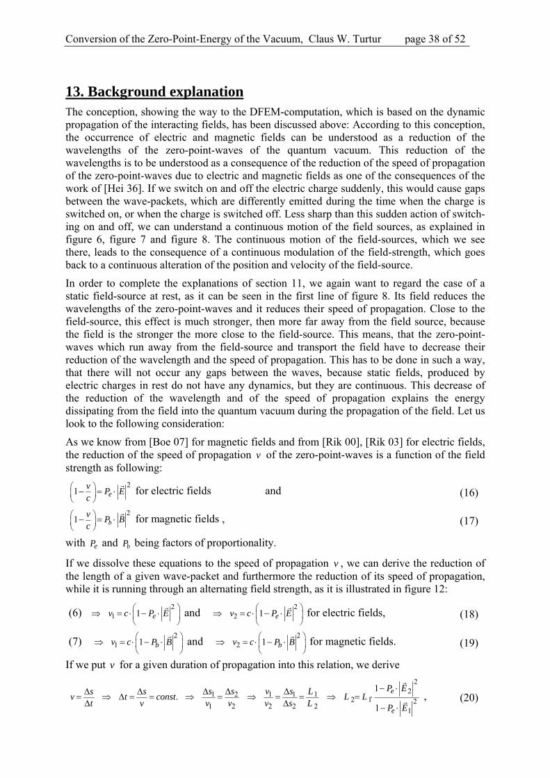
Conversion of the Zero-Point-Energy of the Vacuum, Claus W. Turtur page 38 of 52 xxx
13. Background explanation The conception, showing the way to the DFEM-computation, which is based on the dynamic propagation of the interacting fields, has been discussed above: According to this conception, the occurrence of electric and magnetic fields can be understood as a reduction of the wavelengths of the zero-point-waves of the quantum vacuum. This reduction of the wavelengths is to be understood as a consequence of the reduction of the speed of propagation of the zero-point-waves due to electric and magnetic fields as one of the consequences of the work of [Hei 36]. If we switch on and off the electric charge suddenly, this would cause gaps between the wave-packets, which are differently emitted during the time when the charge is switched on, or when the charge is switched off. Less sharp than this sudden action of switch-ing on and off, we can understand a continuous motion of the field sources, as explained in figure 6, figure 7 and figure 8. The continuous motion of the field-sources, which we see there, leads to the consequence of a continuous modulation of the field-strength, which goes back to a continuous alteration of the position and velocity of the field-source.
In order to complete the explanations of section 11, we again want to regard the case of a static field-source at rest, as it can be seen in the first line of figure 8. Its field reduces the wavelengths of the zero-point-waves and it reduces their speed of propagation. Close to the field-source, this effect is much stronger, then more far away from the field source, because the field is the stronger the more close to the field-source. This means, that the zero-point-waves which run away from the field-source and transport the field have to decrease their reduction of the wavelength and the speed of propagation. This has to be done in such a way, that there will not occur any gaps between the waves, because static fields, produced by electric charges in rest do not have any dynamics, but they are continuous. This decrease of the reduction of the wavelength and of the speed of propagation explains the energy dissipating from the field into the quantum vacuum during the propagation of the field. Let us look to the following consideration:
As we know from [Boe 07] for magnetic fields and from [Rik 00], [Rik 03] for electric fields, the reduction of the speed of propagation v of the zero-point-waves is a function of the field strength as following:
21 e
vP E
c
for electric fields and (16)
21 b
vP B
c
for magnetic fields , (17)
with eP and bP being factors of proportionality.
If we dissolve these equations to the speed of propagation v , we can derive the reduction of the length of a given wave-packet and furthermore the reduction of its speed of propagation, while it is running through an alternating field strength, as it is illustrated in figure 12:
(6)2
1 1 ev c P E
and 2
2 1 ev c P E
for electric fields, (18)
(7) 2
1 1 bv c P B
and 2
2 1 bv c P B
for magnetic fields. (19)
If we put v for a given duration of propagation into this relation, we derive
221 2 1 1 1
2 1 21 2 2 2 2
1
1.
1
e
e
P Es s v s Ls sv t const L L
t v v v v s L P E
, (20)
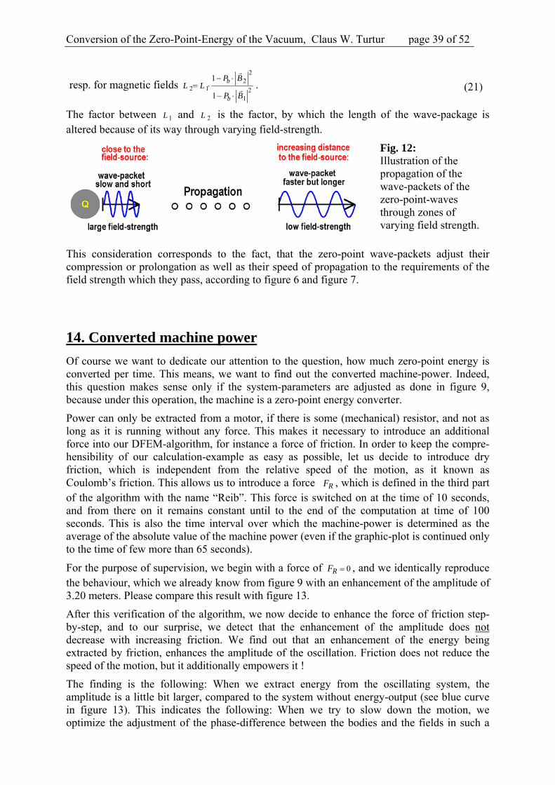
Conversion of the Zero-Point-Energy of the Vacuum, Claus W. Turtur page 39 of 52 xxx
resp. for magnetic fields 2
22 1 2
1
1
1
b
b
P BL L
P B
. (21)
The factor between 1L and 2L is the factor, by which the length of the wave-package is altered because of its way through varying field-strength.
Fig. 12: Illustration of the propagation of the wave-packets of the zero-point-waves through zones of varying field strength.
This consideration corresponds to the fact, that the zero-point wave-packets adjust their compression or prolongation as well as their speed of propagation to the requirements of the field strength which they pass, according to figure 6 and figure 7.
14. Converted machine power
Of course we want to dedicate our attention to the question, how much zero-point energy is converted per time. This means, we want to find out the converted machine-power. Indeed, this question makes sense only if the system-parameters are adjusted as done in figure 9, because under this operation, the machine is a zero-point energy converter.
Power can only be extracted from a motor, if there is some (mechanical) resistor, and not as long as it is running without any force. This makes it necessary to introduce an additional force into our DFEM-algorithm, for instance a force of friction. In order to keep the compre-hensibility of our calculation-example as easy as possible, let us decide to introduce dry friction, which is independent from the relative speed of the motion, as it known as Coulomb’s friction. This allows us to introduce a force RF , which is defined in the third part of the algorithm with the name “Reib”. This force is switched on at the time of 10 seconds, and from there on it remains constant until to the end of the computation at time of 100 seconds. This is also the time interval over which the machine-power is determined as the average of the absolute value of the machine power (even if the graphic-plot is continued only to the time of few more than 65 seconds).
For the purpose of supervision, we begin with a force of 0RF , and we identically reproduce the behaviour, which we already know from figure 9 with an enhancement of the amplitude of 3.20 meters. Please compare this result with figure 13.
After this verification of the algorithm, we now decide to enhance the force of friction step-by-step, and to our surprise, we detect that the enhancement of the amplitude does not decrease with increasing friction. We find out that an enhancement of the energy being extracted by friction, enhances the amplitude of the oscillation. Friction does not reduce the speed of the motion, but it additionally empowers it !
The finding is the following: When we extract energy from the oscillating system, the amplitude is a little bit larger, compared to the system without energy-output (see blue curve in figure 13). This indicates the following: When we try to slow down the motion, we optimize the adjustment of the phase-difference between the bodies and the fields in such a
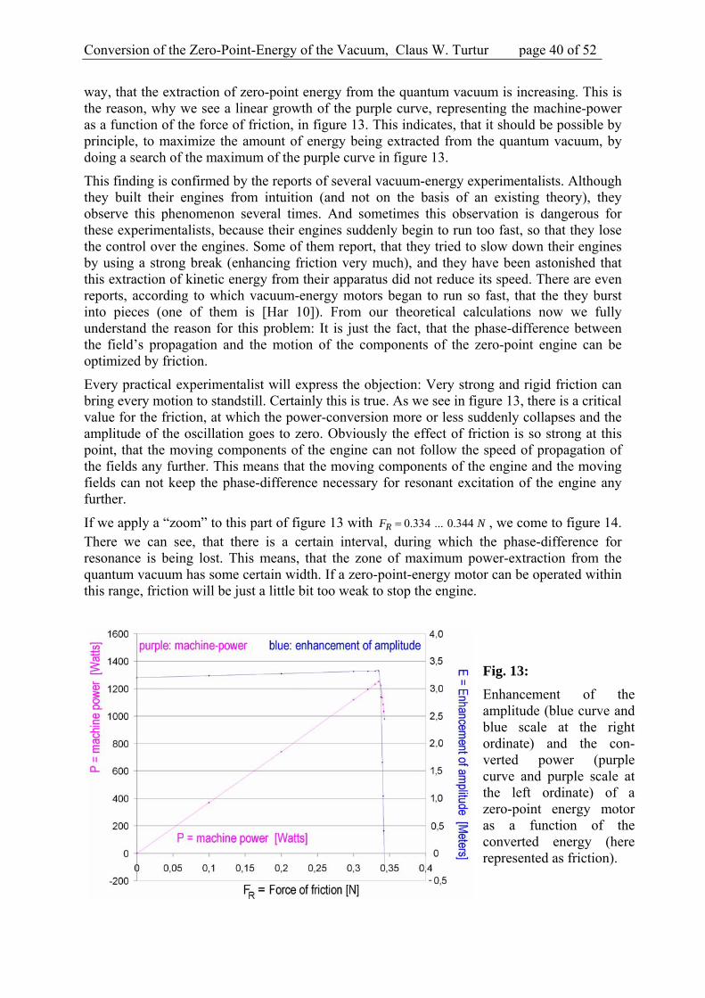
Conversion of the Zero-Point-Energy of the Vacuum, Claus W. Turtur page 40 of 52 xxx
way, that the extraction of zero-point energy from the quantum vacuum is increasing. This is the reason, why we see a linear growth of the purple curve, representing the machine-power as a function of the force of friction, in figure 13. This indicates, that it should be possible by principle, to maximize the amount of energy being extracted from the quantum vacuum, by doing a search of the maximum of the purple curve in figure 13.
This finding is confirmed by the reports of several vacuum-energy experimentalists. Although they built their engines from intuition (and not on the basis of an existing theory), they observe this phenomenon several times. And sometimes this observation is dangerous for these experimentalists, because their engines suddenly begin to run too fast, so that they lose the control over the engines. Some of them report, that they tried to slow down their engines by using a strong break (enhancing friction very much), and they have been astonished that this extraction of kinetic energy from their apparatus did not reduce its speed. There are even reports, according to which vacuum-energy motors began to run so fast, that the they burst into pieces (one of them is [Har 10]). From our theoretical calculations now we fully understand the reason for this problem: It is just the fact, that the phase-difference between the field’s propagation and the motion of the components of the zero-point engine can be optimized by friction.
Every practical experimentalist will express the objection: Very strong and rigid friction can bring every motion to standstill. Certainly this is true. As we see in figure 13, there is a critical value for the friction, at which the power-conversion more or less suddenly collapses and the amplitude of the oscillation goes to zero. Obviously the effect of friction is so strong at this point, that the moving components of the engine can not follow the speed of propagation of the fields any further. This means that the moving components of the engine and the moving fields can not keep the phase-difference necessary for resonant excitation of the engine any further.
If we apply a “zoom” to this part of figure 13 with 0.334 ... 0.344RF N , we come to figure 14. There we can see, that there is a certain interval, during which the phase-difference for resonance is being lost. This means, that the zone of maximum power-extraction from the quantum vacuum has some certain width. If a zero-point-energy motor can be operated within this range, friction will be just a little bit too weak to stop the engine.
Fig. 13:
Enhancement of the amplitude (blue curve and blue scale at the right ordinate) and the con-verted power (purple curve and purple scale at the left ordinate) of a zero-point energy motor as a function of the converted energy (here represented as friction).

Conversion of the Zero-Point-Energy of the Vacuum, Claus W. Turtur page 41 of 52 xxx
Fig. 14:
„Zoom“ to Fig.13 at the range of the power-maxi-mum of a zero-point-energy motor.
By the way, a negative enhancement of the amplitude (blue curve below zero) is under-standable very easy. It indicates, that there friction is so strong, that the amplitude is reduced in comparison to its value at the beginning of the oscillation. If we would continue our DFEM-simulation to a longer time interval, the engine would come to standstill under this operation. Under practical operation is necessary, to drive the machine in a way, that the amplitude will be kept constant over long time interval. This should not be difficult, if the extraction of energy (and power) is kept on the left side apart from the maximum of the purple curve.
15. Further components of the vacuum-energy
With regard to our considerations, that matter can only exist because it is supplied permanently with vacuum-energy (see above), we face the question about the basic existence of matter in a new way: Which is the fundamental essence of nature ? Is it particles (with mass) or waves or both of them ? Which is the substance within space, which gives all matter its existence ? For the photon, the answer is rather easy. It can be found in the standard textbooks for students. The space contains electromagnetic zero-point-waves, which are present in a huge quantity, and if one of them is excited into a excited quantum level, a photon is created. As an example and we can regard the photon of visible light. This is a generally known and very easy explanation for photons. In textbooks we read it as following: The (empty) space contains electromagnetic waves, which are described in the formalism of quantum theory as n , where is the wave-function and n the number of photons. If there
is no photon at all, the state is 0n (also written as 0 ), which describes the empty vacuum.

Conversion of the Zero-Point-Energy of the Vacuum, Claus W. Turtur page 42 of 52 xxx
If there are photons, we write a state with 0n (this is n ). Each of these states contains
energy, namely
12nE n . (22)
For the vacuum without photon, this is the energy
1 10 2 2
0E . (23)
With other words: The textbooks claim that the vacuum without any particles is not empty, but it contains energy, which we call vacuum-energy in this article here. But which type of physical entities are actually oscillating there ? Waves are coupled oscillations, which propagate in an appropriate medium, consisting of many Oscillators. The wave causes many oscillators to oscillate. In the case of electromagnetic waves ( 0 as well as n ), electric and magnetic fields play the role of the
medium for the propagation of the waves. This is what we fined in many textbooks for students ( [Man 93], [Köp 97], [Mes 76/79]). In this sense, we understand the nature of the photons as the zero-point-waves of quantum theory, which are brought into the excited state. But which is the nature of all of these other particles which we know - neutrons, protons, electrons, as well as all these different elementary particles, which we know from elementary particle physics ? And what is the nature of the quarks ? There is one distinct difference between all these particles and the photon. Other than the photon, those particles have a rest mass, whereas the photon never can Come to the rest. (Here would do not want to participate the discussion about the rest mass of neutrino. [Sch 97].) Because electromagnetic waves never come to standstill, also photons can never come to standstill. Other elementary particles obviously differ in nature from electromagnetic waves. Nevertheless they can be described in terms of waves, as we know for instance from the electron in the atomic shell, which is described in terms of a wave in quantum-mechanics. But which type of physical entities are actually oscillating there ? If the electrons is described as a wave, or if neutrons, protons or even complete atoms are described as a waves (atomic beam interference [Lüh 09]) – then there should be something which oscillates, forming a medium which allows the propagation of the wave. We face the question about the nature of the oscillators and about the medium for the propagation of the matter-waves, which we use for the particle-wave-dualism in order to describe elementary particles with rest mass. In the textbooks such waves are called to matter-waves, but I never found a textbook with any information about the nature of the propagation-medium of these waves. All I found, was a formula for the determination of the wavelength of these matter-waves. This formula was the first time given by Louis de Broglie [Str 97], [Mes 76/79] and it says that
hp
, (24)
where 346.626 10h Js is Planck’s elementary quantum of action, p is the impulse of the particle in motion and is the wavelength of the matter-wave. But the lack of the propagation-medium is not the only problem on this conception. A further problem is the fact, that the wave disappears in the moment, when the particle comes to
Conversion of the Zero-Point-Energy of the Vacuum, Claus W. Turtur page 43 of 52 xxx
standstill. As soon as the particle comes to a standstill, its impulse is going to zero, 0p , and thus its wavelength is going to infinity . This conception, which is found in many textbooks for students, is complete nonsense, because it would have the consequence, that every bicycle-driver and every car-driver who reduces his speed, would experience diffraction and interference before coming completely to the standstill. This nonsense can be explained as following: Many of the readers have heard the students-joke, in which the de Broglie-wavelength of a bicycle-driver is being calculated. But as for instance regard a bicycle-driver with a weight of
100m kg and a velocity of 18 5km mh sv , so that the joke can calculate the de Broglie –
wavelength according to 34
366.626 10 1.325 10100 5F m
s
Js mkg
hp
, (25)
The joke now puts the question: Do you know, why the bicycle-driver does not undergo diffraction at the tree or at a traffic light - and do you know, why there is no interference of bicycle-drivers at trees ? The humorous answer is: The de Broglie-wavelength is in the order of magnitude of about
3610 m , which is much smaller than the tree. Diffraction and interference only occur, as long as the wavelength has about the same order of magnitude as the tree. Although the joke sounds really grotesque, it makes clear the problems with de Broglie-formula, for the determination of the wavelength of the bicycle-driver: When the bicycle driver reduces his velocity, his impulse goes down until it reaches 0p . Short before he
comes to the standstill, he passes through an impulse of for instance 332.65 10 mp kgs
,
which leads us to a de Broglie-wavelength of 34
33
6.626 10 252.65 10
Fh Js cmmp kg
s
. (26)
Yes, in reality during the reduction of the velocity, the de Broglie-wavelength increases continuously, and so it passes for sure a value, which perfectly fits into the condition for diffraction and interference of the tree. At least in the case of a collition, the spatial coincidence of bicycle-driver and tree is given, so that the bicycle-driver would never have a chance to undergo a crash, but he would be undergo diffraction. Of course this point of view is totally grotesque. Probably many readers of this article would simply smile when reading these lines. But please be aware, that they smile about the conception of matter-waves as presented in our textbooks for students. This means, that there must be something wrong with the contents, which we teach our students. So we again face the questions: What is the nature of matter-waves ? And how can we describe their medium of propagation ? And there is an additional logical difficulty within this widespread conception of matter-waves: If such matter-waves can really exist, quantum-theory zero-point-oscillations and zero-point-waves for them, as they do for every harmonic oscillation (same as it postulates electromagnetic zero-point-waves). Quantum-theory prohibits the disappearance of oscillations in the ground state 0n by principle, quantum-theory demands at least of energy
of 1 10 2 2
0E for the ground state.
Conversion of the Zero-Point-Energy of the Vacuum, Claus W. Turtur page 44 of 52 xxx
Consequently there should be matter-zero-point-waves in the quantum-vacuum, which exist below the matter-waves, which we use to describe particles and matter. The solution of this problem can be derived from the concept, that elementary particles are matter-waves in the state n , with 1n , which contain the energy
12nE n (27)
according to the quantum level 1n , which is above the ground state at 0n , given by
10 2
0E . (28)
Different elementary particles have different quantum number n , and if we remember, that the very fundamental elementary particles are leptons and quarks, we do not need very many different quantum states n , to describe the complete theory of elementary particle physics. In former centuries, scientists have been used to solve discrepancies in theory. They would probably not have accepted discrepancies like those reported here. In our modern century, scientists are used to accept and ignore such discrepancies, so probably nobody will try to solve the problems. We will now initialize a very first attempt towards this solution. A proposal towards this solution can be adjusted as the concept, to regard every elementary particle as a state n . Let us apply this for the first excited state 1n and calculate its energy
according to
11 2
1E , (29)
which is about one level higher than the ground state 0n .
10 2
0E . (30)
The particle at rest (with the velocity 0v ) then has the energy
1 11 0 2 2
1 0E E . (31)
Thus it's frequency can be determined as 2
21 0
m cm c E E . (32)
For the examples of the electron, of the neutron and of the proton we thus come to the frequencies1:
Electron: 2
207.7634 10ee
m c Hz
Neutron: 2
241.4275 10nn
m c Hz
Proton: 2
241.4255 10pp
m cHz
These are the frequencies for the excitation of the states with regard to the ground state. The ground state itself, this is the vacuum without particles, has exactly half of this energy per each zero-point-matter-wave, and it contains many many of such waves.
1 Diese Frequenzen sind bitte nicht mit den Frequenzen aus Abschnitt 8 zu vermischen. Dort wurde die Frequenz der elektromagnetischen Nullpunktsoszillation berechnet, die dafür benötigt wird, das magnetische Feld des Elektrons zu versorgen. Dies hat nichts mit der Ruhemasse des Elektrons zu tun, welche nach den Ausführungen von Abschnitt 7 eindeutig ohne Zusammenhang mit dem elektrischen oder dem magnetischen Feld des Elektrons zu betrachten ist.
Conversion of the Zero-Point-Energy of the Vacuum, Claus W. Turtur page 45 of 52 xxx
What we can not find out with this fundamental logic is the knowledge about the nature of the propagation of the matter-waves. Perhaps all elementary particles can be described by different states of oscillations within one propagation medium for all matter-waves. Perhaps a Fourier-analysis of wave-packages (as the particles are because of their finite size) can be a good approach. In any case, our conception solves the discrepancy between very different values of the energy-density of the quantum-vacuum, which are nowadays found in literature. According to [Boe 02], in [Tur 09] a derivation of the energy density of the electromagnetic zero-point-waves of the quantum-vacuum was given, leading to an energy density of
4 529
2 3 3.
45 6.007 102
e
el mag
m cE JV m
. (33)
On the other hand, Einstein's thoughts regarding Geometrodynamics (see [Whe 68]) come to total energy density of the quantum-vacuum of
4 2113
2 4 31 2π 2 π2 3.32 1044π PGD P
E c c JV L mL
. (34)
Last but not least, measurements of astrophysics can be quoted (see for instance [e1], [GIU 00], [TEG 02], [EFS 02], [TON 03], [RIE 98]), which come to a density of the ponderable matter M of our universe, leading to an acceleration of the speed of expansion of our universe, which can be measured. From these measurements we know the density of the ponderable matter (and according to the mass-energy-equivalence of its energy) of
3 326 2 10(1.0 0.3) 10 9.0 0.27 10kg J
gravM Mm mc . (35)
Please regard the following explanations: The value of (33) gives the energy-density of the electromagnetic zero-point-waves of the quantum vacuum, and can be understood in connection with the propagation of electrostatic and magnetostatic fields as well. The value of (34) has the same goal, but differently from (33) it is based on pure theory, whereas (33) is based on measurements. The problem of the approach (34) is an improper integral, without a clear solution of its convergence problems, which goes back to the integration of infinitely many zero-point-waves with an infinite range of wavelength (see [Whe 68] and [Tur 09]). Very different from those both approaches is (35), which regards only the effect of gravitation due to the ponderable mass in connection with the energy of the vacuum. Consequently the value of (35) must be remarkably smaller than the values, because the energy density of the field of gravitation is not very high. Clear is (and this was also pointed out in [Tur 09]), that the value of (33) only takes the electromagnetic zero-point-oscillations into account, and not know of all the other things, which additionally exist inside the quantum-vacuum, such as for instance matter-waves. The total energy density of the quantum-vacuum, taking all its contents into account, has still to be found. After these thoughts - let us come back to all question about the fundamental essence of nature ? Is it particles (with mass) or waves or both of them ?

Conversion of the Zero-Point-Energy of the Vacuum, Claus W. Turtur page 46 of 52 xxx
From the preceding sections of this work, we remember, that the electrical charge (as for instance the electron) as well as all the ponderable masses (due to the fact that they participate in gravitation) can only exist, because they are supported with energy from the zero-point-waves from the quantum vacuum. This means that the zero-point-waves are the fundamental physical entities which make the existence of all these things possible. So it should be the zero-point-waves, i.e. the vacuum-energy, which define the basis of our world. This logical consideration leads us to the final consequence, that all things within our universe, originate from vacuum-energy, and zero-point-waves. Thus we recognize the vacuum-energy as the real fundament for existence at all. Not matter, but zero-point-waves define everything which we observe in our world. As soon as these zero-point-waves are excited with regard to the ground state, we notice them in the shape of matter:
- Electromagnetic zero-point-waves 0EM
can be excited by one quantum level to
become photons 1EM
.
- Matter zero-point-waves 0G
can be excited analogously by one quantum level to
become elementary particles 1G
.
This means, that matter, same as light, is nothing else than excited zero-point-waves (electromagnetic zero-point-waves respectively matter zero-point-waves). From there we understand the mass-energy-equivalence 2E mc just as an excitation of the energy levels of the zero-point-waves:
- When a photon, thermal radiation, or an electromagnetic wave is absorbed, the zero-point-wave goes from the state 1
EM down to the state 0
EM, and leaves back the
energy 1E . - When a photon, thermal radiation, or an electromagnetic wave is produced, the energy
1E has to be spent, in order to excite the zero-point-wave from the state 0EM
to the state 1EM
.
- When matter is converted into energy (as for instance during classical energy production), matter is lost. The particles which are lost represent zero-point-wave going down from the state 1
G to the ground state 0
G.
- Also the chemical bonding, as it is usual for chemical reactions for energy production, does the same. The only difference is, that the energy is taken from the chemical bonding, which goes back to the electric and magnetic fields within the molecules, keeping the atoms together to the molecule. Combusting matter thus finally goes back to Coulomb-interaction, and the alteration of the energy stored within the Coulomb-field inside the molecules, have influence on the wavelengths of the electromagnetic zero-point-waves within the geometrical range of these fields. This means that chemical reactions take energy from there, that it zero point waves, which penetrate the bonding-zone inside the molecules, in the very last consequence.
- If energy is converted into matter (as we observe it in accelerators, if they are used for experiments of elementary particle physics), zero-point-matter-waves are excited from the state 0
G into another state, as for instance 1
G. The energy, which is necessary
for this reaction, is normally taken from the kinetic energy of the elementary particles within the accelerator-engine. It can be supplied in form of an electromagnetic wave, as for instance when we do pair-production, where a photon decays into an electron-
Conversion of the Zero-Point-Energy of the Vacuum, Claus W. Turtur page 47 of 52 xxx
positron-pair. In this case, the electromagnetic zero-point-wave of the photon 1EM
goes down to the ground state 0EM
a gives its energy to a zero-point-matter-wave,
which is excited from 0EM
up to 1EM
.
All of these examples are working well within energy-transfer according to the conservation of classical energy of the excited states. There is no energy exchange with the zero-point-waves of the quantum vacuum in these examples. Something totally different happens, when the energy of the zero-point-waves of the quantum vacuum are included into the energy-conservation, as it is for instance the case, when we drive a vacuum-energy motor. In this case we extract energy directly from the zero-point-waves of the quantum vacuum, as can be understood in the preceding sections of this article. Of course, energy-conservation is then to be applied to the total energy, which now is the sum of classical energy and zero-point-energy. How can we tap the zero-point-energy of the quantum vacuum ? This is explained for the case of electromagnetic zero-point-waves in preceding sections. But also some few machines are reported worldwide, which are said to be capable, to do this conversion practically [Jeb 06]. In principle, it might be imaginable, that one day it will be possible to exchange energy not only with the electromagnetic zero-point-waves, but also with the zero-point-matter-waves. But there is a principal difference between those both types of zero-point-waves: Electromagnetic zero-point-waves 1
EM can be produced easily without
leaving a hole in the ground state 0EM
, whereas zero-point-matter-waves 1G
leave a hole
in the ground state 0G
, which we normally call antimatter. This has the consequence, that
the energy circulation of the electric and magnetic fields (as it is described above) can not be applied to an analogous circulation of zero-point-matter-waves. We a rather know the effects of “vacuum-polarization” from quantum-electrodynamics, which tell us that zero-point-matter-waves 1
G decay back into the ground state 0
G and thus form of energy circulation
on their own, which is very different from the energy circulation of the electric and magnetic fields. If it would become possible one day, to develop a method for the excitation of zero-point-matter-waves, which would mean the origination of new matter from the quantum-vacuum, it must be a totally different method, than the method which we know for the extraction of electromagnetic zero-point-waves from the quantum-vacuum. The way for this type of interaction with zero-point-matter-waves is not seen today. But as soon as we understand, that not matter is the fundament of our world, but zero-point-energy, we can begin our way towards this fantastic interaction with the zero-point-matter-waves of the quantum-vacuum.

Conversion of the Zero-Point-Energy of the Vacuum, Claus W. Turtur page 48 of 52 xxx
16. Resumée The present work describes the mechanism of the conversion of the zero-point-energy of the quantum-vacuum into classical energy (back and forth). The philosophical principle of this mechanism can be understood, when we regard the energy of the zero-point-oscillations and the zero-point-waves of the quantum-vacuum as the fundamental entity of the universe. This means that we understand photons, elementary particles and ponderable masses as excited zero-point-waves.
Independent from this concept, the computation principle of the zero-point-energy converters is philosophically rather simple. But apart from the philosophical simplicity, the expenditure for the practical computation of the zero-point-energy converters is a rather large:
The computation principle was introduced under the name “Dynamic Finite-Element-Method“ (DFEM), which differs from the classical „Finite-Element-Method“ (FEM) only by the speed of the interactions between the bodies of which a machine consists. And classical FEM, the interaction propagates from one body to each other instantaneously, i.d. with infinite speed. For classical engines, this is a rather good approximation, but for zero-point-energy converters, this approximation is too rough. The computation of zero-point-energy motors requires, that we take the finite speed of propagation of the interacting fields (which is not faster than the speed of light) into account.
17. Literature-References [Alm 09] GEET-Reaktor by Paul Pantone
http://www.science-explorer.de/plasmareaktor.htm Successful further development by Theo Almeida-Murphy,
presented at the conference „Neue Energie-Technologien“ by Adolf and Inge Schneider, Bruchsal, Sept. 2009
[Ans 08] Finite Elemente Programm ANSYS, John Swanson (1970-2008)
ANSYS, Inc. Software Products, http://www.ansys.com [Bea 02] Motionless Electromagnetic Generator, Tom Bearden et. al.
US Patent, 6,362,718 from 26. März 2002 Inventors: Patrick L. Stephen, Thomas E. Bearden, James C. Hayes, Kenneth D. Moore, James L. Kenny To be found at http://www.cheniere.org/
[Bec 73] Theorie der Elektrizität, Richard Becker and Fritz Sauter
Teubner Verlag. 1973. ISBN 3-519-23006-2 [Ber 71] Bergmann-Schaefer, Lehrbuch der Experimentalphysik H.Gobrecht, Verlag Walter de Gruyter, 1971, ISBN 3-11-002090-0 [Bia 70] Nonlinear Effects in Quantum Electrodynamics. Photon Propagation and Photon Splitting in
an external Field, Z.Bialynicka-Birula und I.Bialynicki-Birula Phys. Rev. D. 1970, Vol.2, No.10, page 2341

Conversion of the Zero-Point-Energy of the Vacuum, Claus W. Turtur page 49 of 52 xxx
[Boe 07] Exploring the QED vacuum with laser interferometers Daniël Boer und Jan-Willem van Holten, arXiv:hep-ph/0204207v1,
several versions from 17. April 2002 until to 1. Feb. 2008 [Bor 99] Borland Pascal (Delphi 5 aus 1999 oder neuere Version) [Boy 66..08] Timothy H. Boyer has a huge list of publications (Am. J. Phys., Il Nuovo Cimento,
Ann. Phys., Phys. Rev., J. Math. Phys., Found. Phys. and many others), which begins in 1966 and goes up to 2008. It is to be found at http://www.sci.ccny.cuny.edu/physics/faculty/boyer.htm For many well-known phenomena in quantum theory there are alternative derivations in the framework of stochastic electrodynamics, completely without the use of any quantum theory.
[Boy 80] A Brief Survey of Stochastic Electrodynamics, by Timothy Boyer Foundation of Radiation Theory and Quantum Electrodynamics Editor: A. O. Barut, Plenum, New York 1980. [Boy 85] The Classical Vacuum by Timothy Boyer Scientific American 253, No.2, August 1985, p.70 -78 [Bro 10] Brown's Gas, George Wiseman
To be found at www.eagle-research.com or http://www.browns-gas.de/ [Cal 84..09] Calphysics Institute (Director Bernard Haisch)
There is an extensive list of publications (Ann. Phys., Phys. Rev., Found. Phys. and many others), beginning in 1984 and going until today. It can be found at:
http://www.calphysics.org/index.html [Cas 48] On the attraction between two perfectly conducting plates.
H. B. G. Casimir (1948), Proceedings of the Section of Sciences Koninklijke Nederlandse Akademie van Wetenschappen, S.795 As well as H. B. G. Casimir and D. Polder, Phys. Rev. 73 (1948) S. 360
[Cel 07] The Accelerated Expansion of the Universe Challenged by an Effect of the Inhomogeneities.
A Review, Marie-Noëlle Célérier, arXiv:astro-ph/0702416 v2, 7. Jun. 2007 [Cod 00] CODATA Recommended Values of the Fundamental Physical Constants: 1998 Review of Modern Physics 72 (2) 351 (April 2000)
The contents of CODATA are updated continuously at: http://physics.nist.gov/cuu/Constants/
[Der 56] Direct measurement of molecular attraction between solids separated by a narrow gap ,
Boris V. Derjaguin, I. I. Abrikosowa, Jewgeni M. Lifschitz Q. Rev. Chem. Soc. 10, 295–329 (1956) Springer Verlag. 2006. ISBN 3-540-33794-6
[Dob 03] Physik für Ingenieure, 10.Aufl., Dez. 2003 Paul Dobrinski, Gunter Krakau, Anselm Vogel, ISBN 3-519-46501-9 [Efs 02] The Monthly Notices of the Royal Astronomical Society
George Efstathiou, Volume 330, No. 2, 21. Feb. 2002 [Fey 49a] The Theory of Positrons, Richard P. Feynman Phys. Rev. 76, No.6 (1949), p.749-759

Conversion of the Zero-Point-Energy of the Vacuum, Claus W. Turtur page 50 of 52 xxx
[Fey 49b] Space-Time Approach to Quantum Electrodynamics, Richard P. Feynman Phys. Rev. 76, No.6 (1949), p.769-789 [Fey 85] QED. Die seltsame Theorie des Lichts und der Materie, Richard P. Feynman
Translated reprint of 1985, Serie Piper, ISBN: 3-492-03103-X [Fey 97] Quantenelektrodynamik: Eine Vorlesungsmitschrift, Richard P. Feynman German translation at Oldenbourg Verlag. 1997. ISBN 3-486-24337-3 [Fey 01] Feynman Vorlesungen über Physik, Band II: Elektromagnetismus und Struktur der Materie,
Richard P. Feynman, Robert B. Leighton and Matthew Sands Oldenbourg Verlag, 3.Auflage. 2001. ISBN 3-486-25589-4
[Giu 00] Das Rätsel der kosmologischen Vakuumenergiedichte und die beschleunigte Expansion des
Universums, Domenico Giulini and Norbert Straumann arXiv:astro-ph/0009368 v1, 22. Sept. 2000
[Goe 96] Einführung in die Spezielle und Allgemeine Relativitätstheorie, Hubert Goenner
Spektrum Akademischer Verlag, 1996. ISBN 3-86025-333-6 [Gpb 07] Gravity- Probe- B Experiment, Francis Everitt et. al.
To be found (2008) at http://einstein.stanford.edu/index.html [Har 10] Example by Guy Hary at the Congress „Autonome Energiesysteme“, 3.-5. Sept. 2010
at Schloss Hofen in Lochau near Bregenz; Schweizerische Vereinigung für Raumenergie SVR, Jupiter-Verlag/TransAltec AG, Zürich
[Hei 36] Folgerungen aus der Diracschen Theorie des Positrons W. Heisenberg und H. Euler, 22.Dez.1935, Zeitschrift für Physik (1936), S.714 [Hil 96] Elementare Teilchenphysik, Helmut Hilscher
Vieweg Verlag, ISBN 3-528-06670-9 [Hur 40] The Invention of Hans Coler, Relating To An Alleged New Source Of Power.
R. Hurst, B.I.O.S. Final Report No. 1043, B.I.O.S.Trip No. 2394 B.I.O.S. Target Number: C31/4799, British Intelligence Objectives Sub-Committee
[Jac 81] Klassische Elektrodynamik, John David Jackson
Walter de Gruyter Verlag. 1981. ISBN 3-11-007415-X [Jeb 06] Die Urkraft aus dem Universum, Klaus Jebens
Jupiter-Verlag. 2006. ISBN 3-906571-23-8 [Köp 97] Einführung in die Quanten - Elektrodynamik
G.Köpp und F.Krüger B.G.Teubner Verlag, Stuttgart 1997, ISBN 3-519-03235-X
[Lam 97] Demonstration of the Casimir force in the 0.6 to 6 µm range Steve K. Lamoreaux, Phys. Rev. Lett., Vol.78, Issue 1, Jan-6-1997, p.5-8
DOI: 10.1103/PhysRevLett.78.5 [Lif 56] The theory of molecular attractive forces between solids. Jewgeni M. Lifschitz, Sov. Phys. JETP 2, 73–83 (1956) [Loh 05] Hochenergiephysik, Erich Lohrmann
Teubner Verlag. 2005. ISBN 3-519-43043-6

Conversion of the Zero-Point-Energy of the Vacuum, Claus W. Turtur page 51 of 52 xxx
[Lüh 09] Quantenphysik in der Nanowelt: Schrödingers Katze bei den Zwergen
Hans Lüth, Springer-Verlag, 2009, ISBN 978-3-540-71043-1 [Man 93] Quantenfeldtheorie, Franz Mandl und Graham Shaw
Aula-Verlag, Wiesbaden. 1993. ISBN 3-89104-532-8 [Mar 88-98] ▪ Der Kugellager-Motor und der Huber-Effekt,
Stefan Marinov, raum&zeit 32 (1988) 81-84 ▪ Repetition of Silvertooth's experiment for measuring the aether drift",
Stefan Marinov, Speculations in Science and Technology 12 No.3 (1989) 187-179 ▪ Propulsive and Rotating Ampère Bridges and the Principle of Relativity Stefan Marinov, Physics Essays 4 No.1 (1991) 30-36 ▪ The Missing Magnetic Force Law, Galilean Electrodynamics 9 No.2 Stefan Marinov, (March/April 1998) 35-37
[Mes 76/79] Quantenmechanik, Bände 1 + 2, Albert Messiah, Walter de Gruyter Verlag ISBN 3-11-003686-X (Band 1, 1976) and ISBN 3-11-003687-8 (Band 2, 1979) [Mie 84] Kompendium Hypertechnik. Tachyonenenergie, Hyperenergie, Antigravitation.
Sven Mielordt, Berlin, 1984 Nachdruck der 4. Auflage vom raum&zeit Verlag, ISBN 3-89005-005-0
[Nag 10] private communication, Paul Nagy and Christian Preinfalk, Sept. 2010 [Nie 83] Konversion von Schwerkraft-Feld-Energie. Revolution in Technik, Medizin, Gesellschaft.
Von Hans A. Nieper MIT-Verlag, Oldenburg, 1983, 4. erw. Auflage, ISBN 3-925188-00-2
[Pau 00] Relativitätstheorie, Wolfgang Pauli Nachdruck im Springer-Verlag, 2000. ISBN 3-540-67312-1 [Pau 10] Online Skript „Teilchen und Kerne“ by S. Paul und W. Weise Physik-Department der TU-München, 2010
http://www.e18.physik.tu-muenchen.de/skript/index.html [Rie 98] Observational Evidence from Supernovae for an Accelerating Universe and a Cosmological
Constant, Adam G. Riess et. al. arXiv:astro-ph/9805201, 15. Mai. 1998
[Rik 00] Magnetoelectric birefringences of the quantum vacuum
G. L. J. A. Rikken and C. Rizzo, 2000, Phys. Rev. A, Vol.63, 012107 (2000)
[Rik 03] Magnetoelectric anisotropy of the quantum vacuum G. L. J. A. Rikken and C. Rizzo, 2003, Phys. Rev. A, Vol.67, 015801 (2003)
[Ruz 09] Ein praktischer Nachweis der Dunklen Energie
Claus W. Turtur, Raum&Zeit, 2.Jahrgang, Heft 2, Oktober 2009, S.67
[Sch 97] Neutrinophysik, von Norbert Schmitz, Teubner Studienbücher ISBN: 3-519-03236-8 , Erschienen: Juni 1997 [Sch 02] Gravitation, Ulrich E. Schröder
Verlag Harri Deutsch, 2002. ISBN 3-8171-1679-9

Conversion of the Zero-Point-Energy of the Vacuum, Claus W. Turtur page 52 of 52 xxx
[Sch 10] Congress „Autonome Energiesysteme“, NET-Journal, Jg.Nr. 15, Heft 7/8, Juli/Aug.2010 Jupiter Verlag, Adolf and Inge Schneider, ISSN 1420-9292 The series of “NET-Journals” deals since many years with the utilization of vacuum-energy. [Sim 80] Absolute electron-proton cross sections at low momentum transfer measured with
a high pressure gas target system G.G.Simon, Ch.Schmitt, F.Borkowski, V.H.Walther Nucl. Phys. A, vol.333, issue 3, (1980), p.381-391
[Spa 58] Measurement of attractive forces between flat plates.
Marcus J. Spaarnay, Physica. Band 24, 1958, S. 751. [Str 97] Quantenmechanik: Ein Grundkurs über nichtrelativistische Quantentheorie
Norbert Straumann, Springer-Verlag, ISBN 3-54042888-7 [Stu 06] Kurzes Lehrbuch der Physik
Herbert A. Stuart, Gerhard Klages Springer-Verlag, 18. Auflage, 2006, ISBN 978-3-540-23146-2
[Teg 02] Measuring Spacetime: from Big Bang to Black Holes Max Tegmark, arXiv:astro-ph/0207199 v1, 10. Juli 2002 Slightly abbreviated version in: Science, 296, 1427-1433 (2002) [Thi 18] Über die Wirkung rotierender ferner Massen in Einsteins Gravitationstheorie Hans Thirring und Josef Lense, Phys. Zeitschr. 19, Seiten 33-39 Jahrgang 1918 [Ton 03] Cosmological Results from High-z Supernovae John L. Tonry, et. al., arXiv:astro-ph/0305008, 1. Mai 2003 [Tur 07a] Two Paradoxes of the Existence of electric Charge
Claus W. Turtur, arXiv:physics/0710.3253 v1 (Okt.2007) [Tur 07b] Two Paradoxes of the Existence of magnetic Fields, Claus W. Turtur
PHILICA.COM, ISSN 1751-3030, Article number 113, (19. December 2007) [Tur 08] A QED-model for the Energy of the Vacuum and an Explanation of its Conversion into
Mechanical Energy, Claus W. Turtur PHILICA.COM, ISSN 1751-3030, Article number 138, (4. Sept. 2008)
[Tur 09] Wandlung von Vakuumenergie elektromagnetischer Nullpunktsoszillationen in klassische
mechanische Energie, Claus W. Turtur, 1. Auflage 2009, Europäischer Hochschuleverlag, ISBN 978-3-941482-54-8
Conversion of the Zero-point Energy of the Quantum Vacuum into Classical Mechanical Energy, Claus W. Turtur, 1. Auflage 2009, Europäischer Hochschuleverlag, ISBN 978-3-941482-60-9
[Val 08] Zero Point Energy, The fuel of the future
Thomas Valone, Integrity Research Institute, 2008. ISBN 978-0-9641070-2-1 [Wik 10] Higgs-Mechanismus, Wikipedia
http://de.wikipedia.org/wiki/Higgs-Mechanismus [Whe 68] Einsteins Vision Wie steht es heute mit Einsteins Vision, alles als Geometrie aufzufassen ? John Archibald Wheeler. 1968. Springer Verlag