Embed Size (px)
Citation preview
Fundamental Analysis and the Cross-Sectionof Stock Returns: A Data-Mining Approach
Xuemin (Sterling) YanUniversity of Missouri
Lingling ZhengRenmin University of China
We construct a “universe” of over 18,000 fundamental signals from financial statementsand use a bootstrap approach to evaluate the impact of data mining on fundamental-basedanomalies. We find that many fundamental signals are significant predictors of cross-sectional stock returns even after accounting for data mining. This predictive ability ismore pronounced following high-sentiment periods and among stocks with greater limitsto arbitrage. Our evidence suggests that fundamental-based anomalies, including thosenewly discovered in this study, cannot be attributed to random chance, and they are betterexplained by mispricing. Our approach is general and we also apply it to past return–basedanomalies. (JEL G12, G14)
Received October 22, 2015; editorial decision October 27, 2016 by Editor Andrew Karolyi.
Economists place a premium on the discovery of puzzles, whichin the context at hand amounts to finding apparent rejections of awidely accepted theory of stock market behavior.
—Merton (1987, 104)
Finance researchers have devoted a considerable amount of time and effortto searching for stock return patterns that cannot be explained by traditionalasset pricing models. As a result of these efforts, there is now a largebody of literature documenting hundreds of cross-sectional return anomalies
Xuemin (Sterling) Yan is with the Robert J. Trulaske Sr. College of Business, University of Missouri, Columbia,MO. Lingling Zheng is with the School of Business, Renmin University of China, Beijing, China. We thankPedro Barroso, Honghui Chen, Jere Francis, Jennifer Huang, Xin Huang, Wenxi Jiang, Andrew Karolyi (theeditor), Inder Khurana, Dong Lou, Haitao Mo, Chenkai Ni, Reynolde Pereira, Riccardo Sabbatucci, XuepingWu, Chengxi Yin, an anonymous referee, and seminar participants at Cheung Kong Graduate School ofBusiness, CICF 2016, City University of Hong Kong, EFA 2016, FMA European Conference 2016, Hong KongPolytechnic University, Louisiana State University, Renmin University of China, SGF 2016 Annual Conference,Tsinghua University, University of Central Florida, and University of Missouri for helpful comments. Weacknowledge financial support from Renmin University of China (Project No. 16XNKI006). Supplementarydata can be found on The Review of Financial Studies web site. Send correspondence to Lingling Zheng at theSchool of Business, Renmin University of China, Beijing, 100872, China; telephone: 86-10-82500431. E-mail:[email protected].
© The Author 2017. Published by Oxford University Press on behalf of The Society for Financial Studies.All rights reserved. For Permissions, please e-mail: [email protected]:10.1093/rfs/hhx001 Advance Access publication March 6, 2017
Dow
nloaded from https://academ
ic.oup.com/rfs/article-abstract/30/4/1382/2908895 by R
enmin U
niversity user on 13 Novem
ber 2019
Fundamental Analysis and the Cross-Section of Stock Returns
(Green, Hand, and Zhang 2013, 2014; Harvey, Liu, and Zhu 2016; McLean andPontiff 2016). An important debate in the literature is whether the abnormalreturns documented in these studies are compensation for systematic risk,evidence of market inefficiency, or simply the result of extensive data mining.
Data-mining concern arises because “the more scrutiny a collection of datais subjected to, the more likely will interesting (spurious) patterns emerge” (Loand Mackinlay 1990, 432). Intuitively, if enough variables are considered, thenby pure chance some of these variables will generate abnormal returns even ifthey do not genuinely have any predictive ability for future stock returns. Loand MacKinlay contend that the degree of data mining bias increases with thenumber of studies published on the topic. The cross-section of stock returns isarguably the most researched and published topic in finance; hence, the potentialfor spurious findings is also the greatest.
Although researchers have long recognized the potential danger of datamining, few studies have examined its impact on a broad set of cross-sectionalstock return anomalies.1 The lack of research in this area is in part because ofthe difficulty to account for all the anomaly variables that have been consideredby researchers. Although one can easily identify published variables, onecannot observe the numerous variables that have been tried but not publishedor reported due to the “publication bias.”2 In this paper, we overcome thischallenge by examining a large and important class of anomaly variablesthat are derived from financial statements (what we call “fundamental-basedvariables”), for which a “universe” can be reasonably constructed.
We focus on fundamental-based variables for several reasons. First, manyprominent anomalies such as the asset growth anomaly (Cooper, Gulen, andSchill 2008) and the gross profitability anomaly (Novy-Marx 2013) are basedon financial statement variables. Harvey, Liu, and Zhu (2016) report thataccounting variables represent the largest group among all the published cross-sectional return predictors. Second, researchers have considerable discretionto the selection and construction of fundamental signals. As such, there isample opportunity for data snooping. Third and most importantly, althoughthere are hundreds of financial statement variables and numerous ways ofcombining them, we can construct a “universe” of fundamental signals byusing permutational arguments. The ability to construct such a universe isimportant because in order to account for the effect of data mining, one shouldnot only include variables that were reported, but also variables that wereconsidered but unreported (Sullivan, Timmermann, and White 1999, 2001).Financial statement variables are ideally suited for such an analysis.
We construct a universe of fundamental signals by imitating the searchprocess of a data snooper. We start with all accounting variables in Compustat
1 The exceptions are Harvey, Liu, and Zhu (2016) and McLean and Pontiff (2016).
2 The publication bias refers to the fact that it is difficult to publish a nonresult (Harvey, Liu, and Zhu 2016).
1383
Dow
nloaded from https://academ
ic.oup.com/rfs/article-abstract/30/4/1382/2908895 by R
enmin U
niversity user on 13 Novem
ber 2019
The Review of Financial Studies / v 30 n 4 2017
and then impose a minimum amount of data requirement, which leads to atotal of 240 accounting variables. For each variable, we consider 76 financialratio configurations. By using permutational arguments (i.e., including allcombinations of accounting variables and financial ratio configurations), wethen construct a universe of over 18,000 fundamental signals.
We form long-short portfolios based on each fundamental signal and assessthe significance of long-short returns by using a bootstrap procedure. Thebootstrap is a nonparametric method for estimating the distribution of anestimator or test statistic by resampling one’s data (Horowitz 2001). Thebootstrap approach is desirable in our context for several reasons. First,long-short returns are highly non-normal. Second, long-short returns acrossfundamental signals exhibit complex cross-sectional dependencies. Third,evaluating the performance of a large number of fundamental signals involvesa multiple comparison problem (Harvey, Liu, and Zhu 2016).
We follow Fama and French (2010) and randomly sample time periods withreplacement. That is, we draw the entire cross-section of long-short returnsfor each time period. The simulated returns have the same properties as theactual returns except that we set the true alpha for the simulated returns to zero.We estimate alphas relative to the CAPM, the Fama and French three-factormodel, and the Carhart four-factor model. We follow Kosowski et al. (2006)and conduct our bootstrap analysis on both alphas and the t-statistics of alphas.By comparing the cross-sectional distribution of actual alphas (t-statistics) tothe distribution of alphas (t-statistics) from the simulated samples, we are ableto assess the extent to which the observed performance of top-ranked signalsis due to sampling variation (i.e., random chance).
Our results indicate that the top-ranked fundamental signals in our sampleexhibit superior long-short performance that is not due to sampling variation.The bootstrapped p-values for the extreme percentiles of alphas are generallyless than 5%. For example, the 99th percentile of equal-weighted three-factoralphas is 0.84% per month in the actual data, with a bootstrapped p-valueof 1.1%, indicating that only 1.1% of the simulation runs produce a 99thpercentile of alphas higher than 0.84%. The results for t-statistics are evenmore significant. For example, the 99th percentile of t-statistics for equal-weighted three-factor alphas is 4.82 in the actual data. In comparison, noneof the simulation runs generate a 99th percentile of t-statistics that is as highas 4.82. In other words, we would not expect to find such extreme t-statisticsunder the null hypothesis of no predictive ability. The results for value-weightedreturns are qualitatively similar. For example, the 99th percentile of three-factoralpha t-statistics is 3.66 in the actual data, with a bootstrapped p-value of 0%.Overall, our bootstrap results suggest that the superior performance of the topfundamental signals cannot be attributed to pure chance.
Our results are robust to alternative universe of fundamental signals,alternative sampling procedure, and alternative benchmark models includingthe Fama and French (2015) five-factor model. In addition, we find qualitatively
1384
Dow
nloaded from https://academ
ic.oup.com/rfs/article-abstract/30/4/1382/2908895 by R
enmin U
niversity user on 13 Novem
ber 2019
Fundamental Analysis and the Cross-Section of Stock Returns
the same results whether we exclude or include financial stocks. Finally, ourresults are unchanged when we use industry-adjusted fundamental signals.
Having shown that fundamental-based anomalies are not due to randomchance, we next investigate whether they are consistent with mispricing- orrisk-based explanations. We conduct three tests. First, behavioral argumentssuggest that if the abnormal returns to fundamental-based trading strategiesarise from mispricing, then they should be stronger among stocks with greaterlimits to arbitrage (Shleifer and Vishny 1997). Consistent with this prediction,we find that the predictive ability of top fundamental signals is more pronouncedamong small, low-institutional ownership, high-idiosyncratic volatility, andlow-analyst coverage stocks. Second, to the extent that fundamental-basedanomalies are driven by mispricing, anomaly returns should be significantlyhigher following high-sentiment periods (Stambaugh, Yu, and Yuan 2012). Wefind strong evidence consistent with this prediction. Third, we examine whetheranomaly returns vary across the business cycle (Chordia and Shivakumar2002). If the superior performance of top fundamental signals representscompensation for systematic risk, then we should expect the anomaly returns tobe significantly lower during bad times (when the marginal utility of wealth ishigh) than during good times (Cochrane 2004). Contrary to this prediction, wefind that the long-short returns of top fundamental signals are actually higherduring recessions than during expansions, although the difference is statisticallyinsignificant. Taken together, although we cannot completely rule out risk-based explanations, our evidence suggests that fundamental-based anomaliesare more consistent with mispricing-based explanations.
Our results indicate that a large number of fundamental signals exhibitgenuine predictive ability for future stock returns. While some of these signalshave been explored by previous studies, many of the top fundamental signalsidentified in this study are new and have received little direct attention inthe prior literature. For example, we find that anomaly variables constructedbased on interest expense, tax loss carryforward, and selling, general, andadministrative expense are highly correlated with future stock returns. Broadlyspeaking, these variables may predict future stock returns because they containvalue-relevant information about future firm performance and the market failsto incorporate this information into stock prices in a timely manner. Tradingcost cannot fully explain the delayed reaction to public accounting informationbecause the trading strategies considered in our study are rebalanced once ayear and have low turnover rates. We argue that limited attention is a moreplausible reason why investors fail to fully appreciate the information contentof the fundamental variables documented in this study.
A key innovation of our paper is to construct a universe of fundamentalsignals. Although we focus on financial statement variables in this paper, ourapproach is general and can be applied to other categories of anomaly variables.We demonstrate this generality by applying our methodology to past return–based anomalies. Previous studies have shown that short-, intermediate-, and
1385
Dow
nloaded from https://academ
ic.oup.com/rfs/article-abstract/30/4/1382/2908895 by R
enmin U
niversity user on 13 Novem
ber 2019

The Review of Financial Studies / v 30 n 4 2017
long-horizon past returns contain significant information about future stockreturns (DeBondt and Thaler 1985; Jegadeesh 1990; and Jegadeesh and Titman1993). More recently, Novy-Marx (2012) shows that the momentum effect isprimarily driven by stock returns during twelve to seven months prior to theportfolio formation date, and Heston and Sadka (2008) document that past stockreturns have significant predictive power for future returns of the same calendarmonth. We evaluate the extent to which these past return–based anomalies ariseby pure chance.
Similar to financial statement variables, past return variables are also wellsuited for our analysis because although researchers have numerous choices onwhich past returns to use, we can construct a “universe” of past return signalsby using permutational arguments. Our bootstrap results based on 4,080 pastreturn signals indicate that the predictive ability of intermediate-horizon returns(i.e., the momentum effect) cannot be explained by random chance. However,the predictability of long-run past returns (i.e., the long-run reversal effect) issensitive to the benchmark model and the portfolio weighting scheme.
Our study adds to an emerging literature on meta-analysis of marketanomalies. The closest paper to ours is Harvey, Liu, and Zhu (2016), who usestandard multiple-testing methods to correct for data mining in 315 publishedreturn predictors. Standard multiple-testing methods, however, cannot accountfor the exact cross-sectional dependency in test statistics. Moreover, becauseunpublished factors are unobservable Harvey, Liu, and Zhu have to makeassumptions about the fraction of the unobserved tests. Our paper differs fromHarvey, Liu, and Zhu in that we explicitly construct a universe of anomalyvariables and we use a bootstrap procedure to evaluate data mining. Anotherrelated paper is McLean and Pontiff (2016), who use an out-of-sample approachto evaluate data-mining bias in market anomalies. They examine the post-publication performance of ninety-seven anomalies and document an averageperformance decline of 58%. Green, Hand, and Zhang (2013, 2014) examinethe behaviors of a large number of return predictors, while Hou, Xue, andZhang (2015) and Fama and French (2016) investigate whether their assetpricing models explain the performance of a host of anomalies. A fundamentaldifference between our paper and the above-mentioned studies is that existingpapers focus exclusively on published anomalies, whereas our paper examinesboth reported and unreported anomaly variables.
Our paper makes two distinct contributions to the anomalies literature. First,we propose a general approach to evaluating data-mining bias in cross-sectionalreturn anomalies. Our approach follows that of Sullivan, Timmermann, andWhite (1999, 2001) and has two key elements, that is, the construction ofa universe of anomaly variables and the bootstrap. A basic premise of thisapproach is that individual anomaly variables cannot be viewed in isolation;rather, they should be evaluated in the context of a universe of all anomalyvariables. Second, we study an exhaustive list of fundamental signals andshow that the predictive ability of top fundamental signals is not due to
1386
Dow
nloaded from https://academ
ic.oup.com/rfs/article-abstract/30/4/1382/2908895 by R
enmin U
niversity user on 13 Novem
ber 2019
Fundamental Analysis and the Cross-Section of Stock Returns
random chance. Moreover, we document a number of new fundamental-basedanomalies. In short, by studying a sample of over 18,000 fundamental signals,we are able to significantly expand our knowledge of fundamental-basedanomalies.
Our paper is inspired by a number of influential studies on data miningincluding Merton (1987), Lo and Mackinlay (1990), Foster, Smith, and Whaley(1997), and particularly Sullivan, Timmermann, and White (1999, 2001). Ourpaper is also related to several studies that investigate the momentum effectusing a bootstrap approach (Conrad and Kaul 1998; Jegadeesh and Titman2002; Karolyi and Kho 2004). These studies provide significant insights intoalternative bootstrap procedures. Finally, our paper is related to Kosowski et al.(2006) and Fama and French (2010), who employ a bootstrap approach toseparate skill from luck in the mutual fund industry. The use of a survivor bias–free database in these studies is crucial for drawing proper inference about thebest-performing funds. The analogy in our study is that in order to account fordata mining we need to include all anomaly variables considered by researchers.Examining only the published anomalies is akin to looking for evidence of skillfrom a sample of surviving mutual funds.
1. Data, Sample, and Methodology
1.1 Data and sampleWe obtain monthly stock returns, share price, SIC code, and shares outstandingfrom the Center for Research in Security Prices (CRSP) and annual accountingdata from Compustat. Our sample consists of NYSE, AMEX, and NASDAQcommon stocks (with a CRSP share code of 10 or 11) with data necessary toconstruct fundamental signals (described in Section 1.2 below) and computesubsequent stock returns. We exclude financial stocks, that is, those with a one-digit SIC code of 6. We also remove stocks with a share price lower than $1 atthe portfolio formation date.3 To mitigate a backfilling bias, we require that afirm be listed on Compustat for two years before it is included in our sample(Fama and French 1993). We obtain Fama and French (1996) three factors andthe momentum factor from Kenneth French’s website.4 Our sample starts inJuly 1963 and ends in December 2013.
1.2 Fundamental signalsWe construct our universe of fundamental signals in several steps. We startwith all accounting variables reported in Compustat that have a sufficientamount of data. Specifically, we require that each accounting variable have
3 Our results are qualitatively similar if we exclude stocks with a share price below $5 or ranked in the smallestNYSE size decile. See Table IA.6 in the Internet Appendix.
4 http://mba.tuck.dartmouth.edu/pages/faculty/ken.french/data_library.html.
1387
Dow
nloaded from https://academ
ic.oup.com/rfs/article-abstract/30/4/1382/2908895 by R
enmin U
niversity user on 13 Novem
ber 2019
The Review of Financial Studies / v 30 n 4 2017
non-missing values in at least twenty years of our fifty-year sample period.We also require that, for each accounting variable, the average number offirms with non-missing values is at least 1,000 per year. We impose thesedata requirements to ensure a reasonable sample size and a meaningful assetpricing test. After applying these data screens and removing several redundantvariables, we arrive at our list of 240 accounting variables. For brevity, werefer the reader to Appendix A for the complete list and description of thesevariables.
Next, we scale each accounting variable (X) by fifteen different basevariables (Y ) such as total assets, sales, and market capitalization to constructfinancial ratios.5 We form financial ratios because financial statement variablesare typically more meaningful when they are compared with other accountingvariables. Financial ratios are also desirable in cross-sectional settings becausethey put companies of different sizes on an equal playing field.
In addition to the level of the financial ratio (X/Y ), we also compute year-to-year change (� in X/Y ) and percentage change in financial ratios (%� inX/Y ). Finally, we compute the percentage change in each accounting variable(%� in X), the difference between the percentage change in each accountingvariable, and the percentage change in a base variable (%� in X−%� in Y ),and the change in each accounting variable scaled by a lagged base variable(�X/lagY ). The above process results in a total of seventy-six financial ratioconfigurations for each accounting variable (X).6
The functional forms of our signals are selected based on a survey of financialstatement analysis textbooks and academic papers. Oh and Penman (1989), forexample, consider a list of sixty-eight fundamental signals, many of which arethe level of and percentage change in various financial ratios (X/Y and %�
in X/Y ). Lev and Thiagarajan (1993) identify several signals of the form %�
in X−%� in Y . Piotroski’s (2000) F -score consists of several variables thatare changes in financial ratios (� in X/Y ). Thomas and Zhang (2002) andChan et al. (2006) decompose accruals and consider several variables of theform �X/lagY. Finally, Cooper, Gulen, and Schill (2008) define asset growthas the percentage change in total assets (%� in X). It is important to note thatalthough we choose the functional forms of our signals based on prior literature,we do not select any specific signals based on what has been documented inthe literature because doing so would introduce a selection bias.
There are 240 accounting variables in our sample, and for each of thesevariables we construct seventy-six fundamental signals. Using permutationalarguments, we should have a total of 18,240 (240×76) signals. The finalnumber of fundamental signals included in our analysis is 18,113, which isslightly smaller than 18,240 because not all the combinations of accounting
5 Appendix B contains the full list of the fifteen base variables.
6 We refer the reader to Appendix B for the complete list of the seventy-six financial ratios and configurations.
1388
Dow
nloaded from https://academ
ic.oup.com/rfs/article-abstract/30/4/1382/2908895 by R
enmin U
niversity user on 13 Novem
ber 2019

Fundamental Analysis and the Cross-Section of Stock Returns
variables result in meaningful signals (e.g., when X and Y are the same) andsome of the combinations are redundant.
Despite the large number of fundamental signals included in our sample, weacknowledge that our “universe” is incomplete for at least four reasons. First, wedo not consider all accounting variables (because we require a minimum amountof data). Second, we consider only fifteen base variables. Third, in constructingfundamental signals, we use at most two years of data (the current year andprevious year). Fourth, we do not consider more complex transformations ofthe data such as those used in the construction of the organizational capital(Eisfeldt and Papanikolaou 2013).
As a result, one might argue that our universe may be too “small” and thatwe may have overlooked some fundamental signals that were considered byresearchers. This, in turn, may bias our estimated p-values toward zero since thedata-mining adjustment would not account for the full set of signals from whichthe successful ones are drawn. On the other hand, since we use permutationalarguments, we may include signals that were not actually considered byresearchers. This may lead to a loss of power so that even genuinely significantsignals will appear to be insignificant. This is not a serious issue because itwould bias against us finding evidence of significant predictive ability.
1.3 Long-short strategiesWe sort all sample stocks into deciles based on each fundamental signal andconstruct equal-weighted as well as value-weighted portfolios. Following Famaand French (1996, 2008) and many previous studies, we form decile portfoliosat the end of June in year t by using accounting data from the fiscal year endingin calendar year t-1 and compute returns from July in year t to June in year t+1.We examine the strategy that buys stocks in the top decile and shorts stocks inthe bottom decile.
We estimate CAPM one-factor alpha, Fama-French three-factor alpha, andCarhart four-factor alpha of long-short returns by running the following time-series regressions:
ri,t =αi +βiMKT t +ei,t
ri,t =αi +βiMKT t +siSMBt +hiHMLt +ei,t
ri,t =αi +βiMKT t +siSMBt +hiHMLt +uiUMDt +ei,t
where ri,t is the long-short hedge return for fundamental signal i in month t ;MKT, SMB, HML, and UMD are market, size, value, and momentum factors(Fama and French 1996; Carhart 1997); and ei,t is the regression residual.
1.4 The Bootstrap1.4.1 Rationale. The standard approach to evaluating the significance ofa cross-sectional return predictor is to use the single-test t-statistic. A t-statistic above 2 is typically considered significant. This conventional inference
1389
Dow
nloaded from https://academ
ic.oup.com/rfs/article-abstract/30/4/1382/2908895 by R
enmin U
niversity user on 13 Novem
ber 2019
The Review of Financial Studies / v 30 n 4 2017
can be misleading in our context. First, long-short returns often do notfollow normal distributions. In untabulated analysis, we conduct a Jarque-Beranormality test on the long-short returns of 18,113 fundamental signals and findthat normality is rejected for over 98% of the signals. Second, accountingvariables are highly correlated with each other (some even exhibit perfectmulticollinearity). As a result, the long-short returns to fundamental-basedtrading strategies may display complex cross-sectional dependencies.7 Third,when we simultaneously evaluate the performance of a large number of signals,it involves a multiple comparison problem (Harvey, Liu, and Zhu 2016). Byrandom chance, some of the 18,113 signals will appear to have significantt-statistics under conventional levels even if none of the variables has genuinepredictive ability. As such, individual signals cannot be viewed in isolation;rather they should be evaluated relative to all other signals in the universe(Sullivan, Timmermann, and White 1999, 2001).
Given the non-normal returns, the complex cross-sectional dependencies,and the multiple comparison issue, it is very difficult to use a parametrictest to evaluate the significance of the observed performance of fundamentalsignals. The bootstrap approach allows for general distributional characteristics(including fat tails) and is robust to any form of cross-sectional dependencies.In addition, the bootstrap automatically takes sampling uncertainty into accountand provides inferences that does not rely on asymptotic approximations.
1.4.2 Procedure. We randomly resample data to generate hypothetical long-short returns that, by construction, have the same properties as actual long-shortreturns except that we set true alpha to zero in the return population from whichsimulation samples are drawn. We follow Kosowski et al. (2006) and conductour bootstrap on both alphas and their t-statistics. Alpha better measures theeconomic magnitude of the abnormal performance, while t(α) is a pivotalstatistic with better sampling properties (Horowitz 2001).8
We illustrate below how we implement our bootstrap procedure for the Famaand French three-factor alphas. The application of the bootstrap procedure tothe CAPM alpha or Carhart four-factor alpha is similar. Our bootstrap procedureinvolves the following steps:
1. Estimate the Fama and French three-factor model for the long-shortreturns associated with each fundamental signal and store the estimatedalpha, the estimated regression coefficients, and the time series ofregression residuals.
7 The correlation coefficient ranges from −1 to 1, with the 1st percentile being -0.53 and the 99th percentile being0.58. Figure IA.1 in the Internet Appendix plots the estimated probability density function of these pairwisecorrelations.
8 Alpha, however, suffers from a potential lack of precision and tends to exhibit spurious outliers (e.g., Kosowskiet al. 2006; Fama and French 2010). The t(α) provides a correction for the spurious outliers by normalizing theestimated alpha by the estimated variance of the alpha estimate.
1390
Dow
nloaded from https://academ
ic.oup.com/rfs/article-abstract/30/4/1382/2908895 by R
enmin U
niversity user on 13 Novem
ber 2019

Fundamental Analysis and the Cross-Section of Stock Returns
2. Draw the regression residuals with replacement to create a time seriesof resampled residuals. In this step, rather than drawing sequences oftime periods that are unique to each fundamental signal, we follow Famaand French (2010) and randomly sample the time periods jointly for allsignals. That is, a simulation run is a random sample of 606 months,drawn (with replacements) from the 606 calendar months of July 1963to December 2013. When we bootstrap a particular time period (e.g.,October 1998), we draw the entire cross-section of residuals as well asFama-French factors at that point in time (i.e., October 1998) in orderto preserve the cross-correlations of long-short returns. This samplingprocedure is referred to as the “cross-sectional bootstrap” by Kosowskiet al. (2006).
3. Next, we construct a time series of simulated monthly long-short returnsfor each fundamental signal, imposing the null hypothesis of zero alpha.
4. Estimate the Fama and French three-factor model using simulated long-short returns and factors. Store the estimated alphas as well as theirt-statistics. Compute the various cross-sectional percentiles of the alphasand t-statistics.
5. Repeat steps 2–4 for 10,000 iterations to generate the empiricaldistribution for cross-sectional percentiles of alphas and t-statistics forthe simulated data.
2. Empirical Results
2.1 Bootstrap resultsWe report our main bootstrap results in Table 1 and Table 2. To draw inferences,we compare the cross-sectional distribution of alphas (or t-statistics) in theactual data with that in the simulated data. As stated earlier, the simulateddata have a true alpha of zero by construction. However, a positive (negative)alpha may still arise because of sampling variation. If we find that very fewof the bootstrap iterations generate alpha (or t(α)) that is as extreme as those inthe actual data, this would indicate that sampling variation is not the source ofthe superior performance.
2.1.1 Bootstrap t-statistics. Table 1 reports the cross-sectional percentilesof t(α) along with their bootstrapped p-values. Because we are interestedin whether the performance of the best-performing signals is due to datamining, we focus on the extreme percentiles of the cross-sectional distribution.Specifically, we report the results from the 0th percentile (i.e., the minimum)to the 10th percentile and also from the 90th percentile to the 100th percentile(i.e., the maximum). We report results for both tails of the distribution because
1391
Dow
nloaded from https://academ
ic.oup.com/rfs/article-abstract/30/4/1382/2908895 by R
enmin U
niversity user on 13 Novem
ber 2019

The Review of Financial Studies / v 30 n 4 2017
Table 1Percentiles of t-statistics of actual and simulated long-short alphas
EW (t-statistic) VW (t-statistic)
1-factor α 3-factor α 4-factor α 1-factor α 3-factor α 4-factor α
Percentiles Actual p-value Actual p-value Actual p-value Actual p-value Actual p-value Actual p-value
100 10.67 0.00% 9.70 0.00% 8.46 0.04% 4.95 1.35% 5.24 0.67% 5.03 2.45%99 4.86 0.00% 4.82 0.00% 4.35 0.00% 3.40 0.03% 3.66 0.00% 3.02 0.64%98 4.21 0.00% 4.23 0.00% 3.82 0.01% 2.98 0.04% 3.23 0.00% 2.67 0.63%97 3.74 0.00% 3.79 0.00% 3.42 0.04% 2.71 0.06% 2.96 0.00% 2.42 0.92%96 3.42 0.00% 3.50 0.00% 3.11 0.06% 2.54 0.07% 2.74 0.00% 2.22 1.55%95 3.19 0.00% 3.25 0.00% 2.90 0.16% 2.41 0.09% 2.55 0.00% 2.07 1.90%90 2.41 0.05% 2.49 0.01% 2.12 0.48% 1.93 0.11% 1.94 0.00% 1.58 3.97%
10 −3.48 0.00% −3.42 0.00% −3.17 0.00% −1.87 0.14% −1.78 0.06% −1.62 2.46%5 −5.15 0.00% −4.77 0.00% −4.13 0.00% −2.58 0.00% −2.37 0.00% −2.05 2.58%4 −5.68 0.00% −5.13 0.00% −4.43 0.00% −2.81 0.00% −2.54 0.00% −2.21 1.81%3 −6.08 0.00% −5.55 0.00% −4.84 0.00% −3.07 0.00% −2.77 0.00% −2.38 1.68%2 −6.57 0.00% −6.13 0.00% −5.39 0.00% −3.46 0.00% −3.08 0.00% −2.59 1.62%1 −7.65 0.00% −6.99 0.00% −6.13 0.00% −4.10 0.00% −3.53 0.00% −2.96 1.07%0 −11.08 0.00% −10.02 0.00% −8.91 0.00% −6.57 0.01% −5.55 0.22% −5.31 0.86%
Table 1 presents selected percentiles of the t-statistics for long-short portfolio alphas of 18,113 fundamental signalsconstructed from the combination of 240 accounting variables and seventy-six financial ratios and configurations.The table also presents the bootstrapped p-values for each percentile based on 10,000 simulation runs. Our sampleperiod is 1963–2013. The list of 240 accounting variables and seventy-six financial ratios and configurations are givenin Appendix A and Appendix B, respectively. At the end of June of year t , we form decile portfolios based on thevalue of each fundamental signal at the end of year t-1. We form the long-short portfolio based on the two extremedecile portfolios and hold them for twelve months. A simulation run is a random sample of 606 months, drawn (withreplacement) from the 606 calendar months between July 1963 and December 2013. We estimate one-, three-, andfour-factor alphas based on the market model, Fama and French (1996) model, and the Carhart (1997) model.
large positive and negative alphas are both indicative of superior predictiveability.9
We consider three benchmark models, the CAPM, the Fama and Frenchthree-factor model, and the Carhart four-factor model, and present the resultsfor both equal-weighted and value-weighted portfolios. For each cross-sectional percentile, we report the actual t-statistics (column “Actual”) and thebootstrapped p-value (column “p-value”). For the 90th to 100th percentiles,the bootstrapped p-value is the percentage of simulation runs in which the t-statistics in the simulated data is greater than the corresponding t-statistics inthe actual data. For the 0th to 10th percentiles, the bootstrapped p-value is thepercentage of simulation runs in which the t-statistics in the simulated data arelower (i.e., more negative) than the corresponding t-statistics in the actual data.
We begin by examining the results for the t-statistics of equal-weightedone-factor alphas. We find that the long-short performance of fundamental-based strategies exhibit large t-statistics. For example, the 99th percentile of t-statistics (across 18,113 signals) is 4.86 and the 1st percentile is –7.65. To assesswhether we would expect such extreme t-statistics under the null hypothesisof no predictive ability, we compare them to the distribution of t-statistics inthe simulated data. We find that the bootstrapped p-values for the 99th and 1st
9 Gross profitability, for example, is a positive predictor of future stock returns, whereas asset growth is a negativepredictor of future stock returns.
1392
Dow
nloaded from https://academ
ic.oup.com/rfs/article-abstract/30/4/1382/2908895 by R
enmin U
niversity user on 13 Novem
ber 2019
Fundamental Analysis and the Cross-Section of Stock Returns
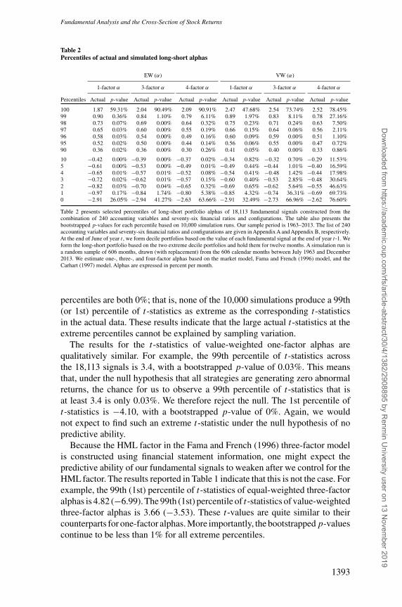
Table 2Percentiles of actual and simulated long-short alphas
EW (α) VW (α)
1-factor α 3-factor α 4-factor α 1-factor α 3-factor α 4-factor α
Percentiles Actual p-value Actual p-value Actual p-value Actual p-value Actual p-value Actual p-value
100 1.87 59.31% 2.04 90.49% 2.09 90.91% 2.47 47.68% 2.54 73.74% 2.52 78.45%99 0.90 0.36% 0.84 1.10% 0.79 6.11% 0.89 1.97% 0.83 8.11% 0.78 27.16%98 0.73 0.07% 0.69 0.00% 0.64 0.32% 0.75 0.23% 0.71 0.24% 0.63 7.50%97 0.65 0.03% 0.60 0.00% 0.55 0.19% 0.66 0.15% 0.64 0.06% 0.56 2.11%96 0.58 0.03% 0.54 0.00% 0.49 0.16% 0.60 0.09% 0.59 0.00% 0.51 1.10%95 0.52 0.02% 0.50 0.00% 0.44 0.14% 0.56 0.06% 0.55 0.00% 0.47 0.72%90 0.36 0.02% 0.36 0.00% 0.30 0.26% 0.41 0.05% 0.40 0.00% 0.33 0.86%
10 −0.42 0.00% −0.39 0.00% −0.37 0.02% −0.34 0.82% −0.32 0.70% −0.29 11.53%5 −0.61 0.00% −0.53 0.00% −0.49 0.01% −0.49 0.44% −0.44 1.01% −0.40 16.59%4 −0.65 0.01% −0.57 0.01% −0.52 0.08% −0.54 0.41% −0.48 1.42% −0.44 17.98%3 −0.72 0.02% −0.62 0.01% −0.57 0.15% −0.60 0.40% −0.53 2.85% −0.48 30.64%2 −0.82 0.03% −0.70 0.04% −0.65 0.32% −0.69 0.65% −0.62 5.64% −0.55 46.63%1 −0.97 0.17% −0.84 1.74% −0.80 5.38% −0.85 4.32% −0.74 36.31% −0.69 69.73%0 −2.91 26.05% −2.94 41.27% −2.63 63.66% −2.91 32.49% −2.73 66.96% −2.62 76.60%
Table 2 presents selected percentiles of long-short portfolio alphas of 18,113 fundamental signals constructed from thecombination of 240 accounting variables and seventy-six financial ratios and configurations. The table also presents thebootstrapped p-values for each percentile based on 10,000 simulation runs. Our sample period is 1963–2013. The list of 240accounting variables and seventy-six financial ratios and configurations are given in Appendix A and Appendix B, respectively.At the end of June of year t , we form decile portfolios based on the value of each fundamental signal at the end of year t-1. Weform the long-short portfolio based on the two extreme decile portfolios and hold them for twelve months. A simulation run isa random sample of 606 months, drawn (with replacement) from the 606 calendar months between July 1963 and December2013. We estimate one-, three-, and four-factor alphas based on the market model, Fama and French (1996) model, and theCarhart (1997) model. Alphas are expressed in percent per month.
percentiles are both 0%; that is, none of the 10,000 simulations produce a 99th(or 1st) percentile of t-statistics as extreme as the corresponding t-statisticsin the actual data. These results indicate that the large actual t-statistics at theextreme percentiles cannot be explained by sampling variation.
The results for the t-statistics of value-weighted one-factor alphas arequalitatively similar. For example, the 99th percentile of t-statistics acrossthe 18,113 signals is 3.4, with a bootstrapped p-value of 0.03%. This meansthat, under the null hypothesis that all strategies are generating zero abnormalreturns, the chance for us to observe a 99th percentile of t-statistics that isat least 3.4 is only 0.03%. We therefore reject the null. The 1st percentile oft-statistics is −4.10, with a bootstrapped p-value of 0%. Again, we wouldnot expect to find such an extreme t-statistic under the null hypothesis of nopredictive ability.
Because the HML factor in the Fama and French (1996) three-factor modelis constructed using financial statement information, one might expect thepredictive ability of our fundamental signals to weaken after we control for theHML factor. The results reported in Table 1 indicate that this is not the case. Forexample, the 99th (1st) percentile of t-statistics of equal-weighted three-factoralphas is 4.82 (−6.99). The 99th (1st) percentile of t-statistics of value-weightedthree-factor alphas is 3.66 (−3.53). These t-values are quite similar to theircounterparts for one-factor alphas. More importantly, the bootstrappedp-valuescontinue to be less than 1% for all extreme percentiles.
1393
Dow
nloaded from https://academ
ic.oup.com/rfs/article-abstract/30/4/1382/2908895 by R
enmin U
niversity user on 13 Novem
ber 2019
The Review of Financial Studies / v 30 n 4 2017
We note that the magnitudes of the four-factor alpha t-statistics are slightlylower than those of one- and three-factor alphas. For example, the 99th (1st)percentile of equal-weighted four-factor alpha t-statistics is 4.35 (−6.13),compared to 4.82 (−6.99) for three-factor alpha t-statistics. Nevertheless,the bootstrapped p-values for the extreme percentiles of four-factor alphat-statistics are all less than 1% for equal-weighted portfolios and less than5% for value-weighted portfolios, so our inferences are unchanged. Overall,the evidence in Table 1 strongly indicates that the superior performance oftop-ranked signals cannot be attributed to random chance.
2.1.2 Bootstrap alphas. In Table 2, we apply the bootstrap procedure toalphas. Although t-statistics have better sampling properties and are less proneto the outlier problem, alphas better measure the economic magnitude of theabnormal performance. Therefore, the results for alphas will be of significantinterest to practitioners and investors. The format of Table 2 is identical to thatof Table 1 except that the numbers reported in column “Actual” are alphasrather than t-statistics.
The equal-weighted results show that the extreme percentiles of alphas areeconomically large and not attributable to sampling variation. For example, the99th percentile of equal-weighted one-factor alphas is 0.9% per month and isgreater than its counterpart in all but 0.36% of the simulation runs. Similarly, the1st percentile of equal-weighted one-factor alphas is −0.97% per month, witha bootstrapped p-value of 0.17%. The maximum and minimum alphas, that is,the 100th percentile and the 0th percentile are generally insignificant in partbecause of the outlier problem associated with alpha estimates.10 The resultsfor three-factor and four-factor alphas are qualitatively similar. All extremepercentiles except the minimum and the maximum are significant.
The right panel of Table 2 presents the value-weighted results. The one-and three-factor alpha results are generally significant. For example, the 99thpercentile of one-factor alphas is 0.89% per month, with a bootstrapped p-valueof 1.97%. The 99th percentile of three-factor alphas is 0.83% per month, witha bootstrapped p-value of 8.11%. The four-factor alpha results are somewhatweaker. For example, the 99th percentile of four-factor alphas is 0.78% permonth, with a bootstrapped p-value of 27.16%. However, for the 90th through98th percentiles, we find the bootstrapped value to be less than 10%, and in mostcases less than 5%. Overall, despite the relatively poor sampling properties ofalpha estimates, we find evidence that the extreme alphas of the best performingsignals are not due to sampling variation.
10 If a fundamental signal has a short sample period or exhibits high residual variance, its alpha estimates will tendto be spurious outliers in the cross-section (Kosowski et al. 2006). This outlier problem is more severe in thesimulated samples. As a result, the bootstrapped p-values for the most extreme percentiles of alphas tend to belarge.
1394
Dow
nloaded from https://academ
ic.oup.com/rfs/article-abstract/30/4/1382/2908895 by R
enmin U
niversity user on 13 Novem
ber 2019
Fundamental Analysis and the Cross-Section of Stock Returns
2.2 Performance persistenceWe next examine the stability and persistence of the long-short performanceof fundamental signals over time. This analysis is important because previousstudies (e.g., Sullivan, Timmermann, and White 2001) argue that the analysisof subperiod stability is a remedy against data mining.
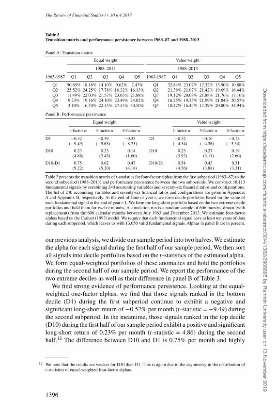
2.2.1 Transition matrix. To measure stability, we divide our sample periodinto two halves of roughly equal length (1963–87 and 1988–2013) and thenconstruct a transition matrix for the t-statistics between the two subperiods.Specifically, we sort signals into quintiles (Q1 through Q5) based on their four-factor alpha t-statistics during each subperiod and report the percentage ofsignals in a given quintile during the first half of the sample period moving toa particular quintile in the second half. If the predictive ability of fundamentalsignals is due to chance, then we should expect all numbers in the transitionmatrix to be around 20% (the unconditional average). On the other hand, ifthe predictive ability is real and stable, then we should expect the probabilitiesof Q1 → Q1 and Q5 → Q5 to be significantly greater than 20%, and theprobabilities of Q1 → Q5 and Q5 → Q1 to be significantly less than 20%.
Panel A of Table 3 reports the results. Focusing on equal-weighted returnsin the left panel, we find strong evidence of cross-period stability. More than50% of the signals ranked in Q1 (signals with the largest negative t-statistics)during the first half of the sample period continue to be ranked in Q1 during thesecond half, while less than 8% of these signals move to Q5 (signals with thelargest positive t-statistics). Similarly, more than 30% of the signals ranked inQ5 continue to stay in Q5 during the second half of the sample period, whileonly 3.1% of the signals switch to Q1.11 Unreported tests indicate that thesepercentages are significantly different from 20%.
The results for value-weighted returns are reported in the right panel. Wefind that about 33% of the signals ranked in the bottom quintile during thefirst subperiod continue to be ranked in the bottom quintile during the secondsubperiod, while less than 11% of these signals move to the top quintile.Similarly, nearly 35% of the signals ranked in the top quintile continue tostay in the same quintile during the second half of the sample period, whileabout 11% of the signals switch to the bottom quintile. More importantly, thesepercentages are statistically different from 20%.
2.2.2 Performance persistence. Another way to evaluate whether thepredictive ability of fundamental signals is stable is to look at the performancepersistence of fundamental-based trading strategies. This is a common approachin the mutual fund and hedge fund literature to separate skill from luck. As in
11 We note that the persistence is stronger for Q5 than for Q1. This is due to the asymmetry in the distributionof t-statistics of equal-weighted four-factor alphas. Table 1 reports that the 90th percentile of equal-weightedfour-factor alpha t-statistic is 2.12, whereas the 10th percentile is −3.17.
1395
Dow
nloaded from https://academ
ic.oup.com/rfs/article-abstract/30/4/1382/2908895 by R
enmin U
niversity user on 13 Novem
ber 2019
The Review of Financial Studies / v 30 n 4 2017
Table 3Transition matrix and performance persistence between 1963–87 and 1988–2013
Panel A: Transition matrix
Equal weight Value weight
1988–2013 1988–2013
1963-1987 Q1 Q2 Q3 Q4 Q5 1963-1987 Q1 Q2 Q3 Q4 Q5
Q1 50.65% 18.16% 14.10% 9.62% 7.47% Q1 32.84% 23.07% 17.32% 15.90% 10.88%Q2 25.52% 24.25% 17.78% 16.32% 16.13% Q2 21.38% 21.07% 21.42% 19.69% 16.44%Q3 11.49% 22.03% 21.57% 23.03% 21.88% Q3 19.12% 20.08% 21.88% 21.76% 17.16%Q4 9.23% 19.16% 24.10% 23.49% 24.02% Q4 16.25% 19.35% 21.99% 21.84% 20.57%Q5 3.10% 16.40% 22.45% 27.55% 30.50% Q5 10.42% 16.44% 17.39% 20.80% 34.94%
Panel B: Performance persistence
Equal weight Value weight
1-factor α 3-factor α 4-factor α 1-factor α 3-factor α 4-factor α
D1 −0.52 −0.39 −0.33 D1 −0.32 −0.16 −0.12(−9.49) (−9.63) (−8.75) (−4.54) (−4.36) (−3.54)
D10 0.23 0.23 0.14 D10 0.23 0.27 0.19(4.86) (2.43) (1.60) (3.92) (3.11) (2.60)
D10-D1 0.75 0.62 0.47 D10-D1 0.54 0.43 0.31(9.22) (5.20) (4.18) (4.56) (3.88) (3.31)
Table 3 presents the transition matrix of t-statistics for four-factor alphas from the first subperiod (1963–87) to thesecond subperiod (1988–2013) and performance persistence between the two subperiods. We construct 18,113fundamental signals by combining 240 accounting variables and seventy-six financial ratios and configurations.The list of 240 accounting variables and seventy-six financial ratios and configurations are given in AppendixA and Appendix B, respectively. At the end of June of year t , we form decile portfolios based on the value ofeach fundamental signal at the end of year t-1. We form the long-short portfolio based on the two extreme decileportfolios and hold them for twelve months. A simulation run is a random sample of 606 months, drawn (withreplacement) from the 606 calendar months between July 1963 and December 2013. We estimate four-factoralphas based on the Carhart (1997) model. We require that each fundamental signal have at least ten years of dataduring each subperiod, which leaves us with 13,050 valid fundamental signals. Alphas in panel B are in percent.
our previous analysis, we divide our sample period into two halves. We estimatethe alpha for each signal during the first half of our sample period. We then sortall signals into decile portfolios based on the t-statistics of the estimated alpha.We form equal-weighted portfolios of these anomalies and hold the portfoliosduring the second half of our sample period. We report the performance of thetwo extreme deciles as well as their difference in panel B of Table 3.
We find strong evidence of performance persistence. Looking at the equal-weighted one-factor alphas, we find that those signals ranked in the bottomdecile (D1) during the first subperiod continue to exhibit a negative andsignificant long-short return of −0.52% per month (t-statistic = −9.49) duringthe second subperiod. In the meantime, those signals ranked in the top decile(D10) during the first half of our sample period exhibit a positive and significantlong-short return of 0.23% per month (t-statistic = 4.86) during the secondhalf.12 The difference between D10 and D1 is 0.75% per month and highly
12 We note that the results are weaker for D10 than D1. This is again due to the asymmetry in the distribution oft-statistics of equal-weighted four-factor alphas.
1396
Dow
nloaded from https://academ
ic.oup.com/rfs/article-abstract/30/4/1382/2908895 by R
enmin U
niversity user on 13 Novem
ber 2019
Fundamental Analysis and the Cross-Section of Stock Returns
statistically significant. The result is robust whether we use three- or four-factoralphas and whether we examine equal-weighted or value-weighted long-shortreturns. The difference between D10 and D1 is economically meaningful andstatistically significant across all specifications.
Overall, our analysis of the performance persistence of fundamental-basedsignals across subperiods provides further evidence that the predictive abilityof fundamental signals is unlikely to be driven by random chance. It alsosuggests that investors could have adopted a recursive decision rule to identifythe best performing signals and have used this information to produce genuinelysuperior out-of-sample performance.
2.3 Evidence on mispricing- and risk-based explanationsHaving shown that the superior performance of top-ranked fundamental signalsis not due to random chance, we next investigate whether it is consistent withmispricing- or risk-based explanations.
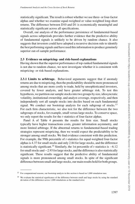
2.3.1 Limits to arbitrage. Behavioral arguments suggest that if anomalyreturns are due to mispricing, then the predictability should be more pronouncedamong stocks that are more costly to trade, held by unsophisticated investors,covered by fewer analysts, and have greater arbitrage risk. To test thishypothesis, we partition our sample stocks into two groups by size, idiosyncraticvolatility, institutional ownership, and analyst coverage, respectively, and thenindependently sort all sample stocks into deciles based on each fundamentalsignal. We conduct our bootstrap analysis for each subgroup of stocks.13
For each firm characteristic, we also test for the difference between the twosubgroups of stocks, for example, small versus large stocks. To conserve space,we only report the results for the t-statistics of four-factor alphas.
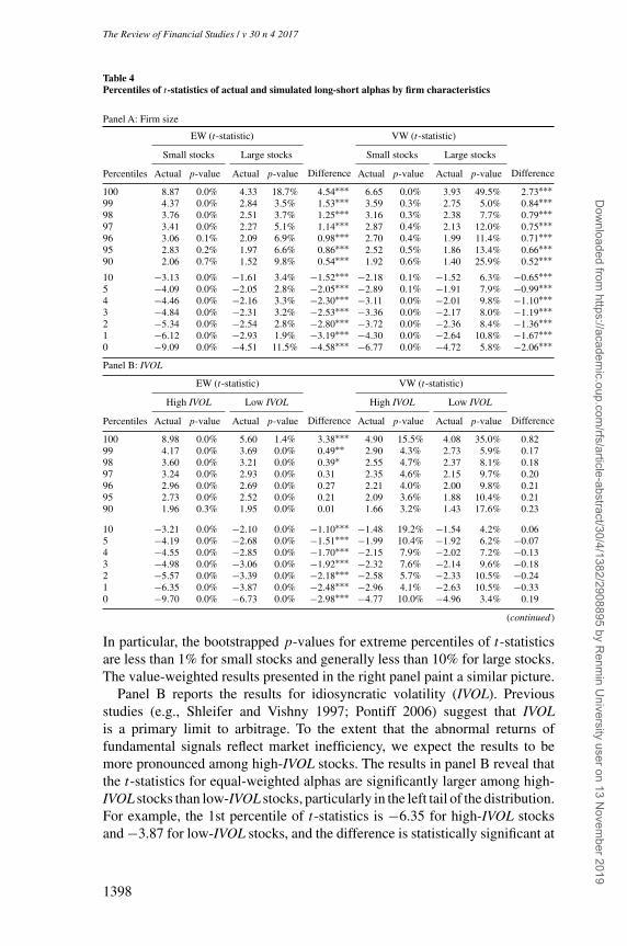
Panel A of Table 4 presents the results for firm size. Small stockstypically have higher transactions costs, greater information asymmetry, andmore limited arbitrage. If the abnormal returns to fundamental-based tradingstrategies represent mispricing, then we would expect the predictability to bestronger among small stocks. We find evidence consistent with this prediction.For example, the 99th percentile of t-statistics for equal-weighted four-factoralphas is 4.37 for small stocks and only 2.84 for large stocks, and the differenceis statistically significant.14 Similarly, the 1st percentile of t-statistics is −6.12for small stocks and−2.93 for large stocks, and the difference is also statisticallysignificant. These results suggest that the predictive ability of fundamentalsignals is more pronounced among small stocks. In spite of the significantdifference between small and large stocks, our main results hold for both groups.
13 For computational reasons, our bootstrap analysis in this section is based on 1,000 simulation runs.
14 We evaluate the statistical significance of the difference between small and large stocks by using the standarddeviation of this difference across 1,000 simulations as the standard error.
1397
Dow
nloaded from https://academ
ic.oup.com/rfs/article-abstract/30/4/1382/2908895 by R
enmin U
niversity user on 13 Novem
ber 2019
The Review of Financial Studies / v 30 n 4 2017
Table 4Percentiles of t-statistics of actual and simulated long-short alphas by firm characteristics
Panel A: Firm size
EW (t-statistic) VW (t-statistic)
Small stocks Large stocks
Difference
Small stocks Large stocks
DifferencePercentiles Actual p-value Actual p-value Actual p-value Actual p-value
100 8.87 0.0% 4.33 18.7% 4.54∗∗∗ 6.65 0.0% 3.93 49.5% 2.73∗∗∗99 4.37 0.0% 2.84 3.5% 1.53∗∗∗ 3.59 0.3% 2.75 5.0% 0.84∗∗∗98 3.76 0.0% 2.51 3.7% 1.25∗∗∗ 3.16 0.3% 2.38 7.7% 0.79∗∗∗97 3.41 0.0% 2.27 5.1% 1.14∗∗∗ 2.87 0.4% 2.13 12.0% 0.75∗∗∗96 3.06 0.1% 2.09 6.9% 0.98∗∗∗ 2.70 0.4% 1.99 11.4% 0.71∗∗∗95 2.83 0.2% 1.97 6.6% 0.86∗∗∗ 2.52 0.5% 1.86 13.4% 0.66∗∗∗90 2.06 0.7% 1.52 9.8% 0.54∗∗∗ 1.92 0.6% 1.40 25.9% 0.52∗∗∗10 −3.13 0.0% −1.61 3.4% −1.52∗∗∗ −2.18 0.1% −1.52 6.3% −0.65∗∗∗5 −4.09 0.0% −2.05 2.8% −2.05∗∗∗ −2.89 0.1% −1.91 7.9% −0.99∗∗∗4 −4.46 0.0% −2.16 3.3% −2.30∗∗∗ −3.11 0.0% −2.01 9.8% −1.10∗∗∗3 −4.84 0.0% −2.31 3.2% −2.53∗∗∗ −3.36 0.0% −2.17 8.0% −1.19∗∗∗2 −5.34 0.0% −2.54 2.8% −2.80∗∗∗ −3.72 0.0% −2.36 8.4% −1.36∗∗∗1 −6.12 0.0% −2.93 1.9% −3.19∗∗∗ −4.30 0.0% −2.64 10.8% −1.67∗∗∗0 −9.09 0.0% −4.51 11.5% −4.58∗∗∗ −6.77 0.0% −4.72 5.8% −2.06∗∗∗
Panel B: IVOL
EW (t-statistic) VW (t-statistic)
High IVOL Low IVOL
Difference
High IVOL Low IVOL
DifferencePercentiles Actual p-value Actual p-value Actual p-value Actual p-value
100 8.98 0.0% 5.60 1.4% 3.38∗∗∗ 4.90 15.5% 4.08 35.0% 0.8299 4.17 0.0% 3.69 0.0% 0.49∗∗ 2.90 4.3% 2.73 5.9% 0.1798 3.60 0.0% 3.21 0.0% 0.39∗ 2.55 4.7% 2.37 8.1% 0.1897 3.24 0.0% 2.93 0.0% 0.31 2.35 4.6% 2.15 9.7% 0.2096 2.96 0.0% 2.69 0.0% 0.27 2.21 4.0% 2.00 9.8% 0.2195 2.73 0.0% 2.52 0.0% 0.21 2.09 3.6% 1.88 10.4% 0.2190 1.96 0.3% 1.95 0.0% 0.01 1.66 3.2% 1.43 17.6% 0.23
10 −3.21 0.0% −2.10 0.0% −1.10∗∗∗ −1.48 19.2% −1.54 4.2% 0.065 −4.19 0.0% −2.68 0.0% −1.51∗∗∗ −1.99 10.4% −1.92 6.2% −0.074 −4.55 0.0% −2.85 0.0% −1.70∗∗∗ −2.15 7.9% −2.02 7.2% −0.133 −4.98 0.0% −3.06 0.0% −1.92∗∗∗ −2.32 7.6% −2.14 9.6% −0.182 −5.57 0.0% −3.39 0.0% −2.18∗∗∗ −2.58 5.7% −2.33 10.5% −0.241 −6.35 0.0% −3.87 0.0% −2.48∗∗∗ −2.96 4.1% −2.63 10.5% −0.330 −9.70 0.0% −6.73 0.0% −2.98∗∗∗ −4.77 10.0% −4.96 3.4% 0.19
(continued )
In particular, the bootstrapped p-values for extreme percentiles of t-statisticsare less than 1% for small stocks and generally less than 10% for large stocks.The value-weighted results presented in the right panel paint a similar picture.
Panel B reports the results for idiosyncratic volatility (IVOL). Previousstudies (e.g., Shleifer and Vishny 1997; Pontiff 2006) suggest that IVOLis a primary limit to arbitrage. To the extent that the abnormal returns offundamental signals reflect market inefficiency, we expect the results to bemore pronounced among high-IVOL stocks. The results in panel B reveal thatthe t-statistics for equal-weighted alphas are significantly larger among high-IVOL stocks than low-IVOL stocks, particularly in the left tail of the distribution.For example, the 1st percentile of t-statistics is −6.35 for high-IVOL stocksand −3.87 for low-IVOL stocks, and the difference is statistically significant at
1398
Dow
nloaded from https://academ
ic.oup.com/rfs/article-abstract/30/4/1382/2908895 by R
enmin U
niversity user on 13 Novem
ber 2019
Fundamental Analysis and the Cross-Section of Stock Returns
Table 4Continued
Panel C: IO
EW (t-statistic) VW (t-statistic)
Low IO High IO
Difference
Low IO High IO
DifferencePercentiles Actual p-value Actual p-value Actual p-value Actual p-value
100 8.74 0.0% 4.94 7.7% 3.80∗∗∗ 5.03 7.0% 3.62 79.1% 1.41∗99 4.15 0.0% 3.31 0.7% 0.83∗∗∗ 3.11 1.0% 2.55 25.1% 0.56∗∗∗98 3.55 0.0% 2.89 1.3% 0.66∗∗∗ 2.67 2.1% 2.27 22.7% 0.40∗∗∗97 3.17 0.1% 2.65 1.2% 0.53∗∗∗ 2.39 4.3% 2.04 28.7% 0.35∗96 2.93 0.1% 2.46 1.4% 0.46∗∗∗ 2.23 4.2% 1.89 30.2% 0.35∗∗95 2.70 0.3% 2.33 1.2% 0.38∗∗ 2.08 5.1% 1.77 31.6% 0.32∗90 2.00 0.5% 1.79 2.2% 0.21 1.60 7.2% 1.37 35.3% 0.23
10 −3.07 0.0% −2.08 0.0% −0.99∗∗∗ −1.54 10.6% −1.50 13.0% −0.045 −4.09 0.0% −2.67 0.0% −1.41∗∗∗ −2.01 7.6% −1.91 12.7% −0.114 −4.39 0.0% −2.86 0.0% −1.53∗∗∗ −2.16 6.6% −2.02 12.8% −0.133 −4.81 0.0% −3.08 0.0% −1.73∗∗∗ −2.34 5.4% −2.17 12.6% −0.172 −5.32 0.0% −3.31 0.0% −2.00∗∗∗ −2.58 4.1% −2.37 12.1% −0.211 −5.95 0.0% −3.65 0.1% −2.30∗∗∗ −2.94 3.6% −2.73 9.4% −0.220 −10.05 0.0% −5.49 2.6% −4.56∗∗∗ −5.19 2.1% −4.46 15.1% −0.73
Panel D: Analyst coverage
EW (t-statistic) VW (t-statistic)
Low coverage High coverage
Difference
Low coverage High coverage
DifferencePercentiles Actual p-value Actual p-value Actual p-value Actual p-value
100 9.96 0.0% 5.20 4.3% 4.76∗∗∗ 5.84 0.9% 4.03 46.9% 1.80∗∗∗99 4.51 0.0% 3.30 0.7% 1.21∗∗∗ 3.49 0.0% 2.75 5.6% 0.74∗∗∗98 3.76 0.0% 2.92 0.7% 0.84∗∗∗ 3.05 0.0% 2.43 6.7% 0.62∗∗∗97 3.32 0.0% 2.69 0.7% 0.63∗∗∗ 2.70 0.0% 2.20 9.7% 0.50∗∗∗96 3.02 0.1% 2.50 0.9% 0.52∗∗∗ 2.50 0.0% 2.04 11.6% 0.46∗∗∗95 2.80 0.0% 2.35 1.0% 0.45∗∗∗ 2.35 0.0% 1.91 12.4% 0.44∗∗∗90 2.15 0.0% 1.83 1.7% 0.32∗ 1.75 0.6% 1.44 21.3% 0.31∗∗∗10 −3.32 0.0% −2.07 0.2% −1.25∗∗∗ −1.82 0.7% −1.51 12.0% −0.31∗∗5 −4.36 0.0% −2.66 0.1% −1.71∗∗∗ −2.37 0.1% −1.95 10.0% −0.43∗∗∗4 −4.67 0.0% −2.81 0.1% −1.85∗∗∗ −2.57 0.1% −2.08 9.0% −0.49∗∗∗3 −5.07 0.0% −3.00 0.1% −2.08∗∗∗ −2.79 0.1% −2.23 9.1% −0.56∗∗∗2 −5.68 0.0% −3.25 0.1% −2.43∗∗∗ −3.04 0.1% −2.44 7.7% −0.60∗∗∗1 −6.62 0.0% −3.71 0.1% −2.91∗∗∗ −3.47 0.0% −2.74 8.4% −0.73∗∗∗0 −9.22 0.4% −6.40 0.1% −2.82∗∗∗ −5.40 2.0% −4.38 20.8% −1.02
Table 4 presents selected percentiles of the t-statistics for long-short portfolio alphas of 18,113 fundamentalsignals constructed from the combination of 240 accounting variables and seventy-six financial ratios andconfigurations. The table also presents the bootstrapped p-values for each percentile based on 1,000 simulationruns. Our sample period is 1963–2013. The list of 240 accounting variables and seventy-six financial ratios andconfigurations are given in Appendix A and Appendix B, respectively. At the end of June of year t , we formdecile portfolios based on the value of each fundamental signal at the end of year t-1. We also independentlysort all sample firms into two groups based on firm size, B/M, idiosyncratic volatility, institutional ownership,and analyst coverage, respectively. For each subsample of firms by characteristics, we compute long-short hedgereturns and the associated alphas based on the two extreme decile portfolios. A simulation run is a random sampleof 606 months, drawn (with replacement) from the 606 calendar months between July 1963 and December 2013.To ensure a sufficiently large sample, we require a minimum of five years of observation for a signal to beincluded in the analysis. We estimate four-factor alphas based on the Carhart (1997) model. Superscripts ∗∗∗,∗∗, and ∗ indicate statistical significance at 1%, 5%, and 10% levels, respectively.
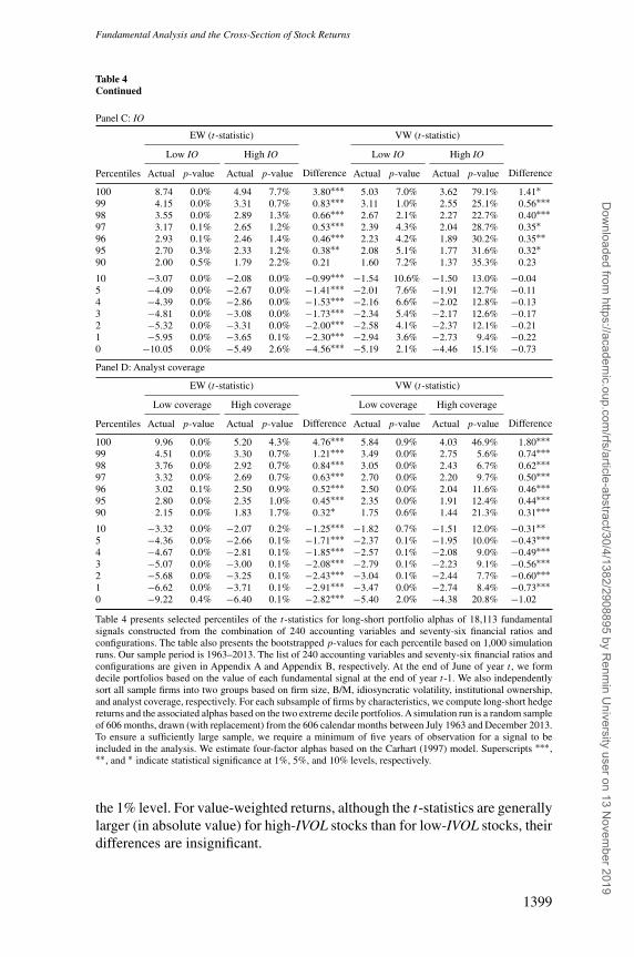
the 1% level. For value-weighted returns, although the t-statistics are generallylarger (in absolute value) for high-IVOL stocks than for low-IVOL stocks, theirdifferences are insignificant.
1399
Dow
nloaded from https://academ
ic.oup.com/rfs/article-abstract/30/4/1382/2908895 by R
enmin U
niversity user on 13 Novem
ber 2019
The Review of Financial Studies / v 30 n 4 2017
Panel C presents the results for institutional ownership (IO).15 Institutionalinvestors are more sophisticated than individual investors. To the extent thatthe predictive ability of fundamental signals represent misreaction to publicaccounting information by unsophisticated investors, we would expect thispredictability to be stronger among low-institutional ownership stocks. Ourresults confirm this conjecture. For equal-weighed returns, we find large andstatistically significant differences in t-statistics between high- and low-IOstocks. For example, the 99th percentile of t-statistics is 4.15 for low-IOstocks and 3.31 for high-IO stocks, with the difference being statisticallysignificant at the 1% level. The value-weighted results continue to suggestthat the predictability is stronger among low-IO stocks than high-IO stocks.
In panel D, we focus on analyst coverage.16 Financial analysts play animportant role in interpreting and disseminating financial information. If thepredictive ability of fundamental signals is due to the market’s failing tofully incorporate public financial statement information, we would expectthis predictability to be attenuated among stocks with more extensive analystcoverage. The results contained in panel D of Table 4 lend strong support tothis prediction. We find statistically significant difference in t-statistics betweenlow- and high-analyst coverage stocks, whether we examine equal-weightedor value-weighted returns. Overall, consistent with behavioral explanations,we find that the predictive ability of fundamental signals is more pronouncedamong small stocks and stocks with higher idiosyncratic volatility, lowerinstitutional ownership, and fewer analysts.17
2.3.2 Investor sentiment. To the extent that mispricing exists, overpricingshould be more prevalent than underpricing because shorting is more costly. Assuch, anomaly returns should be significantly higher following high-sentimentperiods than low-sentiment periods (Stambaugh, Yu, and Yuan 2012). We testthis prediction for our sample of fundamental signals. We obtain the investorsentiment index of Baker and Wurgler (2006) from Jeffrey Wurgler’s website.18
Following Stambaugh, Yu, and Yuan (2012), we divide our sample into high-and low-sentiment periods based on the median sentiment index level over oursample period. We then compute anomaly returns separately for the periodsfollowing high- and low-sentiment levels. We perform this analysis for the top10%, 5%, and 1% of fundamental signals (ranked based on the absolute valueof the t-statistics of four-factor alphas).
15 We obtain institutional ownership data from the Thomson Reuters 13F database. Due to data availability, thesample period for this analysis is from 1979 to 2013.
16 We obtain the analyst coverage data from IBES. The sample period for this analysis is from 1976 to 2013.
17 We also conduct a bootstrap analysis on alphas. We find qualitatively similar results to those in Table 4. Toconserve space, we report the results of this analysis in Table IA.4 of the Internet Appendix.
18 We thank Jeffery Wurgler for making this data available on his website, http://people.stern.nyu.edu/jwurgler/.
1400
Dow
nloaded from https://academ
ic.oup.com/rfs/article-abstract/30/4/1382/2908895 by R
enmin U
niversity user on 13 Novem
ber 2019
Fundamental Analysis and the Cross-Section of Stock Returns
Table 5Investor sentiment, business cycle, and anomaly returns
Panel A: Investor sentiment
EW (α) VW (α)
Signals High sentiment Low sentiment Difference Signals High sentiment Low sentiment Difference
Top 10% 0.56 0.36 0.20 Top 10% 0.62 0.29 0.33(11.25) (9.02) (3.15) (10.61) (6.40) (4.47)
Top 5% 0.63 0.41 0.22 Top 5% 0.70 0.31 0.39(10.82) (8.67) (2.97) (10.38) (5.73) (4.55)
Top 1% 0.76 0.49 0.26 Top 1% 0.88 0.35 0.53(10.53) (8.57) (2.84) (10.45) (4.91) (4.83)
Panel B: Business cycle
EW (α) VW (α)
Signals Recession Expansion Difference Signals Recession Expansion Difference
Top 10% 0.48 0.44 0.04 Top 10% 0.57 0.41 0.17(5.42) (14.09) (0.46) (4.58) (11.83) (1.30)
Top 5% 0.55 0.50 0.05 Top 5% 0.67 0.45 0.22(5.14) (13.69) (0.48) (4.45) (11.16) (1.43)
Top 1% 0.72 0.59 0.13 Top 1% 0.73 0.55 0.19(5.19) (12.97) (0.89) (3.99) (11.00) (0.97)
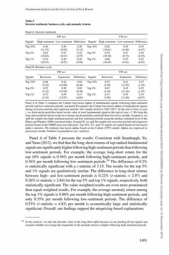
Panel A of Table 5 compares the Carhart four-factor alphas of fundamental signals following high-sentimentperiods and low-sentiment periods, and panel B compares the Carhart four-factor alphas of fundamental signalsduring recession periods and expansion periods. Our sample period is 1963–2013. At the end of June of yeart , we form decile portfolios based on the value of each fundamental signal at the end of year t-1. We form thelong-short portfolio based on the two extreme decile portfolios and hold them for twelve months. In panel A, wesplit the sample into high-sentiment periods and low-sentiment periods using the median sentiment level of theBaker and Wurgler (2006) sentiment index. In panel B, we split the sample into recession periods and expansionperiods based on the NBER recession indicators. Top 10%, 5%, and 1% signals are ranked based on four-factoralpha t-statistics. We estimate four-factor alphas based on the Carhart (1997) model. Alphas are expressed inpercent per month. Numbers in parentheses are t-statistics.
Panel A of Table 5 presents the results. Consistent with Stambaugh, Yu,and Yuan (2012), we find that the long-short returns of top-ranked fundamentalsignals are significantly higher following high-sentiment periods than followinglow-sentiment periods. For example, the average long-short return for thetop 10% signals is 0.56% per month following high-sentiment periods, and0.36% per month following low-sentiment periods.19 The difference of 0.2%is statistically significant with a t-statistic of 3.15. The results for the top 5%and 1% signals are qualitatively similar. The difference in long-short returnsbetween high- and low-sentiment periods is 0.22% (t-statistic = 2.97) and0.26% (t-statistic = 2.84) for the top 5% and top 1% signals, respectively, bothstatistically significant. The value-weighted results are even more pronouncedthan equal-weighted results. For example, the average anomaly return amongthe top 1% signals is 0.88% per month following high-sentiment periods, andonly 0.35% per month following low-sentiment periods. The difference of0.53% (t-statistic = 4.83) per month is economically large and statisticallysignificant. Overall, our findings support the mispricing-based explanations.
19 In this analysis, we take the absolute value of the long-short alpha because we are pooling all top signals andexamine whether on average the magnitude of the anomaly returns is higher following high-sentiment periods.
1401
Dow
nloaded from https://academ
ic.oup.com/rfs/article-abstract/30/4/1382/2908895 by R
enmin U
niversity user on 13 Novem
ber 2019
The Review of Financial Studies / v 30 n 4 2017
2.3.3 Business cycle. In this section, we examine whether anomaly returnsvary across the business cycle (Chordia and Shivakumar 2002). If the superiorperformance of top fundamental signals represents compensation for systematicrisk, then we should expect the long-short returns to be significantly lowerduring bad times (e.g., recessions) than during good times (e.g., expansions).Cochrane (2004, 3) explains the basic intuition of this test:
Other things equal, an asset that does badly in states of nature like arecession, in which the investor feels poor and is consuming little,is less desirable than an asset does badly in states of nature likea boom in which the investor feels wealthy and is consuming agreat deal. The former asset will sell for a lower price; its price willreflect a discount for its riskiness.
We obtain NBER recession dates from the Federal Reserve Bank of St. Louis’website.20 Similar to our investor sentiment analysis, we focus on the top 10%,top 5%, and top 1% fundamental signals ranked based on the t-statistics offour-factor alphas. Panel B of Table 5 presents the results for this analysis.Contrary to the prediction of risk-based explanations, we find that the long-short returns of top fundamental signals are actually higher during recessionperiods than during expansion periods, although the difference is statisticallyinsignificant. For example, the average equal-weighted four-factor alpha for thetop 1% signals is 0.72% per month during recessions and is 0.59% per monthduring expansions, both of which are highly statistically significant. Similarly,the average value-weighted four-factor alpha is 0.73% during recessions and0.55% during expansions. Overall, our evidence is inconsistent with the ideathat fundamental anomalies are driven by exposure to macroeconomic risksrelated to the business cycle.
In summary, we have presented evidence that the predictive ability offundamental signals varies predictably across subgroups of stocks sortedby proxies for limits to arbitrage. We have also shown that fundamentalanomalies are more pronounced following high-sentiment periods. In addition,the anomaly returns are unrelated to the business cycle. Although we cannotrule out risk-based explanations, our results suggest that fundamental-basedanomalies are more consistent with mispricing-based explanations.
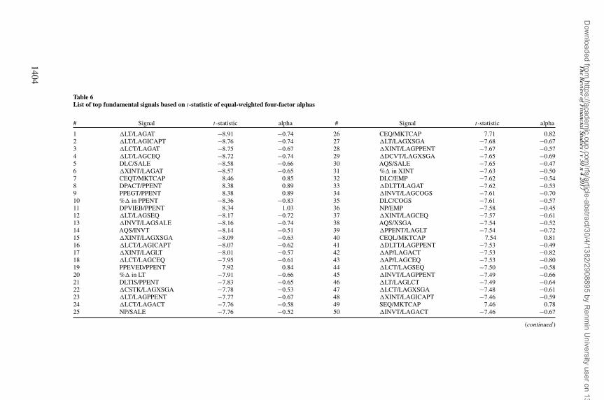
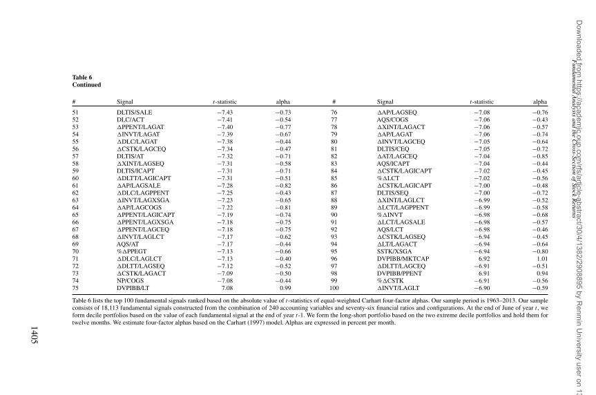
2.4 Top fundamental anomalies2.4.1 What are the top signals?. Our bootstrap results indicate that a largenumber of fundamental signals exhibit genuine predictive ability for futurestock returns. In Table 6, we report the top 100 fundamental signals ranked based
20 https://research.stlouisfed.org/fred2/.
1402
Dow
nloaded from https://academ
ic.oup.com/rfs/article-abstract/30/4/1382/2908895 by R
enmin U
niversity user on 13 Novem
ber 2019
Fundamental Analysis and the Cross-Section of Stock Returns
on the absolute value of the t-statistics of equal-weighted four-factor alphas.For each fundamental signal on this list, we also report its corresponding alphaand t-statistic. For example, the top-ranked signal is �LT/LAGAT (change intotal liabilities divided by lagged total assets), with a monthly alpha of −0.74%and a t-statistic of −8.91.
Broadly speaking, the top signals reported in Table 6 can be classified intothree groups. The first group contains those that have been documented in theprior literature, for example, the book-to-market ratio (CEQ/MKTCAP andSEQ/MKTCAP) and inventory change (�INVT/LAGAT). The second groupcontains fundamental signals that are closely related to those that have beendocumented in the literature, for example, �LT/LAGAT (total liability change)and %� in LT (growth in total liability). Both of these signals are closelyrelated to the asset growth measure of Cooper, Gulen, and Schill (2008). Alarge number of the fundamental signals on this list, however, belong to the thirdgroup, which have not been directly examined by prior studies, for example,�XINT/LAGAT (change in interest expense divided by lagged total assets),DPACT/PPENT (accumulated depreciation divided by total net property, plant,and equipment), and DLC/EMP (short-term debt per employee).
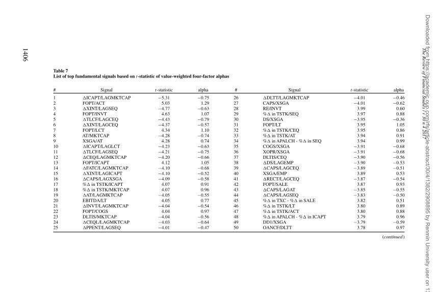
Similarly, Table 7 presents the top 100 signals based on the absolute value ofthe t-statistics of value-weighted four-factor alphas. The top-ranked signal onthis list is �ICAPT/LAGMKTCAP (change in total invested capital dividedby lagged market cap), with a t-statistic of −5.31. Again, many signals on thislist are new and have not been directly examined by prior studies, for example,�XINT/LAGSEQ (change in interest expense divided by lagged stockholders’equity), �TLCF/LAGCEQ (changes in tax loss carryforward divided by laggedcommon equity), and XSGA/AT (selling, general, and administrative expensedivided by total assets).
Taken together, Tables 6 and 7 reveal a number of new predictors for thecross-section of stock returns that cannot be explained by the Carhart (1997)four-factor model. We note that many significant fundamental signals are notincluded in Table 6 and Table 7 because of space constraints. For example, atotal of 549 signals have an equal-weighted four-factor alpha t-statistic thatis greater than 5 (in absolute value), while 362 signals have a value-weightedfour-factor alpha t-statistic greater than 3.
2.4.2 Economic drivers. What drives the predictive ability of the newfundamental signals identified in this study? We argue that these signalshave predictive ability for future returns because they contain value-relevantinformation about future firm performance and the market fails to impound thisinformation into stock prices in a timely manner.
One possible explanation for the delayed reaction to public accountinginformation is that transactions costs create an impediment to tradingand therefore prevent a complete and immediate response to accountinginformation. However, trading costs alone cannot explain the predictive ability
1403
Dow
nloaded from https://academ
ic.oup.com/rfs/article-abstract/30/4/1382/2908895 by R
enmin U
niversity user on 13 Novem
ber 2019
The
Review
ofFinancialStudies
/v30
n4
2017
Table 6List of top fundamental signals based on t-statistic of equal-weighted four-factor alphas
# Signal t-statistic alpha # Signal t-statistic alpha
1 �LT/LAGAT −8.91 −0.74 26 CEQ/MKTCAP 7.71 0.822 �LT/LAGICAPT −8.76 −0.74 27 �LT/LAGXSGA −7.68 −0.673 �LCT/LAGAT −8.75 −0.67 28 �XINT/LAGPPENT −7.67 −0.574 �LT/LAGCEQ −8.72 −0.74 29 �DCVT/LAGXSGA −7.65 −0.695 DLC/SALE −8.58 −0.66 30 AQS/SALE −7.65 −0.476 �XINT/LAGAT −8.57 −0.65 31 %� in XINT −7.63 −0.507 CEQT/MKTCAP 8.46 0.85 32 DLC/EMP −7.62 −0.548 DPACT/PPENT 8.38 0.89 33 �DLTT/LAGAT −7.62 −0.539 PPEGT/PPENT 8.38 0.89 34 �INVT/LAGCOGS −7.61 −0.7010 %� in PPENT −8.36 −0.83 35 DLC/COGS −7.61 −0.5711 DPVIEB/PPENT 8.34 1.03 36 NP/EMP −7.58 −0.4512 �LT/LAGSEQ −8.17 −0.72 37 �XINT/LAGCEQ −7.57 −0.6113 �INVT/LAGSALE −8.16 −0.74 38 AQS/XSGA −7.54 −0.5214 AQS/INVT −8.14 −0.51 39 �PPENT/LAGLT −7.54 −0.7215 �XINT/LAGXSGA −8.09 −0.63 40 CEQL/MKTCAP 7.54 0.8116 �LCT/LAGICAPT −8.07 −0.62 41 �DLTT/LAGPPENT −7.53 −0.4917 �XINT/LAGLT −8.01 −0.57 42 �AP/LAGACT −7.53 −0.8218 �LCT/LAGCEQ −7.95 −0.61 43 �AP/LAGCEQ −7.53 −0.8019 PPEVED/PPENT 7.92 0.84 44 �LCT/LAGSEQ −7.50 −0.5820 %� in LT −7.91 −0.66 45 �INVT/LAGPPENT −7.49 −0.6621 DLTIS/PPENT −7.83 −0.65 46 �LT/LAGLCT −7.49 −0.6422 �CSTK/LAGXSGA −7.78 −0.53 47 �LCT/LAGXSGA −7.48 −0.6123 �LT/LAGPPENT −7.77 −0.67 48 �XINT/LAGICAPT −7.46 −0.5924 �LCT/LAGACT −7.76 −0.58 49 SEQ/MKTCAP 7.46 0.7825 NP/SALE −7.76 −0.52 50 �INVT/LAGACT −7.46 −0.67
(continued )
1404
Dow
nloaded from https://academ
ic.oup.com/rfs/article-abstract/30/4/1382/2908895 by R
enmin U
niversity user on 13 Novem
ber 2019
Fundam
entalAnalysis
andthe
Cross-Section
ofStockR
eturns
Table 6Continued
# Signal t-statistic alpha # Signal t-statistic alpha
51 DLTIS/SALE −7.43 −0.73 76 �AP/LAGSEQ −7.08 −0.7652 DLC/ACT −7.41 −0.54 77 AQS/COGS −7.06 −0.4353 �PPENT/LAGAT −7.40 −0.77 78 �XINT/LAGACT −7.06 −0.5754 �INVT/LAGAT −7.39 −0.67 79 �AP/LAGAT −7.06 −0.7455 �DLC/LAGAT −7.38 −0.44 80 �INVT/LAGCEQ −7.05 −0.6456 �CSTK/LAGCEQ −7.34 −0.47 81 DLTIS/CEQ −7.05 −0.7257 DLTIS/AT −7.32 −0.71 82 �AT/LAGCEQ −7.04 −0.8558 �XINT/LAGSEQ −7.31 −0.58 83 AQS/ICAPT −7.04 −0.4459 DLTIS/ICAPT −7.31 −0.71 84 �CSTK/LAGICAPT −7.02 −0.4560 �DLTT/LAGICAPT −7.31 −0.51 85 %�LCT −7.02 −0.5661 �AP/LAGSALE −7.28 −0.82 86 �CSTK/LAGICAPT −7.00 −0.4862 �DLC/LAGPPENT −7.25 −0.43 87 DLTIS/SEQ −7.00 −0.7263 �INVT/LAGXSGA −7.23 −0.65 88 �XINT/LAGLCT −6.99 −0.5264 �AP/LAGCOGS −7.22 −0.81 89 �LCT/LAGPPENT −6.99 −0.5865 �PPENT/LAGICAPT −7.19 −0.74 90 %�INVT −6.98 −0.6866 �PPENT/LAGXSGA −7.18 −0.75 91 �LCT/LAGSALE −6.98 −0.5767 �PPENT/LAGCEQ −7.18 −0.75 92 AQS/LCT −6.98 −0.4668 �INVT/LAGLCT −7.17 −0.62 93 �CSTK/LAGSEQ −6.94 −0.4569 AQS/AT −7.17 −0.44 94 �LT/LAGACT −6.94 −0.6470 %�PPEGT −7.13 −0.66 95 SSTK/XSGA −6.94 −0.8071 �DLC/LAGLCT −7.13 −0.40 96 DVPIBB/MKTCAP 6.92 1.0172 �DLTT/LAGSEQ −7.12 −0.52 97 �DLTT/LAGCEQ −6.91 −0.5173 �CSTK/LAGACT −7.09 −0.50 98 DVPIBB/PPENT 6.91 0.9474 NP/COGS −7.08 −0.44 99 %�CSTK −6.91 −0.5675 DVPIBB/LT 7.08 0.99 100 �INVT/LAGLT −6.90 −0.59
Table 6 lists the top 100 fundamental signals ranked based on the absolute value of t-statistics of equal-weighted Carhart four-factor alphas. Our sample period is 1963–2013. Our sampleconsists of 18,113 fundamental signals constructed from the combination of 240 accounting variables and seventy-six financial ratios and configurations. At the end of June of year t , weform decile portfolios based on the value of each fundamental signal at the end of year t-1. We form the long-short portfolio based on the two extreme decile portfolios and hold them fortwelve months. We estimate four-factor alphas based on the Carhart (1997) model. Alphas are expressed in percent per month.1405
Dow
nloaded from https://academ
ic.oup.com/rfs/article-abstract/30/4/1382/2908895 by R
enmin U
niversity user on 13 Novem
ber 2019
The
Review
ofFinancialStudies
/v30
n4
2017
Table 7List of top fundamental signals based on t-statistic of value-weighted four-factor alphas
# Signal t-statistic alpha # Signal t-statistic alpha
1 �ICAPT/LAGMKTCAP −5.31 −0.75 26 �DLTT/LAGMKTCAP −4.01 −0.462 FOPT/ACT 5.03 1.29 27 CAPS/XSGA −4.01 −0.623 �XINT/LAGSEQ −4.77 −0.63 28 RE/INVT 3.99 0.604 FOPT/INVT 4.63 1.07 29 %� in TSTK/SEQ 3.97 0.885 �TLCF/LAGCEQ −4.43 −0.79 30 DS/XSGA −3.95 −0.366 �XINT/LAGCEQ −4.37 −0.57 31 FOPT/LT 3.95 1.057 FOPT/LCT 4.34 1.10 32 %� in TSTK/CEQ 3.95 0.868 AT/MKTCAP −4.28 −0.74 33 %� in TSTK/AT 3.94 0.919 XSGA/AT 4.28 0.74 34 %� in APALCH - %� in SEQ 3.94 0.9910 �ICAPT/LAGLCT −4.23 −0.63 35 COGS/XSGA −3.91 −0.6811 �TLCF/LAGSEQ −4.21 −0.75 36 XOPR/XSGA −3.91 −0.6812 �CEQ/LAGMKTCAP −4.20 −0.66 37 DLTIS/CEQ −3.90 −0.5613 FOPT/ICAPT 4.12 1.05 38 �DS/LAGEMP −3.90 −0.5314 �FATC/LAGMKTCAP −4.10 −0.68 39 �CAPS/LAGCEQ −3.89 −0.5115 �XINT/LAGICAPT −4.10 −0.52 40 XSGA/EMP 3.89 0.5316 �CAPS/LAGXSGA −4.09 −0.58 41 �RECT/LAGCEQ −3.87 −0.5417 %� in TSTK/ICAPT 4.07 0.91 42 FOPT/SALE 3.87 0.9318 %� in TSTK/MKTCAP 4.07 0.96 43 �CAPS/LAGAT −3.85 −0.5519 �AT/LAGMKTCAP −4.05 −0.55 44 �CAPS/LAGSEQ −3.83 −0.5020 EBITDA/LT 4.05 0.77 45 %� in TXC - %� in SALE 3.82 0.5121 �INVT/LAGMKTCAP −4.04 −0.54 46 %� in TSTK/LT 3.80 0.8922 FOPT/COGS 4.04 0.97 47 %� in TSTK/ACT 3.80 0.8823 DLTIS/MKTCAP −4.04 −0.56 48 %� in APALCH - %� in ICAPT 3.79 0.9624 �CEQL/LAGMKTCAP −4.03 −0.64 49 DD1/XSGA −3.79 −0.5925 �PPENT/LAGSEQ −4.01 −0.47 50 OANCF/DLTT 3.78 0.97
(continued )
1406
Dow
nloaded from https://academ
ic.oup.com/rfs/article-abstract/30/4/1382/2908895 by R
enmin U
niversity user on 13 Novem
ber 2019
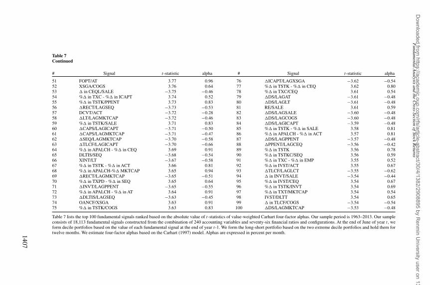
Fundam
entalAnalysis
andthe
Cross-Section
ofStockR
eturns
Table 7Continued
# Signal t-statistic alpha # Signal t-statistic alpha
51 FOPT/AT 3.77 0.96 76 �ICAPT/LAGXSGA −3.62 −0.5452 XSGA/COGS 3.76 0.64 77 %� in TSTK - %� in CEQ 3.62 0.8053 � in CEQL/SALE −3.75 −0.46 78 %� in TXC/CEQ 3.61 0.5454 %� in TXC - %� in ICAPT 3.74 0.52 79 �DS/LAGAT −3.61 −0.4855 %� in TSTK/PPENT 3.73 0.83 80 �DS/LAGLT −3.61 −0.4856 �RECT/LAGSEQ −3.73 −0.53 81 RE/SALE 3.61 0.5957 DCVT/ACT −3.72 −0.28 82 �DS/LAGSALE −3.60 −0.4858 �LT/LAGMKTCAP −3.72 −0.46 83 �DS/LAGCOGS −3.60 −0.4859 %� in TSTK/SALE 3.71 0.83 84 �DS/LAGICAPT −3.59 −0.4860 �CAPS/LAGICAPT −3.71 −0.50 85 %� in TSTK - %� in SALE 3.58 0.8161 �CAPS/LAGMKTCAP −3.71 −0.47 86 %� in APALCH - %� in ACT 3.57 0.8162 �SEQ/LAGMKTCAP −3.70 −0.58 87 �DS/LAGPPENT −3.57 −0.4863 �TLCF/LAGICAPT −3.70 −0.66 88 �PPENT/LAGCEQ −3.56 −0.4264 %� in APALCH - %� in CEQ 3.69 0.91 89 %� in TSTK 3.56 0.7865 DLTIS/SEQ −3.68 −0.54 90 %� in TSTKC/SEQ 3.56 0.5966 XINT/LT −3.67 −0.58 91 %� in TXC - %� in EMP 3.55 0.5267 %� in TSTK - %� in ACT 3.66 0.81 92 %� in IVST/ACT 3.55 0.6768 %� in APALCH-%� MKTCAP 3.65 0.94 93 �TLCF/LAGLCT −3.55 −0.6269 �RECT/LAGMKTCAP −3.65 −0.51 94 � in INVT/SALE −3.54 −0.4470 %� in TXPD - %� in SEQ 3.65 0.64 95 %� in IVST/CEQ 3.54 0.6771 �INVT/LAGPPENT −3.65 −0.55 96 %� in TSTK/INVT 3.54 0.6972 %� in APALCH - %� in AT 3.64 0.91 97 %� in TXT/MKTCAP 3.54 0.5473 �DLTIS/LAGSEQ −3.63 −0.45 98 IVST/DLTT 3.54 0.6574 OANCF/XSGA 3.63 0.91 99 � in TLCF/COGS −3.54 −0.5475 %� in TSTK/COGS 3.63 0.83 100 �DS/LAGMKTCAP −3.53 −0.48
Table 7 lists the top 100 fundamental signals ranked based on the absolute value of t-statistics of value-weighted Carhart four-factor alphas. Our sample period is 1963–2013. Our sampleconsists of 18,113 fundamental signals constructed from the combination of 240 accounting variables and seventy-six financial ratios and configurations. At the end of June of year t , weform decile portfolios based on the value of each fundamental signal at the end of year t-1. We form the long-short portfolio based on the two extreme decile portfolios and hold them fortwelve months. We estimate four-factor alphas based on the Carhart (1997) model. Alphas are expressed in percent per month.1407
Dow
nloaded from https://academ
ic.oup.com/rfs/article-abstract/30/4/1382/2908895 by R
enmin U
niversity user on 13 Novem
ber 2019
The Review of Financial Studies / v 30 n 4 2017
of our fundamental signals. This is due to the fact the fundamental-based tradingstrategies considered in our study are rebalanced once a year and therefore havevery low turnover rates. Untabulated results indicate that the average turnoverrate for our top fundamental signals is approximately 66% per year for bothlong and short portfolios. Using Novy-Marx and Velikov’s (2016) estimates ofround-trip trading costs, that is, between 0.76% and 1.63%,21 we find that thetotal trading costs for our strategies are between 1.01% and 2.15% per year.Tables 6 and 7 show that the alphas for most of our top fundamental signalsrange from 6% to 12% per year, far exceeding the estimated trading costs.
We contend that limited attention is a possible reason why investors fail tofully appreciate the information content of our fundamental signals. Investorshave limited attention and cognitive processing power. In the meantime,financial statement information is vast. Investors face a continuing stream offinancial reports for thousands of firms that contain hundreds of accountingvariables. Behavioral theory suggests that in the presence of limited attentioninvestors will not make full use of the available accounting information(Hirsheleifer et al. 2004). In particular, investors who face limited attention willtend to focus on more salient information while overlooking relatively obscurevariables such as interest expense and tax loss carryforward, thereby leadingto subsequent predictable returns associated with these accounting variables.
Having discussed at a general level why the new fundamental signals maybe systematically related to mispricing, we next provide a discussion on thespecific mechanisms why several prominent anomaly variables identified inthis study may predict future stock returns.
Interest expense. We find that changes in interest expense (XINT)scaled by several accounting variables including lagged total assets,common equity, and total invested capital are significant negativepredictors of future stock returns. An increase in interest expense maybe due to either an increase in the amount of debt or an increase inthe interest rate paid on the debt, or both. Debt issuance, to the extentthat it is used to finance asset growth that is motivated by “empirebuilding,” will tend to correlate negatively with future firm performance.An unexpected increase in the interest rate may indicate a deterioratingcredit environment and potential financial distress. If investors do notfully understand the information content of interest expense, a largeincrease in interest expense will tend to be associated with low futurestock returns.
Short-term debt. We find that the level of short-term debt (DLC) scaledby total sales, number of employees, and cost of goods sold are negative
21 These estimates are based on the implied round-trip trading costs of “low-turnover strategies” in Table 3 ofNovy-Marx and Velikov (2016). Their estimates are likely upper bounds. Frazzini, Israel, and Moskowitz (2015)report that the round-trip trading costs for a large institutional investor are a small fraction of those estimated byNovy-Marx and Velikov (2016).
1408
Dow
nloaded from https://academ
ic.oup.com/rfs/article-abstract/30/4/1382/2908895 by R
enmin U
niversity user on 13 Novem
ber 2019
Fundamental Analysis and the Cross-Section of Stock Returns
predictors of future stock returns. A disproportionately large amountof short-term debt may indicate a liquidity problem. Moreover, firmsface a rollover risk in short-term debt, particularly during financialcrises. If investors underestimate this rollover risk and the cost offinancial distress, the market will temporarily overvalue firms with adisproportionately large amount of short-term debt. When more publicinformation is released to the market in subsequent periods, these firmswill experience low/negative future stock returns.
Tax loss carryforward. We find that changes in tax loss carryforward(TLCF) scaled by various accounting variables negatively predict futurestock returns. The corporate income tax in the United States providestax relief to firms that report losses. Firms that have paid positive taxesduring the past three years may “carry back” their losses and receivea tax refund. Firms that exhaust their potential carrybacks must carrytheir losses forward.Afirm with a large increase in tax loss carryforwardmost likely has experienced persistent losses in past years. If investorsdo not fully understand the persistent nature of the firm’s losses, then anegative relation between changes in tax loss carryforward and futurestock returns may arise.
Selling, general, and administrative expense. Selling, general, andadministrative expense (XSGA) scaled by total assets, number ofemployees, and cost of goods sold are positive predictors of futurestock returns. Although XSGA is an expense, it generates current andfuture economic benefits that may be underestimated by investors.For example, XSGA includes marketing expense, which may correlatepositively with future sales. The XSGA also includes labor expense,which may be positively correlated with labor productivity. If the marketfails to impound such information into prices, then a high XSGA willtend to predict high future stock returns.
2.5 Robustness testsIn this section, we perform a number of robustness tests to ensure that ourresults are not sensitive to various sample and methodological choices.
2.5.1 Financial stocks. In our main analysis, we follow many previousstudies in the anomalies literature (e.g., Fama and French 2008) and excludefinancial stocks. To gauge the robustness of our results, we repeat our mainanalysis by including financial stocks in our sample. To conserve space, wereport the results of this analysis in Table IA.5 of the InternetAppendix. Overall,our results are similar to those reported in Table 1 and Table 2. That is, we findthat the superior performance of top-ranked fundamental signals cannot beexplained by random chance.
1409
Dow
nloaded from https://academ
ic.oup.com/rfs/article-abstract/30/4/1382/2908895 by R
enmin U
niversity user on 13 Novem
ber 2019
The Review of Financial Studies / v 30 n 4 2017
2.5.2 Fama and French five-factor alphas. Fama and French (2015) pro-pose a new five-factor model by adding a profitability factor and an investmentfactor to their workhorse three-factor model. We repeat our bootstrap analysison the t-statistics of Fama and French five-factor alphas and present the resultsin Table IA.7 in the Internet Appendix. Our results are qualitatively unchanged.
2.5.3 Alternative universe of signals. We repeat our analyses on severalalternative universes of fundamental signals. In particular, we find that ourresults are qualitatively similar when we impose more (or less) stringent datarequirements on the accounting variables (e.g., when we require a minimumof 500 or 2,000 average observations per year as opposed to 1,000). Moreover,because the number of listed firms changes over time, we also implement atime-varying minimum number of firms’ rule. Specifically, we require that thepercentage of firms with nonmissing data on an accounting variable be at least30% per year. Our results based on this alternative variable selection rule arevery similar to those contained in Table 1. We present the results of theserobustness tests in Table IA.8 of the Internet Appendix.
2.5.4 Industry-adjusted signals. One might argue that financial ratios areindustry specific, so it may be more meaningful to compare a firm’s financialratios to its industry peers. In Table IA.9 of the Internet Appendix, we subtractthe industry median from each firm’s fundamental signal before formingportfolios. We find essentially the same results when we use industry-adjustedsignals.
2.5.5 Sampling without replacement. In our main bootstrap analysis, wefollow the standard approach and draw simulated data with replacement. Analternative approach is to sample without replacement, which can be usedwhen drawing subsamples of size m<n from the original data (Horowitz 2001,3169).22 We perform a robustness test using this alternative sampling procedureand report the results in Table IA.10 of the InternetAppendix. Overall, our mainfindings are qualitatively unchanged.
2.5.6 International evidence. We also extend our analysis to internationalmarkets. We follow Novy-Marx (2013) and Frazzini and Pedersen (2014)and include the following nineteen developed countries in our sample:Australia, Austria, Belgium, Cananda, Denmark, Finland, France, Germany,Great Britain, Hong Kong, Italy, Japan, the Netherlands, New Zealand,Norway, Singapore, Spain, Sweden, and Switzerland. We obtain annualaccounting variables from Compustat North America (for Canadian firms) and
22 Drawing samples of the same size as the original data without replacement would imply that each observationis drawn exactly once, resulting in simulated samples that differ from the original data only in the order of eachobservation. As a result, there would be no variation in the mean return or alpha across simulated samples. Ourresults are based on drawing subsamples of thirty years (out of fifty years) without replacement.
1410
Dow
nloaded from https://academ
ic.oup.com/rfs/article-abstract/30/4/1382/2908895 by R
enmin U
niversity user on 13 Novem
ber 2019

Fundamental Analysis and the Cross-Section of Stock Returns
Compustat Global. Our analysis is based on 125 accounting variables and 8,143fundamental signals. This universe is smaller than that of the United Statesbecause of data availability. Our sample excludes financial firms, noncommonstocks, and low-priced stocks and covers the period from 1990 to 2013. Weremove extreme return observations by following the standard procedure ofInce and Porter (2003). We follow Hou, Karolyi, and Kho (2011) and sort stocksbased on each signal in two ways, across all countries (global) and within eachcountry (local). We compute returns in both U.S. dollar and local currency.Finally, we estimate alphas using global Fama-French factors downloadedfrom Kenneth French’s website. We report our results in Table IA.13 of theInternet Appendix. Overall, we find similar results to those in the United Stateswhen looking at equal-weighted portfolios. That is, the extreme percentilesof alphas and their t-statistics are too large to be explained by chance. Thevalue-weighted results, however, are much weaker than those for the UnitedStates. This is likely due to three reasons. First, the sample period for theinternational data is shorter. Second, there is a lot of noise in the internationaldata including the market capitalization data. Third, accounting variables acrossdifferent countries may not be completely comparable due to differences inaccounting rules and standards.
2.6 Past return–based anomaliesAlthough we focus on financial statement variables in this paper, our approachis general and can be applied to other categories of anomaly variables. Todemonstrate this generality, we apply our methodology to past return–basedanomalies.23 Similar to financial statement variables, past returns are also wellsuited for our analysis because although researchers have numerous choices onwhich past returns to use, we can construct a “universe” of past return signalsby using permutational arguments.
Previous studies have shown that past returns contain information aboutfuture stock returns. Both short- (one month) and long-term (three to five years)past returns are negatively associated with future returns, while intermediate-term (three to twelve months) past returns are positively related to future returns(DeBondt andThaler 1985; Jegadeesh 1990; Jegadeesh andTitman 1993). Morerecently, Novy-Marx (2012) shows that the intermediate momentum effect isprimarily driven by stock returns during twelve to seven months prior to theportfolio formation date, and Heston and Sadka (2008) document that paststock returns have significant predictive power for future returns during thesame calendar month. We evaluate the extent to which these past return–basedanomalies are due to random chance.
2.6.1 Construction of a universe. For ease of exposition, we denote eachpast return variable as the cumulative return between month t −k−j and month
23 We thank the referee for suggesting this analysis.
1411
Dow
nloaded from https://academ
ic.oup.com/rfs/article-abstract/30/4/1382/2908895 by R
enmin U
niversity user on 13 Novem
ber 2019
The Review of Financial Studies / v 30 n 4 2017
t −k−1, where t is the current month, j is the number of months in the formationperiod, and k is the number of months we skip between the end of the formationperiod and the start of the holding period. In our study, the possible values forj are from 1 to 240 (i.e., one month to twenty years). The possible values of k
are from 0 to 12 and then 24, 36, 48, and 60. Positive values of k allow us (i)to mitigate the effect of bid-ask bounce; (ii) to examine the predictive abilityof short-, intermediate-, and long-term returns independent of each other; and(iii) more generally, to consider any past return that is not adjacent to theholding period. Using all combinations of j and k, we are able to constructa “universe” of 4,080 past return–based anomaly variables. This “universe”includes the past return signals documented in prior literature, for example,RETt−1:t−1 (Jegadeesh 1990), RETt−6:t−1 (Jegadeesh and Titman 1993, 2001),RETt−12:t−2 (Fama and French 1996), RETt−60:t−13 (DeBondt and Thaler 1985),RETt−12:t−7 (Novy-Marx 2012), RETt−12:t−12 (Heston and Sadka 2008), as wellas numerous unreported and unpublished past return signals.
At each month t , we sort all stocks based on their past returns and form decileportfolios.24 We buy stocks in the highest past return decile and short stocksin the lowest past return decile. We rebalance our portfolios each month andhold them for one month. We compute long-short returns and then estimate theCAPM one-factor alphas and the Fama and French three-factor alphas of thelong-short returns. We focus on one- and three-factor alphas in this analysisbecause the Carhart four-factor model includes a momentum factor.
2.6.2 Top past return signals. In panel A of Table 8, we list the top signalsranked based on equal-weighted three-factor alpha t-statistics, separately forpositive and negative alphas. The left half of panel A, which reports the top 25positive predictors, indicates that most of these past return signals are over thethree- to twelve-month horizon, suggesting the intermediate-term momentumeffect of Jegadeesh and Titman (1993) is pervasive. The top-ranked signal isRETt−12:t−3, which has an alpha of 1.72% per month and a t-statistic of 6.27.We note that the past return variable examined by Novy-Marx (2012) is ranked#3 on this list, with an alpha of 1.32% per month and a t-statistic of 6.2.
The right half of panel A lists the top 25 past return signals that are negativelyrelated to future stock returns. Although all of these signals are long-termreturns, they are not necessarily within the time frame that prior studies haveexamined. Specifically, prior studies of long-run reversals have focused on thepast one- to five-year returns, that is, up to month t-60. However, most of thesignals on this list extend beyond the past five years. For example, the top-ranked past return variable is RETt−136:t−37, which is the cumulative returnover a 100-month period from month t-136 to month t-37. We dub this newfinding “long long-run reversal.”
24 We remove those stocks with a share price below $1 or in the smallest NYSE size decile at the portfolio formationdate.
1412
Dow
nloaded from https://academ
ic.oup.com/rfs/article-abstract/30/4/1382/2908895 by R
enmin U
niversity user on 13 Novem
ber 2019
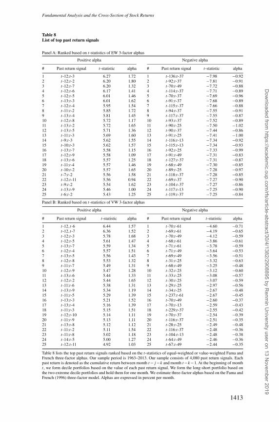
Fundamental Analysis and the Cross-Section of Stock Returns
Table 8List of top past return signals
Panel A: Ranked based on t-statistics of EW 3-factor alphas
Positive alpha Negative alpha
# Past return signal t-statistic alpha # Past return signal t-statistic alpha
1 t-12:t-3 6.27 1.72 1 t-136:t-37 −7.98 −0.922 t-12:t-2 6.20 1.80 2 t-92:t-37 −7.81 −0.913 t-12:t-7 6.20 1.32 3 t-70:t-49 −7.72 −0.884 t-12:t-6 6.17 1.41 4 t-114:t-37 −7.71 −0.895 t-12:t-5 6.01 1.46 5 t-70:t-37 −7.69 −0.966 t-13:t-3 6.01 1.62 6 t-91:t-37 −7.68 −0.897 t-12:t-4 5.95 1.54 7 t-115:t-37 −7.66 −0.888 t-11:t-2 5.85 1.72 8 t-94:t-37 −7.55 −0.919 t-13:t-4 5.81 1.45 9 t-117:t-37 −7.55 −0.8710 t-12:t-8 5.72 1.17 10 t-93:t-37 −7.52 −0.8911 t-13:t-2 5.72 1.65 11 t-90:t-25 −7.50 −1.0212 t-13:t-5 5.71 1.36 12 t-90:t-37 −7.44 −0.8613 t-11:t-3 5.69 1.60 13 t-91:t-25 −7.41 −1.0014 t-9:t-3 5.62 1.55 14 t-116:t-13 −7.34 −0.9215 t-10:t-3 5.62 1.57 15 t-115:t-13 −7.34 −0.9316 t-13:t-7 5.58 1.15 16 t-92:t-25 −7.33 −0.9917 t-12:t-9 5.58 1.09 17 t-91:t-49 −7.31 −0.8318 t-13:t-6 5.57 1.25 18 t-127:t-37 −7.31 −0.8719 t-11:t-4 5.57 1.46 19 t-68:t-49 −7.30 −0.8520 t-10:t-2 5.57 1.65 20 t-89:t-25 −7.28 −0.9721 t-7:t-2 5.56 1.58 21 t-118:t-37 −7.28 −0.8522 t-12:t-11 5.56 0.94 22 t-69:t-37 −7.27 −0.9023 t-9:t-2 5.54 1.62 23 t-104:t-37 −7.27 −0.8624 t-13:t-9 5.46 1.00 24 t-117:t-13 −7.25 −0.9025 t-6:t-2 5.43 1.25 25 t-119:t-37 −7.25 −0.84
Panel B: Ranked based on t-statistics of VW 3-factor alphas
Positive alpha Negative alpha
# Past return signal t-statistic alpha # Past return signal t-statistic alpha
1 t-12,t-6 6.44 1.57 1 t-70:t-61 −4.60 −0.712 t-12,t-7 6.36 1.52 2 t-69:t-61 −4.19 −0.653 t-12:t-3 5.78 1.68 3 t-70:t-49 −4.12 −0.594 t-12:t-5 5.61 1.47 4 t-68:t-61 −3.86 −0.615 t-13:t-7 5.59 1.34 5 t-71:t-61 −3.78 −0.596 t-12:t-4 5.57 1.51 6 t-71:t-49 −3.64 −0.537 t-13:t-5 5.56 1.43 7 t-69:t-49 −3.56 −0.518 t-12:t-8 5.53 1.32 8 t-31:t-25 −3.32 −0.639 t-11:t-7 5.49 1.31 9 t-68:t-49 −3.25 −0.4810 t-12:t-9 5.47 1.28 10 t-32:t-25 −3.12 −0.6011 t-13:t-6 5.44 1.33 11 t-33:t-25 −3.08 −0.5712 t-12:t-2 5.44 1.65 12 t-30:t-25 −3.07 −0.5913 t-11:t-6 5.38 1.31 13 t-29:t-25 −2.97 −0.5614 t-13:t-9 5.34 1.19 14 t-34:t-25 −2.67 −0.4815 t-11:t-5 5.29 1.39 15 t-237:t-61 −2.67 −0.4516 t-13:t-3 5.21 1.52 16 t-70:t-49 −2.60 −0.3717 t-13:t-4 5.16 1.39 17 t-70:t-13 −2.59 −0.4318 t-11:t-3 5.15 1.51 18 t-229:t-37 −2.55 −0.4219 t-12:t-10 5.14 1.11 19 t-70:t-37 −2.54 −0.3920 t-11:t-9 5.13 1.11 20 t-116:t-37 −2.51 −0.3521 t-13:t-8 5.12 1.12 21 t-28:t-25 −2.49 −0.4822 t-11:t-2 5.11 1.54 22 t-116:t-37 −2.48 −0.3623 t-11:t-8 5.02 1.18 23 t-104:t-13 −2.48 −0.3824 t-14:t-5 5.00 1.27 24 t-64:t-49 −2.46 −0.3625 t-12:t-11 4.92 1.03 25 t-67:t-49 −2.44 −0.35
Table 8 lists the top past return signals ranked based on the t-statistics of equal-weighted or value-weighted Fama andFrench three-factor alphas. Our sample period is 1963–2013. Our sample consists of 4,080 past return signals. Eachpast return is denoted as the cumulative return between month t −j −k and month t −k−1. At the beginning of montht , we form decile portfolios based on the value of each past return signal. We form the long-short portfolio based onthe two extreme decile portfolios and hold them for one month. We estimate three-factor alphas based on the Fama andFrench (1996) three-factor model. Alphas are expressed in percent per month.
1413
Dow
nloaded from https://academ
ic.oup.com/rfs/article-abstract/30/4/1382/2908895 by R
enmin U
niversity user on 13 Novem
ber 2019
The Review of Financial Studies / v 30 n 4 2017
The value-weighted results reported in panel B reveal essentially the samepattern. Return continuation signals concentrate on the three- to twelve-monthhorizon, while return reversal signals concentrate on much longer horizons,often beyond five years. We also note that although the momentum effectexhibits similar alphas and t-statistics between equal- and value-weightedreturns, the long-run reversal effect is significantly weaker when we examinevalue-weighted portfolios.
2.6.3 Bootstrap results. We conduct our bootstrap analysis on both alphasand t-statistics of alphas for our universe of past return signals. Table 9 presentsthe results. Panel A reports the results for t-statistics. Examining the t-statisticsof equal-weighted one-factor alphas, we find that the long-short performance ofpast return signals exhibit large t-statistics. For example, the 99th percentile oft-statistics is 4.34 and the 1st percentile is −7.87. The bootstrapped p-values formost extreme percentiles are less than 1%, indicating that the large t-statisticsat the extreme percentiles cannot be explained by sampling variation.25
The same qualitative results extend to the t-statistics of equal-weighed three-factor alphas and value-weighted one-factor alphas. However, the results forthe t-statistics of value-weighted three-factor alphas are somewhat different.We find that the distribution of t-statistics appears to have shifted upward aftercontrolling for the Fama and French factors. That is, the t-statistics at the 90th to100th percentiles have become more positive, while the t-statistics at the 0th to10th percentiles have become less negative. In fact, the bootstrapped p-valuescorresponding to the 1st to 10th percentiles are no longer below 5%. Thesefindings are consistent with Fama and French (1996), who find that their three-factor model helps explain the long-run reversal effect, and with Jegadeeshand Titman (2001), who show that the Fama and French three-factor modelexacerbates the momentum effect.
Panel B of Table 9 presents the bootstrap results for alphas. The resultsbasically mirror those contained in panel A. For example, the 99th percentileof equal-weighted one-factor alphas is 1.06% per month and the 1st percentileis −1.31% per month, both of which have a bootstrapped p-value of 0%.The value-weighted one-factor alpha results are similar. The 99th percentileof value-weighted one-factor alphas is 0.94% with a bootstrapped p-value of0.05%, and the 1st percentile is −0.81% with a bootstrapped p-value of 0.36%.These p-values indicate that, under the null hypothesis that all past returnstrategies are generating zero long-short returns, it is highly unlikely for us toobserve a 99th (1st) percentile of one-factor alpha that is more extreme than
25 We note that the p-values for the 90th to 97th percentiles are quite large (i.e., insignificant). This is becauseour universe of past return signals, by construction, is dominated by long-run past returns, which tend to havea negative relation with future stock returns. Table IA.14 of the Internet Appendix presents bootstrap results fora universe of past return signals that are all within the past sixty months. The positive and negative extremevalues of this alternative sample are much more symmetric. In particular, the 90th through 100th percentiles oft-statistics are all significant.
1414
Dow
nloaded from https://academ
ic.oup.com/rfs/article-abstract/30/4/1382/2908895 by R
enmin U
niversity user on 13 Novem
ber 2019
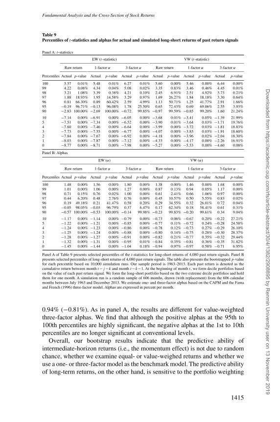
Fundamental Analysis and the Cross-Section of Stock Returns
Table 9Percentiles of t-statistics and alphas for actual and simulated long-short returns of past return signals
Panel A: t-statistics
EW (t-statistic) VW (t-statistic)
Raw return 1-factor α 3-factor α Raw return 1-factor α 3-factor α
Percentiles Actual p-value Actual p-value Actual p-value Actual p-value Actual p-value Actual p-value
100 5.57 0.01% 5.48 0.01% 6.27 0.01% 5.60 0.00% 5.46 0.00% 6.44 0.00%99 4.22 0.08% 4.34 0.04% 5.08 0.02% 3.35 0.83% 3.46 0.46% 4.45 0.01%98 3.21 1.08% 3.39 0.38% 4.21 0.10% 2.45 6.91% 2.51 4.92% 3.73 0.21%97 1.88 18.93% 1.95 14.58% 3.29 0.97% 1.69 26.27% 1.84 18.18% 3.30 0.64%96 0.81 66.30% 0.89 60.42% 2.59 4.99% 1.13 50.71% 1.25 41.77% 2.91 1.66%95 −0.19 96.71% −0.13 96.08% 1.78 25.50% 0.65 72.43% 0.69 69.06% 2.55 3.93%90 −2.83 100.00% −2.69 100.00% −0.72 99.85% −0.97 99.59% −0.85 99.20% 1.60 21.24%
10 −7.14 0.00% −6.91 0.00% −6.05 0.00% −3.68 0.01% −3.41 0.05% −1.39 21.99%5 −7.51 0.00% −7.34 0.00% −6.52 0.00% −3.90 0.01% −3.64 0.03% −1.71 19.76%4 −7.60 0.00% −7.46 0.00% −6.64 0.00% −3.99 0.00% −3.72 0.03% −1.81 18.83%3 −7.73 0.00% −7.55 0.00% −6.77 0.00% −4.07 0.00% −3.83 0.03% −1.91 18.60%2 −7.84 0.00% −7.67 0.00% −6.92 0.00% −4.18 0.00% −3.96 0.02% −2.04 18.30%1 −8.03 0.00% −7.87 0.00% −7.12 0.00% −4.33 0.00% −4.17 0.00% −2.26 16.91%0 −8.77 0.00% −8.71 0.00% −7.98 0.00% −5.27 0.00% −5.53 0.00% −4.60 0.08%
Panel B: Alphas
EW (α) VW (α)
Raw return 1-factor α 3-factor α Raw return 1-factor α 3-factor α
Percentiles Actual p-value Actual p-value Actual p-value Actual p-value Actual p-value Actual p-value
100 1.48 0.00% 1.56 0.00% 1.80 0.00% 1.38 0.00% 1.46 0.00% 1.68 0.00%99 1.01 0.00% 1.06 0.00% 1.27 0.00% 0.87 0.13% 0.94 0.05% 1.17 0.00%98 0.71 0.15% 0.76 0.02% 1.00 0.00% 0.61 2.41% 0.66 1.06% 0.97 0.00%97 0.44 6.20% 0.48 2.76% 0.76 0.00% 0.45 10.57% 0.50 5.55% 0.83 0.02%96 0.19 49.18% 0.21 41.47% 0.58 0.20% 0.29 34.55% 0.32 26.01% 0.72 0.04%95 −0.05 98.05% −0.03 96.79% 0.37 6.47% 0.17 62.34% 0.18 58.41% 0.61 0.31%90 −0.57 100.00% −0.53 100.00% −0.14 99.98% −0.23 99.83% −0.20 99.61% 0.34 9.04%
10 −1.17 0.00% −1.14 0.00% −0.79 0.00% −0.73 0.06% −0.67 0.20% −0.22 27.21%5 −1.22 0.00% −1.21 0.00% −0.85 0.00% −0.77 0.11% −0.72 0.24% −0.28 24.58%4 −1.24 0.00% −1.23 0.00% −0.86 0.00% −0.78 0.12% −0.73 0.27% −0.29 26.10%3 −1.25 0.00% −1.24 0.00% −0.88 0.00% −0.80 0.14% −0.75 0.28% −0.30 28.37%2 −1.28 0.00% −1.27 0.00% −0.91 0.00% −0.82 0.21% −0.77 0.35% −0.32 29.44%1 −1.32 0.00% −1.31 0.00% −0.95 0.01% −0.84 0.35% −0.81 0.36% −0.35 31.82%0 −1.45 0.00% −1.44 0.00% −1.04 0.18% −0.94 0.97% −0.97 0.58% −0.71 6.95%
Panel A of Table 9 presents selected percentiles of the t-statistics for long-short returns of 4,080 past return signals. Panel Bpresents selected percentiles of long-short returns of 4,080 past return signals. The table also presents the bootstrapped p-valuefor each percentile based on 10,000 simulation runs. Our sample period is 1963–2013. Each past return is denoted as thecumulative return between month t −j −k and month t −k−1. At the beginning of month t , we form decile portfolios basedon the value of each past return signal. We form the long-short portfolio based on the two extreme decile portfolios and holdthem for one month. A simulation run is a random sample of 606 months, drawn (with replacement) from the 606 calendarmonths between July 1963 and December 2013. We estimate one- and three-factor alphas based on the CAPM and the Famaand French (1996) three-factor model. Alphas are expressed in percent per month.
0.94% (−0.81%). As in panel A, the results are different for value-weightedthree-factor alphas. We find that although the positive alphas at the 95th to100th percentiles are highly significant, the negative alphas at the 1st to 10thpercentiles are no longer significant at conventional levels.
Overall, our bootstrap results indicate that the predictive ability ofintermediate-horizon returns (i.e., the momentum effect) is not due to randomchance, whether we examine equal- or value-weighed returns and whether weuse a one- or three-factor model as the benchmark model. The predictive abilityof long-term returns, on the other hand, is sensitive to the portfolio weighting
1415
Dow
nloaded from https://academ
ic.oup.com/rfs/article-abstract/30/4/1382/2908895 by R
enmin U
niversity user on 13 Novem
ber 2019
The Review of Financial Studies / v 30 n 4 2017
scheme and benchmark model. When we use the CAPM one-factor model orexamine equal-weighted returns, this predictive ability is highly significantand robust to sampling variation. However, when we use the Fama and Frenchthree-factor model combined with value-weighted returns, we cannot reject thehypothesis the predictive ability of long-term returns is attributed to randomchance for most extreme percentiles.
3. Conclusions
Previous studies have documented hundreds of cross-sectional returnanomalies. These anomalies have largely been evaluated without accounting forthe extensive search leading up to their discoveries. In this paper, we examinethe data-mining bias in cross-sectional return anomalies by constructing a“universe” of over 18,000 fundamental signals from financial statements andby using a bootstrap procedure.
We find that a large number of fundamental signals are significant predictorsof cross-sectional stock returns even after accounting for data mining.This predictive ability is more pronounced among small, low-institutionalownership, low-analyst coverage, and high-idiosyncratic volatility stocks. Wealso find that the long-short returns associated with fundamental signals aresignificantly higher following high-sentiment periods. These results suggestthat fundamental-based anomalies are more likely to result from mispricing. Wedemonstrate the generality of our approach by applying it to past return–basedanomaly variables. We show that the intermediate-term momentum effect isextremely robust to sampling variation, while the long-run reversal is somewhatsensitive to portfolio weighting schemes and benchmark models. Although weexamine both fundamental signals and past return signals, we acknowledgethat our analysis does not account for all the anomaly variables documentedin the literature (e.g., analyst forecast dispersion, governance index, breadthof ownership, political contribution, and media coverage). Future researchcan extend our framework and conduct a more comprehensive data-miningexercise.
1416
Dow
nloaded from https://academ
ic.oup.com/rfs/article-abstract/30/4/1382/2908895 by R
enmin U
niversity user on 13 Novem
ber 2019
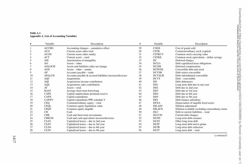
Fundam
entalAnalysis
andthe
Cross-Section
ofStockR
eturns
Table A.1Appendix A. List of Accounting Variables
# Variable Description # Variable Description
1 ACCHG Accounting changes – cumulative effect 29 COGS Cost of goods sold2 ACO Current assets other total 30 CSTK Common/ordinary stock (capital)3 ACOX Current assets other sundry 31 CSTKCV Common stock-carrying value4 ACT Current assets – total 32 CSTKE Common stock equivalents – dollar savings5 AM Amortization of intangibles 33 DC Deferred charges6 AO Assets – other 34 DCLO Debt capitalized lease obligations7 AOLOCH Assets and liabilities other net change 35 DCOM Deferred compensation8 AOX Assets – other – sundry 36 DCPSTK Convertible debt and stock9 AP Accounts payable – trade 37 DCVSR Debt senior convertible10 APALCH Accounts payable & accrued liabilities increase/decrease 38 DCVSUB Debt subordinated convertible11 AQC Acquisitions 39 DCVT Debt – convertible12 AQI Acquisitions income contribution 40 DD Debt debentures13 AQS Acquisitions sales contribution 41 DD1 Long-term debt due in one year14 AT Assets – total 42 DD2 Debt due in 2nd year15 BAST Average short-term borrowing 43 DD3 Debt due in 3rd year16 CAPS Capital surplus/share premium reserve 44 DD4 Debt due in 4th year17 CAPX Capital expenditure 45 DD5 Debt due in 5th year18 CAPXV Capital expenditure PPE schedule V 46 DFS Debt finance subsidiary19 CEQ Common/ordinary equity – total 47 DFXA Depreciation of tangible fixed assets20 CEQL Common equity liquidation value 48 DILADJ Dilution adjustment21 CEQT Common equity tangible 49 DILAVX Dilution available excluding extraordinary items22 CH Cash 50 DLC Debt in current liabilities – total23 CHE Cash and short-term investments 51 DLCCH Current debt changes24 CHECH Cash and cash equivalents increase/decrease 52 DLTIS Long-term debt issuance25 CLD2 Capitalized leases – due in 2nd year 53 DLTO Other long-term debt26 CLD3 Capitalized leases – due in 3rd year 54 DLTP Long-term debt tied to prime27 CLD4 Capitalized leases – due in 4th year 55 DLTR Long-term debt reduction28 CLD5 Capitalized leases – due in 5th year 56 DLTT Long-term debt – total
(continued )1417
Dow
nloaded from https://academ
ic.oup.com/rfs/article-abstract/30/4/1382/2908895 by R
enmin U
niversity user on 13 Novem
ber 2019
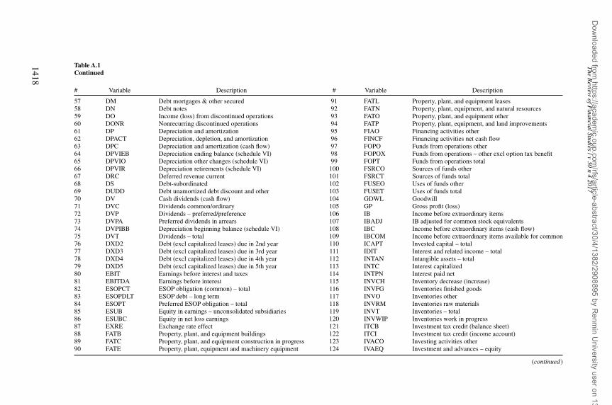
The
Review
ofFinancialStudies
/v30
n4
2017
Table A.1Continued
# Variable Description # Variable Description
57 DM Debt mortgages & other secured 91 FATL Property, plant, and equipment leases58 DN Debt notes 92 FATN Property, plant, equipment, and natural resources59 DO Income (loss) from discontinued operations 93 FATO Property, plant, and equipment other60 DONR Nonrecurring discontinued operations 94 FATP Property, plant, equipment, and land improvements61 DP Depreciation and amortization 95 FIAO Financing activities other62 DPACT Depreciation, depletion, and amortization 96 FINCF Financing activities net cash flow63 DPC Depreciation and amortization (cash flow) 97 FOPO Funds from operations other64 DPVIEB Depreciation ending balance (schedule VI) 98 FOPOX Funds from operations – other excl option tax benefit65 DPVIO Depreciation other changes (schedule VI) 99 FOPT Funds from operations total66 DPVIR Depreciation retirements (schedule VI) 100 FSRCO Sources of funds other67 DRC Deferred revenue current 101 FSRCT Sources of funds total68 DS Debt-subordinated 102 FUSEO Uses of funds other69 DUDD Debt unamortized debt discount and other 103 FUSET Uses of funds total70 DV Cash dividends (cash flow) 104 GDWL Goodwill71 DVC Dividends common/ordinary 105 GP Gross profit (loss)72 DVP Dividends – preferred/preference 106 IB Income before extraordinary items73 DVPA Preferred dividends in arrears 107 IBADJ IB adjusted for common stock equivalents74 DVPIBB Depreciation beginning balance (schedule VI) 108 IBC Income before extraordinary items (cash flow)75 DVT Dividends – total 109 IBCOM Income before extraordinary items available for common76 DXD2 Debt (excl capitalized leases) due in 2nd year 110 ICAPT Invested capital – total77 DXD3 Debt (excl capitalized leases) due in 3rd year 111 IDIT Interest and related income – total78 DXD4 Debt (excl capitalized leases) due in 4th year 112 INTAN Intangible assets – total79 DXD5 Debt (excl capitalized leases) due in 5th year 113 INTC Interest capitalized80 EBIT Earnings before interest and taxes 114 INTPN Interest paid net81 EBITDA Earnings before interest 115 INVCH Inventory decrease (increase)82 ESOPCT ESOP obligation (common) – total 116 INVFG Inventories finished goods83 ESOPDLT ESOP debt – long term 117 INVO Inventories other84 ESOPT Preferred ESOP obligation – total 118 INVRM Inventories raw materials85 ESUB Equity in earnings – unconsolidated subsidiaries 119 INVT Inventories – total86 ESUBC Equity in net loss earnings 120 INVWIP Inventories work in progress87 EXRE Exchange rate effect 121 ITCB Investment tax credit (balance sheet)88 FATB Property, plant, and equipment buildings 122 ITCI Investment tax credit (income account)89 FATC Property, plant, and equipment construction in progress 123 IVACO Investing activities other90 FATE Property, plant, equipment and machinery equipment 124 IVAEQ Investment and advances – equity
(continued )
1418
Dow
nloaded from https://academ
ic.oup.com/rfs/article-abstract/30/4/1382/2908895 by R
enmin U
niversity user on 13 Novem
ber 2019
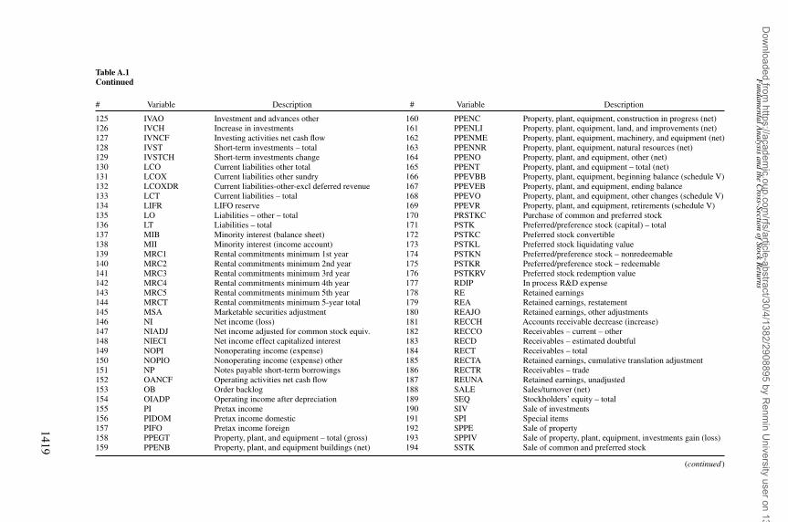
Fundam
entalAnalysis
andthe
Cross-Section
ofStockR
eturns
Table A.1Continued
# Variable Description # Variable Description
125 IVAO Investment and advances other 160 PPENC Property, plant, equipment, construction in progress (net)126 IVCH Increase in investments 161 PPENLI Property, plant, equipment, land, and improvements (net)127 IVNCF Investing activities net cash flow 162 PPENME Property, plant, equipment, machinery, and equipment (net)128 IVST Short-term investments – total 163 PPENNR Property, plant, equipment, natural resources (net)129 IVSTCH Short-term investments change 164 PPENO Property, plant, and equipment, other (net)130 LCO Current liabilities other total 165 PPENT Property, plant, and equipment – total (net)131 LCOX Current liabilities other sundry 166 PPEVBB Property, plant, equipment, beginning balance (schedule V)132 LCOXDR Current liabilities-other-excl deferred revenue 167 PPEVEB Property, plant, and equipment, ending balance133 LCT Current liabilities – total 168 PPEVO Property, plant, and equipment, other changes (schedule V)134 LIFR LIFO reserve 169 PPEVR Property, plant, and equipment, retirements (schedule V)135 LO Liabilities – other – total 170 PRSTKC Purchase of common and preferred stock136 LT Liabilities – total 171 PSTK Preferred/preference stock (capital) – total137 MIB Minority interest (balance sheet) 172 PSTKC Preferred stock convertible138 MII Minority interest (income account) 173 PSTKL Preferred stock liquidating value139 MRC1 Rental commitments minimum 1st year 174 PSTKN Preferred/preference stock – nonredeemable140 MRC2 Rental commitments minimum 2nd year 175 PSTKR Preferred/preference stock – redeemable141 MRC3 Rental commitments minimum 3rd year 176 PSTKRV Preferred stock redemption value142 MRC4 Rental commitments minimum 4th year 177 RDIP In process R&D expense143 MRC5 Rental commitments minimum 5th year 178 RE Retained earnings144 MRCT Rental commitments minimum 5-year total 179 REA Retained earnings, restatement145 MSA Marketable securities adjustment 180 REAJO Retained earnings, other adjustments146 NI Net income (loss) 181 RECCH Accounts receivable decrease (increase)147 NIADJ Net income adjusted for common stock equiv. 182 RECCO Receivables – current – other148 NIECI Net income effect capitalized interest 183 RECD Receivables – estimated doubtful149 NOPI Nonoperating income (expense) 184 RECT Receivables – total150 NOPIO Nonoperating income (expense) other 185 RECTA Retained earnings, cumulative translation adjustment151 NP Notes payable short-term borrowings 186 RECTR Receivables – trade152 OANCF Operating activities net cash flow 187 REUNA Retained earnings, unadjusted153 OB Order backlog 188 SALE Sales/turnover (net)154 OIADP Operating income after depreciation 189 SEQ Stockholders’ equity – total155 PI Pretax income 190 SIV Sale of investments156 PIDOM Pretax income domestic 191 SPI Special items157 PIFO Pretax income foreign 192 SPPE Sale of property158 PPEGT Property, plant, and equipment – total (gross) 193 SPPIV Sale of property, plant, equipment, investments gain (loss)159 PPENB Property, plant, and equipment buildings (net) 194 SSTK Sale of common and preferred stock
(continued )
1419
Dow
nloaded from https://academ
ic.oup.com/rfs/article-abstract/30/4/1382/2908895 by R
enmin U
niversity user on 13 Novem
ber 2019
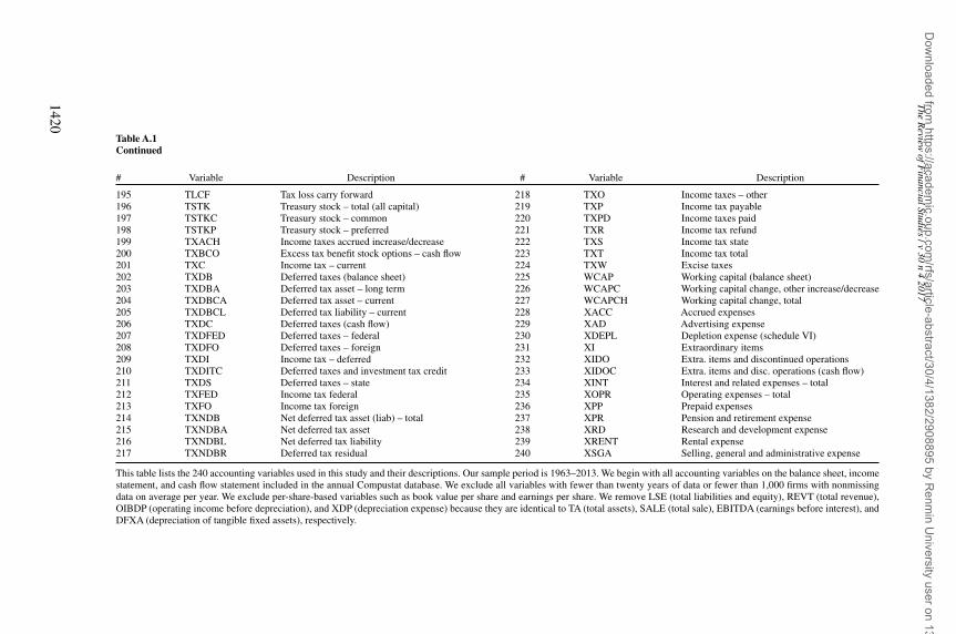
The
Review
ofFinancialStudies
/v30
n4
2017
Table A.1Continued
# Variable Description # Variable Description
195 TLCF Tax loss carry forward 218 TXO Income taxes – other196 TSTK Treasury stock – total (all capital) 219 TXP Income tax payable197 TSTKC Treasury stock – common 220 TXPD Income taxes paid198 TSTKP Treasury stock – preferred 221 TXR Income tax refund199 TXACH Income taxes accrued increase/decrease 222 TXS Income tax state200 TXBCO Excess tax benefit stock options – cash flow 223 TXT Income tax total201 TXC Income tax – current 224 TXW Excise taxes202 TXDB Deferred taxes (balance sheet) 225 WCAP Working capital (balance sheet)203 TXDBA Deferred tax asset – long term 226 WCAPC Working capital change, other increase/decrease204 TXDBCA Deferred tax asset – current 227 WCAPCH Working capital change, total205 TXDBCL Deferred tax liability – current 228 XACC Accrued expenses206 TXDC Deferred taxes (cash flow) 229 XAD Advertising expense207 TXDFED Deferred taxes – federal 230 XDEPL Depletion expense (schedule VI)208 TXDFO Deferred taxes – foreign 231 XI Extraordinary items209 TXDI Income tax – deferred 232 XIDO Extra. items and discontinued operations210 TXDITC Deferred taxes and investment tax credit 233 XIDOC Extra. items and disc. operations (cash flow)211 TXDS Deferred taxes – state 234 XINT Interest and related expenses – total212 TXFED Income tax federal 235 XOPR Operating expenses – total213 TXFO Income tax foreign 236 XPP Prepaid expenses214 TXNDB Net deferred tax asset (liab) – total 237 XPR Pension and retirement expense215 TXNDBA Net deferred tax asset 238 XRD Research and development expense216 TXNDBL Net deferred tax liability 239 XRENT Rental expense217 TXNDBR Deferred tax residual 240 XSGA Selling, general and administrative expense
This table lists the 240 accounting variables used in this study and their descriptions. Our sample period is 1963–2013. We begin with all accounting variables on the balance sheet, incomestatement, and cash flow statement included in the annual Compustat database. We exclude all variables with fewer than twenty years of data or fewer than 1,000 firms with nonmissingdata on average per year. We exclude per-share-based variables such as book value per share and earnings per share. We remove LSE (total liabilities and equity), REVT (total revenue),OIBDP (operating income before depreciation), and XDP (depreciation expense) because they are identical to TA (total assets), SALE (total sale), EBITDA (earnings before interest), andDFXA (depreciation of tangible fixed assets), respectively.
1420
Dow
nloaded from https://academ
ic.oup.com/rfs/article-abstract/30/4/1382/2908895 by R
enmin U
niversity user on 13 Novem
ber 2019
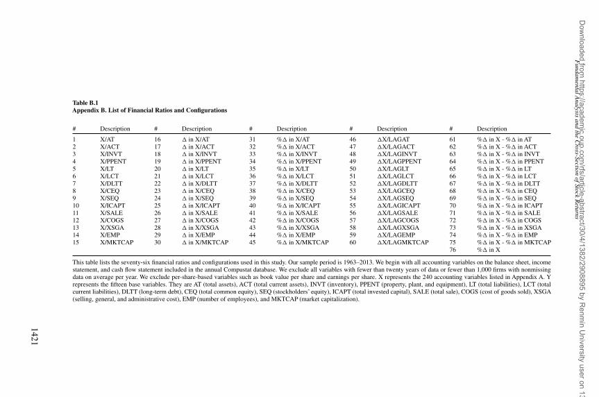
Fundam
entalAnalysis
andthe
Cross-Section
ofStockR
eturns
Table B.1Appendix B. List of Financial Ratios and Configurations
# Description # Description # Description # Description # Description
1 X/AT 16 � in X/AT 31 %� in X/AT 46 �X/LAGAT 61 %� in X - %� in AT2 X/ACT 17 � in X/ACT 32 %� in X/ACT 47 �X/LAGACT 62 %� in X - %� in ACT3 X/INVT 18 � in X/INVT 33 %� in X/INVT 48 �X/LAGINVT 63 %� in X - %� in INVT4 X/PPENT 19 � in X/PPENT 34 %� in X/PPENT 49 �X/LAGPPENT 64 %� in X - %� in PPENT5 X/LT 20 � in X/LT 35 %� in X/LT 50 �X/LAGLT 65 %� in X - %� in LT6 X/LCT 21 � in X/LCT 36 %� in X/LCT 51 �X/LAGLCT 66 %� in X - %� in LCT7 X/DLTT 22 � in X/DLTT 37 %� in X/DLTT 52 �X/LAGDLTT 67 %� in X - %� in DLTT8 X/CEQ 23 � in X/CEQ 38 %� in X/CEQ 53 �X/LAGCEQ 68 %� in X - %� in CEQ9 X/SEQ 24 � in X/SEQ 39 %� in X/SEQ 54 �X/LAGSEQ 69 %� in X - %� in SEQ10 X/ICAPT 25 � in X/ICAPT 40 %� in X/ICAPT 55 �X/LAGICAPT 70 %� in X - %� in ICAPT11 X/SALE 26 � in X/SALE 41 %� in X/SALE 56 �X/LAGSALE 71 %� in X - %� in SALE12 X/COGS 27 � in X/COGS 42 %� in X/COGS 57 �X/LAGCOGS 72 %� in X - %� in COGS13 X/XSGA 28 � in X/XSGA 43 %� in X/XSGA 58 �X/LAGXSGA 73 %� in X - %� in XSGA14 X/EMP 29 � in X/EMP 44 %� in X/EMP 59 �X/LAGEMP 74 %� in X - %� in EMP15 X/MKTCAP 30 � in X/MKTCAP 45 %� in X/MKTCAP 60 �X/LAGMKTCAP 75 %� in X - %� in MKTCAP
76 %� in X
This table lists the seventy-six financial ratios and configurations used in this study. Our sample period is 1963–2013. We begin with all accounting variables on the balance sheet, incomestatement, and cash flow statement included in the annual Compustat database. We exclude all variables with fewer than twenty years of data or fewer than 1,000 firms with nonmissingdata on average per year. We exclude per-share-based variables such as book value per share and earnings per share. X represents the 240 accounting variables listed in Appendix A. Yrepresents the fifteen base variables. They are AT (total assets), ACT (total current assets), INVT (inventory), PPENT (property, plant, and equipment), LT (total liabilities), LCT (totalcurrent liabilities), DLTT (long-term debt), CEQ (total common equity), SEQ (stockholders’ equity), ICAPT (total invested capital), SALE (total sale), COGS (cost of goods sold), XSGA(selling, general, and administrative cost), EMP (number of employees), and MKTCAP (market capitalization).
1421
Dow
nloaded from https://academ
ic.oup.com/rfs/article-abstract/30/4/1382/2908895 by R
enmin U
niversity user on 13 Novem
ber 2019

The Review of Financial Studies / v 30 n 4 2017
References
Baker, M., and J. Wurgler. 2006. Investor sentiment and the cross-section of stock returns. Journal of Finance61:1645–80.
Carhart, M. 1997. On persistence in mutual fund performance. Journal of Finance 52:57–82.
Chan, K., L. Chan, N. Jegadeesh, and L. Lakonishok. 2006. Earnings quality and stock returns. Journal ofBusiness 79:1041–82.
Chordia, T., and L. Shivakumar. 2002. Momentum, business cycle, and time-varying expected returns. Journalof Finance 57:985–19.
Cochrane, J. 2004. Asset Pricing. Princeton, NJ: Princeton University Press.
Conrad, J., and G. Kaul. 1998. An anatomy of trading strategies. Review of Financial Studies 11:489–519.
Cooper, M., H. Gulen, and M. Schill. 2008. Asset growth and the cross-section of stock returns. Journal ofFinance 63:1609–51.
DeBondt, W., and R. Thaler. 1985, Does stock market overreact? Journal of Finance 40:793–808.
Eisfeldt,A. L., and D. Papanikolaou. 2013. Organization capital and the cross-section of expected returns. Journalof Finance 68:1365–406.
Fama, E. F., and K. R. French. 1993. Common risk factors in the returns on stocks and bonds. Journal of FinancialEconomics 33:3–56.
———. 1996. Multifactor explanations of asset pricing anomalies. Journal of Finance 51:55–84.
———. 2008. Dissecting anomalies. Journal of Finance 63:1653–78.
———. 2010. Luck versus skill in the cross section of mutual fund returns. Journal of Finance 65:1915–47.
———. 2015. A five-factor asset pricing model. Journal of Financial Economics 116:1–22.
———. 2016. Dissecting anomalies with a five-factor model. Review of Financial Studies 29:69–103.
Foster, F. D., T. Smith, and R. E. Whaley. 1997.Assessing goodness-of-fit of asset pricing models: The distributionof the maximal R2. Journal of Finance 52:591–607.
Frazzini, A., R. Israel, and T. Moskowitz. 2015. Trading costs of asset pricing anomalies. Working Paper,University of Chicago.
Frazzini, A., and L. Pedersen. 2014. Betting against beta. Journal of Financial Economics 111:1–25.
Green, J., J. Hand, and X. Zhang. 2013. The supraview of return predictive signals. Review of Accounting Studies18:692–730.
———. 2014. The remarkable multidimensionality in the cross section of expected US stock returns. WorkingPaper, Pennsylvania State University.
Harvey, C., Y. Liu, and H. Zhu. 2016. …and the cross-section of stock returns. Review of Financial Studies29:5–68.
Heston, S, and R. Sadka. 2008. Seasonality in the cross-section of stock returns. Journal of Financial Economics87:418–45.
Hirshleifer, D., K. Hou, S. H. Teoh, and Y. Zhang. 2004. Do investors overvalue firms with bloated balancesheets? Journal of Accounting and Economics 38:297–331.
Horowitz, J. 2001. The bootstrap. In Handbook of Econometrics 5, ed. J. J. Heckman and E. Leamer, 3159–228.Amsterdam, the Netherlands: Elsevier.
Hou, K., A. Karolyi, and B. Kho. 2011. What factors drive global stock returns? Review of Financial Studies24:2527–74.
1422
Dow
nloaded from https://academ
ic.oup.com/rfs/article-abstract/30/4/1382/2908895 by R
enmin U
niversity user on 13 Novem
ber 2019

Fundamental Analysis and the Cross-Section of Stock Returns
Hou, K., C. Xue, and L. Zhang. 2015. Digesting anomalies: An investment approach. Review of Financial Studies28:650–705.
Ince, O., and R. Porter. 2003. Individual equity return data from Thomson Datastream: Handle with Care! Journalof Financial Research 29:463–79.
Jegadeesh, N. 1990. Evidence of predictable behavior of security returns. Journal of Finance 45:881–98.
Jegadeesh, N., and S. Titman. 1993. Returns to buying winners and selling losers: Implications for stock marketefficiency. Journal of Finance 48:65–91.
———. 2001. Profitability of momentum strategies:An evaluation of alternative explanations. Journal of Finance56:699–720.
———. 2002. Cross-sectional and time-series determinants of momentum returns. Review of Financial Studies15:143–57.
Karolyi, A., and B. Kho. 2004. Momentum strategies: Some bootstrap tests. Journal of Empirical Finance11:509–36.
Kosowski, R., A. Timmermann, R. Wermers, and H. White. 2006. Can mutual fund “stars” really pick stocks?New evidence from a Bootstrap analysis. Journal of Finance 61:2551–95.
Lev, B., and S. R. Thiagarajan. 1993. Fundamental information analysis. Journal of Accounting Research 31:190–215.
Lo, A., and C. Mackinlay. 1990. Data-snooping biases in tests of financial asset pricing models. Review ofFinancial Studies 3:431–67.
McLean, R., and J. Pontiff. 2016. Does academic research destroy stock return predictability? Journal of Finance71:5–31.
Merton, R. 1987. On the state of the efficient market hypothesis in financial economics. In Macroeconomics andFinance: Essays in Honor of Franco Modigliani, 93–124. Cambridge, MA: MIT Press.
Novy-Marx, R. 2012. Is momentum really momentum? Journal of Financial Economics 103:429–53.
———. 2013. The other side of value: The gross profitability premium. Journal of Financial Economics 108:1–28.
Novy-Marx, R., and M. Velikov. 2016. A taxonomy of anomalies and their trading costs. Review of FinancialStudies 29:104–47.
Ou, J. A., and S. H. Penman. 1989. Financial statement analysis and the prediction of stock returns. Journal ofAccounting and Economics 11:295–329.
Piotroski, J. D. 2000. Value investing: The use of historical financial statement information to separate winnersfrom losers. Journal of Accounting Research 38:1–41.
Pontiff, J. 2006. Costly arbitrage and the myth of idiosyncratic risk. Journal of Accounting and Economics42:35–52.
Shleifer, A., and R. W. Vishny. 1997. The limits of arbitrage. Journal of Finance 52:35–55.
Stambaugh, R., J. Yu, and Y. Yuan. 2012. The short of it: Investor sentiment and anomalies. Journal of FinancialEconomics 104:288–302.
Sullivan, R., A. Timmermann, and H. White. 1999. Data-snooping, technical trading rule performance, and thebootstrap. Journal of Finance 54:1647–91.
———. 2001. Dangers of data mining: The case of calendar effects in stock returns. Journal of Econometrics105:249–86.
Thomas, J., and H. Zhang. 2002. Inventory changes and future returns. Review and Accounting Studies 7:163–87.
White, H. 2000. A reality check for data snooping. Econometrica 68:1097–126.
1423
Dow
nloaded from https://academ
ic.oup.com/rfs/article-abstract/30/4/1382/2908895 by R
enmin U
niversity user on 13 Novem
ber 2019


![Fundamental Analysis and the Cross-Section of Stock Returns: A Data-Mining · PDF file · 2017-02-21[18:22 10/2/2017 RFS-hhx001.tex] Page: 3 1–42 Fundamental Analysis and the Cross-Section](https://img.pdfslide.us/doc/110x75/5abde52c7f8b9ad8278c75ec/fundamental-analysis-and-the-cross-section-of-stock-returns-a-data-mining-1822.jpg)