Fundamental Analysis and the Cross-Section of Stock Returns: A Data-Mining Approach

Abstract A key challenge to evaluate data-mining bias in stock return anomalies is that we do not observe all the variables considered by researchers. We overcome this challenge by constructing a “universe” of fundamental signals from financial statements and by using a bootstrap approach to measure the impact of data mining. We find that many fundamental signals are significant predictors of cross-sectional stock returns even after accounting for data mining. This predictive ability is more pronounced following high-sentiment periods, during earnings-announcement days, and among stocks with greater limits-to-arbitrage. Our evidence suggests that fundamental-based anomalies are not a product of data mining, and they are best explained by mispricing. Our approach is general and can be applied to other categories of anomaly variables.

October 2015

1

“Economists place a premium on the discovery of puzzles, which in the context at hand amounts to finding apparent rejections of a widely accepted theory of stock market behavior.”

Merton (1987, p. 104)

1. Introduction

Finance researchers have devoted a considerable amount of time and effort to searching

for stock return patterns that cannot be explained by traditional asset pricing models. As a result

of these efforts, there is now a large body of literature reporting hundreds of cross-sectional return

anomalies (Green, Hand, and Zhang (2013), Harvey, Liu, and Zhu (HLZ 2014), and McLean and

Pontiff (2014)). An important debate in the literature is whether the abnormal returns documented

in these studies are compensation for systematic risk, evidence of market inefficiency, or simply

the result of extensive data mining.

Data-mining concern arises because “the more scrutiny a collection of data is subjected to,

the more likely will interesting (spurious) patterns emerge” (Lo and MacKinlay (1990, p.432)).

Intuitively, if enough variables are considered, then by pure chance some of these variables will

generate abnormal returns even if they do not genuinely have any predictive ability for future stock

returns. Lo and MacKinlay contend that the degree of data mining bias increases with the number

of studies published on the topic. The cross section of stock returns is arguably the most researched

and published topic in finance; hence, the potential for spurious findings is also the greatest.

Although researchers have long recognized the potential danger of data mining, few studies

have examined its impact on a broad set of cross-sectional stock return anomalies.1 The lack of

research in this area is in part because of the difficulty to account for all the anomaly variables that

have been considered by researchers. Although one can easily identify published variables, one

1 The exceptions are HLZ (2014) and McLean and Pontiff (2014). We note that many papers have examined the impact of data mining on individual anomalies (e.g., Jegadeesh and Titman (2001)).

2

cannot observe the numerous variables that have been tried but not published or reported due to

the “publication bias.”2 In this paper, we overcome this challenge by examining a large and

important class of anomaly variables, i.e., fundamental-based variables, for which a “universe”

can be reasonably constructed.

We focus on fundamental-based variables, i.e., variables derived from financial statements,

for several reasons. First, many prominent anomalies such as the asset growth anomaly (Cooper,

Gulen, and Schill (2008)) and the gross profitability anomaly (Novy-Marx (2013)) are based on

financial statement variables. HLZ (2014) report that accounting variables represent the largest

group among all the published cross-sectional return predictors. Second, researchers have

considerable discretion to the selection and construction of fundamental signals. As such, there is

ample opportunity for data snooping. Third and most importantly, although there are hundreds of

financial statement variables and numerous ways of combining them, we can construct a

“universe” of fundamental signals by using permutational arguments. The ability to construct such

a universe is important because in order to account for the effects of data mining, one should not

only include variables that were reported, but also variables that were considered but unreported

(Sullivan, Timmermann, and White (2001)). Financial statement variables are ideally suited for

such an analysis.

We construct a universe of fundamental signals by imitating the search process of a data

snooper. We start with all accounting variables in Compustat that have a sufficient amount of data.

We then use permutational arguments to construct over 18,000 fundamental signals. We choose

the functional forms of these signals by following the previous academic literature and industry

practice, but make no attempt to select specific signals based on what we think (or know) should

2 The publication bias refers to the fact that it is difficult to publish a non-result (HLZ (2014)).

3

work. Our construction design ensures a comprehensive sample that does not bias our search in

any particular direction.

We form long-short portfolios based on each fundamental signal and assess the

significance of long-short hedge returns by using a bootstrap procedure. The bootstrap approach

is desirable in our context for several reasons. First, long-short returns are highly non-normal.

Second, long-short returns across fundamental signals exhibit complex dependencies. Third,

evaluating the performance of a large number of fundamental signals involves a multiple

comparison problem.

We follow Fama and French (2010) and randomly sample time periods with replacement.

That is, we draw the entire cross section of anomaly returns for each time period. The simulated

returns have the same properties as the actual returns except that we set the true alpha for the

simulated returns to zero. We follow many previous studies and conduct our bootstrap analysis on

the t-statistics of alphas because t-statistics is a pivotal statistics and has better sampling properties

than alphas. By comparing the cross-section of actual t-statistics with that of simulated t-statistics,

we are able to assess the extent to which the observed performance of top-ranked signals is due to

sampling error (i.e., data mining).

Our results indicate that the top-ranked fundamental signals in our sample exhibit superior

long-short performance that is not due to sampling variation. The bootstrapped p-values for the

extreme percentiles of t-statistics are all less than 5%. For example, the 99th percentile of t-statistics

for equal-weighted 4-factor alphas is 6.28 for the actual data. In comparison, none of the simulation

runs have a 99th percentile of t-statistics that is as high as 6.28, indicating that we would not expect

to find such extreme t-statistics under the null hypothesis of no predictive ability. The results for

value-weighted returns are qualitatively similar. The 99th percentile of t-statistics for the actual

4

data is 3.29, with a bootstrapped p-value of 0.015, which indicates that only 1.5% of the simulation

runs produce a 99th percentile of t-statistics higher than 3.29. Overall, our bootstrap results strongly

suggest that the superior performance of the top fundamental signals cannot be attributed to pure

chance.

We divide our sample period into two halves and find that our main results hold in both

sub-periods. More importantly, we find strong evidence of performance persistence. Signals

ranked in the extreme quintiles during the first half of the sample period are more likely to stay in

the same quintile during the second half of the sample period than switching to the opposite

quintile. In addition, sorting based on alpha t-statistics during the first sub-period yields a

significant spread in long-short returns during the second sub-period. These results provide further

evidence that the predictive ability of fundamental signals is unlikely to be driven by data mining.

Our results are robust. We find qualitatively similar results when we apply our bootstrap

procedure to alphas instead of t-statistics. That is, the extreme percentiles of actual alphas are

significantly higher than their counterparts in the simulated data. Our results are robust to

alternative universe of fundamental signals. In particular, we obtain similar results when we

impose more (or less) stringent data requirements on accounting variables. Our results are also

unchanged when we use industry-adjusted financial ratios to construct fundamental signals.

Finally, our main findings hold for small as well as large stocks.

Having shown that fundamental-based anomalies are not a result of data mining, we next

investigate whether they are consistent with mispricing-based explanations. We perform three

tests. First, behavioral arguments suggest that if the abnormal returns to fundamental-based trading

strategies arise from mispricing, then they should be more pronounced among stocks with greater

limits to arbitrage. Consistent with this prediction, we find that the t-statistics for top-performing

5

fundamental signals are significantly higher among small, low-institutional ownership, high-

idiosyncratic volatility, and low-analyst coverage stocks. Second, to the extent that fundamental-

based anomalies are driven by mispricing (and primarily by overpricing), anomaly returns should

be significantly higher following high-sentiment periods (Stambaugh, Yuan, and Yu (2012)). We

find strong evidence consistent with this prediction. Third, behavioral theories suggest that

predictable stock returns arise from corrections of mispricing and that price corrections are more

likely to occur around earnings announcement periods when investors update their prior beliefs

(La Porta et al. (1997) and Bernard, Thomas, and Wahlen (1997)). As such, we should expect the

anomaly returns to be significantly higher during earnings announcement periods. Our results

support this prediction.

Our paper adds to the literature on fundamental analysis. Oh and Penman (1989) show that

an array of financial ratios can predict future earnings changes and stock returns. Abarbanell and

Bushee (1998) document that an investment strategy based on the nine fundamental signals

identified in Lev and Thiagarajan (1993) yields significant abnormal returns. Piotroski (2000) finds

that a firm's overall financial strength has significant predictive power for subsequent stock returns.

We contribute to this literature by providing a first study of an exhaustive list of fundamental

signals and by showing that many of them possess genuine predictive ability for future stock

returns. We also document evidence that the abnormal returns to fundamental-based strategies at

least partly result from mispricing.

Our paper contributes to the anomalies literature by quantifying the data-mining effects in

an important class of anomaly variables. A key innovation of our paper is to construct a “universe”

of fundamental signals. We argue that to truly account for the data-mining effects, it is important

that we consider not only published variables but also unpublished and unreported variables.

6

Although we focus only on financial statement variables in this paper, our approach is general and

can be applied to other categories of anomaly variables such as macroeconomic variables.

Our study also adds to an emerging literature on meta-analysis of market anomalies. The

closest paper to ours is HLZ (2014), who use standard multiple-testing methods to correct for data

mining in 315 published factors. Standard multiple-testing methods, however, cannot account for

the exact cross-sectional dependency in test statistics.3 Moreover, because unpublished factors are

unobservable HLZ have to make assumptions about the underlying distribution of t-statistics for

all tried factors. Our paper differs from HLZ in that we explicitly construct a universe of anomaly

variables and we use a bootstrap procedure to account for data mining. Another related paper is

McLean and Pontiff (2014), who use an out-of-sample approach to evaluate data-mining bias in

market anomalies. They examine the post-publication performance of 97 anomalies and document

an average performance decline of 58%.4 In addition, Green, Hand, and Zhang (2013) examine the

behaviors of 330 return predictors, and Hou, Xue, and Zhang (2015) investigate whether an

investment-based asset pricing model can explain the performance of 80 anomalies. A fundamental

difference between our paper and the above-mentioned studies is that existing papers focus

exclusively on published anomalies, whereas our paper examines both reported and unreported

anomaly variables.

Our paper is inspired by a number of influential studies on data mining. Merton (1987)

cautions that researchers may find return anomalies because they are too close to the data. Lo and

MacKinlay (1990) investigate data-snooping biases and point out that grouping stocks into

portfolios induces bias in statistical tests. Foster, Smith, and Whaley (1997) examine the effect of

3 In an extreme case, the Bonferroni method assumes all tests are independent. 4 Finance is largely non-experimental and researchers often need to wait years to do an out-of-sample test. Therefore, the out-of-sample approach, while clean, “cannot be used in real time” (HLZ, p.5)).

7

choosing a subset of all possible explanatory variables in predictive regressions. Sullivan,

Timmermann, and White (1999, 2001) construct a universe of technical and calendar-based trading

rules and then use a bootstrap procedure to evaluate their performance.5

Finally, our paper is related to several studies that employ a bootstrap approach to separate

skill from luck in the mutual fund industry (Kosowski, Wermers, White, and Timmermann (2006)

and Fama and French (2010)). The use of a survivor-bias-free database in these studies is crucial

for drawing proper inference about the best performing funds. The analogy in our study is that in

order to account for data mining we need to include all anomaly variables considered by

researchers. Examining only the published anomalies is akin to looking for evidence of skill from

a sample of surviving mutual funds.

The rest of this paper proceeds as follows. Section 2 describes the data, sample, and

methodology. Section 3 presents the empirical results. Section 4 concludes.

2. Data, Sample, and Methodology

2.1. Data and Sample

We obtain monthly stock returns, share price, SIC code, and shares outstanding from the

Center for Research in Security Prices (CRSP) and annual accounting data from Compustat. Our

sample consists of NYSE, AMEX, and NASDAQ common stocks (with a CRSP share code of 10

or 11) with data necessary to construct fundamental signals (described in Section 2.2 below) and

compute subsequent stock returns. We exclude financial stocks, i.e., those with a one-digit SIC

code of 6. We also remove stocks with a share price lower than $1 at the portfolio formation date.

5 Our paper is also inspired by Kogan and Tian (2013), who conduct a data-mining exercise that evaluates the performance of an exhaustive list of 3- or 4-factor models constructed from 27 individual anomalies.

8

We obtain Fama and French (1996) three factors and the momentum factor from Kenneth French’s

website. Our sample starts in July 1963 and ends in December 2013.

2.2. Fundamental Signals

2.2.1. Construction Procedure

We construct our universe of fundamental signals in several steps. We start with all

accounting variables reported in Compustat that have a sufficient amount of data. Specifically, we

require that each accounting variable have non-missing values in at least 20 years of our 50-year

sample period. We also require that, for each accounting variable, the average number of firms

with non-missing values is at least 1,000. We impose these data requirements to ensure a

reasonable sample size and a meaningful asset pricing test.6 After applying these data screens and

removing several redundant variables, we arrive at our list of 240 accounting variables. For brevity,

we refer the reader to Table 1 for the complete list and description of these variables.

Next, we scale each accounting variable (X) by fifteen different base variables such as total

assets (Y) to construct financial ratios.7 We form financial ratios because financial statement

variables are typically more meaningful when they are compared with other accounting variables.

Financial ratios are also desirable in cross-sectional settings because they put companies of

different size on an equal playing field.

In addition to the level of the financial ratio (X/Y), we also compute year-to-year change

(∆ in X/Y) and percentage change in financial ratios (%∆ in X/Y). Finally, we compute the

percentage change in each accounting variable (%∆ in X), the difference between the percentage

6 We show in Section 3.5.3 that our results are robust to alternative variable selection criteria. 7 Table 2 contains a full list of the fifteen base variables.

9

change in each accounting variable and the percentage change in a base variable (%∆ in X - %∆ in

Y), and the change in each accounting variable scaled by a lagged base variable (∆X/lagY).

The above process results in a total of 76 financial ratio configurations for each accounting

variable (X).8 The functional forms of our signals are selected based on a survey of financial

statement analysis textbooks and academic papers. Oh and Penman (1989), for example, consider

a list of 68 fundamental signals, many of which are the level of and percentage change in various

financial ratios (X/Y and %∆ in X/Y). Lev and Thiagarajan (1993) identify several signals of the

form %∆ in X - %∆ in Y. Piotroski’s (2000) F-score consists of several variables that are changes

in financial ratios (∆ in X/Y). Thomas and Zhang (2002) and Chan, Chan, Jegadeesh, and

Lakonishok (2006) decompose accruals and consider several variables (e.g., inventory changes)

of the form ∆X/lagY. Finally, Cooper, Gulen, and Schill (2008) define asset growth as the

percentage change in total assets (%∆ in X). It is important to note that although we choose the

functional forms of our signals based on prior literature, we do not select any specific signals based

on what has been documented in the literature because doing so would introduce a selection bias.

There are 240 accounting variables in our sample and for each of these variables we

construct 76 fundamental signals. Using permutational arguments, we should have a total of

18,240 (240×76) signals. The final number of fundamental signals included in our analysis is

18,113, which is slightly smaller than 18,240 because not all the combinations of accounting

variables result in meaningful signals (e.g., when X and Y are the same) and some of the

combinations are redundant.

8 We refer the reader to Table 2 for a complete list of the 76 financial ratios and configurations.

10

2.2.2. Discussions

Despite the large number of fundamental signals included in our sample, we acknowledge

that our “universe” is incomplete for several reasons. First, we do not consider all accounting

variables (because we require a minimum amount of data). Second, we consider only fifteen base

variables. Third, in constructing fundamental signals, we use at most two years of data (the current-

year and previous year). Fourth, we use only accounting variables reported in Compustat and do

not construct any additional variables based on prior studies.9 Fifth, we do not consider more

complex transformations of the data such as those used in the construction of the organizational

capital (Eisfeldt and Papanikolaou (2013)).

As a result, one might argue that our universe may be too “small” and that we may have

overlooked some fundamental signals that were considered by researchers. This, in turn, may bias

our estimated p-values towards zero since the data-mining adjustment would not account for the

full set of signals from which the successful ones are drawn. We do not believe this is a serious

issue. It is difficult to imagine that researchers have considered many more signals than we have

already included in our sample and that these omitted signals are systematically uninformative. If

the signals we have overlooked are not too numerous or they contain similar information as the

existing signals, then our inference should not change.

On the other hand, since we use permutational arguments, we may include signals that were

not actually considered by researchers. This may lead to a loss of power so that even genuinely

significant signals will appear to be insignificant. This is not a serious issue either because it would

bias against us finding evidence of significant predictive ability. Nevertheless, to address the

9 Constructing additional variables based on prior studies would introduce a selection bias.

11

possibility of both under-searching and over-searching, we construct alternative universe of

fundamental signals and conduct a sensitivity analysis in Section 3.5.3.

2.3. Long-short Strategies

We sort all sample stocks into deciles based on each fundamental signal and construct

equal-weighted as well as value-weighted portfolios.10 Following Fama and French (1996, 2008)

and many previous studies, we form portfolios at the end of June in year t by using accounting

data from the fiscal year ending in calendar year t-1 and compute returns from July in year t to

June in year t+1. We examine the strategy that buys stocks in the top decile and shorts stocks in

the bottom decile. In most of our analyses, we focus on the absolute value of the alpha and its t-

statistics because the long and short can be easily switched. Take the asset growth anomaly as an

example. High-asset growth firms tend to underperform low-asset growth firms (Cooper, Gulen,

and Schill (2008)). Rather than keeping the alpha and its t-statistics negative, we flip the top and

bottom portfolios to make them positive.

We estimate CAPM 1-factor alpha, Fama-French 3-factor alpha, and Carhart 4-factor alpha

by running the following time-series regressions.

, , (1)

, , (2)

, , (3)

10 We examine both equal-weighted returns and value-weighted returns to demonstrate robustness and to mitigate concerns associated with each weighting scheme.

12

Where ri,t is the long-short hedge return for fundamental signal i in month t. MKT, SMB, HML,

and UMD are market, size, value, and momentum factors (Fama and French (1996) and Carhart

(1997)).

2.4. The Bootstrap

2.4.1. Rationale

The standard approach to evaluating the significance of a cross-sectional return predictor

is to use the single-test t-statistic. A t-statistic above 2 is typically considered significant. The

conventional inference can be misleading in our context for several reasons. First, long-short

returns often do not follow normal distributions. In unreported analysis, we conduct a Jarque-Bera

(JB) normality test on the long-short returns of 18,113 fundamental signals and find that normality

is rejected for over 98% of the signals. Second, accounting variables are highly correlated with

each other (some even exhibit perfect multi-collinearity). As a result, the long-short returns to

fundamental-based trading strategies may display complex cross-sectional dependencies. Third,

when we simultaneously evaluate the performance of a large number of signals, it involves a

multiple comparison problem. By random chance, some of the 18,113 signals will appear to have

significant t-statistics under conventional levels even if none of the variables has genuine

predictive ability. As such, individual signals cannot be viewed in isolation; rather they should be

evaluated relative to all other signals in the universe.

Given the non-normal returns, the complex cross-sectional dependencies, and the multiple

comparison issue, it is very difficult to use a parametric test to evaluate the significance of the

observed performance of fundamental signals. The bootstrap approach allows for general

distributional characteristics and is robust to any form of cross-sectional dependencies. In addition,

13

the bootstrap automatically takes sampling uncertainty into account and provides inferences that

does not rely on asymptotic approximations.

2.4.2. Procedure

We randomly resample data to generate hypothetical long-short returns that, by

construction, have the same properties as actual long-short returns except that we set true alpha to

zero in the return population from which simulation samples are drawn. We follow Fama and

French (2010) and many previous studies to focus on the cross-sectional distribution of t-statistics

rather than alphas. Although alpha measures the economic magnitude of the abnormal

performance, it suffers from a potential lack of precision and tends to exhibit spurious outliers.

The t(α) provides a correction for the spurious outliers by normalizing the estimated alpha by the

estimated variance of the alpha estimate. The t(α) is a pivotal statistic with better sampling

properties. In addition, it is related to the information ratio of Treynor and Black (1973).

We illustrate below how we implement our bootstrap procedure for the Carhart (1997) 4-

factor alphas. The application of the bootstrap procedure to raw returns or the other risk-adjusted

returns is similar. Our bootstrap procedure involves the following steps:

1. Estimate the Carhart 4-factor model for long-short returns associated with each

fundamental signal and store the estimated alpha. Subtract the estimated alpha from raw long-short

returns and store the demeaned returns.

2. Resample the demeaned returns to generate simulated long-short returns. We follow

Fama and French (2010) and randomly sample the time periods with replacement. That is, a

simulation run is a random sample of 606 months, drawn (with replacement) from the 606 calendar

months of July 1963 to December 2013. When we bootstrap a particular time period, we draw the

14

entire cross-section at that point in time. We also resample Fama-French factors using the same

time period for each simulation run.

3. Estimate the Carhart 4-factor model using simulated long-short returns and factors. Store

the estimated alpha as well as its t-statistics. Compute and store the various cross-sectional

percentiles of the t-statistics.

4. Repeat steps 2-3 for 1,000 iterations to generate the empirical distribution for cross-

sectional statistics of t-statistics for the simulated data.

5. Compare the distributions of t(α) from the simulated data to that of actual data to draw

inferences about the existence of superior signals. In particular, we compute the bootstrapped p-

value as the % of simulation runs in which the t(α) estimate is higher than that of the actual data

for each given cross-sectional percentile.

Because a simulation run is the same random sample of months for all fundamental signals,

our simulations preserve the cross correlation of long-short returns and its effects on the

distribution of t(α) estimates. This is important because the focus of our study is to examine cross-

sectional return anomalies. There is an issue, however. If a fundamental signal is not in the sample

for the entire 1963-2013 period, then the number of months in the simulated sample may be

different from that in the actual sample. Fama and French (2010) point out that the distribution of

t(α) estimates depends on the number of months in a simulation run through a degree of freedom

effect. In particular, the distributions of t(α) estimates that are oversampled (undersampled) in a

simulation run will exhibit thinner (thicker) extreme tails than the distributions of t(α) for the actual

returns. The oversampling and undersampling of long-short returns, however, should roughly

offset each other both within a simulation and across the 1,000 simulation runs.

15

3. Empirical Results

3.1. Main Results

We report our main bootstrap results in Table 3 and Table 4. To draw inferences, we

compare the cross-sectional distribution of t-statistics in the actual data with that in the simulated

data. As stated in the previous section, the simulated data have a true alpha of zero by construction.

However, a positive (negative) alpha may still arise because of sampling variation. If we find that

very few of the bootstrap iterations generate t(α) that is as large as those in the actual data, this

would indicate that sampling variation is not the source of the superior performance.

We begin our analysis with raw long-short returns (Table 3). Because we are interested in

whether the performance of the best-performing signals is due to data mining, we focus on the

extreme percentiles of the cross-sectional distribution. Specifically, we report the results for every

percentile from the 95th to 100th. We also report the results for every decile from the 50th to 90th

percentiles.11

For each cross-sectional percentile, we report four statistics, i.e., “Actual”, “%Sim>Act”,

“P95”, and “P99”. The column “Actual” contains the t-statistics for the actual data. The column

“%Sim>Act” reports the percentage of simulation runs in which the t-statistics in the simulated

data is greater than the t-statistics in the actual data. This column also represents the bootstrapped

p-value. Finally, the columns “P95” and “P99” are the 5% and 1% critical values of t-statistics,

i.e., the 95th and 99th percentiles of the simulated t-statistics. If the actual t-statistics is greater than

P95 (P99), then we can conclude that the actual t-statistics is statistically significant at the 5 (1)

percent level.

11 We focus on the right tail of the distribution because we take the absolute value of t-statistics (See Section 2.3).

16

Looking at the equal-weighted results reported in the left panel of Table 3, we find that the

long-short returns of fundamental-based trading strategies exhibit large t-statistics. For example,

the 99th percentile of t-statistics is 7.06 and the 95th percentile is 4.88. To assess whether we would

expect such extreme t-statistics under the null hypothesis of no predicative ability, we compare

them with the cross-sectional distribution of the simulated t-statistics. We find that the

bootstrapped p-values for all extreme percentiles are uniformly 0%, i.e., none of the 1,000

simulations produce a t-statistics that is larger than the corresponding t-statistics in the actual

data.12 These results indicate that the large actual t-statistics at the extreme percentiles cannot be

explained by sampling variation alone.

The right panel of Table 3 reports the value-weighted results. We find that the actual t-

statistics for value-weighted returns are much lower than their equal-weighted counterparts. For

example, the 99th (95th) percentile of t-statistics is “only” 3.63 (2.58), compared to 7.06 (4.88) for

equal-weighted returns. Nevertheless, the inference about the extreme percentiles of t-statistics

remain the same for value-weighted returns; that is, we find that the bootstrapped p-values are less

than 5% for all the extreme percentiles. For example, the bootstrapped p-value for the 95th

percentile of t-statistics is 0.7%. This means that, by randomly sampling under the null hypothesis

that all strategies are generating zero long-short returns, the chance for us to observe a 95th

percentile of t-statistics that is at least 2.58 is only 0.7%. We therefore reject the null. Overall, the

evidence in Table 3 suggests that the superior performance of top-ranked signals is unlikely to be

attributed to random chance.

12 We note that the bootstrapped p-values are less than 1% for the 50th through 80th percentiles as well. This result arises because, as a group, fundamental signals contain valuable information about future stock returns. We purged this information from the simulated data (i.e., we set the true alpha to zero) in order to focus on sampling variation. As a result, the actual t-statistics tend to be larger than their simulation counterparts at all percentiles. Following the previous literature, our discussion focuses on extreme percentiles only.

17

Next, we present the results for the t-statistics of alphas. Panel A of Table 4 reports the

results for the 1-factor alpha. We continue to find that fundamental-based trading strategies exhibit

large t-statistics. For example, the 99th percentile of t-statistics for equal-weighted 1-factor alphas

is 7.72 and the 95th percentile of t-statistics is 5.43. The bootstrapped p-values for the extreme

percentiles of t-statistics are uniformly 0%. The results for value-weighted returns are qualitatively

similar. The 99th percentile of t-statistics is 4.25 and the 95th percentile of t-statistics is 3.02. While

these t-statistics are lower than their equal-weighted counterparts, they are much larger than those

in the simulated data.

Because the HML factor in the Fama and French (1996) 3-factor model is constructed using

financial statement information, one might expect the predictive ability of fundamental signals to

weaken after we control for the HML factor. Results reported in Panel B indicate that this is not

the case. The extreme percentiles of 3-factor alpha t-statistics are similar to those of 1-factor alpha

t-statistics. More importantly, we continue to find that the large t-statistics at the extreme

percentiles cannot be explained by sampling variation.

The 4-factor results reported in Panel C paint a similar picture. We note that the magnitudes

of the 4-factor alpha t-statistics are slightly lower than those in Panels A and B. For example, the

99th percentile of t-statistics is 6.28 for equal-weighted returns and 3.29 for value-weighted returns,

while the corresponding numbers for 3-factor alphas are 7.13 and 3.95, respectively. Nevertheless,

the bootstrapped p-values for the extreme percentiles of 4-factor alpha t-statistics are all less than

5%, so our inferences are unchanged.

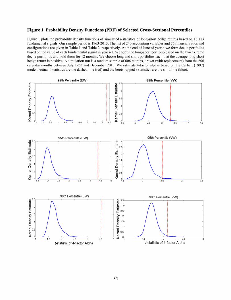
We can also illustrate our findings graphically. Figure 1 plots the probability density

distribution of the bootstrapped 99th, 95th, and 90th percentiles of 4-factor alpha t-statistics. It also

plots the actual t-statistics as a vertical line. These graphs show that the actual t-statistics are much

18

larger when compared to their bootstrapped counterparts, confirming that they are unlikely to be

driven by random chance. Moreover, the distributions of bootstrapped t-statistics are highly non-

normal. In particular, each graph exhibits a significant positive skewness. As a result, the inference

from the conventional tests under the normality assumptions can be misleading.

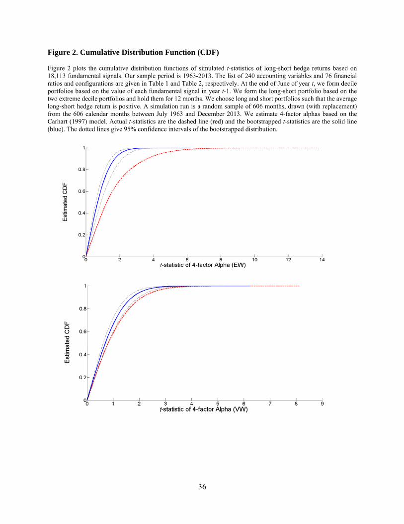
We also plot the cumulative distribution function (CDF) of t(α) estimates for both the actual

data and the simulated data. Panel A of Figure 2 shows the CDF for equal-weighted returns while

Panel B shows the CDF for value-weighted returns. In both graphs, the actual CDF is significantly

below that of the simulated data, which indicates that the right tail of the actual t-statistics is much

thicker than that of the simulated data. This result again shows that the performance of top signals

is not due to sampling variation.

3.2. Comparisons with Standard Multiple-testing Methods

In addition to the bootstrap approach, the literature has proposed several alternative tests

to address the multiple-testing issue. In this section, we implement several of these tests to examine

whether they lead to different inferences from that of the bootstrap approach. We follow HLZ

(2014) and consider the following three tests: (1) Bonferroni; (2) Holm; and (3) Benjamini,

Hochberg, and Yekutieli (BHY). Bonferroni’s adjustment for multiple testing is the simplest, in

which the original p-value is multiplied by the total number of tests. Holm’s adjustment is a

refinement of Bonferoni but involves ordering of p-values and thus depends on the entire

distribution of p-values. BHY aim to control the false discovery rate and also depends on the

distribution of p-values. For brevity, we refer the readers to HLZ for a detailed discussion of these

tests.

19

The above-mentioned multiple testing methods assume that the outcomes of all tests are

observed. In reality, however, significant factors are more likely to be published than insignificant

ones, thus creating a problem in applying these three tests. This is not an issue in our context, as

we assume all the factors tried and considered by researchers are in the universe that we

constructed. Therefore, we can easily implement the Bonferroni, Holm, and BHY tests for our

sample of fundamental signals.

Table 5 reports the results. For brevity, we report the results for 4-factor alphas only.13 In

Panel A, we consider the significance level of 5 percent. The cutoff t-values for the Bonferroni test

is 4.58 for equal-weighted returns. Based on this cutoff value, 4.33% of our 18,113 signals are

significant. The cutoff t-values for the Holm test is identical to that of the Bonferroni test.

Compared with the Bonferroni and Holm tests, the BHY test is much less stringent with a t-

statistics cutoff value of 3.24.

The cutoff t-values for value-weighted returns are similar to those for equal-weighted

returns. However, because the actual t-statistics for value-weighted returns are much lower, the

percentage of significant signals are also significantly lower. In fact, no more than 0.02% of the

signals are significant under either of Bonferroni, Holm, and BHY tests when we use value-

weighted returns. This finding is in sharp contrast to our bootstrap results. Using a bootstrap

approach, we show in Tables 3 and 4 that a large number of signals exhibit significant value-

weighted long-short performance after accounting for sampling variation. There are two reasons

for this difference. First, standard multiple-testing procedures are known to be too stringent,

especially the Bonferroni procedure, which assumes all tests are independent. Second, standard

13 The results for raw returns and 1- and 3-factor alphas are qualitatively similar.

20

tests do not take into account the exact nature and magnitude of the cross-sectional dependencies

in the data, and therefore may lead to false inferences.

Panel B presents the results for the significance level of 1 percent. As expected, the cutoff

t-values are much higher than those in Panel A. Nevertheless, a large number of fundamental

signals exhibit significant long-short performance when looking at equal-weighted returns. This

inference is similar to that of our bootstrap analysis. However, when we look at the value-weighted

returns, the percentage of significant signals is only 0.01%, 0.01%, and 0% for the Bonferroni,

Holm, and BHY tests, respectively. This finding is once again dramatically different from our

bootstrap analysis.

3.3. Sub-periods

3.3.1. Bootstrap Results

We divide our sample period into two halves of roughly equal length (1963-1987 and 1988-

2013) and examine the predictive ability of fundamental signals in both sub-periods. Table 6

presents the results. We report two primary findings. First, the predictive ability of fundamental

signals is evident in both sub-periods. All the extreme percentiles of t-statistics have a bootstrapped

p-value of 5% or lower except the 100th percentile of value-weighted returns. Second, there is no

evidence that, as a whole, the predictive ability of fundamental signals has attenuated from the first

half of our sample period to the second half. For example, the 99th percentile of t-statistics is 5.03

(3.19) for equal-weighted (value-weighted) returns during 1963-1987, and is 5.34 (3.17) during

the second half. The 95th percentiles show a similar pattern. If anything, the t-statistics are slightly

higher in the second half of the sample period.

21

3.3.2. Transition Matrix

Having examined the predictive ability of fundamental signals during each of the two sub-

periods, we next examine the persistence of the performance of individual signals. This analysis

is important because previous studies (e.g., Sullivan, Timmermann, and White (2001)) suggest

that the analysis of sub-period stability is a remedy against data mining.

To measure stability, we construct a transition matrix for the t-statistics between 1963-

1987 and 1988-2013. Specifically, we sort signals into quintiles based on their t-statistics during

each sub-period and report the percentage of signals in a given quintile during the first half of the

sample period moved to a particular quintile in the second half. If the predictive ability of

fundamental signals is due to chance, then we should expect all numbers in the transition matrix

to be around 20%. On the other hand, if the predictive ability is real and stable, then we should

expect the diagonal terms of the transition matrix (particularly the two corners) to be significantly

greater than 20%. In this analysis, we do not take the absolute value of the t-statistics (e.g., the

sign of the t-statistics for the asset growth anomaly stays negative), as changing from an extreme

positive t-statistics to an extreme negative t-statistics or vice versa should be interpreted as unstable

rather than stable.

Panel A of Table 7 reports the results. Focusing on equal-weighted returns in the left panel,

we find strong evidence of cross-period stability. More than 50% of the signals ranked in the

bottom quintile during the first half of the sample period continue to be ranked in the bottom

quintile during the second half, while less than 8% of these signals move to the top quintile.

Similarly, more than 30% of the signals ranked in the top quintile continue to stay in the same

quintile during the second half of the sample period, while only 3.1% of the signals switch to the

22

bottom quintile. Unreported tests indicate that these percentages are significantly different from

20% (the unconditional average). The results for value-weighted returns are qualitatively similar.

3.3.3. Performance Persistence

Another way to evaluate whether the predictive ability of fundamental signals is stable is

to look at the performance persistence of fundamental-based trading strategies. This is a common

approach in the mutual fund and hedge fund literature to separate skill from luck. As in our

previous analysis, we divide our sample period into two halves. We estimate the alpha for each

signal during the first half of our sample period. We then sort all signals into decile portfolios

based on the t-statistics of the estimated alpha. We form equal-weighted portfolios of these

anomalies and hold the portfolios during the second half of our sample period. We report the

performance of the two extreme deciles as well as their difference in Panel B of Table 7. As in the

previous section, we do not take the absolute value of either alphas or t-statistics.

We find strong evidence of performance persistence. Looking at the equal-weighted raw

returns, we find that those signals ranked in the bottom decile (D1) during the first half of our

sample period continue to exhibit a negative and significant long-short return of -0.43% per month

during the second half. In contrast, those signals ranked in the top decile (D10) during the first half

of our sample period exhibit a positive and significant long-short return of 0.17% per month during

the second half. The difference between D10 and D1 is 0.6% per month and highly statistically

significant. The result is robust whether we use 1-, 3-, or 4-factor alphas and whether we examine

equal-weighted or value-weighted long-short returns. The difference between D10 and D1 is

economically meaningful and statistically significant across all specifications.

Overall, our analysis of the performance of fundamental-based trading rules across sub-

periods provides further evidence that the predictive ability of fundamental signals is unlikely to

23

be driven by data mining. It also suggests that investors could have adopted a recursive decision

rule to identify the best performing signals and have used this information to produce genuinely

superior out-of-sample performance.

3.4. Evidence on Behavioral Explanations

We have shown that the observed performance of top-ranked signals is unlikely to be a

result of data mining. In this section, we investigate whether fundamental-based anomalies are

consistent with mispricing-based explanations. In particular, we hypothesize that financial

statement variables contain valuable information about future firm performance, but the market

fails to incorporate this information into stock prices in a timely manner. We perform three tests.

We first examine long-short returns by firm characteristics. We then investigate the relation

between long-short returns and investor sentiment. Finally, we measure the extent to which the

long-short returns of fundamental-based strategies are concentrated around earnings

announcement periods.

3.4.1. By Firm Characteristics

In this section, we partition our sample by size, idiosyncratic volatility, institutional

ownership, and analyst coverage and then repeat our analysis for each sub-group of stocks. Our

analysis has two specific objectives. First, we want to examine if our main results are robust across

all sub-samples of stocks, e.g., small and large stocks. This analysis is important because if the

results only hold for small stocks and not for large stocks, then the economic significance of our

results will be limited. Second, behavioral arguments suggest that if anomaly returns are due to

mispricing, then the predictability should be more pronounced among stocks that are more costly

24

to trade, held by unsophisticated investors, have larger arbitrage risk, and covered by fewer

analysts. Our second objective is to test this prediction.

We perform double sorts. We divide our sample stocks into two portfolios by each firm

characteristic, and then independently sort the sample into deciles based on each fundamental

signal. We conduct our bootstrap analysis for each sub-group of stocks. For each firm

characteristic, we also test for the difference in the cross-sectional percentile of t-statistics between

the two sub-groups of stocks, e.g., small versus large stocks.

Panel A of Table 8 presents the results for firm size. Small stocks typically have higher

transactions costs, greater information asymmetry, and more limited arbitrage. If the abnormal

returns to fundamental-based trading strategies represent mispricing, then we would expect the

predictive ability to be stronger among small stocks. We find evidence consistent with this

prediction. For example, the 99th percentile of t-statistics for equal-weighted returns is 6.22 for

small stocks, and only 3.18 for large stocks. The difference of 3.04 in t-statistics is highly

statistically significant.14 Similarly, the 95th percentile of t-statistics is 4.42 for small stocks and

2.39 for large stocks, and the difference of 2.03 is also statistically significant. These results

suggest that the predictive ability of fundamental signals is significantly stronger among small

stocks. In spite of the large difference between small and large stocks, our main results hold for

both small and large stocks. In particular, the bootstrapped p-values associated with extreme

percentiles are uniformly zero for small stocks and less than 5% for large stocks except for the

100th percentile. The value-weighted results presented in the right panel paint a similar picture.

Overall, our main finding is robust across small and large stocks, and more importantly, the

predictive ability of top-ranked fundamental signals is more pronounced among small stocks.

14 We test for the difference between small and large stocks by using the standard deviation of the difference in 1,000 simulations as the standard error.

25

Panel B reports the results for idiosyncratic volatility (IVOL). Previous literature (e.g.,

Shleifer and Vishny (1997) and Pontiff (2006)) suggest that IVOL is a primary limit to arbitrage.

To the extent that the predictive power of fundamental signals reflect market inefficiency, we

expect the results to be more pronounced among high-IVOL stocks. Results in Panel B reveal

strong evidence that the t-statistics for equal-weighted returns are significantly higher among high-

IVOL stocks than low-IVOL stocks. For example, the 95th percentile of t-statistics is 4.44 for high-

IVOL stocks and only 3.14 for low-IVOL stocks. The difference is statistically significant. For

value-weighted returns, the t-statistics are higher for high-IVOL stocks, but the difference is

insignificant.15

Panel C presents the results for institutional ownership (IO). Institutional investors are

more sophisticated and better informed than individual investors. To the extent that the predictive

ability of financial statement variables represent misreaction to public information by uninformed

investors, we would expect this predictability to be stronger among low-institutional ownership

stocks. Our results confirm this conjecture. For equal-weighed returns, we find large and

statistically significant differences in t-statistics between high- and low-IO stocks. For example,

the 99th percentile of t-statistics is 6.07 for low-IO stocks and 3.82 for high-IO stocks. The value-

weighted results are lower in magnitudes but qualitatively similar.

In our final firm characteristic analysis, we focus on analyst coverage. Financial analysts

play an important role in interpreting and disseminating financial information. If the predictive

ability of fundamental signals is due to market failing to fully incorporate public financial

statement information, we would expect this predictability to be attenuated among stocks with

15 There are two reasons for the lack of significant difference when we use value-weighted returns. First, large stocks carry more weights in value-weighted returns and the marginal impact of IVOL is smaller among large stocks. Second, due to data constraints we only partition our sample into two portfolios based on IVOL, which makes it difficult to find a significant difference between high- and low-IVOL stocks.

26

more extensive analyst coverage. Results contained in Panel D of Table 8 lend support to this

prediction. We find statistically significant difference in t-statistics between low- and high-analyst

coverage stocks, whether we examine equal-weighted returns or value-weighted returns.16

Overall, our main findings hold for all sub-groups of stocks, suggesting they are not solely

attributed to small, neglected stocks, which comprise only a small percentage of the entire stock

market based on market capitalization. Consistent with behavioral explanations, we find that the

predictive ability of fundamental signals are stronger among small stocks and stocks with higher

idiosyncratic volatility, lower institutional ownership, and fewer analysts.

3.4.2. Investor Sentiment

To the extent that stock return anomalies are driven by mispricing, overpricing should be

more prevalent than underpricing because shorting is more costly. As a consequence, anomaly

returns should be significantly higher following high-sentiment periods than low sentiment periods

(Stambaugh, Yuan, and Yu (2012)). Examining thirteen well-documented anomalies, Stambaugh,

Yuan, and Yu find evidence consistent with this prediction.

We test the above prediction using our sample of fundamental signals. We obtain the

investor sentiment index of Baker and Wurgler (2006) from Jeffrey Wurgler’s website. Following

Stambaugh, Yuan, and Yu (2012), we divide our sample into high- and low-sentiment periods

based on the median sentiment index level. We then compute anomaly returns separately for the

periods following high and low sentiment levels. We perform this analysis for the top 10, 5, and 1

percent of fundamental signals (ranked based on the t-statistics of 4-factor alphas).

16 IVOL, IO, and the number of analysts are correlated with size. As such, the cross-sectional impact of IVOL, IO, and analyst coverage may simply be a manifestation of the effect of size. To mitigate this concern, we perform a triple sort, and repeat our analysis by using size-stratified IVOL, IO, and analyst coverage. We find that our results are similar in this alternative test, suggesting that IVOL, IO, and analyst coverage has an incremental impact on fundamental-based anomalies.

27

Table 9 presents the results. We find that the long-short returns of top-ranked fundamental

signals are significantly higher following high-sentiment periods than following low-sentiment

periods. For example, the average long-short return for the top 10 percent signals is 0.56% per

month following high-sentiment periods, and 0.36% per month following low-sentiment period.

The difference of 0.2% is statistically significant with a t-statistics of 3.15. The results for the top

5% and 1% signals are qualitatively similar and quantitatively higher. The difference in long-short

returns is 0.22% and 0.26% for the top 5% and top 1% of signals, respectively, both statistically

significant. The value-weighted results are more pronounced than equal-weighted results. For

example, the average anomaly return among the top 1% signals is 0.88% per month following

high-sentiment periods, and only 0.35% per month following low-sentiment periods. The

difference of 0.53% per month economically and statistically significant. Overall, our finding

strongly supports the mispricing-based explanations.

3.4.3. Earnings Announcements

Next, we investigate the extent to which the long-short returns of top signals are

concentrated around subsequent earnings announcements. This test follows La Porta et al. (1997)

and Bernard, Thomas, and Wahlen (1997) and is based on the following argument. According to

mispricing-based explanations of anomalies, predictable stock returns arise from corrections of

mispricing. If a stock is mispriced, then price corrections will more likely occur around subsequent

information releases when investors update their prior beliefs. Earnings information is arguably

the most important piece of information for publicly traded firms; therefore, a disproportionate

amount of abnormal returns should occur around future earnings announcements.

We compute earnings announcement return (EAR) during the three-day periods around

each announcement date. We then sum up the EAR over the subsequent four quarterly

28

announcements for each firm. For each fundamental signal in our sample, we compute the average

EAR separately for firms in the long and short portfolios and then compute the difference in EAR

between the long and short portfolios. Table 10 reports the results. For comparison, we also report

the total long-short return over the entire 12-month holding period. As in the previous analysis, we

focus on the top 1, 5, and 10 percent of signals sorted on 4-factor alpha t-statistics.

Looking at equal-weighted returns, we find that the average EAR is statistically significant.

Moreover, the EAR represents about 18% of the total long-short hedge returns. For example,

among the top 1% signals ranked by four-factor alpha t-statistics, the average total long-short

return is 8.55% per year. The average difference in EAR between long and short portfolios is

1.54% during the four quarterly earnings announcement periods. Since earnings announcement

periods comprise less than 5% of total number of trading days (12 out of 252), the above result

suggests that the long-short return is almost three times higher during earnings announcement

periods when compared to non-announcement periods.17 The value-weighted results show a lower

percentage (12-13%) of total long-short return accrued during earnings announcement periods.

Nonetheless, we still find that the long-short returns are significantly higher during earnings

announcements periods than other periods. Overall, our evidence is consistent with behavioral

explanations and suggests that fundamental-based anomalies at least partly result from investor

expectation errors.

3.5. Robustness Tests

We have already shown that our main findings are robust to alternative portfolio weighting

schemes and alternative risk-adjustment models, and they hold in both halves of our sample period

17 These percentages are likely understated because of the post-earnings-announcement drift.

29

and among sub-groups of stocks sorted by various firm characteristics. In this section, we perform

a number of additional robustness tests to further ensure that our results are not sensitive to our

methodological choices.

3.5.1. Bootstrap Alphas

In this section, we apply the bootstrap procedure to alphas instead of t-statistics. Recall that

we focus on t-statistics in our main analysis because t-statistics has better sampling properties. In

particular, t-statistics is less prone to the extreme outlier problem. Nevertheless, it is informative

to examine the magnitude of the abnormal performance by looking at alphas. Table 11 summarizes

the results. The structure of this table is identical to that of Tables 3 and 4 except that the numbers

reported in Table 11 are alphas rather than t-statistics. The results show that the extreme deciles

of alphas are large and not attributable to sampling variation. For example, the 99th percentile of

equal-weighted 1-factor alphas is 1.1% per month and this number is greater than its counterparts

in all but 1.2% of the simulation runs. The maximum alpha, i.e., the 100th percentile is generally

insignificant in part because of the outlier problem. However, the other extreme percentiles are

generally significant. Overall, despite the relatively poor sampling properties of alpha estimates,

we find evidence that the extreme alphas of the best performing signals are not due to sampling

variation.

3.5.2. Industry-adjusted Ratios

One might argue that financial ratios are industry specific, so it may be more meaningful

to compare a company’s financial ratios to its industry peers. In an untabulated robustness test, we

subtract the industry median from each firm’s fundamental signal before forming portfolios. We

find essentially the same results when we use industry-adjusted ratios. In some cases, the results

are slightly better, confirming that industry-adjustment does provide incremental information.

30

3.5.3. Alternative Universe of Signals

A key innovation of our paper is to construct a universe of fundamental signals using

permutational arguments. In doing so, we have to make choices on the list of accounting variables

and financial ratios. To ensure robustness of our findings, we repeat our analyses on several

alternative universe of fundamental signals. In particular, we find that our results are qualitatively

identical when we impose more (or less) stringent data requirements on the accounting variables

(e.g., require a minimum of 2,000 average observations per year as opposed to 1,000). We also

find that our results are not driven by any specific base variables or specific signals we use. For

example, our results are qualitatively identical when we consider only those signals that are scaled

by total assets or total sales. These results are not tabulated in the paper but are available upon

request.

3.5.4. Number of Simulation Runs

Throughout the paper, we perform 1,000 simulations in our bootstrap analysis. To gauge

robustness, we increase the number of simulation runs to 10,000 and repeat our main analysis in

Table 4. We perform this robustness test only for Table 4 because of high computational cost.

Untabulated results indicate that the results in Table 4 are essentially unchanged when we use

10,000 simulations. Moreover, the results hold for each of the ten 1,000-simulation subsets.

4. Conclusions

Previous studies have documented hundreds of cross-sectional return anomalies. These

findings have largely been considered without accounting for the extensive search preceding them.

In this paper, we evaluate the data-mining bias in cross-sectional return anomalies by examining

an important class of anomaly variables, i.e., fundamental signals derived from financial

31

statements, and by using a bootstrap approach. We use permutational arguments to construct a

“universe” of over 18,000 fundamental signals from financial statements. We find that a large

number of fundamental signals are significant predictors of cross-sectional stock returns even after

accounting for data mining. This predictive ability is more pronounced among small, low-

institutional ownership, low-analyst coverage, and high-idiosyncratic volatility stocks, providing

support for the behavioral explanations of fundamental-based anomalies. We also find that the

long-short returns associated with fundamental signals are disproportionately concentrated around

subsequent earnings announcements and are significantly higher following high-sentiment

periods. This evidence suggests that fundamental-based anomalies are more likely to result from

mispricing and expectation errors. The long-short returns of the best performing signals exhibit

strong persistence across sub-periods, providing further evidence against data mining. Our

evidence suggests that fundamental-based anomalies are not a product of data mining and they are

more likely to reflect mispricing. Although we focus only on financial statement variables in this

paper, our approach is general and can be applied to other categories of anomaly variables such as

macroeconomic variables.

32

References Abarbanell, J.S., and B.J. Bushee, 1998, Abnormal returns to a fundamental analysis strategy, Accounting Review 73, 19-45. Baker, M., and J. Wurgler, 2006, Investor sentiment and the cross-section of stock returns, Journal of Finance 61, 1645-1680. Bernard, V., J. Thomas, and J. Wahlen, 1997, Accounting-based stock price anomalies: Separating market inefficiencies from risk, Contemporary Accounting Research 14, 89-136. Carhart, M., 1997, On persistence in mutual fund performance, Journal of Finance 52, 57-82. Chan, K., L. Chan, N. Jegadeesh, and L. Lakonishok, 2006, Earnings quality and stock returns, Journal of Business 79, 1041-1082. Cooper, M., H. Gulen, and M. Schill, 2008, Asset growth and the cross-section of stock returns, Journal of Finance 63, 1609-1651. Eisfeldt, A.L., D. Papanikolaou, 2013, Organization capital and the cross-section of expected returns. Journal of Finance 68, 1365-1406. Fama, Eugene F. and Kenneth R. French, 1996. Multifactor explanations of asset pricing anomalies, The Journal of Finance 51, 55-84. Fama, E., and K. French, 2008, Dissecting anomalies, Journal of Finance 63, 1653-1678. Fama, E., K. French, 2010, Luck versus skill in the cross section of mutual fund returns, Journal of Finance 65, 1915-1947. Foster, F. Douglas, Tom Smith and Robert E. Whaley, 1997, Assessing goodness-of-fit of asset pricing models: the distribution of the maximal R2, Journal of Finance 52, 591-607. Green, J., J. Hand, and X. Zhang, 2013, The supraview of return predictive signals, Review of Accounting Studies 18, 692-730. Green, Jeremiah, John RM Hand and X. Frank Zhang, 2013, The remarkable multidimensionality in the cross section of expected US stock returns, Working Paper, Pennsylvania State University. Harvey, C., Y. Liu, and H. Zhu, 2014, … and the cross-section of stock returns, Working paper, Duke University. Jegadeesh, Narasimhan and Sheridan Titman, 2001. Profitability of momentum strategies: An evaluation of alternative explanations, Journal of Finance 56, 699-720. Kogan, L., and M. Tian, 2013, Firm characteristics and empirical factor models: A data-mining

33

experiment, Working paper, MIT. Kosowski, Robert, Allan Timmermann, Russ Wermers and Hal White, 2006, Can mutual fund “stars” really pick stocks? New evidence from a Bootstrap analysis, Journal of Finance 61, 2551- 2595. La Porta, J. Lakonishok, A. Shleifer, and R. Vishny, 1997, Good news for value stocks: Further evidence on market efficiency, Journal of Finance 52, 859-874. Lev, B., and S.R. Thiagarajan, 1993. Fundamental information analysis, Journal of Accounting Research 31, 190-215. Lo, Andrew and Craig Mackinlay, 1990, Data-snooping biases in tests of financial asset pricing models, Review of financial studies 3, 431-467. McLean, R., and J. Pontiff, 2014, Does academic research destroy stock return predictability? Forthcoming Journal of Finance. Merton, R., 1987, On the state of the efficient market hypothesis in financial economics, Macroeconomics and Finance: Essays in Honor of Franco Modigliani, MIT Press, 93-124. Novy-Marx, R, 2013, The other side of value: The gross profitability premium, Journal of Financial Economics 108, 1-28. Ou, Jane A. and Stephen H. Penman, 1989, Financial statement analysis and the prediction of stock returns, Journal of Accounting & Economics 11, 295-329. Piotroski, Joseph D., 2000, Value investing: The use of historical financial statement information to separate winners from losers, Journal of Accounting Research 38, 1-41. Pontiff, J., 2006, Costly arbitrage and the myth of idiosyncratic risk, Journal of Accounting and Economics 42, 35-52. Shleifer, Andrei and Robert W. Vishny, 1997. The limits of arbitrage, Journal of Finance 52, 35-55. Stambaugh, R., J. Yu, and Y. Yuan, 2012, The short of it: Investor sentiment and anomalies, Journal of Financial Economics 104, 288-302. Sullivan, Ryan, Allan Timmermann and Halbert White, 1999, Data-snooping, technical trading rule performance, and the bootstrap, Journal of Finance 54, 1647-1691. Sullivan, Ryan, Allan Timmermann and Halbert White, 2001, Dangers of data mining: The case of calendar effects in stock returns, Journal of Econometrics 105, 249-286.

34

Thomas, J., and H. Zhang, 2002, Inventory changes and future returns, Review and Accounting Studies 7, 163-187. Treynor, J., and F. Black, 1973, How to use security analysis to improve portfolio selection, Journal of Business 46, 66-86. White, Halbert, 2000, A reality check for data snooping, Econometrica 68, 1097-1126.

35

Figure 1. Probability Density Functions (PDF) of Selected Cross-Sectional Percentiles Figure 1 plots the probability density functions of simulated t-statistics of long-short hedge returns based on 18,113 fundamental signals. Our sample period is 1963-2013. The list of 240 accounting variables and 76 financial ratios and configurations are given in Table 1 and Table 2, respectively. At the end of June of year t, we form decile portfolios based on the value of each fundamental signal in year t-1. We form the long-short portfolio based on the two extreme decile portfolios and hold them for 12 months. We choose long and short portfolios such that the average long-short hedge return is positive. A simulation run is a random sample of 606 months, drawn (with replacement) from the 606 calendar months between July 1963 and December 2013. We estimate 4-factor alphas based on the Carhart (1997) model. Actual t-statistics are the dashed line (red) and the bootstrapped t-statistics are the solid line (blue).

36

Figure 2. Cumulative Distribution Function (CDF) Figure 2 plots the cumulative distribution functions of simulated t-statistics of long-short hedge returns based on 18,113 fundamental signals. Our sample period is 1963-2013. The list of 240 accounting variables and 76 financial ratios and configurations are given in Table 1 and Table 2, respectively. At the end of June of year t, we form decile portfolios based on the value of each fundamental signal in year t-1. We form the long-short portfolio based on the two extreme decile portfolios and hold them for 12 months. We choose long and short portfolios such that the average long-short hedge return is positive. A simulation run is a random sample of 606 months, drawn (with replacement) from the 606 calendar months between July 1963 and December 2013. We estimate 4-factor alphas based on the Carhart (1997) model. Actual t-statistics are the dashed line (red) and the bootstrapped t-statistics are the solid line (blue). The dotted lines give 95% confidence intervals of the bootstrapped distribution.

37

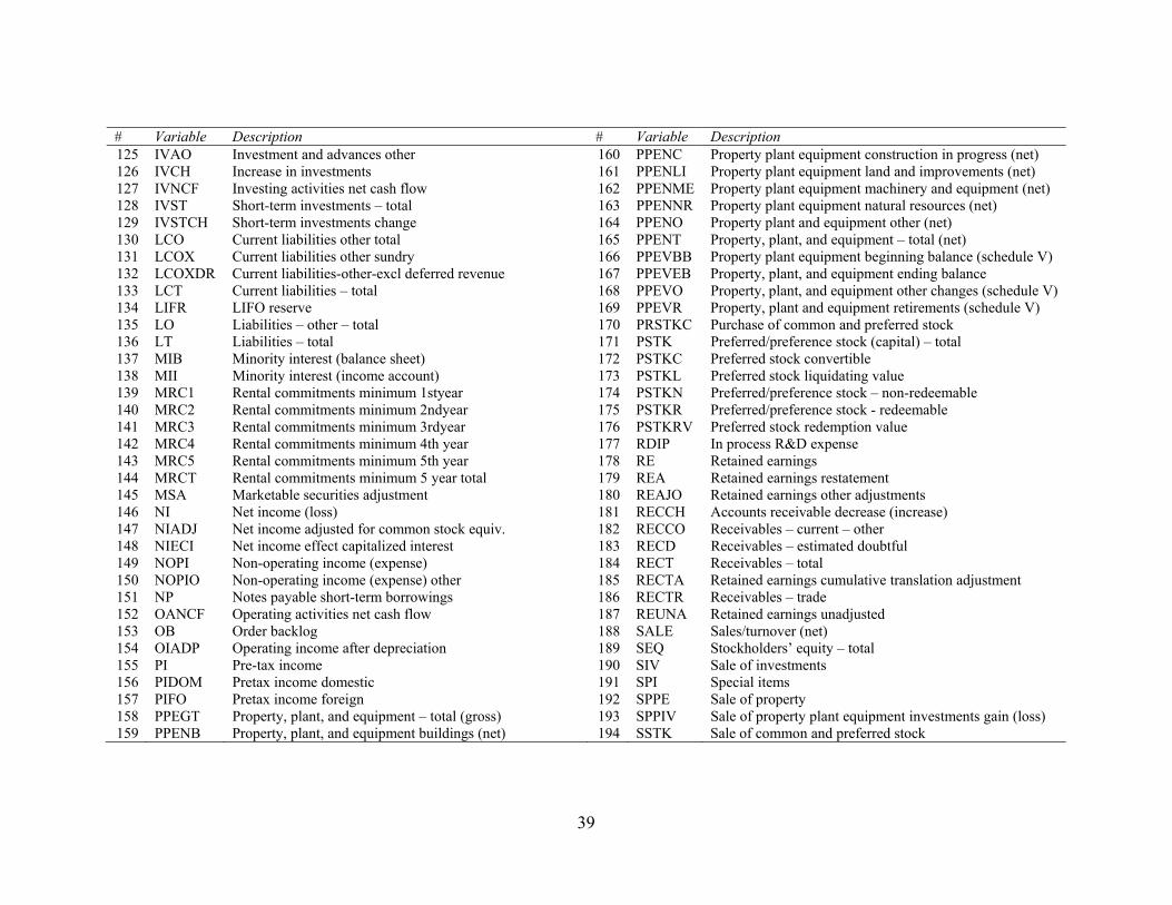
Table 1 List of Accounting Variables Table 1 lists the 240 accounting variables used in this study and their descriptions. Our sample period is 1963-2013. We begin with all accounting variables on the balance sheet, income statement, and cash flow statement included in the annual Compustat database. We exclude all variables with fewer than 20 years of data or fewer than 1,000 firms with non-missing data on average per year. We exclude per-share based variables such as book value per share and earnings per share. We remove LSE (total liabilities and equity), REVT (total revenue), OIBDP (operating income before depreciation), XDP (depreciation expense) because they are identical to TA (total assets), SALE (total sale), EBITDA (earnings before interest) and DFXA (depreciation of tangible fixed assets) respectively.

# Variable Description # Variable Description 1 ACCHG Accounting changes–cumulative effect 29 COGS Cost of goods sold 2 ACO Current assets other total 30 CSTK Common/ordinary stock (capital) 3 ACOX Current assets other sundry 31 CSTKCV Common stock-carrying value 4 ACT Current assets- total 32 CSTKE Common stock equivalents – dollar savings 5 AM Amortization of intangibles 33 DC Deferred charges 6 AO Assets – other 34 DCLO Debt capitalized lease obligations 7 AOLOCH Assets and liabilities other net change 35 DCOM Deferred compensation 8 AOX Assets – other - sundry 36 DCPSTK Convertible debt and stock 9 AP Accounts payable – trade 37 DCVSR Debt senior convertible 10 APALCH Accounts payable & accrued liabilities increase/decrease 38 DCVSUB Debt subordinated convertible 11 AQC Acquisitions 39 DCVT Debt – convertible 12 AQI Acquisitions income contribution 40 DD Debt debentures 13 AQS Acquisitions sales contribution 41 DD1 Long-term debt due in one year 14 AT Assets – total 42 DD2 Debt Due in 2nd Year 15 BAST Average short-term borrowing 43 DD3 Debt Due in 3rd Year 16 CAPS Capital surplus/Share premium reserve 44 DD4 Debt Due in 4th Year 17 CAPX Capital expenditure 45 DD5 Debt Due in 5th Year 18 CAPXV Capital expenditure PPE Schedule V 46 DFS Debt finance subsidiary 19 CEQ Common/ordinary equity - total 47 DFXA Depreciation of tangible fixed assets 20 CEQL Common equity liquidation value 48 DILADJ Dilution adjustment 21 CEQT Common equity tangible 49 DILAVX Dilution available excluding extraordinary items 22 CH Cash 50 DLC Debt in current liabilities - total 23 CHE Cash and short-term investments 51 DLCCH Current debt changes 24 CHECH Cash and cash equivalents increase/(decrease) 52 DLTIS Long-term debt issuance 25 CLD2 Capitalized leases - due in 2nd year 53 DLTO Other long-term debt 26 CLD3 Capitalized leases - due in 3rdyear 54 DLTP Long-term debt tied to prime 27 CLD4 Capitalized leases - due in 4thyear 55 DLTR Long-term debt reduction 28 CLD5 Capitalized leases - due in 5thyear 56 DLTT Long-term debt - total

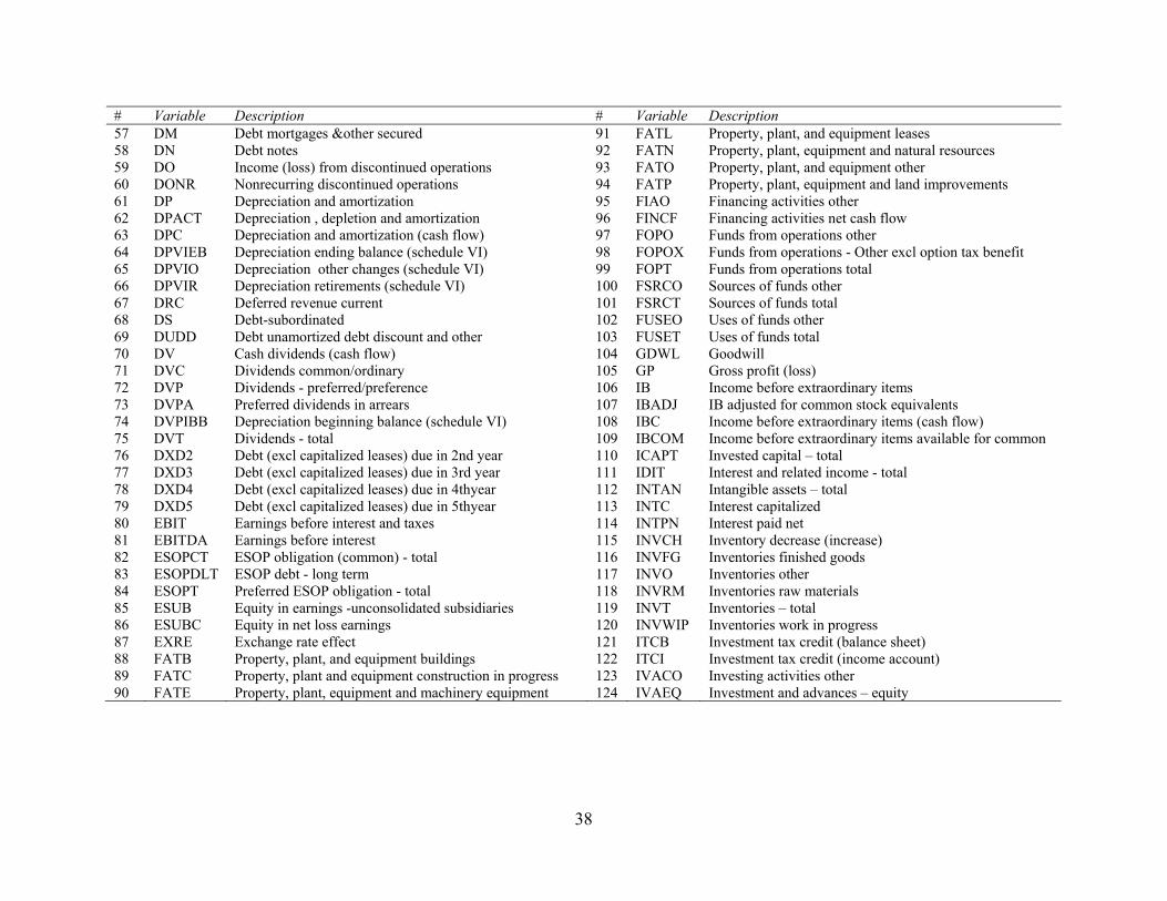
38

# Variable Description # Variable Description 57 DM Debt mortgages &other secured 91 FATL Property, plant, and equipment leases 58 DN Debt notes 92 FATN Property, plant, equipment and natural resources 59 DO Income (loss) from discontinued operations 93 FATO Property, plant, and equipment other 60 DONR Nonrecurring discontinued operations 94 FATP Property, plant, equipment and land improvements 61 DP Depreciation and amortization 95 FIAO Financing activities other 62 DPACT Depreciation , depletion and amortization 96 FINCF Financing activities net cash flow 63 DPC Depreciation and amortization (cash flow) 97 FOPO Funds from operations other 64 DPVIEB Depreciation ending balance (schedule VI) 98 FOPOX Funds from operations - Other excl option tax benefit 65 DPVIO Depreciation other changes (schedule VI) 99 FOPT Funds from operations total 66 DPVIR Depreciation retirements (schedule VI) 100 FSRCO Sources of funds other 67 DRC Deferred revenue current 101 FSRCT Sources of funds total 68 DS Debt-subordinated 102 FUSEO Uses of funds other 69 DUDD Debt unamortized debt discount and other 103 FUSET Uses of funds total 70 DV Cash dividends (cash flow) 104 GDWL Goodwill 71 DVC Dividends common/ordinary 105 GP Gross profit (loss) 72 DVP Dividends - preferred/preference 106 IB Income before extraordinary items 73 DVPA Preferred dividends in arrears 107 IBADJ IB adjusted for common stock equivalents 74 DVPIBB Depreciation beginning balance (schedule VI) 108 IBC Income before extraordinary items (cash flow) 75 DVT Dividends - total 109 IBCOM Income before extraordinary items available for common 76 DXD2 Debt (excl capitalized leases) due in 2nd year 110 ICAPT Invested capital – total 77 DXD3 Debt (excl capitalized leases) due in 3rd year 111 IDIT Interest and related income - total 78 DXD4 Debt (excl capitalized leases) due in 4thyear 112 INTAN Intangible assets – total 79 DXD5 Debt (excl capitalized leases) due in 5thyear 113 INTC Interest capitalized 80 EBIT Earnings before interest and taxes 114 INTPN Interest paid net 81 EBITDA Earnings before interest 115 INVCH Inventory decrease (increase) 82 ESOPCT ESOP obligation (common) - total 116 INVFG Inventories finished goods 83 ESOPDLT ESOP debt - long term 117 INVO Inventories other 84 ESOPT Preferred ESOP obligation - total 118 INVRM Inventories raw materials 85 ESUB Equity in earnings -unconsolidated subsidiaries 119 INVT Inventories – total 86 ESUBC Equity in net loss earnings 120 INVWIP Inventories work in progress 87 EXRE Exchange rate effect 121 ITCB Investment tax credit (balance sheet) 88 FATB Property, plant, and equipment buildings 122 ITCI Investment tax credit (income account) 89 FATC Property, plant and equipment construction in progress 123 IVACO Investing activities other 90 FATE Property, plant, equipment and machinery equipment 124 IVAEQ Investment and advances – equity

39

# Variable Description # Variable Description 125 IVAO Investment and advances other 160 PPENC Property plant equipment construction in progress (net) 126 IVCH Increase in investments 161 PPENLI Property plant equipment land and improvements (net) 127 IVNCF Investing activities net cash flow 162 PPENME Property plant equipment machinery and equipment (net) 128 IVST Short-term investments – total 163 PPENNR Property plant equipment natural resources (net) 129 IVSTCH Short-term investments change 164 PPENO Property plant and equipment other (net) 130 LCO Current liabilities other total 165 PPENT Property, plant, and equipment – total (net) 131 LCOX Current liabilities other sundry 166 PPEVBB Property plant equipment beginning balance (schedule V) 132 LCOXDR Current liabilities-other-excl deferred revenue 167 PPEVEB Property, plant, and equipment ending balance 133 LCT Current liabilities – total 168 PPEVO Property, plant, and equipment other changes (schedule V) 134 LIFR LIFO reserve 169 PPEVR Property, plant and equipment retirements (schedule V) 135 LO Liabilities – other – total 170 PRSTKC Purchase of common and preferred stock 136 LT Liabilities – total 171 PSTK Preferred/preference stock (capital) – total 137 MIB Minority interest (balance sheet) 172 PSTKC Preferred stock convertible 138 MII Minority interest (income account) 173 PSTKL Preferred stock liquidating value 139 MRC1 Rental commitments minimum 1styear 174 PSTKN Preferred/preference stock – non-redeemable 140 MRC2 Rental commitments minimum 2ndyear 175 PSTKR Preferred/preference stock - redeemable 141 MRC3 Rental commitments minimum 3rdyear 176 PSTKRV Preferred stock redemption value 142 MRC4 Rental commitments minimum 4th year 177 RDIP In process R&D expense 143 MRC5 Rental commitments minimum 5th year 178 RE Retained earnings 144 MRCT Rental commitments minimum 5 year total 179 REA Retained earnings restatement 145 MSA Marketable securities adjustment 180 REAJO Retained earnings other adjustments 146 NI Net income (loss) 181 RECCH Accounts receivable decrease (increase) 147 NIADJ Net income adjusted for common stock equiv. 182 RECCO Receivables – current – other 148 NIECI Net income effect capitalized interest 183 RECD Receivables – estimated doubtful 149 NOPI Non-operating income (expense) 184 RECT Receivables – total 150 NOPIO Non-operating income (expense) other 185 RECTA Retained earnings cumulative translation adjustment 151 NP Notes payable short-term borrowings 186 RECTR Receivables – trade 152 OANCF Operating activities net cash flow 187 REUNA Retained earnings unadjusted 153 OB Order backlog 188 SALE Sales/turnover (net) 154 OIADP Operating income after depreciation 189 SEQ Stockholders’ equity – total 155 PI Pre-tax income 190 SIV Sale of investments 156 PIDOM Pretax income domestic 191 SPI Special items 157 PIFO Pretax income foreign 192 SPPE Sale of property 158 PPEGT Property, plant, and equipment – total (gross) 193 SPPIV Sale of property plant equipment investments gain (loss) 159 PPENB Property, plant, and equipment buildings (net) 194 SSTK Sale of common and preferred stock

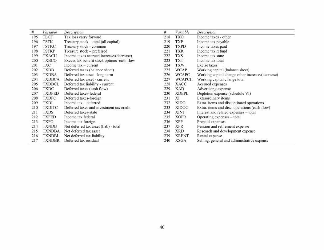
40

# Variable Description # Variable Description 195 TLCF Tax loss carry forward 218 TXO Income taxes - other 196 TSTK Treasury stock – total (all capital) 219 TXP Income tax payable 197 TSTKC Treasury stock - common 220 TXPD Income taxes paid 198 TSTKP Treasure stock – preferred 221 TXR Income tax refund 199 TXACH Income taxes accrued increase/(decrease) 222 TXS Income tax state 200 TXBCO Excess tax benefit stock options -cash flow 223 TXT Income tax total 201 TXC Income tax – current 224 TXW Excise taxes 202 TXDB Deferred taxes (balance sheet) 225 WCAP Working capital (balance sheet) 203 TXDBA Deferred tax asset - long term 226 WCAPC Working capital change other increase/(decrease) 204 TXDBCA Deferred tax asset - current 227 WCAPCH Working capital change total 205 TXDBCL Deferred tax liability - current 228 XACC Accrued expenses 206 TXDC Deferred taxes (cash flow) 229 XAD Advertising expense 207 TXDFED Deferred taxes-federal 230 XDEPL Depletion expense (schedule VI) 208 TXDFO Deferred taxes-foreign 231 XI Extraordinary items 209 TXDI Income tax – deferred 232 XIDO Extra. items and discontinued operations 210 TXDITC Deferred taxes and investment tax credit 233 XIDOC Extra. items and disc. operations (cash flow) 211 TXDS Deferred taxes-state 234 XINT Interest and related expenses – total 212 TXFED Income tax federal 235 XOPR Operating expenses – total 213 TXFO Income tax foreign 236 XPP Prepaid expenses 214 TXNDB Net deferred tax asset (liab) - total 237 XPR Pension and retirement expense 215 TXNDBA Net deferred tax asset 238 XRD Research and development expense 216 TXNDBL Net deferred tax liability 239 XRENT Rental expense 217 TXNDBR Deferred tax residual 240 XSGA Selling, general and administrative expense

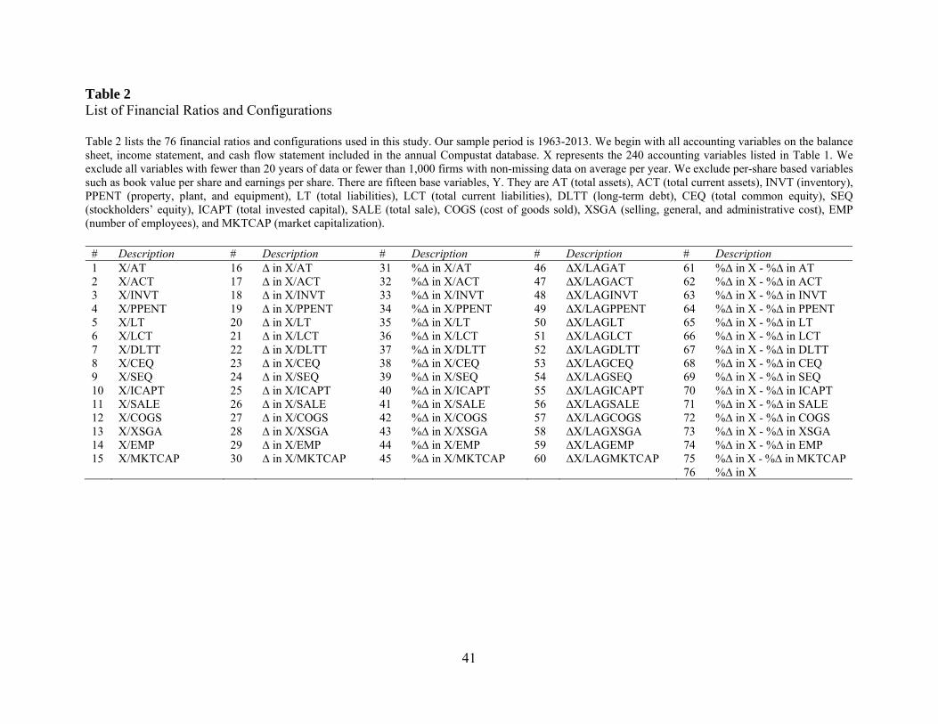
41

Table 2 List of Financial Ratios and Configurations Table 2 lists the 76 financial ratios and configurations used in this study. Our sample period is 1963-2013. We begin with all accounting variables on the balance sheet, income statement, and cash flow statement included in the annual Compustat database. X represents the 240 accounting variables listed in Table 1. We exclude all variables with fewer than 20 years of data or fewer than 1,000 firms with non-missing data on average per year. We exclude per-share based variables such as book value per share and earnings per share. There are fifteen base variables, Y. They are AT (total assets), ACT (total current assets), INVT (inventory), PPENT (property, plant, and equipment), LT (total liabilities), LCT (total current liabilities), DLTT (long-term debt), CEQ (total common equity), SEQ (stockholders’ equity), ICAPT (total invested capital), SALE (total sale), COGS (cost of goods sold), XSGA (selling, general, and administrative cost), EMP (number of employees), and MKTCAP (market capitalization).

# Description # Description # Description # Description # Description 1 X/AT 16 ∆ in X/AT 31 %∆ in X/AT 46 ∆X/LAGAT 61 %∆ in X - %∆ in AT 2 X/ACT 17 ∆ in X/ACT 32 %∆ in X/ACT 47 ∆X/LAGACT 62 %∆ in X - %∆ in ACT 3 X/INVT 18 ∆ in X/INVT 33 %∆ in X/INVT 48 ∆X/LAGINVT 63 %∆ in X - %∆ in INVT 4 X/PPENT 19 ∆ in X/PPENT 34 %∆ in X/PPENT 49 ∆X/LAGPPENT 64 %∆ in X - %∆ in PPENT 5 X/LT 20 ∆ in X/LT 35 %∆ in X/LT 50 ∆X/LAGLT 65 %∆ in X - %∆ in LT 6 X/LCT 21 ∆ in X/LCT 36 %∆ in X/LCT 51 ∆X/LAGLCT 66 %∆ in X - %∆ in LCT 7 X/DLTT 22 ∆ in X/DLTT 37 %∆ in X/DLTT 52 ∆X/LAGDLTT 67 %∆ in X - %∆ in DLTT 8 X/CEQ 23 ∆ in X/CEQ 38 %∆ in X/CEQ 53 ∆X/LAGCEQ 68 %∆ in X - %∆ in CEQ 9 X/SEQ 24 ∆ in X/SEQ 39 %∆ in X/SEQ 54 ∆X/LAGSEQ 69 %∆ in X - %∆ in SEQ 10 X/ICAPT 25 ∆ in X/ICAPT 40 %∆ in X/ICAPT 55 ∆X/LAGICAPT 70 %∆ in X - %∆ in ICAPT 11 X/SALE 26 ∆ in X/SALE 41 %∆ in X/SALE 56 ∆X/LAGSALE 71 %∆ in X - %∆ in SALE 12 X/COGS 27 ∆ in X/COGS 42 %∆ in X/COGS 57 ∆X/LAGCOGS 72 %∆ in X - %∆ in COGS 13 X/XSGA 28 ∆ in X/XSGA 43 %∆ in X/XSGA 58 ∆X/LAGXSGA 73 %∆ in X - %∆ in XSGA 14 X/EMP 29 ∆ in X/EMP 44 %∆ in X/EMP 59 ∆X/LAGEMP 74 %∆ in X - %∆ in EMP 15 X/MKTCAP 30 ∆ in X/MKTCAP 45 %∆ in X/MKTCAP 60 ∆X/LAGMKTCAP 75 %∆ in X - %∆ in MKTCAP 76 %∆ in X

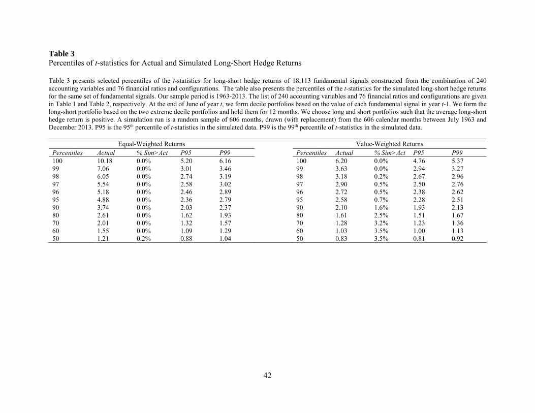
42

Table 3 Percentiles of t-statistics for Actual and Simulated Long-Short Hedge Returns Table 3 presents selected percentiles of the t-statistics for long-short hedge returns of 18,113 fundamental signals constructed from the combination of 240 accounting variables and 76 financial ratios and configurations. The table also presents the percentiles of the t-statistics for the simulated long-short hedge returns for the same set of fundamental signals. Our sample period is 1963-2013. The list of 240 accounting variables and 76 financial ratios and configurations are given in Table 1 and Table 2, respectively. At the end of June of year t, we form decile portfolios based on the value of each fundamental signal in year t-1. We form the long-short portfolio based on the two extreme decile portfolios and hold them for 12 months. We choose long and short portfolios such that the average long-short hedge return is positive. A simulation run is a random sample of 606 months, drawn (with replacement) from the 606 calendar months between July 1963 and December 2013. P95 is the 95th percentile of t-statistics in the simulated data. P99 is the 99th percentile of t-statistics in the simulated data.

Equal-Weighted Returns Value-Weighted ReturnsPercentiles Actual % Sim>Act P95 P99 Percentiles Actual % Sim>Act P95 P99 100 10.18 0.0% 5.20 6.16 100 6.20 0.0% 4.76 5.37 99 7.06 0.0% 3.01 3.46 99 3.63 0.0% 2.94 3.27 98 6.05 0.0% 2.74 3.19 98 3.18 0.2% 2.67 2.96 97 5.54 0.0% 2.58 3.02 97 2.90 0.5% 2.50 2.76 96 5.18 0.0% 2.46 2.89 96 2.72 0.5% 2.38 2.62 95 4.88 0.0% 2.36 2.79 95 2.58 0.7% 2.28 2.51 90 3.74 0.0% 2.03 2.37 90 2.10 1.6% 1.93 2.13 80 2.61 0.0% 1.62 1.93 80 1.61 2.5% 1.51 1.67 70 2.01 0.0% 1.32 1.57 70 1.28 3.2% 1.23 1.36 60 1.55 0.0% 1.09 1.29 60 1.03 3.5% 1.00 1.13 50 1.21 0.2% 0.88 1.04 50 0.83 3.5% 0.81 0.92

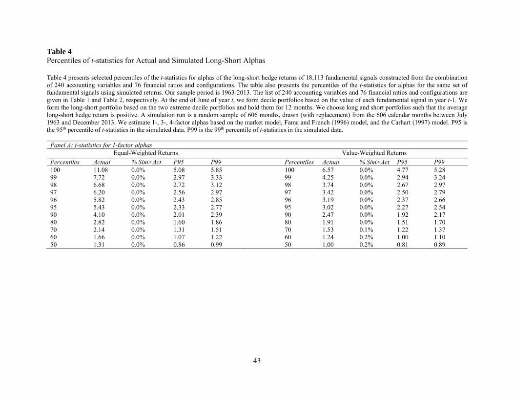
43

Table 4 Percentiles of t-statistics for Actual and Simulated Long-Short Alphas Table 4 presents selected percentiles of the t-statistics for alphas of the long-short hedge returns of 18,113 fundamental signals constructed from the combination of 240 accounting variables and 76 financial ratios and configurations. The table also presents the percentiles of the t-statistics for alphas for the same set of fundamental signals using simulated returns. Our sample period is 1963-2013. The list of 240 accounting variables and 76 financial ratios and configurations are given in Table 1 and Table 2, respectively. At the end of June of year t, we form decile portfolios based on the value of each fundamental signal in year t-1. We form the long-short portfolio based on the two extreme decile portfolios and hold them for 12 months. We choose long and short portfolios such that the average long-short hedge return is positive. A simulation run is a random sample of 606 months, drawn (with replacement) from the 606 calendar months between July 1963 and December 2013. We estimate 1-, 3-, 4-factor alphas based on the market model, Fama and French (1996) model, and the Carhart (1997) model. P95 is the 95th percentile of t-statistics in the simulated data. P99 is the 99th percentile of t-statistics in the simulated data.

Panel A: t-statistics for 1-factor alphas Equal-Weighted Returns Value-Weighted Returns

Percentiles Actual % Sim>Act P95 P99 Percentiles Actual % Sim>Act P95 P99 100 11.08 0.0% 5.08 5.85 100 6.57 0.0% 4.77 5.28 99 7.72 0.0% 2.97 3.33 99 4.25 0.0% 2.94 3.24 98 6.68 0.0% 2.72 3.12 98 3.74 0.0% 2.67 2.97 97 6.20 0.0% 2.56 2.97 97 3.42 0.0% 2.50 2.79 96 5.82 0.0% 2.43 2.85 96 3.19 0.0% 2.37 2.66 95 5.43 0.0% 2.33 2.77 95 3.02 0.0% 2.27 2.54 90 4.10 0.0% 2.01 2.39 90 2.47 0.0% 1.92 2.17 80 2.82 0.0% 1.60 1.86 80 1.91 0.0% 1.51 1.70 70 2.14 0.0% 1.31 1.51 70 1.53 0.1% 1.22 1.37 60 1.66 0.0% 1.07 1.22 60 1.24 0.2% 1.00 1.10 50 1.31 0.0% 0.86 0.99 50 1.00 0.2% 0.81 0.89

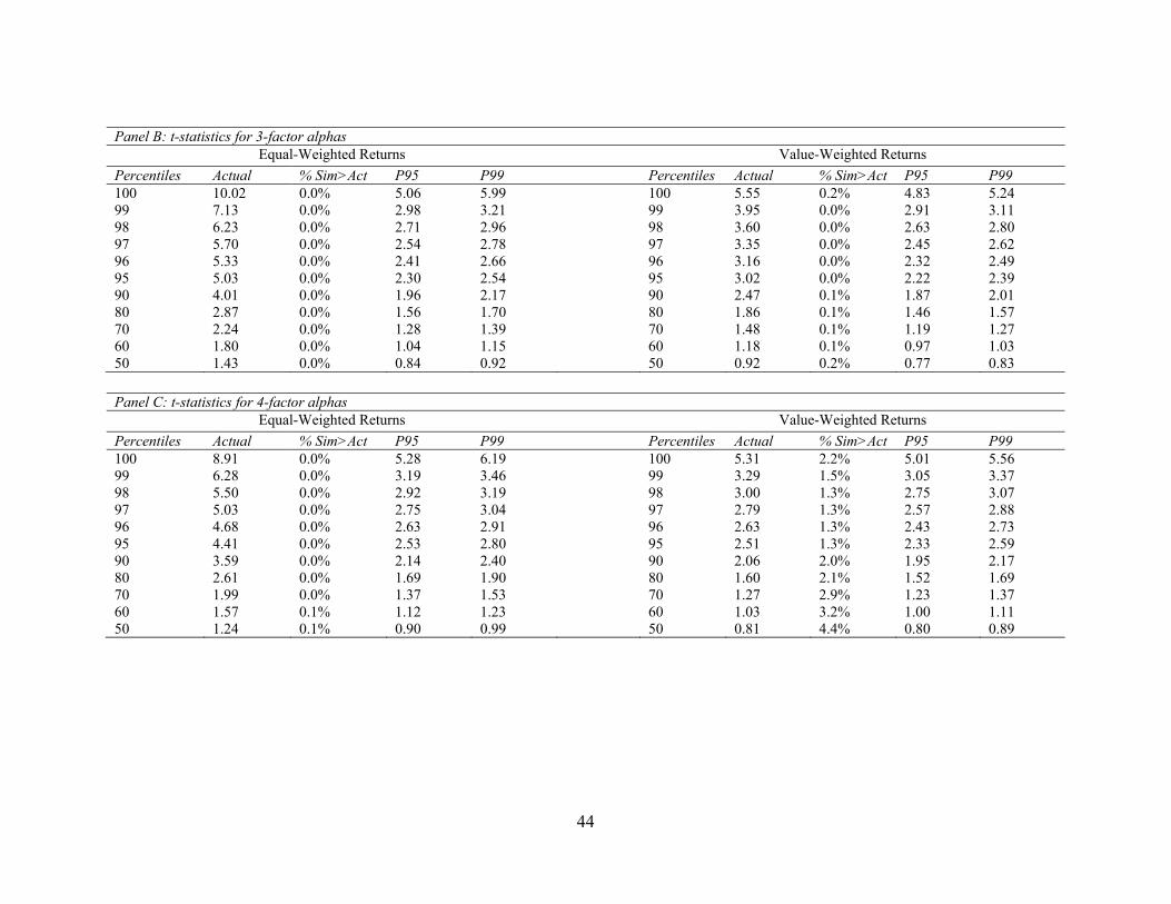
44

Panel B: t-statistics for 3-factor alphas

Equal-Weighted Returns Value-Weighted Returns

Percentiles Actual % Sim>Act P95 P99 Percentiles Actual % Sim>Act P95 P99 100 10.02 0.0% 5.06 5.99 100 5.55 0.2% 4.83 5.24 99 7.13 0.0% 2.98 3.21 99 3.95 0.0% 2.91 3.11 98 6.23 0.0% 2.71 2.96 98 3.60 0.0% 2.63 2.80 97 5.70 0.0% 2.54 2.78 97 3.35 0.0% 2.45 2.62 96 5.33 0.0% 2.41 2.66 96 3.16 0.0% 2.32 2.49 95 5.03 0.0% 2.30 2.54 95 3.02 0.0% 2.22 2.39 90 4.01 0.0% 1.96 2.17 90 2.47 0.1% 1.87 2.01 80 2.87 0.0% 1.56 1.70 80 1.86 0.1% 1.46 1.57 70 2.24 0.0% 1.28 1.39 70 1.48 0.1% 1.19 1.27 60 1.80 0.0% 1.04 1.15 60 1.18 0.1% 0.97 1.03 50 1.43 0.0% 0.84 0.92 50 0.92 0.2% 0.77 0.83

Panel C: t-statistics for 4-factor alphas

Equal-Weighted Returns Value-Weighted Returns

Percentiles Actual % Sim>Act P95 P99 Percentiles Actual % Sim>Act P95 P99 100 8.91 0.0% 5.28 6.19 100 5.31 2.2% 5.01 5.56 99 6.28 0.0% 3.19 3.46 99 3.29 1.5% 3.05 3.37 98 5.50 0.0% 2.92 3.19 98 3.00 1.3% 2.75 3.07 97 5.03 0.0% 2.75 3.04 97 2.79 1.3% 2.57 2.88 96 4.68 0.0% 2.63 2.91 96 2.63 1.3% 2.43 2.73 95 4.41 0.0% 2.53 2.80 95 2.51 1.3% 2.33 2.59 90 3.59 0.0% 2.14 2.40 90 2.06 2.0% 1.95 2.17 80 2.61 0.0% 1.69 1.90 80 1.60 2.1% 1.52 1.69 70 1.99 0.0% 1.37 1.53 70 1.27 2.9% 1.23 1.37 60 1.57 0.1% 1.12 1.23 60 1.03 3.2% 1.00 1.11 50 1.24 0.1% 0.90 0.99 50 0.81 4.4% 0.80 0.89

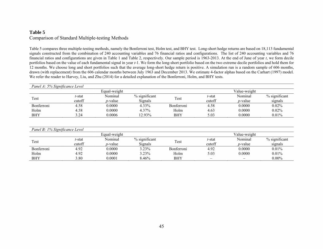
45

Table 5 Comparison of Standard Multiple-testing Methods Table 5 compares three multiple-testing methods, namely the Bonferroni test, Holm test, and BHY test. Long-short hedge returns are based on 18,113 fundamental signals constructed from the combination of 240 accounting variables and 76 financial ratios and configurations. The list of 240 accounting variables and 76 financial ratios and configurations are given in Table 1 and Table 2, respectively. Our sample period is 1963-2013. At the end of June of year t, we form decile portfolios based on the value of each fundamental signal in year t-1. We form the long-short portfolio based on the two extreme decile portfolios and hold them for 12 months. We choose long and short portfolios such that the average long-short hedge return is positive. A simulation run is a random sample of 606 months, drawn (with replacement) from the 606 calendar months between July 1963 and December 2013. We estimate 4-factor alphas based on the Carhart (1997) model. We refer the reader to Harvey, Liu, and Zhu (2014) for a detailed explanation of the Bonferroni, Holm, and BHY tests.

Panel A: 5% Significance Level Equal-weight Value-weight

Test t-stat cutoff

Nominal p-value

% significant Signals

Test t-stat cutoff

Nominal p-value

% significant signals

Bonferroni 4.58 0.0000 4.33% Bonferroni 4.58 0.0000 0.02% Holm 4.58 0.0000 4.37% Holm 4.63 0.0000 0.02% BHY 3.24 0.0006 12.93% BHY 5.03 0.0000 0.01%

Panel B: 1% Significance Level Equal-weight Value-weight

Test t-stat cutoff

Nominal p-value

% significant Signals

Test t-stat cutoff

Nominal p-value

% significant signals

Bonferroni 4.92 0.0000 3.23% Bonferroni 4.92 0.0000 0.01% Holm 4.92 0.0000 3.23% Holm 5.03 0.0000 0.01% BHY 3.80 0.0001 8.46% BHY – – 0.00%

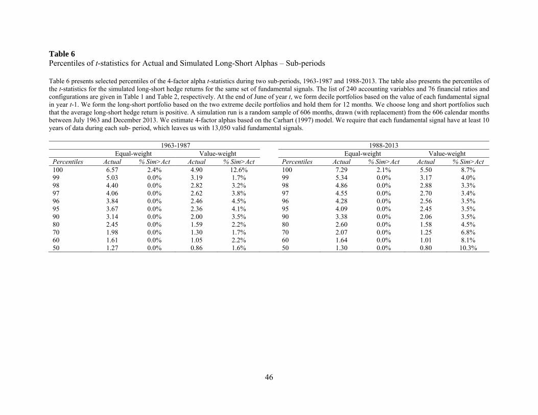
46

Table 6 Percentiles of t-statistics for Actual and Simulated Long-Short Alphas – Sub-periods Table 6 presents selected percentiles of the 4-factor alpha t-statistics during two sub-periods, 1963-1987 and 1988-2013. The table also presents the percentiles of the t-statistics for the simulated long-short hedge returns for the same set of fundamental signals. The list of 240 accounting variables and 76 financial ratios and configurations are given in Table 1 and Table 2, respectively. At the end of June of year t, we form decile portfolios based on the value of each fundamental signal in year t-1. We form the long-short portfolio based on the two extreme decile portfolios and hold them for 12 months. We choose long and short portfolios such that the average long-short hedge return is positive. A simulation run is a random sample of 606 months, drawn (with replacement) from the 606 calendar months between July 1963 and December 2013. We estimate 4-factor alphas based on the Carhart (1997) model. We require that each fundamental signal have at least 10 years of data during each sub- period, which leaves us with 13,050 valid fundamental signals.

1963-1987 1988-2013 Equal-weight Value-weight Equal-weight Value-weight

Percentiles Actual % Sim>Act Actual % Sim>Act Percentiles Actual % Sim>Act Actual % Sim>Act 100 6.57 2.4% 4.90 12.6% 100 7.29 2.1% 5.50 8.7% 99 5.03 0.0% 3.19 1.7% 99 5.34 0.0% 3.17 4.0% 98 4.40 0.0% 2.82 3.2% 98 4.86 0.0% 2.88 3.3% 97 4.06 0.0% 2.62 3.8% 97 4.55 0.0% 2.70 3.4% 96 3.84 0.0% 2.46 4.5% 96 4.28 0.0% 2.56 3.5% 95 3.67 0.0% 2.36 4.1% 95 4.09 0.0% 2.45 3.5% 90 3.14 0.0% 2.00 3.5% 90 3.38 0.0% 2.06 3.5% 80 2.45 0.0% 1.59 2.2% 80 2.60 0.0% 1.58 4.5% 70 1.98 0.0% 1.30 1.7% 70 2.07 0.0% 1.25 6.8% 60 1.61 0.0% 1.05 2.2% 60 1.64 0.0% 1.01 8.1% 50 1.27 0.0% 0.86 1.6% 50 1.30 0.0% 0.80 10.3%

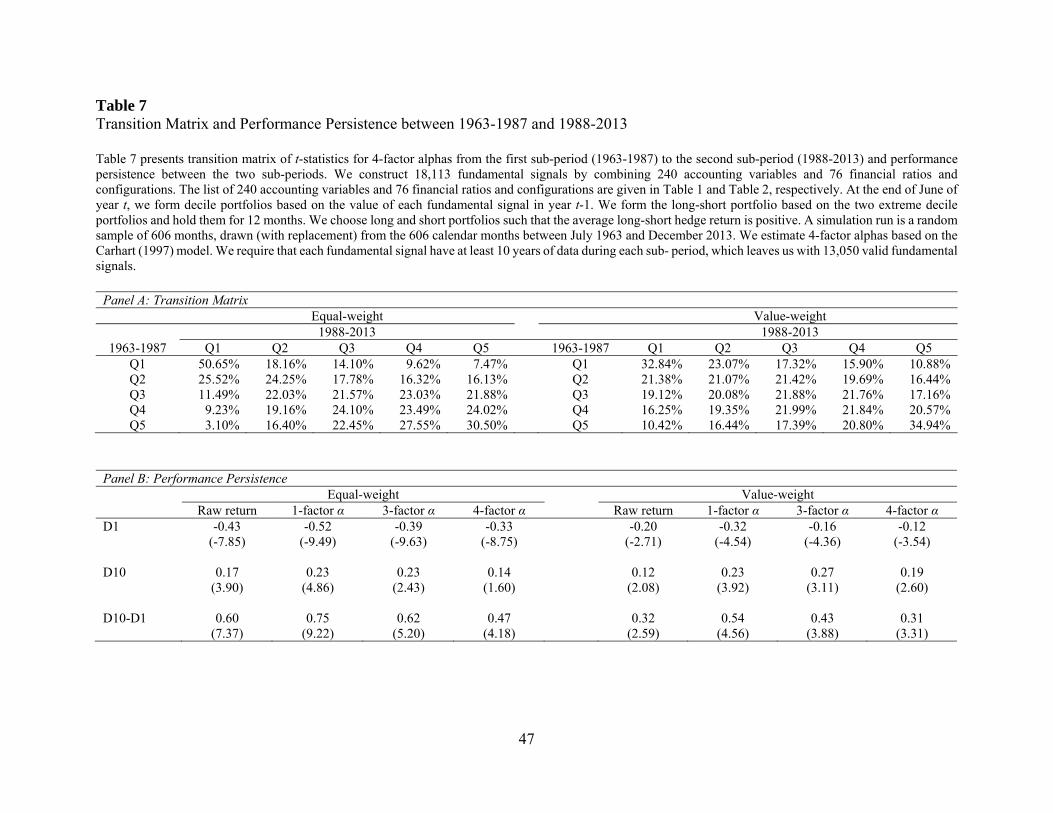
47

Table 7 Transition Matrix and Performance Persistence between 1963-1987 and 1988-2013 Table 7 presents transition matrix of t-statistics for 4-factor alphas from the first sub-period (1963-1987) to the second sub-period (1988-2013) and performance persistence between the two sub-periods. We construct 18,113 fundamental signals by combining 240 accounting variables and 76 financial ratios and configurations. The list of 240 accounting variables and 76 financial ratios and configurations are given in Table 1 and Table 2, respectively. At the end of June of year t, we form decile portfolios based on the value of each fundamental signal in year t-1. We form the long-short portfolio based on the two extreme decile portfolios and hold them for 12 months. We choose long and short portfolios such that the average long-short hedge return is positive. A simulation run is a random sample of 606 months, drawn (with replacement) from the 606 calendar months between July 1963 and December 2013. We estimate 4-factor alphas based on the Carhart (1997) model. We require that each fundamental signal have at least 10 years of data during each sub- period, which leaves us with 13,050 valid fundamental signals.

Panel A: Transition Matrix Equal-weight Value-weight 1988-2013 1988-2013 1963-1987 Q1 Q2 Q3 Q4 Q5 1963-1987 Q1 Q2 Q3 Q4 Q5

Q1 50.65% 18.16% 14.10% 9.62% 7.47% Q1 32.84% 23.07% 17.32% 15.90% 10.88% Q2 25.52% 24.25% 17.78% 16.32% 16.13% Q2 21.38% 21.07% 21.42% 19.69% 16.44% Q3 11.49% 22.03% 21.57% 23.03% 21.88% Q3 19.12% 20.08% 21.88% 21.76% 17.16% Q4 9.23% 19.16% 24.10% 23.49% 24.02% Q4 16.25% 19.35% 21.99% 21.84% 20.57% Q5 3.10% 16.40% 22.45% 27.55% 30.50% Q5 10.42% 16.44% 17.39% 20.80% 34.94%

Panel B: Performance Persistence Equal-weight Value-weight Raw return 1-factor α 3-factor α 4-factor α Raw return 1-factor α 3-factor α 4-factor α D1 -0.43 -0.52 -0.39 -0.33 -0.20 -0.32 -0.16 -0.12 (-7.85) (-9.49) (-9.63) (-8.75) (-2.71) (-4.54) (-4.36) (-3.54) D10 0.17 0.23 0.23 0.14 0.12 0.23 0.27 0.19 (3.90) (4.86) (2.43) (1.60) (2.08) (3.92) (3.11) (2.60) D10-D1 0.60 0.75 0.62 0.47 0.32 0.54 0.43 0.31 (7.37) (9.22) (5.20) (4.18) (2.59) (4.56) (3.88) (3.31)

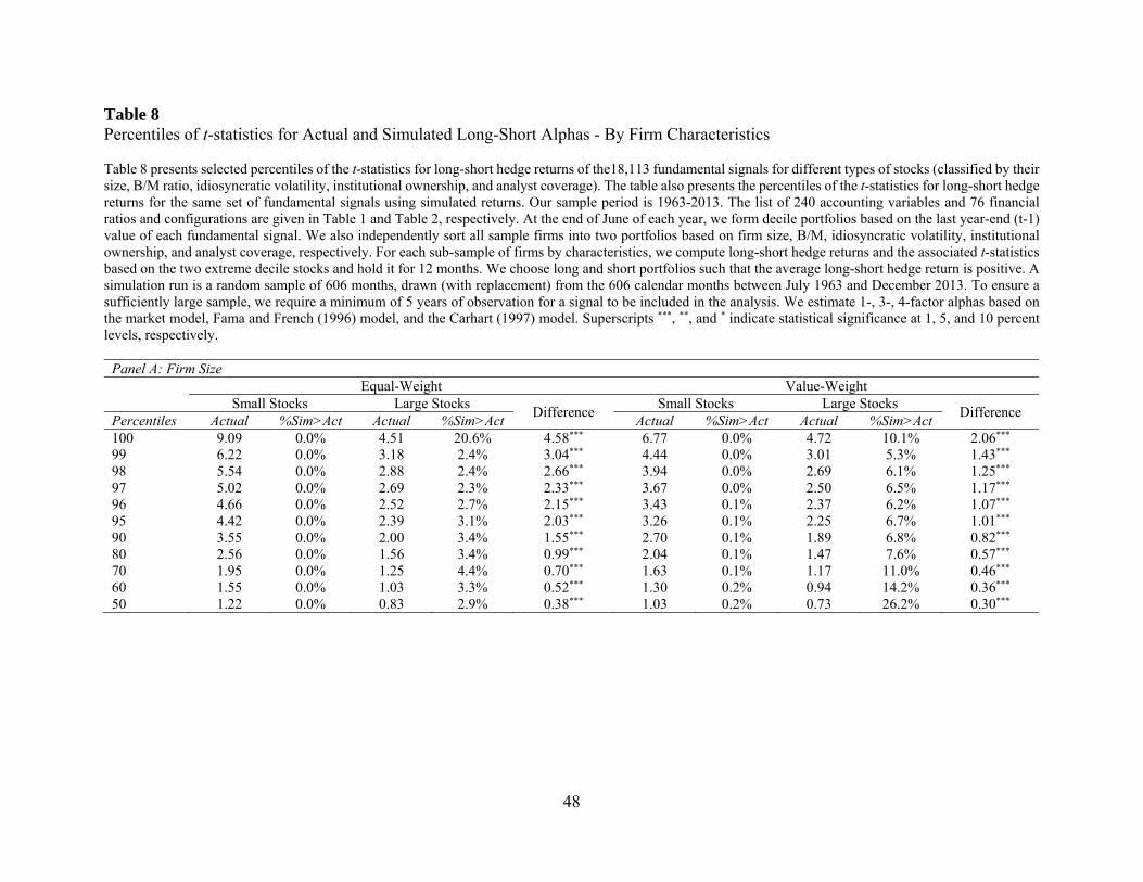
48

Table 8 Percentiles of t-statistics for Actual and Simulated Long-Short Alphas - By Firm Characteristics Table 8 presents selected percentiles of the t-statistics for long-short hedge returns of the18,113 fundamental signals for different types of stocks (classified by their size, B/M ratio, idiosyncratic volatility, institutional ownership, and analyst coverage). The table also presents the percentiles of the t-statistics for long-short hedge returns for the same set of fundamental signals using simulated returns. Our sample period is 1963-2013. The list of 240 accounting variables and 76 financial ratios and configurations are given in Table 1 and Table 2, respectively. At the end of June of each year, we form decile portfolios based on the last year-end (t-1) value of each fundamental signal. We also independently sort all sample firms into two portfolios based on firm size, B/M, idiosyncratic volatility, institutional ownership, and analyst coverage, respectively. For each sub-sample of firms by characteristics, we compute long-short hedge returns and the associated t-statistics based on the two extreme decile stocks and hold it for 12 months. We choose long and short portfolios such that the average long-short hedge return is positive. A simulation run is a random sample of 606 months, drawn (with replacement) from the 606 calendar months between July 1963 and December 2013. To ensure a sufficiently large sample, we require a minimum of 5 years of observation for a signal to be included in the analysis. We estimate 1-, 3-, 4-factor alphas based on the market model, Fama and French (1996) model, and the Carhart (1997) model. Superscripts ***, **, and * indicate statistical significance at 1, 5, and 10 percent levels, respectively.

Panel A: Firm Size Equal-Weight Value-Weight Small Stocks Large Stocks

Difference Small Stocks Large Stocks

Difference Percentiles Actual %Sim>Act Actual %Sim>Act Actual %Sim>Act Actual %Sim>Act 100 9.09 0.0% 4.51 20.6% 4.58*** 6.77 0.0% 4.72 10.1% 2.06*** 99 6.22 0.0% 3.18 2.4% 3.04*** 4.44 0.0% 3.01 5.3% 1.43*** 98 5.54 0.0% 2.88 2.4% 2.66*** 3.94 0.0% 2.69 6.1% 1.25*** 97 5.02 0.0% 2.69 2.3% 2.33*** 3.67 0.0% 2.50 6.5% 1.17*** 96 4.66 0.0% 2.52 2.7% 2.15*** 3.43 0.1% 2.37 6.2% 1.07*** 95 4.42 0.0% 2.39 3.1% 2.03*** 3.26 0.1% 2.25 6.7% 1.01*** 90 3.55 0.0% 2.00 3.4% 1.55*** 2.70 0.1% 1.89 6.8% 0.82*** 80 2.56 0.0% 1.56 3.4% 0.99*** 2.04 0.1% 1.47 7.6% 0.57*** 70 1.95 0.0% 1.25 4.4% 0.70*** 1.63 0.1% 1.17 11.0% 0.46*** 60 1.55 0.0% 1.03 3.3% 0.52*** 1.30 0.2% 0.94 14.2% 0.36*** 50 1.22 0.0% 0.83 2.9% 0.38*** 1.03 0.2% 0.73 26.2% 0.30***

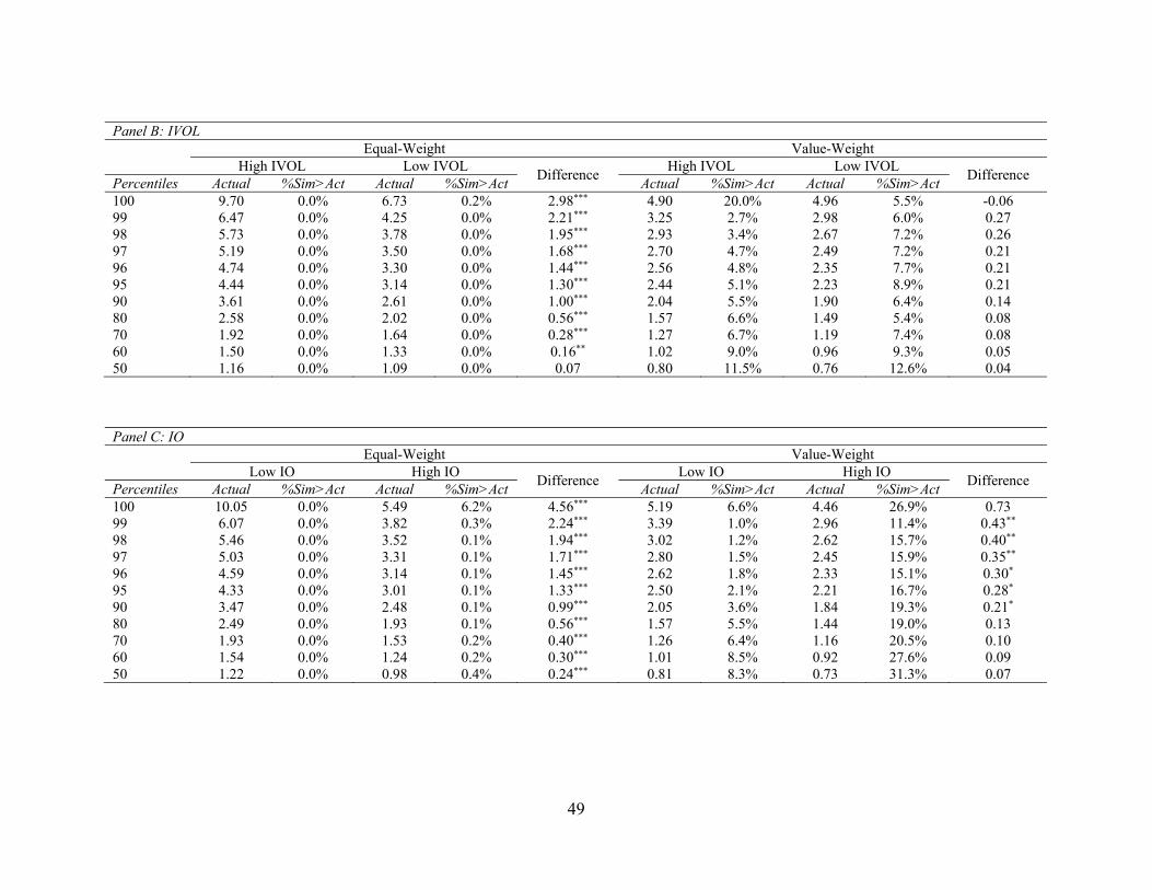
49

Panel B: IVOL

Equal-Weight Value-Weight High IVOL Low IVOL

Difference High IVOL Low IVOL

Difference Percentiles Actual %Sim>Act Actual %Sim>Act Actual %Sim>Act Actual %Sim>Act 100 9.70 0.0% 6.73 0.2% 2.98*** 4.90 20.0% 4.96 5.5% -0.06 99 6.47 0.0% 4.25 0.0% 2.21*** 3.25 2.7% 2.98 6.0% 0.27 98 5.73 0.0% 3.78 0.0% 1.95*** 2.93 3.4% 2.67 7.2% 0.26 97 5.19 0.0% 3.50 0.0% 1.68*** 2.70 4.7% 2.49 7.2% 0.21 96 4.74 0.0% 3.30 0.0% 1.44*** 2.56 4.8% 2.35 7.7% 0.21 95 4.44 0.0% 3.14 0.0% 1.30*** 2.44 5.1% 2.23 8.9% 0.21 90 3.61 0.0% 2.61 0.0% 1.00*** 2.04 5.5% 1.90 6.4% 0.14 80 2.58 0.0% 2.02 0.0% 0.56*** 1.57 6.6% 1.49 5.4% 0.08 70 1.92 0.0% 1.64 0.0% 0.28*** 1.27 6.7% 1.19 7.4% 0.08 60 1.50 0.0% 1.33 0.0% 0.16** 1.02 9.0% 0.96 9.3% 0.05 50 1.16 0.0% 1.09 0.0% 0.07 0.80 11.5% 0.76 12.6% 0.04

Panel C: IO Equal-Weight Value-Weight Low IO High IO

Difference Low IO High IO

Difference Percentiles Actual %Sim>Act Actual %Sim>Act Actual %Sim>Act Actual %Sim>Act 100 10.05 0.0% 5.49 6.2% 4.56*** 5.19 6.6% 4.46 26.9% 0.73 99 6.07 0.0% 3.82 0.3% 2.24*** 3.39 1.0% 2.96 11.4% 0.43** 98 5.46 0.0% 3.52 0.1% 1.94*** 3.02 1.2% 2.62 15.7% 0.40** 97 5.03 0.0% 3.31 0.1% 1.71*** 2.80 1.5% 2.45 15.9% 0.35** 96 4.59 0.0% 3.14 0.1% 1.45*** 2.62 1.8% 2.33 15.1% 0.30* 95 4.33 0.0% 3.01 0.1% 1.33*** 2.50 2.1% 2.21 16.7% 0.28* 90 3.47 0.0% 2.48 0.1% 0.99*** 2.05 3.6% 1.84 19.3% 0.21* 80 2.49 0.0% 1.93 0.1% 0.56*** 1.57 5.5% 1.44 19.0% 0.13 70 1.93 0.0% 1.53 0.2% 0.40*** 1.26 6.4% 1.16 20.5% 0.10 60 1.54 0.0% 1.24 0.2% 0.30*** 1.01 8.5% 0.92 27.6% 0.09 50 1.22 0.0% 0.98 0.4% 0.24*** 0.81 8.3% 0.73 31.3% 0.07

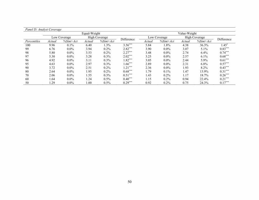
50

Panel D: Analyst Coverage

Equal-Weight Value-Weight Low Coverage High Coverage

Difference Low Coverage High Coverage

Difference Percentiles Actual %Sim>Act Actual %Sim>Act Actual %Sim>Act Actual %Sim>Act 100 9.96 0.1% 6.40 1.3% 3.56*** 5.84 1.8% 4.38 36.3% 1.45* 99 6.76 0.0% 3.94 0.2% 2.82*** 3.90 0.0% 3.07 5.1% 0.83*** 98 5.80 0.0% 3.53 0.2% 2.27*** 3.48 0.0% 2.74 6.4% 0.74*** 97 5.30 0.0% 3.28 0.3% 2.02*** 3.25 0.0% 2.57 6.1% 0.68*** 96 4.92 0.0% 3.11 0.3% 1.82*** 3.05 0.0% 2.44 5.9% 0.61*** 95 4.63 0.0% 2.97 0.3% 1.66*** 2.89 0.0% 2.31 6.8% 0.57*** 90 3.72 0.0% 2.51 0.2% 1.21*** 2.36 0.0% 1.93 8.2% 0.43*** 80 2.64 0.0% 1.95 0.2% 0.68*** 1.79 0.1% 1.47 13.9% 0.31*** 70 2.06 0.0% 1.55 0.3% 0.51*** 1.43 0.2% 1.17 18.7% 0.26*** 60 1.64 0.0% 1.24 0.5% 0.40*** 1.15 0.2% 0.94 22.4% 0.21*** 50 1.29 0.0% 1.00 0.5% 0.29*** 0.92 0.2% 0.75 24.3% 0.17***

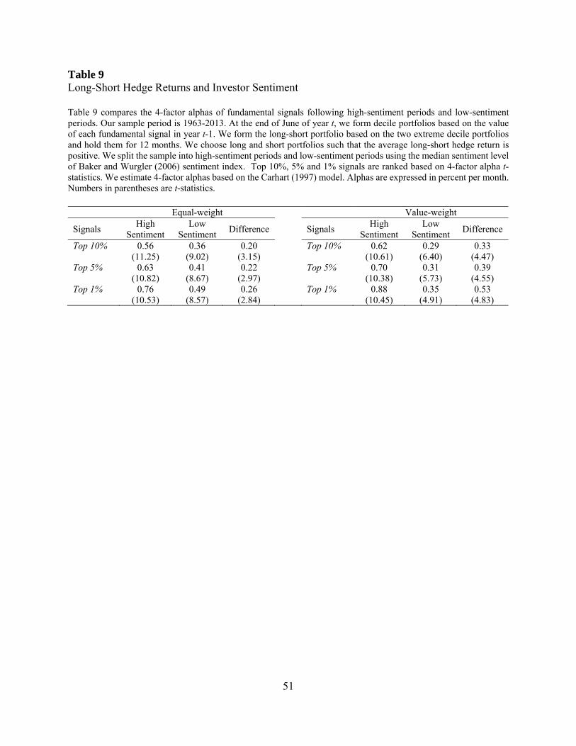
51

Table 9 Long-Short Hedge Returns and Investor Sentiment Table 9 compares the 4-factor alphas of fundamental signals following high-sentiment periods and low-sentiment periods. Our sample period is 1963-2013. At the end of June of year t, we form decile portfolios based on the value of each fundamental signal in year t-1. We form the long-short portfolio based on the two extreme decile portfolios and hold them for 12 months. We choose long and short portfolios such that the average long-short hedge return is positive. We split the sample into high-sentiment periods and low-sentiment periods using the median sentiment level of Baker and Wurgler (2006) sentiment index. Top 10%, 5% and 1% signals are ranked based on 4-factor alpha t-statistics. We estimate 4-factor alphas based on the Carhart (1997) model. Alphas are expressed in percent per month. Numbers in parentheses are t-statistics.

Equal-weight Value-weight

Signals High

Sentiment Low

Sentiment Difference Signals

High Sentiment

Low Sentiment

Difference

Top 10% 0.56 0.36 0.20 Top 10% 0.62 0.29 0.33 (11.25) (9.02) (3.15) (10.61) (6.40) (4.47) Top 5% 0.63 0.41 0.22 Top 5% 0.70 0.31 0.39 (10.82) (8.67) (2.97) (10.38) (5.73) (4.55) Top 1% 0.76 0.49 0.26 Top 1% 0.88 0.35 0.53 (10.53) (8.57) (2.84) (10.45) (4.91) (4.83)

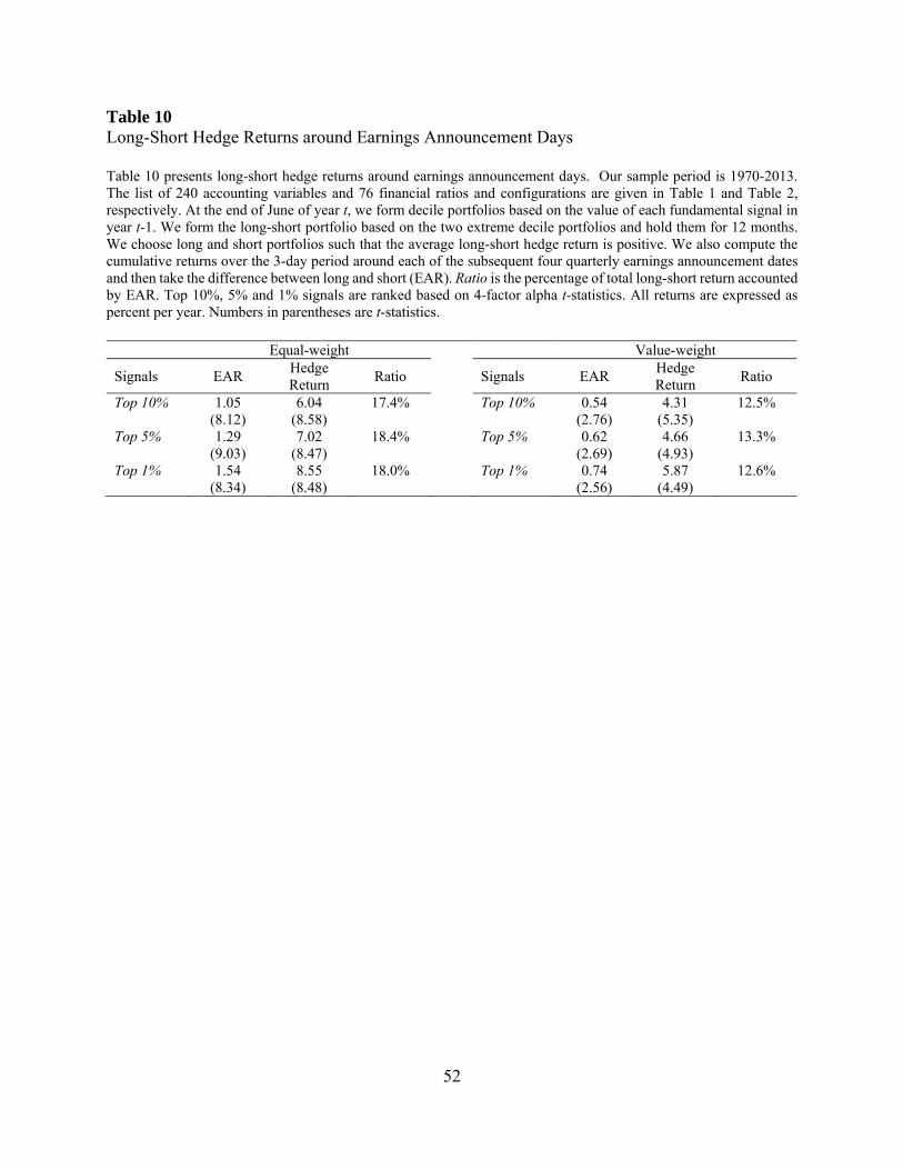
52

Table 10 Long-Short Hedge Returns around Earnings Announcement Days Table 10 presents long-short hedge returns around earnings announcement days. Our sample period is 1970-2013. The list of 240 accounting variables and 76 financial ratios and configurations are given in Table 1 and Table 2, respectively. At the end of June of year t, we form decile portfolios based on the value of each fundamental signal in year t-1. We form the long-short portfolio based on the two extreme decile portfolios and hold them for 12 months. We choose long and short portfolios such that the average long-short hedge return is positive. We also compute the cumulative returns over the 3-day period around each of the subsequent four quarterly earnings announcement dates and then take the difference between long and short (EAR). Ratio is the percentage of total long-short return accounted by EAR. Top 10%, 5% and 1% signals are ranked based on 4-factor alpha t-statistics. All returns are expressed as percent per year. Numbers in parentheses are t-statistics.

Equal-weight Value-weight

Signals EAR Hedge Return

Ratio Signals EAR Hedge Return

Ratio

Top 10% 1.05 6.04 17.4% Top 10% 0.54 4.31 12.5% (8.12) (8.58) (2.76) (5.35) Top 5% 1.29 7.02 18.4% Top 5% 0.62 4.66 13.3% (9.03) (8.47) (2.69) (4.93) Top 1% 1.54 8.55 18.0% Top 1% 0.74 5.87 12.6% (8.34) (8.48) (2.56) (4.49)

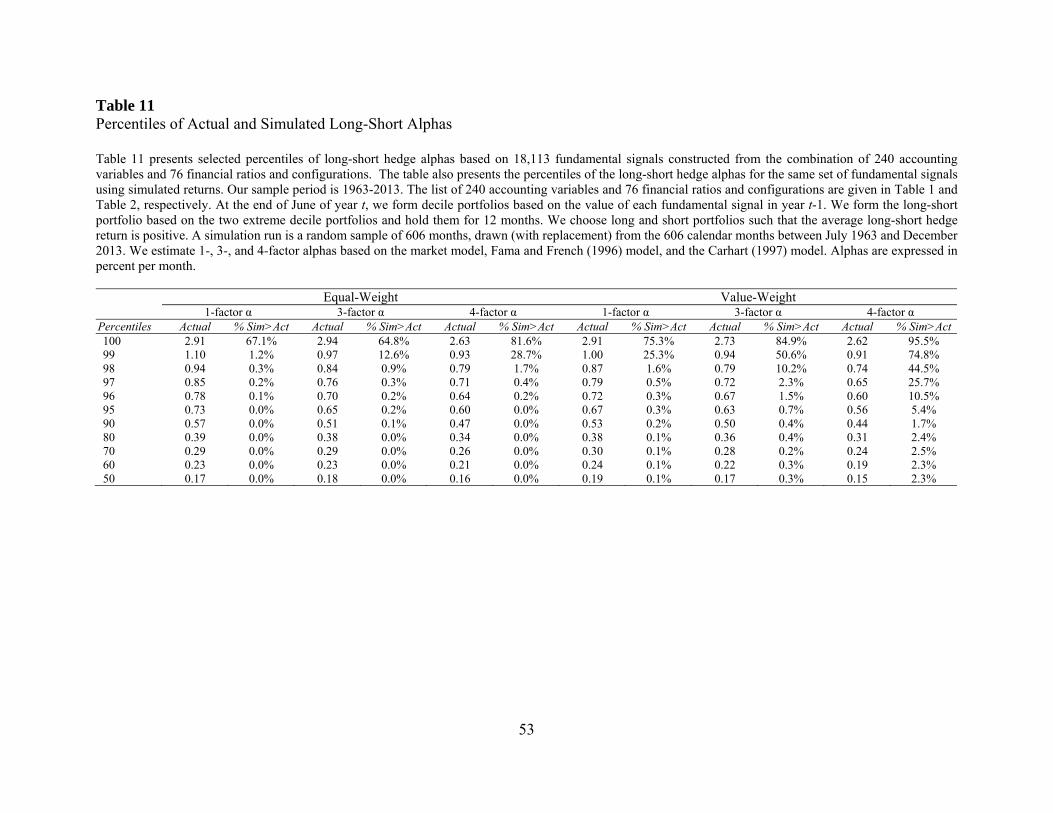
53

Table 11 Percentiles of Actual and Simulated Long-Short Alphas Table 11 presents selected percentiles of long-short hedge alphas based on 18,113 fundamental signals constructed from the combination of 240 accounting variables and 76 financial ratios and configurations. The table also presents the percentiles of the long-short hedge alphas for the same set of fundamental signals using simulated returns. Our sample period is 1963-2013. The list of 240 accounting variables and 76 financial ratios and configurations are given in Table 1 and Table 2, respectively. At the end of June of year t, we form decile portfolios based on the value of each fundamental signal in year t-1. We form the long-short portfolio based on the two extreme decile portfolios and hold them for 12 months. We choose long and short portfolios such that the average long-short hedge return is positive. A simulation run is a random sample of 606 months, drawn (with replacement) from the 606 calendar months between July 1963 and December 2013. We estimate 1-, 3-, and 4-factor alphas based on the market model, Fama and French (1996) model, and the Carhart (1997) model. Alphas are expressed in percent per month.

Equal-Weight Value-Weight 1-factor α 3-factor α 4-factor α 1-factor α 3-factor α 4-factor α

Percentiles Actual % Sim>Act Actual % Sim>Act Actual % Sim>Act Actual % Sim>Act Actual % Sim>Act Actual % Sim>Act100 2.91 67.1% 2.94 64.8% 2.63 81.6% 2.91 75.3% 2.73 84.9% 2.62 95.5% 99 1.10 1.2% 0.97 12.6% 0.93 28.7% 1.00 25.3% 0.94 50.6% 0.91 74.8% 98 0.94 0.3% 0.84 0.9% 0.79 1.7% 0.87 1.6% 0.79 10.2% 0.74 44.5% 97 0.85 0.2% 0.76 0.3% 0.71 0.4% 0.79 0.5% 0.72 2.3% 0.65 25.7% 96 0.78 0.1% 0.70 0.2% 0.64 0.2% 0.72 0.3% 0.67 1.5% 0.60 10.5% 95 0.73 0.0% 0.65 0.2% 0.60 0.0% 0.67 0.3% 0.63 0.7% 0.56 5.4% 90 0.57 0.0% 0.51 0.1% 0.47 0.0% 0.53 0.2% 0.50 0.4% 0.44 1.7% 80 0.39 0.0% 0.38 0.0% 0.34 0.0% 0.38 0.1% 0.36 0.4% 0.31 2.4% 70 0.29 0.0% 0.29 0.0% 0.26 0.0% 0.30 0.1% 0.28 0.2% 0.24 2.5% 60 0.23 0.0% 0.23 0.0% 0.21 0.0% 0.24 0.1% 0.22 0.3% 0.19 2.3% 50 0.17 0.0% 0.18 0.0% 0.16 0.0% 0.19 0.1% 0.17 0.3% 0.15 2.3%