Page 1

Optimization Theory MMC 52212 / MME 52106

by

Dr. Shibayan Sarkar Department of Mechanical Engg. Indian School of Mines Dhanbad

1. Introduction 2. Single Variable Optimization

Page 2

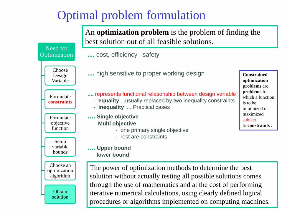
Optimal problem formulation

Need for Optimization

Choose Design Variable

Formulate constraints

Formulate objective function

Setup variable bounds

Choose an optimization

algorithm

Obtain solution

.... cost, efficiency , safety

.... high sensitive to proper working design

.... represents functional relationship between design variable : - equality....usually replaced by two inequality constraints - inequality .... Practical cases .... Single objective Multi objective - one primary single objective - rest are constraints

.... Upper bound lower bound

An optimization problem is the problem of finding the best solution out of all feasible solutions.

The power of optimization methods to determine the best solution without actually testing all possible solutions comes through the use of mathematics and at the cost of performing iterative numerical calculations, using clearly defined logical procedures or algorithms implemented on computing machines.

Constrained optimization problems are problems for which a function is to be minimized or maximized subject to constraints .

Page 3

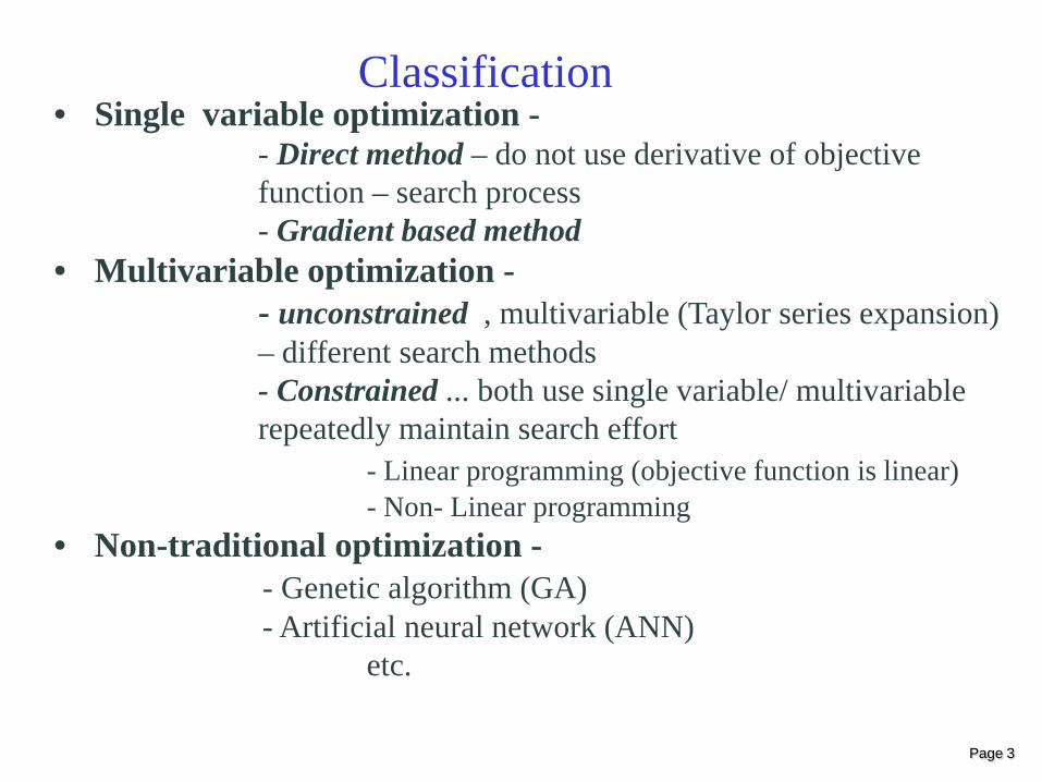
Classification • Single variable optimization -

- Direct method – do not use derivative of objective function – search process - Gradient based method

• Multivariable optimization - - unconstrained , multivariable (Taylor series expansion)

– different search methods - Constrained ... both use single variable/ multivariable

repeatedly maintain search effort - Linear programming (objective function is linear) - Non- Linear programming

• Non-traditional optimization - - Genetic algorithm (GA) - Artificial neural network (ANN) etc.

Page 4

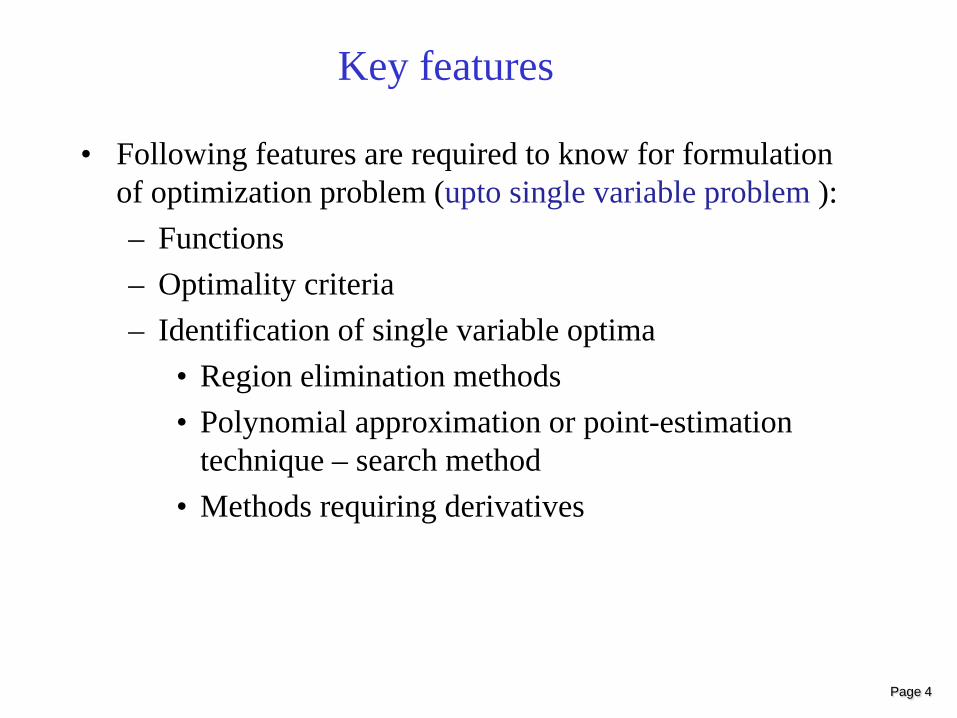
Key features

• Following features are required to know for formulation of optimization problem (upto single variable problem ): – Functions – Optimality criteria – Identification of single variable optima

• Region elimination methods • Polynomial approximation or point-estimation

technique – search method • Methods requiring derivatives

Page 5

Function

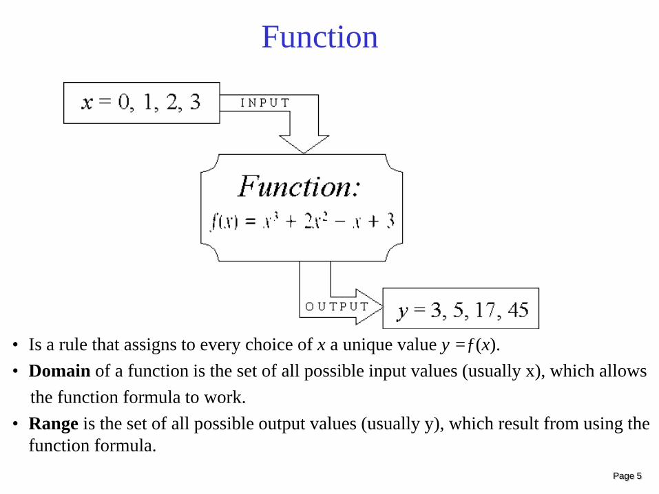
• Is a rule that assigns to every choice of x a unique value y =ƒ(x). • Domain of a function is the set of all possible input values (usually x), which allows the function formula to work. • Range is the set of all possible output values (usually y), which result from using the

function formula.

Page 6

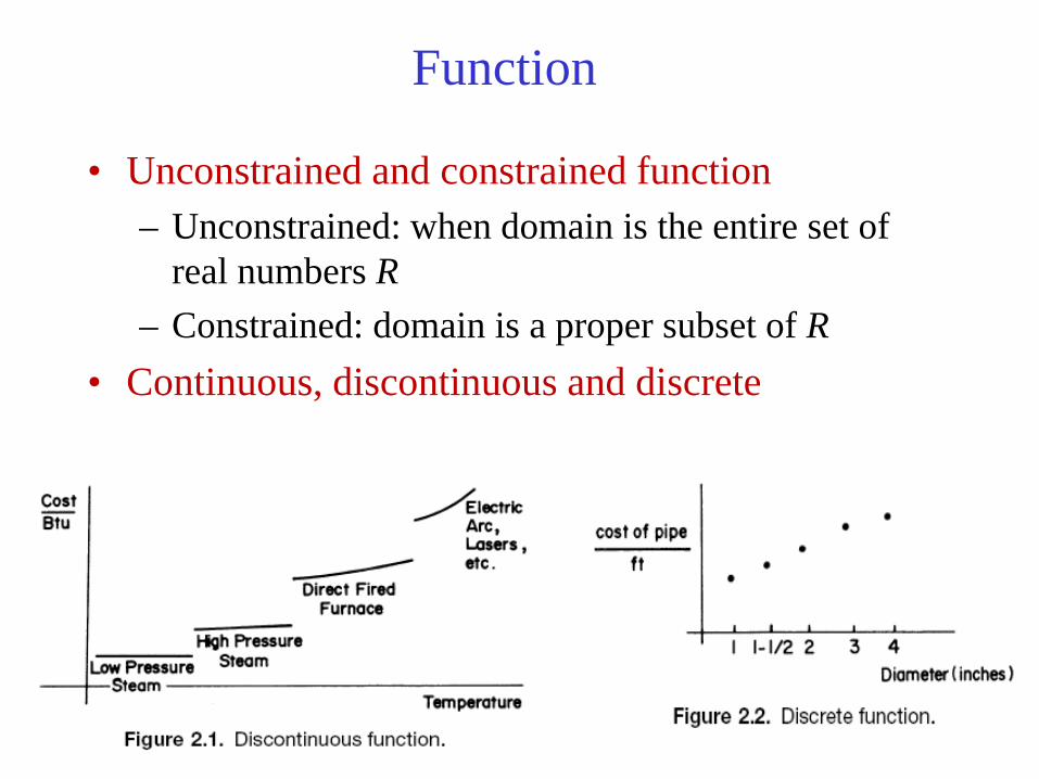
• Unconstrained and constrained function – Unconstrained: when domain is the entire set of

real numbers R – Constrained: domain is a proper subset of R

• Continuous, discontinuous and discrete

Function

Page 7

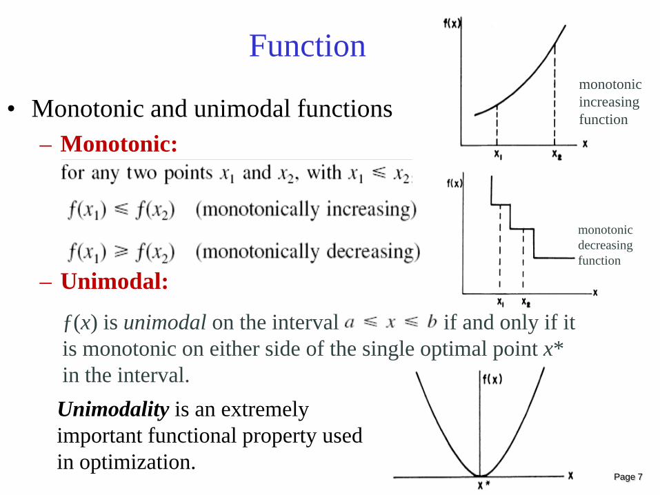
• Monotonic and unimodal functions – Monotonic:

– Unimodal:

Function

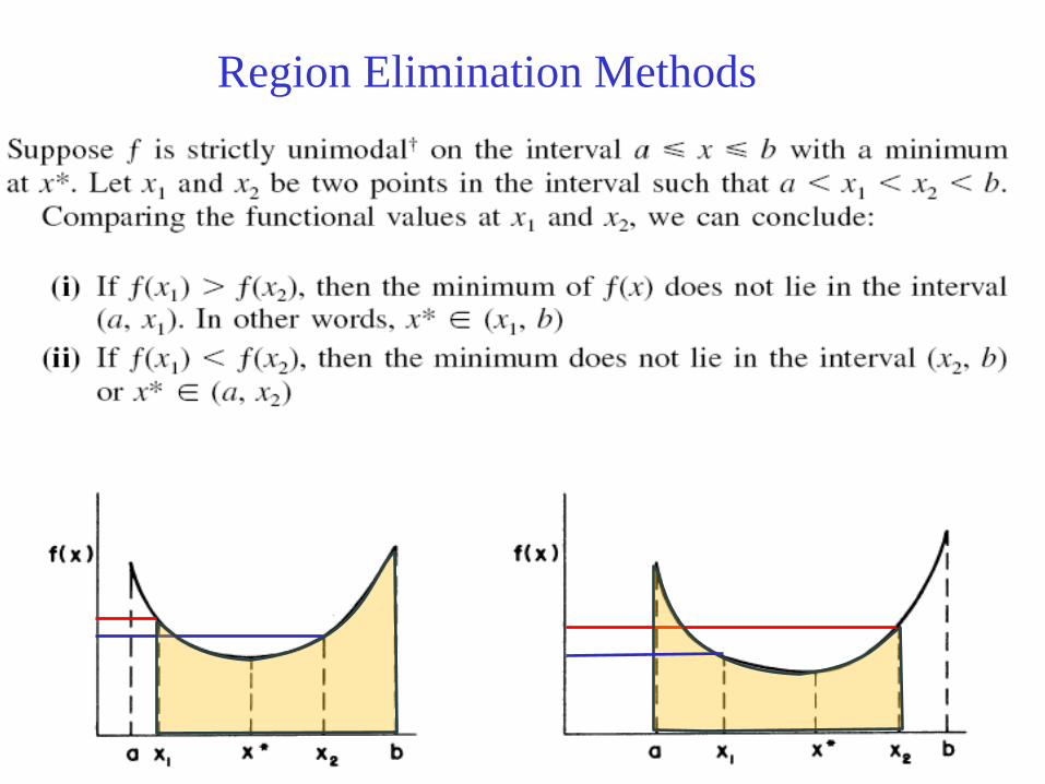
ƒ(x) is unimodal on the interval if and only if it is monotonic on either side of the single optimal point x* in the interval. Unimodality is an extremely important functional property used in optimization.

monotonic decreasing function

monotonic increasing function

Page 8

Optimality Criteria In considering optimization problems, two questions generally must be addressed: • Static Optimization- How can one determine whether a given

point x* is the optimal solution? It refers to the process of minimizing or maximizing the costs/benefits of some objective function for one instant in time only.

• Dynamic Question- If x* is not the optimal point, then how does one go about finding a solution that is optimal? It refers to the process of minimizing or maximizing the costs/benefits of some objective function over a period of time. Sometimes called optimal control. Ex. Calculus of Variation, Optimal Control, Static Optimization to solve dynamic optimization problems etc.

We are mainly concern primarily with the static question, like developing a set of optimality criteria for determining whether a given solution is optimal.

Page 9

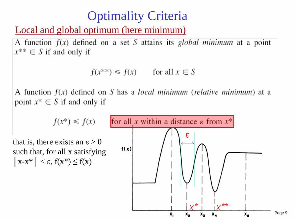
Local and global optimum (here minimum) Optimality Criteria

that is, there exists an ε > 0 such that, for all x satisfying │x-x*│ < ε, f(x*) ≤ f(x)

Page 10

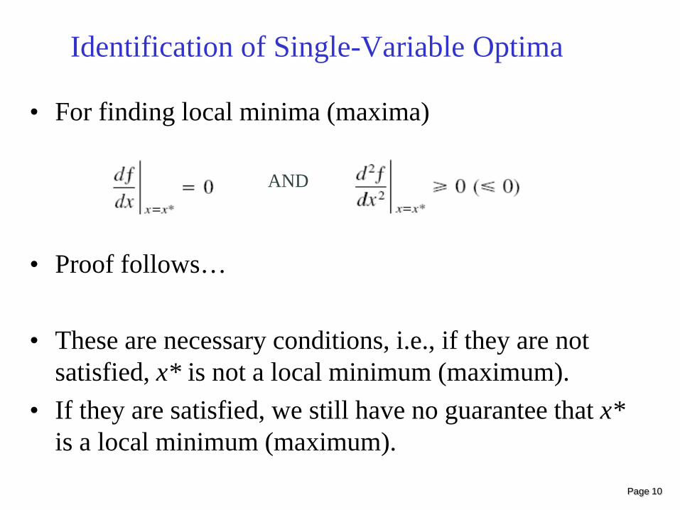
Identification of Single-Variable Optima

• For finding local minima (maxima)

• Proof follows…

• These are necessary conditions, i.e., if they are not satisfied, x* is not a local minimum (maximum).

• If they are satisfied, we still have no guarantee that x* is a local minimum (maximum).

AND

Page 11

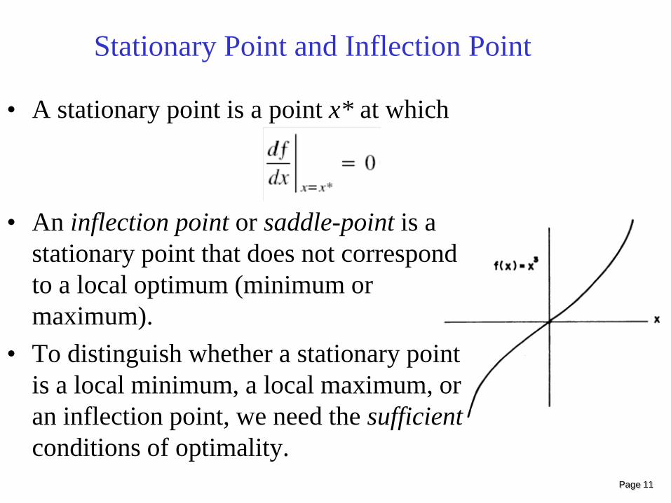
Stationary Point and Inflection Point

• A stationary point is a point x* at which

• An inflection point or saddle-point is a stationary point that does not correspond to a local optimum (minimum or maximum).

• To distinguish whether a stationary point is a local minimum, a local maximum, or an inflection point, we need the sufficient conditions of optimality.

Page 12

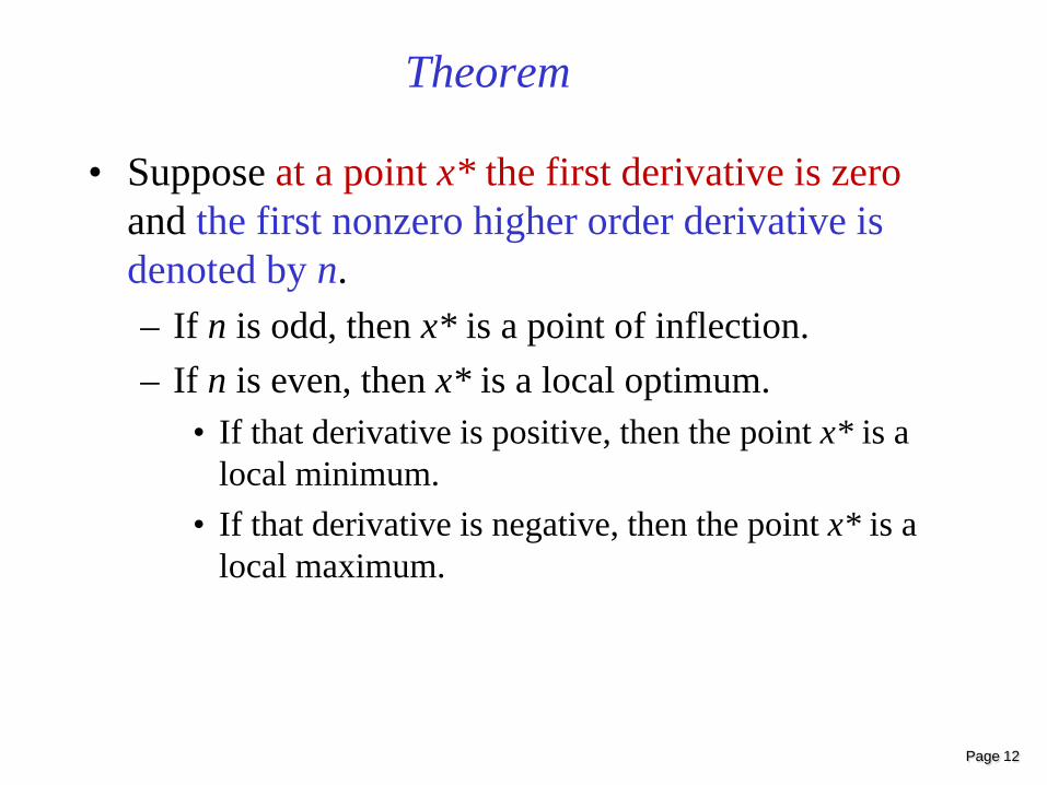
Theorem

• Suppose at a point x* the first derivative is zero and the first nonzero higher order derivative is denoted by n. – If n is odd, then x* is a point of inflection. – If n is even, then x* is a local optimum.

• If that derivative is positive, then the point x* is a local minimum.

• If that derivative is negative, then the point x* is a local maximum.

Page 13

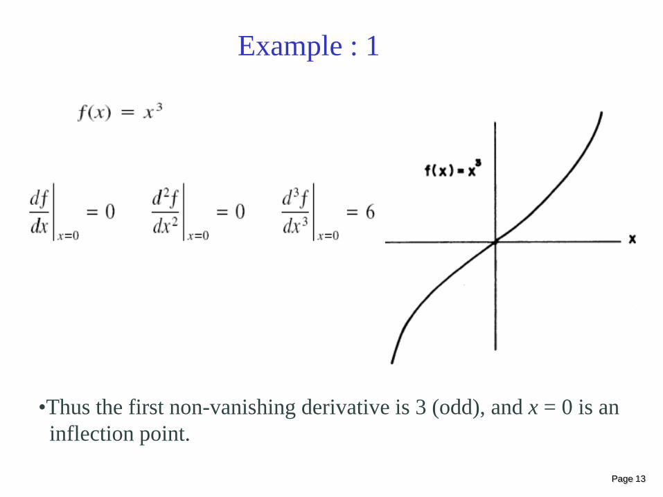
Example : 1

•Thus the first non-vanishing derivative is 3 (odd), and x = 0 is an inflection point.

Page 14

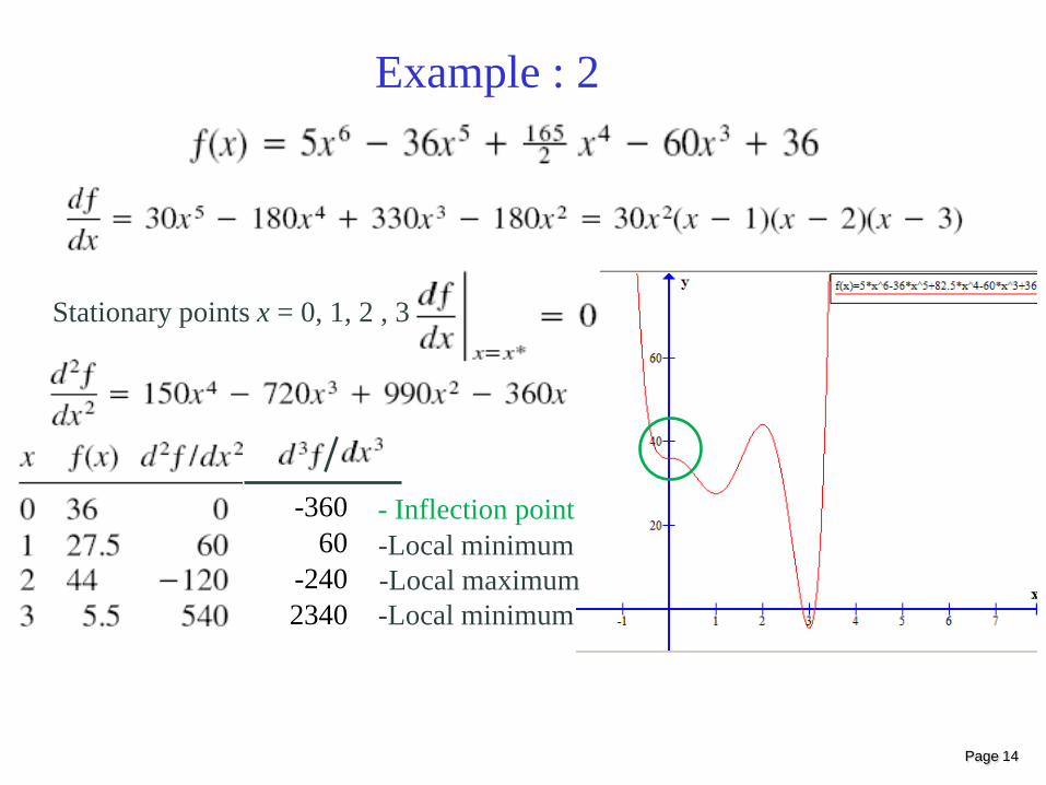
Example : 2

-Local minimum

-Local minimum -Local maximum

Stationary points x = 0, 1, 2 , 3

-360 60

-240 2340

- Inflection point

Page 15

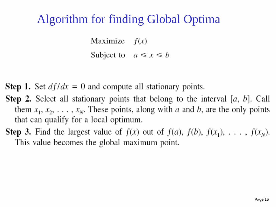
Algorithm for finding Global Optima

Page 16

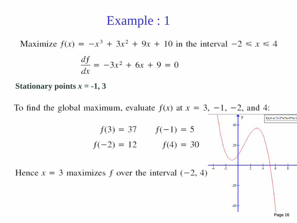
Example : 1

Stationary points x = -1, 3

Page 17

Region Elimination Methods

Page 18

• Bounding Phase – An initial coarse search that will bound or bracket the

optimum • Interval Refinement Phase

– A finite sequence of interval reductions or refinements to reduce the initial search interval to desired accuracy

Region Elimination Methods

How to select x1 and x2 ?

Page 19

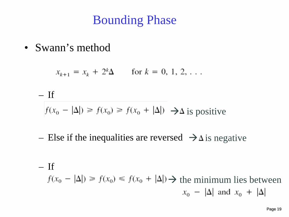
Bounding Phase

• Swann’s method – If

– Else if the inequalities are reversed

– If

is positive

is negative

the minimum lies between

Page 20

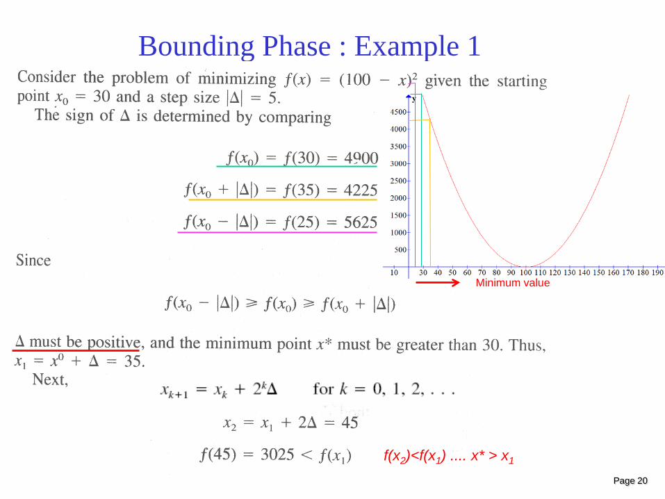
Bounding Phase : Example 1

Minimum value

f(x2)<f(x1) .... x* > x1

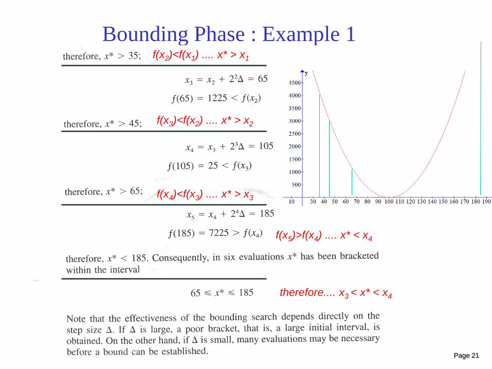
Page 21

Bounding Phase : Example 1 f(x2)<f(x1) .... x* > x1

f(x3)<f(x2) .... x* > x2

f(x4)<f(x3) .... x* > x3

f(x5)>f(x4) .... x* < x4

therefore.... x3 < x* < x4

Page 22

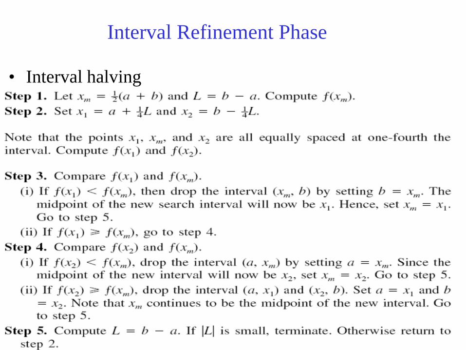
Interval Refinement Phase

• Interval halving

Page 23

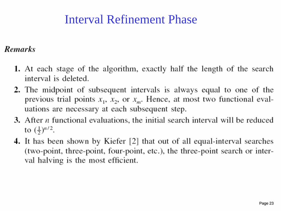
Interval Refinement Phase

Page 24

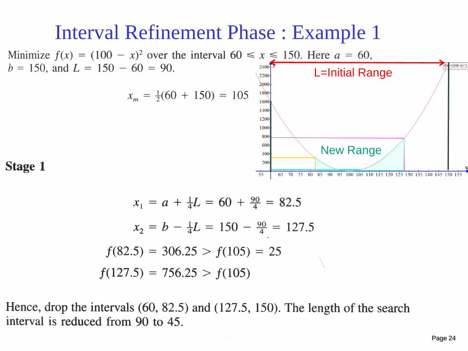
Interval Refinement Phase : Example 1

L=Initial Range

New Range

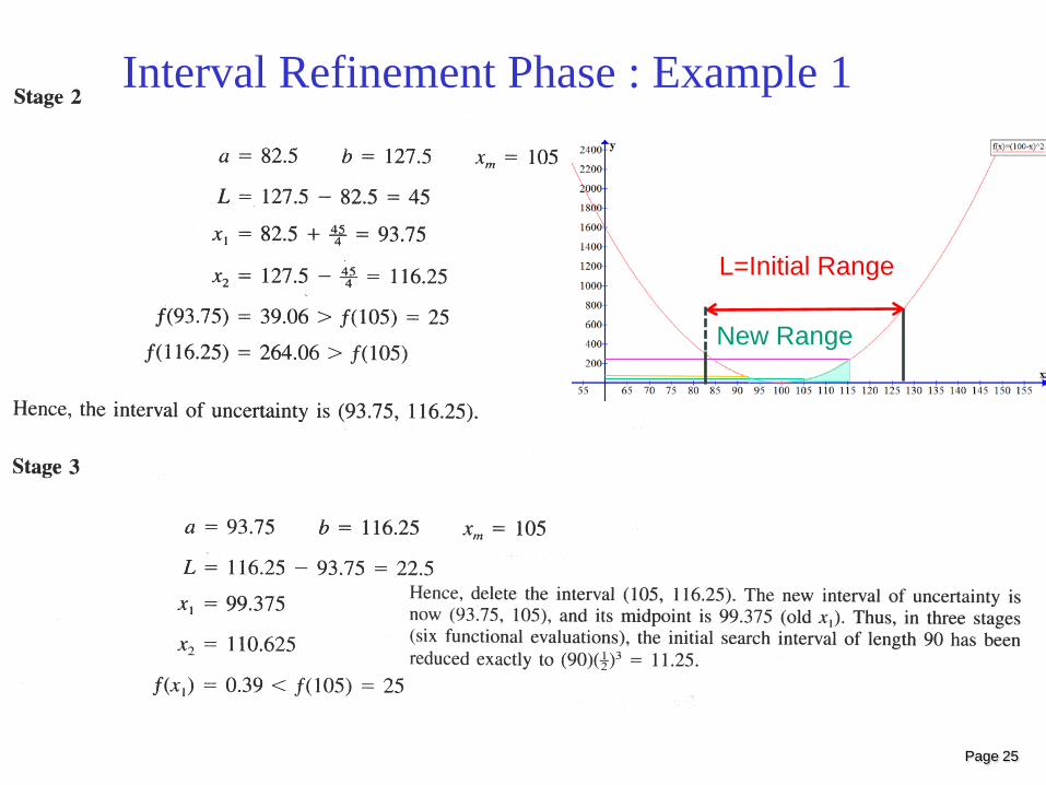
Page 25

Interval Refinement Phase : Example 1

L=Initial Range

New Range

Page 26

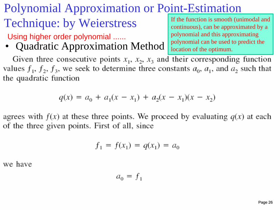
Polynomial Approximation or Point-Estimation Technique: by Weierstress

• Quadratic Approximation Method

If the function is smooth (unimodal and continuous), can be approximated by a polynomial and this approximating polynomial can be used to predict the location of the optimum.

Using higher order polynomial ......

Page 27

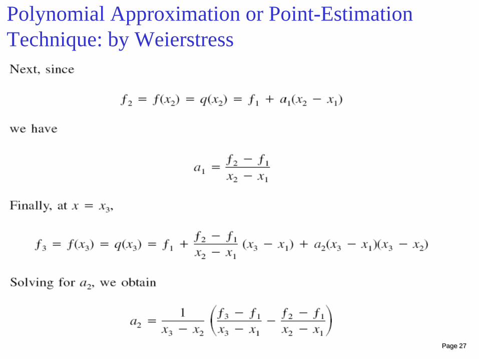
Polynomial Approximation or Point-Estimation Technique: by Weierstress

Page 28

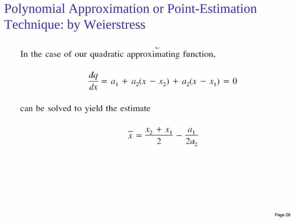
Polynomial Approximation or Point-Estimation Technique: by Weierstress

Page 29

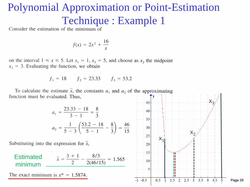
Polynomial Approximation or Point-Estimation Technique : Example 1

Estimated minimum

x1

x2

x3

Page 30

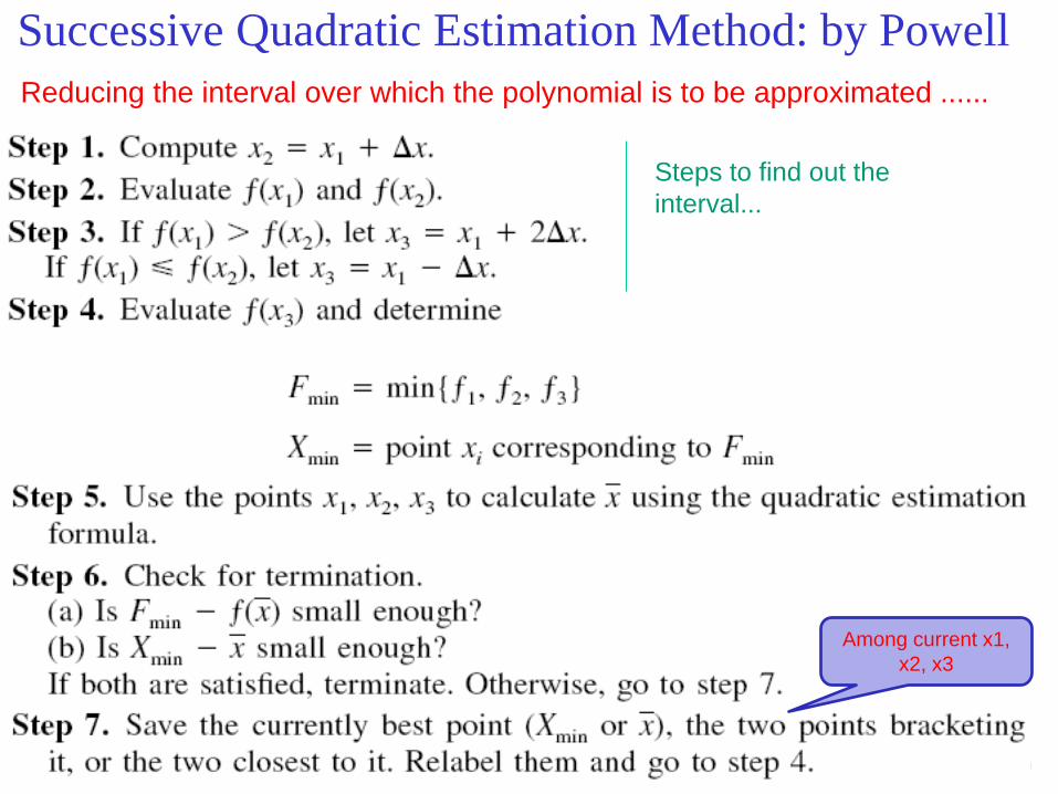
Successive Quadratic Estimation Method: by Powell

Steps to find out the interval...

Reducing the interval over which the polynomial is to be approximated ......

Among current x1, x2, x3

Page 31

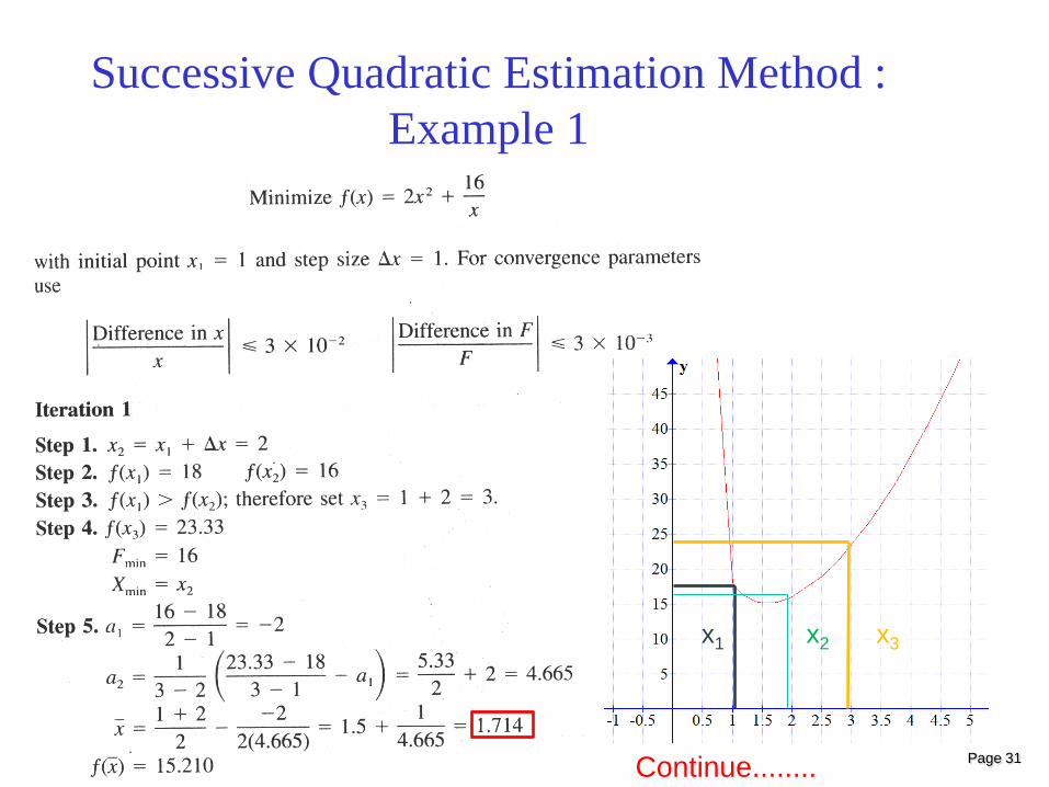
Successive Quadratic Estimation Method : Example 1

Continue........

x1 x2 x3

Page 32

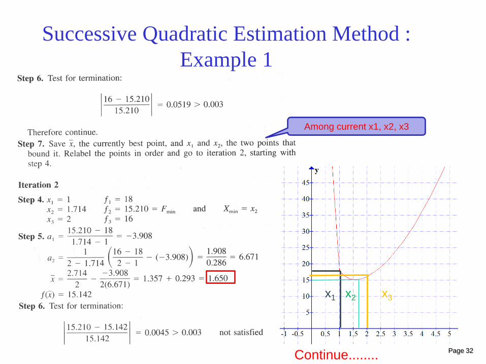
Successive Quadratic Estimation Method : Example 1

Continue........

x1 x2 x3

Among current x1, x2, x3

Page 33

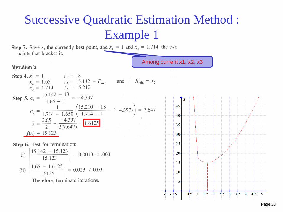
Successive Quadratic Estimation Method : Example 1

Among current x1, x2, x3

Page 34

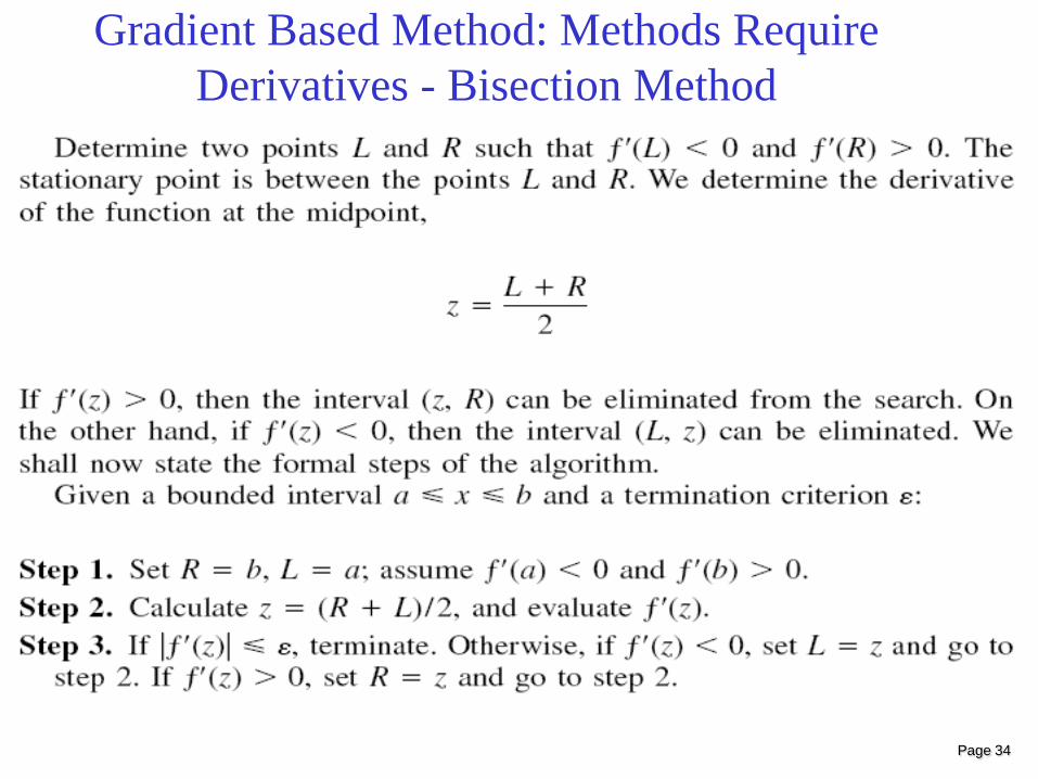
Gradient Based Method: Methods Require Derivatives - Bisection Method

Page 35

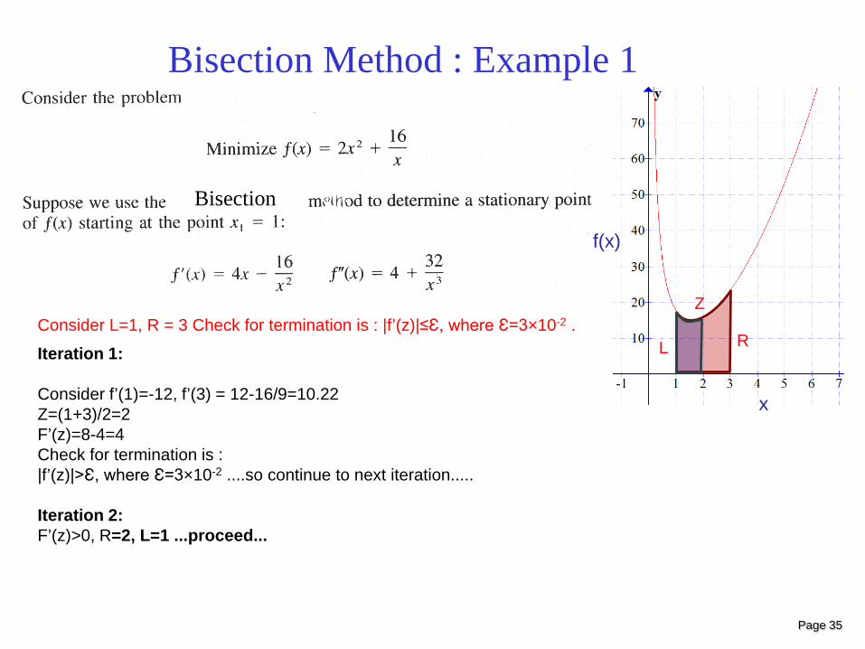
Bisection Method : Example 1

Consider L=1, R = 3 Check for termination is : |f’(z)|≤Ɛ, where Ɛ=3×10-2 .

Iteration 1: Consider f’(1)=-12, f’(3) = 12-16/9=10.22 Z=(1+3)/2=2 F’(z)=8-4=4 Check for termination is : |f’(z)|>Ɛ, where Ɛ=3×10-2 ....so continue to next iteration..... Iteration 2: F’(z)>0, R=2, L=1 ...proceed...

f(x)

x

L R

Z

Bisection

Page 36

Gradient Based Method: Newton-Raphson

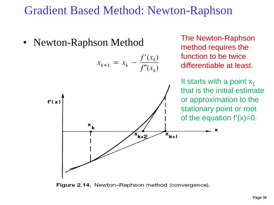
• Newton-Raphson Method The Newton-Raphson method requires the function to be twice differentiable at least.

It starts with a point x1 that is the initial estimate or approximation to the stationary point or root of the equation f’(x)=0.

Page 37

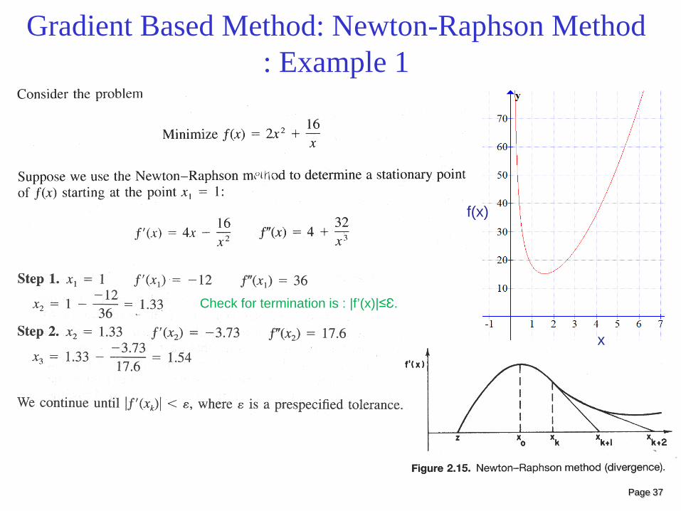
Gradient Based Method: Newton-Raphson Method : Example 1

Check for termination is : |f’(x)|≤Ɛ.

f(x)

x

Page 38

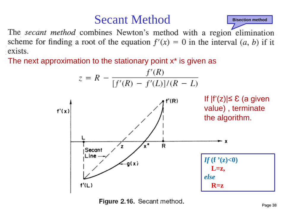
Secant Method

The next approximation to the stationary point x* is given as

If |f’(z)|≤ Ɛ (a given value) , terminate the algorithm.

Bisection method

If (f ’(z)<0) L=z, else R=z

Page 39

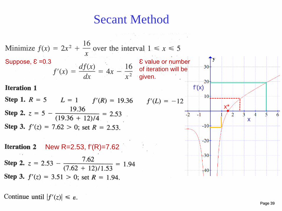
Secant Method

New R=2.53, f’(R)=7.62

Ɛ value or number of iteration will be given.

f’(x)

x

x*

Suppose, Ɛ =0.3

Page 40

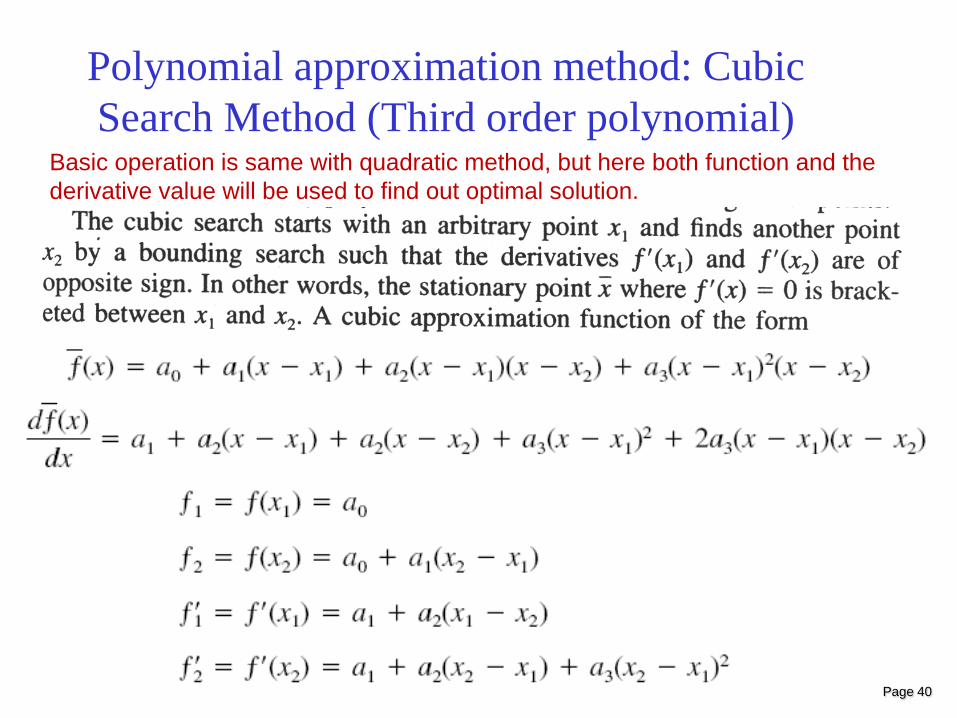
Polynomial approximation method: Cubic Search Method (Third order polynomial)

Basic operation is same with quadratic method, but here both function and the derivative value will be used to find out optimal solution.

Page 41

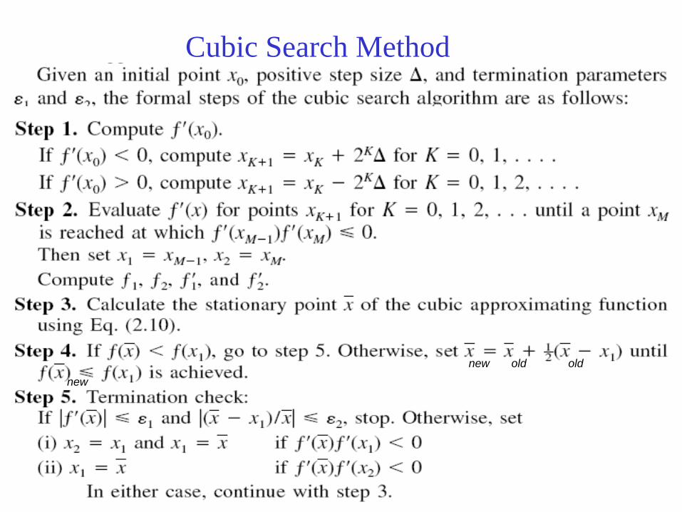
Cubic Search Method

old old new new

Page 42

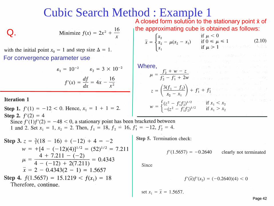
Cubic Search Method : Example 1

For convergence parameter use Where,

Q. A closed form solution to the stationary point ẋ of the approximating cube is obtained as follows:

Page 43

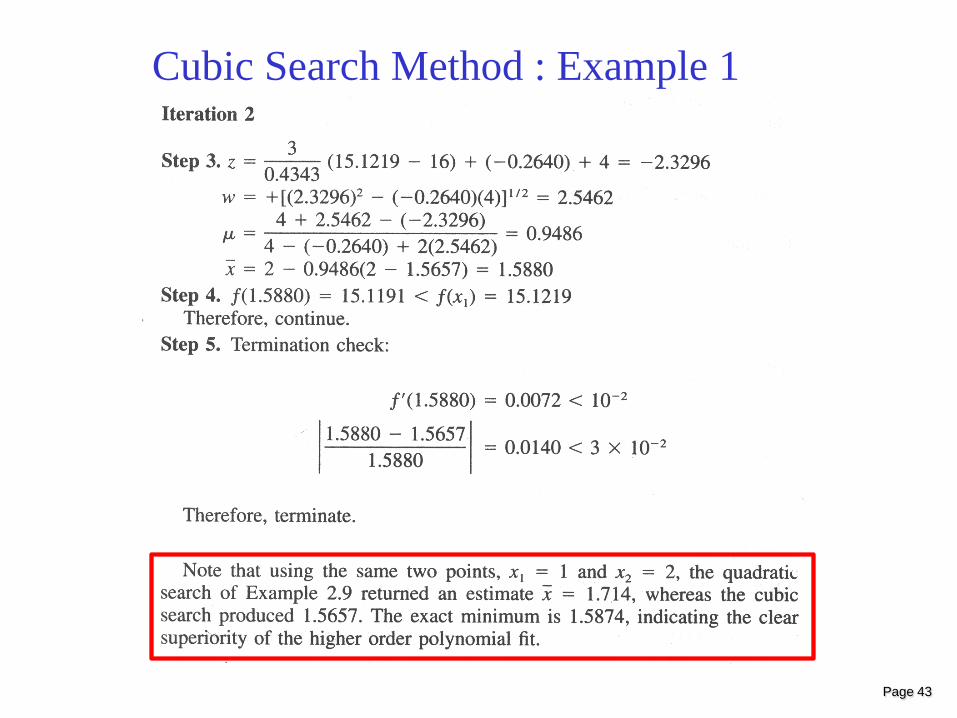
Cubic Search Method : Example 1

Page 44

References

1. Optimization for Engineering Design by Kalyanmoy Deb

2. Engineering Optimization: Methods and Applications by A.

Ravindran, K, M, Ragsdell, G.V. Reklaitis

3. Engineering Optimization: Theory and Practice by S. S. Rao