Ajay Dashora* Bharat Lohani Kalyanmoy Deb Procedure_IJMMNO_2013.pdf · scanning angle, scanning frequency and point repetition frequency) impose the ... method and also describe two-step

Int. J. Mathematical Modelling and Numerical Optimisation, Vol. X, No. Y, xxxx 1

Copyright © 200x Inderscience Enterprises Ltd.

Two-step procedure of optimisation for flight planning problem for airborne LiDAR data acquisition

Ajay Dashora* Department of Civil Engineering, Indian Institute of Technology Kanpur, Kanpur, 208016, India E-mail: [email protected] E-mail: [email protected] *Corresponding author

Bharat Lohani Department of Civil Engineering, Indian Institute of Technology Kanpur, Kanpur, 208016, India E-mail: [email protected]

Kalyanmoy Deb Department of Electrical and Computer Engineering, Michigan State University, 428 S. Shaw Lane, 2120 EB East Lansing, MI 48824, USA Fax: 517-353-1980 E-mail: [email protected]

Abstract: Flight planning for airborne LiDAR data collection determines flight parameters, which in turn control the flight duration. While the former ensures desired quality of captured data the cost of the project is directly affected by the latter. This paper attempts to optimise flight planning problem. The flight duration is expressed as an objective function and the associated data requirements, preferences and limitations of flight planning problem are considered as constraints. Due to the typical characteristics of flight duration and flight parameters, a two-step procedure of optimisation that consists of genetic algorithms (GA) and Hooke and Jeeve’s (HJ) method of optimisation are adopted. The two-step procedure alleviates the pitfalls of both GA and HJ method and successfully determines the optimal flight planning parameters for a fairly complicated problem. Results obtained in this paper demonstrate that the proposed two-step procedure can be used for solving complex engineering problems like flight planning.

Keywords: two-step procedure; optimisation; flight planning; airborne LiDAR data acquisition; genetic algorithms.

2 A. Dashora et al.

Reference to this paper should be made as follows: Dashora, A., Lohani, B. and Deb, K. (xxxx) ‘Two-step procedure of optimisation for flight planning problem for airborne LiDAR data acquisition’, Int. J. Mathematical Modelling and Numerical Optimisation, Vol. X, No. Y, pp.000–000.

Biographical notes: Ajay Dashora received his MTech and PhD degree in geoinformatics specialisation from Department of Civil Engineering, Indian Institute of Technology Kanpur, India, respectively, in years 2005 and 2013. His PhD thesis problem was addressing the problem of development of optimisation system for airborne LiDAR data acquisition. His research interests include physical modelling, use of evolutionary algorithms in remote sensing, integration of airborne data acquisition methods and techniques, application of remote sensing techniques, use of evolutionary algorithms in remote sensing, compatibility studies, and synthetic simulation.

Bharat Lohani is an Associate Professor at Indian Institute of Technology Kanpur, India. He has interest in teaching and research in the domain of laser scanning-data capture, processing and application development.

Kalyanmoy Deb is the Koenig Endowed Chair Professor at Electrical and Computer Engineering in Michigan State University, USA. His research interests are in evolutionary optimisation and their application in optimisation, modeling, and machine learning. He was awarded ‘Infosys Prize’, ‘TWAS Prize’ in Engineering Sciences, ‘CajAstur Mamdani Prize’, ‘Distinguished Alumni Award’ from IIT Kharagpur, ‘Edgeworth-Pareto’ award, and Bhatnagar Prize in Engineering Sciences. He is a Fellow of IEEE and three science academies in India. He has published 350+ research papers with Google Scholar citation of 54,000+ with h-index 77. He is in the editorial board on 18 major international journals.

1 Introduction to flight planning problem for ALS

Airborne LiDAR scanning (ALS) provides 3D topographic data of a terrain surface with certain attributes like planimetric (horizontal) and altimetric (vertical) accuracies, data density, overlap, etc. Due to negligible dependencies on the accessibility and type of terrain conditions (rough and undulating, plane or steep), the ALS is considered to be a viable option for capturing highly accurate 3D topographic data. As a result, the ALS is being used for different types of applications: forest management, mining, oil and gas explorations, corridor mapping, environmental monitoring, utility surveillance and management, engineering and construction, municipal mapping, real estate development, flood plain mapping, etc. (DWMI, 2007). However, the cost involved is higher due to the expensive hardware and complicated operations. Flying for data capture is one such complicated operation which directly controls the cost of the project.

Flying operations, apart from the other critical operations, consists of flying the aircraft (or helicopter) in stable position (ideally no change or vibrations in attitude and altitude with respect to time) over the given area of interest (AOI) on terrain. Moreover, in addition to the flying direction and flying height, other parameters (aircraft speed, scanning angle, scanning frequency and point repetition frequency) impose the constraints on the flight duration. Therefore, it should maintain a known direction of flight and height. The problem of altitude and attitude measurement is alleviated

Two-step procedure of optimisation for flight planning problem 3

as inertial measurement unit (IMU) and global positioning system (GPS), which respectively determine attitude (roll, pitch, yaw angles) and the position (3D coordinates of aircraft trajectory) of an aircraft with considerable accuracy and precision are integrated with LiDAR scanner onboard. However, the quality of the data gathered depends on the flight parameters and the nature of ground, where the former include the parameters of sensor and aerial platform. Moreover, the cost of flying operation is directly dictated by the duration of the flight. Therefore, aerial LiDAR data acquisition demands optimum flying parameters that minimise the flight duration while at the same time ensure the quality and quantity of data.

This paper first addresses the flight planning problem in detail, formulates the objective function, identifies the parameters of flight planning, explains the derived methodology to obtain the optimum result, and performs the minimisation of the flight duration. The basic details of ALS are given in Baltsavias (1999) and Wehr and Lohr (1999). The definitions of fundamental terms (scanning angle ‘φ‘, scanning frequency ‘f’, flying height ‘H’, flying speed ‘V’, point repetition frequency or PRF ‘F’) and the derived terms (effective swath ‘B’, point density or data density ‘ρ’, along track spacing ‘DA’, across track spacing ‘DS’) related to laser scanning are adopted from Baltsavias (1999) and Wohr and Lohr (1999). The formulations of turning time involved in the objective function are not derived here but are done in the technical report describing the turning time calculations (Dashora and Lohani, 2013a). Furthermore, planimetric and altimetric errors of 3D data can be found in technical report of error calculation for airborne LiDAR data (Dashora and Lohani, 2013b).

The paper is organised in ten sections. Introduction to flight planning problem in Section 1 is followed by the detailed description of problem with technicalities in Section 2. Section 3 formulates the flight planning problem as optimisation problem and defines the objective function and constraints. Sections 4 and 5 select the optimisation method and also describe two-step procedure of optimisation. Sections 6 and 7 perform the optimisation for flight planning problems, respectively, for simulated and real test sites. Section 8 presents the flight plans for the two AOIs. Section 9 provides a guideline on minimum number of simulations to be performed for obtaining the results with higher confidence. Conclusion is presented in Section 10.

2 Description of flight planning problem for ALS

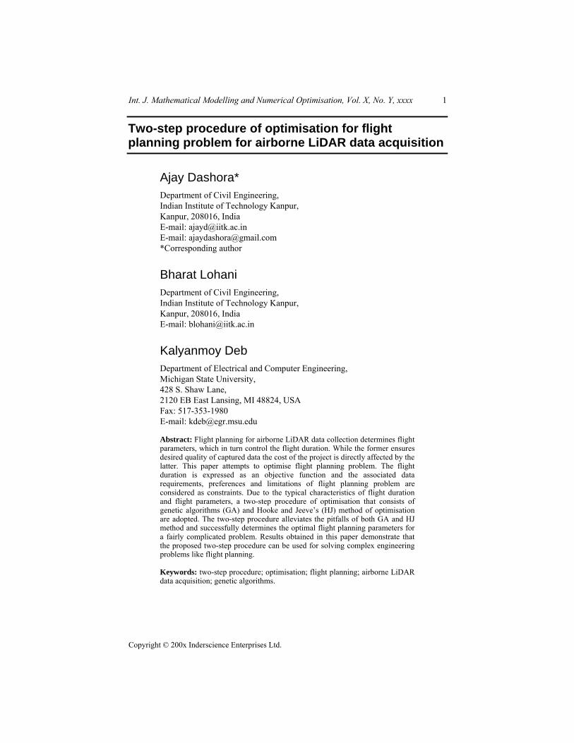
ALS operation consists of scanning over the ground using a LiDAR scanner, mounted in an aircraft or helicopter, and thus measuring the range (direct distance from laser emitter to the ground) to a ground point. In order to measure the range of the point, LiDAR scanner fires a laser pulse that reaches the ground by travelling through the atmosphere with the velocity of light and reflects back from the ground to be captured by the scanner’s receiver. The time difference between the firing and receiving of the laser pulse gives a measure of the distance or range. As mentioned earlier, LiDAR scanner is integrated with the GPS and IMU devices that provide 3D coordinates in WGS84 reference system (Hofton et al., 2000). The 3D coordinates of the collected data points on the ground surface collectively represent the terrain. Although, the laser pulses are fired with regular time interval to form a scanning pattern, data points on the surface of ground are collected in a pseudo-random manner. As an example the process of data collection using the ALS is illustrated in Figure 1.

4 A. Dashora et al.

Figure 1 Airborne LiDAR scanning process (see online version for colours)

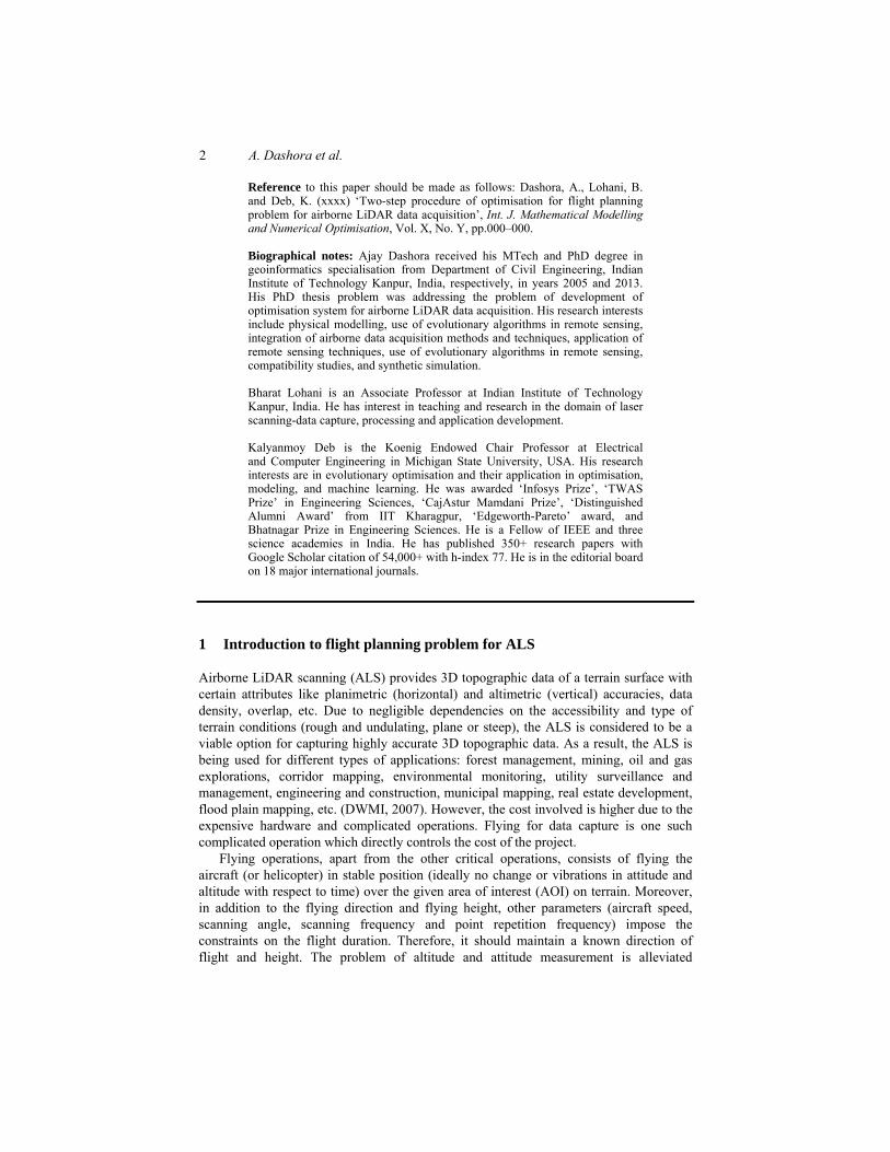
During the scanning process, the pulses are fired successively in the field of view (FOV). The FOV is equally divided on both sides (left and right) with respect to the nadir direction at the emitter. The half of the FOV is termed as ‘half scan angle’ and denoted by φ. The angle φ of a scanner mounted in an aircraft, which is flying at a height H with reference to a datum, forms ‘swath’ (Bs) or width of a flight strip on the ground (Figure 2) and is expressed as:

2 tan( )sB H= φ (1)

Figure 2 Schematic view of half scan angle, flying height, swath, Z shape scanning pattern, along track spacing, and across track spacing for ALS

Ideally, the swath is equal to the spacing between the centre lines of two adjacent flight strips which have no overlap. However, due to the overlap, which is maintained between two adjacent flight strips for continuity of data and error removal (Bang et al., 2009), the distance between the flight lines or centre lines of flight strips is reduced to the ‘effective swath’. The effective swath (B) is written as:


(1 )sB B P= − (2)

where P is ‘percentage overlap’ (Shih and Huang, 2009) or ‘overlap fraction’ that represents the fraction (or percentage) of the swath which lies under the area of overlap at the edges of two adjacent flight strips on the map.

‘Speed’ (V) of an aircraft along the flight direction realises the second dimension of scanning process as an aircraft moves by a distance equal to the speed in one second (Wehr and Lohr, 1999). Due to the movement in flying direction, the scanning lines, which are obtained across flying direction, appear in a Z shape, which is termed as saw tooth or zigzag pattern (Baltsavias, 1999). As shown in Figure 2, all scanning lines, which are formed by movement of oscillating mirror in one direction (left to right or right to left) are parallel to each other, however, none of these are exactly perpendicular to the flying direction. Figure 2 is an exaggerated view of the actual scanning mechanism. In reality, the across track spacing (DS) between two successive points in a scan line is not uniform and is minimum at the centre and maximum at the ends.

Apart from the Z shaped pattern, it is possible to generate many more patterns (Jenkins, 2006) by different type of sensors (Baltsavias, 1999); this study is performed using Optech’s airborne LiDAR scanner model ‘ALTM 3100EA’ which creates bidirectional Z shape (zigzag) pattern. The characteristics and criticality of the relevant parameters of ‘ALTM 3100EA’ model are discussed in Section 5.

An aircraft, after covering one flight strip, navigates back to the starting point of the next parallel strip through a 180° level turn or horizontal course reversal. For any strip, which is essentially not the first strip, aircraft navigates in opposite direction than that of the last strip and thus covers the complete AOI in finite number of strips. Turning from one flight line to the next flight line can be performed by consecutive turning, non-consecutive turning, or hybrid turning (Dashora and Lohani, 2013a).

As stated earlier, flying operations are the most critical part of airborne data collection as during this period, the required quality of data is ensured by adopting the appropriate flight planning parameters. Moreover, it takes considerable resources amongst all project operations. Furthermore, flying an aircraft includes expensive logistics requirements, severe risks and consequently accounts for higher cost. Apart from that, unlike conventional topographic survey practices performed on ground, airborne survey cannot be repeated without a justified reason due to intricacies and cost involved. Therefore, minimising the duration of flight is the only desirable solution for exploiting the real potential of the airborne surveys. The next section presents the expression of flight duration with minimum derivations and analysis and then leads to the constraints imposed due to the LiDAR survey requirements.

3 Objective function and constraints

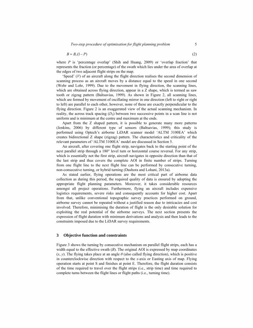
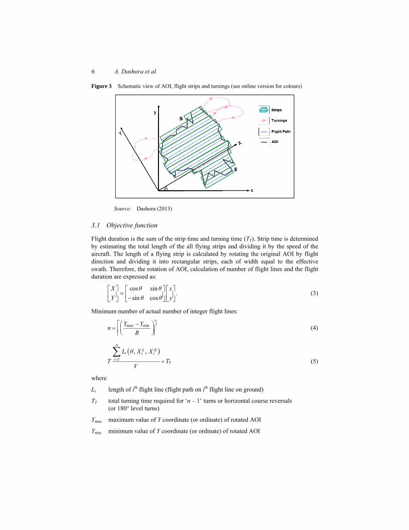
Figure 3 shows the turning by consecutive mechanism on parallel flight strips, each has a width equal to the effective swath (B). The original AOI is expressed by map coordinates (x, y). The flying takes place at an angle θ (also called flying direction), which is positive in counterclockwise direction with respect to the x-axis or Easting axis of map. Flying operation starts at point S and finishes at point E. Therefore, the flight duration consists of the time required to travel over the flight strips (i.e., strip time) and time required to complete turns between the flight lines or flight paths (i.e., turning time).

6 A. Dashora et al.

Figure 3 Schematic view of AOI, flight strips and turnings (see online version for colours)

Source: Dashora (2013)

3.1 Objective function

Flight duration is the sum of the strip time and turning time (TT). Strip time is determined by estimating the total length of the all flying strips and dividing it by the speed of the aircraft. The length of a flying strip is calculated by rotating the original AOI by flight direction and dividing it into rectangular strips, each of width equal to the effective swath. Therefore, the rotation of AOI, calculation of number of flight lines and the flight duration are expressed as:

cos sin.

sin cosX θ θ xY θ θ y⎡ ⎤ ⎡ ⎤ ⎡ ⎤

=⎢ ⎥ ⎢ ⎥ ⎢ ⎥−⎣ ⎦ ⎣ ⎦ ⎣ ⎦ (3)

Minimum number of actual number of integer flight lines:

max minY YnB

⎡ − ⎤⎛ ⎞= ⎜ ⎟⎢ ⎥⎝ ⎠⎢ ⎥ (4)

( )1

, ,n

L Ri i i

iT

L θ X XT T

V= +∑

(5)

where

Li length of ith flight line (flight path on ith flight line on ground)

TT total turning time required for ‘n – 1’ turns or horizontal course reversals (or 180° level turns)

Ymax maximum value of Y coordinate (or ordinate) of rotated AOI

Ymin minimum value of Y coordinate (or ordinate) of rotated AOI


LiX value of X coordinate of left edge (or left end) of ith flight strip (or flight line) in

rotated AOI RiX value of X coordinate of right edge (or left end) of ith flight strip (or flight line) in

rotated AOI.

The length and location of centre line of the ith strip and the corresponding length of turning for given θ, are dictated by the size of the effective swath (B) as it affects the number of strips [equation (4)]. Unlike the formulation for strip time as shown above, the derivation of relationship for turning time is complex and cumbersome. Therefore, for the conciseness of the discussion, the formulation and algorithm to determine the turning time is adopted from the technical report of turning time calculation (Dashora and Lohani, 2013a). Details of the algorithms for calculating the turning time are presented in appendix.

3.2 Constraints

The data captured by the ALS should fulfil certain qualities. In this paper, constraints related to the data density, overlap, spacing of data points in along track and across track directions, errors in data, simultaneous photographic data acquisition, scanner product, and safety regulations are considered and mentioned in the discussion below.

1 Minimum and maximum data density: It is evident from the explanation of ALS mechanism that in one second duration a scanner effectively covers an area equal to the product of effective swath and speed (BV). Furthermore, during the same time period, it fires and collects the 3D information for F number of pulses. Therefore, the ‘data density (ρ)’ (also known as ‘point density’) can be written as:

.FρBV

⎛ ⎞= ⎜ ⎟⎝ ⎠

(6)

The density of data collected, however, should be in the range of minimum data density (ρL) and maximum data density (ρU), which are specified by a user. Therefore, the constraints on data density are written as:

.L Uρ ρ ρ≤ ≤ (7)

Tolerance in data density (τ max) connects the maximum and minimum data density by following relationship (Dashora, 2013):

( )max1 .U Lρ ρ τ= + (8)

2 Minimum overlap: Mapping agencies like United States Geological Survey (USGS, 2010) recommends a minimum of 10% overlap on all parts of terrain surface. As a result, at no part of terrain the overlap should be lesser than the minimum overlap (Pmin), which is, therefore, the limiting overlap at the highest point of terrain. A maximum overlap (Pmax) may also be specified which will be limiting overlap at the lowest elevation of terrain. Contrary to overlap, the data density reaches its maximum and minimum values at the highest and lowest points of terrain, respectively. Dashora (2013) provides an algorithm that considers theoretical

8 A. Dashora et al.

relationships between the data density (ρ), overlap (P), terrain elevation (dt), and flying height (H). According to the algorithm, instead of bounding the data density (ρ) by its upper bound value (ρU), the tolerance in data density (τρ) is restricted by a maximum value (τmax). The algorithm is given in the form of pseudo code as: a given: 3D information of terrain (dt) with known accuracy

• tolerance in data density (τρ) constrained in a range from τmin to τmax b select: flying height (H) and half scan angle (φ) c calculate: relief ratio PR = dt / H

• tolerance in data density τρ ≥ PR / (1 – PR) • maximum overlap fraction at datum P = 1 – (1 – PR) (1 – Pmin) • swath at datum Bs = 2Htanφ • effective swath B = (1 – P)Bs

d check the constraint: calculated τρ should be in the range specified (τmin to τmax) • termination: if constraint is not satisfied, repeat with different values of

flying height (H) and half scan angle (φ).

3 Spacing of data points: Equation (6) is a general equation representing data density independently of the type of scanning pattern, as it is a function of area covered in unit time (one second duration). However, within this area (BV), the uniformity of the 3D data is dictated by the spacing between the successive and similar points in longitudinal (along-track) and lateral direction (across-track), respectively. In order to achieve uniformity in spread of data points (to avoid data clustering), the across track spacing and along track spacing should be of comparable magnitude (USGS, 2010). Therefore, the ratio of absolute difference between the along track spacing (DA) and across track spacing (DS) to the along track spacing (DA) should be less than or equal to some user defined threshold on spacing (εd). Accordingly, the constraint on the spacing of the LiDAR data points is written in a generic form as:

.A Sd

A

D D εD−

≤ (9)

The spacing in the along track and across track directions can be considered by many criterions like average, maximum or minimum. For Z shape pattern of scan lines, the average values of along track spacing and across track spacing are calculated as (Baltsavias, 1999):

2AVD

f⎛ ⎞= ⎜ ⎟⎝ ⎠

(10)

2 .sS

fBDF

= (11)

4 Planimetric and altimetric errors in data: The planimetric and altimetric errors in LiDAR data are restricted by maximum allowable values of respective errors, which are decided by a user as per the application. The calculation of the errors for the LiDAR data involves propagation of random errors in various measurements by


scanner, IMU, GPS, and spatial arrangement between these measuring units. The procedure of calculation is adopted from the error calculation report (Dashora and Lohani, 2013b).

p Hσ e≤ (12)

v Vσ e≤ (13)

where

2 2p pP X Yσ σ σ= + (14)

pv Zσ σ= (15)

pXσ 1σ error in x-direction of local tangent plane at a point

pYσ 1σ error in y-direction of local tangent plane at a point

pZσ 1σ error in z-direction perpendicular to local tangent plane at a point

eH maximum allowable 1σ planimetric error (or horizontal) in local tangent plane at a point

eV maximum allowable 1σ altimetric (or vertical) error in local tangent plane at a point.

5 Scanner product: This category of constraints includes all constraints, which are imposed by the physical limitations of LiDAR or other scanners mentioned by the scanner manufacturer. For example, in case of ALTM3100EA scanner instrument, the scanner product is given by:

1,000.f ≤φ (16)

6 Safety regulations: Amongst all safety regulations, the minimum eye safe distance (ESD) for the laser pulse, and minimum flying height or Hmin (according to air traffic control or ATC standards) are considered. Maximum of the eye safe distance (ESD) and minimum flying height (Hmin) should be added to maximum elevation of terrain (hmax) and the flying height (H) should be more than the calculated distance values as:

( )( )max minmax , .H h H ESD≥ + (17)

ESD depends upon the LiDAR scanner and generally mentioned by the manufactures. However, for India, a minimum of 305 metres (1,000 feet) flying height is recommended (DGCA, 2010).

7 Simultaneous photographic data acquisition: According to recent practice, along with LiDAR data, photographic or image data are also captured using airborne digital camera (Landtwing and Whitcare, 2008). As flight planning process is optimised for the LiDAR data acquisition, the photographic data capture is accommodated with additional constraints. Following four requirements are framed as constraints (Dashora, 2013):

10 A. Dashora et al.

a Camera and LiDAR sensor selection: Dashora (2013) derived a relationship for calculating the maximum half scan angle (φMax) of LiDAR sensor that restricts the value of half scan angle, for the given FOV of camera (φopt). It should be noted that half scan angle, can be programmed by a flight planner before data acquisition. Consequently, the FOV of LiDAR scanner, which is equal to twice of the half scan angle, is decided by the flight planner for LiDAR scanner. The relationship, which ensures the minimum side lap of images captured by camera and minimum strip overlap of LiDAR data, is given by (Dashora, 2013):

1 1tan tan .

1 2ecy opt

Maxe

PP

− ⎛ − ⎞⎛ ⎞ ⎛ ⎞≤ ⎜ ⎟⎜ ⎟⎜ ⎟− ⎝ ⎠⎝ ⎠⎝ ⎠

φφ (18)

For a camera of 44° FOV, equation (18) calculates the maximum half scan angle value equal to 18.6°. However, if a camera (camera come with fixed FOV) is selected during the flight planning; it allows the calculation of maximum half scan angle of the LiDAR scanner. Consequently, after calculating the maximum half scan angle value for LiDAR scanner, this constraint is not needed to be considered in the solution process as henceforth the maximum half scan angle can be considered as the computed one or as the one recommended by the USGS (i.e., 20°).

b Ground sampling distance (GSD): GSD of captured image should be less than or equal to the user defined value of maximum GSD (GSDMax). Therefore,

.MaxGSD GSD≤ (19)

c Exposure interval: The photographs on a flight line are captured by successive exposures of camera. The time period between the two successive exposures of camera is termed as ‘exposure interval’ (Grendzdörffer, 2008). Therefore, the distance travelled by an aircraft during the exposure interval (in seconds) between two successive exposures of a camera should be more than the length of the area captured by a pair of stereo images along the flight direction. The resulting inequality relationship is (Grendzdörffer, 2008):

( )1 cx pxei

GSD P nt

V⎛ ⎞−

≤ ⎜ ⎟⎝ ⎠

(20)

( )1 .cx ecx ecx RP P P P= + − (21)

d Horizontal accuracy of orthoimage: A digital map (or orthoimage) is prepared from the captured images. For the desired GSD of orthoimage (ortho GSD), GSD of image should be constrained by the following empirical relationship (Dashora, 2013):

(0.884) orthoGSD GSD≤ (22)

where

p

c

HsGSD

f⎛ ⎞= ⎜ ⎟⎝ ⎠

(23)

sp size of a pixel of airborne digital camera


fc focal length of camera npx number of pixels in camera in along track direction φMax maximum allowable value of half scan angle φopt camera FOV Pcx endlap (or overlap in along track dierction) between two consecutive

images at datum Pecx minimum endlap (or overlap in along-track direction) between two

consecutive images (RICS, 2010) Pecy minimum sidelap (or overlap in across-track direction) between two

consecutive images (RICS, 2010) Pe minimum overlap (in across-track direction) between two adjacent strips

of LiDAR data.

4 Constrained minimisation of flight duration

4.1 Identification of design variables of flight planning problem

It is evident from the expressions of objective function [equations (3) to (6)], that for given AOI, data specifications and other environmental variables, the flight duration is a function of half scan angle (φ), flying height (H), speed of aircraft (V), and flying direction (θ). However, the constraints, in addition to these four variables, are also dictated by the scanning frequency (f), and PRF (F). Therefore, there are six variables that influence the minimisation of flight duration under constraints. The remaining variables are either characteristics of sensors (LiDAR scanner, camera, GPS, IMU) or environmental variables. Environmental variables, which represent the user defined requirements of data or user defined preference for flying operations (i.e., maximum bank angle, or cushion period), remain constant for a given problem of flight planning. Values of environmental variables are shown in Table 1. The next section discusses about the characteristics of sensors used in this study. Table 1 Data requirements in optimisation problem

Parameter Symbol Value Minimum data density ρL 11 points/m2 Maximum data density ρU 13 points/m2 Maximum tolerance in data density τmax 30% Tolerance of spacing constraint εd 10% Minimum overlap Pe 10% Maximum altemetric error eV 0.10 m Maximum planimetric error eH 0.15 m Maximum GSD GSDMax 0.15 m Minimum endlap Pecx 60% Minimum sidelap Pecy 25% Maximum bank angle βmax 25º Cushion period tC 30 seconds


4.2 Characteristics of sensors (GPS, IMU, LiDAR scanner, camera)

The selection of a suitable and appropriate optimisation scheme for flight duration minimisation requires a comprehensive understanding of the characteristics of the variables involved and their observation by the sensors. Information about the navigation sensors (IMU and GPS units) is important for evaluation and control of the error. Further, the spatial interrelationship between the LiDAR scanner and IMU unit should also be known. Therefore, it is assumed that the latest calibration reports of all sensors are available. The values of precision parameters are selected from the paper by Glennie (2007) for the calculation of the propagated errors in the LiDAR data (Dashora and Lohani, 2013b). Details of the error calculation are beyond the scope of this paper. However, it should be noted that the flying height (H) and half scan angle (φ), which are decision variables in optimisation process, participate in the error calculation. ALTM3100 EA LiDAR scanner, which is manufactured by Optech Inc., is used in this study. Similarly, Applanix DSS 322, which is a medium format digital airborne camera, is selected. Following Tables 2 and 3 show the salient and relevant features of ALTM3100 EA scanner and Applanix DSS 322 camera. Table 2 Specifications of ‘ALTM 3100EA’ LiDAR scanner

Values Parameter

Range Least count

Flying height (H) 80–3,500 m Continuous Scanning frequency (f) 1–70 Hz 1 Hz

Scanning angle (φ) 1–25° 1°

PRF (F) {33, 50, 70, 100} kHz (if 80 ≤ H ≤ 1,100 m) {33, 50, 70} kHz (if 1,100 < H ≤ 1,700 m) {33, 50} kHz (if 1,700 < H ≤ 2,500 m) {33} kHz (if 2,500 < H ≤ 3,500 m)

Source: Optech (2006a)

Table 3 Specifications of ‘Applanix DSS 322’ camera scanner

Parameter Value

Pixel size (sp) 9 microns Number of pixels along-track (npx) 4,092 Number of pixels across-track (npy) 5,436 Focal length (fc) 60 mm

FOV across-track (φc) 44°

Exposure time* (tet) 1/125–1/4,000 seconds Exposure interval (tei) 2.5 seconds

Note: *Slower shutter speed (higher exposure time) not recommended. Source: Optech (2006b)

The speed of an aircraft for airborne LiDAR data acquisition can vary in a large range, i.e., 10–140 knots (5.14 to 72 m/s) (Saylam, 2009). Specific to the ALTM 3100EA scanner, latest practices prefer Cessna aircraft or helicopter. The recommended range of


speed of an aircraft (aircraft and helicopter) and the least count of scanning frequency and scanning angle are obtained by private communications with Mariusz Boba and Jake Carroll.

4.3 Selection of optimisation method for minimisation problem

Amongst the six variables of design vector of optimisation, three variables namely the half scan angle (φ), scanning frequency (f) and PRF (F) are the features of a LiDAR scanner and thus these are addressed as scanner parameters. The remaining three variables (flying height, flying speed and flying direction) are related to flying operation and therefore, these are termed as the flying parameters. The salient characteristics of the scanning parameters, flying parameters, flight duration and constraints are as following:

1 Scanner parameters are discrete parameters. More specifically, the PRF is a discontinuous parameter which is decided according to the flying height. However, flying parameters are continuous parameters. Therefore, the objective function (flight duration) and constraints are function of discrete as well as continuous variables.

2 Flight duration is a sum of the strip time and turning time. The strip time is the summation of the time taken to cover individual strips of varying length. For an arbitrary shaped AOI, the strip time is discontinuous mathematical functions. Moreover, on the other hand, the turning time is a function of the flying speed and maximum banking angle. During flying operations, the maximum banking angle remains constant in practice. The flying speed is a continuous variable. As an aircraft has to turn to one of the flight lines which are finite in number, are regularly spaced and have pre-decided locations, the turning mechanism (consecutive, non-consecutive or hybrid turnings) makes the flight duration discontinuous. Switching between the parallel flight lines for covering all flight lines in minimum time is equivalent to the problem of travelling on parallel edges and shifting from one edge to the other in minimum time. The problem of travelling on parallel edges and switching between these is non-solvable in polynomial time using classical combinatorial optimisation techniques (Benavent et al., 2005).

3 The scanner and flying parameters appear as non-separable variables in the expressions of flight duration and constraints, where the latter are implicit non-linear mathematical functions.

4 The error in 3D coordinates has an inverse relation with the fight duration with respect to the changes in flying height and scan angle (i.e., with the increase in flying height and scan angle the flight duration will decrease but the errors increase, and vice versa.

As per the characteristics of variables, applicable constraints and the objective function discussed above, the problem of optimisation in the current case is a mixed integer non-linear problem (MINLP). However, the non-linear implicit equations of mathematically discontinuous objective function and constraints, which are defined in terms of discrete and continuous variables, limit the use of conventional (classical) optimisation methods. Additionally, the existence of derivatives and unimodal property of objective function is also not guaranteed in such problems. In view of the non-linear


single-objective constrained optimisation problem with discontinuous objective function and constraints, which are defined in terms of non-separable discrete and continuous variables, the evolutionary algorithms can be found useful.

Recently, Rodrigues and Ferreira (2012) combined the GA and local search method for solving the shortest path of travel on edges (or rural postman problems). Moreover, the exploration and development of GA in the last two decades at the Kanpur Genetic Algorithm Laboratory (KanGAL) in IIT Kanpur is a strong motivational reason to use it as a tool for optimisation of complex flight planning problem. Furthermore, the real-coded genetic algorithms (RGA) code is available online at KanGAL’s website for solving the single objective optimisation problem. However, in spite of their revolutionising development and implementation for real life applications at KanGAL and world over in the last few years, these are not yet explored for flight planning and flight duration constrained minimisation problem. Furthermore, for non-linear functions, a classical method demands an initial point or solution of design variables which should be in the vicinity of the desired optima.

On the other hand, a general notion is that an optimisation problem may take significantly longer time for convergence. Moreover, for convergence to the global optima, the time required by GA of infinite scale cannot be accommodated in practical sense. Conversely, the potential of the classical methods for fast convergence, due to their intelligent search procedure in a local neighbourhood of initial point, cannot be ignored. Therefore, it is wise to use a hybrid algorithm that utilises the potentials of both classical and evolutionary methods and in turn compensates for the pitfalls of both sides. There are a number of classical methods available in the literature with different applicability. However, as explained in the previous section, the flying speed and various turning mechanisms performed on finite number of flight lines makes the flight duration a discontinuous function. A slight variation in flying speed may change the turning mechanism from one type to another type. Therefore, a classical method which does not require assumptions of continuity and existence of the derivatives of the objective function is desired. Fernandes et al. (2011) and Costa et al. (2012) presented hybrid optimisation algorithms that combine GA and various classical methods. Fernandes et al. (2011) combined the branch and bound (B&B) method with GA to solve the MINLP problem. The study by Costa et al. (2012) devised Hybrid Genetic Pattern Search Augmented Lagrangian (HGPSAL) algorithm by integrating the GA with Hooke and Jeeve’s (HJ) method, which is a derivative free pattern search method, and constraints are handled by the augmented Lagrangian method. Considering the nature of the objective function of flight planning problem, hybrid approach of two-step procedure using the HJ method and GA is proposed for the flight planning problem in this study. Next section explains the GA and HJ method briefly. As the proposed method is not ever implemented and tested for the flight planning problem, a simulation study is conducted for the flight planning problem which is presented in the subsequent section and later the proposed approach is applied on the flight planning problem on an actual test site with defined data requirements.


5 Two-step procedure of optimisation

5.1 Introduction to genetic algorithms

Genetic algorithms (GA) are amongst the most popular evolutionary methods. GA are advanced statistical methods that are independent of the initial estimates of parameters. Furthermore, these are not limited by the restrictive assumptions like unimodality, continuity of design variables (parameters), objective functions (or fitness function), constraints, and the existence of derivatives of objective functions or constraints (Goldberg, 1989).

The search procedures in GA start with the multiple numbers of the trial values of parameter vectors (also known as population of design vector or parameter vector), in contrast to the conventional optimisation technique which begins with a single initial value of the design vector. The value of objective function is utilised to generate a population for the next search using the probability transition rules instead of the derivatives, auxiliary knowledge, or deterministic rules. A simple GA that yields good result is usually composed of three operators: reproduction, crossover, and mutation. Reproduction is a process in which the individual trial design vectors (vector of design variables) are selected to participate in the next generation of offspring as parents, according to their objective function values. In a minimisation problem, the design vectors with a lower value of objective function have a higher probability of contributing towards the production of offspring in the next generation. Crossover follows the reproduction and proceeds in two steps. First, the members of newly produced vectors are mated at random and secondly each pair of design vector undergoes crossing over by random swapping. Although the reproduction and crossover efficiently search and recombine good extant notions, occasionally they may also lose some potential genetic material. Such irrecoverable loss is protected by mutation. Mutation is occasional random alteration of the value of a parameter in a design vector (Goldberg, 1989).

5.2 HJ method

Explanation and implementation of HJ method is adopted from Kaupe (1963). After explanation of the method in a generic sense in the forthcoming discussion, it is modified for the flight planning problem with flying height (H), flying direction (θ) and the flying speed (V) as variables.

For HJ method, the initial point or guess (p0), which is an estimate of the optimal solution in multidimensional parameter space, is a prerequisite. Moreover, for the first iteration, a step length (Δ1) for each dimension (or variable) of optimisation problem is predefined. The HJ method performs optimisation as explained in the following steps:

1 At the start of the optimisation process, the given initial point or guess (p0) is considered as the current position for the first iteration. In the process of optimisation, in the kth iteration, the current position and step length are denoted by pk–1 and Δk, respectively.

2 The HJ method, in the kth iteration, explores the parameter space by shifting the current position (pk–1) by a step length (Δk) along a variable’s coordinate axis in both negative and positive directions. At the shifted positions, the objective function values are evaluated. If a shift by step length gives a superior result of objective


function, the current position (pk–1) is updated by step length to occupy the new position (pk). This process is repeated for all direction axes.

3 In Step 2, if improvement in objective function value is recorded, Step 2 is repeated for the next iteration with the same step length.

4 In case of no improvement or inferior result, the current position is not updated (or current position itself becomes new position for the next iteration). The HJ method, at this stage, reduces the step length (Δk = pk – pk–1) of kth iteration by a predefined factor (rHJ) to calculate the step length of the next iteration. The factor (rHJ) used for reduction of step length should be close and lesser than one for exhaustive exploration and smooth transitioning through the parameter space.

5 The above three steps are repeated in succession till an improvement in the value of the objective function is found below a certain threshold. Moreover, the algorithm is also terminated intermediately if the maximum allowable number of iterations is reached.

For the flight duration minimisation, the step length vectors (Δ1) for three variables are calculated by dividing the range of individual variables by the population size. The following sections implement the suggested two-step procedure for the simulated AOI in sequential manner, i.e., the results obtained by GA are refined by HJ method which is a classical pattern search method. The algorithm of the two-step procedure, which is precisely used in this paper, is shown below by pseudo code.

5.3 Pseudo code of two-step procedure of optimisation

5.3.1 First step: optimisation by GA

1 Initialisation • define the population count (number of samples) and number of maximum

generations • initialise the population.

2 Regeneration a fitness function and constraint evaluation: calculate the values of objective

function and constraints b selection and generation of population:

• using the values of fitness function and constraints, rank the individual sample of population

• form a new population by the cross-over, mutation, and elite preservation on population samples of current generation

c generation counter: count the number of generation.

3 Termination of GA • if the number of generations is equal to the maximum generation, terminate the

GA and accept the current values of parameters as results of optimisation by GA • else repeat the process from the ‘regeneration’ mentioned in point 2.


5.3.2 Second step: refinement of GA result by HJ method

4 Initial point, step length, and maximum iterations • input the results of GA as initial point for HJ method • define the step length

5 Pattern search • search the optimal point in neighbourhood (left and right) of initial point by step

length in each dimension • if value of objective function is better, accept the shifted position as optimal

solution for current iteration • if no improvement in objective function, reduce the step length size • count the iteration number

6 Termination • if the number of iteration is equal to the maximum iteration or the changes in

parameters are negligible, terminate the HJ method and accept the parameters of current iteration as the result

• else repeat the procedure from the ‘pattern search’ mentioned in point 5 to point 6.

After implementing the method of two-step procedure for the simulated AOI, the method is applied on an actual test site.

6 Simulation study for the flight planning problem

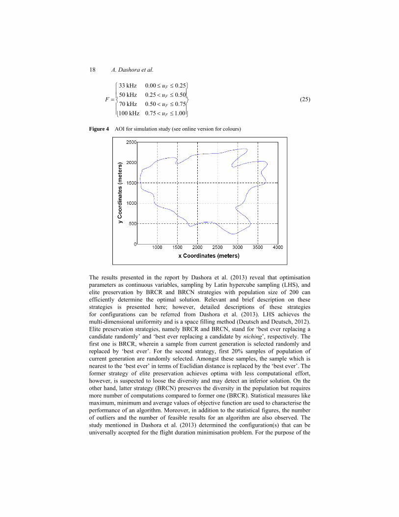
In view of the nature of objective function and characteristics of variables of design vector specific to the flight planning problem, a simulation study is first conducted on an arbitrary shaped AOI. The arbitrarily shaped simulated AOI, which occupies approximately 4 km2 area on map, is shown in local map coordinates in Figure 4. The difference between the maximum and minimum elevation point is assumed to be 200 metres.

A thorough investigation with the possible configurations of RGA code has been done for the flight planning problem for simulated AOI (Dashora et al., 2013). Optimisation parameters or variables of design vector in optimisation problem are considered continuous variables, i.e., integer variables (half scan angle, scanning frequency) are obtained by rounding the continuous variable to the nearest integer. However, as shown in Table 2, for ALTM 3100EA scanner, the discrete variable like PRF is a discontinuous variable and is a function of flying height (H) which is a continuous parameter. A continuous random variable (uF) is generated in the range [0 1] and mapped to discrete values of PRF as following:

( )( )( )( )

1.00 80 1,1000.75 1,100 1,7000.50 1,700 2,5000.25 2,500 3,500

F

FF

F

F

u Hu H

uu Hu H

⎧ ⎫≤ ≤⎪ ⎪< ≤⎪ ⎪= ⎨ ⎬

< ≤⎪ ⎪⎪ ⎪< ≤⎩ ⎭

(24)


33 kHz 0.00 0.2550 kHz 0.25 0.5070 kHz 0.50 0.75100 kHz 0.75 1.00

F

F

F

F

uu

Fuu

≤ ≤⎧ ⎫⎪ ⎪< ≤⎪ ⎪= ⎨ ⎬< ≤⎪ ⎪⎪ ⎪< ≤⎩ ⎭

(25)

Figure 4 AOI for simulation study (see online version for colours)

The results presented in the report by Dashora et al. (2013) reveal that optimisation parameters as continuous variables, sampling by Latin hypercube sampling (LHS), and elite preservation by BRCR and BRCN strategies with population size of 200 can efficiently determine the optimal solution. Relevant and brief description on these strategies is presented here; however, detailed descriptions of these strategies for configurations can be referred from Dashora et al. (2013). LHS achieves the multi-dimensional uniformity and is a space filling method (Deutsch and Deutsch, 2012). Elite preservation strategies, namely BRCR and BRCN, stand for ‘best ever replacing a candidate randomly’ and ‘best ever replacing a candidate by niching’, respectively. The first one is BRCR, wherein a sample from current generation is selected randomly and replaced by ‘best ever’. For the second strategy, first 20% samples of population of current generation are randomly selected. Amongst these samples, the sample which is nearest to the ‘best ever’ in terms of Euclidian distance is replaced by the ‘best ever’. The former strategy of elite preservation achieves optima with less computational effort, however, is suspected to loose the diversity and may detect an inferior solution. On the other hand, latter strategy (BRCN) preserves the diversity in the population but requires more number of computations compared to former one (BRCR). Statistical measures like maximum, minimum and average values of objective function are used to characterise the performance of an algorithm. Moreover, in addition to the statistical figures, the number of outliers and the number of feasible results for an algorithm are also observed. The study mentioned in Dashora et al. (2013) determined the configuration(s) that can be universally accepted for the flight duration minimisation problem. For the purpose of the


completeness of the suggested two-step procedure, the results of best configurations of algorithmic strategies, which are listed in Dashora et al. (2013), are directly adopted and presented in Table 4. Table 4 Statistical results of simulation of test problem with algorithms ABRCR to ABRCN

Algorithm Minimum(seconds)

Maximum(seconds)

Average(seconds)

Standard dev.(seconds)

Outliers/ feasible results

ABRCR (RCV + LHS + BRCR)

1,941.770 1,948.097 1,944.136 1.804 1/30

ABRCN (RCV + LHS + BRCN)

1,942.317 1,949.325 1,944.609 2.069 0/30

GA successfully resolved MINLP of flight problem which classical methods could not handle efficiently. Following are the critical observations:

a GA, being free of any assumption and without any estimate about the initial point, could reach very close to the global optima. The solution obtained by GA can be used as initial guess or initial point for the classical method.

b The scanner parameters, which are either integer variables or discrete variables, are detected by the GA with higher confidence as their values are constants over multiple runs of GA. However, the flying parameters (flying height, flying speed and flying direction), which are mathematically continuous variables, display variation from run to run.

c None of the algorithms is free of outliers. In addition to that, the standard deviation of the flight duration, which is the measure of consistency for an algorithm, also shows variation from run to run. Even increasing the population size cannot improve its consistency or reduce the standard deviation.

As a result of the above observation, the scanner parameters (half scan angle, scanning frequency, PRF) can be considered constant and classical method can be used to further optimise the flying parameters (flying height, flying speed, flying direction) for the convergence. Therefore, after rejecting the outliers, the solutions obtained by the algorithms ABRCR and ABRCN for two problems with the population size of 200, are supplied as the initial guesses for the HJ method. During the iterations in HJ method, a solution is accepted if it provides less value of flight duration and satisfies all constraints.

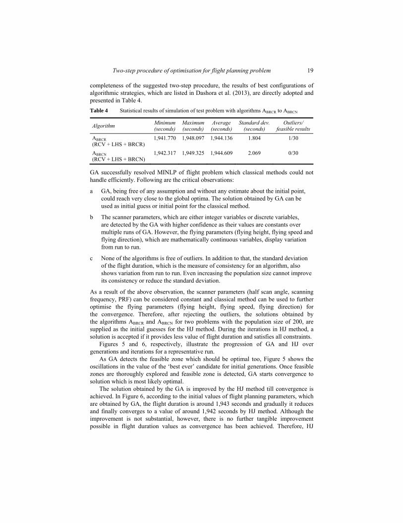
Figures 5 and 6, respectively, illustrate the progression of GA and HJ over generations and iterations for a representative run.

As GA detects the feasible zone which should be optimal too, Figure 5 shows the oscillations in the value of the ‘best ever’ candidate for initial generations. Once feasible zones are thoroughly explored and feasible zone is detected, GA starts convergence to solution which is most likely optimal.

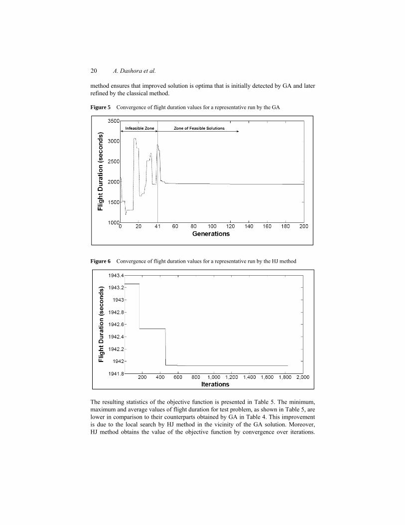
The solution obtained by the GA is improved by the HJ method till convergence is achieved. In Figure 6, according to the initial values of flight planning parameters, which are obtained by GA, the flight duration is around 1,943 seconds and gradually it reduces and finally converges to a value of around 1,942 seconds by HJ method. Although the improvement is not substantial, however, there is no further tangible improvement possible in flight duration values as convergence has been achieved. Therefore, HJ


method ensures that improved solution is optima that is initially detected by GA and later refined by the classical method.

Figure 5 Convergence of flight duration values for a representative run by the GA

Figure 6 Convergence of flight duration values for a representative run by the HJ method

The resulting statistics of the objective function is presented in Table 5. The minimum, maximum and average values of flight duration for test problem, as shown in Table 5, are lower in comparison to their counterparts obtained by GA in Table 4. This improvement is due to the local search by HJ method in the vicinity of the GA solution. Moreover, HJ method obtains the value of the objective function by convergence over iterations.


Figure 6 shows the convergence of HJ method for one of the initial guesses, obtained by GA. However, it is interesting to note that due to the improvement in the results of GA by HJ method, the standard deviation of the HJ results are sometimes higher than the initial guess provided by GA solutions. Table 5 Statistical results of simulation of test problems P2 and P4 with hybrid algorithm

Algorithm Minimum (seconds)

Maximum (seconds)

Average (seconds)

Standard dev. (seconds)

ABRCR (RCV + LHS + BRCR)

1,941.619 1,947.964 1,943.218 1.921

ABRCN (RCV + LHS + BRCN)

1,941.086 1,948.352 1,943.349 2.026

It may be noted that though there is an insignificant improvement by HJ method, the purpose of this discussion is to show the utility of GA supported by classical method for reaching the minima with convergence.

7 Implementation of two-step procedure for actual test site

7.1 Details of AOI site data requirements, and sensors

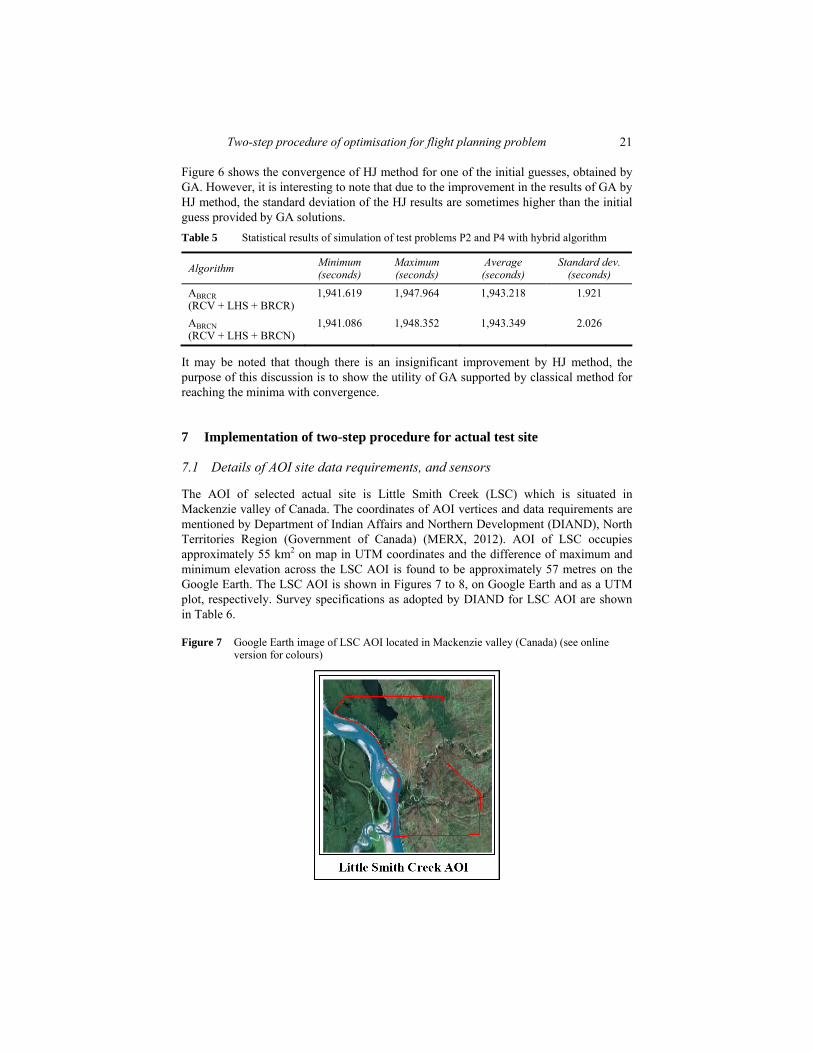
The AOI of selected actual site is Little Smith Creek (LSC) which is situated in Mackenzie valley of Canada. The coordinates of AOI vertices and data requirements are mentioned by Department of Indian Affairs and Northern Development (DIAND), North Territories Region (Government of Canada) (MERX, 2012). AOI of LSC occupies approximately 55 km2 on map in UTM coordinates and the difference of maximum and minimum elevation across the LSC AOI is found to be approximately 57 metres on the Google Earth. The LSC AOI is shown in Figures 7 to 8, on Google Earth and as a UTM plot, respectively. Survey specifications as adopted by DIAND for LSC AOI are shown in Table 6.

Figure 7 Google Earth image of LSC AOI located in Mackenzie valley (Canada) (see online version for colours)


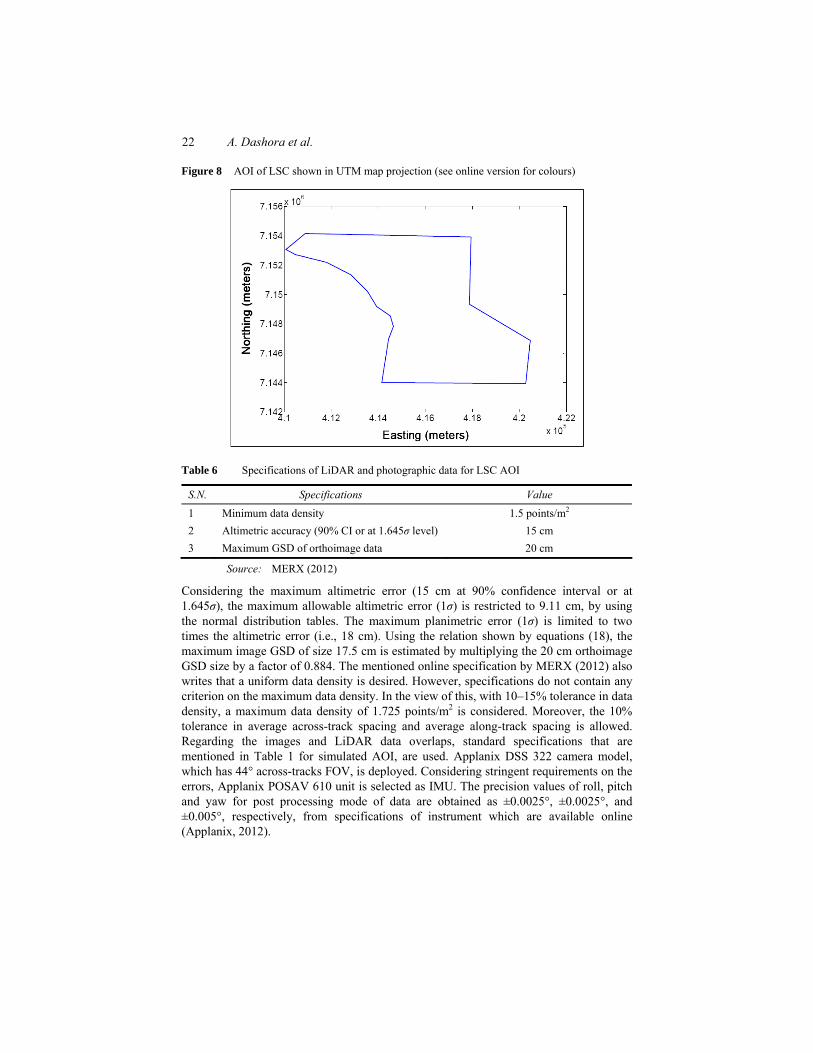
Figure 8 AOI of LSC shown in UTM map projection (see online version for colours)

Table 6 Specifications of LiDAR and photographic data for LSC AOI

S.N. Specifications Value

1 Minimum data density 1.5 points/m2 2 Altimetric accuracy (90% CI or at 1.645σ level) 15 cm 3 Maximum GSD of orthoimage data 20 cm

Source: MERX (2012)

Considering the maximum altimetric error (15 cm at 90% confidence interval or at 1.645σ), the maximum allowable altimetric error (1σ) is restricted to 9.11 cm, by using the normal distribution tables. The maximum planimetric error (1σ) is limited to two times the altimetric error (i.e., 18 cm). Using the relation shown by equations (18), the maximum image GSD of size 17.5 cm is estimated by multiplying the 20 cm orthoimage GSD size by a factor of 0.884. The mentioned online specification by MERX (2012) also writes that a uniform data density is desired. However, specifications do not contain any criterion on the maximum data density. In the view of this, with 10–15% tolerance in data density, a maximum data density of 1.725 points/m2 is considered. Moreover, the 10% tolerance in average across-track spacing and average along-track spacing is allowed. Regarding the images and LiDAR data overlaps, standard specifications that are mentioned in Table 1 for simulated AOI, are used. Applanix DSS 322 camera model, which has 44° across-tracks FOV, is deployed. Considering stringent requirements on the errors, Applanix POSAV 610 unit is selected as IMU. The precision values of roll, pitch and yaw for post processing mode of data are obtained as ±0.0025°, ±0.0025°, and ±0.005°, respectively, from specifications of instrument which are available online (Applanix, 2012).


7.2 Statistical performance of GA

Simulations are performed for 30 runs with ABRCR and ABRCN algorithms. Initially, flight planning is performed with 10% tolerance in data density. However, algorithms ABRCR and ABRCN failed to detect a feasible solution. Therefore, tolerance in data density is increased to 15%. Following results, as shown in Table 7, are obtained by GA. Table 7 Statistical results of simulation for LSC AOI with algorithms ABRCR and ABRCN


Maximum (seconds)

Average (seconds)


Outliers/ feasible results

ABRCR 3,304.78 3,457.65 3,366.58 41.23 2/30 ABRCN 3,196.92 3,255.57 3,230.59 20.16 0/30

Results in Table 7 show that both algorithms ABRCR and ABRCN can perform under the specified requirements. It is also observed that algorithm ABRCR detects two flying directions for LSC AOI. This is due to the fact that the flight durations in two directions are similar. Contrary to this, the algorithm ABRCN, though detects a single flying direction, shows higher value of standard deviation. Therefore, in view of the performance as listed above, both algorithms ABRCR and ABRCN should be attempted for flight planning problems and the better result should be used. According to the flying height obtained, LSC AOI is relatively flat as the relief ratio (PR) is less than 10%. The high variations in the scanning frequency and aircraft speed are due to the adopted value of tolerance in data density (15%) for a minimum data density of 1.5 points/m2 which is very small quantity. Moreover, the scan frequency (f) and the aircraft speed (V) show considerable variation while the half scan angle (φ) show less variation. The results obtained by GA are employed as the initial guess to the HJ method.

7.3 Simulation performance of refinement of GA results by HJ method

If GA results are improved by HJ method, results of latter method (HJ method) are accepted as refinement over the results provided by former (GA). The statistics of the results obtained by the two-step procedure, which is a hybrid method, are shown in Table 8. As shown in Table 8, minimum, maximum and the average of the flight duration values have improved over the results of GA. Due to this improvement, which occurs to some of the values, the standard deviation has become larger. Table 8 Statistical results of hybrid algorithm for LSC AOI


Maximum (seconds)

Average (seconds)


ABRCR 3,174.15 3,457.65 3,263.67 76.14 ABRCN 3,196.91 3,255.57 3,230.57 20.15


8 Flight plan of AOIs with optimal parameters obtained by two-step procedure

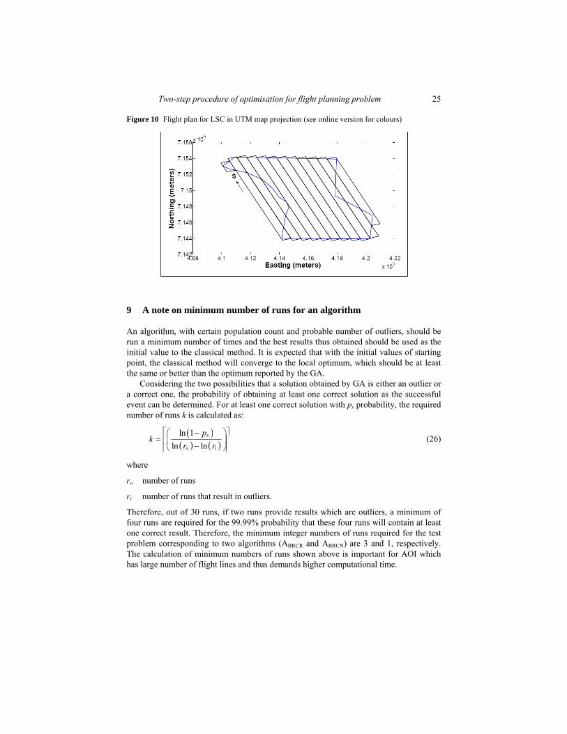
The obtained parameters of flight planning by the two-step procedure for the simulated AOI and LSC AOI are shown in Table 9. Out of all results of two-step procedure, the best results that provide the minimum flight durations for the simulated AOI as well as LSC AOI are selected and flight plans are drawn, as shown in Figures 9 to 10, respectively. Flight plans are showing the flight strips for the two AOIs. Point S in the figures show the starting point of aerial operation on map for data acquisition and the arrow indicates the flying direction on the first flight line which is originating from point S. Table 9 Flight planning parameters for AOIs by two-step procedure of optimisation

AOI name φ (deg)

f (Hz)

H (m)

V (m/s)

θ (deg)

F (kHz)

FD (seconds)

Simulated AOI 7 70 886.3 45.9 9.875 100 1,942. 6 LSC AOI 18 38 1,156.6 62.1 110.36 70 3,174.2

Figure 9 Flight plan for simulated AOI shown in local map projection (see online version for colours)

It is interesting to observe in Figure 10 shows that two-step procedure of optimisation detects the flight direction along the longest direction of LSC AOI. The longest direction is reported more economical by other authors also than any other direction, as it results in minimum number of turns (Read and Graham, 2002; Piel and Populus, 2007). However, also for an AOI as for simulated AOI in Figure 9, the two-step procedure of optimisation detects the most optimal direction for the given data requirements.


Figure 10 Flight plan for LSC in UTM map projection (see online version for colours)

9 A note on minimum number of runs for an algorithm

An algorithm, with certain population count and probable number of outliers, should be run a minimum number of times and the best results thus obtained should be used as the initial value to the classical method. It is expected that with the initial values of starting point, the classical method will converge to the local optimum, which should be at least the same or better than the optimum reported by the GA.

Considering the two possibilities that a solution obtained by GA is either an outlier or a correct one, the probability of obtaining at least one correct solution as the successful event can be determined. For at least one correct solution with ps probability, the required number of runs k is calculated as:

( )( ) ( )ln 1

ln lns

o t

pk

r r⎡ ⎤⎛ ⎞−

= ⎢ ⎥⎜ ⎟−⎝ ⎠⎢ ⎥ (26)

where

ro number of runs

rt number of runs that result in outliers.

Therefore, out of 30 runs, if two runs provide results which are outliers, a minimum of four runs are required for the 99.99% probability that these four runs will contain at least one correct result. Therefore, the minimum integer numbers of runs required for the test problem corresponding to two algorithms (ABRCR and ABRCN) are 3 and 1, respectively. The calculation of minimum numbers of runs shown above is important for AOI which has large number of flight lines and thus demands higher computational time.


10 Conclusions

This paper describes the flight planning problem for airborne LiDAR and simultaneous photographic data acquisition in the form of objective function and constraints. Flight duration, which is the objective function, is taken as the sum of the strip time and turning time. Due to turning from one flight line to another, flight duration is a discontinuous function. The variables involved in the objective function and constraints are studied and classified into the scanner parameters and the flying parameters. Scanner parameters are found to be integer and discrete parameters whereas the flying parameters are continuous parameters. Furthermore, it is noted that due to the absence of any estimate of solution, the classical methods of optimisation cannot be used. As a result, GA, which is an evolutionary algorithm, are proposed as an optimisation technique. On the other hand, due to the very large time required by GA for the convergence, a two-step procedure comprising of GA and HJ method of classical optimisation is attempted. For a study conducted with two-step procedure for the simulated AOI, it is observed that GA detects the optima with higher confidence in scanner parameters and varying flying parameters over multiple runs. The minimum, maximum, average and standard deviation of the objective function with the number of outliers are observed. The solutions obtained by GA by multiple runs with constant scanner parameters are provided as initial point to classical method for optimising the flying parameters. HJ method is found to further improve the optimal results. The improvement is indicated by the reduction in the maximum and minimum values of the objective function. The two-step procedure is implemented on an actual test site situated in Mackenzie valley of Canada with different data requirements. The suggested approach successfully obtained the results by GA followed by HJ method. Finally, for larger areas, which may need a large number of flight lines, a procedure is given to calculate the minimum number of runs for acceptable results. The results obtained in this study prove that the suggested approach of flight planning using GA is successful and can be applied for the similar problems. This is a novel attempt to use GA for flight planning and has potential for commercial applications.

References Applanix (2012) POSAV Specifications [online] http://www.applanix.com/media/downloads/

products/specs/POSAV_SPECS_OLD.pdf (accessed 28 May 2013). Baltsavias, E.P. (1999) ‘Airborne laser scanning: basic relations and formulas’, ISPRS Journal of

Photogrammetry & Remote Sensing, Vol. 54, pp.199–214. Bang, K.I., Kersting, A.P., Habib, A. and Lee, D.C. (2009) ‘LiDAR system calibration using point

cloud coordinates in overlapping strips’, ASPRS 2009 Annual Conference, 9–13 March 2009, Baltimore, Maryland, 12p.

Benavent, E., Corberan, A., Pinana, E., Plana, I. and Sanchis, J.M. (2005) ‘New heuristic algorithms for the windy rural postman problem’, Computers and Operation Research, Vol. 32, pp.3111–3128.

Costa, L., Santo, I.A.C.P.E. and Fernandes, E.M.G.P. (2012) ‘A hybrid genetic pattern search augmented method for constrained global optimization’, Applied Mathematics and Computations, Vol. 218, pp.9415–9426.

Dashora, A. (2013) Optimization System for Flight Planning for Airborne LiDAR Data Acquisition, PhD dissertation, Indian Institute of Technology Kanpur, Kanpur, India.


Dashora, A. and Lohani, B. (2013a) Turning Time Calculation for Airborne Surveys, KanGAL Report No. 2013010, Indian Institute of Technology Kanpur, Kanpur, India [online] http://www.iitk.ac.in/kangal/reports.shtml (accessed 26 May 2013).

Dashora, A. and Lohani, B. (2013b) Calculation of Error Propagated in Airborne LiDAR Data, KanGAL Report No. 2013011, Indian Institute of Technology Kanpur, Kanpur, India [online] http://www.iitk.ac.in/kangal/reports.shtml (accessed 26 May 2013).

Dashora, A., Lohani, B. and Deb, K. (2013) Solving Flight Planning Problem for Airborne LiDAR Data Acquisition using Single and Multi-objective Genetic Algorithms, KanGAL Report No. 2013012, Indian Institute of Technology Kanpur, Kanpur, India [online] http://www.iitk.ac. in/kangal/reports.shtml (accessed 28 May 2013).

Deutsch, J.L. and Deutsch, C.V. (2012) ‘Latin hypercube sampling with multidimensional uniformity’, Journal of Statistical Planning and Inference, Vol. 142, pp.763–772.

DGCA (2010) ‘Establishments of minimum flight altitudes’, Section 9 – Air Space and Air Traffic Management, Civil Aviation Requirements, Series ‘R’, – Air Routes, Part I, No. 2, Office of Director General of Civil Aviation, New Delhi, India [online] http://dgca.nic.in/cars/D9R-R1.pdf (accessed 1 May 2012).

DWMI (2007) Digital World Mapping Inc.: LiDAR US LLC [online] http://www.lidarus.com/ oil.html (accessed 14 January 2009).

Fernandes, F.P., Costa, M.P.F. and Fernandes, E.M.G.P. (2011) ‘Assessment of a hybrid approach for nonconvex constrained MINLP problems’, Proceedings of the 11th International Conference on Computational and Mathematical Methods in Science and Engineering, CMMSE 2011, 26–30 June 2011, Benidorm, Alicante, Spain, 14 pages.

Glennie, C. (2007) ‘Rigorous 3D error analysis of kinematic scanning LiDAR systems’, Journal of Applied Geodesy 1, Journal of Applied Geodesy 1, Vol. 1, No. 3, pp.147-157.

Goldberg, D.E. (1989) ‘A gentle introduction to genetic algorithms’, Genetic Algorithms in Search, Optimization, and Machine Learning, pp.1–25, Pearson Education Asia, Delhi, India.

Grendzdörffer, G.J. (2008) ‘Medium format digital cameras – A EuroSDR project’, The International Archives of Photogrametry, Remote Sensing and Spatial Information Science, XXXVII, Part B1, Beijing, pp.1043-1049.

Hofton, M.A., Blair, J.B., Minster, B., Ridgway, J.R., Williams, N.P., Bufton, J.L. and Rabine, D.L. (2000) ‘An airborne scanning laser altimetry survey of long valley, California’, International Journal of Remote Sensing, Vol. 21, pp.2413–2437.

Jake Carroll, Private Communication, E-mail Communication on 20 February 2009 with Mr. Jack Carroll, Bearing Tree Land Surveying L.L.C., Oklahoma City, USA.

Jenkins, J. (2013) ‘Key drivers in determining LiDAR sensor selection’, Promoting Land Adminsitration and Good Governance, 5th FIG Regional Conference, 8–11 March 2006, Accra, Ghana, 18p.

Kaupe Jr., A.F. (1963) ‘Algorithm 178: direct search’, Communications of ACM, Vol. 6, No. 6, pp.313–314.

Landtwing, S. and Whitcare, J. (2008) ‘Simultaneous data acquisition with airborne LiDAR and largeformat digital camera’, International LiDAR Mapping Forum 2008 Denver, 11p [online] http://www.swissphoto.ch/fileadmin/content/documents/1_3D-Mapping/2008-02_ SensorFusion_Landtwing_Whitacre_ILMF.pdf (accessed 27 June 2012).

Mariusz Boba, Private Communication, E-mail Communication on 19 February 2009 with Mariusz Boba, Optech Inc., Canada.

MERX (2012) Advance Contract Award Notice – LiDAR Acquisition at 8 Stream Crossing Sites in the Mackenzie Valley, Yellowknife, Northwest Territories, Canada [online] http://www.merx.com/English/SUPPLIER_Menu.asp?WCE=Show&TAB=1&PORTAL=MERX&State=7&id=213336&src=osr&FED_ONLY=0&ACTION=&rowcount=&lastpage=&MoreResults=&PUBSORT=0&CLOSESORT=0&hcode=rl3FGHg0ccv11LdRDqrBow%3D%3D (accessed 10 December 2012).


Optech (2006a) ALTM 3100EA Specifications, Optech Inc., Canada [online] http://www.optech.ca (accessed 15 January 2009).

Optech (2006b) Digital Camera APPLANIX, Optech Inc., Canada [online] http://www.optech.ca/ pdf/ALTMApplanixPC.pdf (accessed 12 September 2012).

Piel, S. and Populus, J. (2007) Recommended Operating Guidelines (ROG) for LiDAR Surveys, 19p, MESH Guidance Publication, Ver-3, Mapping European Seabed Habitats (MESH) [online] http://www.searchmesh.net/PDF/GMHM3_LIDAR_ROG.pdf (accessed 15 July 2012).

Read, R. and Graham, R. (2002) Manual of Aerial Survey: Primary Data Acquisition, 408p, Whittles Publishing, Scottland, UK.

RICS (2010) Vertical Aerial Photography and Digital Imagery, 5th ed., 59p, RICS Guidance Note (GN 61/2010), Royal Institution of Chartered Surveyors, Coventry, UK.

Rodrigues, A.M. and Ferreira, S. (2012) ‘Cutting path as a rural postman problem: solutions by memetic algorithms’, International Journal of Combinatorial Optimization Problems and Informatics, Vol. 3, No. 1, pp.31–46.

Saylam, K. (2009) ‘Quality assurance of LiDAR system-mission planning’, ASPRS 2009 Annual Conference, 9–13 March 2009, Baltimore, Maryland, 13p.

Shih, P.T.Y. and Huang, C.M. (2009) ‘The building shadow problem of airborne LiDAR’, The Photogrammetric Record, Vol. 24, No. 128, pp.372–385.

USGS (2010) ‘USGS NGP LiDAR guidelines and base specifications’, United States Geological Survey, National Geospatial Program, International LiDAR Mapping Forum 2010, Version-13, 18p.

Wehr, A. and Lohr, U. (1999) ‘Airborne laser scanning – an introduction and overview’, ISPRS Journal of Photogrammetry & Remote Sensing, Vol. 54, pp.68–82.

Documents

Ajay Dashora* Bharat Lohani Kalyanmoy Deb Procedure_IJMMNO_2013.pdf · scanning angle, scanning frequency and point repetition frequency) impose the ... method and also describe two-step