Embed Size (px)
Citation preview

RMMM 8 - 2017: Matheon Workshop - Reliable Methods of Mathematical Modeling Humboldt Universitat zu Berlin, Germany, August 2 2017
Functional A Posteriori Error Estimates (FAPEE)for Electro-Magneto Statics (EMS)
. . . and more
Dirk PaulyFakultat fur Mathematik
RMMM 8 - Berlin 2017Matheon Workshop - Reliable Methods of Mathematical Modeling
August 2 2017Humboldt Universitat zu Berlin, Germany
Dirk Pauly FAPEE for EMS . . . and more Universitat Duisburg-Essen, Campus Essen

RMMM 8 - 2017: Matheon Workshop - Reliable Methods of Mathematical Modeling Humboldt Universitat zu Berlin, Germany, August 2 2017
First Order Model Problem
Model Problem: Electro-Magneto-Static Maxwell Equations
setting: Hilbert/L2-based Sobolev spacesgeometry: Ω ⊂ R3 bounded domain with weak Lipschitz boundary Γ = ∂Ω
rotE = J in Ω (1)
−div εE = j in Ω (2)
ν × E = 0 at Γt (3)
ν ⋅ εE = 0 at Γn (4)
non-trivial kernel: HD,ε = H ∈ L2 ∶ rotH = 0, div εH = 0, ν ×H ∣Γt = 0, ν ⋅ εH ∣Γn = 0additional condition on Dirichlet/Neumann fields for uniqueness:
πDE = H ∈HD,ε (5)
well known: (1)-(5) uniquely solvable by Helmholtz decompositions andFriedrichs/Poincare/Maxwell type estimates for given right hand sides F , G , H
aim: functional a posteriori error estimates (FAPEE) for electro-magneto statics(EMS) – simple and easy estimates
Dirk Pauly FAPEE for EMS . . . and more Universitat Duisburg-Essen, Campus Essen

RMMM 8 - 2017: Matheon Workshop - Reliable Methods of Mathematical Modeling Humboldt Universitat zu Berlin, Germany, August 2 2017
First Order Model Problem
Model Problem: Electro-Magneto-Static Maxwell Equations
literature: not very much
for rot rot + 1 (second order toy equation):
residual based: Beck/Hoppe/Hiptmair/Wohlmuth (’00)Creuse/Nicaise/. . . (’03)Schoberl (’08)
functional: Anjam/Neittaanmaki/Repin (’07)Anjam/P. (’16, ’17)
for rot rot (second order equation):
residual based: Creuse/Nicaise/. . . (’14, ’15)equilibrated: Braess/Schoberl (’08)
functional: P./Repin (’09)
for first order rot/div-system of EMS: nothing (to the best of our knowledge)
Dirk Pauly FAPEE for EMS . . . and more Universitat Duisburg-Essen, Campus Essen

RMMM 8 - 2017: Matheon Workshop - Reliable Methods of Mathematical Modeling Humboldt Universitat zu Berlin, Germany, August 2 2017
First Order Model Problem
Model Problem: Main Result for Electro-Magneto-Static Maxwell Equations
Theorem (sharp upper bounds)
Let E ∈ L2ε (very non-conforming!) and e ∶= E − E . Then
∣e∣2L2ε= ∣π∇e∣
2L2ε+ ∣πrote∣
2L2ε+ ∣πDe∣
2L2ε
= minΦ∈HΓn (div ε)
(cfp∣div εΦ + j ∣L2 + ∣Φ − E ∣L2ε)
2reg. (−∇Γt
divΓn +1)-prbl. in HΓn (div)
+ minΦ∈HΓt
(rot)(cm∣ rot Φ − J ∣L2 + ∣Φ − E ∣L2
ε)
2reg. (rotΓn rotΓt
+1)-prbl. in HΓt(rot)
+ minφ∈H1
Γt,Ψ∈HΓn (rot)
∣∇φ + ε−1 rot Ψ + E −H ∣2L2ε.
cpld. (− divΓn ∇Γt)-(rotΓt
rotΓn )-sys. in H1Γt
-HΓn (rot)
Remark
(rotΓt rotΓn)-prbl. (Dirichlet/Neumann fields err.) needs saddle point form..
Ω top. trv. ⇒ πD = 0 and HΓt (rot 0) = ∇H1Γt
and HΓn(div 0) = rot HΓn(rot)
Ω convex (and ε = µ = 1) and Γt = Γ or Γn = Γ⇒ cf ≤ cm ≤ cp ≤ diamΩ /π
⇒ all constants known
Dirk Pauly FAPEE for EMS . . . and more Universitat Duisburg-Essen, Campus Essen

RMMM 8 - 2017: Matheon Workshop - Reliable Methods of Mathematical Modeling Humboldt Universitat zu Berlin, Germany, August 2 2017
First Order Model Problem
Underlying Structure of the Model Problem
∇-rot-div-complex (de Rham complex):
0 or Rιπ
L2∇Γt
− divΓn εL2ε
rotΓt
ε−1 rotΓn
L2divΓt
−∇Γn
L2 πι
R or 0
unbounded, densely defined, closed, linear operators with adjoints
∇Γt ∶ H1Γt⊂ L2
→ L2ε, −divΓn ε = (∇Γt )
∗∶ ε−1DΓn ⊂ L2
ε → L2 sometimes:
rotΓt ∶ RΓt ⊂ L2ε → L2, ε−1 rotΓn = (rotΓt )
∗∶ RΓn ⊂ L2
→ L2ε R = H(rot) = H(curl)
divΓt ∶ DΓt ⊂ L2→ L2, −∇Γn = (divΓt )
∗∶ H1
Γn⊂ L2
→ L2 D = H(div)
complex: ‘range ⊂ kernel’ (rot∇ = 0, div rot = 0)
∇Γt H1Γt⊂ RΓt ,0, rotΓt RΓt ⊂ DΓt ,0, divΓt DΓt ⊂ N(π) = L2 or L2
crucial: compact embeddings (Rellich’s selection theorem & Weck’s selection theorem)
H1 L2, RΓt ∩ ε
−1DΓn L2
⇒ Helmholtz decompositions, closed ranges, continuous inverses, andFriedrichs/Poincare/Maxwell type estimates
√
Weck’s selection theorem (Weck ’74, (Habil.) stimulated by Rolf Leis)(Weber ’80, Picard ’84, Costabel ’90, Witsch ’93, Jochmann ’97, Kuhn ’99,Picard/Weck/Witsch ’01, Bauer/P./Schomburg ’16, ’17)
Dirk Pauly FAPEE for EMS . . . and more Universitat Duisburg-Essen, Campus Essen

RMMM 8 - 2017: Matheon Workshop - Reliable Methods of Mathematical Modeling Humboldt Universitat zu Berlin, Germany, August 2 2017
First Order Model Problem
Abstract Formulation
rotE = J in Ω
−div εE = j in Ω
ν × E = 0 at Γt
ν ⋅ εE = 0 at Γn
πDE = H ∈HD,ε
£
rotΓt E = J
−divΓn εE = j
πDE = H ∈HD,ε
(Ai ∶= rotΓt , A∗i = ε
−1 rotΓn) £ (x ∶= E) (Ai−1 ∶= ∇Γt , A∗i−1 = −divΓn ε)
Aix = f
A∗i−1x = g
πix = h ∈Hi ∶= N(Ai) ∩N(A∗i−1)
Dirk Pauly FAPEE for EMS . . . and more Universitat Duisburg-Essen, Campus Essen

RMMM 8 - 2017: Matheon Workshop - Reliable Methods of Mathematical Modeling Humboldt Universitat zu Berlin, Germany, August 2 2017
General First Order Problem
General or Abstract Problem
setting: unbounded, densely defined, closed, linear operators with adjoints
Ai ∶ D(Ai) ⊂ Hi → Hi+1, A∗i ∶ D(A
∗i ) ⊂ Hi+1 → Hi , i ∈ Z
complex:
. . . Hi−2
Ai−2
A∗i−2
Hi−1
Ai−1
A∗i−1
Hi
AiA∗
i
Hi+1
Ai+1
A∗i+1
Hi+2 . . .
complex property: ‘range ⊂ kernel’ ( AiAi−1 = 0 ⇔ A∗i−1A
∗i = 0)
R(Ai−1) ⊂ N(Ai) ⇔ R(A∗i ) ⊂ N(A∗
i−1)
problem: find x ∈ D(Ai) ∩D(A∗i−1) s.t.
Aix = f , A∗i−1x = g , πix = h,
where f ∈ R(Ai), g ∈ R(A∗i−1) and h ∈Hi with kernel Hi ∶= N(Ai) ∩N(A∗
i−1)
Dirk Pauly FAPEE for EMS . . . and more Universitat Duisburg-Essen, Campus Essen

RMMM 8 - 2017: Matheon Workshop - Reliable Methods of Mathematical Modeling Humboldt Universitat zu Berlin, Germany, August 2 2017
General First Order Problem
Toolbox
Hodge/Helmholtz/Weyl decompositions:
Hi = N(Ai)⊕HiR(A∗
i ), Hi+1 = N(A∗i )⊕Hi+1
R(Ai)
⇒ reduce Ai , A∗i to N(Ai)
, N(A∗i )
⇒ injective reduced operators Ai , A∗i
⇒ A−1i , (A∗i )
−1 exist
⇒ complex for Ai , A∗i
crucial: compact embeddings
D(Ai) Hi (⇔ D(A∗i ) Hi+1)
⇒
⎧⎪⎪⎪⎪⎪⎪⎪⎪⎪⎪⎪⎪⎪⎨⎪⎪⎪⎪⎪⎪⎪⎪⎪⎪⎪⎪⎪⎩
(general) Friedrichs/Poincare/Maxwell type estimates
∀ϕ ∈ D(Ai) ∣ϕ∣Hi≤ ci ∣Aiϕ∣Hi+1
∀ψ ∈ D(A∗i ) ∣ψ∣Hi+1≤ ci ∣A
∗i ψ∣Hi
closed ranges R(Ai) = R(Ai), R(A∗i ) = R(A∗i )
continuous and compact invers operators A−1i , (A∗i )
−1
lots of Helmholtz type decompositions
best world: D(Ai) ∩D(A∗i−1) Hi ⇒ D(Ai) Hi
Dirk Pauly FAPEE for EMS . . . and more Universitat Duisburg-Essen, Campus Essen

RMMM 8 - 2017: Matheon Workshop - Reliable Methods of Mathematical Modeling Humboldt Universitat zu Berlin, Germany, August 2 2017
General First Order Problem
Abstract Problem and Goal
problem: find x ∈ D(Ai) ∩D(A∗i−1) s.t.
Aix = f
A∗i−1x = g
πix = h
Theorem (solution theory)
unique solution (cont. dpd. on data) ⇔ f ∈ R(Ai), g ∈ R(A∗i−1) and h ∈Hi
Proof.
x = A−1i f + (A∗i−1)
−1g + h
goal: functional a posteriori error estimates (fapee) ‘in the spirit of Repin’
For x ∈ Hi (very non-conforming!) estimate ∣x − x ∣Hiin terms of x , and f , g , h, and ci .
Dirk Pauly FAPEE for EMS . . . and more Universitat Duisburg-Essen, Campus Essen

RMMM 8 - 2017: Matheon Workshop - Reliable Methods of Mathematical Modeling Humboldt Universitat zu Berlin, Germany, August 2 2017
Functional A Posteriori Error Estimates for First Order Problem
Upper Bounds
problem: find x ∈ D(Ai) ∩D(A∗i−1) s.t. Aix = f , A∗
i−1x = g , πix = h
‘very’ non-conforming ‘approximation’ of x : x ∈ Hi
def., dcmp. err. e ∶= x − x = πAi−1e + πie + πA∗
ie ∈ Hi = R(Ai−1)⊕Hi
Hi ⊕HiR(A∗
i )
Theorem (sharp upper bounds I)
Let x ∈ Hi and e ∶= x − x . Then∣e∣2Hi
= ∣πAi−1e∣2Hi
+ ∣πie∣2Hi+ ∣πA∗
ie∣2Hi
,
∣πAi−1e∣Hi
= minφ∈D(A∗
i−1)(ci−1∣A
∗i−1φ − g ∣Hi−1
+ ∣φ − x ∣Hi), reg. (Ai−1A
∗i−1 + 1)-prbl. in D(A∗i−1)
∣πA∗ie∣Hi
= minϕ∈D(Ai )
(ci ∣Aiϕ − f ∣Hi+1+ ∣ϕ − x ∣Hi
), reg. (A∗i Ai + 1)-prbl. in D(Ai )
∣πie∣Hi= ∣πi x − h∣Hi
= minξ∈D(Ai−1),
ζ∈D(A∗i )
∣Ai−1ξ +A∗i ζ + x − h∣Hi
.
cpld. (A∗i−1Ai−1)-(AiA∗i )-sys. in D(Ai−1)-D(A
∗i )
Remark
Even πie = h − πi x and the minima are attained atφ = πAi−1
e + x , ϕ = πA∗ie + x , Ai−1ξ +A∗
i ζ = (πi − 1)x .
Dirk Pauly FAPEE for EMS . . . and more Universitat Duisburg-Essen, Campus Essen

RMMM 8 - 2017: Matheon Workshop - Reliable Methods of Mathematical Modeling Humboldt Universitat zu Berlin, Germany, August 2 2017
Functional A Posteriori Error Estimates for First Order Problem
Upper Bounds (with less computations)
problem: find x ∈ D(Ai) ∩D(A∗i−1) s.t. Aix = f , A∗
i−1x = g , πix = h
‘very’ conforming ‘approximation’ of x : x ∈ D(Ai) ∩D(A∗i−1)
setting φ = ϕ = x in latter theorem (or directly by Poincare type estimates) ⇒
∣e∣2D(Ai )∩D(A∗i−1)= ∣πAi−1
e∣2Hi+ ∣πie∣
2Hi+ ∣πA∗
ie∣2Hi
+ ∣Aie∣2Hi+1
+ ∣A∗i−1e∣
2Hi−1
≤ ∣πi x − h∣2Hi+ (1 + c2
i )∣Ai x − f ∣2Hi+1+ (1 + c2
i−1)∣A∗i−1x − g ∣2Hi−1
let
F(x) ∶= ∣πi x − h∣2Hi+ ∣Ai x − f ∣2Hi+1
+ ∣A∗i−1x − g ∣2Hi−1
least squares functional of the problem. set cm,i ∶= maxci , ci−1
Corollary (error equivalence with least squares functional)
Let x ∈ D(Ai) ∩D(A∗i−1) and e ∶= x − x . Then
1
1 + c2m,i
∣e∣2D(Ai )∩D(A∗i−1)≤ F(x) ≤ ∣e∣2D(Ai )∩D(A
∗i−1).
note ∣e∣2D(Ai )∩D(A
∗i−1)= F(x) + ∣πAi−1
e∣2Hi+ ∣πA∗
ie∣2Hi
note: also partial results for (part. conf. approx.) x ∈ D(Ai) or x ∈ D(A∗i−1)
Dirk Pauly FAPEE for EMS . . . and more Universitat Duisburg-Essen, Campus Essen

RMMM 8 - 2017: Matheon Workshop - Reliable Methods of Mathematical Modeling Humboldt Universitat zu Berlin, Germany, August 2 2017
Functional A Posteriori Error Estimates for First Order Problem
Upper Bounds (without harmonic fields)
problem: find x ∈ D(Ai) ∩D(A∗i−1) s.t. Aix = f , A∗
i−1x = g , πix = h
‘very’ non-conforming ‘approximation’ of x : x ∈ Hi 1 with x = Ai−1y +A∗i z + h
reasonable assumption (by num. method): e = x − x ∈ R(Ai−1)⊕HiR(A∗
i )HiHi
⇒ e = πAi−1e + πA∗
ie ∈ R(Ai−1)⊕Hi
R(A∗i )
⇒ no error in the ‘harmonic fields’ part ∣πie∣Hi
Theorem (sharp upper bounds II)
Let x ∈ Hi and e ∶= x − x HiHi . Then
∣e∣2Hi= ∣πAi−1
e∣2Hi+ ∣πA∗
ie∣2Hi
,
∣πAi−1e∣Hi
= minφ∈D(A∗
i−1)(ci−1∣A
∗i−1φ − g ∣Hi−1
+ ∣φ − x ∣Hi),
∣πA∗ie∣Hi
= minϕ∈D(Ai )
(ci ∣Aiϕ − f ∣Hi+1+ ∣ϕ − x ∣Hi
).
no (computation of) projector πi onto Hi needed!
Dirk Pauly FAPEE for EMS . . . and more Universitat Duisburg-Essen, Campus Essen

RMMM 8 - 2017: Matheon Workshop - Reliable Methods of Mathematical Modeling Humboldt Universitat zu Berlin, Germany, August 2 2017
Functional A Posteriori Error Estimates for First Order Problem
Lower Bounds
recall problem: find x ∈ D(Ai) ∩D(A∗i−1) s.t. Aix = f , A∗
i−1x = g , πix = h
‘very’ non-conforming ‘approximation’ of x : x ∈ Hi
error e = x − x = πAi−1e + πie + πA∗
ie ∈ Hi = R(Ai−1)⊕Hi
Hi ⊕HiR(A∗
i )
Theorem (sharp lower bounds)
Let x ∈ Hi and e ∶= x − x . Then
∣e∣2Hi= ∣πAi−1
e∣2Hi+ ∣πie∣
2Hi+ ∣πA∗
ie∣2Hi
≥ ∣πAi−1e∣2Hi
+ ∣πA∗ie∣2Hi
,
∣πAi−1e∣2Hi
= maxφ∈D(Ai−1)
(2⟨g , φ⟩Hi−1− ⟨2x +Ai−1φ,Ai−1φ⟩Hi
),
∣πA∗ie∣2Hi
= maxϕ∈D(A∗
i)(2⟨f , ϕ⟩Hi+1
− ⟨2x +A∗i ϕ,A
∗i ϕ⟩Hi
),
πie = h − πi x .
Remark
The maxima are attained at φ ∈ D(Ai−1) with Ai−1φ = πAi−1e and ϕ ∈ D(A∗
i ) withA∗
i ϕ = πA∗ie.
Dirk Pauly FAPEE for EMS . . . and more Universitat Duisburg-Essen, Campus Essen

RMMM 8 - 2017: Matheon Workshop - Reliable Methods of Mathematical Modeling Humboldt Universitat zu Berlin, Germany, August 2 2017
General Second Order Problem
Abstract Problem and Goal
problem: find x ∈ D(A∗i Ai) ∩D(A∗
i−1) s.t.
A∗i Aix = f
A∗i−1x = g
πix = h
equivalent mixed formulation (y ∶= Aix):find pair (x , y) ∈ (D(Ai) ∩D(A∗
i−1)) × (D(A∗i ) ∩ R(Ai)
´¹¹¹¹¹¹¹¹¹¹¹¹¹¹¹¹¹¹¹¹¹¹¹¹¹¹¹¹¹¹¹¹¹¹¹¹¹¹¹¹¹¸¹¹¹¹¹¹¹¹¹¹¹¹¹¹¹¹¹¹¹¹¹¹¹¹¹¹¹¹¹¹¹¹¹¹¹¹¹¹¹¹¹¹¶=D(A∗
i)
) s.t.
Aix = y , Ai+1y = 0
A∗i−1x = g , A∗
i y = f
πix = h, πi+1y = 0
cont. solution theory√
: x = A−1i y + (A∗i−1)
−1g + h and y = (A∗i )−1f
goal: functional a posteriori error estimates ‘in the spirit of Repin’
for (x , y) ∈ Hi ×Hi+1 (very non-conforming!)
estimate ∣(x , y) − (x , y)∣Hi×Hi+1in terms of x , and y , f , g , h, and ci
Dirk Pauly FAPEE for EMS . . . and more Universitat Duisburg-Essen, Campus Essen

RMMM 8 - 2017: Matheon Workshop - Reliable Methods of Mathematical Modeling Humboldt Universitat zu Berlin, Germany, August 2 2017
Functional A Posteriori Error Estimates for Second Order Problem
Upper Bounds
Theorem (sharp upper bounds)
Let (x , y) ∈ Hi ×Hi+1 and e ∶= (x , y) − (x , y) ∈ Hi ×Hi+1.Then πiex = h − πi x and (1 − πAi
)ey = −(1 − πAi)y and
∣ex ∣2Hi
= ∣πAi−1ex ∣
2Hi+ ∣πiex ∣
2Hi+ ∣πA∗
iex ∣
2Hi,
∣ey ∣2Hi+1
= ∣πAiey ∣
2Hi+1
+ ∣(1 − πAi)ey ∣
2Hi+1
as well as
∣πAiey ∣Hi+1
= minθ∈D(A∗
i)(ci ∣A
∗i θ − f ∣Hi
+ ∣θ − y ∣Hi+1), reg. (AiA
∗i + 1)-prbl. in D(A∗i )
∣(1 − πAi)ey ∣Hi+1
= ∣(1 − πAi)y ∣Hi+1
= minξ∈D(Ai )
∣Aiξ − y ∣Hi+1, (A∗i Ai )-prbl. in D(Ai )
∣πAi−1ex ∣Hi
= minφ∈D(A∗
i−1)(ci−1∣A
∗i−1φ − g ∣Hi−1
+ ∣φ − x ∣Hi), reg. (Ai−1A
∗i−1 + 1)-prbl. in D(A∗i−1)
∣πA∗iex ∣Hi
= minϕ∈D(Ai ),
ψ∈D(A∗i )
(∣ϕ − x ∣Hi+ ci ∣Aiϕ − ψ∣Hi+1
+ c2i ∣A
∗i ψ − f ∣Hi
).
cpld. (A∗i Ai + 1)-(AiA∗i + 1)-sys. in D(Ai )-D(A
∗i )
Dirk Pauly FAPEE for EMS . . . and more Universitat Duisburg-Essen, Campus Essen

RMMM 8 - 2017: Matheon Workshop - Reliable Methods of Mathematical Modeling Humboldt Universitat zu Berlin, Germany, August 2 2017
Functional A Posteriori Error Estimates for Second Order Problem
Lower Bounds
. . .
Dirk Pauly FAPEE for EMS . . . and more Universitat Duisburg-Essen, Campus Essen

RMMM 8 - 2017: Matheon Workshop - Reliable Methods of Mathematical Modeling Humboldt Universitat zu Berlin, Germany, August 2 2017
Applications to First Order Systems
Electro-Magneto-Static Maxwell
Ω ⊂ R3 bounded domain with weak Lipschitz boundary Γ = ∂Ω
rotΓt E = J ∈ rot RΓt in Ω
−divΓn εE = j ∈ div DΓn = L2 or L2 in Ω
ν × E = 0 at Γt
ν ⋅ εE = 0 at Γn
πDE = H ∈HD,ε = RΓt ,0 ∩ ε−1DΓn,0
⇒ E ∈ RΓt ∩ ε−1DΓn
Ai−1 ∶= ∇Γt ∶ H1Γt⊂ L2
→ L2ε, Ai ∶= rotΓt ∶ RΓt ⊂ L2
ε → L2
A∗i−1 = −divΓn ε ∶ ε−1DΓn ⊂ L2
ε → L2, A∗i = ε
−1 rotΓn ∶ RΓn ⊂ L2→ L2
ε
Dirk Pauly FAPEE for EMS . . . and more Universitat Duisburg-Essen, Campus Essen

RMMM 8 - 2017: Matheon Workshop - Reliable Methods of Mathematical Modeling Humboldt Universitat zu Berlin, Germany, August 2 2017
Applications to First Order Systems
Electro-Magneto-Static Maxwell
compact embeddings:
D(Ai−1) Hi−1 ⇔ H1Γt L2 (Rellich’s selection theorem)
D(Ai) Hi ⇔ RΓt ∩ ε−1 rot RΓn ⊂ RΓt ∩ ε
−1DΓn L2ε (Weck’s selection theorem)
ci−1 = cfp (Friedrichs/Poincare constant) and ci = cm (Maxwell constant)
∀ϕ ∈ D(Ai−1) ∣ϕ∣Hi−1≤ ci−1∣Ai−1ϕ∣Hi
⇔ ∀ϕ ∈ H1Γt
∣ϕ∣L2 ≤ cfp∣∇ϕ∣L2ε
∀φ ∈ D(A∗i−1) ∣φ∣Hi≤ ci−1∣A
∗i−1φ∣Hi−1
⇔ ∀Φ ∈ ε−1DΓn ∩∇H1Γt
∣Φ∣L2ε≤ cfp∣div εΦ∣L2
∀ϕ ∈ D(Ai) ∣ϕ∣Hi≤ ci ∣Aiϕ∣Hi+1
⇔ ∀Φ ∈ RΓt ∩ ε−1 rot RΓn ∣Φ∣L2
ε≤ cm∣ rot Φ∣L2
∀ψ ∈ D(A∗i ) ∣ψ∣Hi+1≤ ci ∣A
∗i ψ∣Hi
⇔ ∀Ψ ∈ RΓn ∩ rot RΓt ∣Ψ∣L2 ≤ cm∣ rot Ψ∣L2ε
Helmholtz decomposition:
Hi = R(Ai−1)⊕HiHi ⊕Hi
R(A∗i ) ⇔ L2
ε = ∇H1Γt⊕L2
εHD,ε ⊕L2
εε−1 rot RΓn
orthonormal projectors:
πAi−1∶ Hi → R(Ai−1), πA∗
i∶ Hi → R(A∗
i ), πi ∶ Hi →Hi
⇔ π∇Γt∶ L2ε → ∇H1
Γt, πε−1 rotΓn
∶ L2ε → ε−1 rot RΓn , πD ∶ L2
ε →HD,ε
Dirk Pauly FAPEE for EMS . . . and more Universitat Duisburg-Essen, Campus Essen

RMMM 8 - 2017: Matheon Workshop - Reliable Methods of Mathematical Modeling Humboldt Universitat zu Berlin, Germany, August 2 2017
Applications to First Order Systems
Electro-Magneto-Static Maxwell: Upper Bounds
Theorem (sharp upper bounds I)
Let E ∈ L2ε (very non-conforming!) and e ∶= E − E . Then
∣e∣2L2ε= ∣π∇Γt
e∣2L2ε+ ∣πε−1 rotΓn
e∣2L2ε+ ∣πDe∣
2L2ε
= minΦ∈ε−1DΓn
(cfp∣div εΦ + j ∣L2 + ∣Φ − E ∣L2ε)
2reg. (−∇Γt
divΓn+1)-prbl. in DΓn
+ minΦ∈RΓt
(cm∣ rot Φ − J ∣L2 + ∣Φ − E ∣L2ε)
2reg. (rotΓn
rotΓt+1)-prbl. in RΓt
+ minφ∈H1
Γt,Ψ∈RΓn
∣∇φ + ε−1 rot Ψ + E −H ∣2L2ε.
cpld. (− divΓn∇Γt
)-(rotΓtrotΓn
)-sys. in H1Γt
-RΓn
Remark
(rotΓt rotΓn)-prbl. needs saddle point formulation.
Ω top. trv. ⇒ πD = 0 and RΓt ,0 = ∇H1Γt
and DΓn,0 = rot RΓn
Ω convex and ε = µ = 1 and Γt = Γ or Γn = Γ⇒ cf ≤ cm ≤ cp ≤diamΩ
π
Dirk Pauly FAPEE for EMS . . . and more Universitat Duisburg-Essen, Campus Essen

RMMM 8 - 2017: Matheon Workshop - Reliable Methods of Mathematical Modeling Humboldt Universitat zu Berlin, Germany, August 2 2017
Applications to First Order Systems
Electro-Magneto-Static Maxwell: Upper Bounds
reas. asspt. (by num. meth.): L2ε ∋ E = ∇u + ε−1 rot V +H, u ∈ H1
Γt, V ∈ RΓn
⇒ e = E − E = π∇Γte + πε−1 rotΓn
e ∈ ∇H1Γt⊕L2
εε−1 rot RΓn L2
εHD,ε
⇒ no error in the ‘Dirichlet/Neumann fields’ part ∣πDe∣L2ε
Theorem (sharp upper bounds II)
Let E ∈ L2ε (very non-conforming!) and e ∶= E − E . Then
∣e∣2L2ε= ∣π∇Γt
e∣2L2ε+ ∣πε−1 rotΓn
e∣2L2ε
= minΦ∈ε−1DΓn
(cfp∣div εΦ + j ∣L2 + ∣Φ − E ∣L2ε)
2reg. (−∇Γt
divΓn+1)-prbl. in DΓn
+ minΦ∈RΓt
(cm∣ rot Φ − J ∣L2 + ∣Φ − E ∣L2ε)
2reg. (rotΓn
rotΓt+1)-prbl. in RΓt
Remark
no computation of projector πD onto HD,ε needed!
Ω convex (and ε = µ = 1) and Γt = Γ or Γn = Γ⇒ cf ≤ cm ≤ cp ≤diamΩ
π⇒ everything is computable!
Dirk Pauly FAPEE for EMS . . . and more Universitat Duisburg-Essen, Campus Essen

RMMM 8 - 2017: Matheon Workshop - Reliable Methods of Mathematical Modeling Humboldt Universitat zu Berlin, Germany, August 2 2017
Applications to Second Order Systems
Dirichlet/Neumann Laplace
Ω ⊂ R3 bounded domain with weak Lipschitz boundary Γ = ∂Ω
−div ε∇u = f ∈ L2 in Ω
u = 0 at Γt
ν ⋅ ε∇u = 0 at Γn
⇔ ∇u = E ∈ ∇H1Γt
rotE = 0 ∈ rot RΓt in Ω
−div εE = f ∈ L2 or L2 in Ω
u = 0 ν × E = 0 at Γt
ν ⋅ εE = 0 at Γn
πDE = 0 ∈HD,ε
⇒ (u,E) ∈ H1Γt× (ε−1DΓn ∩∇H1
Γt)
Ai ∶= ∇Γt ∶ H1Γt⊂ L2
→ L2ε, Ai+1 ∶= rotΓt ∶ RΓt ⊂ L2
ε → L2
A∗i = −divΓn ε ∶ ε−1DΓn ⊂ L2
ε → L2, A∗i+1 = ε
−1 rotΓn ∶ RΓn ⊂ L2→ L2
ε
Dirk Pauly FAPEE for EMS . . . and more Universitat Duisburg-Essen, Campus Essen
RMMM 8 - 2017: Matheon Workshop - Reliable Methods of Mathematical Modeling Humboldt Universitat zu Berlin, Germany, August 2 2017
Applications to Second Order Systems
Dirichlet/Neumann Laplace: Upper Bounds
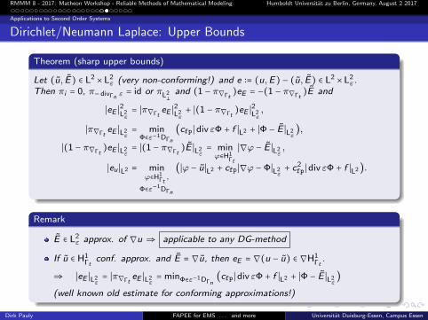
Theorem (sharp upper bounds)
Let (u, E) ∈ L2 ×L2ε (very non-conforming!) and e ∶= (u,E) − (u, E) ∈ L2 ×L2
ε.Then πi = 0, π− divΓn ε
= id or πL2
and (1 − π∇Γt)eE = −(1 − π∇Γt
)E and
∣eE ∣2L2ε= ∣π∇Γt
eE ∣2L2ε+ ∣(1 − π∇Γt
)eE ∣2L2ε,
∣π∇ΓteE ∣L2
ε= min
Φ∈ε−1DΓn
(cfp∣div εΦ + f ∣L2 + ∣Φ − E ∣L2ε),
∣(1 − π∇Γt)eE ∣L2
ε= ∣(1 − π∇Γt
)E ∣L2ε= minϕ∈H1
Γt
∣∇ϕ − E ∣L2ε,
∣eu ∣L2 = minϕ∈H1
Γt,
Φ∈ε−1DΓn
(∣ϕ − u∣L2 + cfp∣∇ϕ −Φ∣L2ε+ c2
fp∣div εΦ + f ∣L2).
Remark
E ∈ L2ε approx. of ∇u ⇒ applicable to any DG-method
If u ∈ H1Γt
conf. approx. and E = ∇u, then eE = ∇(u − u) ∈ ∇H1Γt
.
⇒ ∣eE ∣L2ε= ∣π∇Γt
eE ∣L2ε= minΦ∈ε−1DΓn
(cfp∣div εΦ + f ∣L2 + ∣Φ − E ∣L2ε)
(well known old estimate for conforming approximations!)
Dirk Pauly FAPEE for EMS . . . and more Universitat Duisburg-Essen, Campus Essen

RMMM 8 - 2017: Matheon Workshop - Reliable Methods of Mathematical Modeling Humboldt Universitat zu Berlin, Germany, August 2 2017
More Applications
More First and Second Order Systems (FOS & SOS)
Ω ⊂ R3 bounded weak Lipschitz domain
Electro/Magneto-Static Maxwell with mixed boundary conditions∇-rot-div-complex (symmetry!, de Rham complex):
0 or Rιπ
L2∇Γt
− divΓn εL2ε
rotΓt
ε−1 rotΓn
L2divΓt
−∇Γn
L2 πι
R or 0
related fos
∇Γtu = A in Ω ∣ rotΓt
E = J in Ω ∣ divΓtH = k in Ω ∣ πv = b in Ω
πu = a in Ω ∣ − divΓn εE = j in Ω ∣ ε−1
rotΓn H = K in Ω ∣ −∇Γn v = B in Ω
related sos
− divΓn ε∇Γtu = j in Ω ∣ ε
−1rotΓn rotΓt
E = K in Ω ∣ −∇Γn divΓtH = B in Ω
πu = a in Ω ∣ − divΓn εE = j in Ω ∣ ε−1
rotΓn H = K in Ω
corresponding compact embeddings:
D(∇Γt) ∩ D(π) = D(∇Γt
) = H1Γt L
2(Rellich’s selection theorem)
D(rotΓt) ∩D(− divΓn ε) = RΓt
∩ ε−1
DΓn L2ε (Weck’s selection theorem)
D(divΓt) ∩ D(ε
−1rotΓn ) = DΓt
∩ RΓn L2
(Weck’s selection theorem)
D(∇Γn ) ∩ D(π) = D(∇Γn ) = H1Γn L
2(Rellich’s selection theorem)
Weck’s selection theorem for weak Lip. dom. and mixed bc: Bauer/P./Schomburg (’16)
Dirk Pauly FAPEE for EMS . . . and more Universitat Duisburg-Essen, Campus Essen

RMMM 8 - 2017: Matheon Workshop - Reliable Methods of Mathematical Modeling Humboldt Universitat zu Berlin, Germany, August 2 2017
More Applications
More First and Second Order Systems (FOS & SOS)
Ω ⊂ RN bd w. Lip. dom. or Ω Riemannian manifold with cpt cl. and Lip. boundary Γ
Generalized Electro/Magneto-Static Maxwell with mixed boundary conditionsd-d-complex (symmetry!, de Rham complex):
0 or Rιπ
L2,0d0
Γt
− δ1Γn
L2,1d1
Γt
− δ2Γn
. . .dq
Γt
− δq+1Γn
. . .dN−1
Γt
− δNΓn
L2,N πι
R or 0
related fos
dqΓt
E = F in Ω
− δqΓn
E = G in Ω
related sos
− δq+1Γn
dqΓt
E = F in Ω
− δqΓn
E = G in Ω
includes: EMS rot / div, Laplacian, rot rot, and more. . .corresponding compact embeddings:
D(dqΓt) ∩ D(δ
qΓn) L
2,q(Weck’s selection theorems)
Weck’s selection theorem for Lip. manifolds and mixed bc: Bauer/P./Schomburg (’17)
Dirk Pauly FAPEE for EMS . . . and more Universitat Duisburg-Essen, Campus Essen

RMMM 8 - 2017: Matheon Workshop - Reliable Methods of Mathematical Modeling Humboldt Universitat zu Berlin, Germany, August 2 2017
More Applications
More First and Second Order Systems (FOS & SOS)
Ω ⊂ R3 bounded strong Lipschitz domain
Elasticitysym∇-Rot Rot⊺S -DivS-complex (symmetry!):
0ιπ
L2sym∇Γ
−DivSL2S
Rot Rot⊺S,Γ
Rot Rot⊺S
L2S
DivS,Γ
− sym∇
L2 πι
RM
related fos (Rot Rot⊺S,Γ, Rot Rot⊺S first order operators!)
sym∇Γv = M in Ω ∣ Rot Rot⊺S,Γ M = F in Ω ∣ DivS,Γ N = g in Ω ∣ πv = r in Ω
πv = 0 in Ω ∣ −DivS M = f in Ω ∣ Rot Rot⊺S N = G in Ω ∣ − sym∇v = M in Ω
related sos (Rot Rot⊺S Rot Rot⊺S,Γ second order operator!)
−DivS sym∇Γv = f in Ω ∣ Rot Rot⊺S Rot Rot
⊺S,Γ M = G in Ω ∣ − sym∇DivS,Γ N = M in Ω
πv = 0 in Ω ∣ −DivS M = f in Ω ∣ Rot Rot⊺S N = G in Ω
corresponding compact embeddings:
D(sym∇Γ) ∩ D(π) = D(∇Γ) = H1Γ L
2(Rellich’s selection theorem and Korn ineq.)
D(Rot Rot⊺S,Γ) ∩ D(DivS) L
2S (new selection theorem)
D(DivS,Γ) ∩ D(Rot Rot⊺S ) L
2S (new selection theorem)
D(π) ∩ D(sym∇) = D(∇) = H1 L
2(Rellich’s selection theorem and Korn ineq.)
two new selection theorems for strong Lip. dom.: P./Zulehner (’17)
Dirk Pauly FAPEE for EMS . . . and more Universitat Duisburg-Essen, Campus Essen
RMMM 8 - 2017: Matheon Workshop - Reliable Methods of Mathematical Modeling Humboldt Universitat zu Berlin, Germany, August 2 2017
More Applications
More First and Second Order Systems (FOS & SOS)
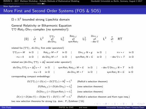
Ω ⊂ R3 bounded strong Lipschitz domain
General Relativity or Biharmonic Equation∇∇-RotS-DivT-complex (no symmetry!):
0ιπ
L2∇∇Γ
div DivSL2S
RotS,Γ
sym RotT
L2T
DivT,Γ
− dev∇
L2 πι
RT
related fos (∇∇Γ, div DivS first order operators!)
∇∇Γu = M in Ω ∣ RotS,Γ M = F in Ω ∣ DivT,Γ N = g in Ω ∣ πv = r in Ω
πu = 0 in Ω ∣ div DivS M = f in Ω ∣ sym RotT N = G in Ω ∣ − dev∇v = T in Ω
related sos (div DivS∇∇Γ = ∆2Γ second order operator!)
div DivS∇∇Γu = ∆2Γu = f in Ω ∣ sym RotT RotS,Γ M = G in Ω ∣ − dev∇DivT,Γ N = T in Ω
πu = 0 in Ω ∣ div DivS M = f in Ω ∣ sym RotT N = G in Ω
corresponding compact embeddings:
D(∇∇Γ) ∩ D(π) = D(∇∇Γ) = H2Γ L
2(Rellich’s selection theorem)
D(RotS,Γ) ∩ D(div DivS) L2S (new selection theorem)
D(DivT,Γ) ∩ D(sym RotT) L2T (new selection theorem)
D(π) ∩ D(dev∇) = D(dev∇) = D(∇) = H1 L
2(Rellich’s selection theorem and Korn type ineq.)
two new selection theorems for strong Lip. dom.: P./Zulehner (’16)
Dirk Pauly FAPEE for EMS . . . and more Universitat Duisburg-Essen, Campus Essen

RMMM 8 - 2017: Matheon Workshop - Reliable Methods of Mathematical Modeling Humboldt Universitat zu Berlin, Germany, August 2 2017
More Applications
There are More Complexes . . .
. . . the world is full of complexes. ;)
Hence: relaxing and enjoying complexes at
AANMPDE 10
10th Workshop on Analysis and Advanced Numerical Methodsfor Partial Differential Equations (not only) for Junior Scientists
https://www.uni-due.de/maxwell/aanmpde10
October 2-6, 2017 Paleochora, Crete, Greece
organizers: Ulrich Langer, Dirk Pauly, Sergey Repin
Dirk Pauly FAPEE for EMS . . . and more Universitat Duisburg-Essen, Campus Essen