FAKULTÄT FÜR INFORMATIKDER TECHNISCHEN UNIVERSITÄT MÜNCHEN

Master’s Thesis in Informatics

Development of a Co-Simulation frameworkto analyse attacks and their impact

on Smart Grids

Alexander Giehl

FAKULTÄT FÜR INFORMATIKDER TECHNISCHEN UNIVERSITÄT MÜNCHEN

Master’s Thesis in Informatics

Development of a Co-Simulation framework to analyseattacks and their impact on Smart Grids

Entwicklung einer Co-Simulationsumgebung zurAnalyse von Angriffen und deren Auswirkungen auf

Smart Grids

Author: Alexander GiehlSupervisor: Prof. Dr. Claudia EckertAdvisors: Dr. rer. nat. Christoph Krauß

Norbert Wiedermann, M.Sc.Dipl.-Inf. Thomas Kittel

Submission Date: July 15, 2013

I assure the single handed composition of this master’s thesis only supported by declaredressources.

Munich, July 15, 2013 Alexander Giehl

Abstract

Smart Grids are a new type of electrical grid combining traditional power networks withmodern information and communication networks. Smart Grids meet the challenges ofdepleting fossil fuels and increasing energy demand by introducing a larger portion of re-newable energy sources to the energy mix. Smart Grids utilize communication networksto provide high flexibility and reliability. For example, dynamic storage of energy genera-ted from weather-dependent sources is necessary. As a result, components of power andcommunication networks have become increasingly more interconnected.This trend has lead to computer networks previously closed off from the outside worldbeing connected to public networks. Security in those networks has been neglected duringtheir isolation from other communication networks. This has implications on the securityof supply since it creates new attack vectors for criminal individuals and organizationstrying to disrupt the stability of the energy supply for personal gain.In order to demonstrate how power networks can be affected by attacks propagated thoughthe underlying communication networks, we propose a security simulation framework.Existing simulation environments are integrated into a Communication and Power net-work Co-Simulation (CoPS). CoPS enables the definition of attacks on the data network ofSmart Grids, the simulation of these attacks and the study of their impact on the energydistribution. Further, CoPS aims at assessing the broader effects of those attacks and, the-refore, encompasses the domains private consumer and energy distribution.To show the feasibility of CoPS, two attacks are presented, one targeting the consumers inthe Smart Grid and one the distribution network itself. The results show, that an attackerwith access to the communication network is able to disrupt the energy distribution byforcing outages and therefore threatening the security of supply.

vii

Zusammenfassung

Smart Grids sind Energieinformationsnetze, die traditionelle Stromnetze mit modernerInformations- und Kommunikationstechnik (IKT) kombinieren. Smart Grids begegnen denProblemen, die sich aus schwindenden natürlichen Ressourcen und gleichzeitig steigen-dem Energiebedarf ergeben, indem sie eine Erhöhung des Anteils an erneuerbaren Energi-en im Energiemix forcieren. In einem Energieinformationsnetz werden IKT-Komponentenverwendet um hohe Flexibilität und Zuverlässigkeit zu gewährleisten, zum Beispiel ist dasZwischenspeichern von Energie, welche von wetterabhängigen Quellen stammt, nötig.Bisher sind Datennetze, wie sie im Energie erzeugenden Sektor eingesetzt werden, nichtan öffentliche Netze angeschlossen. Aufgrund dieser Trennung wurden, um Kosten zusparen, Sicherheitsvorkehrungen nur bedingt oder gar nicht umgesetzt. Zur weiteren Ko-stensenkung und Effizienzsteigerung werden diese isolierten Netze nun aber an öffentli-che Datennetze angebunden. Nachrüstungen im Bereich der Sicherheit fanden nicht stattoder wurden nur dürftig umgesetzt. Dies eröffnet neue Angriffsvektoren für kriminelleIndividuen und Organisationen, die versuchen die Stabilität des Stromnetzes zu beein-trächtigen.Um demonstrieren zu können, wie Stromnetze durch Angriffe auf die zugehörigen IKT-Netze betroffen sind, wird in dieser Arbeit ein Framework zur Simulation solcher Angriffeentwickelt. Dazu werden existierende Simulationsumgebungen für Strom- und Datennet-ze im Rahmen einer Co-Simulation integriert. Das Framework erlaubt die Definition vonAngriffen auf das Datennetz eines Smart Grids, die Simulation dieser Angriffe und dieAuswertung der Ergebnisse. Es werden dabei jeweils die Domänen Privatkunde und Ver-teilnetz innerhalb des Smart Grids berücksichtigt.Um die Anwendbarkeit von CoPS zu demonstrieren, werden zwei Angriffsszenarien vor-gestellt, wobei eines die Kunden im Smart Grid betrifft und eines das Verteilnetz. Die Er-gebnisse zeigen, dass ein Angreifer mit Zugriff auf die IKT-Infrastruktur in der Lage ist,die Energieversorgung empfindlich zu stören und dadurch die Versorgungssicherheit zugefährden.

ix

Danksagung

Für ihre Unterstützung bei meiner Masterarbeit möchte ich mich bei den folgenden Perso-nen herzlich bedanken:

Bei Frau Prof. Dr. Claudia Eckert, Leiterin der Fraunhofer-Einrichtung für Angewandteund Integrierte Sicherheit (AISEC), dafür, dass Sie mir die Möglichkeit einräumte, meineAbschlussarbeit an dem von Ihr geführten Einrichtung durchführen zu können.

Bei meinen Betreuern, Herrn Dr. rer. nat Christoph Krauß und Herrn Norbert Wieder-mann, M.Sc., für Ihre hilfreichen Anmerkungen und für Ihr konstruktives Feedback wäh-rend der gesamten Arbeit. Beiden möchte ich für das Lesen meiner Abschlussarbeit unddas kritische Korrekturlesen besonders danken.

Mein ganz besonderer Dank gilt meinen Eltern, die mich immer während meines gesam-ten Studiums unterstützt haben. Ohne Sie wäre diese Abschlussarbeit nicht möglich ge-wesen.

xi

Table of Contents

Abstract vii

Zusammenfassung ix

1 Introduction 11.1 Motivation . . . . . . . . . . . . . . . . . . . . . . . . . . . . . . . . . . . . . . 11.2 Problem Statement . . . . . . . . . . . . . . . . . . . . . . . . . . . . . . . . . 41.3 Structure of the Thesis . . . . . . . . . . . . . . . . . . . . . . . . . . . . . . . 5

2 Background 72.1 Smart Grids . . . . . . . . . . . . . . . . . . . . . . . . . . . . . . . . . . . . . 72.2 Simulation of Smart Grids . . . . . . . . . . . . . . . . . . . . . . . . . . . . . 10

2.2.1 Co-Simulation Primer . . . . . . . . . . . . . . . . . . . . . . . . . . . 102.2.2 Communication Network . . . . . . . . . . . . . . . . . . . . . . . . . 112.2.3 Power Network . . . . . . . . . . . . . . . . . . . . . . . . . . . . . . . 14

3 Related Work 173.1 Communication/Power Co-Simulation . . . . . . . . . . . . . . . . . . . . . 173.2 Security simulations for SCADA systems . . . . . . . . . . . . . . . . . . . . 193.3 Scope of the Thesis . . . . . . . . . . . . . . . . . . . . . . . . . . . . . . . . . 20

4 Concept 214.1 Co-Simulation Framework . . . . . . . . . . . . . . . . . . . . . . . . . . . . . 21

4.1.1 General Approaches . . . . . . . . . . . . . . . . . . . . . . . . . . . . 224.1.2 Custom Approaches . . . . . . . . . . . . . . . . . . . . . . . . . . . . 234.1.3 Discussion . . . . . . . . . . . . . . . . . . . . . . . . . . . . . . . . . . 27

4.2 Simulated Attacks . . . . . . . . . . . . . . . . . . . . . . . . . . . . . . . . . . 284.2.1 Shutdown Scenario . . . . . . . . . . . . . . . . . . . . . . . . . . . . . 294.2.2 Price Update Scenario . . . . . . . . . . . . . . . . . . . . . . . . . . . 31

5 Implementation 335.1 Co-Simulation Architecture Overview . . . . . . . . . . . . . . . . . . . . . . 335.2 Communication Network Model . . . . . . . . . . . . . . . . . . . . . . . . . 355.3 Power Network Model . . . . . . . . . . . . . . . . . . . . . . . . . . . . . . . 385.4 Integration . . . . . . . . . . . . . . . . . . . . . . . . . . . . . . . . . . . . . . 41

5.4.1 Communication . . . . . . . . . . . . . . . . . . . . . . . . . . . . . . . 415.4.2 Simulations . . . . . . . . . . . . . . . . . . . . . . . . . . . . . . . . . 435.4.3 GUI . . . . . . . . . . . . . . . . . . . . . . . . . . . . . . . . . . . . . . 47

xiii

Table of Contents

6 Simulation & Results 516.1 Experimental Setup . . . . . . . . . . . . . . . . . . . . . . . . . . . . . . . . . 516.2 Shutdown Scenario . . . . . . . . . . . . . . . . . . . . . . . . . . . . . . . . . 52

6.2.1 Communication Network Model . . . . . . . . . . . . . . . . . . . . . 526.2.2 Power Network Model . . . . . . . . . . . . . . . . . . . . . . . . . . . 536.2.3 Results . . . . . . . . . . . . . . . . . . . . . . . . . . . . . . . . . . . . 54

6.3 Price Update Scenario . . . . . . . . . . . . . . . . . . . . . . . . . . . . . . . 556.3.1 Communication Network Model . . . . . . . . . . . . . . . . . . . . . 556.3.2 Power Network Model . . . . . . . . . . . . . . . . . . . . . . . . . . . 566.3.3 Results . . . . . . . . . . . . . . . . . . . . . . . . . . . . . . . . . . . . 57

7 Conclusion & Future Work 617.1 Conclusion . . . . . . . . . . . . . . . . . . . . . . . . . . . . . . . . . . . . . . 617.2 Future Work . . . . . . . . . . . . . . . . . . . . . . . . . . . . . . . . . . . . . 62

7.2.1 Power Network Model . . . . . . . . . . . . . . . . . . . . . . . . . . . 627.2.2 Communication Network Model . . . . . . . . . . . . . . . . . . . . . 63

Appendix 67

Appendix A Naming Conventions for GridLAB-D 67

Appendix B How to use the Framework 69B.1 Installation of CoPS . . . . . . . . . . . . . . . . . . . . . . . . . . . . . . . . . 69B.2 Running the included simulations . . . . . . . . . . . . . . . . . . . . . . . . 69B.3 Adding new simulations . . . . . . . . . . . . . . . . . . . . . . . . . . . . . . 70

List of Figures 71

References 73

xiv

1 Introduction

This chapter provides an introduction to this thesis. The motivation for conducting thisthesis is given in Section 1.1. The problem statement is introduced in the subsequent Secti-on 1.2. The structure of the thesis is outlined in Section 1.3.

1.1 Motivation

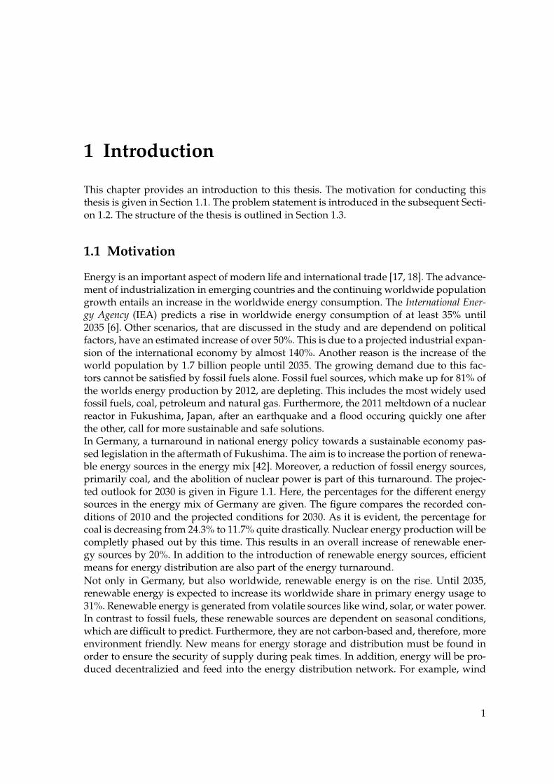
Energy is an important aspect of modern life and international trade [17, 18]. The advance-ment of industrialization in emerging countries and the continuing worldwide populationgrowth entails an increase in the worldwide energy consumption. The International Ener-gy Agency (IEA) predicts a rise in worldwide energy consumption of at least 35% until2035 [6]. Other scenarios, that are discussed in the study and are dependend on politicalfactors, have an estimated increase of over 50%. This is due to a projected industrial expan-sion of the international economy by almost 140%. Another reason is the increase of theworld population by 1.7 billion people until 2035. The growing demand due to this fac-tors cannot be satisfied by fossil fuels alone. Fossil fuel sources, which make up for 81% ofthe worlds energy production by 2012, are depleting. This includes the most widely usedfossil fuels, coal, petroleum and natural gas. Furthermore, the 2011 meltdown of a nuclearreactor in Fukushima, Japan, after an earthquake and a flood occuring quickly one afterthe other, call for more sustainable and safe solutions.In Germany, a turnaround in national energy policy towards a sustainable economy pas-sed legislation in the aftermath of Fukushima. The aim is to increase the portion of renewa-ble energy sources in the energy mix [42]. Moreover, a reduction of fossil energy sources,primarily coal, and the abolition of nuclear power is part of this turnaround. The projec-ted outlook for 2030 is given in Figure 1.1. Here, the percentages for the different energysources in the energy mix of Germany are given. The figure compares the recorded con-ditions of 2010 and the projected conditions for 2030. As it is evident, the percentage forcoal is decreasing from 24.3% to 11.7% quite drastically. Nuclear energy production will becompletly phased out by this time. This results in an overall increase of renewable ener-gy sources by 20%. In addition to the introduction of renewable energy sources, efficientmeans for energy distribution are also part of the energy turnaround.Not only in Germany, but also worldwide, renewable energy is on the rise. Until 2035,renewable energy is expected to increase its worldwide share in primary energy usage to31%. Renewable energy is generated from volatile sources like wind, solar, or water power.In contrast to fossil fuels, these renewable sources are dependent on seasonal conditions,which are difficult to predict. Furthermore, they are not carbon-based and, therefore, moreenvironment friendly. New means for energy storage and distribution must be found inorder to ensure the security of supply during peak times. In addition, energy will be pro-duced decentralizied and feed into the energy distribution network. For example, wind

1

1 Introduction

Petroluem Coal Natural Gas Renewable Nuclear Other

2010 33,80% 24,30% 20,60% 10,80% 8,80% 1,70%

2030 30,50% 11,70% 24% 30,80% 0% 3%

0,00%

5,00%

10,00%

15,00%

20,00%

25,00%

30,00%

35,00%

40,00%

Pe

rce

nta

ge

Figure 1.1: Estimated change in the energy mix of Germany until 2030 (Source: [19]).

energy produced at offshore parks in the North Sea needs to be transported to the southof Germany and solar energy vice versa.For the reasons stated in this section, the energy sector is subject to great change. A suitableinfrastructure for information and communication technologies is key in this development.Smart control is necessary to counteract or prevent fluctuation in energy generation fromrenewable sources. Moreover, efficient ways for energy storage, distribution, and trans-portation are needed to ensure power is available when needed, for example during peaktimes or in heavily industrialized areas. For this to be possible, more detailed collection ofdata, which reflects energy consumption and demand, then currently performed is neces-sary. Furthermore, this data needs to be exchanged between the different actors found inthe energy sector. This combination of energy and information technology is referred to asSmart Grid.Figure 1.2 shows a conceptional illustration of a Smart Grid. The decentralized architectureis shown as well as the interactions between the different components. Localized energyproduction is shown prominently in the figure. On the left hand side, a wind farm is il-lustrated. The produced energy is stored in large batteries and fed into the grid duringtimes of high demand. The same is true for energy produced with solar panels, which areeither installed on rooftops of private residences or on top of office buildings. Traditionalenergy producers are seen on the bottom of the figure. An industrial and central powerplant, which are integrated into the grid, are shown. Sensors and actuators are present inthe entire Smart Grid. On the one hand, they manage the efficient distribution of energyin the grid. On the other hand, they are also responsible for detection of disturbances inthe grid. One such disturbance is shown on the right hand side. In the scenario shownhere, the disturbance is due to natural causes (lightning). However, also deliberate attackson the Smart Grid could led to disturbances and outages. Since a Smart Grid is a criticalinfrastructure, guaranteeing the security of supply is essential and security in Smart Gridsis of paramount interest.

2

1.1 Motivation

Figure 1.2: Conceptual structure of a Smart Grid (Source: [17]).

Attacks on public infrastructure via the communication channels have occurred in the past.An example of such an attack is the W32.Stuxnet worm, that emerged in 2010 [8]. The net-works targeted in the affected plant were not even connected to the Internet. It is assumed,that the alleged attackers used USB devices to plant the worm inside the enterprise net-work of the target facility. The infected USB devices were transported into the facility byunsuspecting employees, who used the devices also on their private home computers. Theinitial infection occurred on these private machines, which were connected to the Internet.Other examples of attacks on public infrastructure are Maroochy Shire, Australia, and OakHarbor, USA [44]. In Maroochy Shire, the local sewage treatment plant was the target of acyber attack. As a consequence, 800 000 liters of untreated water were released in the eco-system, which caused severe damage to the local flora and fauna. The Davis-Besse nuclearpower plant in Oak Harbor was attacked by the SQL slammer worm and left without afunctioning safety monitoring system for almost five hours.

3

1 Introduction

1.2 Problem Statement

Section 1.1 already mentioned the increasing interconnection of data and energy networksand the reasons for this development. On the one hand, the expected benefits are of eco-nomical nature. Energy customers, this includes private as well as industrial customers,should be enabled to obtain energy when the price for it is currently low. This could redu-ce the costs for energy intensive operations. For example, if it is of no concern to a privatecustomer at what time a certain household appliance is started, then the machine could bestarted when the price for energy becomes cheap. The incentive for the customer wouldbe reduction of energy costs. On the other hand, also fluctuations, as they are caused byrenewable energy sources, could be compensated this way. For example, a cold storagefacility could be operated at full power when a large supply of energy is available. Whenthe facility is cooled down sufficiently, it could be disabled for a certain amount of timeand, therefore, save energy during that time. In addition to the benefits stated above, theGerman turnaround in energy policy calls for a dynamic solution to manage energy distri-bution. Data networks and information processing techniques are well-suited to meet thischallenge.The communication networks used in industrial production, that are also used in ener-gy generation and distribution, are currently isolated from other networks. In the processof introducing Smart Grids, these previously closed networks are connected. They canbe connected using public networks to exchange messages between each other. In SmartGrids, it is necessary to facilitate communication between the different parts of the grid, forexample for sending price notifications. However, this introduces new attack vectors sincethose systems were originally designed to be closed-off and small effort was invested insecurity mechanisms. Successfully executed attacks on even one component in the newlyformed network have the risk of cascading through the entire grid and are, therefore, af-fecting large portions of the entire structure. Examples for attack vectors are (Distributed)Denial-of-Service, Trojans, Address Manipulation, or Zero Day Exploits.Studying the effects of such attacks are of paramount interest since Smart Grids are a criti-cal part of the public infrastructure. However, conducting experiments on the actual publicenergy supply is difficult. In addition, the costs for those experiments would be enormous.Especially in the context of security, experiments on public infrastructure are not feasible.The risk of causing damage to the grid is not to be disregarded. Furthermore, it may bedifficult to get acceptance for experiments on public infrastructure in the general popula-tion. In particular, the people in the areas affected by the experiments might initially notapprove of them.An alternative approach is to conduct the tests inside s simulation by using a model of theactual system. This enables the examination of attack vectors without conducting experi-ments in real world infrastructure. By using a reasonable complex model of the Smart Grid,the results of an attack can be investigated and conclusions can be drawn from the results.At the moment, no simulators for Smart Grids exist, that encompass the data and the ener-gy network. In particular, no security simulators for Smart Grids exist, that take a widerportion of the grid into account. For this reason, existing tools for simulating either data orenergy networks must be combined together towards a joint simulation, a co-simulation.Such a framework, that enables security studies on Smart Grids, is developed in this thesis.

4

1.3 Structure of the Thesis

1.3 Structure of the Thesis

The thesis is structured as follows: Chapter 2 provides background information on SmartGrids and the simulation of Smart Grids. Related work for the thesis is discussed in thesubsequent Chapter 3. The scope of this thesis is given at the end of the chapter. The de-veloped concept of the security framework is presented in Chapter 4. The conceptual ap-proach for integration of communication and power network within a co-simulation isexplained. The attack vectors for two security relevant scenarios are derived in this chap-ter as well. A reference implementation of the developed framework concept is describedin Chapter 5. The implementation of the attack vectors is covered in Chapter 6. The resultsfor the simulated attacks are given subsequently. Conclusions from the presented resultsare drawn in Chapter 7. An outlook on future work is is given at the end of the chapter.

5

2 Background

This chapter gives a theoretical overview about Smart Grids and the simulation of them.Structure and components of Smart Grids, and also SCADA systems, are covered in Sec-tion 2.1 in an more abstract way compared to Chapter 1. The simulation of these SmartGrids with current simulation environments is discussed in Section 2.2.

2.1 Smart Grids

There is no strict definition on how to structure the construction of Smart Grids since theyare in the progress of coming into existence. Therefore, this section provides a generaloverview of the structure and components of future Smart Grids. Furthermore, securityconsiderations in regard to Smart Grids are introduced.Smart Grids are characterized by their decentralized architecture [13]. A variety of hete-rogeneous components, which are currently found in the traditional energy supply sector,are linked to one and another to form an interconnected structure. Communication bet-ween these components occurs on wired or wireless channels, for example UMTS, Wi-Fi,or Powerline. The different networking technologies are combined together via the Inter-net to form an integrated structure. This structure is referred to as Smart Grid. It includes,among others, autonomous components acting as digital meters, called smart meter. Com-munication between different components might involve different protocols and might,therefore, require specialized gateway devices translating between protocols [17]. In addi-tion to the technical components, economical processes are integrated into the Smart Gridas well, making it a complex and critical part of the public infrastructure.In the energy sector, but also in other industrial applications, Supervisory Control and DataAcquisition (SCADA) systems are commonly used. These systems monitor industrial pro-cesses and are IT-based. An overview about the general architecture of SCADA systems isgiven in Figure 2.1. The control station is in charge of the industrial processes to be mo-nitored. Inside of the control station, work stations used by the operators managing thesystems are located [28]. These stations provide a Human-Machine Interface (HMI) to theoperators. Also, one Master Terminal Unit (MTU) is found at the control station. The MTUis responsible for the communication to the field devices at the remote sites. The field de-vices are either Remote Terminal Units (RTU) or Programmable Logic Controls (PLC). Theycarry out identical tasks, i.e., acquisition of data by sensor readings. The collected data iscommunicated to the MTU at the control station as required via a combination of variouswired and wireless channels. Based on the sensor readings, the MTU enacts controllingactions for the process. If some action is required, the MTU sends a message containing in-structions back to the respective field device. The field device in term enacts the specifiedactions by the actuators for the technical system.

7

2 Background

MTU

Control Station

RTU/PLCRTU/PLC

Control Station Local LAN

HMI

Remote Sites

System System

ActuatorSensor ActuatorSensor

Wired

Wireless

Sensor data

Control commands

Communication channels:

HMI

Operator

read

send

send

send

send

send

read

send

Figure 2.1: Conceptual view of SCADA system architecture.

8

2.1 Smart Grids

As already indicated, Smart Grids are a critical part of the public infrastructure, meaningconsiderations about their security are of paramount importance. SCADA systems, forexample used in power plants, were previously closed off from public communicationnetworks. Therefore, security was neglected due to performance considerations and con-venience. Real-time capabilities are important for SCADA systems and security checks,for example packet filtering, would reduce performance. Also, in case of an emergency itis desired, that the operator is able to get immediate access to the controlled system wi-thout further access control. Passwords, if they are used at all, are short and known by allteam members.

Energy Distribution

Maintenance

Customer

InternetDevice

AppliancesSmartMeter

GatewayCustomer Network

Service

Market

LocalNetwork

FieldDevice

Internal Network

SCADA Internet

Decentralized Energy

Generation Decentral Energy

Generation

Communication Link

Energy Generation

EnergyTransmission

NetworkDomain

Component

Figure 2.2: Simplified domains and connections among them (Source (updated): [18]).

The reasons stated here have made SCADA systems a security concern [18]. For securitystudies, the Smart Grid has been divided into different domains as shown in Figure 2.2.The domains typically are energy generation, energy transmission, energy distribution, custo-mer, market, maintenance, and service. Especially the domains energy distribution and custo-mer are of particular interest for studying security in Smart Grids, since they are subjectof major change. The reason for this is, that electrical energy will be generated by an in-creasing amount from renewable sources and, in addition to this, will be obtained from a

9

2 Background

multitude of producers. When the customer domain is taken into account, the main focusfor security relevant studies is on the subdomain of the private customer. In the following,the domain customer and the subdomain private customer will be used interchangeable. Oneof the central component in this domain is the gateway, which allows real-time calculati-on of the customer’s energy demand. Also, a smart meter and an Internet-enabled deviceowned by the customer, e.g., a private PC, are an additional part of this domain. Thesecomponents are connected to the customer’s private network, which is in term connectedto the Internet. The customer, or consumer, employs devices using energy, e.g., householdappliances. Some customers also produce energy, for example with solar collectors. If suchenergy producers are present, the customer is also referred to as a producing consumeror prosumer. Both, consumer and prosumer, obtain their required energy from the distri-bution network. In addition, prosumer feed their locally produced energy into the grid.The domain energy distribution consists of distribution networks ranging from low voltage(120V) to middle voltage (max 20kV). The numbers refer to distribution networks insidethe USA (see Chapter 5.3). These networks are locally confined within 100 meters and se-veral few kilometers. They mostly supply low voltage household appliances located at thecustomer. The networks are maintained by the distribution system operator (DSO). Theenergy sold by the DSO is usually purchased from power plants, but the DSOs also pro-duce their own energy in a decentralized manner, for example in wind parks where windmills are operated by the DSOs. Currently, the distribution network is operated manual-ly but this is expected to change towards automated operation using SCADA technology.In the domains covered above, different actors take an active part. Those actors have dif-ferent tasks and responsibilities. The actors are referred to as roles. The DSO has alreadybeen introduced. Other roles are, for example, Metering Point Operator (MPO) and MeterService Provider (MSP). The MPO is operating the meter, whereas the MSP is reading outthe meter.

2.2 Simulation of Smart Grids

This section provides an overview about the simulation of Smart Grids. Section 2.2.1 mo-tivates the utilization of modeling and simulation techniques to be used for conductingresearch on Smart Grids. It also introduces the concept of co-simulation. Since Smart Gridscombine communication and power networks, existing simulation environments for bothare discussed in Section 2.2.2 and Section 2.2.3 respectively.

2.2.1 Co-Simulation Primer

In the context of this thesis, the term simulation is used to describe a virtual experiment [9].The experimental setup has been specified in the model together with the parameters forthe experiment. Simulation and modeling are always computer-based when discussed he-re. A simulator is any kind of framework or software package that allows modeling andsimulation. A communication simulator (CS) is a simulator for packet-based communicationnetworks, a power simulator (PS) is a simulator for electrical power networks.The simulation of electrical power networks offers some key benefits over conducting ex-periments on real world electrical structures. The electrical distribution network is covered

10

2.2 Simulation of Smart Grids

in this thesis. Using the actual distribution network for security penetration tests would re-quire to take the risk of power outages and damage to the components of the network. Thisis economically unfeasible. Also it might be difficult to gain acceptance for such projectsin the population affected by the tests. Even isolated tests of small substructures insidethe electrical network would suffer from this problem. A model of the electrical system tobe studied does not suffer from this drawbacks. Moreover, such models allow for a largerset of networks to be studied and the parameters of the experiment to be changed moreeasily. The inherent drawback of models is, that they only provide an approximation of themodeled object. Therefore, careful validation of the simulation’s results is necessary. Also,simulating complex models might require huge computational resources.A Smart Grid is a hybrid system [43]. It consists of a power and a communication net-work, both of which are complex systems for simulation on their own. Complex systemsoften need to be comprised as a hybrid system model since dedicated simulators for thesystem in question might not exist. The hybrid system model combines several partial mo-dels, which are specified with the respective simulator. For Smart Grids, at least CS anda PS are needed. The simulation of the partial models is conducted by the correspondingsimulators, however, a mediator is necessary for coordination efforts. This kind of simula-tion architecture is referred to as a co-simulation.Co-simulations were originally conceived to combine hardware/software (HW/SW) to-gether in a simulation environment [46, 41]. HW/SW co-simulations are also called hardware-in-the-loop simulations, since they introduce a physical component into the simulation run,for example a smart meter [44]. However, SW/SW co-simulation is also possible and isin fact easier to implement since HW/SW co-simulations require real-time ability. Anyco-simulation framework, however, will need a way to synchronize the internal clocks ofall simulators involved. This will be further discussed in Chapter 4, where the concep-tualization of a co-simulation framework capable of simulating Smart Grids is covered.Although the terms HW/SW and SW/SW imply, that only two simulators are used in a co-simulation, but several different simulators may be combined together to a co-simulation.

2.2.2 Communication Network

In this section, current frameworks for network simulation are introduced and discussed.Only freely available, widely used, open-source software packages are discussed. OPNETand NetSim are also widely used in research but were not considered due to the commer-cial nature of both products [36].

Network Simulator 2/3

The Network Simulator 2 (ns2) is an event-driven, discrete communication network simu-lator [39]. Its main area of application is the simulation of IP-based networks. Therefore, itoffers a rich library of different protocols and objects found inside such networks. Ns2 hasoriginally been developed for Unix platforms, however, it is usable on Windows machineswith Cygwin or comparable tools. It is licensed under the GNU General Public License 2.Ns2 has been written in C++ and it employs OTcl, an object-oriented extension to the ToolCommand Language (Tcl), as scripting language. Further, it uses the Network Animator(Nam), an animation tool for visualizing simulated networks.

11

2 Background

Figure 2.3 shows the simplified structure of ns2’s components and also illustrates the net-work modeling process. The network topology is described in an OTcl script. Each networkcomponent referred to in this file is defined in the Network Objects Library. This library ispart of ns2’s simulation kernel, which has been written in C++ for performance reasons.The corresponding objects are linked together for usage inside the simulation kernel. Thislinkage leads to a tight coupling between the topology description and the implementationof the objects and protocols. After specifying the network, the OTcl script is interpreted byan OTcl interpreter. The event scheduler is initialized and executed and then responsiblefor the progression of the simulation time. The running simulation and the results of thefinished simulation can be visualized using Nam.

C++ Simulation Library

Network Objects

Event Scheduler

Otcl Interpreter

Otcl Script Nam

Linkage

Figure 2.3: Structural view of ns2’s main components.

Ns2 is one of the most widely used network simulators in research and is well acceptedin academia. The reason for this is the early introduction of ns2 in 1997 and the constantdevelopment by the community. Ns2 uses obsolete software and its performance is notas good as the performance of more current network simulators [54]. Many tutorials andexamples have been published over the years, however, the overall documentation forns2 remains fragmented. To address the issues of ns2 and to provide a newer tool forresearchers, ns3 was developed [25]. Ns3 is not simply the next version of ns2, instead, itis a completely different simulator in respect to its architecture. It has a new software coreemphasizing modularity and scalability. The core is written in C++ as well and Pythonreplaces OTcl as scripting language. Development on ns3 began in 2006 and it has beenactively improved since then. Despite of this, ns3 has not been used widely in research bynow. Moreover, its capabilities currently cannot match those of ns2, making ns3 not yet areal alternative to ns2.

12

2.2 Simulation of Smart Grids

OMNeT++

OMNeT++ is a discrete event simulator for modeling communication networks [51]. It isC++-based, open source, and free for non-profit use. Version 4.2.2 of OMNeT++ is discus-sed here. Version 4.3 was released in April 2013 but a change to the newer version wasnot necessary since no features relevant for the work in progress have been added. Thesimulator ships with its own, customizable IDE, which is based on Eclipse. Also, it is welldocumented.By design, OMNeT++ has a modular architecture and is a simulator for packet-based net-works in general. This implies, that OMNeT++ can be, for example, used to study queuingproblems. This open architecture offers more possibilities for modeling but increases thelearning curve as well. The main usage of OMNeT++, however, is simulating communi-cation networks. The INET package of OMNeT++ contains all libraries necessary for buil-ding communication network models and running simulations with them. Several proto-cols, for example TCP, IPv4, IPv6, UDP, PPP, and Ethernet, are included [4]. The package isalso free for non-profit use and includes its own documentation. However, some chaptersin this documentation are unfinished in the manual for Version 2.1 of INET. The chaptersconcerned are 1.3, 2.4-2.10, 3.8, 3.9, 6, 7, 10, 13, 14, and 17. Relevant chapters explaining theusage of the INET framework and its most commonly employed features are fully docu-mented but for some modeling efforts it might be necessary to study the source code ofINET and the included demo projects in order to get the desired information.One important property of OMNeT++ is its ability to develop hierarchical models mea-ning that modeled objects can be subclasses of other objects or being subclassed themsel-ves. This allows models developed with OMNeT++ to be well structured and reused easi-ly. OMNeT++ further introduces the possibility of graphical modeling with the NetworkDescription Language (NED) and its corresponding editor. Figure 2.4 shows the NED edi-tor during design time, the depicted network is part of the broadcast demo included inINET. The components selected from the objects palette on the right are placed via dragand drop in the editor and are connected to each other by clicking. Some simple modelscould be completely described with the NED editor without the need for adding sourcecode [44]. The model descriptions could also be changed without further recompilation.This introduces a plug and play behavior to OMNeT++.

Figure 2.4: OMNeT++’s NED Editor showing a simple UDP-based network.

13

2 Background

OMNeT++ distinguishes between experiment, model and simulation [52]. Parameters canbe specified in configuration files. By default, the configuration file is called omnetpp.ini.The parameters affect the properties of different network objects during runtime, for ex-ample the number of hosts connected to a router. When the simulation is started, OM-NeT++ loads the parameters from the configuration file and determines the model for thesimulation. The parametrized network is then simulated. With this distinction, it is possi-ble to allow varying the parameters of experiments with the experimental setup remainingunchanged.

2.2.3 Power Network

This section gives more details on the simulation of power networks for Smart Grids. Exi-sting power network simulators can be modified to simulate Smart Grids [37, 23]. Al-so, isolated models of specific components within Smart Grid, like windmills, are usedin research [44]. However, using a simulator developed specifically for the simulation ofpower networks as they occur in Smart Grids requires no modifications. Moreover, it al-lows a comprehensive study of effects on the whole Smart Grid power structure [10, 31].GridLAB-D is such a simulator, in fact it is the only open-source simulator for the studyof power networks specific to Smart Grids [12]. For this reason, it is the only simulatorcovered in this section. Other commercial simulators for power networks, that have be-en successfully used in co-simulations, are PSLF and PowerWorld. Also Matlab/Simulinkand Modelica models of power components and small networks are employable.The core algorithm of GridLAB-D is designed to handle a multitude of independent de-vices. GridLAB-D utilizes agent-based modeling, meaning it represents processes as dy-namic systems of interacting agents. These agents represent a variety of different actorsinside a Smart Grid scenario, for example customers trying to minimize the price for ener-gy. As of May 2013, the current stable version of GridLAB-D is Version 2.2, Version 3.0 isin development and scheduled for release in the 3rd quarter of 2013.So far, GridLAB-D has found some use in research. It is actively developed and supported.Documentation can be found in the official wiki, help with occurring problems is providedin the technical support forum, which is frequented by the developers [29]. A drawback isthe missing IDE and the lack of graphical support during modeling. Modeling typically isconducted by using a text editor. The simulation is then started via a command line tool.It has been announced, that Version 3.0 will include a graphical editor. Visualization of thesimulated structure during runtime is not possible by now as well. Also, the experimen-tal nature of the generators library may result in problems during modeling. In addition,GridLAB-D only supports power networks as they are found in the USA. This is due tothe nature of GridLAB-D’s funding by the U.S. Department of Energy.

14

2.2 Simulation of Smart Grids

GridLAB-D ships with different libraries containing various models for components ofSmart Grids. In the following, an overview about the modules included in GridLAB-D 2.2is given.

• PowerflowDistribution network model can consist of transformers, regulators, fuses, substati-ons, capacitors, switches, overhead lines, and underground lines. Available solvermethods for the power flow equations are Forward-Backward-Sweep (FBS), Gauss-Seidel (GS), and Newton-Raphson (NR).

• ResidentialDetailed model for a single family residence with several household appliances, forexample water heaters or dish washers. It represents the customer within the SmartGrid.

• ClimateAggregated weather data for several cities in the USA is included. The climate mo-dels can be used in any simulation affecting, for example, wind mills and solar col-lectors.

• Generators (experimental, community-developed)Officially not supported. Models for windmills, solar collectors, DC to AC inver-ters, diesel generators, and batteries are included. Most of the models are functional,however, undocumented bugs exist and documentation on the usage of these com-ponents is scarce.

• ReliabilityDefinitions and tools for reliability analyses in distribution systems based on theIEEE 1366-2003 standard [1]. Also opening and closing switches is made possible.

• TapeWrites the output of the simulation runs. Output is possible to file, to shared memoryor to picture using gnuplot. MySQL access is also possible. However, the correspon-ding library for MySQL support is only accessible to GridLAB-D developers andconsidered to be experimental.

• MarketWholesale market model enabling the placement of bids into auctions. This way,price development according to demand is simulated.

• Commercial (unvalidated)Models for commercial buildings. Currently, only small offices are included but fu-ture additions are planned.

• PLC (deprecated)Custom controller models allowing modelers to specify the behavior of componentsduring runtime. It will not be supported in Version 3.0.

15

3 Related Work

This chapter presents work related to the thesis. In Section 3.1, approaches for communi-cation and power networks co-simulation are discussed. The provided list makes no claimto completeness. A comprehensive summary is given in [36]. In Section 3.2, research aboutsecurity in SCADA systems is discussed. Here, only research employing modeling and si-mulation is taken into account. Furthermore, research of theoretical nature not providingexperimental results is omitted as well. The scope of this thesis is given in Section 3.3.

3.1 Communication/Power Co-Simulation

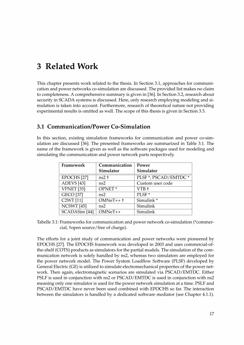
In this section, existing simulation frameworks for communication and power co-sim-ulation are discussed [36]. The presented frameworks are summarized in Table 3.1. Thename of the framework is given as well as the software packages used for modeling andsimulating the communication and power network parts respectively.

Framework Communication PowerSimulator Simulator

EPOCHS [27] ns2 † PLSF *, PSCAD/EMTDC *ADEVS [43] ns2 Custom user codeVPNET [35] OPNET * VTB †GECO [37] ns2 PLSF *C2WT [11] OMNeT++ † Simulink *NCSWT [45] ns2 SimulinkSCADASim [44] OMNeT++ Simulink

Tabelle 3.1: Frameworks for communication and power network co-simulation (*commer-cial, †open source/free of charge).

The efforts for a joint study of communication and power networks were pioneered byEPOCHS [27]. The EPOCHS framework was developed in 2003 and uses commercial-of-the-shelf (COTS) products as simulators for the partial models. The simulation of the com-munication network is solely handled by ns2, whereas two simulators are employed forthe power network model. The Power System Loadflow Software (PLSF) developed byGeneral Electric (GE) is utilized to simulate electromechanical properties of the power net-work. Then again, electromagnetic scenarios are simulated via PSCAD/EMTDC. EitherPSLF is used in conjunction with ns2 or PSCAD/EMTDC is used in conjunction with ns2meaning only one simulator is used for the power network simulation at a time. PSLF andPSCAD/EMTDC have never been used combined with EPOCHS so far. The interactionbetween the simulators is handled by a dedicated software mediator (see Chapter 4.1.1).

17

3 Related Work

EPOCHS has been used in research related to Special Protection Systems (SPS) (also calledRemedial Action Systems, RAS). These systems are designed to detect abnormal conditi-ons and to apply corrective actions if necessary. The communication occurring in a SPS isdifferent from the communication in SCADA systems since a SPS requires a rapid respon-se to the abnormal condition. A SCADA field device would communicate back to the MTUfirst and wait for further instructions.A similar approach to EPOCHS is ADEVS [43]. It uses the Discrete Event System Specifi-cation (DEVS), a formalism for building and simulating hybrid system models [47]. DEVShas been designed as a discrete event simulator, whereas the power network is a conti-nuous time simulation. As a consequence, it does not include a dedicated PS. This is themain drawback of DEVS since the user is required to provide custom code for the powernetwork components to be modeled. This code must then comply to the specification ofthe DEVS framework to be used successfully in ADEVS. In addition, commercial and non-commercial power network simulators do in general not comply to the DEVS specification.ADEVS was used to conduct experiments on how latency in communication networks af-fects power networks.Another co-simulation framework is VPNET [35]. It uses OPNET to simulate the commu-nication part and Virtual Test Bed (VTB) to simulate the electrical part. The data exchangebetween the two simulations is handled via a coordinator, which has been developed spe-cifically for VPNET. This co-simulation framework was designed for the study of powerelectronics rather then extensive power systems like Smart Grids and by that it might be,that VPNET will not scale properly when used to simulate a large scale power network. Inthe study conducted with VPNET, a DC-DC boost converter, a small electronic component,was simulated. The corresponding communication network consisted only of two nodesand was not the main focus of the performed experiments.A more recent framework is the Global Event-Driven Co-Simulation (GECO) [37]. GECOintroduces the novel approach of a global event queue, in which all events happening inthe simulation are stored. This approach provides high accuracy and scalability, a formalproof of the method is given in [36]. Like EPOCHS, GECO uses ns2 and PLSF. The si-mulators are combined via the global event queue written in the programming languagesC++ and Tcl, also used by ns2. GECO is used to study the energy transmission domain. Inparticular, fault detection schemes using distance relays (also called impedance relays) arethe focus of research. This kind of relays are able to detect short circuit faults and furtherprovide an estimate on the position the faults occurred. It is possible to integrate othercommunication and power simulators in GECO, however, this could be complicated sinceit will require modifications to the simulators and the framework.A simulation framework used more widely in research is the Command and Control Wind-Tunnel (C2WT) [11] and the Networked Control System Wind Tunnel (NCSWT), whichitself is based on C2WT [45]. C2WT is designed as a general purpose co-simulation plat-form enabling the integration of different simulators. Currently implemented communi-cation simulators are ns2 and OMNeT++, the power network is modeled with Simulink.Most of the research using C2WT/NCSWT is of military nature, especially in the field ofUnmanned Aerial Vehicles (UAV), but civilian research has been conducted as well (seeSection 3.2). C2WT requires several additional software packages to be functional.Looking at the communication network simulators employed in the research presented inthis chapter, ns2 is the most widely applied. The reason for this is the early introduction

18

3.2 Security simulations for SCADA systems

of ns2 in 1997 and the constant development by the community. The power simulatorsused in communication and electrical co-simulation are more differentiated. This is becau-se of the different applications for the various co-simulation frameworks. However, thesimulators employed have their commercial nature in common. Freely available tools forresearchers of power networks are in general not available. An exception is GridLAB-D(see Chapter 2.2.3).

3.2 Security simulations for SCADA systems

SCADASim is a network simulator developed for security studies in SCADA systems [44].It implements most of the components of SCADA systems as described in Section 2.1. Ef-fort was put into enabling SCADASim to run hardware-in-the-loop simulations. The hard-ware components described in [44] were simulated with MATLAB/Simulink. In the eva-luation of the framework, the authors showed the application of SCADASim in small scalescenarios related to Smart Grids. The smart meter of a residence is exposed to a Denial-of-Service (DoS) attack, which had negative effects on the availability of the smart meter. Agateway component is not present in the simulation. The second demonstrated scenarioshows a spoofing attack on a wind mill. The wind mill was taken offline by falsified ser-vice requests in the simulation. The main focus of SCADASim, however, is not on SmartGrids but rather on general SCADA systems as they are found in public infrastructure, forexample transportation or water treatment. The framework consists mostly of the imple-mentation of the communication network. The communication part was developed withVersion 3.1 of OMNeT++ and Version 1.99.5, or an earlier version, of OMNeT++’s INETpackage. SCADASim can be executed with this software configuration on modern Linuxdistributions. Since Version 2.0 of INET introduced major updates to the INET framework[3], a port of SCADASim would be necessary for using it. For this reason, SCADASim itselfis not adopted into our framework. However, SCADASim provided sample implementa-tions of several components, which has proven to be helpful during the initial steps ofdevelopment of the communication network models.Security analysis on SCADA systems is also conducted with the C2WT framework [11]. Amodel of a chemical plant with a SCADA network attached to it is simulated. The modeledSCADA system is a simplified version of the Tennessee Eastman Control Challenge Pro-blem, a realistic chemical process, that is used widely in process control studies. The che-mical process takes place in an isothermal fixed volume reactor, which is monitored andcontrolled by a SCADA system. The model for the chemical process was implementedwith Simulink, the communication was simulated with OMNeT++. The network modelconsists of a series of connected routers. No other components are present in the network.Sensors, actuators, and the MTU are represented by routers. In addition, several relay rou-ters are found in the network map. Various of these routers are the target of DistributedDoS (DDos) attacks. As with SCADASim, this study also focuses on the SCADA systembut does not take the broader aspects of the Smart Grid into account. In order to make OM-NeT++ comply to the specifications of C2WT, extensive modifications to OMNeT++ mustbe applied [7]. Furthermore, other software used by C2WT also needed to be extended.The presented research focused on small scale scenarios. Typically, a single SCADA systemwas used in the conducted experiments. The modeling of the communication has been the

19

3 Related Work

main priority, whereas the power portion of the system was simulated with dedicated mo-dels in Simulink.

3.3 Scope of the Thesis

As compared to the related work discussed here, this thesis focuses on the development ofa co-simulation framework for security studies in Smart Grids. Other existing co-simulationframeworks for Smart Grids have other research objectives, for example market research [10,31]. So far, security related studies have only been conducted on isolated structures, whe-re SCADA systems are employed. This thesis is going to encompass a broader context byincluding several SCADA systems at once, as they are found in different locations of theSmart Grid. The proposed simulator is a dedicated security simulator for the Smart Grid.The simulated attack vectors will, therefore, take place in different domains of the SmartGrid and will have effects on the other domains. The domains addressed by the propo-sed attacks are the energy distribution and customer domains. As illustrated in Table 3.1, atleast one simulator used in a given co-simulation framework is of a commercial nature.For the thesis, two open source simulators are be integrated together to a communicationand power co-simulation for the first time.

20

4 Concept

This chapter introduces our concept for the implementation of a co-simulation environ-ment with the properties described in Chapter 2.2.1 and Chapter 3.3. Section 4.1 givesan overview about different approaches for implementing co-simulations and categorizesthem according to their architecture. Their advantages and disadvantages are discussedand a concept for implementation is developed. The attacks to be simulated with this co-simulation are described in Section 4.2. Two attack vectors are presented, each of whichtargeting a different domain of the Smart Grid. The approach of the attacker is explainedand the expected results of the attack are discussed.

4.1 Co-Simulation Framework

In this section, the different approaches for implementation of a co-simulation frameworkare examined. They are categorized by their properties and compared to each other to-wards their feasibility for implementing the proposed communication and power networkco-simulation. The approaches discussed here are all used successfully in literature. Theyare described in detail in Chapter 3.

Co-Simulation(Communication &

Power Network)

General

Custom

(Time-Stepped)

HLA

Other

VPNET

DEVS

EPOCHS

C2WTNCSWT

Synchonous

Asynchronous

GECO

IRW

SCADASim

Rauchfuss

et al.

Figure 4.1: Categorization of existing co-simulation frameworks.

The derived categorization is summarized in Figure 4.1. The second layer from aboveshows the two main approaches found for implementing co-simulation frameworks, ge-neral approaches on the one hand and custom approaches on the other hand. Generalapproaches aim at developing a co-simulation independent from the simulators used forthe partial models. The simulators are considered to be interchangeable [11, 27, 47, 35].In custom approaches, the simulators for the partial models are typically chosen first andthe co-simulation is then developed to integrate these environments [37, 10, 55]. The third

21

4 Concept

layer further divides these approaches by their most important property. For the generalapproaches, this are the specifications their implementation is based on. The specificationis either an official standard or derived from individual research. The main distinguishingproperty for the custom approaches is their synchronization method. The two main pro-perties for each approach will be discussed further in the subsequent sections. The leafnodes, to be found in the bottom layer of Figure 4.1, list existing implementations for eachapproach and property.

4.1.1 General Approaches

The most commonly employed technique for implementing general approach co-simu-lations is covered in this section. Other techniques share the same basic ideas and are,therefore, not covered in detail.The High Level Architecture (HLA) is an effort for standardizing general approach imple-mentations [2]. The HLA standard aims at promoting the interoperability of computersimulations and their reusability in different contexts. The abstract co-simulation architec-ture for conducting simulations within the HLA framework is depicted in Figure 4.2. Inthe HLA topology, the partial models are referred to as federates. They are connected via adedicated software mediator, the Run-Time Infrastructure (RTI). Together, federates and RTIcomprise the simulation, the so-called federation. Inside the federation, the RTI is the centraland most crucial component. It is responsible for managing the communication betweenthe federates via a publish/subscribe mechanism. The federates are not strictly aware ofthe RTI. By that, each individual federate would assume, that communication with theother federates is possible directly. Moreover, the RTI keeps the internal clocks of each fe-derate synchronized with the global simulation time. Therefore, the RTI implements thetwo most important features for successfully conducting any co-simulation.

Federation

Run-Time Infrastructure

Federate 1 Federate 2 Federate n. . .Publish/SubscribeCommunication

Figure 4.2: HLA federation.

22

4.1 Co-Simulation Framework

The High Level Architecture itself is a specification rather than a software package andso an implementation of HLA is needed in order to use the standard. If a custom imple-mentation of a RTI is not possible, choosing an already existing RTI is an important de-sign consideration. Several commercial-of-the-shelf and open-source RTIs exist. Examplesfor commercial RTIs are Chronos RTI, HLA Direct, SimWare RTI, Openskies RTI and Mit-subishi ERTI. Open source RTIs are, among others, CERTI, GERTICO, Portico, Open HLAand OpenRTI. Especially Portico has found wide usage in research. Implementations of theHLA standard, that are using the Java-based Portico, are EPOCHS, C2WT and NCSWT (seeChapter 3.1).General approaches have the advantage of interchangeable partial models. This propertymakes them easier to modify and extend during and after implementation. Newer partialmodels developed with updated or different simulators can be implemented more simp-ly. However, specifications for general approach co-simulations need to provide a genericframework to encompass all possible types of simulators and software [26]. This generatesoverhead for the implementation and affects the runtime. Furthermore, it could requirethe modification of the simulators before they are integrated into the co-simulation. Thesemodifications might be necessary for the simulators to comply to the specifications of thegeneric HLA framework. Since HLA is quite extensive, implementations result in softwa-re packages with many classes and lines of code, which results in a steep learning curvefor the usage of those packages. An example for such a complex implementation of HLAis C2WT. Other general frameworks, like DEVS and VTB (see Section 3.1), which are notusing the HLA specification but rather own specifications, suffer from the same draw-backs.

4.1.2 Custom Approaches

Custom approaches follow the same kind of algorithm [10, 41]. They exchange informationat specific points in time during the simulation for sending messages between the simu-lators and synchronizing the internal clocks. Since the synchronization happens at certainsteps in time, custom approaches are also referred to as time-stepped approaches.Figure 4.3 illustrates the sequential flow during the execution of any time-stepped simu-lation. Before actually executing the co-simulation, the initial parameters for the partialmodels need to be set. These step contains mostly initializations but also loading time. Af-ter the initial parameters are set and the simulators have loaded the partial models, thesimulations are started within each simualtor and the first interval is entered in the co-simulation. Now, both simulators simulate their respective partial models using the provi-ded parameters until the pre-defined internal time is reached. It is checked, if the reachedtime is equal to the stop time for the entire co-simulation. If so, the co-simulation finis-hes. Otherwise, the simulation of the interval continues. If some events occurred duringthe time step, the parameters for one or all partial models are updated accordingly. Then,the simulation continues with the next interval. Note, that all co-simulation approachesdiscussed so far are inherently based on time steps. This is also true for the general ap-proaches, since the RTI, or the corresponding equivalents in other specifications, forwardtime internally with time steps as well [26].

23

4 Concept

set initial

parameters

start simulators

Begin

simulate next

interval

update

parameters

Finish

[end time reached]

[else]

[event(s) occured]

[else]

Figure 4.3: Time-stepped simulation run.

24

4.1 Co-Simulation Framework

The time-stepped methods can now be further divided into the following two categories,synchronous and asynchronous methods. In [41], the terminology symmetric and asymmetricis used to describe, if one simulator is controlled by another. In the course of this work, thefocus is put on message exchange for which the terms defined here are more fitting. Thedifferent terminologies are not to be confused with each other.

Synchronous Co-Simulation

In a synchronous co-simulation, both simulation environments execute their respectivepartial simulation models independent from one another. The message exchange, and alsothe clock synchronization, is conducted at specific points in time. The interval of the pointsdoes not necessarily need to be predefined but can change during the simulation. Howe-ver, the next synchronization point must be known. This means, that the simulation can, intheory, be executed in parallel, as already implied in Figure 4.3. In principle, messages canbe passed at any point in time, however, this generates more synchronization effort andis more difficult to handle. SCADASim in an example for a synchronous co-simulations[44]. The simulations that are executed within the framework are intended to be run inreal-time. For this purpose, the execution takes place in parallel. Therefore, SCADASim isclassified as a synchronous method. Another example would be the Integrated Retail andWholesale (IRW) project [10] (see Chapter 7.2).

Asynchronous Co-Simulation

Asynchronous methods are executed in a stop-and-go like scenario [41]. Figure 4.4 illustra-tes this scenario for a communication and power network co-simulation. First, the commu-nication network is simulated until a certain synchronization event occurs. Those events,for example, could be messages produced by the simulation. The CS is stopped and thePS is started. Note, that the PS in this scenario is “one step behind” the CS, meaning thesimulation of the power network needs to “catch up” to the communication network, i.e.,reach the same internal time as the CS. For this reason, the amount of time passed since thelast event and the current stop is simulated with the PS. This is where the synchronizationof the internal clocks happens. After the PS has finished, and if the end of the simulationis not reached, the simulation parameters are updated according to the event that causedthe CS to stop. The implications this event has on the PS will take effect in the followingsimulation run of the PS. According to [41], this is a asymmetric co-simulation, because thePS is controlled by the CS in this scenario. Another co-simulation framework is GECO [37].In GECO, the simulation is also controlled from the CS. This shows the continuing trendof the CS being in control of the entire co-simulation. It is also possible for the PS to be incontrol of the simulation and to reverse the order of execution, i.e., start with the PS andhave the CS follow. This is depended of the modeled system and the purpose for whichthe system is modeled. The approaches in literature leave the CS in control. This is due tothe fact, that they study the implications something has on the power network and not theimplications the power network has on something else.

25

4 Concept

Begin

simulate

communication

stop simulation

simulate power

update simulation

parameters

Finish

[else]

[end time reached]

[else]

[internal clocks sync'd]

[else]

[event occured]

Figure 4.4: Asynchronous execution of a time-stepped simulation run.

26

4.1 Co-Simulation Framework

4.1.3 Discussion

Each time-stepped co-simulation must find a trade off between performance and the ac-curacy of the simulation. Long intervals between synchronization points for synchronousco-simulations means reduced synchronization overhead. Therefore, the co-simulation isexecuted more fluently. However, a proper response to events in time gets more difficultthe longer the simulation runs uninterrupted, rendering the event “lost”. GECO’s globalevent queue was implemented to counteract this behavior [37]. Is the interval on the otherhand to narrow, the accuracy of the co-simulation is increased but the overall performan-ce suffers from it. For asynchronous co-simulations, the performance might suffer as wellif the co-simulation is stopped on every event. Choosing important messages and onlyreacting to them is key for making asynchronous co-simulations more accurate and over-all better performing than synchronous co-simulations. In addition, an asynchronous co-simulation is more easier to implement since parallelism is disregarded.As already indicated in Chapter 2.2.3, GridLAB-D is the best choice for modeling thepower network within the co-simulation. For the communication model, ns2 and OM-NeT++ are the best candidates (see Chapter 2.2.2). In comparison, OMNeT++ has moreadvantages than ns2 [44, 54, 15]. Those advantages are summarized in the following:

• Modular specification of modeled objects is possible.

• Hierarchical modeling is supported.

• OMNeT++ includes its own IDE, which is based on Eclipse.

• It is more suited for the simulation of larger networks.

• More efficient use of resources and, therefore, faster simulation runs.

• Clear distinction between model, simulation and experiment.

• Extensive up-to-date documentation, that is included in the distribution.

The main advantage of ns2 over OMNeT++ is, that ns2 is a dedicated network simulatorcontaining a rich library of protocols. However, modeling rarely used protocols is not inthe scope of this work since it focuses on TCP/IP networks, which are included in OM-NeT++. For this reasons, OMNeT++ our the choice for the CS. OMNeT++ is a discreteevent simulator, whereas GridLAB-D is a continuous time simulator, making the wholecommunication/power-co-simulation a hybrid system model [47].Several simulators have been integrated in HLA already [11, 45, 37] but so far GridLAB-Dhas not been. Integrating a new simulator into HLA can be a time consuming task. Also, fa-miliarizing oneself with the HLA framework and one of its implementation holds a steeplearning curve. Using time-stepped co-simulation approaches is in general more intuiti-ve and provides more freedom during development. For this reasons, the asynchronous,time-stepped co-simulation model, as depicted in Figure 4.4, is chosen as conceptional ap-proach for implementation of the Smart Grid security simulation framework.

27

4 Concept

4.2 Simulated Attacks

The structure and the components for future Smart Grids, as described in Chapter 2.1, areby no means fixed or final. Instead, they will likely change. Also, new attack vectors willarise in the future and existing ones are bound to change. For those reasons, the archi-tecture for the co-simulation proposed in Section 4.1 needs to be expandable and a widevariety of different attacks should be possible for simulation. This goal is achieved by se-lecting modular, widely used and actively developed open-source simulators.Due to the complexity of the simulated object, i.e., the Smart Grid, it is not feasible tolist all the potential attack scenarios at this point. Many of them are discussed in litera-ture [17, 13, 18]. In order to provide a proof of concept, two sample attack scenarios areselected and integrated in the co-simulation framework. Both scenarios encompass thedomains consumer and energy distribution but the domain targeted by the attacker is diffe-rent for each scenario. The results, however, will effect both domains.The first attack vector is presented in Section 4.2.1. Its main purpose is to provide an acces-sible demonstration of the security framework. It is also used as a testing scenario duringthe initial steps of implementation. In the scenario, the attacker targets the energy distributi-on domain and disrupts the security of supply by successfully performing the attack. Thisis achieved by taking components of the distribution network offline. The distribution net-work modeled for this scenario is simple and does not entail many different components.The second scenario, introduced in Section 4.2.2, shows the capability of the framework toconduct large scale simulations. It encompasses a much larger distribution network thenthe first attack. The distribution network is based on a model derived from real world dis-tribution infrastructure. The targets of this second attack are the residences of the customerdomain supplied by the power network. The scenario examines the effects changing de-mand from a multitude of customers has on the stability of the distribution network andthe security of supply.Power generation from renewable energy sources, for example by wind mills or solar col-lectors, is not included into the proposed scenarios. The reasons for this decision are statedmore explicitly in Section 5.3. In short, this is due to the experimental implementation ofthe respective modules in GridLAB-D. Leaving out components like solar collectors meansalso, that no prosumers are present in the attack scenarios. The customers are representedsolely by regular consumers, each of which with its own smart meter and gateway. Howe-ver, fitting models for prosumers and wind parks are implemented within the frameworkand could be used in other scenarios (see Section 5.2). It is assumed, that the attacker ineach scenario has the means to infiltrate the communication network since security vulne-rabilities for the Internet protocol stack have well been researched and are not the focusof this thesis [16]. The immediate aim for the presented scenarios is to create a sense ofawareness among stakeholders.

28

4.2 Simulated Attacks

4.2.1 Shutdown Scenario

This section describes the attack, that is executed on the domain distribution network. Forfurther reference, the scenario described here is referred to as the Shutdown (SH) scenario.Previously closed off control networks, which are, for example, part of the energy sup-ply, are connected to publicly accessible networks, e.g., the Internet, in an increasing num-ber [17]. Using already existing communication platforms and technologies for interconnec-tion of the networks is economically reasonable. Moreover, efficient interconnection of thesystems involved is easier to implement when the same family of protocols is employed.The family used in those scenarios is the popular and widespread TCP/IP protocol suite.This introduces those networks to the well-known security vulnerabilities of TCP/IP pro-tocols [16].Parts of the public infrastructure, for example power networks, are a primary target forcyber-terrorists, who are trying to disrupt the energy supply via forced blackouts. This isalso true for hostile nations, which might launch computer-based attacks as a preliminarystep of a conventional assault [33]. In order to reduce costs, components in power networksare accessible via remote maintenance interfaces. Therefore, physical presence of operatorsis not required for routine maintenance tasks. This results in an overall increase in efficien-cy and is a method of saving costs as well. This fact could, however, be the entry point foran attacker as well. The attacker could use falsified packets to request service operations,for example an emergency shutdown of the component, which would be transmitted incase of technical difficulties.Figure 4.5 shows the schematic diagram of the Shutdown Scenario. The components of theelectrical grid, substation and transformer, are located in the domain energy distribution onthe top of the figure. In this domain, the control station is located as well. The control stati-on is home to the MTU, an important component inside the Smart Grid. The attacker sendsa manipulated emergency shutdown request targeting one of the electrical components inthe grid to the MTU. It is assumed, that the attacker has the means to forge his authentica-tion sufficiently so no flags are raised. The request is then distributed from the MTU to therespective SCADA component at the receiving facility. This component will then in termperform the shutdown. As a result, the connected houses in the customer domain (on thebottom of Figure 4.5) suffer from a blackout since the energy supply is interrupted.This scenario demonstrates the need of increased security in all SCADA networks connect-ed to the Internet or other public networks. Only one vulnerable component endangers thestability of the entire grid. The effects are in the best case local but might easily have broa-der implications.The extensive effects even one failing component has on the power supply have been sho-wed by an accident on November 15, 2012 in Munich [50]. The outage was caused by asubstation going offline after an accidental explosion and affected consumers as well asthe public infrastructure. As a consequence of the outage, blackouts occurred in the partsof the urban area. Furthermore, the public transportation was affected, as four subway li-nes went out of service. The effects of this incident were noticeable as far as 50 kilometersaway. The results would be similar when the component has been shut down by a requestsince it only is required for the substation to go offline without warning.

29

4 Concept

Domain Energy Distribution

Domain Costumer

Control Station (MTU)

Attacker

0

Substation

Transformer

House 1

0Communicaton

Component

Electrical Component

Communicaton Channel

ElectricalConnection

Manipulated Package

BrokenConnection

House 2

. . .

Figure 4.5: Conceptual view of the Shutdown attack.

30

4.2 Simulated Attacks

4.2.2 Price Update Scenario

In this section, the attack vector executed on the domain costumer is presented. The scena-rio described here is referred to as the Price Update (PU) scenario.Smart meter and gateways are deployed as mass products and installed at customers’ pre-mises [17]. These smart meter are connected to the grid via gateways and communicatewith other components of the grid. It is assumed here, that the communication betweensmart meter and gateway occurs unfiltered. This makes them a prime target for large sca-le attacks. Naturally, the customer himself is a potential attacker. However, manipulationof one smart meter has no broader impact on the power network. Therefore, this parti-cular scenario is disregarded. Instead, the focus is on those attack vectors targeting manyor all smart meter in a local area. Smart meter offer the possibility for customers to linkup their energy demand to the current price for electrical energy in order to achieve costsavings [18]. This is reasonable in a number of scenarios. For example, when the pricefor energy is currently low, a device with high energy consumption is switched on. Theprice update notification is sent to the gateway via public communication channels. Fromthe gateway, the notification is then further transmitted to the smart meter. The gatewaycomponent is necessary for translating between the IP and SCADA protocol families. Bytransmitting the price update notifications via public communication infrastructure, thepackets containing the price information become vulnerable for manipulation, for exam-ple, through a man-in-the-middle (MITM) attack. Also, the packets could be generated byan attacker and sent to the meter eliminating the need for an initially established connecti-on between customer, Metering Point Operator (MPO), and Meter Service Provider (MSP).From MPO and MSP, the transmitted data could also be sent to the Distribution SystemOperator (DSO). This is the case examined closer in the PU scenario.Figure 4.6 shows the conceptual sequence of the attack. The attacker, which could be thesame as described in Section 4.2.1, sends manipulated price update notifications to thecustomers, who in turn change their energy demand, for example, by attaching differenthousehold appliances to the power network. It is expected, that these changes in demandwill affect the local distribution network and will lead to oscillations within the energysupply. This makes the energy network unstable, i.e., the frequency required for properoperation drops below 60 Hertz (Hz) [53]. Affected are all households in the local part ofthe grid targeted by the attack. In the PU scenario, the whole simulated grid will be the tar-get. Blackouts and brownouts, the initial stage of a blackout, are the result. Brownouts, forexample, cause lights to dim or appliances to shut down. Apart from this nuisance, brow-nouts also affect electrical motors and could damage them severely. Overall, this attackvector shows, that also the customer domain is a target for attacks if the communicationbetween the different actors of the Smart Grid is not secured sufficiently.

31

4 Concept

Domain Energy Distribution

Domain Costumer

Gateway Smart Meter

Control Station (MTU)

Attacker

0

Substation

Transformer

0Communicaton

Component

Electrical Component

Communicaton Channel

ElectricalConnection

Manipulated Package

Change in Demand

Appliance(s)

House

Figure 4.6: Conceptual view of the Price Update attack.

32

5 Implementation

This chapter describes the development and implementation of the Communication &Power Network Co-Simulation (CoPS) based on the concept described in Chapter 4. Anoverview about the architecture of CoPS is given in Section 5.1. The individual modelingprocesses of the communication and power network are discussed in Section 5.2 and Sec-tion 5.3 respectively. The development of a distributed .NET application for integration ofthe models is presented in detail in Section 5.4.

5.1 Co-Simulation Architecture Overview

This section introduces the overall structure of CoPS and its main components. Details ofthe implementation are spared intentionally and will be discussed in the following secti-ons. CoPS consists of the components shown in Figure 5.1. The naming of the componentsreflects the real namespaces and class names used for implementation. The package on toplabeled CoPS.Models.Power shows the relevant components of GridLAB-D used inside thesimulation. The power network model is executed via the gridlabd.exe command line inter-face and generates an output in the form of comma-separated values (CSV). On the bottomof Figure 5.1, the CoPS.Models.Comm package contains classes developed in OMNeT++. Ex-ternal messages are received via the NotificationReceiver class and passed throughto OMNeT++’s scheduler: the CoScheduler, which was specifically developed for CoPS.It propagates the messages through the network model until the results of the simulationare available. They are then communicated back via the NotificationSender class. Inbetween the two simulator packages, the .NET classes, which together are in control ofthe simulation, are depicted. A graphical user interface (GUI) is provided in the CoPS.GUInamespace. The GUI offers an interface for users to conduct simulations. Here, the user se-lects the simulation for execution and monitors the progress of the simulation. Moreover,a graphical representation of the simulated network is shown. Helper classes are foundinside the CoPS.Libs.Messages library. The commands of the user are sent to OMNeT++ viaa dedicated server application (CoPS.GUI.Server), which is designed to run in a distribu-ted, networked environment. For this reason, the communication happens via an interfacespecified in the CoPS.WCF.Contracts shared library. This adds a Service-Oriented Architec-ture (SOA) to the framework. Other packages with helper classes are the general purposeCoPS.Lib library and the GridLAB-D specific CoPS.Lib.Gridlabd library. The first containsthe ConsoleApp class for executing command line tools, for example gridlabd.exe, andthe CSVParser class for reading the simulation results. The other helper library containsa parser for the modeling language of GridLAB-D (GLMParser), which is used to readthe model’s structure in the beginning. During the course of the simulation, the model isupdated with the GLMGenerator and changes are written to the Power Network Model file.

33

5 Implementation

OMNeT++

.NET

GridLAB-D

CoPS.Lib.Gridlabd CoPS.Lib

CoPS.Models.Power

CoPS.GUI CoPS.GUI.Server

CSVParser ConsoleAppGLMGenerator GLMParser

CoPS.Lib.Messages

Power Network

Modelgridlabd.exeCSV Data

«interface»

CoPS.WCF.Contracts

CoPS.Models.Comm

NotificationReceiver CoScheduler NotificationSender

Figure 5.1: Components and packages of the communication and power network co-simulation.

34

5.2 Communication Network Model

5.2 Communication Network Model

Network components in OMNeT++ are described with the Network Description Langua-ge (see Chapter 2.2.2). With modules and channels to connect modules, two types of compo-nent exist [52]. Modules are further divided in simple modules and compound modules.Simple modules implement the behavior of certain components and are, therefore, respon-sible for all activity occurring in a model. Their behavior is defined by the user in C++source code files. Compound modules are containers for simple modules and may containany number of simple modules. The network model is comprised of the modules and theirconnections. In order to develop communication networks as they can be found in SmartGrids, new compound modules for SCADA components are implemented. The followi-ng components are taken into account [44, 28]: Remote Terminal Unit (RTU), Program-mable Logic Control (PLC), Master Terminal Unit (MTU), and Human-Machine Interface(HMI) (see Chapter 2.1). These SCADA components are derived from INET’s standardcomponents, meaning they are treated by the simulation kernel as if they were INET’sStandardHost component. The model includes support for the OSI stack and the pro-tocols TCP/IP as well as UDP and ICMP. Smart meters are represented by the RTU. RTUand PLC more and more take over the same tasks and are, therefore, modeled identicallybut are present as individual components [5]. Moreover, the components implement theINET application interface allowing dynamic binding of the C++ programs describing thebehavior of the modules [4]. These applications communicate with each other via simula-ted network packets and make decisions based on the packets they receive. Furthermore,they are responsible for the communication to the outside of the model (see Section 5.4).In addition to the components mentioned above, a gateway component is implementedinto the framework. The gateway can be located in the customer domain, where it is usedto relay communication to the smart meter [17]. The gateway can also be employed in theenergy distribution domain, where it can be found in the SCADA networks of, for example,wind parks. The gateway is a compound module, that consists of several simple modu-les. Figure 5.2 shows the gateway and its simple modules. The gateway is also derivedfrom the StandardHost and so INET’s implementation of the OSI stack is clearly visibleinside the TCP/IP connectivity group. The Data Link Layer is represented by the simplemodule labeled eth[0] on the bottom. Packets received at eth[0] are first passed to the Net-work Layer protocol and then to the Transport Layer protocol, where TCP/IP is used. TheApplication Layer implements the behavior of the gateway via user-defined C++ code. Atthis point, the C++ applications describing the component’s behavior are integrated intothe model. In contrast to the other SCADA components, the gateway implements morefunctionality. It separates the IP net (box TCP/IP connectivity) from the SCADA net (boxSCADA connectivity). Communication between those two components takes place inter-nally via a publish/subscribe mechanism, as indicated by the doted line. This is the mostefficient way to handle communication inside the model. To avoid congestions, the mes-sages passed from the IP net are put into a queue and are subsequently sent to anothercompound module, in this case the smart meter, which is connected to the Queue but isnot visible in the figure. The implementation of the Queue component is adopted from thePFSim project [20]. Other INET components visible in the Configuration box on the left sideare NotificationBoard, RoutingTable and InterfaceTable. These componentsare responsible for proper packet routing inside the simulation. The gateway component

35

5 Implementation

has not been included in previous SCADA security frameworks (see Chapter 3) makingsimulations with CoPS more sophisticated and detailed.

Figure 5.2: Gateway component of CoPS during runtime of a Price Update attack.

The compound modules are grouped together in subnets representing organizational unitsof the Smart Grid. The basic structure is adopted from the large IPv4 Network demo inclu-ded in INET. Figure 5.3 shows the hierarchical relation between the different subnets. Theleaf nodes in the bottom layer are the subnets, which are used inside the simulation. Eachindividual entity is represented by a subnet, e.g., if there are three consumers in the simula-tion, three LanConsumer must be present in the communication network model. The othersubnets are abstract base types from which the leaf nodes are derived. For representingcomponents of the distribution network, subnetworks for wind parks (LanWindpark) andsubstations (LanSubstation) exist. For the consumer domain (see Chapter 2.1), regular con-sumers (LanConsumer) and prosumers (LanProsumer) using solar collectors are included inCoPS. The control station (ControlStation), where the MTU is located, is the central compo-nent of the network responsible for controlling the field devices, PLC and RTU, which arepresent in the other four subnets. Communication network models built with CoPS use forthe most part these components.Models are always an approximation of the modeled entity since real world objects areinherently complex and require assumptions to reduce their complexity in order to derivea feasible model, that can be used in computer simulations. The assumptions for the dif-ferent SCADA and network components, that are made during modeling, are discussedat this point. The SCADA component models are based on their descriptions providedin Chapter 2.1. The communication in the modeled network uses TCP/IP. The modeledcomponents are capable of communication via UDP and ICMP as well, however, this is

36

5.2 Communication Network Model

not used in the modeled network. An exception is the link between gateway and smartmeter, which is not handled by the INET package but rather by the simple packet basedcommunication of OMNeT++ and a publish/subscribe mechanism. Specialized modelsfor PLC and RTU are present in the model library of CoPS but inside the simulations theyare treated as identical components. At any time, there is only one MTU present in the en-tire network. This emphasizes the single point of failure characteristic of these component[18].Network models are calculated based on statistical models and are not fixed. Therefore, itis necessary to run a large amount of experiments before conclusions can be drawn [26].It is possible to use a deterministic algorithm for the generation of random numbers inOMNeT++, the Mersenne Twister Random Number Generator (MT-RNG) [52]. Using adeterministic RNG ensures, that multiply simulations of the same model produce identi-cal results, i.e., making the experiments reproducible. Furthermore, no sample space needsto be generated and conclusions can be drawn from one simulation run. The RNG mustuse the same seed for calculation of the random numbers to ensure this properties. This isachieved by setting the seed-0-mt property in the configuration file to an arbitrary 32-bitvalue.

LanBase

LanPowerBase LanHome

ControlStationLanSubstation LanWindpark LanConsumer Lan Prosumer

Figure 5.3: Subnetworks implemented in CoPS.

37

5 Implementation

5.3 Power Network Model

The information provided in this section, if not noted otherwise, is taken from the officialGridLAB-D wiki and the technical support forum [29]. Names written in typescriptindicate classes or components of GridLAB-D.

Nodes

Entry PointMeterNodeTriplex MeterHouse

RegulatorParent/ChildOverhead LineUnderground LineTransformer

LegendLinks

1000 1200 11001101

1102

1103

1400

3000

Figure 5.4: Visualization of a simple GridLAB-D distribution feeder.

GridLAB-D offers the possibility to model distribution networks, which are also referredto as feeder. The relevant components are specified in the Powerflow module. All com-ponents are derived from the two base types Node and Link. Node objects are connectedvia Link objects. Together they compose the feeder model. Most of the components in afeeder have configuration objects, which are here not further discussed for simplicity. Fee-der typically vary significantly in their structure [48, 49]. The feeder modeled by GridLAB-D are identical in their basic composition, which makes them more accessible. Figure 5.4depicts the basic composition for a GridLAB-D feeder. The feeder shown in this figure isnot atomic per se, however, it shows a baseline model of a distribution network using mostof GridLAB-D’s Powerflow components. The visualization of the feeder is done with theRuby script Glm2Dot [14]. The numbers attached to each Node follow the naming con-ventions listed in Appendix A. The magenta node (numbered 1000) on the left representsthe interface to the energy transmission domain, which is seen as the local substation of thefeeder. The lavender circle (1200) next to it is a Meter, connected via a Regulator link(red line). The small black dots represent regular Node objects (1100-1103). 1100 is the pa-rent of 1200 as indicated by the thin black line. The nodes are then connected by a series oflinks: An OvergroundLine (blue), an UndergroundLine (brown) and a Transformer(green), which are all derived from the Link base object in GridLAB-D. The orange circle(1400) is the TriplexMeter, i.e., the smart meter, which connects a House (3000) fromthe Residential module to the feeder.

38

5.3 Power Network Model

Within the GridLAB-D distribution, a set of distribution test feeders (DTF) is included. ADTF is a generalized model of a distribution feeder, which is used for benchmarking andto provide comparable experiments [32]. The feeders included in GridLAB-D are chosenby statistical analyses based on the data of 575 US feeder models [48]. They are charac-terized by climate region and voltage. A total of 24 typical feeders were compiled fromthe base data. Using one of these DTFs has the advantage, that an already tested model isused, which results in less errors. However, the feeder reflect the conditions present in thecontinental USA and not in Germany. Also, most of these feeders are quite complex, mea-ning they consist of many components and their structure is not apparent by reviewingthe source code file. However, using Glm2Dot the structure is made visible easily. Parts ofthe feeder can be taken offline with Switch links using the Reliability module, whichreduces the overall complexity since only a part of the feeder is used. This benefits the mo-deling of smaller scenarios. House nodes are integrated in the feeder via connecting themto Meter objects, that are already present in any DTF.Similar to House nodes, wind mills and solar collectors can be integrated in a DTF. An offi-cial documentation is not provided because of the experimental status of the Generatorsmodule, however, examples demonstrating their usage can be found in the GridLAB-Drepository. Wind mills (windturb_dg) integrate like Houses over a Meter into the fee-der, whereas solar collectors (solar) require an AC/DC converter (inverter) betweenHouse and solar collector. Two different wind mills are modeled in GridLAB-D, a 1.65 MWVestas V82 turbine and a 2.5 MW GE turbine [21]. For testing purposes, the Generatorslibrary of GridLAB-D 2.2 and the nightly build from March 15, 2013 are used to integra-te Generators objects into a simple DTF. The modules are functional mostly, however,crashes occur randomly during simulation without any error report. For this reason, theobjects of the Generators library are not included in the demonstration models.As mentioned in Chapter 2.2.3, the Residential module contains models for differenthousehold appliances. In GridLAB-D 2.2, the only supported model for such an applianceis the WaterHeater. Other models, e.g., DishWashers, are included, however, duringdevelopment it was found, that these models might not be functional in any scenario.Therefore, only the WaterHeater appliance is used. Multiple household appliances arerepresented by multiple instances of WaterHeater objects attached to one residence.The results of the simulation are recorded by the Tape module, either via a Recorder or aMultiRecorder. This is done for individual objects and properties, for example the vol-tage at a certain Meter could be reported. The object’s name and the property are passedto the (Multi)Recorder via a string attribute. The size of the string is limited internallyby a 1024 byte buffer. All recorders inside a simulation use the same buffer, i.e., there isonly one buffer for each simulation. This has implications on large scale simulations sincenot all desired values can be extracted from the simulation. This is due to the fact that onlya limited number of string attributes can be stored in a string of 1024 characters length.For this reason, the different residences in a feeder are grouped together to streets for thepurposes of demonstration. One residence in this street is randomly selected as the repre-sentative for the entire street, because the voltage levels at the residences of a street aresimilar.

39

5 Implementation

For all GridLAB-D models developed within CoPS, the assumptions and conventions ma-de in the remainder must be used. They will be used by the .NET implementation for theindividual simulation.The entry point for every DTF, i.e., the part of the feeder from the transmission network in-terface to the beginning of DTF structure, is the same for all feeder models. The followingcomponents are connected to each other in the order mentioned: Regulator (1000), node(1100), meter (1200), node (1101), switch (1900), and node (1102). Furthermore, those com-ponents must have the number in brackets assigned as internal ID. Note, that the switch(1900) is optional. However, if it is needed inside the simulation it should be used at theposition indicated here. When the switch is located between the second and the third nodeof a feeder, the whole power network can be taken online or offline easily.The starting time of the internal clock is set to 00:00:00 on 2000-01-01. This is the earliesttime that can be specified in GridLAB-D and is set for convenience.It is possible to split model definitions over different files. However, one file must containthe entire structure of the network for proper parsing. Other non-structural objects, forexample configuration objects of schedules, can be stored in separate files. The model forthe power networks is split upon several files. GridLAB-D allows to include model files inother models similar to the #include directive of C/C++. This facilitates the reusabilityof different parts of the model in other scenarios. The main file used in CoPS is named mo-del.glm, the extension GLM is short for GridLAB-D Model. In this file, the structure of thenetwork is described (see Chapter 5.2). The configuration objects are listed in a separatefile, model-config.glm. Separating structure and configuration provides better clarity whenupdating the structure. The configuration file is the same for the two power network mo-dels. Definitions and global variables are further provided in the model-header.glm file. Forthe Price Update Scenario, an additional model file named model-schedules.glm is provided.In this file, the schedule for the demand of the water heaters, used to model any house-hold appliance, is defined. Schedules are used by GridLAB-D for computing values, thatchange over the course of a specific time period, for example over the course of a day.

40

5.4 Integration

5.4 Integration

This section explains the development of the framework in control of the co-simulation.The integration of the two simulation environments into this framework is covered in Sec-tion 5.4.1. The implementation of the simulations is discussed in Section 5.4.2. The GUI isshown in Section 5.4.3.

5.4.1 Communication

External applications can be integrated in OMNeT++ by using one of the following threetechniques [38, 44]. First, Source Code Integration, i.e., the modification of OMNeT++’ssource code, second, Shared Library Integration, where a library used by both, OMNeT++and the external application, is developed or, third, by Socket Connections. Here, com-monly used network protocols are employed for communication.In order to use the first variant, knowledge of OMNeT++’s implementation is required.The source code needs to be recompiled using the specified build environment. The ex-ternal application must be integrated into this environment, which limits the flexibilityduring development and design. Moreover, familiarizing oneself with OMNeT++’s imple-mentation details holds a steep learning curve. The second variant is similar to the first onebut it does not require the use of the build environment. However, usage of OMNeT++’sinterfaces is mandatory, which has the same drawbacks. In the third variant, the least chan-ges are required and it imposes the least restrictions on development. In addition, it is themost flexible in regard to developing a Service-Oriented Architecture. For this reasons,the integration of OMNeT++ and the .NET application is implemented via sockets. Theprotocol of choice for handling the communication is HTTP, in particular HTTP’s POSTmessages since they offer a flexible way for data exchange and communication [30, 34].Other possible protocols are Remote Procedure Calls (RPC) [41] and the Simple Object Ac-cess Protocol (SOAP) [40], which would, however, require a dedicated server.The information required for communication between OMNeT++ and .NET is attached tothe HTTP message as XML coded payload. Listing 5.1 shows the payload of a HTTP POSTmessage used in the simulation of the Shutdown Scenario. The message type is defined atLine 2 in the Type parameter of the Message tag. This way, OMNeT++ is able to deter-mine which type of message it is receiving. In between the Components tag (in Lines 3 to6) the items supposed to shut down are listed. In the example of Listing 5.1, these are theobjects named regulator_1000 in Line 4 and transformer_1501 in Line 5. An arbi-trary list of components for receiving the emergency shutdown request is provided insidethe Components tag.

1 <?xml version="1.0" encoding="utf-8" ?>2 <Message Type="Shutdown">3 <Components>4 <Component>regulator_1000</Component>5 <Component>transformer_1501</Component>6 </Components>7 </Message>

Listing 5.1: Payload of a HTTP POST message for Shutdown Scenario.

41

5 Implementation

The payload for a message in the Price Update Scenario is depicted in Listing 5.2. Here,the receiving components inside the communication network simulation are not explicitlystated since it is assumed, that the price update notification will be send to all smart metersinside the simulation. As with the Shutdown Scenario, the Message tag specifying thePrice Update Scenario is found at Line 2. Inside the Prices tag (in Lines 3 to 6), the oldand new price is specified in Lines 4 and 5 respectively. The new price is lower than the oldprice, which might result in increasing demand from customers. If the old price is lower,instead, the customer might not change or reduce his demand. Identical prices are ignoredand no change in demand will take place.

1 <?xml version="1.0" encoding="UTF-8"?>2 <Message Type="PriceUpdate">3 <Prices>4 <Old>13.13</Old>5 <New>11.11</New>6 </Prices>7 </Message>

Listing 5.2: Payload of a HTTP POST message for Price Update Scenario.

In order to manage the communication of OMNeT++ with external applications, it is neces-sary to implement an own scheduler taking care of this task [52]. The sending and receivingof the packets from and to the external application is still done with sockets, which are pro-grammed using the Windows Socket API (WSA or Winsock). The scheduler is necessaryfor the propagation of the packets, i.e., translating the external packets to internal, simula-ted packets and vice versa. The scheduler of CoPS is based on the cSocketRTScheduler,which is included in a demo application of OMNeT++. That demo originally showed thesimulator’s capability for handling hardware-in-the-loop simulations (see Section 4.1.2).So far, the selection of the protocol for communication has been covered. In the following,the implementation of the protocol in .NET will be discussed. Several dedicated classes forhandling HTTP connections exist within the .NET framework. Especially .NET 4.5 adds se-veral new classes and extended support for distributed web applications to the framework[24]. They are found in the System.Net.Http namespace. This namespace contains, amongothers, the classes HttpListener and HttpClient, which implement HTTP server andclient functionality respectively. The HttpClient is introduced in .NET 4.5. Improvedsupport for distributed, asynchronous web applications has been integrated in this versi-on as well, namely with the await and async keywords. They handle most of the detailsfor sending and receiving asynchronous packets. The developer is not required to providecode taking care of this tasks any longer. For this reasons, .NET 4.5 is used as platformfor development. The communication between server and client is based on the WindowsCommunication Foundation (WCF). WCF replaces the Remoting namespace and builds aService-Oriented Architecture. Visual Studio 2012 and C# are used for implementation, be-cause they offer the best support for the .NET framework. In particular, Visual Studio 2012is mandatory for software development with .NET 4.5.

42

5.4 Integration

5.4.2 Simulations

This section describes the integration of the partial models towards a co-simulation. It de-scribes how the two scenarios specified in Chapter 4.2 are implemented in .NET. The de-scription provided here is in most parts not specific to these scenarios and could be usedfor the later development of additional scenarios as well.The implementation uses a behavioral design pattern called the Strategy Pattern [22]. Thecomposition of this pattern is shown in Figure 5.5. The main class is the Simulation-Executor, which contains the selectSimulation and runSimulation methods. Thefirst is called by the SimulationSetter, which contains the information what simulati-on should be executed. After the simulation is set, it is started and executed stepwise byCoPS. This is achieved by calling the executeStep method of the abstract Simulationclass. This class is the base class for all simulation models. They can be changed dynamical-ly during runtime without a restart of CoPS or one of its components. Another advantageof the Strategy Pattern is, that new simulation models are easily integrated in the applica-tion by subclassing from the Simulation base class.

CoPS.GUI

SimulationSetter

- IsPriceUpdate: boolean

- IsShutdown: boolean

+ updateSimulation() : void

SimulationExecutor

- CurrentSimulation: Simulation

+ runSimulation() : void

+ selectSimulation() : void

Simulation

+ executeStep() : void

PriceUpdate

+ executeStep() : void

Shutdown

+ executeStep() : void

calls runSimulation() calls selectSimulation()

Figure 5.5: Classes for implementation of the Strategy Pattern in CoPS.

43

5 Implementation

The different partial models for each simulation need to be developed first in the respectiveenvironments of the CS and PS. Each entity modeled must have an expression in bothpartial models. For example, a customer needs to be represented by a House object inGridLAB-D and by an LanConsumer component in OMNeT++. The complete mappingfor the components modeled in OMNeT++ and the relevant objects entailed in GridLAB-Dis given in Table 5.1. The components of the communication network are found on the lefthand side and the corresponding component of the power network is found on the righthand side.

OMNeT++ object GridLAB-D objectLanConsumer houseLanProsumer house, solar, inverterLanSubstation regulator, transformerLanWindpark windturb_dg

Tabelle 5.1: Associated components and objects of the communication and power networkmodels.

The algorithm for the execution of the stepwise simulation is in most parts identical forthe individual models and explained in the following. It is executed once for each step ofthe asynchronous simulation (see Chapter 4.1). Figure 5.6 shows the asynchronous stepsfirst illustrated in Figure 4.4 with OMNeT++ as CS and GridLAB-D as PS. First, the CSsimulates the communication network and waits for an event to take place. If the eventoccurs, the CS stops and passes the context to the PS. The PS is now required to synchronizeits clock with the clock of the CS. This means, it simulates the period of time that haspassed since the last event or since startup, if the event is the first event to occur. Afterthe PS finishes its simulation run, the context is passed back to the CS and the describedoperations are repeated until the simulation finishes.

Event 1

OMNeT++clock

GridLAB-Dclock

Event 21

2

3

4

5

6

7

8

9

Time Progression

Context Switch

Legend

Figure 5.6: Asynchronous execution of the co-simulation with CoPS.

44

5.4 Integration

In the following, the algorithm itself is described in more detail, taking into account speci-fics for the implementation in CoPS:

First, the previous step of the simulation is finished.

1. Setting the stopping time in the power model for the previous step.Since an event occurred inside the CS, the stopping time is now available. It is thetime at which the event occurred inside the CS.

2. Determining the name for the new power model file.The model file is not just updated but rather a new file is generated for each step.The reasoning behind this is to provide a better traceability of the changes occurringinside the PS for later reference after CoPS finishes. The file name is chosen to includethe stopping time of the step.

3. Updating the model and writing it back to disk.Updating happens inside the GLMParser class (see Figure 5.1), which contains theparsed structure of the previous model. Writing is done via the GLMGenerator.

4. Simulation of the previous step.Since all information is now available and the model file is properly updated, theprevious step of the simulation is executed via ConsoleApp.

From here on, the model file for the next simulation is prepared. This model will in turnbe used in the first part of this algorithm during the next simulation step.

5. Setting the start time for the power model.The start time is the time the event causing the step occurred inside the CS plus onesecond. This achieves a gapless seaming of the simulation steps since the amountof time passing during that second would otherwise be computed two times. Onesecond is the smallest unit of time, that can be used in GridLAB-D.

6. Handle tasks specific to every simulation step.For the SH scenario, switches are opened and closed in order to remove or add com-ponents to the power network. In the PU scenario, the respective household applian-ces are added to or removed from the feeder.

7. Write the generated file to the disk.The almost finished file is written to the disk and loaded during the next simulationstep. The only information missing from this file is the stopping time, which is notknown yet.

Step seven of the algorithm implies, that the simulation would in theory run indefinitelysince the final stop time is not known when the last step finishes. For this reason, a finalizebutton is integrated in the GUI, which terminates the simulation at the current time of theCS and executes the last step of the simulation.

45

5 Implementation

The algorithm presented on the previous page is summarized in Figure 5.7. Before the si-mulation can be advanced at all, the original model for the power network must be parsedby GLMParser (numbered 0 in the figure). The algorithm is started by the CS. When arelevant event occurs inside the simulation of the communication network, the event andthe time it occurred are send to CoPS (1). In CoPS, the time received from the CS is usedas the new stop time for the previous simulation run. In the example, the first relevantevent inside the CS has a time stamp of 00:05:00, i.e., five minutes after the start of thesimulation at 00:00:00. The time is updated within GLMParser and the file name for thefinal power model file is determined (2). The stop time is included in the file name to di-stinguish the different simulation steps more easily. The file is then written to disk withthe GLMGenerator (3). ConsoleApp uses the command line interface of GridLAB-D andexecutes the simulation of the newly generated model file (4). The results are written in atext file with the same filename but different file extension then the executed power net-work model. The file is then parsed again by GLMParser in order to prepare it for the nextsimulation step. The original start time is replaced by the stop time plus one second (5).Also, tasks specific to any attack scenario are conducted (6). Then, the model file is writtento a temporary file (7). This file will be used in the next step of the simulation as replace-ment for the previous model file. In the example provided, the previous model file was theoriginal model file (model.glm), since the example showed the advancement of the firststep in the simulation.

GLMGenerator

ConsoleApp

model.glm

model-00:05:00.glm model-00:05:00.glm

temporary.glm

t_start := t_stop + 1s

scenariospecific tasks

GLMParser

t_stop := ??

model-00:05:00.txt

0t_stop := 00:05:001

2

3

4

5

6

7

Figure 5.7: Algorithm for advancing the simulation.

46

5.4 Integration

5.4.3 GUI

The GUI is developed to visualize the structure of the power network. This is for two rea-sons. First, GridLAB-D does not provide a GUI and dynamic visualization with Glm2Dotis not possible (see Section 5.3). Furthermore, the effects on the power network are obser-ved in this thesis and a GUI to show the observed power network provides visual feed-back to the user. The structure for the power network is visualized in the user controlPowerStructure, which is an essential part of the overall GUI.

Figure 5.8: Main GUI of CoPS during a Shutdown simulation.

The GUI during a running the SH scenario is shown in Figure 5.8. The controls on theleft hand side, inside the Simulation Control box, are for controlling the simulation. First,the simulation is chosen via the radio buttons in the Select Scenario box. Then, the powernetwork model needs to be loaded, which happens with the controls in the Select Modelbox. Simulation specific operations are conducted by selecting the respective tab of the tab

47

5 Implementation

control placed inside the Run Simulation box. Using this tab control makes the GUI easilyextensible when new simulations are added. On the bottom of box Simulation Control, thebutton for finalizing the simulation is found. The Display Effects box contains the afore-mentioned PowerStructure control, which is the only control inside the group box. Thethird main box is labeled Log and is located on the bottom of the figure. Here, it is possiblefor the user to view the messages generated by CoPS, clear the displayed messages or savethem to a text file.The user is required to perform actions on the controls found inside the Simulation Controlbox in a specified sequence to successfully execute a simulation. The ordering is internal-ly enforced by CoPS via a state machine model. Figure 5.9 shows these states and theirtransitions. The names of the states correspond to the labels of controls in Figure 5.8. Thestate entered at first is Select Scenario. Only if the simulation for execution is specified, thetransition in the next state, Select Model, is possible. After the model is selected, the statePerform Action(s) is entered. The user performs one or several actions in this state. When heis finished, the state machine transits into the state Finish Simulation. From here, the useris left with the choice of selecting a different simulation or to close the application. Clo-sing the application leads to a transition into the final state. The states are defined in theAppStates enumeration of CoPS, the progression inside the state machine takes place viathe setState method, which is called whenever a transition is supposed to occur.

Select Scenario Select Model Perform Action(s) Finish Simulation

Figure 5.9: Actions and states of CoPS’s main GUI.

The main part of the GUI is the PowerStructure control in the top right corner of Figure5.8. It shows the structure of the SH scenario as described in Section 4.2.1. On top, the sub-station is depicted by the typical voltage sign. Two transformers are attached to it (overlap-ping circles), which have in term one respectively two residences (house icons) connectedto them. The color and dashing of the connection lines states the current voltage level bet-ween the two components, the color and dash coding is given in the top right corner. Inthis particular case, the residences house_3000 and house_3001, attached to trans-former_1500, have sufficiently high voltage, whereas residence house_3002, attachedto transformer_1501, suffers from a blackout. This is caused by transformer_1501,which was taken offline by a falsified emergency shutdown request.

48

5.4 Integration

The power structure during simulation of the PU scenario is depicted in Figure 5.10. Here,only the PowerStructure user control is shown. The regulator (voltage sign) is visibleat the top again. Several streets are connected to the regulator. The streets group residencestogether. As seen, the streets B and C suffer from critically low voltage, indicated by thedashed line. This is due to falsified price update notifications causing the residences toattach appliances to the power network.

Figure 5.10: Visualized power network structure for the Price Update Scenario.

The voltage level is determined by reading the results of each simulation step and by up-dating the color coding in the GUI. GridLAB-D writes its output to files in the form ofcomma-separated values (CSV). These values are read with the CSVParser class in theCoPS.Lib namespace (see Section 5.1). In this namespace, the Statistics class is contai-ned as well. GridLAB-D generates an amount of output values for each object recorded.That amount is depended on the configuration and the runtime but is typically more than25 output values. With the Statistics class, these values are averaged. The averagedvalue will then be used to determine the color coding. In order to provide a more accu-rate result, the Statistics class ignores the first five generated values since they areunstable. This is because the solver methods of GridLAB-D require some time to convergeand so the initial generated values reflect not the conditions present in the simulation (seeChapter 2.2.3). The number five is found empirically by comparing a multitude of genera-ted output files for different scenarios. The convergence is depended on the time passedwithin the simulation so a faster execution of the simulations does not provide a solutionfor this.

49

6 Simulation & Results

This chapter presents the results of the conducted simulations. The experimental setupfor the performed attacks is described in Section 6.1. The individual simulations, theirimplementation and the simulations’ results are discussed in Section 6.2 and Section 6.3respectively.

6.1 Experimental Setup

CoPS is designed as an distributed application (see Sections 5.1 and 5.4.1), however, forsimplicity the simulation passes have been conducted on a single machine. The local net-work on that machine has been setup with the parameters described in Appendix B.OMNeT++ offers the possibility of compiling executables of a simulation model [52]. The-refore, it is possible to execute these simulations stand alone and the IDE is not required toperform tests. This is useful for distributed applications but does not provide advantagesin a single machine run. In addition, the IDE provides better support for debugging andcorrections are easier to apply. The model of the Internet (the InternetCloud module)has been configured to drop no packages. The value for the delay of the packages traver-sing through the Internet is distributed normally.For demonstrating the effects of an attack, the voltage level at the smart meter installed atthe individual residences is recorded via the Tape module of GridLAB-D. Due to a lack ofproper support for German power networks in GridLAB-D, the simulations discussed inthe subsequent chapters employ U.S. power networks. For this reason, the required volta-ge level for operating appliances is 120 V. This value is taken as the threshold to distinguishbetween a sufficiently high and an insufficiently low voltage. Another interesting propertyto study would be the frequency, which is measured in Hertz (Hz). It would allow to makestatements about the stability of the energy supply. Currently, it is not possible to obtainfrequency readings from GridLAB-D simulations.

51

6 Simulation & Results

6.2 Shutdown Scenario

In this section, the Shutdown (SH) scenario is examined (see Chapter 4.2.1). The implemen-tation for the partial models is covered in different sections. The communication networkmodel is given in Section 6.2.1, the power network model in Section 6.2.2. The results ofthe executed simulation are discussed in Section 6.2.3.

6.2.1 Communication Network Model

The network model for the SH scenario is shown in Figure 6.1. A single control station,controlStation, is located on top and the subnetworks representing the SCADA net-works are indicated by the gray clouds labeled “SCADA”. The first of these networks is forthe substation regulator_1000. The other networks are for controlling the two transfor-mers, transformer_1500 and transformer_1501 respectively. The three consumersare depicted by the house symbols, which are connected to local routers. Those reflect thecommunication infrastructure operated by an Internet Service Provider (ISP). The localrouters are in term connected to the Internet (white cloud, center). The Internet is mo-deled by the InternetCloud INET component, which is parameterizable via an XMLfile. The links between the components connected to the internetCloud, in this case therouters router_0, router_1, and router_2, are specified there. They are all connectedto each other via the Internet, the internetCloud has been configured as described inSection 6.1.

Figure 6.1: Communication network model of the Shutdown Scenario.

52

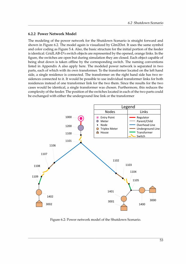
6.2 Shutdown Scenario

6.2.2 Power Network Model

The modeling of the power network for the Shutdown Scenario is straight forward andshown in Figure 6.2. The model again is visualized by Glm2Dot. It uses the same symboland color coding as Figure 5.4. Also, the basic structure for the initial portion of the feederis identical. GridLAB-D’s switch objects are represented by the opened, orange links. In thefigure, the switches are open but during simulation they are closed. Each object capable ofbeing shut down is taken offline by the corresponding switch. The naming conventionslisted in Appendix A also apply here. The modeled power network is separated in twoparts, each of which with its own transformer. To the transformer located on the left handside, a single residence is connected. The transformer on the right hand side has two re-sidences connected to it. It would be possible to use individual transformer links for bothresidences instead of one transformer link for the two them. Since the results for the twocases would be identical, a single transformer was chosen. Furthermore, this reduces thecomplexity of the feeder. The position of the switches located in each of the two parts couldbe exchanged with either the underground line link or the transformer

Nodes

Entry PointMeterNodeTriplex MeterHouse

RegulatorParent/ChildOverhead LineUnderground LineTransformerSwitch

LegendLinks

1000

1200

1100

1101

1102

1103

1104

1105

1400

3000

1401

3001

1106

1107

1108

1109

1402

3002

Figure 6.2: Power network model of the Shutdown Scenario.

53

6 Simulation & Results

6.2.3 Results

When looking at Figure 6.2, it becomes apparent, that different configurations for the Shut-down Scenario are possible. These configurations are summarized in Table 6.1. The figuredepicts all the possible configurations and their properties. The first configuration is cal-led the Initial configuration. Here, all components responsible for the power supply to theresidences are online and deliver a sufficient amount of energy. As a result, none of thethree houses is offline. The next configuration is Partial One, where the transformer withthe ID 1501 is taken offline by a falsified emergency shutdown request. Transformer 1500and the regulator, i.e., the substation, are still online and provide two out of the three resi-dences with energy. However, one of the residences, which is attached to Transformer 1501,is offline. In the Partial Two configuration, Transformer 1500 is taken offline, whereas theTransformer 1501 and the regulator remain online. Since two residences are attached tothis transformer, the total number of offline houses is two. In the last configuration, na-med Total, the regulator is taken offline. As a result, none of the transformers is suppliedwith power anymore. This means, that the three residences also receive no power and areoffline. The Total configuration is reached either by the regulator going offline as well asa subset of the two transformers or by both transformers going offline at the same time.Either way, the results are identical.

Configuration Regulator Transformer Transformer HousesName 1000 status 1500 status 1501 status offlineInitial online online online 0Partial One online online offline 1Partial Two online offline online 2Total offline offline offline 3

Tabelle 6.1: Configurations for the Shutdown Scenario.

The initial voltage values for the individual residences are given in Table 6.2. The similarityof the values is based simply on the flat structure of the simulated power network. Whena component of the electrical grid is going offline, the voltage measured at the meter of thehouse connected to the component drops from its initial value to 0V. This was the expectedoutcome.

House ID Initial Voltage3000 124.668V3001 124.615V3002 124.669V

Tabelle 6.2: Initial voltages for residences in the Shutdown Scenario.

The Shutdown Scenario provides the first proof of concept for CoPS, the implementationof the communication and power networks gives an easily accessible baseline model forfurther scenarios. To prevent the results of the Shutdown Scenario, precautions for mes-

54

6.3 Price Update Scenario

sage integrity and authenticity must be met. This could be, for example, comparison ofreceived messages with a reference message.

6.3 Price Update Scenario

In this section, the Price Update (PU) scenario is examined (see Chapter 4.2.2). The im-plementation for the partial models is covered in different sections. The communicationnetwork model is given in Section 6.3.1, the power network model in Section 6.3.2 respec-tively. The results of the simulated attack are discussed in Section 6.3.3.

6.3.1 Communication Network Model

For the PU scenario, the network structure shown in Figure 6.3 is conceived. The networkhas the same basic core structure as the SH model. However, since the PU scenario is mo-re complex than the SH scenario, the individual residences are grouped into streets andsubstreets due to the limitations of GridLAB-D’s data buffer (see Section 5.3). The streetsare the organizational units depicted in the GUI (see Chapter 5.4.3). The SubStreet com-ponent (symboled by a group of houses) is a compound module containing different resi-dences grouped together. It has been added to provide a better overview during modeling.All substreets suffixed with a certain identifier comprise the street, for example streetB1,streetB2, and streetB3 are referred to as Street B.

Figure 6.3: Communication network model of the Price Update Scenario.

55

6 Simulation & Results

6.3.2 Power Network Model

For the Price Update Scenario, a more complex power model is required. For this reason,an existing feeder model included is used. The feeder named R2-12.47-2, which is includedin the GridLAB-D distribution, is chosen because of its relative low count of nodes, whichis still large enough for a feasible presentation [48]. The feeder is operated with a voltageof 12.47 kV. A total of 189 residences are attached to the feeder.Figure 6.4 shows the structure of the R2-12.47-2 feeder. The symbols used are the same asin Figures 5.4 and 6.2. The newly introduced substreets are illustrated by gray boxes. As itcan be seen, the individual substreets of a given street N are a local cluster in the feeder.The grouping of the substreets as presented here took the arrangement of the residences inthe feeder into account. Houses close to each other are added to a cluster. Since the feederconsists of many nodes, a simplified illustration of the feeder’s structure is given at thispoint. A full representation of the feeder can be found in [14].

Nodes

Entry PointNodeSubstreet

Overhead LineUnderground LineSwitch

LegendLinks

A1

A2

A3

A4

A1

B3

B2

B1C3

C1 C2

C4

D1D2

D3

D5D4

D6

E1

E2

E5E3

E4

F1

F2

F3

G1

G3

G2

G4

Figure 6.4: Power network model of the Price Update Scenario.

56

6.3 Price Update Scenario

6.3.3 Results

Because of the complexity of the Price Update Scenario, the residences are arranged in lo-gical groups of streets and substreets. Table 6.3 summarizes the grouping process as alreadyshown in Figure 6.4. Only the streets will be of focus in the following since the substreetsdo not provide additional information. A street X is comprised of the substreets Xi withi ∈ N. Table 6.3 gives an overview of the seven streets to be found in the Price UpdateScenario. The number of residences per street varies from 15 to 45. This is due to the struc-ture of the distribution test feeder used in this scenario. The number of substreets is givenas well in the table. As mentioned in Section 5.3, randomly chosen residences are selectedas representative for a particular street. The meter reading from this residence will repre-sent the voltage of the entire street. The IDs of the selected residences are given in the lastcolumn. These representatives will be looked at in the following discussion of simulationresults. In the following, the terms street and representative are regarded as interchangeable.

Street Number of Number of ID of randomName residences substreets representativeA 15 4 10B 45 3 102C 31 4 121D 28 6 76E 28 5 23F 15 3 47G 27 4 187Total 189 29

Tabelle 6.3: Logical organization of residences and their properties for the Price UpdateScenario.

The results of the executed simulation for the Price Update Scenario are presented in Fi-gure 6.5. The voltage levels at the meter of each of the seven representatives is shownby a individual curve. The curve is labeled after their corresponding street. For example,Street A is the recorded value of Meter 10 and so on. For the simulation, the notificationshave all been sent at the same instance of time. The time these packets are received by theindividual components, however, differs. The simulation is run for 10 seconds, the messa-ges are sent at Second 1. After 3 seconds the streets A, B, and C receive the notifications andafter 5 seconds, the remaining streets have received the notifications as well. This two se-cond delays are due to a bottleneck, that occurred at router0 and router2 respectively(see Figure 6.3). Initially, all streets operate at the required voltage of above 120 V (dottedline). After the reception of the price update notifications, these values begin to fall by anaverage amount of 0.653V.

57

6 Simulation & Results

0 1 2 3 4 5 6 7 8 9 10119.8

120

120.2

120.4

120.6

120.8

121

121.2

121.4

121.6Voltage drop of selected residences after increase in demand

time [s]

voltage [V

]

Street AStreet BStreet CStreet DStreet EStreet FStreet G120VMessage

Figure 6.5: Measured voltage levels of representative residences of the streets A - G in thePrice Update Scenario.

58

6.3 Price Update Scenario

The voltage drop occurring in each street is summarized in Table 6.4. For some streets,the drop does not affect the required operating level but for Street B and Street C the vol-tage value drops below 120 V. For Street B, the voltage dropped from the initial value of120.603V to 119.988V (a difference of 0.615V). For Street C, the drop was from 120.573V to119.878V (0.695V difference). In a real world scenario, the result could be brownouts in theresidences located in those streets. A larger voltage drop caused by an increased numberof appliances, that are connected to the grid at the same time, was expected. With 189 si-mulated residences, the occurring voltage drop was for most of them without any furtherconsequences. Some of the residences would suffer from dimmed lights and similar nui-sances but drastic effects on the residences or the distribution network are not discovered.

Street Initial Voltage after DifferenceName voltage received messageA 120.715 120.380 0.335B 120.603 119.988 0.615C 120.573 119.878 0.965D 121.306 120.662 0.644E 121.392 120.594 0.798F 121.405 120.598 0.807G 121.199 120.521 0.678Average 121.038 120.374 0.653

Tabelle 6.4: Voltage drops occurring in streets of the Price Update Scenario after receivingprice update notifications.

59

7 Conclusion & Future Work

In this chapter, the results of the thesis are summarized. In Section 7.1, conclusions arepresented. Section 7.2 outlines possibilities for future work and addresses open problems.

7.1 Conclusion

In this thesis, a framework for conducting security analyses in future Smart Grids is deve-loped, the Communication & Power Network Co-Simulation (CoPS). With CoPS, attackson Smart Grids originating from the integrated communication network are defined, exe-cuted, and their results are examined. Since Smart Grids will play an important role in thefuture of the energy sector, this could draw interest from power companies. In addition,private consumers and prosumers are going to be integrated into the Smart Grid via smartmeter and gateways, that are also a potential target for attackers. Manipulated messagespropagated though the network infrastructure could have far-reaching consequences onthe security of supply. To study the results of such attacks and to create a sense of awa-reness among stakeholders, modeling and simulation is the tool of choice. A concept forthe integration of the required simulators is developed and implemented. The frameworkcombines for the first time the simulators OMNeT++ and GridLAB-D together to a co-simulation. It is the first Smart Grid security simulation framework composed from opensource frameworks. Moreover, for the first time both domains customer and energy distri-bution are taken into account for security studies on Smart Grids. Two attack vectors areconceptualized, implemented, and simulated using the framework. The generated data isanalyzed and used to estimate the potential consequences of the simulated attack vectors.The Shutdown Scenario is the first scenario and acts as the proof of concept for CoPS. Itfurther demonstrates the effects a forcible removed component can have on the electricalgrid and the security of supply. The Price Update Scenario gives an first insight in thefull capabilities of CoPS. Inside a complex and realistic distribution network, a total of 189residences with smart meter and gateways are simulated. The gateways all receive ma-nipulated price update notifications and according to the new price, the demand of therespective residence is changed to meet the new market conditions, i.e., household app-liances are turned on or off. The findings of the simulation run shows, that this scenarioleads to a voltage drop, which might cause the voltage to go down below the thresholdfor the required voltage of 120V. However, the magnitude of the drops is with an averagedifference of 0.653 V not as high as expected. The simulated scenario with 189 residenceswas, however, a small scale scenario. In a bigger network with more consumers the effectsof such an attack would be more extensive. Furthermore, the water heater objects usedas appliances are not characterized by high demand as opposed to, for example, electriccars. The study of a large scale scenario with different types of consumers, as outlinedin the subsequent section, might provide interesting results. In general, the results of the

61

7 Conclusion & Future Work

simulations show, that securing of packet traffic between the components is necessary tocounteract the effects of the described attack vectors. The integrity and authenticity of thetransmitted control commands must be guaranteed. The further use of unprotected SCA-DA networks connected via public networks is not advisable.

7.2 Future Work

The Price Update Scenario shows, that an effect of manipulated price update messages ispresent. In the simulated power network, this has only a low impact on the security of sup-ply. This will probably be different in other scenarios, where not only private consumersare present. The energy consumption by sector in Germany in 2011 is given in Figure 7.1.The energy consumption of private consumers is 27% but the combined energy consump-tion of the industry and commerce sector is as high as 70% [19]. This raises the question,if the study of an attack vector, which targets private households, needs to be conductedwith the effort it has been previously. For this reason, including industry and commercemight be a reasonable consideration for further research. For this, the Commercial modu-le of GridLAB-D could be used, when it has been extended further. At the moment, onlymodels for small office buildings are included but an extension of the module in futureversions is planned. In combination with the Generators module, the simulation couldfurther be extended to include, for example, wind mills.

27%

42%

28%

3%

Diagrammtitel

Households Industry Commerce Transport

Figure 7.1: Energy consumption by sector in Germany in 2011 (Source: [19]).

7.2.1 Power Network Model

GridLAB-D also offers its own wholesale market module providing integration of pricingmodels for energy into the simulation. Integrating the market domain into the simulationincreases the detail of the simulation further. Also, this a step towards a simulation frame-work encompassing all aspects of the Smart Grid. The market module could be replacedwith AMES, a wholesale power market test bed developed for research purposes. AMESoffers a more detailed model of the market and has already been employed successfully

62

7.2 Future Work

with GridLAB-D in a co-simulation with a concept similar to that of CoPS [10]. In addition,using pricing models also offers the possibilities of providing an estimate for the damagecaused by an attack. The Integrated Retail and Wholesale (IRW) project uses a synchronousexecution mode. The co-simulation of IRW employs GridLAB-D and AMES, an in-housedevelopment, to conduct market research on price developments in Smart Grids. A spe-cialized data management program and a MySQL server are used for message exchangeand synchronization.In addition of employing previously unused GridLAB-D modules, the already used mo-dules could be extended. In particular, the Powerflow module is well-suited for this. Thecomponents of the Powerflow module provide currently no possibility for reading outfrequency values measured in Hertz. These values, however, are an important indicatorfor the stability of the power network [53]. Being able to tap into the frequency and provi-de proper readings of it, provides new ways of examining the effects of an attack. The sta-bility of the energy supply could be examined more closely. Additionally, the Powerflowmodule could be enhancement by improving the underground and overground line mo-dels. Simulating the overload of a line is currently also not possible. However, this additionmight prove challenging since it will probably require modification to the solver methodsbecause the underground and overground links are an essential part for the computationof the power demand.The electrical components modeled in CoPS are based on the conditions of the power net-work in the USA. This is due to nature of GridLAB-D’s funding by the U.S. Department ofEnergy. For future investigation, however, models reflecting the conditions in Germany aremore reasonable. This includes the adjustment of voltage levels found at low and middlevoltage areas. Also, a feeder model derived from base data of German feeder models ismeaningful. Another part for localization is the data for the weather model. The weatherdoes not have any influence on the power network models in CoPS so far since no solarcollectors or wind mills have been employed into the simulated scenarios. Models for tho-se components, however, are present in CoPS and could be used in future simulations. Theweather data needs to be in the Typical Meteorological Year (TMY) format [48].

7.2.2 Communication Network Model

The scheduler for OMNeT++ used by CoPS is capable of real-time simulation. For this re-ason, hardware-in-the-loop simulations are possible since the clock of an external devicecould be synchronized with the internal clock of the simulation. This offers the possibilityof including real life components, for example smart meter and gateways, into the simula-tion. This could lead to an entire test bed for those components.The packet-based communication in OMNeT++ is an area where enhancements could pro-vide a better simulation model. At this point, packet-based communication only occurs inthe simulation as a result of an user action. This is not very realistic since a model for the In-ternet is included in the communication network. It is more likely, that other components,for example a private PC located at the customer, utilize this network as well. Therefore,models adding traffic to the network could be included in CoPS. This could be done, forexample, with OMNeT++’s InternetBrowser component [4].The traffic between the gateway and the smart meter is modeled at an abstract level, mea-ning no protocols are employed on this data channel. SCADA systems use their own family

63

7 Conclusion & Future Work

of protocols [17]. A large number of these protocols exists, which makes the implementati-on of each SCADA protocol a time consuming task. Implementation of a small number ofselected protocols is much more feasible. Existing implementations of Modbus and DNP3for older versions of OMNeT++ exist and could be ported to CoPS [44]. Other protocolsworth considering due to their prevalence are PROFIBUS and IEC 60870.5.During simulation it has been found, that the Price Update Scenario takes a long time toload all of the 189 modeled houses in OMNeT++. In [40], the authors present a scalable so-lution encompassing OMNeT++, that is capable of simulating 10.000 houses. The modeledlarge scale scenario is related to Smart Grid but does not contain a model for the powernetwork so far. As mentioned in the beginning of Section 7.2, a large scale model mightprovide different results then the model used in the Price Update Scenario.

64

Appendix

65

Appendix A Naming Conventions forGridLAB-D

Listed below is the naming convention used to identify objects in large GridLAB-D models.The numbers represent the IDs assigned to each object inside the model. Each relevantmodule (see Chapter 2.2.3) is assigned a four digit namespace. The configuration objectsof the Powerflow module are assigned to an individual namespace due to their quantity.The objects found in this namespace are then grouped accordingly. For example, the firstnode of a model has the ID 1100 assigned to, the second node 1101 and so on.

• 1xxx Powerflow ModuleComponents of the distribution network.

– 10xx Regulators

– 11xx Nodes

– 12xx Meter

– 13xx Triplex Nodes

– 14xx Triplex Meter

– 15xx Transformers

– 16xx Overground Lines

– 17xx Underground Lines

– 18xx Triplex Lines

– 19xx Switches

• 2xxx Powerflow Module ConfigurationsConfiguration objects for the distribution network components.

– 20xx Regulator Configuration

– 21xx Line Configuration

– 22xx Line Spacing

– 23xx Triplex Line Configuration

– 25xx Transformer Configuration

– 26xx Overhead Line Conductor

– 27xx Underground Line Conductor

– 28xx Triplex Line Conductor

67

A Naming Conventions for GridLAB-D

• 3xxx Residential ModuleHouses and their appliances.

– 30xx Houses

– 31xx - 32xx Enduses, i.e. household appliances

* 310x Clotheswasher

* 311x Dishwasher

* 312x Dryer

* 313x Evcharger

* 314x Freezer

* 315x Lights

* 316x Microwave

* 317x Occupantload

* 318x Plugload

* 319x Range

* 320x Refrigerator

• 4xxx Generators ModuleEnergy generation from renewable sources and energy storage components. Thismodule is developed mostly by the community.

– 40xx Wind Mills

– 41xx Solar Collectors

– 42xx Inverter

– 43xx Battery

– 44xx Diesel Generator

– 45xx Microturbine

• 5xxx Reliability ModuleObjects for reliability analysis. In the thesis used for opening and closing switches.

– 50xx Fault Check

– 51xx Metrics

– 52xx Eventgen

– 53xx Power Metrics

• 6xxx Tape ModuleRecorder for reading measurements inside the simulation and for exporting the mea-sured values.

– 60xx Recorders

– 61xx Multi Recorders

68

Appendix B How to use the Framework

This chapter outlines how CoPS is supposed to be used. First, the installation procedure isexplained in Section B.1. Then, Section B.2 explains how the included demo simulations ofthe framework can be executed and run. A tutorial for adding new simulations to CoPS ispresented in the subsequent Section B.3.

B.1 Installation of CoPS

CoPS has been developed on Windows 7 x64 with the latest patches as of May 2013. Formodeling communication networks, OMNeT++ 4.2.2 and INET 2.1 were used. CoPS willprobably work with newer versions of both software packages, however, this has not beentested. The installation of OMNeT++ and INET follows the instructions included in therespective package. A bug in the linker of MinGW for Windows 7 x64 might cause INETnot to be built properly. The issue is resolved by reinstalling both, OMNeT++ and INET.The power network models use GridLAB-D 2.2. Newer versions of GridLAB-D might notbe compatible. Further, the .NET 4.5 framework is required, as well as Visual Studio 2012.To use the network capability of CoPS, modifications to the hosts file are necessary. Thefollowing entry has to be added to the hosts file:

127.0.0.1 localhost cops.aisec

Listing B.1: Required entry into the hosts file of Windows.

B.2 Running the included simulations

Two demo applications, the Shutdown Scenario and the Price Update Scenario (see Chap-ter 5.2 and Chapter 5.3) respectively, are included in CoPS. The following steps are neces-sary for using any of these demos:

1. Start OMNeT++ and run the respective simulation of the communication network.This is achieved by right-clicking the omnetpp.ini file in the model’s folder and se-lecting Run As OMNeT++ Simulation. After the model is loaded, start the simulationof the communication network by pressing Run. The components with sockets thenimmediately start listening for incoming packets.

2. Run the .NET server application and start the server. The address of the server ispreset to http://cops.aisec:8080/.

3. Run the main GUI of CoPS (see Figure 5.8).

69

B How to use the Framework

a) Select the respective simulation.

b) Load the corresponding model of the power network.

c) The Winsock server is preset to http://localhost:4242 and does not needto be changed.

d) Do simulation specific tasks by navigating to the corresponding tab on the GUI.In the Shutdown Scenario, components are taken offline by selecting them. Inthe Price Update Scenario, prices are changed and sent. If the prices have de-cimal places, use the American format for separating them, i.e., a dot (“.”) isrequired instead of a comma (“,”).

e) When finished, i.e., the last task has been conducted, press the finalize button tosimulate the last step and to finish the simulation.

4. The results computed by GridLAB-D during each simulation step are not deleted.They are, instead, stored in the same folder where the power network model file islocated (see Step 3b).

The execution order for steps 1 and 2 of the above enumeration is interchangeable.

B.3 Adding new simulations

The architecture of CoPS is designed to allow adding own simulations. Each scenario re-quires a model for communication network and for the power network. The implementa-tions of the demo scenarios, Price Update and Shutdown, can be taken as guidelines (seeChapter 5.2 and Chapter 5.3). It is recommended to enforce the naming conventions listedin Appendix A.The simulations further need to be integrated in .NET. This is done by adding a new simu-lation class, which is subclassed from the abstract Simulation class (see Chapter 5.4.2).Most of the existing implementation for the included scenarios can be adopted for the newclasses. Only the simulation specific tasks might require some additional work.The user interface needs to be updated as well. This is done by adding a new tab to theTabControl, where the user is able to perform simulation specific actions. These acti-ons need to implemented in the aforementioned new simulation class. If new componentsare used inside the power network model, images for displaying these components in thePowerStructure user control need to be provided. The images used by the included si-mulations have the size 48x48 and are Portable Network Graphics (PNG). However, othersizes and file types may be used as well. The new images must be added to the imagesfolder inside of Visual Studio. Their Build Action property needs to be set to Embedded Re-source. They further must be loaded inside the constructor of the PowerStructure usercontrol in order to be used by the control. The existing implementation provides the detailsfor this task.

70

List of Figures

1.1 Estimated change in the energy mix of Germany until 2030 (Source: [19]). . 21.2 Conceptual structure of a Smart Grid (Source: [17]). . . . . . . . . . . . . . . 3

2.1 Conceptual view of SCADA system architecture. . . . . . . . . . . . . . . . . 82.2 Simplified domains and connections among them (Source (updated): [18]). . 92.3 Structural view of ns2’s main components. . . . . . . . . . . . . . . . . . . . 122.4 OMNeT++’s NED Editor showing a simple UDP-based network. . . . . . . 13

4.1 Categorization of existing co-simulation frameworks. . . . . . . . . . . . . . 214.2 HLA federation. . . . . . . . . . . . . . . . . . . . . . . . . . . . . . . . . . . . 224.3 Time-stepped simulation run. . . . . . . . . . . . . . . . . . . . . . . . . . . . 244.4 Asynchronous execution of a time-stepped simulation run. . . . . . . . . . . 264.5 Conceptual view of the Shutdown attack. . . . . . . . . . . . . . . . . . . . . 304.6 Conceptual view of the Price Update attack. . . . . . . . . . . . . . . . . . . . 32

5.1 Components and packages of the communication and power network co-simulation. . . . . . . . . . . . . . . . . . . . . . . . . . . . . . . . . . . . . . . 34

5.2 Gateway component of CoPS during runtime of a Price Update attack. . . . 365.3 Subnetworks implemented in CoPS. . . . . . . . . . . . . . . . . . . . . . . . 375.4 Visualization of a simple GridLAB-D distribution feeder. . . . . . . . . . . . 385.5 Classes for implementation of the Strategy Pattern in CoPS. . . . . . . . . . 435.6 Asynchronous execution of the co-simulation with CoPS. . . . . . . . . . . . 445.7 Algorithm for advancing the simulation. . . . . . . . . . . . . . . . . . . . . . 465.8 Main GUI of CoPS during a Shutdown simulation. . . . . . . . . . . . . . . . 475.9 Actions and states of CoPS’s main GUI. . . . . . . . . . . . . . . . . . . . . . 485.10 Visualized power network structure for the Price Update Scenario. . . . . . 49

6.1 Communication network model of the Shutdown Scenario. . . . . . . . . . . 526.2 Power network model of the Shutdown Scenario. . . . . . . . . . . . . . . . 536.3 Communication network model of the Price Update Scenario. . . . . . . . . 556.4 Power network model of the Price Update Scenario. . . . . . . . . . . . . . . 566.5 Measured voltage levels of representative residences of the streets A - G in

the Price Update Scenario. . . . . . . . . . . . . . . . . . . . . . . . . . . . . . 58

7.1 Energy consumption by sector in Germany in 2011 (Source: [19]). . . . . . . 62

71

References

[1] IEEE Guide for Electric Power Distribution Reliability Indices. IEEE Std 1366-2003,pages 1–50, 2003.

[2] IEEE Standard for Modeling and Simulation (M & S) High Level Architecture (HLA)–Framework and Rules. IEEE Std 1516-2010 (Revision of IEEE Std 1516-2000), pages 1–38, 2010.

[3] INET framework 2.0 for OMNeT++. Manual., 2011.

[4] INET framework 2.1 for OMNeT++. Manual., 2012.

[5] Programmable controllers - Part 3: Programming languages. IEC 61131-3 ed 3.0, pages1–464, 2013.

[6] International Energy Agency. World Energy Outlook, 2012. OECD/IEA, 2012.

[7] Thomas Andrew. Developing SCADA Simulations with C2WindTunnel. 2011.

[8] Martin Brunner, Hans Hofinger, Christoph Krauß, Christopher Roblee, P. Schoo, andS. Todt. Infiltrating critical infrastructures with next-generation attacks. FraunhoferInstitute for Secure Information Technology (SIT), Munich, 2010.

[9] H.J. Bungartz, S. Zimmer, M. Buchholz, and D. Pflüger. Modellbildung und Simulation:Eine Anwendungsorientierte Einführung. Springer London, Limited, 2009.

[10] Chengrui Cai, Pedram Jahangiri, Auswin George Thomas, Huan Zhao, Dionysios C.Aliprantis, and Leigh Tesfatsion. Agent-based simulation of distribution systems withhigh penetration of photovoltaic generation. In Power and Energy Society General Mee-ting, 2011 IEEE, pages 1–7. IEEE, 2011.

[11] Rohan Chabukswar, Bruno Sinópoli, Gabor Karsai, Annarita Giani, Himanshu Nee-ma, and Andrew Davis. Simulation of network attacks on SCADA systems. In Pro-ceedings of the First Secure Control Systems Workshop, Cyberphysical Systems Week, Stock-holm, Sweden, 2010.

[12] D.P. Chassin, K. Schneider, and C. Gerkensmeyer. GridLAB-D: An open-source powersystems modeling and simulation environment. In Transmission and Distribution Con-ference and Exposition, 2008. T&D. IEEE/PES, pages 1–5. IEEE, 2008.

[13] Claudia Eckert and Christoph Krauß. Sicherheit im Smart Grid - Herausforderungenund Handlungsempfehlungen. Datenschutz und Datensicherheit, 8:535–541, 2011.

73

References

[14] Michael A. Cohen. GridLAB-D Taxonomy Feeder Graphs. http://emac.berkeley.edu/gridlabd/taxonomy_graphs/. Accessed on March 4,2013.

[15] Wireless Communication and Information Processing Lab. Comparative view of OM-Net++ and ns-2. http://www.wicip.ca/index.php/wicip-resources/82-wicip-main/wicip-resource-articles/74-wicip-ns2-or-omnetpp. Ac-cessed on January 11, 2013.

[16] C. Eckert. IT-Sicherheit: Konzepte, Verfahren, Protokolle. Oldenbourg, 2008.

[17] Claudia Eckert and Christoph Krauß. Sicherheit im Smart Grid. Datenschutz undDatensicherheit-DuD, 35(8):535–541, 2011.

[18] Claudia Eckert and Christoph Krauß. Sicherheit im Smart Grid - Sicherheitsarchi-tekturen für die Domänen Privatkunde und Verteilnetz unter Berücksichtigung derElektromobilität. Alcatel-Lucent Stiftung, Stiftungsreihe 96, 2012.

[19] Arbeitsgemeinschaft Energiebilanzen eV. Auswertungstabellen zur Energiebilanz fürdie Bundesrepublik Deutschland 1990 bis 2011, 2012.

[20] Miguel A. Erazo, Ting Li, Jason Liu, and Stephan Eidenbenz. Toward comprehensiveand accurate simulation performance prediction of parallel file systems. In DependableSystems and Networks (DSN), 2012 42nd Annual IEEE/IFIP International Conference on,pages 1–12. IEEE, 2012.

[21] J.C. Fuller and K.P. Schneider. Modeling Wind Turbines in the GridLAB-D SoftwareEnvironment. Journal of Undergraduate Research, 9, 2009.

[22] E. Gamma, R. Helm, R. Johnson, and J. Vlissides. Design Patterns: Elements of ReusableObject-Oriented Software. Pearson Education, 1994.

[23] Tim Godfrey, Sara Mullen, Roger C. Dugan, Craig Rodine, David W. Griffith, andNada Golmie. Modeling smart grid applications with co-simulation. In Smart GridCommunications (SmartGridComm), 2010 First IEEE International Conference on, pages291–296. IEEE, 2010.

[24] Ian Griffiths. Programming C# 5.0: Building Windows 8, Web, and Desktop Applicationsfor the. NET 4.5 Framework. O’Reilly Media, Incorporated, 2012.

[25] Thomas R. Henderson, Mathieu Lacage, George F. Riley, C. Dowell, and J.B. Kopena.Network simulations with the ns-3 simulator. SIGCOMM demonstration, 2008.

[26] Kenneth Hopkinson, Xiaoru Wang, Renan Giovanini, James Thorp, Kenneth Birman,and Denis Coury. EPOCHS: A platform for agent-based electric power and commu-nication simulation built from commercial off-the-shelf components. Power Systems,IEEE Transactions on, 21(2):548–558, 2006.

[27] K.M. Hopkinson, K.P. Birman, R. Giovanini, D.V. Coury, X. Wang, and J.S. Thorp.EPOCHS: Integrated commercial off-the-shelf software for agent-based electric power

74

References

and communication simulation. In Simulation Conference, 2003. Proceedings of the 2003Winter, volume 2, pages 1158–1166 vol.2, 2003.

[28] Vinay M. Igure, Sean A. Laughter, and Ronald D. Williams. Security issues in SCADAnetworks. Computers & Security, 25(7):498–506, 2006.

[29] Battelle Memorial Institute. GridLAB-D Repository. http://sourceforge.net/projects/gridlab-d/. Accessed on February 13, 2013.

[30] U.C. Irvine, J. Gettys, J. Mogul, H. Frystyk, L. Masinter, P. Leach, and T. Berners-Lee.Hypertext Transfer Protocol – HTTP/1.1. RFC 2616, 1999.

[31] Pedram Jahangiri, Di Wu, Wanning Li, Dionysios C. Aliprantis, and Leigh Tesfatsion.Development of an agent-based distribution test feeder with smart-grid functionality.In Power and Energy Society General Meeting, 2012 IEEE, pages 1–7. IEEE, 2012.

[32] W.H. Kersting. Radial distribution test feeders. In Power Engineering Society WinterMeeting, 2001. IEEE, volume 2, pages 908–912. IEEE, 2001.

[33] Michael Lesk. The new front line: Estonia under cyberassault. Security & Privacy,IEEE, 5(4):76–79, 2007.

[34] Martin Lévesque, Da Qian Xu, Géza Joós, and Martin Maier. Communications andpower distribution network co-simulation for multidisciplinary smart grid experi-mentations. In Proceedings of the 45th Annual Simulation Symposium, page 2. Society forComputer Simulation International, 2012.

[35] W. Li, A. Monti, M. Luo, and Roger A. Dougal. VPNET: A co-simulation frameworkfor analyzing communication channel effects on power systems. In Electric Ship Tech-nologies Symposium (ESTS), 2011 IEEE, pages 143–149. IEEE, 2011.

[36] Hua Lin. Communication Infrastructure for the Smart Grid: A Co-Simulation Based Stu-dy on Techniques to Improve the Power Transmission System Functions with Efficient DataNetworks. PhD thesis, Virginia Polytechnic Institute and State University, 2012.

[37] Hua Lin, Santhosh S. Veda, Sandeep S. Shukla, Lamine Mili, and James Thorp. GE-CO: Global Event-Driven Co-Simulation Framework for Interconnected Power Sy-stem and Communication Network. Smart Grid, IEEE Transactions on, 3(3):1444–1456,2012.

[38] Christoph P. Mayer and Thomas Gamer. Integrating real world applications into OM-NeT++. Institute of Telematics, University of Karlsruhe, Karlsruhe, Germany, Tech. Rep.TM-2008-2, 2008.

[39] Steven McCanne, Sally Floyd, Kevin Fall, Kannan Varadhan, et al. Network simulatorns-2, 1997.

[40] Christian Müller, Hanno Georg, and Christian Wietfeld. A modularized and distribu-ted simulation environment for scalability analysis of smart grid ICT infrastructures.

75

References

In Proceedings of the 5th International ICST Conference on Simulation Tools and Techni-ques, pages 327–330. ICST (Institute for Computer Sciences, Social-Informatics andTelecommunications Engineering), 2012.

[41] B. Müller-Rathgeber and Holm Rauchfuss. A cosimulation framework for a distribu-ted system of systems. In Vehicular Technology Conference, 2008. VTC 2008-Fall. IEEE68th, pages 1–5. IEEE, 2008.

[42] Nitsch, Joachim and Pregger, Thomas and Scholz, Yvonne and Sterner, Michael andGerhardt, Norman and von Oehsen, Amany and Pape, Carsten and Saint-Drenan,Yves-Marie and Wenzel, Bernd. Langfristszenarien und Strategien für den Ausbauder erneuerbaren Energien in Deutschland bei Berücksichtigung der Entwicklung inEuropa und global. Entwurf Zwischenbericht. Mai, 2010.

[43] James Nutaro, Phani Teja Kuruganti, Laurie Miller, Sara Mullen, and MallikarjunShankar. Integrated hybrid-simulation of electric power and communications sy-stems. In Power Engineering Society General Meeting, 2007. IEEE, pages 1–8. IEEE, 2007.

[44] Carlos Queiroz, Abdun Mahmood, and Zahir Tari. SCADASim - A framework forbuilding SCADA simulations. Smart Grid, IEEE Transactions on, 2(4):589–597, 2011.

[45] Derek Riley, Emeka Eyisi, Jia Bai, Xenofon Koutsoukos, Yuan Xue, and Janos Szti-panovits. Networked control system wind tunnel (NCSWT): an evaluation tool fornetworked multi-agent systems. In Proceedings of the 4th International ICST Conferenceon Simulation Tools and Techniques, pages 9–18. ICST (Institute for Computer Sciences,Social-Informatics and Telecommunications Engineering), 2011.

[46] James A. Rowson. Hardware/software co-simulation. In Design Automation, 1994.31st Conference on, pages 439–440. IEEE, 1994.

[47] Victorino Sanz. Hybrid System Modeling: Using the Parallel DEVS Formalism andthe Modelica Language. 2011.

[48] Kevin P. Schneider, Yousu Chen, David P. Chassin, Robert G. Pratt, David W. Engel,and Sandra Thompson. Modern grid initiative: Distribution taxonomy final report. PacificNorthwest National Laboratory, 2008.

[49] Kevin P. Schneider, Yousu Chen, D. Engle, and D. Chassin. A taxonomy of NorthAmerican radial distribution feeders. In Power & Energy Society General Meeting, 2009.PES’09. IEEE, pages 1–6. IEEE, 2009.

[50] SZ Online. Blackout legt München lahm. Süddeutsche Zeitung. http://sz.de/1.1523769. Accessed on December 12, 2012.

[51] András Varga and Rudolf Hornig. An overview of the OMNeT++ simulation envi-ronment. In Proceedings of the 1st international conference on Simulation tools and techni-ques for communications, networks and systems & workshops, page 60. ICST (Institute forComputer Sciences, Social-Informatics and Telecommunications Engineering), 2008.

[52] András Varga. OMNeT++ User Manual Version 4.2.2. OpenSim Ltd., 2011.

76

References

[53] Von Meier, Alexandra. Electric power systems: a conceptual introduction. Wiley-Interscience, 2006.

[54] Elias Weingartner, Hendrik Vom Lehn, and Klaus Wehrle. A performance compari-son of recent network simulators. In Communications, 2009. ICC’09. IEEE InternationalConference on, pages 1–5. IEEE, 2009.

[55] Zhi Zhang, Zhonghai Lu, Qiang Chen, Xiaolang Yan, and Li-Rong Zheng. COSMO:CO-simulation with MATLAB and OMNeT++ for indoor wireless networks. In GlobalTelecommunications Conference (GLOBECOM 2010), 2010 IEEE, pages 1–6. IEEE, 2010.

77