Full-wave method of calculation of electromagnetic fields ...nlpc.stanford.edu/nleht/Science/talks/2011/ICEAA_Lehtinen_FWM_talk.pdf · Full-wave method of calculation of electromagnetic

STANFORDE L E C T R I C A LE N G I N E E R I N G

Full-wave method of calculation of electromagneticfields in stratified media

Nikolai G. Lehtinen, Timothy F. Bell, Umran S. Inan

STAR Laboratory, Stanford University, Stanford, CA, U.S.A.ICEAA ’11, Torino, Italy

September 15, 2011

STANFORDE L E C T R I C A LE N G I N E E R I N G

N. Lehtinen (Stanford) Full-wave method September 15, 2011 1

Stanford Full-Wave Method (SFWM) code STANFORDE L E C T R I C A LE N G I N E E R I N G

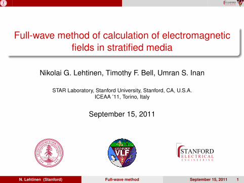
Outline

1 Stanford Full-Wave Method (SFWM) codeCapabilitiesDescription

2 Applications of SFWMWave propagation through ionosphereModulated electrojet VLF radiationVLF transmitter radiationRadiation from lightningEarth-ionosphere waveguide modesScattering on ionospheric disturbances

3 Conclusions

4 Extra slides


Stanford Full-Wave Method (SFWM) code Capabilities STANFORDE L E C T R I C A LE N G I N E E R I N G

Outline



3 Conclusions

4 Extra slides


Stanford Full-Wave Method (SFWM) code Capabilities STANFORDE L E C T R I C A LE N G I N E E R I N G

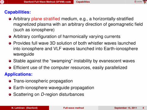
Capabilities:Arbitrary plane stratified medium, e.g., a horizontally-stratifiedmagnetized plasma with an arbitrary direction of geomagnetic field(such as ionosphere)Arbitrary configuration of harmonically varying currentsProvides full wave 3D solution of both whistler waves launchedinto ionosphere and VLF waves launched into Earth-ionospherewaveguideStable against the “swamping” instability by evanescent wavesEfficient use of the computer resources, easily parallelized

Applications:Trans-ionospheric propagationEarth-ionosphere waveguide propagationScattering on D-region disturbances


Stanford Full-Wave Method (SFWM) code Description STANFORDE L E C T R I C A LE N G I N E E R I N G

Outline



3 Conclusions

4 Extra slides



z

xy

Ne

B

z2

zk

zk+1

zM

z1=0

εk

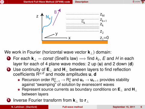
We work in Fourier (horizontal wave vector k⊥) domain:1 For each k⊥ = const (Snell’s law) =⇒ find kz , E and H in each

layer for each of 4 plane wave modes: 2 up (u) and 2 down (d)2 Use continuity of E⊥ and H⊥ between layers to find reflection

coefficients Ru,d and mode amplitudes u, dRecursion order Ru

k+1 → Ruk and uk → uk+1 provides stability

against “swamping” of solution by evanescent wavesRepresent source currents as boundary conditions on E⊥ and H⊥between layers

3 Inverse Fourier transform from k⊥ to r⊥N. Lehtinen (Stanford) Full-wave method September 15, 2011 6


Full-wave method backgroundGeneral description of waves in stratified media and reviews:

Altman, C., and K. Suchy (1991), Reciprocity, Spatial Mapping and Time Reversal in Electromagnetics, Kluwer AcademicPublishers, Boston.

REVIEW: Budden, K. G. (1985), The Propagation of Radio Waves: The Theory of Radio Waves of Low Power in theIonosphere and Magnetosphere, Cambridge Univ. Press, Cambridge, Chapter 18.

Clemmow, P. C., and J. Heading (1954), Coupled forms of the differential equations governing radio propagation in theionosphere, Math. Proc. of the Cambridge Phil. Soc., 50(2), 319–333, doi:10.1017/S030500410002939X.

Wait, J. R. (1970), Electromagnetic Waves in Stratified Media, 2nd ed., Pergamon, New York.Methods using subtraction of growing evanescent mode proposed by Pitteway [1965], The numerical calculation of wave-fields,reflexion coefficients and polarizations for long radio waves in the lower ionosphere I, Phil. Trans. R. Soc. London, Ser. A,257(1079), 219–241:

Nagano, I., K. Miyamura, S. Yagitani, I. Kimura, T. Okada, K. Hashimoto, and A. Y. Wong (1994), Full wave calculationmethod of VLF wave radiated from a dipole antenna in the ionosphere — analysis of joint experiment by HIPAS andAkebono satellite, Electr. Commun. Jpn. Commun., 77(11), 59–71, doi:10.1002/ecja.4410771106.

Scarabucci, R. R. (1969), Analytical and numerical treatment of wave-propagation in the lower ionosphere, Tech. ReportNo. 3412-11, Stanford University, Stanford, CA.

Yagitani, S., I. Nagano, K. Miyamura, and I. Kimura (1994), Full wave calculation of ELF/VLF propagation from a dipolesource located in the lower ionosphere, Radio Sci., 29(1), 39–54, doi:10.1029/93RS01728.

Methods using the same recursion order as the one described here:

Nygren, T. (1982), A method of full wave analysis with improved stability, Planet. Space Sci., 30(4), 427–430,doi:10.1016/0032-0633(82)90048-4.

Wang, T.-I. (1971), Intermode coupling at ion whistler frequencies in a stratified collisionless ionosphere, J. Geophys.Res., 76(4), 947–959, doi:10.1029/JA076i004p00947.

Other methods:Using “matrizants”, e.g.: Bossy, L. (1979), Wave propagation in stratified anisotropic media, J. Geophys., 46, 1–14.


Applications of SFWM STANFORDE L E C T R I C A LE N G I N E E R I N G

Outline



3 Conclusions

4 Extra slides


Applications of SFWM Wave propagation through ionosphere STANFORDE L E C T R I C A LE N G I N E E R I N G

Outline



3 Conclusions

4 Extra slides



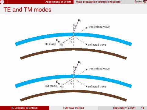
TE and TM modes

θi

θB

B0

H

ETE mode

transmitted wave

reflected wave

θi

θB

B0

E

HTM mode

transmitted wave

reflected wave



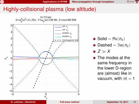
Highly-collisional plasma (low altitude)

−5 0 5−5

−4

−3

−2

−1

0

1

2

3

4

5

nx

n y

h=73 kmX=ω

p2/ω2=11.201, Y=ω

H/ω=139.96, Z=ν/ω=68.509

UP: n

1

UP: n2

DOWN: n3

DOWN: n4

Geomagnetic field Solid = Re(nz)

Dashed = Im(nz)

Z � XThe modes at thesame frequency inthe lower D-regionare (almost) like invacuum, with |n| = 1



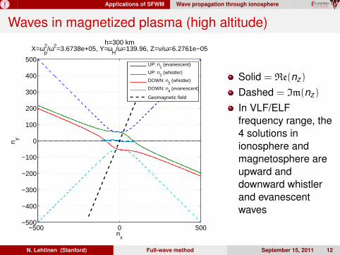
Waves in magnetized plasma (high altitude)

−500 0 500−500

−400

−300

−200

−100

0

100

200

300

400

500

nx

n y

h=300 kmX=ω

p2/ω2=3.6738e+05, Y=ω

H/ω=139.96, Z=ν/ω=6.2761e−05

UP: n

1 (evanescent)

UP: n2 (whistler)

DOWN: n3 (whistler)

DOWN: n4 (evanescent)

Geomagnetic field

Solid = Re(nz)

Dashed = Im(nz)

In VLF/ELFfrequency range, the4 solutions inionosphere andmagnetosphere areupward anddownward whistlerand evanescentwaves



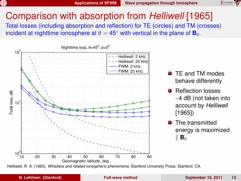
Comparison with absorption from Helliwell [1965]Total losses (including absorption and reflection) for TE (circles) and TM (crosses)incident at nighttime ionosphere at θ = 45◦ with vertical in the plane of B0.

10 20 30 40 50 60 70 80 9010

0

101

102

Geomagnetic latitude, deg

Tota

l lo

ss, dB

Nighttime loss, θ=45o; φ=0

o

Helliwell: 2 kHz

Helliwell: 20 kHz

FWM: 2 kHz

FWM: 20 kHz TE and TM modesbehave differently

Reflection losses∼4 dB (not taken intoaccount by Helliwell[1965])

The transmittedenergy is maximized‖ B0

Helliwell, R. A. (1965), Whistlers and related ionospheric phenomena, Stanford University Press, Stanford, CA.


Applications of SFWM Modulated electrojet VLF radiation STANFORDE L E C T R I C A LE N G I N E E R I N G

Outline



3 Conclusions

4 Extra slides



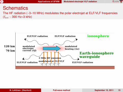
SchematicsThe HF radiation (∼3–10 MHz) modulates the polar electrojet at ELF/VLF frequencies(fmod ∼ 300 Hz–3 kHz)



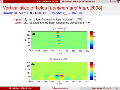
Vertical slice of fields [Lehtinen and Inan, 2008]HAARP HF beam at 3.2 MHz, ERP = 24 MW, fmod = 1875 Hz.

Upper: Bx , formation of upward whistler “column” (∼3 W)Lower: Ez , radiation into the Earth-ionosphere waveguide (∼1 W)

y, km

z,

km

Bx at x=0 km, pT

−400 −300 −200 −100 0 100 200 300 4000

50

100

150

200

250

−20

−10

0

10

20

y, km

z,

km

Ez at x=0 km, mV/m

−400 −300 −200 −100 0 100 200 300 4000

50

100

150

200

250

−0.6

−0.4

−0.2

0

0.2

0.4

(a)

(b)


Applications of SFWM VLF transmitter radiation STANFORDE L E C T R I C A LE N G I N E E R I N G

Outline



3 Conclusions

4 Extra slides



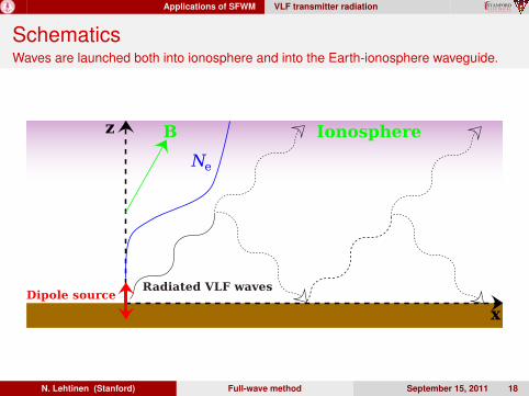
SchematicsWaves are launched both into ionosphere and into the Earth-ionosphere waveguide.



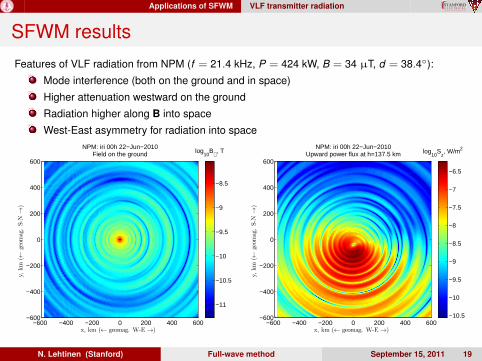
SFWM resultsFeatures of VLF radiation from NPM (f = 21.4 kHz, P = 424 kW, B = 34 µT, d = 38.4◦):

Mode interference (both on the ground and in space)

Higher attenuation westward on the ground

Radiation higher along B into space

West-East asymmetry for radiation into space

x, km (← geomag. W-E→)

y,km

(←geom

ag.S-N→)

NPM: iri 00h 22−Jun−2010Field on the ground

−600 −400 −200 0 200 400 600−600

−400

−200

0

200

400

600

log10

B⊥ , T

−11

−10.5

−10

−9.5

−9

−8.5

x, km (← geomag. W-E→)

y,km

(←geom

ag.S-N→)

NPM: iri 00h 22−Jun−2010Upward power flux at h=137.5 km

−600 −400 −200 0 200 400 600−600

−400

−200

0

200

400

600

log10

Sz, W/m2

−10.5

−10

−9.5

−9

−8.5

−8

−7.5

−7

−6.5



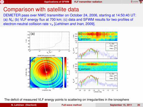
Comparison with satellite dataDEMETER pass over NWC transmitter on October 24, 2006, starting at 14:50:40 UT:(a) Ne; (b) VLF energy flux at 700 km; (c) data and SFWM results for two profiles ofelectron-neutral collision rate νe [Lehtinen and Inan, 2009].

Ew

spectrogram

f, k

Hz (c)

19.2

19.4

19.6

19.8

102

103

104

105

Ew

, µ

V/m

Ew

data

FWM, νen

[V02]

FWM, νen

[H65]

Bw

spectrogram

f, k

Hz

19.2

19.4

19.6

19.8

−24 −22 −20 −18 −16 −14 −12 −10 −810

0

101

102

103

Latitude, deg

Bw

, p

T

Bw

data

FWM, νen

[V02]

FWM, νen

[H65]

100

101

102

103

104

80

85

90

95

100

105

110

Ne, cm

−3

h,

km

(a)

(b)

Longitude, deg

La

titu

de

, d

eg

DEMETER passes over NWC

110 112 114 116 118

−24

−23

−22

−21

−20

−19

−18

−17

dB

re

W/m

2

−95

−90

−85

−80

−75

−70

−65

−60

The deficit of measured VLF energy points to scattering on irregularities in the ionosphere


Applications of SFWM Radiation from lightning STANFORDE L E C T R I C A LE N G I N E E R I N G

Outline



3 Conclusions

4 Extra slides



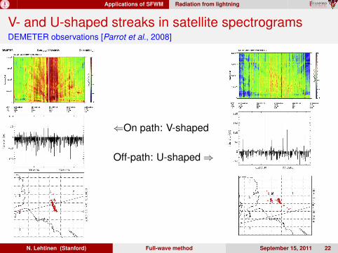
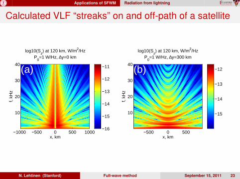
V- and U-shaped streaks in satellite spectrogramsDEMETER observations [Parrot et al., 2008]

⇐On path: V-shaped

Off-path: U-shaped⇒



Calculated VLF “streaks” on and off-path of a satellite

x, km

f, kH

z

log10(Sz) at 120 km, W/m2/Hz

P0=1 W/Hz, ∆y=0 km

(a)

−1000 −500 0 500 1000

10

20

30

40

−16

−15

−14

−13

−12

−11

x, km

f, kH

z

log10(Sz) at 120 km, W/m2/Hz

P0=1 W/Hz, ∆y=300 km

(b)

−500 0 500

10

20

30

40

−15

−14

−13

−12



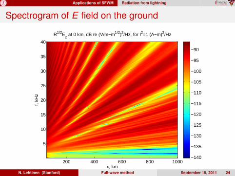
Spectrogram of E field on the ground

x, km

f, kH

zR1/2E

z at 0 km, dB re (V/m−m1/2)2/Hz, for I2=1 (A−m)2/Hz

200 400 600 800 1000

5

10

15

20

25

30

35

40

−140

−135

−130

−125

−120

−115

−110

−105

−100

−95

−90



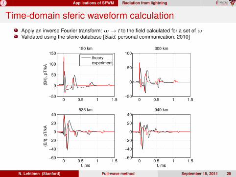
Time-domain sferic waveform calculationApply an inverse Fourier transform: ω→ t to the field calculated for a set ofωValidated using the sferic database [Said, personal communication, 2010]

0 0.5 1 1.5−50

0

50

100

150150 km

(B/I),

pT

/kA

theory

experiment

0 0.5 1 1.5−50

0

50

100300 km

0 0.5 1 1.5−60

−40

−20

0

20

40535 km

t, ms

(B/I),

pT

/kA

0 0.5 1 1.5−60

−40

−20

0

20

40940 km

t, ms


Applications of SFWM Earth-ionosphere waveguide modes STANFORDE L E C T R I C A LE N G I N E E R I N G

Outline



3 Conclusions

4 Extra slides



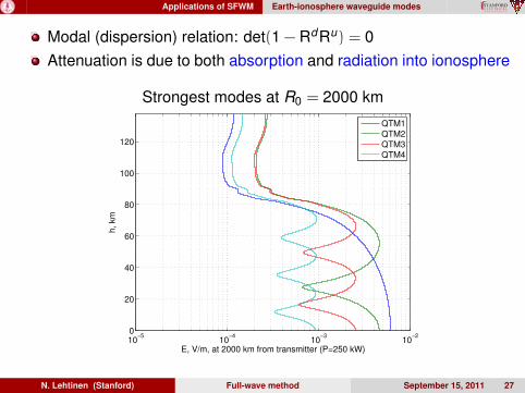
Modal (dispersion) relation: det(1 − RdRu) = 0Attenuation is due to both absorption and radiation into ionosphere

Strongest modes at R0 = 2000 km

10−5

10−4

10−3

10−2

0

20

40

60

80

100

120

E, V/m, at 2000 km from transmitter (P=250 kW)

h,

km

QTM1

QTM2

QTM3

QTM4



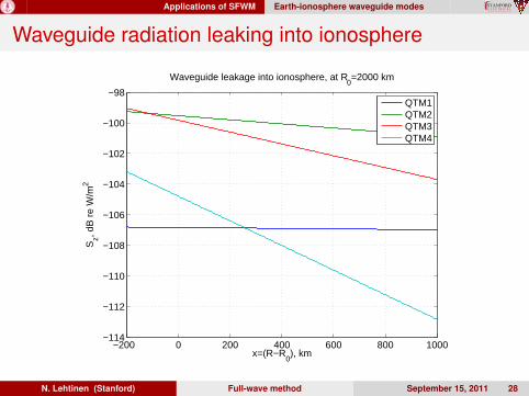
Waveguide radiation leaking into ionosphere

−200 0 200 400 600 800 1000−114

−112

−110

−108

−106

−104

−102

−100

−98

x=(R−R0), km

Sz, d

B r

e W

/m2

Waveguide leakage into ionosphere, at R0=2000 km

QTM1QTM2QTM3QTM4



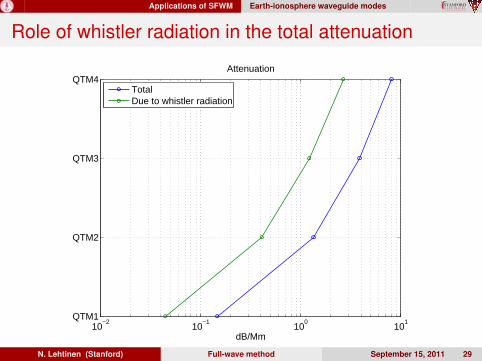
Role of whistler radiation in the total attenuation

10−2

10−1

100

101

QTM1

QTM2

QTM3

QTM4

dB/Mm

Attenuation

TotalDue to whistler radiation


Applications of SFWM Scattering on ionospheric disturbances STANFORDE L E C T R I C A LE N G I N E E R I N G

Outline



3 Conclusions

4 Extra slides



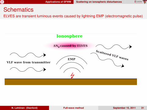
SchematicsELVES are transient luminous events caused by lightning EMP (electromagnetic pulse)



Scattering in Born approximation

Born approximation: neglect the scattered field Es compared tothe incident field E0 inside the scattering regionE0 acting together with the perturbation ∆σ creates currents whichradiate Es



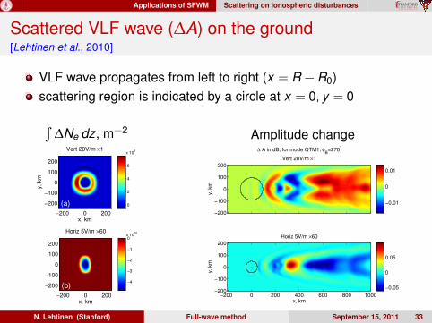
Scattered VLF wave (∆A) on the ground[Lehtinen et al., 2010]

VLF wave propagates from left to right (x = R − R0)scattering region is indicated by a circle at x = 0, y = 0

∫∆Ne dz, m−2

x, km

y, km

Vert 20V/m ×1

(a)

−200 0 200

−200

−100

0

100

200

0

2

4

6

x 109

x, km

Horiz 5V/m ×60

(b)

−200 0 200

−200

−100

0

100

200

−4

−3

−2

−1

0x 10

10

x, km

y, km

Vert 20V/m ×1

(a)

−200 0 200

−200

−100

0

100

200

0

2

4

6

x 109

x, km

Horiz 5V/m ×60

(b)

−200 0 200

−200

−100

0

100

200

−4

−3

−2

−1

0x 10

10

Amplitude change

y,

km

∆ A in dB, for mode QTM1, φB=270

°

Vert 20V/m ×1

−200

−100

0

100

200

−0.01

0

0.01

x, km

y,

km

Horiz 5V/m ×60

−200 0 200 400 600 800 1000−200

−100

0

100

200

−0.05

0

0.05


Conclusions STANFORDE L E C T R I C A LE N G I N E E R I N G

Outline



3 Conclusions

4 Extra slides



Future work

Method of moments instead of Born approximation (moreaccurate)Effects of the Earth’s curvatureLong-distance propagation by using segmented path of a VLFsignal



Summary

We have developed a full-wave method (Stanford FMW) which isstable against “swamping” and easily parallelized. It has been appliedto calculate

Plane wave transport through ionosphereModulated electrojet current radiationRadiation from ground-based transmittersRadiation from lightningEarth-iononsphere waveguide modesScattering on ionospheric disturbances



Acknowledgments

This work was supported byONR grant N0014-09-1-0034NSF grant ATM-0836326DARPA grant HR-0011-10-1-0058DoAF grant FA9453-11-C0011DTRA grant HDTRA-10-1-0115

to Stanford University.



SFWM Bibliography

Lehtinen, N. G., and U. S. Inan (2008), Radiation of ELF/VLFwaves by harmonically varying currents into a stratified ionospherewith application to radiation by a modulated electrojet, J. Geophys.Res., 113, A06301, doi:10.1029/2007JA012911.

Lehtinen, N. G., and U. S. Inan (2009), Full-wave modeling oftransionospheric propagation of VLF waves, Geophys. Res. Lett.,36, L03104, doi:10.1029/2008GL036535.

Lehtinen, N. G., R. A. Marshall and U. S. Inan (2010), Full-wavemodeling of “early” VLF perturbations caused by lightningelectromagnetic pulses, J. Geophys. Res., 115, A00E40,doi:10.1029/2009JA014776.


Extra slides STANFORDE L E C T R I C A LE N G I N E E R I N G

Outline



3 Conclusions

4 Extra slides



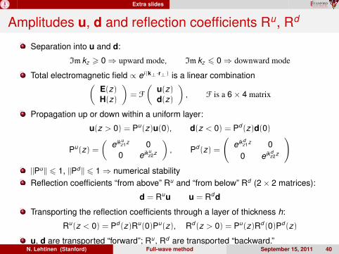
Amplitudes u, d and reflection coefficients Ru, Rd

Separation into u and d:

Im kz > 0⇒ upward mode, Im kz 6 0⇒ downward mode

Total electromagnetic field ∝ ei(k⊥·r⊥) is a linear combination(E(z)H(z)

)= F

(u(z)d(z)

), F is a 6× 4 matrix

Propagation up or down within a uniform layer:

u(z > 0) = Pu(z)u(0), d(z < 0) = Pd (z)d(0)

Pu(z) =(

eikuz1z 00 eiku

z2z

), Pd (z) =

(eikd

z1z 00 eikd

z2z

)||Pu || 6 1, ||Pd || 6 1⇒ numerical stabilityReflection coefficients “from above” Ru and “from below” Rd (2× 2 matrices):

d = Ruu u = Rd d

Transporting the reflection coefficients through a layer of thickness h:

Ru(z < 0) = Pd (z)Ru(0)Pu(z), Rd (z > 0) = Pu(z)Rd (0)Pd (z)

u, d are transported “forward”; Ru , Rd are transported “backward.”N. Lehtinen (Stanford) Full-wave method September 15, 2011 40


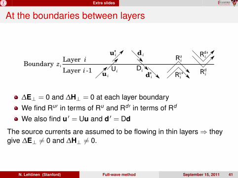
At the boundaries between layers

∆E⊥ = 0 and ∆H⊥ = 0 at each layer boundaryWe find Ru′ in terms of Ru and Rd′ in terms of Rd

We also find u ′ = Uu and d ′ = Dd

The source currents are assumed to be flowing in thin layers⇒ theygive ∆E⊥ 6= 0 and ∆H⊥ 6= 0.



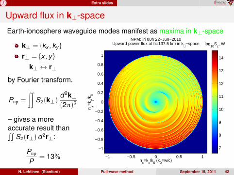
Upward flux in k⊥-space

Earth-ionosphere waveguide modes manifest as maxima in k⊥-space

k⊥ = {kx , ky }

r⊥ = {x , y }k⊥ ↔ r⊥

by Fourier transform.

Pup =

∫∫Sz(k⊥)

d2k⊥(2π)2

– gives a moreaccurate result than∫∫

Sz(r⊥) d2r⊥:

Pup

P= 13%

nx=k

x/k

0 (k

0=w/c)

n y=k y/k

0

NPM: iri 00h 22−Jun−2010Upward power flux at h=137.5 km in k⊥ −space

−1 −0.5 0 0.5 1

−1

−0.8

−0.6

−0.4

−0.2

0

0.2

0.4

0.6

0.8

1

log10

Sz, W

7

8

9

10

11

12

13

14



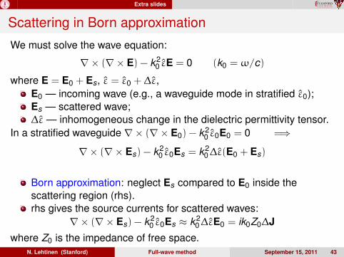
Scattering in Born approximation

We must solve the wave equation:

∇× (∇× E) − k20 ε̂E = 0 (k0 = ω/c)

where E = E0 + Es, ε̂ = ε̂0 + ∆ε̂,E0 — incoming wave (e.g., a waveguide mode in stratified ε̂0);Es — scattered wave;∆ε̂ — inhomogeneous change in the dielectric permittivity tensor.

In a stratified waveguide ∇× (∇× E0) − k20 ε̂0E0 = 0 =⇒

∇× (∇× Es) − k20 ε̂0Es = k2

0∆ε̂(E0 + Es)

Born approximation: neglect Es compared to E0 inside thescattering region (rhs).rhs gives the source currents for scattered waves:

∇× (∇× Es) − k20 ε̂0Es ≈ k2

0∆ε̂E0 = ik0Z0∆Jwhere Z0 is the impedance of free space.


Documents

Full-wave method of calculation of electromagnetic fields ...nlpc.stanford.edu/nleht/Science/talks/2011/ICEAA_Lehtinen_FWM_talk.pdf · Full-wave method of calculation of electromagnetic