Full-Plane STWAVE with Bottom Friction: II. Model Overvie · By Jane McKee Smith. ... The governing equation for steady-state conservation of spectral wave action along a wave ray

PURPOSE: The purpose of this System-Wide Water Resources (SWWRP) Technical Note is to describe the full-plane version of the STWAVE wave generation and transformation model (Smith et al. 2001; Smith 2001; Smith and Smith 2002; and Smith and Zundel 2006). BACKGROUND: STWAVE-FP solves the steady-state conservation of spectral wave action along backward traced wave rays (Smith 2001). The model is used to compute wave transformation (refraction, shoaling, and breaking) and wind-wave generation. The features of the full-plane model include:

• Wave transformation and generation on the full 360-deg plane.

• Option for spatially variable winds and surge.

• Option for spatially constant or spatially variable bottom friction.

• Option for one-dimensional (1-D) wave transformation on lateral boundaries.

• Option for direct input of wave parameters (height, peak period, and mean direction).

• Option for input of plane-beach bathymetry.

• Direction bins no longer restricted to 5 deg.

• X and Y grid cell spacing no longer must be the same. Wave-current interaction is not yet implemented in the full-plane version of the model. GOVERNING EQUATIONS: Refraction and shoaling are implemented in STWAVE by applying the conservation of wave action along backward traced wave rays. Rays are traced in a piecewise manner, from the previous grid column or row. The two-dimensional (2-D) wave spectra are set as input along all grid boundaries. The wave ray is traced back to the previous grid column or row (whichever is encountered first), and the length of the ray segment DR is calculated. Derivatives of depth normal to the wave orthogonal are estimated (based on the orthogonal direction) and substituted into Equation 1 to calculate the wave orthogonal direction at the previous column. The wave orthogonal direction for steady-state conditions is given by (Mei 1989; Jonsson 1990).

ERDC TN-SWWRP-07-5ERDC/CHL CHETN-I-75

August 2007

Full-Plane STWAVE with Bottom Friction: II. Model Overview

By Jane McKee Smith

Report Documentation Page Form ApprovedOMB No. 0704-0188

Public reporting burden for the collection of information is estimated to average 1 hour per response, including the time for reviewing instructions, searching existing data sources, gathering andmaintaining the data needed, and completing and reviewing the collection of information. Send comments regarding this burden estimate or any other aspect of this collection of information,including suggestions for reducing this burden, to Washington Headquarters Services, Directorate for Information Operations and Reports, 1215 Jefferson Davis Highway, Suite 1204, ArlingtonVA 22202-4302. Respondents should be aware that notwithstanding any other provision of law, no person shall be subject to a penalty for failing to comply with a collection of information if itdoes not display a currently valid OMB control number.

1. REPORT DATE AUG 2007 2. REPORT TYPE

3. DATES COVERED 00-00-2007 to 00-00-2007

4. TITLE AND SUBTITLE Full-Plane STWAVE with Bottom Friction: II. Model Overview

5a. CONTRACT NUMBER

5b. GRANT NUMBER

5c. PROGRAM ELEMENT NUMBER

6. AUTHOR(S) 5d. PROJECT NUMBER

5e. TASK NUMBER

5f. WORK UNIT NUMBER

7. PERFORMING ORGANIZATION NAME(S) AND ADDRESS(ES) Engineering Research and Development Center,Vicksburg,MS,39180

8. PERFORMING ORGANIZATIONREPORT NUMBER

9. SPONSORING/MONITORING AGENCY NAME(S) AND ADDRESS(ES) 10. SPONSOR/MONITOR’S ACRONYM(S)

11. SPONSOR/MONITOR’S REPORT NUMBER(S)

12. DISTRIBUTION/AVAILABILITY STATEMENT Approved for public release; distribution unlimited

13. SUPPLEMENTARY NOTES

14. ABSTRACT

15. SUBJECT TERMS

16. SECURITY CLASSIFICATION OF: 17. LIMITATION OF ABSTRACT Same as

Report (SAR)

18. NUMBEROF PAGES

15

19a. NAME OFRESPONSIBLE PERSON

a. REPORT unclassified

b. ABSTRACT unclassified

c. THIS PAGE unclassified

Standard Form 298 (Rev. 8-98) Prescribed by ANSI Std Z39-18

ERDC TN-SWWRP-07-5 ERDC/CHL CHETN-I-75 August 2007

2

DnDd

kdCk

DRDCg 2sinh

−=α (1)

where Cg is group celerity, D is a derivative, α is wave orthogonal direction, R is a coordinate in the direction of the wave ray, C is wave celerity, k is wave number, d is water depth, and n is a coordinate normal to the wave orthogonal. The energy is calculated as a weighted average of energy between the two adjacent grid points in the column and the direction bins. The energy density is corrected by a factor that is the ratio of the 5-deg standard angle band width to the width of the back-traced band to account for the different angle increment in the back-traced ray. The shoaled and refracted wave energy is then calculated from the conservation of wave action along a ray. The governing equation for steady-state conservation of spectral wave action along a wave ray is given by (Jonsson 1990):

ωωαωα SECC

xC g

iig Σ=

∂∂ ),()cos(

)( (2)

where E = wave energy density divided by (ρw g), where ρw is density of water S = energy source and sink terms In a strong opposing current (e.g., ebb currents at an entrance), waves may be blocked by the current. Blocking occurs if there is no solution to the dispersion equation. Or, to state it another way, blocking occurs if the relative wave group celerity is smaller than the magnitude of the opposing current, so wave energy cannot propagate against the current. In deep water, blocking occurs for an opposing current with magnitude greater than one-fourth the deepwater wave celerity without current (0.25 g Ta/(2π), where Ta is the absolute wave period and g is the acceleration of gravity). If blocking occurs, the wave energy is dissipated through breaking. Lai, Long, and Huang (1989) performed laboratory experiments that showed that wave energy can pass through the linear blocking point through nonlinear energy transfers to lower frequencies (which are not blocked). These nonlinear energy transfers are not included in STWAVE. SOURCE AND SINK TERMS Surf-Zone Wave Breaking. The wave-breaking criterion applied in the first version of STWAVE was a function of the ratio of wave height to water depth

kdLH mo tanh1.0max

= (3) where Hmo is the energy-based zero-moment wave height. At a coastal entrance, where waves steepen because of the wave-current interaction, wave breaking is enhanced because of the increased steepening. Smith et al. (1997) performed laboratory measurements of irregular wave

ERDC TN-SWWRP-07-5 ERDC/CHL CHETN-I-75

August 2007

3

breaking on ebb currents and found that a breaking relationship in the form of the Miche criterion (1951) was simple, robust, and accurate (see also Battjes 1982 and Battjes and Janssen 1978). Equation 3 is applied in STWAVE as a maximum limit on the zero-moment wave height. The energy in the spectrum is reduced at each frequency and direction in proportion to the amount of prebreaking energy in each frequency and direction band. Nonlinear transfers of energy to high frequencies that occur during breaking are not represented in the model. Model grid cells where the wave height is limited by Equation 3 are flagged as actively breaking cells. These breaking regions can be visualized in the Surface Water Modeling System (SMS) (Zundel 2005). Wind Input. Waves grow through the transfer of momentum from the wind field to the wave field. The flux of energy, Fin, into the wave field in STWAVE is given by (Resio 1988)

guCF m

w

ain

2*85.0

ρρλ= (4)

where

λ = partitioning coefficient that represents the percentage of total atmosphere to water momentum transfer that goes directly into the wave field (0.75) ρa = density of air ρw = density of water Cm = mean wave celerity u* = friction velocity (equal to the product of the wind speed, U, and the square root of the drag coefficient, CD = .0012+.000025U)

In deep water, STWAVE provides a total energy growth rate that is consistent with Hasselmann et al. (1973). The energy gain to the spectrum is calculated by multiplying the energy flux by the equivalent time for the wave to travel across a grid cell

mgCxt

αβ cosΔ=Δ (5)

where

Δt = equivalent travel time Δx = grid spacing β = factor equal to 0.9 for wind seas ⎯Cg = average group celerity of the spectrum αm = mean wave direction, relative to the grid


4

Wave-Wave Interaction and Whitecapping. As energy is fed into the waves from the wind, it is redistributed through nonlinear wave-wave interaction. Energy is transferred from the peak of the spectrum to lower frequencies (decreasing the peak frequency or increasing the peak period) and to high frequencies (where it is dissipated). In STWAVE, the frequency of the spectral peak is allowed to increase with fetch (or equiva-lently propagation time across a fetch). The equation for this rate of change of fp is given by

( ) ( )7/33/4

*3/71 5

9−

+ ⎥⎥⎦

⎤

⎢⎢⎣

⎡Δ⎟⎟

⎠

⎞⎜⎜⎝

⎛−= t

gu

ffipip ς (6)

where the i and i+1 subscripts refer to the grid column indices within STWAVE and ζ is a dimensionless constant (Resio and Perrie 1989). The energy gained by the spectrum is distributed within frequencies on the forward face of the spectrum (frequencies lower than the peak frequency) in a manner that retains the self-similar shape of the spectrum. Wave energy is dissipated (most notably in an actively growing wave field) through energy transferred to high frequencies and through wave breaking (whitecapping) and turbulent/viscous effects. There is a dynamic balance between energy entering the wave field because of wind input and energy leaving the wave field because of nonlinear fluxes to higher frequencies (Resio 1987; 1988). The energy flux to high frequencies is represented in STWAVE as

)(tanh 4/3

2/932/1

dk

kEg

p

ptotE

ε=Γ (7)

(Resio 1987), where

ΓE = energy flux ε = coefficient equal to 30 Etot = total energy in the spectrum divided by (ρw g), kp = wave number associated with the peak of the spectrum The energy loss from the spectrum is calculated by multiplying the energy flux by the equivalent time for the wave to travel across a grid cell (Δt) (Equation 5) with β equal to 1.0 for the swell portion of the spectrum and 0.9 for the sea portion of the spectrum. This dissipation is only applied in the model if wind input is included. Bottom Friction. STWAVE includes two formulations for bottom friction. The first is the JONSWAP formulation (Hasselmann et al. 1973, Padilla-Hernandez 2001), where the spectral energy loss from bottom friction is formulated as


August 2007

5

),(sinh

12

2

ασ fEkd

cg

S fbf−= (8)

The value of the friction coefficient cf can be specified as a constant over the domain or specified for each STWAVE grid cell. For the JONSWAP bottom friction formulation, cf is specified as Γ/g, where the recommended values of Γ are in the range 0.038 to 0.067 m2/s3 (or cf = 0.004 to 0.007) for sand beds based on experiments in the North Sea. Equation 8 has a weak inverse dependence on water depth (related to the increase in bottom wave orbital velocity as the relative depth, kd, decreases). A Manning formulation is also available in STWAVE (Holthuijsen 2007),

rmsbf ufEkdd

gng

S ),(sinh

12

2

3/1

2

ασ⎟⎟⎠

⎞⎜⎜⎝

⎛−= (9)

where the value of n is specified as input to STWAVE (either spatially constant or variable) and urms is the root-mean-square bottom velocity. With the Manning formulation, bottom friction dissipation has an additional inverse dependence on water depth. Estimates of Manning coefficients are available in most fluid mechanics reference books (e.g., 0.01 to 0.05 for smooth to rocky/weedy channels). The preferred method of specifying cf or n is through calibration with field measurements. Bottom friction in STWAVE has been used to represent dissipation over coral reefs in Hawaii and wetlands in southern Louisiana. Radiation Stress Gradients. Gradients in radiation stress are calculated in STWAVE to provide wave forcing to external circulation models to drive nearshore currents and water level changes (i.e., wave setup and setdown). Wave-driven currents are generally the dominant forcing for sediment transport in the surf zone. Radiation stress tensors are calculated based on linear wave theory:

( ) αααρ dfdkd

kdfEgS wxx ∫∫ ⎥⎦

⎤⎢⎣

⎡−+⎟

⎠⎞

⎜⎝⎛ += 5.01cos

2sinh215.0),( 2 (10)

αααρ dfdkd

kdfEgS wxy ∫∫ ⎥⎦

⎤⎢⎣

⎡⎟⎠⎞

⎜⎝⎛ += 2sin

2sinh215.0

2),(

(11)

( ) αααρ dfdkd

kdfEgS wyy ∫∫ ⎥⎦

⎤⎢⎣

⎡−+⎟

⎠⎞

⎜⎝⎛ += 5.01sin

2sinh215.0),( 2

(12) The gradients in radiation stress are calculated as:

yS

xS xyxx

x ∂∂

−∂

∂−=τ (13)


6

yS

xS yyxy

y ∂∂

−∂

∂−=τ (14)

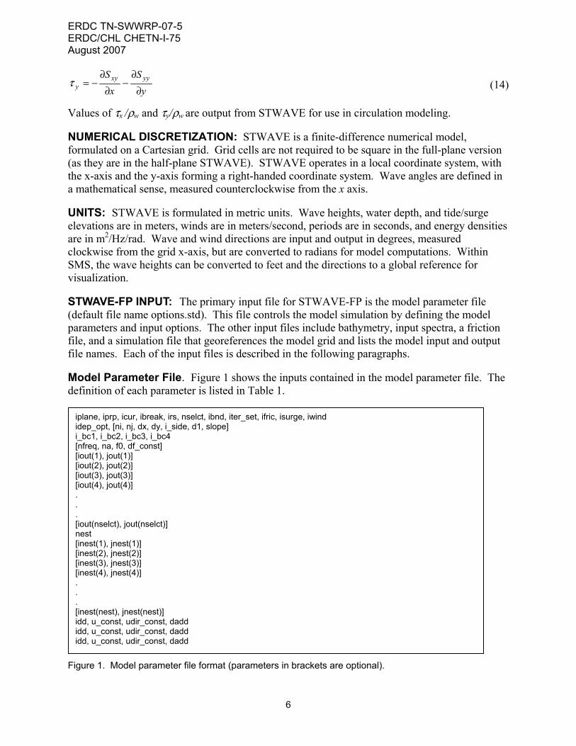
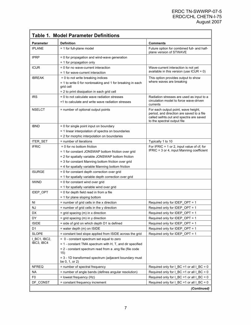
Values of τx /ρw and τy/ρw are output from STWAVE for use in circulation modeling. NUMERICAL DISCRETIZATION: STWAVE is a finite-difference numerical model, formulated on a Cartesian grid. Grid cells are not required to be square in the full-plane version (as they are in the half-plane STWAVE). STWAVE operates in a local coordinate system, with the x-axis and the y-axis forming a right-handed coordinate system. Wave angles are defined in a mathematical sense, measured counterclockwise from the x axis. UNITS: STWAVE is formulated in metric units. Wave heights, water depth, and tide/surge elevations are in meters, winds are in meters/second, periods are in seconds, and energy densities are in m2/Hz/rad. Wave and wind directions are input and output in degrees, measured clockwise from the grid x-axis, but are converted to radians for model computations. Within SMS, the wave heights can be converted to feet and the directions to a global reference for visualization. STWAVE-FP INPUT: The primary input file for STWAVE-FP is the model parameter file (default file name options.std). This file controls the model simulation by defining the model parameters and input options. The other input files include bathymetry, input spectra, a friction file, and a simulation file that georeferences the model grid and lists the model input and output file names. Each of the input files is described in the following paragraphs. Model Parameter File. Figure 1 shows the inputs contained in the model parameter file. The definition of each parameter is listed in Table 1.

Figure 1. Model parameter file format (parameters in brackets are optional).

iplane, iprp, icur, ibreak, irs, nselct, ibnd, iter_set, ifric, isurge, iwind idep_opt, [ni, nj, dx, dy, i_side, d1, slope] i_bc1, i_bc2, i_bc3, i_bc4 [nfreq, na, f0, df_const] [iout(1), jout(1)] [iout(2), jout(2)] [iout(3), jout(3)] [iout(4), jout(4)] . . . [iout(nselct), jout(nselct)] nest [inest(1), jnest(1)] [inest(2), jnest(2)] [inest(3), jnest(3)] [inest(4), jnest(4)] . . . [inest(nest), jnest(nest)] idd, u_const, udir_const, dadd idd, u_const, udir_const, dadd idd, u_const, udir_const, dadd


August 2007

7

Table 1. Model Parameter Definitions Parameter Definition Comments IPLANE = 1 for full-plane model Future option for combined full- and half-

plane version of STWAVE IPRP = 0 for propagation and wind-wave generation

= 1 for propagation only

ICUR = 0 for no wave-current interaction = 1 for wave-current interaction

Wave-current interaction is not yet available in this version (use ICUR = 0)

IBREAK = 0 to not write breaking indices = 1 to write 0 for nonbreaking and 1 for breaking in each grid cell = 2 to print dissipation in each grid cell

This option provides output to show where waves are breaking

IRS = 0 to not calculate wave radiation stresses =1 to calculate and write wave radiation stresses

Radiation stresses are used as input to a circulation model to force wave-driven currents

NSELCT = number of optional output points For each output point, wave height, period, and direction are saved to a file called selhts.out and spectra are saved to the spectral output file

IBND = 0 for single point input on boundary = 1 linear interpolation of spectra on boundaries = 2 for morphic interpolation on boundaries

ITER_SET = number of iterations Typically 1 to 10 IFRIC = 0 for no bottom friction

= 1 for constant JONSWAP bottom friction over grid = 2 for spatially variable JONSWAP bottom friction = 3 for constant Manning bottom friction over grid = 4 for spatially variable Manning bottom friction

For IFRIC = 1 or 2, input value of cf; for IFRIC = 3 or 4, input Manning coefficient

ISURGE = 0 for constant depth correction over grid = 1 for spatially variable depth correction over grid

IWIND = 0 for constant wind over grid = 1 for spatially variable wind over grid

IDEP_OPT = 0 for depth field read in from a file = 1 for plane sloping bottom

NI = number of grid cells in the x direction Required only for IDEP_OPT = 1 NJ = number of grid cells in the y direction Required only for IDEP_OPT = 1 DX = grid spacing (m) in x direction Required only for IDEP_OPT = 1 DY = grid spacing (m) in y direction Required only for IDEP_OPT = 1 ISIDE = side of grid on which depth D1 is defined Required only for IDEP_OPT = 1 D1 = water depth (m) on ISIDE Required only for IDEP_OPT = 1 SLOPE = constant bed slope applied from ISIDE across the grid Required only for IDEP_OPT = 1 I_BC1, IBC2, IBC3, IBC4

= 0 - constant spectrum set equal to zero = 1 - constant TMA spectrum with H, T, and dir specified = 2 - constant spectrum read from a .eng file (file code 15) = 3 - 1D transformed spectrum (adjacent boundary must be 0, 1, or 2)

NFREQ = number of spectral frequency Required only for I_BC =1 or all I_BC = 0 NA = number of angle bands (defines angular resolution) Required only for I_BC =1 or all I_BC = 0 F0 = lowest frequency (Hz) Required only for I_BC =1 or all I_BC = 0 DF_CONST = constant frequency increment Required only for I_BC =1 or all I_BC = 0

(Continued)


8

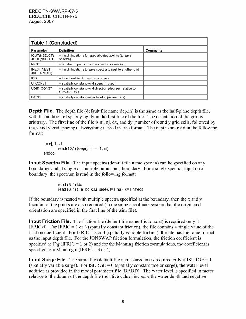
Table 1 (Concluded) Parameter Definition Comments IOUT(NSELCT), JOUT(NSELCT)

= i and j locations for special output points (to save spectra)

NEST = number of points to save spectra for nesting INEST(NEST), JNEST(NEST)

= i and j locations to save spectra to nest to another grid

IDD = time identifier for each model run U_CONST = spatially constant wind speed (m/sec) UDIR_CONST = spatially constant wind direction (degrees relative to

STWAVE axis)

DADD = spatially constant water level adjustment (m)

Depth File. The depth file (default file name dep.in) is the same as the half-plane depth file, with the addition of specifying dy in the first line of the file. The orientation of the grid is arbitrary. The first line of the file is ni, nj, dx, and dy (number of x and y grid cells, followed by the x and y grid spacing). Everything is read in free format. The depths are read in the following format: j = nj, 1, -1 read(10,*) (dep(j,i), i = 1, ni) enddo Input Spectra File. The input spectra (default file name spec.in) can be specified on any boundaries and at single or multiple points on a boundary. For a single spectral input on a boundary, the spectrum is read in the following format: read (8, *) idd read (8, *) ( (e_bc(k,l,i_side), l=1,na), k=1,nfreq) If the boundary is nested with multiple spectra specified at the boundary, then the x and y location of the points are also required (in the same coordinate system that the origin and orientation are specified in the first line of the .sim file). Input Friction File. The friction file (default file name friction.dat) is required only if IFRIC>0. For IFRIC = 1 or 3 (spatially constant friction), the file contains a single value of the friction coefficient. For IFRIC = 2 or 4 (spatially variable friction), the file has the same format as the input depth file. For the JONSWAP friction formulation, the friction coefficient is specified as Γ/g (IFRIC = 1 or 2) and for the Manning friction formulations, the coefficient is specified as a Manning n (IFRIC = 3 or 4). Input Surge File. The surge file (default file name surge.in) is required only if ISURGE = 1 (spatially variable surge). For ISURGE = 0 (spatially constant tide or surge), the water level addition is provided in the model parameter file (DADD). The water level is specified in meter relative to the datum of the depth file (positive values increase the water depth and negative


August 2007

9

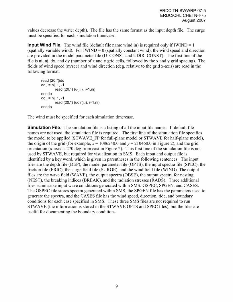
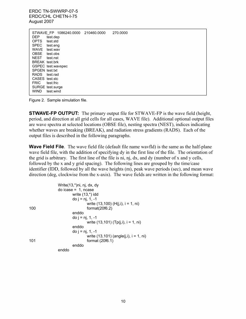
values decrease the water depth). The file has the same format as the input depth file. The surge must be specified for each simulation time/case. Input Wind File. The wind file (default file name wind.in) is required only if IWIND = 1 (spatially variable wind). For IWIND = 0 (spatially constant wind), the wind speed and direction are provided in the model parameter file (U_CONST and UDIR_CONST). The first line of the file is ni, nj, dx, and dy (number of x and y grid cells, followed by the x and y grid spacing). The fields of wind speed (m/sec) and wind direction (deg, relative to the grid x-axis) are read in the following format: read (20,*)idd do j = nj, 1, -1 read (20,*) (u(j,i), i=1,ni) enddo do j = nj, 1, -1 read (20,*) (udir(j,i), i=1,ni) enddo The wind must be specified for each simulation time/case. Simulation File. The simulation file is a listing of all the input file names. If default file names are not used, the simulation file is required. The first line of the simulation file specifies the model to be applied (STWAVE_FP for full-plane model or STWAVE for half-plane model), the origin of the grid (for example, x = 1086240.0 and y = 210460.0 in Figure 2), and the grid orientation (x-axis is 270 deg from east in Figure 2). This first line of the simulation file is not used by STWAVE, but required for visualization in SMS. Each input and output file is identified by a key word, which is given in parentheses in the following sentences. The input files are the depth file (DEP), the model parameter file (OPTS), the input spectra file (SPEC), the friction file (FRIC), the surge field file (SURGE), and the wind field file (WIND). The output files are the wave field (WAVE), the output spectra (OBSE), the output spectra for nesting (NEST), the breaking indices (BREAK), and the radiation stresses (RADS). Three additional files summarize input wave conditions generated within SMS: GSPEC, SPGEN, and CASES. The GSPEC file stores spectra generated within SMS, the SPGEN file has the parameters used to generate the spectra, and the CASES file has the wind speed, direction, tide, and boundary conditions for each case specified in SMS. These three SMS files are not required to run STWAVE (the information is stored in the STWAVE OPTS and SPEC files), but the files are useful for documenting the boundary conditions.


10

Figure 2. Sample simulation file.

STWAVE-FP OUTPUT: The primary output file for STWAVE-FP is the wave field (height, period, and direction at all grid cells for all cases, WAVE file). Additional optional output files are wave spectra at selected locations (OBSE file), nesting spectra (NEST), indices indicating whether waves are breaking (BREAK), and radiation stress gradients (RADS). Each of the output files is described in the following paragraphs. Wave Field File. The wave field file (default file name wavfld) is the same as the half-plane wave field file, with the addition of specifying dy in the first line of the file. The orientation of the grid is arbitrary. The first line of the file is ni, nj, dx, and dy (number of x and y cells, followed by the x and y grid spacing). The following lines are grouped by the time/case identifier (IDD, followed by all the wave heights (m), peak wave periods (sec), and mean wave direction (deg, clockwise from the x-axis). The wave fields are written in the following format: Write(13,*)ni, nj, dx, dy do icase = 1, ncase write (13,*) idd do j = nj, 1, -1 write (13,100) (H(j,i), i = 1, ni) 100 format(20f6.2) enddo do j = nj, 1, -1 write (13,101) (Tp(j,i), i = 1, ni) enddo do j = nj, 1, -1 write (13,101) (angle(j,i), i = 1, ni) 101 format (20f6.1) enddo enddo

STWAVE_FP 1086240.0000 210460.0000 270.0000 DEP test.dep OPTS test.std SPEC test.eng WAVE test.wav OBSE test.obs NEST test.nst BREAK test.brk GSPEC test.wavspec SPGEN test.txt RADS test.rad CASES test.stc FRIC test.fric SURGE test.surge WIND test.wind


August 2007

11

Output Spectra File. The output spectra file (default file name spec.out) is the same as the half-plane model. The spectra are grouped by time/case identifier (IDD) and i and j location. The units of energy density are m2/Hz/rad. The spectra are written in the following format: do nn = 1, nselct ! write to spectral output file write (14, 9003) idd, iout(nn), jout(nn), nn do k = 1, nfreq write (14, 9004) (e(k, l, jout(nn), iout(nn)), l = 1, na) enddo enddo 9004 format (72f8.3) When spectral output points are specified, the wave heights, periods, and directions for those output points are written to a file named selhts.out. The format of this file is: write (12, 9005) idd, iout(nn), jout(nn),H(jout(nn),iout(nn)), Tp(jout(nn),iout(nn)), & angle(jout(nn), iout(nn)) 9005 format(3i10,3f10.2,i10) The output nesting file contains spectra in the same format as the output spectra file, but the header line also contains the x and y coordinates of the output points. Output Breaking File. The output breaking file (default file name break) indicates where waves are breaking with a “1” and nonbreaking with a “0”. This information is used in some sediment transport calculations and may be of interest for safety issues. The breaking file is written in the following format with a file header of nx, ny, dx, and dy: write (22, 9003) idd do j = nj, 1, -1 write (22, *) (ibr(j, i), i = 1, ni) enddo 9003 format (i10, 3i5) Output Radiation Stress Gradient File. The output radiation stress gradient file (default file name radstress) contains the x and y gradients in radiation stress. These gradients are used to calculate wave setup and wave-driven currents in circulation models. The radiation stress gradient file is written in the following format with a file header of nx, ny, dx, and dy: write (18, 9003) idd do j = nj, 1, -1 write (18, *) (wxrs(j, i), wyrs(j, i), i = 1, ni) enddo 9003 format (i10, 3i5) SAMPLE RESULTS: The full-plane version of STWAVE has been applied to studies of Hurricane Katrina in Lake Pontchartrain, Louisiana, under the Interagency Performance Evaluation Task Force (IPET 2006). The domain size for Lake Pontchartrain was 41.6 by 67.4 km with a resolution of 200 m. STWAVE and ADCIRC were loosely coupled by passing storm surge fields from ADCIRC to STWAVE and passing radiation stress fields (to calculate wave setup) from STWAVE to ADCIRC. The input for each grid includes the bathymetry, Manning n


12

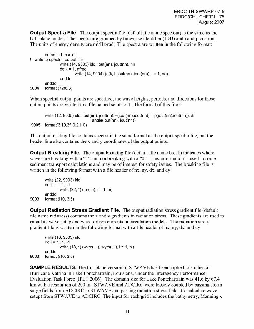
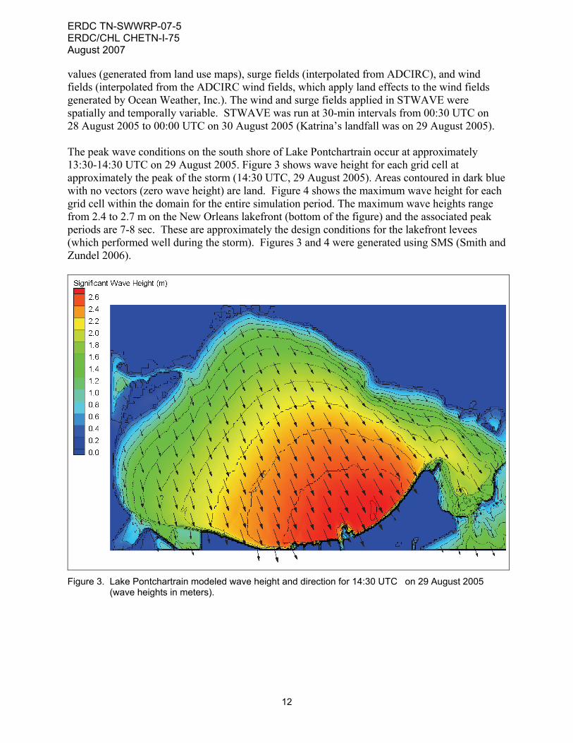
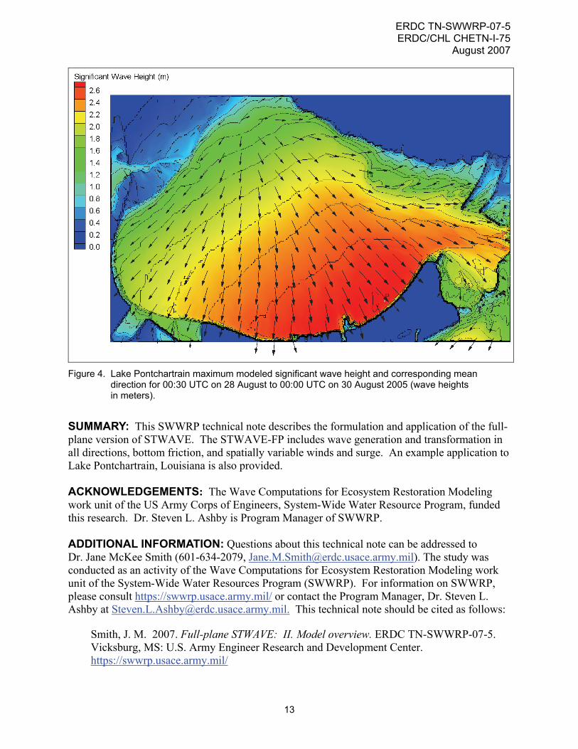
values (generated from land use maps), surge fields (interpolated from ADCIRC), and wind fields (interpolated from the ADCIRC wind fields, which apply land effects to the wind fields generated by Ocean Weather, Inc.). The wind and surge fields applied in STWAVE were spatially and temporally variable. STWAVE was run at 30-min intervals from 00:30 UTC on 28 August 2005 to 00:00 UTC on 30 August 2005 (Katrina’s landfall was on 29 August 2005). The peak wave conditions on the south shore of Lake Pontchartrain occur at approximately 13:30-14:30 UTC on 29 August 2005. Figure 3 shows wave height for each grid cell at approximately the peak of the storm (14:30 UTC, 29 August 2005). Areas contoured in dark blue with no vectors (zero wave height) are land. Figure 4 shows the maximum wave height for each grid cell within the domain for the entire simulation period. The maximum wave heights range from 2.4 to 2.7 m on the New Orleans lakefront (bottom of the figure) and the associated peak periods are 7-8 sec. These are approximately the design conditions for the lakefront levees (which performed well during the storm). Figures 3 and 4 were generated using SMS (Smith and Zundel 2006).

Figure 3. Lake Pontchartrain modeled wave height and direction for 14:30 UTC on 29 August 2005 (wave heights in meters).


August 2007

13

Figure 4. Lake Pontchartrain maximum modeled significant wave height and corresponding mean direction for 00:30 UTC on 28 August to 00:00 UTC on 30 August 2005 (wave heights in meters).

SUMMARY: This SWWRP technical note describes the formulation and application of the full-plane version of STWAVE. The STWAVE-FP includes wave generation and transformation in all directions, bottom friction, and spatially variable winds and surge. An example application to Lake Pontchartrain, Louisiana is also provided. ACKNOWLEDGEMENTS: The Wave Computations for Ecosystem Restoration Modeling work unit of the US Army Corps of Engineers, System-Wide Water Resource Program, funded this research. Dr. Steven L. Ashby is Program Manager of SWWRP. ADDITIONAL INFORMATION: Questions about this technical note can be addressed to Dr. Jane McKee Smith (601-634-2079, [email protected]). The study was conducted as an activity of the Wave Computations for Ecosystem Restoration Modeling work unit of the System-Wide Water Resources Program (SWWRP). For information on SWWRP, please consult https://swwrp.usace.army.mil/ or contact the Program Manager, Dr. Steven L. Ashby at [email protected]. This technical note should be cited as follows:

Smith, J. M. 2007. Full-plane STWAVE: II. Model overview. ERDC TN-SWWRP-07-5. Vicksburg, MS: U.S. Army Engineer Research and Development Center. https://swwrp.usace.army.mil/


14

REFERENCES Battjes, J. A. 1982. A case study of wave height variations due to currents in a tidal entrance. Coast. Engrg. 6: 47-

57.

Battjes, J. A., and J. P. F. M. Janssen. 1978. Energy loss and set-up due to breaking of random waves. Proc. 16th Coast. Engrg. Conf. ASCE. 569-587.

Hasselmann, K., T. P. Barnett, E. Bouws, H. Carlson, D. E. Cartwright, K. Enke, J. A. Ewing, H. Gienapp, D. E. Hasselmann, P. Kruseman, A. Meerburg, P. Muller, D. J. Olbers, K. Richter, W. Sell, and H. Walden. 1973. Measurements of wind-wave growth and swell decay during the Joint North Sea Wave Project (JONSWAP). Deut. Hydrogr. Z., Suppl. A, 8(12): 1-95.

Holthuijsen, L. H. 2007. Waves in ocean and coastal waters. Cambridge: Cambridge University Press. 387 pp.

Interagency Performance Evaluation Task Force (IPET). 2006. Performance evaluation of the New Orleans and southeast Louisiana hurricane protection system, Volume IV – The storm (main text and technical appendices). US Army Corps of Engineers. 1197 pp. https://ipet.wes.army.mil/

Jonsson, I. G. 1990. Wave-current interactions. The sea. Chapter 3, Vol. 9, Part A, B. LeMehaute and D. M. Hanes, ed., New York: John Wiley & Sons, Inc.

Lai, R. J., S. R. Long, and N. E. Huang, N. E. 1989. Laboratory studies of wave-current interaction: kinematics of the strong interaction. Journal of Geophysical Research. 94(C11): 16,201-16,214.

Mei, C. C. 1989. The applied dynamics of ocean surface waves. Singapore: World Scientific Publishing.

Miche, M. 1951. Le pouvoir reflechissant des ouvrages maritimes exposes a l’ action de la houle. Annals des Ponts et Chaussess. 121e Annee: 285-319 (translated by Lincoln and Chevron, University of California, Berkeley, Wave Research Laboratory, Series 3, Issue 363, June 1954).

Padilla-Hernandez, R., and J. Monbaliu. 2001. Energy balance of wind waves as a function of the bottom friction formulation. Coastal Engineering. 43: 131-148.

Resio, D. T. 1987. Shallow-water waves. I: Theory, J. Wtrway., Port, Coast., and Oc. Engrg. ASCE. 113(3): 264-281.

Resio, D. T. 1988. Shallow-water waves. II: Data comparisons,” J. Wtrway., Port, Coast., and Oc. Engrg. ASCE. 114(1): 50-65.

Resio, D. T., and W. Perrie. 1989. Implications of an f—4 equilibrium range for wind-generated waves. J. Phys. Oceanography. 19: 193-204.

Smith, J. M., D. T. Resio and C. L. Vincent, C. L. 1997. Current-induced breaking at an idealized inlet. Proc. Coastal Dynamics ’97. ASCE. 993-1002.

Smith, J. M. and S. J. Smith. 2002. Grid nesting with STWAVE. ERDC/CHL CHETN I-66. Vicksburg, MS: U.S. Army Engineer Research and Development Center. http://chl.wes.army.lmil/library/publications/chetn/.

Smith, J. M. 2001. Modeling nearshore transformation with STWAVE. ERDC/CHL CHETN I-64. Vicksburg, MS: U.S. Army Engineer Research and Development Center. http://chl.wes.army.lmil/library/publications/chetn/.

Smith, J. M., A. R. Sherlock, and D. T. Resio. 2001. STWAVE: Steady-State Wave model user’s manual for STWAVE, Version 3.0. ERDC/CHL SR-01-1, Vicksburg, MS: U.S. Army Engineer Research and Development Center. http://chl.wes.army.mil/research/wave/wavesprg/numeric/wtransformation/downld/erdc-chl-sr-01-11.pdf.

Smith, J. M., and A. K. Zundel, A. K. 2006. Full-Plane STWAVE: I. SMS graphical interface. ERDC/CHL CHETN I-71. Vicksburg, MS: U.S. Army Engineer Research and Development Center. http://chl.wes.army.lmil/library/publications/chetn/.


August 2007

15

Zundel, A. K. 2005. Surface-water Modeling System reference manual – Version 9.0. Provo, UT: Brigham Young University Environmental Modeling Research Laboratory.

NOTE: The contents of this technical note are not to be used for advertising, publication, or promotional purposes.

Citation of trade names does not constitute an official endorsement or approval of the use of such products.

Documents

Full-Plane STWAVE with Bottom Friction: II. Model Overvie · By Jane McKee Smith. ... The governing equation for steady-state conservation of spectral wave action along a wave ray