Embed Size (px)
Citation preview

FU KAI YAP

Representative Models for History Matching and Robust Optimization
By
Fu Kai Yap
in partial fulfilment of the requirements for the degree of
Master of Science in Applied Earth Sciences
at the Delft University of Technology, to be defended publicly on Friday August 26, 2016 at 01:00 PM.
Supervisor: Prof. dr. ir. J.D. Jansen TU Delft E.G.D. de Barros TU Delft
Thesis committee: Dr. O. Leeuwenburgh TNO E.G. Insuasty Moreno TU Eindhoven
An electronic version of this thesis is available at http://repository.tudelft.nl/.

Title : Representative Models for History Matching and Robust Optimization Author(s) : Fu Kai Yap
Supervisors Eduardo Goncalves Dias de Barros MSc [email protected] Prof. dr. ir. Jan Dirk Jansen [email protected] Assessing Committee Dr. Olwijn Leeuwenburgh [email protected] Edwin G. Insuasty Moreno MSc [email protected]
Daily Supervisor PhD Researcher Section : Petroleum Engineering Department of Geoscience and Engineering Faculty of Civil Engineering and Geosciences Delft University of Technology Supervisor Department Head Geoscience & Engineering / Professor of Reservoir Systems and Control Department of Geoscience and Engineering Faculty of Civil Engineering and Geosciences Delft University of Technology Committee Member Researcher/Reservoir Engineer TNO Committee Member PhD Researcher Section : Control Systems Department of Electrical Engineering Eindhoven University of Technology
Copyright © 2016 Section of Petroleum Engineering. All rights reserved. No parts of this publication may be reproduced, stored in a retrieval system, or transmitted, in any form or by any means, electronic, mechanical, photocopying, recording, or otherwise, without the prior written permission of the Section of Petroleum Engineering, Department of Geoscience and Engineering, Delft University of Technology


Acknowledgement
This thesis is the result of supports and contributions from many people.
First and foremost, I would like express my deepest gratitude to my parents for their unconditional love and support throughout my master’s degree in Delft University of Technology. Without them, none if these would be possible.
I would also like to convey my sincerest gratitude to my daily supervisor Eduardo G.D. de Barros for being not only my supervisor but a mentor and most importantly a friend. His guidance and patience has proved to be most needed in the whole process of this thesis. Without him, this thesis would definitely be an arduous journey. Of course not forgetting my gratefulness to Prof. dr. ir. Jan Dirk Jansen for being my supervisor and provides the guidance needed for the completion of this thesis.
A big thank you to Edwin G. Insuasty Moreno for contributing the code for tensor decomposition that was used in this thesis. Also, I would like to thank him and Dr. Olwijn Leeuwenburgh for taking the time and to in read and evaluate this thesis report as a part of the assessing committee.
Last but not least, special thanks to my professors and friends that had helped me to develop and grow professionally and personally in the past 2 years.
This research was carried out within the context of the ISAPP Knowledge Centre. ISAPP (Integrated Systems Approach to Petroleum Production) is a joint project of TNO, Delft University of Technology, ENI, Statoil and Petrobras.
Page | i

Table of Contents Acknowledgement........................................................................................................................................................................................i List of Figures ............................................................................................................................................................................................. iv
List of Tables .................................................................................................................................................................................................v Nomenclature ............................................................................................................................................................................................. vi
Abbreviations ........................................................................................................................................................................................ vi Symbols ................................................................................................................................................................................................... vi
Alphabetical....................................................................................................................................................................................... vi Greek .................................................................................................................................................................................................. vii
Abstract ..........................................................................................................................................................................................................1 1. Introduction..............................................................................................................................................................................................2
1.1 Problem statement ..........................................................................................................................................................................2
1.2 Literature Review ............................................................................................................................................................................2 1.2.1 Parallel Computing..................................................................................................................................................................2
1.2.2 Reduced-O rder Model (ROM)...............................................................................................................................................3 1.2.3 Representative Models...........................................................................................................................................................3
1.3 Hypothesis .........................................................................................................................................................................................3 1.4 Thesis Outline ...................................................................................................................................................................................4
2. Background...............................................................................................................................................................................................5 2.1 Feature and Distance ......................................................................................................................................................................5
2.2 Clustering...........................................................................................................................................................................................5 2.3 Dimensionality Reduction and Projection ................................................................................................................................7
2.3.1 Tensor Decomposition ...........................................................................................................................................................7 2.3.2 Multidimensional Scaling (MDS) .........................................................................................................................................7
2.4 Self-organizing Map (SOM) ...........................................................................................................................................................8 2.5 Robust Optimization .................................................................................................................................................................... 10
2.6 History Matching .......................................................................................................................................................................... 11
3. Methodology .......................................................................................................................................................................................... 14 3.1 Representative Model Selection ............................................................................................................................................... 14
3.1.1 Feature Selection .................................................................................................................................................................. 14 3.1.2 Projection Method ................................................................................................................................................................ 15
3.1.3 Clustering................................................................................................................................................................................ 15 3.1.4 Weighting................................................................................................................................................................................ 15
3.1.5 SOM .......................................................................................................................................................................................... 15 3.2 Validation........................................................................................................................................................................................ 16
3.3 Workflow of Representative Robust Optimization.............................................................................................................. 18
Page | ii

3.4 Workflow of Representative History Matching .................................................................................................................... 19 4. Examples and Results ......................................................................................................................................................................... 20
4.1 Case Studies.................................................................................................................................................................................... 20 4.1.1 2D Model ................................................................................................................................................................................. 20
4.1.2 3D Model ................................................................................................................................................................................. 22 4.2 Robust Optimization Results ..................................................................................................................................................... 23
4.2.1 2D Model ................................................................................................................................................................................. 23
4.2.3 3D Model ................................................................................................................................................................................. 28 4.3 History Matching Results............................................................................................................................................................ 29
4.3.1 2D Model ................................................................................................................................................................................. 29 4.3.2 3D Model ................................................................................................................................................................................. 35
5. Discussion .............................................................................................................................................................................................. 40 6. Conclusion.............................................................................................................................................................................................. 43
References .................................................................................................................................................................................................. 44 Appendix A .....................................................................................................................................................................................................I
Appendix B ................................................................................................................................................................................................... V
Page | iii

List of Figures Figure 1 Workflow of K-means clustering al gorithm ........................................................................................................................6 Figure 2 Workflow of multidimensional scaling .................................................................................................................................8 Figure 3 SOM Kohonen network structure. Light pink denotes the winning node, pink denotes the immediate neighbors and purple denotes further neighbors. (from Kohonen Network - Background Information, 2012) ..............9 Figure 4 Workflow of SOM ..................................................................................................................................................................... 10 Figure 5 Workflow of history matching ............................................................................................................................................. 13 Figure 6 Workflow for selection of representative models (Repr. Select)................................................................................ 14 Figure 7 Representative model selection using SOM...................................................................................................................... 16 Figure 8 Stages of validation ................................................................................................................................................................. 17 Figure 9 Workflow of robust optimization on full ensemble and representative ensemble. (Left) Unoptimized reference (Middle) Representative robust optimization (Right) Full robust optimization reference. ............................. 18 Figure 10 Workflow of history matching on full ensemble and representative ensemble. (Left) Full ensemble history matching (Right) Representative history matching........................................................................................................................ 19 Figure 11: 2D inv erted five-spot configuration ................................................................................................................................ 20 Figure 12 Permeability image of sixteen randomly chosen realizations from simsim model ensemble 50.................... 21 Figure 13 Permeability image of sixteen randomly chosen realizations from channel model ensemble 50 .................. 21 Figure 14 (Left) Reservoir model displaying the position of the injectors (blue) and producers (red). (Right) Six randomly chosen realizations. (from Jansen et al., 2014) ............................................................................................................. 22 Figure 15 Simsim model NPV CDF of 4 ensembles using permeability as feature. (Left) MDS (Right) Tensor decomposition........................................................................................................................................................................................... 23 Figure 16 Simsim model NPV CDF of 4 ensembles using NPV time series as feature. (Left) MDS (Right) Tensor decomposition........................................................................................................................................................................................... 24 Figure 17 Simsim model NPV CDF of 4 ensembles using oil saturation snapshots as feature. (Left) MDS (Right) Tensor decomposition........................................................................................................................................................................................... 24 Figure 18 Simsim model NPV CDF of 4 ensembles using (Left) random selection (Right) oil saturation snapshots with SOM .............................................................................................................................................................................................................. 25 Figure 19 Mean NPV comparison of MDS and tensor decomposition with four ensembles in Simsim model ............... 25 Figure 20 Channel model NPV CDF of 4 ensembles using permeability as feature. (Left) MDS (Right) Tensor decomposition........................................................................................................................................................................................... 26 Figure 21 Channel model NPV CDF of 4 ensembles using NPV time series as feature. (Left) MDS (Right) Tensor decomposition........................................................................................................................................................................................... 26 Figure 22 Channel model NPV CDF of 4 ensembles using oil saturation snapshots as feature. (Left) MDS (Right) Tensor decomposition........................................................................................................................................................................................... 27 Figure 23 Channel model NPV CDF of 4 ensembles using (Left) random selection (Right) oil saturation snapshots with SOM .............................................................................................................................................................................................................. 27 Figure 24 NPV comparison of MDS and Tensor with four ensembles in Channel model ..................................................... 28 Figure 25 Egg Model robust optimization results. .......................................................................................................................... 29 Figure 26 Permeability results of history matching using MDS. (Top) Simsim Model (Bottom) Channel Model .......... 29 Figure 27 Simsim Model field production data of representative ensemble using all oil saturation snapshots at time 1,500 days. Red is oil and blue is water. (Left) The priori (Right) The posterior ................................................................... 30 Figure 28 Simsim Model field production data of posterior of 10 representative realizations using MDS and all oil saturation snapshots at v arious history matching time. Red is oil and blue is water............................................................ 31 Figure 29 Simsim Model field production data of posterior of 10 representative realizations using MDS and oil saturation snapshots up to specified history matching time. Red is oil and blue is water ................................................... 31 Figure 30 Simsim Model NPV comparison of 10 representative realizations using MDS. Repr prior all and repr post all are selected using all oil saturation snapshots whereas repr prior and repr post are selected using oil saturation snapshots up to the history matching time. (Left) The prior NPV CDF plot. (Right) The posterior NPV CDF plot. ....... 32 Figure 31 Channel Model field production data of representative ensemble using all oil saturation snapshots at time 1,500 days. Red is oil and blue is water. (Left) The prior (Right) The posterior..................................................................... 33
Page | iv

Figure 32 Channel Model field production data of posterior of 10 representative realizations using MDS and all oil saturation snapshots at v arious history matching time. Red is oil and blue is water............................................................ 33 Figure 33 Channel Model field production data of posterior of 10 representative realizations using MDS and oil saturation snapshots up to specified history matching time. Red is oil and blue is water ................................................... 34 Figure 34 Channel Model NPV comparison of 10 representative realizations using MDS. Repr prior all and repr post all are selected using all oil saturation snapshots whereas repr prior and repr post are selected using oil saturation snapshots up to the history matching time. (Left) The prior NPV CDF plot. (Right) The posterior NPV CDF plot. ....... 34 Figure 35 Examples of history matched layer 4 of Egg Model permeability field using (Top) MDS (Bottom) Tensor decomposition. .......................................................................................................................................................................................... 35 Figure 36 Egg Model water (blue) and oil (red) production rates. Representative ensembles selected using MDS. .... 36 Figure 37 Egg Model injector rates of representative ensembles using MDS as projection method. (Left) Prior (Right) Posterior ..................................................................................................................................................................................................... 36 Figure 38 Egg Model water (blue) and oil (red) production rates. Representative ensembles selected using tensor decomposition. .......................................................................................................................................................................................... 37 Figure 39 Egg Model injector rates of representative ensembles using tensor decomposition as projection method. (Left) Prior (Right) Posterior ................................................................................................................................................................ 37 Figure 40 Normalized sum of square error at 1,800 days of field oil and water production rates to the truth. ............ 38 Figure 41 Egg Model history matching prior and posterior final NPV CDF using full ensemble and representative ensemble selected using MDS and tensor decomposition. ............................................................................................................ 39 Figure 42 Simsim model NPV CDF of 6 additional ensembles using permeability as feature. (Left) MDS (Right) Tensor decomposition...............................................................................................................................................................................................I Figure 43 Simsim model NPV CDF of 6 additional ensembles using NPV time series as feature. (Left) MDS (Right) Tensor decomposition ................................................................................................................................................................................I Figure 44 Simsim model NPV CDF of 6 additional ensembles using oil saturation snapshots as feature. (Left) MDS (Right) Tensor decomposition ................................................................................................................................................................ II Figure 45 Simsim model NPV CDF of 6 additional ensembles using (Left) Random selection (Right) oil saturation snapshots with SOM................................................................................................................................................................................... II Figure 46 Channel model NPV CDF of 6 additional ensembles using permeability as feature. (Left) MDS (Right) Tensor decomposition............................................................................................................................................................................................ III Figure 47 Channel model NPV CDF of 6 additional ensembles using NPV time series as feature. (Left) MDS (Right) Tensor decomposition ............................................................................................................................................................................. III Figure 48 Channel model NPV CDF of 6 additional ensembles using oil saturation snapshots as feature. (Left) MDS (Right) Tensor decomposition ............................................................................................................................................................... IV Figure 49 Channel model NPV CDF of 6 additional ensembles using (Left) Random selection (Right) oil saturation snapshots with SOM ................................................................................................................................................................................. IV
List of Tables Table 1: Reservoir Properties for 2D Model...................................................................................................................................... 20 Table 2 Reservoir properties for Egg Model ..................................................................................................................................... 22
Page | v

Nomenclature Abbreviations AI Artificial intelligence ANN Artificial neural network CDF Cumulative distribution function CLRM Closed-loop reservoir management KS test Kolmogorov-Smirnov Test MDS Multidimensional scaling NPV Net present value PCA Principal Component Analysis POD Proper orthogonal decomposition Post. Posterior Repr. Representative ROM Reduced-order model SOM Self-organizing Map SSE Sum of squared error SVD Singular value decomposition TPWL Trajectory piecewise l inearization UQ Uncertainty quantification VOI Value of information
Symbols Alphabetical 𝐴𝐴 Amplitude of neighborhood adaptation 𝐂𝐂 Covariance matrix C Cluster set 𝑐𝑐 K-means centroid 𝐃𝐃 Dissimilarity matrix 𝐃𝐃� Projected dissimilarity matrix 𝑑𝑑l Projected distance in low dimensional space �̂�𝑑 Monotonic transformation of dissimilarity 𝐝𝐝𝑜𝑜𝑜𝑜𝑜𝑜 Observation data vector 𝑒𝑒2 Squared error criterion 𝑖𝑖𝑖𝑖𝑖𝑖 SOM iteration number 𝐽𝐽 Objective function 𝐾𝐾 Number of clusters 𝑀𝑀 Number of feature data dimension 𝐌𝐌 Ensemble parameter matrix 𝐌𝐌𝑓𝑓𝑓𝑓𝑓𝑓𝑓𝑓 Full ensemble parameter matrix 𝐌𝐌𝑟𝑟𝑟𝑟𝑟𝑟𝑟𝑟 . Representative ensemble parameter matrix 𝐌𝐌𝑟𝑟𝑟𝑟𝑖𝑖𝑜𝑜𝑟𝑟 Prior ensemble parameter matrix 𝐌𝐌𝑟𝑟𝑜𝑜𝑜𝑜𝑖𝑖 . Posterior ensemble parameter matrix 𝐦𝐦 Model parameters vector 𝐦𝐦𝑓𝑓𝑓𝑓𝑓𝑓𝑓𝑓 Full model parameters vector 𝐦𝐦𝑟𝑟𝑟𝑟𝑟𝑟𝑟𝑟. Representative model parameters vector 𝐦𝐦𝑟𝑟𝑟𝑟𝑖𝑖𝑜𝑜𝑟𝑟 Prior model parameter 𝐦𝐦�𝑟𝑟𝑟𝑟𝑖𝑖𝑜𝑜𝑟𝑟 Projected prior model parameter
Page | vi

𝐦𝐦𝑟𝑟𝑜𝑜𝑜𝑜𝑖𝑖 . Posterior model parameter vector 𝐦𝐦�𝑟𝑟𝑜𝑜𝑜𝑜𝑖𝑖 . Projected posterior model parameter vector 𝑁𝑁 Number of Kohonen nodes 𝑁𝑁𝑟𝑟𝑟𝑟𝑟𝑟𝑟𝑟 Number of representative realizations 𝑅𝑅 Number of realizations 𝐒𝐒 3D tensor 𝑠𝑠 Stress function 𝐮𝐮 Control input vector 𝐰𝐰 Kohonen weight vector 𝐰𝐰𝑟𝑟𝑟𝑟𝑟𝑟𝑟𝑟 Representative Realizations weight vector 𝐗𝐗 2D grid property matrix 𝐱𝐱 State vector
Greek 𝛼𝛼 Monotonic decreasing learning coefficient 𝛿𝛿 Pairwise distance (dissimilarity) 𝚯𝚯 Feature data matrix 𝚯𝚯� Projected feature data matrix 𝚯𝚯𝑜𝑜𝑓𝑓𝑜𝑜 Sub ensemble feature data matrix 𝛉𝛉 Feature data vector 𝜇𝜇 Mean 𝜇𝜇𝑁𝑁𝑁𝑁𝑁𝑁 Ensemble mean 𝜎𝜎 Standard deviation 𝝋𝝋 1st orthonormal basis functions (vectors) 𝚿𝚿 2nd orthonormal basis functions (vectors) 𝝌𝝌 3rd orthonormal basis functions (vectors)
Page | vii

Abstract
Reservoir management has been widely implemented in the petroleum industry to attain the best performance out of the asset. Highly efficient computer-assisted reservoir management is getting more common and therefore enabling the incorporation of ensembles to provide uncertainty quantification (UQ). Closed-loop reservoir management (CLRM) further enhances reservoir management by combining robust optimization and history matching while accounting for UQ. However, CLRM workflow is very computationally intensive. In addition, value of information (VOI) workflows that make use of CLRM framework are currently unfeasible mainly due to multiplication of the already immense computational cost required. Therefore, this thesis proposes a method to select representative models forming a reduced ensemble that can replace the full ensemble in robust optimization and history matching.
We use clustering algorithm to select the representative models. Features were extracted based on various model parameters and projected into lower dimensional space using ordination techniques. Different number of representative models were investigated to explore the performance and discover the minimal number of models required in a representative ensemble.
The method is tested in two simple 2D models and in a larger 3D Model. The results showed a very promising future for representative ensembles to be applied in robust optimization where an order of magnitude speedup is estimated. Whereas the implementation of representative ensembles in history matching may require higher number of representative models, although achieving a commendable result. Depending on the size of original ensemble, using reduced ensemble can greatly decrease the computational cost associated with optimization and simulation while providing very comparable results to using full ensemble.
Page | 1

Chapter 1: Introduction
1. Introduction 1.1 Problem statement In the exploration and production sector, companies have to make difficult decisions regarding the development strategies for their assets. The fact that every reservoir is the only one of its kind means that there is no room for experiments to be carried out to determine the best development strategy. Because of that, numerical simulations are extensively used in reservoir engineering to characterize the reservoirs and predict their production. In essence, simulation models are populated with parameters derived from all the available data from the reservoir (e.g., lithological and pore fluid data). Due to the limited knowledge of the true reservoir, it is common to generate more than one interpretation from collected field data, which, in most cases, results in several models of the subsurface.
To extensively account for uncertainty in reservoir model parameters, an ensemble of reservoir realizations is employed in most modern reservoir management workflows. Uncertainty quantification (UQ) is of major interest in the petroleum industry where quantitative characterization and assessment of uncertainties are paramount to reduce the risk for all field development. While considering an ensemble of models allows to better define, ideally, all possible reservoir characteristics, it leads to additional demand in computational cost to achieve optimal reservoir management.
Closed-loop reservoir management (CLRM) framework combines model-based life-cycle optimization and computer-assisted history matching (Jansen et al., 2009) to maximize the reservoir performance (i.e., recovery or financial measures) and obtain the optimal strategy for reservoir management. In a nutshell, CLRM makes use of data collected throughout the reservoir life-cycle to update the reservoir models which, in turn, improve the optimization of the field production strategy.
In combination with UQ by using an ensemble of model realizations, the computational cost of CLRM workflows increases significantly. Workflows to assess value of information (VOI) in CLRM with UQ as proposed by Barros et al. (2016a) further multiply the cost of computation by order of tens or hundreds, making real-field implementation unfeasible with the current advancement in computational power. Therefore, some alternatives are needed to reduce the computational cost to an acceptable range.
1.2 Literature Review Since the main barrier for a wide implementation of VOI assessment is the computational cost; techniques for accelerating these workflows need to be found. Three main categories of solutions for speeding-up simulations are identified. The first one corresponds to the ‘brute-force’ approach by increasing computing power to solve larger problems. The second method seeks to speedup simulations by using surrogate models (i.e., approximate or proxy models). And the third one aims at reducing the number of required simulations directly by approximating UQ (i.e., considering few representative models).
1.2.1 Parallel Computing This may be the simplest approach where the great amount of simulations is simply solved by increasing the computing power. The advancement of ever faster processors and the advent of parallel computing have made this approach rather attractive for companies that are well-funded.
Despite showing many advantages, the development of software for parallel computing can be very complex. Ouenes et al. (1995) and Salazar et al. (1996) have shown that it is possible to have parallel computers and a network of workstations to run simulations without modification by using Parallel Virtual Machine. Schiozer (1999) introduced Module for Parallel Simulations which uses Parallel Virtual Machine to distribute the simulations efficiently by taking into account the speed and dynamic characteristics of each machine. He also concluded that, by using Module for Parallel Simulations in parallel computing, it is possible to reduce the cost of hardware by automating the simulation process and taking advantage of idle workstations.
Page | 2

Chapter 1: Introduction
1.2.2 Reduced-Order Model (ROM) The aim of ROM is to create a simpler model that can to an extent accurately reproduce the output of a simulator. A good ROM should be accurate while requiring significantly less computational cost than the full-order model.
One approach is implemented by reconstructing a grid based numerical model into a coarser grid model. This approach is considered as grid-based reduced-order model and can be constructed using either upscaling or multiscale method. The former have the disadvantage of losing finer grid resolution while the latter retain information on finer scale commonly with dual-grid methods that are coupled by the prolongation (coarse to fine) and restriction (fine to coarse) operators. However, multiscale methods require extra computation of the operators before simulation, thus limiting the potential for speedup of our workflows. Krogstad et al. (2011) have shown that using multiscale methods can achieve a speedup of an order magnitude in water flooding optimization.
Another approach is to use snapshots of time-variant problems to create basis functions in order to have a reduced model. This method utilizes proper orthogonal decomposition (POD) to calculate the basis functions. However, the large number of variable changes in history matching heavily diminishes the speedup of POD when applied in reservoir simulation. He (2013) utilized trajectory piecewise linearization (TPWL) in conjunction with POD for model-order reduction in history matching whereas Hewson (2015) tested on ensemble-based robust optimization. This method achieved an order of magnitude acceleration in terms of simulation time although it sacrifices the accuracy of the results. However, when accounting for the preprocessing required to build the proxy models, the application of POD-TPWL in CLRM workflow achieved a speedup that is much lower than in simulation alone.
Insuasty et al. (2015a) introduced tensor-based ROM using tensor decomposition and representations of flow characteristics to quantify the features of flow simulations. They compared the tensor approach to POD for adjoint-based optimization where the tensor approach achieved better financial performance. They also showed that tensor models provide higher approximation accuracy over classical POD models, although the computational gain is low.
1.2.3 Representative Models Sarma et al. (2013) proposed a method for selecting representative realizations for UQ. They claim that their minimax method is able to efficiently select a few reservoir models from a large ensemble by matching target percentiles of multiple output responses while obtaining maximally different models in the parameter uncertainty space. The idea behind the minimax method is to select representative models that are statistical representative while maximizing the spread in the parameter uncertainty space. The authors also claimed that the solution from minimax is generally better than clustering and that the computation is orders of magnitude faster. Although their method ensures good spread of selected models in parameter and output spaces, Sarma et al. (2013) did not address the effectiveness of using selected representative models in optimization or history matching workflows.
Insuasty et al. (2015b) proposed a measure of dissimilarity that is based on reservoir flow patterns in numerical simulation using flow variables such as oil saturation. They suggest that, by applying tensor decomposition on spatial-temporal representation of the reservoir flow patterns (e.g., snapshots of the temporal evolution of oil saturation distribution), the structure of the flow data can be preserved, which allows to better determine dominant flow patterns. Tensor decomposition provides a dissimilarity measure that offers low dimension data and thus easier to be used for model classification. Clustering of realizations from an example ensemble were compared in the paper, the results showed this method is able to provide better defined clusters compared to singular value decomposition (SVD. Insuasty et al. (2015b) showed that, by reducing the number of realizations from 1,000 to 50 realizations in flow-relevant ensemble, it is possible to obtain similar optimal production strategy and yield similar final net present value (NPV) distribution.
1.3 Hypothesis While an ensemble can more effectively quantify uncertainties, it is arguably unnecessary for robust optimization (Section 2.5 Robust Optimization) and history matching (Section 2.6 History Matching) procedures to require hundreds of model realizations. By grouping similar realizations and selecting representative realizations for each group we can greatly reduce the ensemble size as well as directly decrease the computational cost of our workflows. Many studies have used representative ensemble for UQ, but very few have focused on using representative ensembles for
Page | 3

Chapter 1: Introduction
optimization. Of course, the implementation of representative ensembles need to have similar effect on robust optimization and history matching which are the main principles in CLRM. This thesis investigates whether, with clever selection of representative realizations to represent the original full ensemble, robust optimization and history matching can be carried out more efficiently while performing close to the full ensemble. This thesis also makes an attempt to understand the fundamentals of selecting good representative models and, more importantly, to determine the bare minimum of representative models needed for an accurate representation of the full ensemble.
1.4 Thesis Outline In Chapter 2. Background we discuss about the fundamentals of robust optimization, history matching and techniques required for representative model selection. Chapter 3. Methodology introduces the procedure used in order to select and construct the representative ensembles followed by techniques on validating the performance. Chapter 4. Examples describes the case study examples and presents the results on the performance of representative ensemble. Chapter 5. Discussion presents the summary and challenges faced using the proposed method followed by various reasonings and future works that may to improve the method. Finally, Chapter Conclusion wrap up by presenting the essential findings of the thesis.
Page | 4

Chapter 2: Background
2. Background 2.1 Feature and Distance Feature describes the property selected in order to distinguish between realizations. The feature data matrix 𝚯𝚯 =[𝛉𝛉1 𝛉𝛉2… 𝛉𝛉𝑅𝑅] contains the feature data vectors 𝛉𝛉 of the individual realizations, which have dimension 𝑀𝑀 . 𝚯𝚯 can be used for selecting representative realizations.
Here ‘distances’ are measures of dissimilarity between realizations. They are always defined as pairwise distances in terms of any form of feature of a reservoir. In petroleum engineering, the distances can be generally categorized into static and dynamic. Static distances are calculated from initial grid based properties or parameters (e.g., permeability and initial oil saturation). Dynamic distances, on the other hand, require simulated properties (e.g., NPV, streamlines and oil production rates). Suzuki et al. (2008) and Caers et al. (2010) have used permeability as a distance measure to differentiate model realizations based on geological features. Van Essen et al. (2009) and Jansen et al. (2009) have shown that, although reservoir models might have different geological properties, they may generate the same NPV under individually optimized strategies. Scheidt and Caers (2009) and Scheidt et al. (2011) use the cumulative oil and water production rates as the dissimilarity measures to assess the flow uncertainty. Park and Caers (2007), Scheidt et al. (2009) and Scheidt and Caers (2009) used streamline simulators to produce fast characterization of cumulative oil and water production to distinguish models.
The distance measures can be computed in multiple ways (e.g., Euclidean, Manhattan, and Minkowski). The Euclidean distance, defined as the ‘straight-line’ distance between two points in Euclidean space, is the one used in this thesis. It is formulated as
Equation 1
𝛿𝛿𝑖𝑖𝑖𝑖 = ��𝛉𝛉𝑖𝑖 − 𝛉𝛉𝑖𝑖 �2
,
where 𝛿𝛿𝑖𝑖𝑖𝑖 is the pairwise distance between realization 𝑖𝑖 and 𝑗𝑗 in terms of the selected feature. Given a set of 𝑅𝑅 realizations, D is be the dissimilarity matrix of 𝑅𝑅 × 𝑅𝑅 containing the distance between two realizations 𝛿𝛿𝑖𝑖𝑖𝑖. 𝛿𝛿𝑖𝑖𝑖𝑖 is be 0 when i=j as there is no dissimilarity among itself and 𝛿𝛿𝑖𝑖𝑖𝑖 is equal to 𝛿𝛿𝑖𝑖𝑖𝑖 .
Equation 2
𝐃𝐃 = �𝛿𝛿11 ⋯ 𝛿𝛿1𝑁𝑁⋮ ⋱ ⋮𝛿𝛿𝑁𝑁1 ⋯ 𝛿𝛿𝑁𝑁𝑁𝑁
� .
2.2 Clustering One of the most obvious ways of finding representative models is to group them according to some criteria and select a model out of each group. Clustering analysis is a family of techniques used to partition a set of similar points (i.e. objects or observations) into clusters. Cluster analysis aims to unveil the internal organization of a dataset by detecting the structure within the data in the form of clusters. The goal of clustering is to categorize similar data together. Therefore it is useful for reducing the amount of data. Such uses of grouping are pervasive in how humans process information. Cluster analysis using numerical methods were introduced in biological classifications (Jardine and Sibson, 1971; Sneath and Sokal, 1973) and have been used in pattern recognition (Anderberg, 2014), image processing (Jain and Flynn, 1996), machine learning (Arabie and Hubert, 1996) and many other domains such as psychology, geology, marketing and archaeology (Jain et al. 2009).
At the top level of cluster analysis classification, there is an important distinction between hierarchical and partitional approaches. Hierarchical clustering produces nested groupings based on criteria for merging or splitting clusters. The nested groupings in hierarchical clustering can thus be presented in a dendrogram. On the other hand, partitional clustering separates the points into exclusive clusters by optimizing a defined criterion function. The most common criterion function used is the squared error criterion which performs well with compact and isolated clusters (Jain et al., 2009). The squared error criterion is defined by
Page | 5

Chapter 2: Background
Equation 3
𝑒𝑒2 = ���𝑥𝑥𝑖𝑖𝑖𝑖 − 𝑐𝑐𝑖𝑖�
2
𝑛𝑛𝑗𝑗
𝑖𝑖 =1
𝐾𝐾
𝑖𝑖=1
,
where 𝑥𝑥𝑖𝑖𝑖𝑖 is the 𝑖𝑖𝑖𝑖ℎ point in cluster 𝑗𝑗, 𝑐𝑐𝑖𝑖 is the centroid of cluster 𝑗𝑗 and 𝐾𝐾 is the predefined number of clusters and 𝑛𝑛𝑖𝑖
is the nth point in cluster 𝑗𝑗.
Figure 1 Workflow of K-means clustering algorithm
K-means clustering is the simplest and most common clustering algorithm (McQueen, 1967; Caers, 2011) that employ the squared error criterion. The name K-means comes from the technique itself whereby it tries to partition data into k clusters of which each data point belongs to the cluster with the nearest mean (i.e., the centroid). Figure 1 illustrates the workflow of K-means clustering algorithm where it starts with predefined k number of randomize centroid placement. Next, all points are assigned to the nearest centroid. The mean of each cluster is then calculated and the centroid is reassigned to the new mean. The criterion function is then calculated and reassignment of all points to new centroids is carried out if convergence is not met. Typically we minimize some measure of dissimilarity in the samples within each cluster (i.e., intra-cluster distance), while maximizing the dissimilarity between clusters (i.e., inter-cluster distance). With user predefined number 𝐾𝐾 sets of cluster C𝑘𝑘 , where 𝑘𝑘 = 1, 2, … ,𝐾𝐾 , of which individual C𝑘𝑘 contains 𝑛𝑛𝑘𝑘 unique indices. When using K-means clustering on a fixed indices dataset and applying squared error criterion (Equation 3), K-means clustering can then be stated as an optimization problem defined as
Equation 4
C𝑜𝑜𝑟𝑟𝑖𝑖 = arg minC
� �‖𝑥𝑥𝑖𝑖 − 𝑐𝑐𝑘𝑘‖2 ,𝑖𝑖∈C𝑘𝑘
𝐾𝐾
𝑘𝑘=1
where 𝑐𝑐𝑘𝑘 = 1𝑛𝑛𝑘𝑘∑ 𝑥𝑥𝑖𝑖𝑖𝑖∈C𝑘𝑘
. In a sentence, K-means clustering is an iterative process which partitions the data by
minimizing the within cluster sum of point-to-cluster centroid distances over all clusters. Many clustering algorithms suffer from inefficiency when performed on high dimensional data due to the inherent sparsity of data: as the number of dimensions increases, the distance measures becomes equidistant (Berchtold et al., 1997; Parsons et al., 2004). Therefore, dimensionality reduction is recommended to treat the high dimensional data before clustering.
Page | 6

Chapter 2: Background
Another major issue with K-means algorithm is the sensitivity to the initial randomized partition that may lead to local minimum convergence. However, this problem can be mitigated by repeating the clustering process with different random seeds. Many variant of K-means clustering have been introduced to improve and add new attributes. Arthur and Vassilvitskii (2007) proposed a useful variant named K-means++ which chooses the initial values that try to spread out clusters’ centroids. Shindler (2008) pointed out that K-means++ is able to overcome some of the problems associated with defining initial clusters’ centroids compared to K-means algorithm. In general, K-means clustering is a robust way for grouping seemingly unrelated data spread and is widely used in engineering to group scattered data points.
2.3 Dimensionality Reduction and Projection High dimensional data suffer from a few drawbacks. The most inconvenient one concerns the data containing excessive and often unneeded information. When operations are carried out on high dimensional data, unwanted effects such as data over-fitting and suboptimal search are likely to occur, besides increasing the computational cost. The goal of projections is to represent the parameters in lower dimensional space that preserve certain properties of the data structure as faithfully as possible. Therefore, projections can be very helpful in providing a better dataset for further operations. Aggarwal et al. (1999) have shown that the projection of high dimensional data spaces into low dimension subspaces leads to improved clustering results.
2.3.1 Tensor Decomposition One projection method is proposed by Insuasty et al. (2015) where dimension reduction is achieved through tensor decomposition. Tensor decomposition is strongly related to principal component analysis (PCA) or singular value decomposition (SVD). While PCA and SVD are also applicable in this context, tensor decomposition is able to reduce the dimension while honoring the original data structure and correlations (e.g., spatial and temporal). These structures are often lost with data vectorization needed in PCA and SVD techniques. For example on an ensemble of 2D models, rather than vectorization, tensor decomposition operates by constructing a 3D tensor. The first two dimension correspond to the original spatial structure of the feature data and the third dimension to the realization number (i.e., the uncertainty dimension). More dimensions, such as time, may be included by taking snapshots of the feature property. According to Insuasty et al. (2015), tensor decomposition is able to compress large datasets while having minimal approximation and reconstruction error.
Consider a 2D reservoir model with 2D grid properties matrix 𝐗𝐗 (size 𝐼𝐼 × 𝐽𝐽) at different time snapshot 𝐾𝐾 stacked into 3D tensor 𝐒𝐒 = [𝐗𝐗1,𝐗𝐗2, … ,𝐗𝐗𝐾𝐾 ]. Tensor 𝐒𝐒 can be decomposed as
Equation 5
𝐒𝐒� = ��� 𝜎𝜎𝑖𝑖𝑖𝑖𝑘𝑘(𝝋𝝋𝑖𝑖 ⊗ 𝚿𝚿𝑖𝑖 ⊗ 𝝌𝝌𝑘𝑘) 𝐾𝐾
𝑘𝑘=1
𝐽𝐽
𝑖𝑖=1
𝐼𝐼
𝑖𝑖 =1
,
where 𝜉𝜉𝑖𝑖𝑖𝑖𝑘𝑘 = 𝝋𝝋𝑖𝑖 ⊗𝚿𝚿𝑖𝑖 ⊗ 𝝌𝝌𝑘𝑘 is now rank-one tensors, 𝝋𝝋𝑖𝑖 , 𝚿𝚿𝑖𝑖 and 𝝌𝝌𝑘𝑘 are orthonormal basis functions (vectors) and 𝜎𝜎𝑖𝑖𝑖𝑖𝑘𝑘 is the elements of 𝐼𝐼 × 𝐽𝐽 ×𝐾𝐾 core tensor (i.e. the 3D analogy of a diagonal matrix). Equation 12 can be formulated as an optimization problem as
Equation 6 min
𝝋𝝋1:𝐼𝐼,𝚿𝚿1 :𝐽𝐽 ,𝝌𝝌1:𝐾𝐾�𝐒𝐒 − 𝐒𝐒��𝐹𝐹 ,
𝑠𝑠 . 𝑡𝑡. 𝝋𝝋𝑖𝑖′𝑇𝑇 𝝋𝝋𝑖𝑖′′ = 𝛿𝛿𝑖𝑖′ 𝑖𝑖′′ ,𝚿𝚿𝑖𝑖′
𝑇𝑇𝚿𝚿𝑖𝑖′′ = 𝛿𝛿𝑖𝑖′ 𝑖𝑖′′ ,𝝌𝝌𝑘𝑘′𝑇𝑇 𝝌𝝌𝑘𝑘′′ = 𝛿𝛿𝑘𝑘′ 𝑘𝑘′′ ,
where 𝛿𝛿𝑤𝑤′𝑤𝑤′′ is the Dirac delta function. Insuasty et al. (2015) showed that this approach allows comparison of model realizations based on very rich datasets, such as the temporal evolution of the spatial distribution of pressures and saturations inside the reservoir. They are able to select a subset of realizations representative in terms of dynamic flow patterns and form reduced ensembles to perform robust production optimization more efficiently.
2.3.2 Multidimensional Scaling (MDS) Multidimensional scaling (MDS) is a method that represents measurements of dissimilarity among pairs of objects as distances among points in a low-dimensional space. MDS has been widely used in engineering to map dissimilarity
Page | 7

Chapter 2: Background
matrix or distance matrix 𝐃𝐃 into points in metric space. MDS is not a factorization technique like SVD but rather a method to rearrange objects in an efficient manner, with the goal to find a configuration that best approximates the observed distances. The points in this spatial representation are also arranged in such a way that their Euclidean distances (i.e., dissimilarity) corresponds to the projected distance of each points (Borg and Groenen, 1997). Scheidt and Caers (2009) introduced MDS in the reservoir simulation community and many successful applications are documented in Caers (2011).
MDS can arguably achieve the same results as dimensional reduction by projecting the feature data 𝚯𝚯 into a lower dimensional dataset 𝚯𝚯� . Different from most other ordination methods (e.g., PCA and SVD), MDS is a numerical technique that iteratively computes a solution until a pre-defined tolerance has been reached. As a result, the solution of MDS depends on the initial randomized projection. The number of axes or dimensions are explicitly chosen prior to computation and data are fitted to chosen dimensions rather than truncating it. As a numerical optimization technique, MDS suffers from the possibility that the solution may be the local optima, but this can be reduced by repeating the process with random initialization seed.
Figure 2 Workflow of multidimensional scaling
With the distance matrix 𝐃𝐃, the realizations can be mapped using MDS into specified p-dimensional Euclidean space. Figure 2 illustrates the workflow of how MDS functions. The stress function, 𝑠𝑠 is a measure of fit on how well the data are mapped and is defined by
Equation 7
𝑠𝑠 = �∑(𝑑𝑑𝑖𝑖𝑖𝑖 − �̂�𝑑 𝑖𝑖𝑖𝑖)
2
∑�̂�𝑑𝑖𝑖𝑖𝑖2 ,
where 𝑑𝑑𝑖𝑖𝑖𝑖 is the projected distance between 𝑖𝑖 and 𝑗𝑗 and �̂�𝑑𝑖𝑖𝑖𝑖 is the monotone transformation of 𝛿𝛿𝑖𝑖𝑖𝑖 . Zero stress indicates a perfect fit. Kruskal (1964) suggested that low value of stress (i.e., < 5%) indicate an excellent fit between projected space with distance matrix. Understandably, increasing the dimension (i.e., degrees of freedom) in projected space would eventually reduce the stress value to 0%. However, that would defeat the purpose of dimensionality reduction that we want to take advantage of. Kruskal (1976) state that MDS can be complementary to clustering techniques.
2.4 Self-organizing Map (SOM) Self-organizing map (SOM) is a type of artificial neural network (ANN) (Kohonen, 1990). ANN started when research in machine learning and artificial intelligence (AI) developed a technique inspired by biological neural networks (i.e., the brain). One of the main differences to regular ANN is that SOM relies on an unsupervised learning algorithm, which means that it does not require any a priori information to function and that it excels at establishing unknown relationships in dataset (Deboeck, 1998; Penn, 2005).
Page | 8

Chapter 2: Background
SOM networks typically have two layers of nodes, as shown in Figure 3: the input and the Kohonen layers. The input layer is fully connected to the two-dimensional Kohonen layer. During the training process, input data pass through the input layer’s nodes. Assuming M-dimensional input vector 𝐱𝐱 = [𝑥𝑥1, 𝑥𝑥2,… , 𝑥𝑥𝑀𝑀]𝑇𝑇 and 𝑁𝑁 Kohonen layer nodes (𝑁𝑁 =𝑛𝑛𝑋𝑋 × 𝑛𝑛𝑌𝑌 ), M input nodes are connected to each of the 𝑁𝑁 nodes in Kohonen layer. A weight vector 𝐰𝐰𝑖𝑖 =[𝑤𝑤𝑖𝑖1, 𝑤𝑤𝑖𝑖2 , … ,𝑤𝑤𝑖𝑖𝑀𝑀 ] is associated with 𝑁𝑁𝑖𝑖 nodes ( 𝑖𝑖 = 1, 2, … , 𝑛𝑛𝑋𝑋 × 𝑛𝑛𝑌𝑌 ), where 𝑤𝑤𝑖𝑖𝑖𝑖 is the weight associated with 𝑖𝑖𝑖𝑖ℎ Kohonen layer node and 𝑗𝑗 𝑖𝑖ℎ input layer node. SOM utilizes competitive learning where each node gradually becomes sensitive to different input data. The node N that best represents an arriving input 𝐱𝐱 wins the competition and is allowed to learn better (i.e., increasing the weight). ‘Specialization’ occurs in the network when nodes specialize to represent different types of inputs. In most SOM, neighbors of the winning node are allowed to learn albeit at a lower rate, making representation of nodes become ordered.
Figure 3 SOM Kohonen network structure. Light pink denotes the winning node, pink denotes the immediate neighbors and purple
denotes further neighbors. (from Kohonen Network - Background Information, 2012)
The competition function of Euclidean distance is defined by Equation 8
𝑓𝑓𝑐𝑐𝑜𝑜𝑐𝑐𝑟𝑟(𝐱𝐱) = arg min𝑖𝑖
{‖𝐱𝐱 − 𝐰𝐰𝑖𝑖‖2} .
The winning node, together with its neighbors, can better represent the input by modifying its weight. The amount of learning is dictated by the amplitude of neighborhood adaptation 𝐴𝐴𝑖𝑖 (𝑖𝑖𝑖𝑖𝑖𝑖) and defined by
Equation 9 𝐰𝐰𝑖𝑖(𝑖𝑖𝑖𝑖𝑖𝑖 + 1) = 𝐰𝐰𝑖𝑖(𝑖𝑖𝑖𝑖𝑖𝑖) + 𝛼𝛼(𝑖𝑖𝑖𝑖𝑖𝑖)𝐴𝐴𝑖𝑖(𝑖𝑖𝑖𝑖𝑖𝑖)[𝐰𝐰𝑖𝑖(𝑖𝑖𝑖𝑖𝑖𝑖)− 𝐱𝐱(𝑖𝑖𝑖𝑖𝑖𝑖)] ,
where 𝑖𝑖𝑖𝑖𝑖𝑖 is the iteration step index and 𝛼𝛼(𝑖𝑖𝑖𝑖𝑖𝑖) is the monotonically decreasing learning coefficient. The workflow of SOM is illustrated in Figure 4. At every iteration, the node with the minimum distance from the competition function is the winner and adjusts its weight to be closer to the value of input data. Each input data point is then assigned to the winning node. This process is repeated until specified iteration limit. In the end, the nodes are able to show the topological relations of the data and input data points that are in the same node are similar.
Kohonen (1996) claimed that SOM is a new and powerful tool used to visualize high dimensional data by converting complex and nonlinear relationships present in the data into simple geometrical relationships on a low-dimensional display. SOM is especially suitable for data surveys due to its prominent visualization properties and ability to obtain qualitative information. For this reason, SOM as a projection method has been extensively used in data exploratory research especially in pattern recognition (Kohonen et al., 1996). SOM has also been very successfully applied in seismic data interpretation, where similar seismic reflectors are grouped as indicators for lithology and pore content to assist interpretation (Klose, 2006). Kiang (2001) showed that using SOM in conjunction with clustering techniques (Vesanto and Alhoniemi, 2000; Cabanes and Bennani, 2010) has multiple advantages over other approaches.
Page | 9

Chapter 2: Background
While SOM has proven to be a good projection method, it can also be used for clustering. It has been shown that while for large number of nodes, SOM rearranges data in a way that is fundamentally topological in character, for small number of nodes, SOM behaves in a way that is similar to k-means clustering (Kaski, 1997). Kaski (1997) showed that SOM’s cost function closely resembles the one minimized in K-means clustering. Kaski (1997) also stated that SOM can function as a conventional clustering algorithm if the amplitude of neighborhood adaptation is zero.
Figure 4 Workflow of SOM
2.5 Robust Optimization Van Essen et al. (2009) have presented robust optimization as a way to obtain the optimal control strategy that accounts for geological uncertainty by performing optimization over an ensemble; see also Chen et al. (2012) and Yasari et al. (2013). Although, in theory, with an ensemble we could derive a multitude of strategies that may improve the reservoir performance, in practice we can only apply one strategy for reservoir management and that is what motivates robust optimization. While an ensemble enables better inclusion of possible reservoir characteristics, optimizing production strategies for the ensemble becomes a more computationally demanding problem to solve as all realizations need to be considered. Besides controls for all the wells, the unique flow patterns of each realization also have to be examined. The main problem is that each realization has different reservoir characteristics which require different control strategies to maximize a given objective function, typically net present value (NPV) or cumulative volume of oil produced. Therefore, robust optimization requires the optimization of all realizations simultaneously in order to maximize the objective function. Given an ensemble, 𝐌𝐌 = {𝐦𝐦1,𝐦𝐦2, … ,𝐦𝐦𝑁𝑁}, where 𝐦𝐦𝑖𝑖 is the model realizations, the objective function of mean of NPV is computed as
Equation 10
𝜇𝜇𝑁𝑁𝑁𝑁𝑁𝑁 =1𝑁𝑁� 𝐽𝐽𝑖𝑖
𝑁𝑁
𝑖𝑖
,
where 𝜇𝜇𝑁𝑁𝑁𝑁𝑁𝑁 is the ensemble mean of objective function of each realization, 𝐽𝐽𝑖𝑖 which is defined by Equation 11
𝐽𝐽𝑖𝑖 = �𝑞𝑞𝑜𝑜(𝑡𝑡 ,𝐦𝐦𝑖𝑖)𝑟𝑟𝑜𝑜 − 𝑞𝑞𝑤𝑤𝑟𝑟(𝑡𝑡 ,𝐦𝐦𝑖𝑖)𝑟𝑟𝑤𝑤𝑟𝑟 − 𝑞𝑞𝑤𝑤𝑖𝑖(𝑡𝑡 ,𝐦𝐦𝑖𝑖 )𝑟𝑟𝑤𝑤𝑖𝑖
(1 + 𝑏𝑏)𝑖𝑖 𝜏𝜏�𝑑𝑑𝑡𝑡 ,
𝑇𝑇
𝑖𝑖=0
Page | 10

Chapter 2: Background
where 𝑡𝑡 is time, 𝑇𝑇 is the lifetime of reservoir, 𝑞𝑞𝑜𝑜 is the oil production rate, 𝑞𝑞𝑤𝑤𝑟𝑟 is the water production rate, 𝑞𝑞𝑤𝑤𝑖𝑖 is the water injection rate, 𝑟𝑟𝑜𝑜 is the oil price, 𝑟𝑟𝑤𝑤𝑟𝑟 is the water production cost, 𝑟𝑟𝑤𝑤𝑖𝑖 is the water injection cost, 𝑏𝑏 is the discount rate and 𝜏𝜏 is discount time reference. The mathematical formulation of the optimization problem is
Equation 12 max 𝜇𝜇𝑁𝑁𝑁𝑁𝑁𝑁(𝐮𝐮) , 𝑠𝑠. 𝑡𝑡 . 𝐠𝐠(𝐮𝐮, 𝐱𝐱,̇ 𝐱𝐱,𝐦𝐦 ) = 0 , 𝑠𝑠. 𝑡𝑡 . 𝐜𝐜(𝐮𝐮, 𝐱𝐱) ≤ 0 ,
where 𝐠𝐠 is the generalized nonlinear vector-valued function of the reservoir simulator (system equation), 𝐮𝐮 is the control vector to be optimized, 𝐱𝐱 is the state vector, 𝐦𝐦 is the model parameters vector and 𝐜𝐜 are the constraints (e.g. on the inputs, outputs and state). The optimized strategy is a vector 𝐮𝐮 containing the control settings usually for each well in a field over the lifetime of the reservoir. Typically strategy 𝐮𝐮 is the monthly or quarterly well head pressure, water injection rates and valve opening settings. Although there are N realizations in the ensemble, only one single optimal strategy 𝐮𝐮 exists which we refer to as the robust optimal strategy which maximize the given objective function for the ensemble.
The optimization is formulated as finding 𝐮𝐮 which maximizes 𝐽𝐽𝑁𝑁𝑁𝑁𝑁𝑁 subject to 𝐠𝐠 and 𝐜𝐜. Most of the time the relationship between inputs and outputs is nonlinear and the optimization is often nonconvex. Many numerical techniques are available for solving this type of optimization problem; this thesis employs adjoint-based method. For more information on the application of adjoint-based method see Brower and Jansen (2002), Van Essen et al. (2006), Zandvliet et al.(2007) and Jansen et al.(2008).
2.6 History Matching Reservoir simulation models integrate knowledge of many domains in petroleum engineering such as geology, petrophysics, etc. Most if not all, reservoir models that are made for simulations have parameters that are uncertain. In order to reduce the uncertainty and obtain a set of reservoir models that reflect observed measurements, history matching (or data assimilation) can be utilized. History matching seeks to incorporate the presently observed information into existing numerical models. The intuition behind it is that, if what is simulated matches what is observed, then the model used is correct and more importantly reliable. In other words, history matching can also be defined as the act of adjusting parameters of the numerical models until it closely fits the observed data.
Since the reservoir parameters are changed to minimize the mismatch between historical production data and the simulated model response, it effectively makes history matching an inverse problem. This minimization is regarded as an optimization problem. The problem is compounded by the fact that the relationship between observed data and model parameters are highly complex and nonlinear. The model parameters may be porosity and permeability, fault transmissibility, initial saturation of phases and many more properties. The observed data on the other hand can be the production rates, bottom hole pressures, phase saturations or even 4D seismic data. By matching the simulated production data with real production data, we presume that we improve our reservoir models to better predict the response of the real reservoir and account for uncertainty.
One of the first history matching applications in petroleum engineering was done by Kruger (1961), where he manually calculated the areal permeability distribution of the reservoir. Jacquard and Jain (1965) then developed an initial framework for automated history matching and many further works have been done based on this framework. This technique is also known as computer-assisted history matching. An overview of the methods more recently used in petroleum engineering can be found in Oliver and Chen (2011). To simplify the inverse nature of this problem, assumptions are made that (1) All distributions are Gaussian, (2) Initial reservoir models are correct to some extent, (3) Measurements always contain Gaussian noise, and (4) Simulator numerical model is correct.
The Gaussian probability is defined by Equation 13
𝑓𝑓𝑥𝑥 (𝑥𝑥) =1
𝜎𝜎√2𝜋𝜋exp �−
(𝑥𝑥 − 𝜇𝜇)2
2𝜎𝜎2� ,
where 𝜎𝜎 is the standard deviation and 𝜇𝜇 is the mean. As for multivariate Gaussian with M-dimensional vector x
Page | 11

Chapter 2: Background
Equation 14
𝑓𝑓𝐱𝐱(𝑥𝑥) =1
�(2𝜋𝜋)𝑛𝑛|𝐂𝐂x| exp �−
12
(𝐱𝐱 − 𝜇𝜇)𝑇𝑇𝐂𝐂x−1 (𝐱𝐱− 𝜇𝜇)� ,
where 𝐂𝐂x is the covariance matrix and |𝐂𝐂𝑥𝑥| is its determinant.
To account for uncertainty in reservoir simulation, Bayesian statistics is used by using probability as a measure for uncertainty. In general, observations, 𝐝𝐝𝑜𝑜𝑜𝑜𝑜𝑜 which are more certain are used to improve a less certain reservoir model parameters, 𝐦𝐦 . In Bayesian framework, the unknown model parameters are treated as random variables with multivariate probability distributions. The conditional probability density function for model parameters given observation data is
Equation 15
𝑝𝑝(𝐦𝐦|𝐝𝐝𝑜𝑜𝑜𝑜𝑜𝑜 ) =𝑝𝑝(𝐝𝐝𝑜𝑜𝑜𝑜𝑜𝑜 |𝐦𝐦)𝑝𝑝(𝐦𝐦)
𝑝𝑝(𝐝𝐝𝑜𝑜𝑜𝑜𝑜𝑜 ) .
Likewise for the multivariate model parameters and observation data, the probability distribution of the model parameters conditional to the data can be defined as
Equation 16
𝑝𝑝(𝐦𝐦|𝐝𝐝𝑜𝑜𝑜𝑜𝑜𝑜 ) ∝ exp�−12�𝐦𝐦−𝐦𝐦prior�𝑇𝑇𝐂𝐂M−1�𝐦𝐦−𝐦𝐦prior�−12
(𝐠𝐠(𝐦𝐦)−𝐝𝐝𝑜𝑜𝑜𝑜𝑜𝑜)𝑇𝑇𝐂𝐂𝐷𝐷−1(𝐠𝐠(𝐦𝐦)−𝐝𝐝𝑜𝑜𝑜𝑜𝑜𝑜)� ,
where 𝐦𝐦 corresponds to the vector of model parameters, 𝐠𝐠(𝐦𝐦) to the simulated data and 𝐝𝐝𝑜𝑜𝑜𝑜𝑜𝑜 to the observed data. 𝐂𝐂M is the covariance matrix of model parameters and 𝐂𝐂𝐷𝐷 the covariance matrix of observed data. To maximize 𝑝𝑝(𝒎𝒎|𝒅𝒅𝑜𝑜𝑜𝑜𝑜𝑜 ) we must minimize the term
Equation 17
𝐽𝐽(𝐦𝐦) = 12
(𝐦𝐦 −𝐦𝐦prior )𝑇𝑇𝐂𝐂M−1(𝐦𝐦 −𝐦𝐦prior) +12
(𝐠𝐠(𝐦𝐦) − 𝐝𝐝𝑜𝑜𝑜𝑜𝑜𝑜 )𝑇𝑇𝐂𝐂𝐷𝐷−1(𝐠𝐠(𝐦𝐦) − 𝐝𝐝𝑜𝑜𝑜𝑜𝑜𝑜 ) .
The objective function is usually defined as a sum of weighted squared differences between observed and modeled data. The first term of the exponent is the regularization term which constrains to geological sensibility and reduces the ill-posedness of the problem in terms of model parameters. The regularization term acts as an anchor on the prior knowledge (e.g., the input from geologists) which in part limits the changes to the parameters and constrains the problem.
There are many available techniques for history matching and one of them are the gradient-based methods. They are generally very efficient but suffers from two limitations. Firstly, they tend to result in local optima rather than global optima. Secondly, the geological constraints are not preserved in standard gradient-based techniques due to geostatistical correlations between model parameters are not maintained during optimization. Sarma et al. (2006) proposed a method utilizing PCA to circumvent these two difficulties by efficiently reparameterizing the permeability field.
Figure 5 illustrates how history matching is carried out by adapting PCA reparameterization of realizations’ parameters. According to them, this technique is more efficient than stochastic search procedures and is able to utilize adjoint computed for production optimization. The workflow of this method starts with generating the prior ensemble parameter, 𝐦𝐦𝑟𝑟𝑟𝑟𝑖𝑖𝑜𝑜𝑟𝑟 and computing reduced dimension prior parameter, 𝐦𝐦�𝑟𝑟𝑟𝑟𝑖𝑖𝑜𝑜𝑟𝑟 using PCA. For more information regarding reducing the dimension of parameter using PCA please refer to Sarma et al. (2006). History matching is performed on reduced dimension prior parameter with observed data, 𝐝𝐝𝑜𝑜𝑜𝑜𝑜𝑜 . Various methods may be implemented to generate sensitivity coefficients at this stage. In this thesis we use the adjoint method. When we have the sensitivity coefficients, the parameters updates are performed using gradient-based line-search algorithms. After convergence, 𝐦𝐦�𝑟𝑟𝑜𝑜𝑜𝑜𝑖𝑖 . is then converted back into original dimension parameter, 𝐦𝐦𝑟𝑟𝑜𝑜𝑜𝑜𝑖𝑖 . to obtain posterior ensemble, 𝐌𝐌𝑟𝑟𝑜𝑜𝑜𝑜𝑖𝑖 . .
Page | 12

Chapter 2: Background
Figure 5 Workflow of history matching
Page | 13

Chapter 3: Methodology
3. Methodology 3.1 Representative Model Selection Representative model selection has been used in many domains of science; yet it has been somewhat neglected in the petroleum industry. A few studies that use representative models were highlighted in Section 1.2.3 Representative Models, but most of them are employed in UQ and only a few used in optimization processes. While each realization seemingly has unique parameters, some realizations, in fact, behave similarly in terms of flow characteristics under a given field development configuration. Thus, grouping similar realizations together and using only one to represent each group seem to be tenable.
Insuasty et al. (2015) presented the use of representative models in robust optimization with reduction from 1,000 to 50 realizations (i.e., 5% of the full ensemble). With highly complex numerical models, 50 realizations may still have prohibitively high computational cost. Therefore, this thesis seeks to further reduce the number of representative realizations to the bare minimum without sacrificing too much accuracy in the results. The deliberation behind this is that order of magnitude and percentage of reduction are not a good measure of bare minimum required realizations. For instance, a reduction up to 10% for ensembles of 10 and 100 realizations is not the same: while 1 representative realization is clearly insufficient to represent the uncertainty characterized by an ensemble of 10, 10 representative realizations may be adequate to represent an ensemble of 100. Figure 6 depicts the workflow used throughout the thesis to select representative models. For simplicity we refer to the process as “Repr. Select” from here on. Note that the terms representative realization and representative model mean the same here and are used interchangeably in the remaining of the text. Also note that, the representative ensemble is always a subset of the full ensemble.
Figure 6 Workflow for selection of representative models (Repr. Select)
We can split the Repr. Select process into four important steps, which are detailed in the following subsections 3.1.1 Feature Selection - subsection 3.1.4 Weighting.
3.1.1 Feature Selection Feature selection is the first and perhaps the most important step in representative model selection. As the famous “Garbage In, Garbage Out” principle in computer science and related engineering domain, the inputs for further
Page | 14

Chapter 3: Methodology
operations are often the most important and should be meticulously chosen. Two main categories of features have been identified, namely static (e.g., permeability) and dynamic (e.g., oil saturation snapshots) properties. Static features do not require any simulation as the initial parameters of the reservoir models can be accessed directly. Dynamic features on the other hand require simulation and are unique to the well configuration and production strategy. Production strategy is kept constant to generate the dynamic features.
Dynamic flow features are generally preferred as they offer better distinction on relevant flow patterns rather than using all the differences in parameters. Because, not all permeability grids have the same influence in the model response, grids on the edge of the field are debatably not as important as grids in the middle of the field; dynamic feature like oil saturation snapshots are able to easily distinguish flow barriers and therefore able to more effectively differentiate between models. Single or many types of parameters can be used. However, the use of multiple types of parameters combined should be considered with care as different parameters may have different importance and different scales. Thus, weighting and normalization should be imposed on features that have multiple types of parameters.
3.1.2 Projection Method Tensor decomposition and MDS are used as the projection methods for clustering. Both methods are fundamentally different but both are effective projection methods. Tensor decomposition method used in this thesis utilizes high order singular value decomposition (HOSVD) from Insuasty et al. (2015).
The number of dimensions to retain in the projection is decided to be determined by an automated cut-off criterion. For tensor decomposition, the cut-off criterion is determined to be 95% of the cumulative energy content from decomposition in the projected space dimension. Whereas MDS utilize the stress value, the dimension p is increased appropriately to a value where the stress is less than 5%. MDS is an optimization algorithm and the process is repeated 300 times to reduce the chances of local optima. As a result, the lowest dimension may be found without sacrificing a good fit between data and projection.
3.1.3 Clustering K-means algorithm is applied to cluster the projected data. K-mean++ initial seed is used and the clustering process is also repeated 100 times to decrease the probability of having a local optimum clustering. Only one representative model is selected from each clusters. Therefore, the number of representative models, 𝑁𝑁𝑟𝑟𝑟𝑟𝑟𝑟𝑟𝑟 desired have to be determined before clustering. The representative model selected is the realization closest to the centroid of each clusters. If only two points exist in a clusters, the realization is randomly chosen between the two. As such, any number of representative models can be used to form a representative ensemble. Note, 𝑁𝑁𝑟𝑟𝑟𝑟𝑟𝑟𝑟𝑟 = 𝑛𝑛 where𝑛𝑛 = 1, 2, … ,𝑁𝑁𝑓𝑓𝑓𝑓𝑓𝑓𝑓𝑓 , which 𝑁𝑁𝑓𝑓𝑓𝑓𝑓𝑓𝑓𝑓 is the number of realizations in the full ensemble is used when referring to the selected representative ensemble.
3.1.4 Weighting As a consequence of having only one realization from each clusters and the face that each clusters does not necessarily have the same amount of samples, weighting is needed to better represent the full ensemble. Here we determine the weight for each representative realization as the normalized number of realizations within the respective clusters. The purpose of weighting is to make representative ensemble statistically more similar to the full ensemble.
3.1.5 SOM As presented in Section 2.4 Self-organizing Map (SOM), SOM can be viewed as a projection method or a clustering technique. This thesis seeks to utilize the clustering ability of SOM to select representative realizations from an ensemble. This method is presented as an alternative to cluster data explained in subsection 3.1.2 Projection Method and 3.1.3 Clustering can therefore be used to replace both steps and follows the workflow illustrated in Figure 7.
The amount of nodes is determined by the number of representative realizations desired. Due to two-dimensional SOM used in this thesis, the number of representative realizations is constrained by the multiple of two numbers (e.g., 2×2, 2×3, or 3×3 grid yields 4, 6, and 9 nodes respectively). Note that the number of nodes does not necessarily
Page | 15

Chapter 3: Methodology
produce the exact number of representative realizations as some nodes may be empty (e.g., 3×3 grid may have one empty node and result in only 8 representative models selected).
Figure 7 Representative model selection using SOM
Figure 7 illustrates how SOM is used in this thesis consists of 2 stages. This method starts with the same feature selection as previously mentioned. Next, the grid of nodes is defined. The first SOM is then applied and sub-ensembles are created from each of the nodes. After that, the second SOM is performed on each sub-ensemble and the representative realization is then randomly selected within the maximum node of the second SOM. Like for the clustering method, the weights for representative models selected by SOM are determined according to the normalized number of realizations in each one of the nodes of the primary SOM. It is important to note that, when utilizing SOM as a clustering algorithm, the amplitude of neighborhood adaptation needs to be set to zero as we want each node to be specialized to a different type of input (i.e., the realizations characteristic).
3.2 Validation Validation is needed to study the delineation of original ensemble from representative ensemble. In Figure 8, two main stages can be identified, the first one being right after the representative models selection (i.e., clustering) and the second one being after optimizations (i.e., comparing the results).
Stage 1 validation may be the most important and the hardest to quantify the performance. Optimization such as robust optimization and history matching are computationally intensive. Therefore, if a measure of performance can be obtained during stage 1, we can avoid the computationally expensive part of the workflow and reselect representative models if needed. One method of stage 1 validation is the cluster validity analysis (i.e., assessing the clustering quality). It is often based on specific criteria, but these criteria are usually very subjective (Jain et al., 2009). Cluster validation is done by applying statistical methods and testing the statistical significance. There are three types of cluster validation: the first being an external assessment that compares the recovered structure into a priori structure. The second is an internal examination to determine if the structure is intrinsically appropriate for the data and lastly, a relative test that compares two structures and measures their relative quality (Jain et al., 2009). Although applicable to determine the quality of clusters, cluster validation does not offer performance prediction in our workflow. For more details please refer to Jain and Dubes (1988) and Dubes (1993).
Another method may be implemented with statistical tests. However, the huge difference in sample sizes and the fact that representative ensembles are a subset of full ensemble make many statistical tests unsuitable. One statistical test deemed applicable is the two-sample Kolmogorov-Smirnov (KS) test which provides the p-value of significance for comparison of cumulative distribution function (CDF) between two populations of different sample sizes. More information on KS-test is available in Appendix B. Further deliberation on stage 1 validation can also be found in Chapter 5. Discussion.
Page | 16

Chapter 3: Methodology
Figure 8 Stages of validation
The second stage where the results of both representative ensemble and full ensemble are compared allows for quantitative validation more naturally. The full ensemble results serve as the reference. In robust optimization, the results of both representative ensemble and full ensemble have the same number of samples thus making visual comparison easier. By plotting results such as NPV CDF of full ensemble and representative ensemble together, a qualitative validation is possible. Calculating the mean of final NPV of the ensemble also allows for a quantitative validation because it is the objective function of robust optimization.
Two sample KS test is also applicable in stage 2 validation but having the results based on hypothesis testing is regarded as inadequate to quantify the performance therefore abandoned. Since robust optimization is performed using the mean NPV of the ensemble, comparing the mean NPV is an acceptable metric for performance. Ideally, full ensemble robust optimization should yield the highest ensemble’s mean NPV and matching it allows for a quantitative performance measure.
In history matching, visual inspection is harder to be performed. Owing to the fact that history matching does not only take matching the truth production rates into account but also the spread of uncertainty the ensemble offers. A good representative ensemble should be able to cover most, if not all the uncertainty variation in observed measurements while showing improvement from prior to posterior towards observed measurements. Visual inspection is still possible where the representative ensembles must, to an extent, covers the full ensemble’s observed measurements spread.
Normalized Sum of squared errors (SSE) can be measured for a quantitative performance metric. Normalization is required because the number of realizations in representative and full ensembles are different. Representative ensembles should have a normalized SSE that is close to, or less than the squared observation error standard deviation of the full ensemble’s normalized SSE. Although this measurement is far from ideal, it does however provide a measure of performance.
Page | 17

Chapter 3: Methodology
3.3 Workflow of Representative Robust Optimization
Figure 9 Workflow of robust optimization on full ensemble and representative ensemble. (Left) Unoptimized reference (Middle)
Representative robust optimization (Right) Full robust optimization reference.
Figure 9 depicts three workflows on how the results of representative ensemble robust optimization are acquired and compared. Only the middle workflow is needed for using representative ensemble robust optimization. The left of Figure 9 is the workflow for unoptimized full ensemble result whereas the right workflow is for robust optimized full ensemble result. Both results are the guidelines to analyze the performance of representative robust optimization.
Page | 18

Chapter 3: Methodology
3.4 Workflow of Representative History Matching
Figure 10 Workflow of history matching on full ensemble and representative ensemble. (Left) Full ensemble history matching (Right)
Representative history matching
Figure 10 illustrates how the performance of representative ensemble compared to full ensemble are obtained. The first step is to create the representative ensemble using the same method as in Chapter 3.1 Representative Model Selection. Next, history matching is performed on both full and representative ensembles and the posterior ensemble is simulated to generate data for comparison. For the application of representative ensemble, only the workflow on right of Figure 10 is carried out.
Page | 19

Chapter 4: Examples and Results
4. Examples and Results This section examines the performance of representative ensemble against full ensemble, by applying the methodology described in Chapter 3. Methodology to a few examples. Section 4.1 Case Studies describes the synthetic models used to scrutinize the performance of selected representative ensemble. Section 4.2 Robust Optimization Results and section 4.3 History Matching Results present and analyze results obtained from the optimization experiments.
4.1 Case Studies
4.1.1 2D Model The 2D synthetic models used for this work consist of 50 ensembles of 50 realizations each. The 2D models are simple two-dimensional reservoir models with an inverted five-spot well configuration, where one injector is in the middle with four producers at every corner of the field. The model has 21×21 grids of 700×700 m with a heterogeneous permeability and porosity fields. The parameters of the reservoir model are shown in Table 1 and the configuration of the field is depicted in Figure 11.
Figure 11: 2D inverted five-spot configuration
Table 1: Reservoir Properties for 2D Model Reservoir Parameters Economic Parameters Oil Density, 𝝆𝝆𝒐𝒐 800 kg/m3 Oil Price 80 $/bbl Water Density, 𝝆𝝆𝒘𝒘 1,000 kg/m3 Water Production cost 5 $/bbl Oil Viscosity, 𝝁𝝁𝒐𝒐 0.5 cP Water Injection cost 5 $/bbl Water Viscosity, 𝝁𝝁𝒘𝒘 1 cP Discount factor 0.15 [-] Residual Oil Saturation, 𝑺𝑺𝒐𝒐𝒐𝒐 0.2 [-] Connate Water Saturation, 𝑺𝑺𝒘𝒘𝒘𝒘 0.2 [-] Relative Permeability Oil Endpoint, 𝒌𝒌𝒐𝒐𝒐𝒐,𝒆𝒆 0.9 [-] Relative Permeability Water, Endpoint, 𝒌𝒌𝒐𝒐𝒘𝒘,𝒆𝒆 0.6 [-] Oil Corey Exponent, 𝒏𝒏𝒐𝒐 2 [-] Water Corey Exponent, 𝒏𝒏𝒘𝒘 2 [-] Initial Water Saturation, 𝑺𝑺𝒘𝒘𝒘𝒘 0.2 [-] Initial Reservoir Pressure, 𝒑𝒑𝟎𝟎 300 bar
The optimization was run for 1,500 days with well control updates every 150 days by changing bottom hole pressure with a range of 200-300 bar for producers and 300-500 bar for injectors. The experiments for production optimization were performed with the open-source reservoir simulator Matlab Reservoir Simulation Toolbox (MRST) (Lie et al., 2012) developed by SINTEF and some modifications to allow for robust optimization. And the history matching runs were carried out with the Automatic Differentiation General Purpose Research Simulator (AD-GPRS) (Voskov and Zhou, 2012) developed at Stanford University.
Page | 20

Chapter 4: Examples and Results
Simsim Model
Figure 12 Permeability image of sixteen randomly chosen realizations from simsim model ensemble 50
Simsim Model is the same example as the 2D five-spot model described in Barros et al. (2016a). Figure 12 illustrates the permeability distribution of the model where very distinct patches of high and low permeability can be observed.
Channel Model
Figure 13 Permeability image of sixteen randomly chosen realizations from channel model ensemble 50
Distinct channel features of high permeability may be observed in Figure 13. Channel Model is created using SNEISIM algorithm (Strebelle, 2002) that utilizes multi-point geostatistical simulation based on training image used for modeling layer 3 of the Stanford VI reservoir model (Castro et al., 2015). The only differences between simsim model and channel model are the permeability and porosity fields. The rest of the parameters remains the same.
Page | 21

Chapter 4: Examples and Results
4.1.2 3D Model Egg Model The Egg Model is a synthetic reservoir model created to serve as a benchmark for water flooding optimization, closed-loop reservoir management and computer-assisted history matching (Jansen et al., 2014). The model consists of 100 realizations of channelized reservoir with 60×60×7 grid cells of which only 18,553 cells are active thus having the shape of an egg as illustrated in Figure 14.
Figure 14 (Left) Reservoir model displaying the position of the injectors (blue) and producers (red). (Right) Six randomly chosen realizations. (from Jansen et al., 2014)
The Egg Model is a two-phase (oil and water) model with no aquifer and no gas cap. The porosity of the model is homogeneous with heterogeneous permeability giving the channelized geological characteristic. The reservoir model’s properties are stated in Table 2. One notable difference from the 2D Models is that Egg Model includes water and oil compressibility although still missing an important element which is faulting that has major effect on the flow pattern. Egg Model has very distinct channelized high permeability streaks that contribute to different flow characteristic in all realizations.
Table 2 Reservoir properties for Egg Model Reservoir Parameters Economic Parameters Oil Density, 𝒘𝒘𝒐𝒐 900 kg/m3 Oil Price 126 $/m3 Water Density, 𝒘𝒘𝒘𝒘 1000 kg/m3 Water Production cost 19 $/m3 Oil Viscosity, 𝝁𝝁𝒐𝒐 5 cP Water Injection cost 6 $/m3 Water Viscosity, 𝝁𝝁𝒘𝒘 1 cP Discount factor 0 [-] Residual Oil Saturation, 𝑺𝑺𝒐𝒐𝒐𝒐 0.1 [-] Connate Water Saturation, 𝑺𝑺𝒘𝒘𝒘𝒘 0.2 [-] Relative Permeability Oil Endpoint, 𝒌𝒌𝒐𝒐𝒐𝒐,𝒆𝒆 0.8 [-] Relative Permeability Water Endpoint, 𝒌𝒌𝒐𝒐𝒘𝒘 ,𝒆𝒆 0.75 [-] Oil Corey Exponent, 𝒏𝒏𝒐𝒐 4 [-] Water Corey Exponent, 𝒏𝒏𝒘𝒘 3 [-] Initial Reservoir Pressure, 𝒑𝒑𝟎𝟎 400 bar Initial Water Saturation, 𝑺𝑺𝒘𝒘𝒘𝒘 0.1 [-] Oil Compressibility, 𝒘𝒘𝒐𝒐 10-10 Pa-1 Water Compressibility, 𝒘𝒘𝒘𝒘 10-10 Pa-1 Porosity, φ 0.2 [-]
The robust optimization of production strategy consists of ten control intervals on water injection rates of all eight injector wells (blue) over a period of 3,600 days with control updates every 360 days. The bottom hole pressure of producers are kept constant at 395 bar. Further details on the Egg Model can be found at Jansen et al. (2014). For the Egg Model, both robust optimization and history matching experiments were carried out with the use of AD-GPRS only to obtain the required gradients.
Page | 22

Chapter 4: Examples and Results
4.2 Robust Optimization Results Representative ensemble is first tested on robust optimization workflow to investigate the performance and at the same time explore critical criteria such as type of input feature and minimum amount of representative models required. The types of input features considered in this section are the permeability, the NPV time series (NPV taken at every control interval), and oil saturation snapshots (taken at every control interval). In order to objectively distinguish the realizations, the field production strategy is kept constant.
The other important criteria to be determined is the minimum number of representative models required to achieve a good performance. 3, 5 and 10 representative models from the full ensemble have been used to ascertain the necessary amount. The results are presented in sections of different models used.
The results are presented as final NPV CDF curve. The grey line indicates initial NPV before robust optimization, black line is the full robust optimized result and acts as the reference to be compared with. Dashed colored lines are the NPV CDF of representative ensemble after robust optimization utilizing 3, 5 and 10 representative realizations respectively. Visual inspection is used to evaluate the performance of each representative ensembles where high conformation of representative ensemble curve to full ensemble curve implies a good performance.
4.2.1 2D Model Robust Optimization is performed on 10 sets of both 2D models. The results for the first four ensembles are shown in the following sections. The rest of the results is available in Appendix A. Figure 26 depicts the effect of history matching on the 2D models.
Simsim Model Using permeability as feature input shows an acceptable performance on representative ensembles. Tensor decomposition has a noticeable poorer performance compared to MDS in this example 𝑁𝑁𝑟𝑟𝑟𝑟𝑟𝑟𝑟𝑟 = 3 (i.e., 5% of the full ensemble) seems to be insufficient to have a good robust optimization in most cases shown.
Figure 15 Simsim model NPV CDF of 4 ensembles using permeability as feature. (Left) MDS (Right) Tensor decomposition
Page | 23
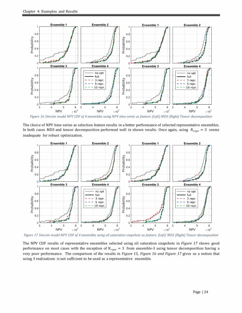
Chapter 4: Examples and Results
Figure 16 Simsim model NPV CDF of 4 ensembles using NPV time series as feature. (Left) MDS (Right) Tensor decomposition
The choice of NPV time series as selection feature results in a better performance of selected representative ensembles. In both cases MDS and tensor decomposition performed well in shown results. Once again, using 𝑁𝑁𝑟𝑟𝑟𝑟𝑟𝑟𝑟𝑟 = 3 seems inadequate for robust optimization.
Figure 17 Simsim model NPV CDF of 4 ensembles using oil saturation snapshots as feature. (Left) MDS (Right) Tensor decomposition
The NPV CDF results of representative ensembles selected using oil saturation snapshots in Figure 17 shows good performance on most cases with the exception of 𝑁𝑁𝑟𝑟𝑟𝑟𝑟𝑟𝑟𝑟 = 3 from ensemble-3 using tensor decomposition having a very poor performance. The comparison of the results in Figure 15, Figure 16 and Figure 17 gives us a notion that using 3 realizations is not sufficient to be used as a representative ensemble.
Page | 24

Chapter 4: Examples and Results
Figure 18 Simsim model NPV CDF of 4 ensembles using (Left) random selection (Right) oil saturation snapshots with SOM
Figure 19 Mean NPV comparison of MDS and tensor decomposition with four ensembles in Simsim model
Figure 18 (left) shows the performance of randomly selected representative ensembles, making clear that random selection is not a good method of choosing representative realizations. However, the results give an important insight to this example used. Firstly, 𝑁𝑁𝑟𝑟𝑟𝑟𝑟𝑟𝑟𝑟 = 10 (i.e., 20% of the full ensemble) seems to be enough representing the full ensemble. Secondly, some ensembles are easier to represent (ensemble-2) than others. Thus, the quantification of performance should have at least more than one example ensemble. Figure 18 (right) is the result from using SOM and
Page | 25

Chapter 4: Examples and Results
oil saturation snapshots for selecting representative models. The performance appears to be on par with the clustering methods.
Figure 19 gives the overall performance on the results presented in in Figure 15, Figure 16 and Figure 17. The mean NPV of ensemble is a good measure for performance since it is also the robust optimization’s objective function. The black bar designates optimized mean NPV for the full ensemble and it is rather clear that 𝑁𝑁𝑟𝑟𝑟𝑟𝑟𝑟𝑟𝑟 = 3 is insufficient as a good representative ensemble. We also notice that NPV time series and oil saturation snapshots are better features for representative selection.
Channel Model
Figure 20 Channel model NPV CDF of 4 ensembles using permeability as feature. (Left) MDS (Right) Tensor decomposition
Figure 21 Channel model NPV CDF of 4 ensembles using NPV time series as feature. (Left) MDS (Right) Tensor decomposition
The results of channel model illustrated in Figure 20 using permeability as feature shows similar performance for MDS and tensor decomposition. All representative ensembles performed very well in all the ensembles shown. However, upon further analysis on more results in Appendix A revealed that 𝑁𝑁𝑟𝑟𝑟𝑟𝑟𝑟𝑟𝑟 = 3 still is insufficient and performed poorly
Page | 26
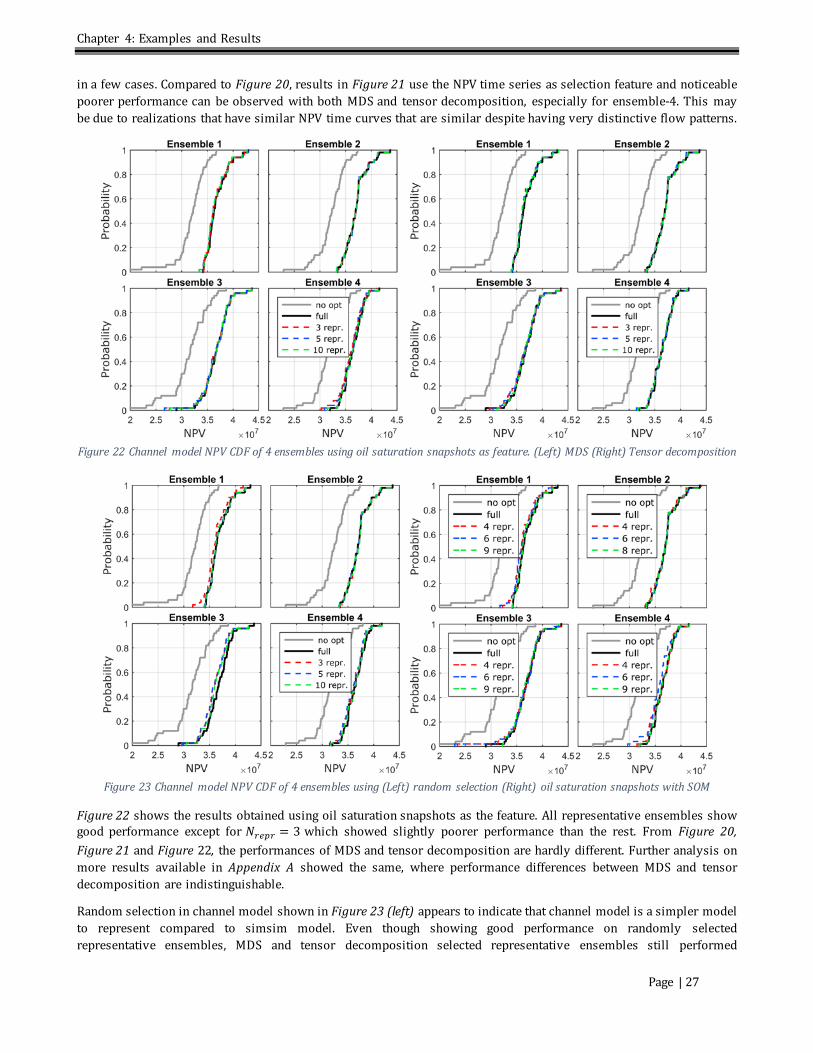
Chapter 4: Examples and Results
in a few cases. Compared to Figure 20, results in Figure 21 use the NPV time series as selection feature and noticeable poorer performance can be observed with both MDS and tensor decomposition, especially for ensemble-4. This may be due to realizations that have similar NPV time curves that are similar despite having very distinctive flow patterns.
Figure 22 Channel model NPV CDF of 4 ensembles using oil saturation snapshots as feature. (Left) MDS (Right) Tensor decomposition
Figure 23 Channel model NPV CDF of 4 ensembles using (Left) random selection (Right) oil saturation snapshots with SOM
Figure 22 shows the results obtained using oil saturation snapshots as the feature. All representative ensembles show good performance except for 𝑁𝑁𝑟𝑟𝑟𝑟𝑟𝑟𝑟𝑟 = 3 which showed slightly poorer performance than the rest. From Figure 20, Figure 21 and Figure 22, the performances of MDS and tensor decomposition are hardly different. Further analysis on more results available in Appendix A showed the same, where performance differences between MDS and tensor decomposition are indistinguishable.
Random selection in channel model shown in Figure 23 (left) appears to indicate that channel model is a simpler model to represent compared to simsim model. Even though showing good performance on randomly selected representative ensembles, MDS and tensor decomposition selected representative ensembles still performed
Page | 27

Chapter 4: Examples and Results
noticeably better. Figure 23 (right) shows that SOM is able to be used as an alternative to the presented selection methods. However results with SOM performs noticeably poorer than the main representative selection method.
Figure 24 NPV comparison of MDS and Tensor with four ensembles in Channel model
Figure 24 provides the comparison of mean NPV in Figure 20, Figure 21 and Figure 22. Once again, 𝑁𝑁𝑟𝑟𝑟𝑟𝑟𝑟𝑟𝑟 = 3 have lower performance than 𝑁𝑁𝑟𝑟𝑟𝑟𝑟𝑟𝑟𝑟 = 5 and 𝑁𝑁𝑟𝑟𝑟𝑟𝑟𝑟𝑟𝑟 = 10 in almost all ensembles. The performances of MDS and tensor decomposition are very similar for the channel model. However, the feature using NPV time series showed a poorer performance, especially for ensemble-4. From the analysis of the results, representative ensembles are thought to be applicable in robust optimization at least in a simple 2D model.
4.2.3 3D Model Egg Model The same workflow of using representative workflow is implemented in Egg Model robust optimization. Figure 25 indicates the final NPV CDF of Egg Model using ensembles of 5, 10 and 20 representative models for robust optimization. The results using representative ensembles are very promising with a few performing even better than the full ensemble. This may be due to a discovered problem in robust optimization carried out using AD-GPRS where, during robust optimization, a few realizations yield gradients that are orders of magnitude higher than the other realizations. Thus, resulting in an inferior robust optimization that is not optimized evenly for all realizations. This is reflected in the full(100) ensemble NPV curve which is lower than full(90) NPV curve where 10 identified realizations with unusually high gradient hae been removed from the ensemble. The problem remains unresolved at the time of writing.
The results showed that having 𝑁𝑁𝑟𝑟𝑟𝑟𝑟𝑟𝑟𝑟 = 5 is sufficient for a good representative ensemble. In representative selection using oil saturation snapshots for both MDS and tensor decomposition, we observe poor performing representative ensemble of 10 and 20 which may be due to the selection of realizations that have unusually high gradient. The results
Page | 28

Chapter 4: Examples and Results
also showed that permeability may be better selection feature in this case. However this may be due to the fact that the Egg model does not have other parameters that will dictates flow pattern.
Figure 25 Egg Model robust optimization results.
4.3 History Matching Results History matching is performed using field production rates of oil and water, the rates is studied to analyze the performance of the representative ensemble. AD-GPRS is used to perform history matching and because AD-GPRS only provide gradients for permeability, the history matching is done by updating the permeability parameters for the reservoir models.
4.3.1 2D Model Simsim Model
Channel Model
Figure 26 Permeability results of history matching using MDS. (Top) Simsim Model (Bottom) Channel Model
Page | 29

Chapter 4: Examples and Results
The porosity of 2D model is modified to be homogeneous as history matching is carried out on permeability only. History matching is performed on the measured water and oil field production for 2D models. The observation error is expressed in terms of standard deviation, 𝜎𝜎𝑟𝑟𝑟𝑟𝑜𝑜𝑝𝑝_𝑟𝑟𝑟𝑟𝑖𝑖𝑟𝑟𝑜𝑜 = 5 m3/day of the production rates measurement. Figure 26 depicts the effect of changes in permeability field in history matching using full ensemble and representative ensembles. For simsim model, representative ensembles has noticeably bigger changes compared to full ensemble.
Simsim Model One of the simplest and illustrative ways to determine the performance of representative ensemble to full ensemble is by visual inspection on field’s production profile of oil and water. The history matching time is arbitrarily selected at 1,500 days to standardize the comparison. Note that history matching is implemented strictly on the production rates measured at 1,500 days (yellow dots) and not the historical data until 1,500 days.
Figure 27 Simsim Model field production data of representative ensemble using all oil saturation snapshots at time 1,500 days. Red is
oil and blue is water. (Left) The priori (Right) The posterior
At first glance, it is clear that the representative ensemble performs well in representing the full ensemble. The dotted line (blurred) depicts the full ensemble and the dashed line portrays the representative ensemble whereas the solid line is the truth realization. By comparing the dotted and dashed line, we noticed the representative ensemble is able to cover the spread of uncertainty in full ensemble. Although comparatively less scattered, the posterior of representative ensemble still has an acceptable spread.
Figure 27 also allows the study on the performance of using two different methods of projection mainly MDS and tensor decomposition, and the number of representative realizations needed. By visual inspection, 𝑁𝑁𝑟𝑟𝑟𝑟𝑟𝑟𝑟𝑟 = 10 have better representation of full ensemble’s uncertainty over 𝑁𝑁𝑟𝑟𝑟𝑟𝑟𝑟𝑟𝑟 = 5 . The comparison of MDS and tensor decomposition shows a little advantage in using MDS as the selected realizations have a better representation of the full ensemble. Although it is inconclusive from Figure 27, further analysis on more data available in Appendix A has showed similar interpretation that MDS performs slightly better.
Figure 28 is to study the effect of history matching at various times. Generally we notice again the representative ensemble performs satisfactory at all control interval time. Note that the representative selection is done considering all the snapshots of oil saturation until end of simulation time, which means that the same representative realizations have been selected for all the plots. One noticeable characteristic concerning the history matching time is a considerably poorer match at t = 450 days and t = 600 days, which is the onset of water breakthrough. The reason behind this may be due to the fact that history matching is done using the field production data rather than individual well production data. The contrast is that at the onset of water breakthrough in field production data resulted in more solutions as water breakthrough in specific well is not known as we are history matching on field production data.
Page | 30

Chapter 4: Examples and Results
Figure 28 Simsim Model field production data of posterior of 10 representative realizations using MDS and all oil saturation
snapshots at various history matching time. Red is oil and blue is water
Figure 29 Simsim Model field production data of posterior of 10 representative realizations using MDS and oil saturation snapshots
up to specified history matching time. Red is oil and blue is water
Page | 31

Chapter 4: Examples and Results
Figure 29 differs from Figure 28: here the selection of representative realizations in Figure 29 is based on oil saturation snapshots up until the history matching time making the feature data sparser and at earlier t < 1,200 days the feature data may not be sufficient for a good representative model selection. The first apparent observation by comparing Figure 28 and Figure 29 is that history matching at earlier times performs worse in Figure 29. This is most likely due to the fact that the saturation snapshots taken at earlier times have insufficient data to differentiate between realizations effectively. As the time to history match increases, the representative model selection shows improvement and even shares the same realizations as in Figure 28.
Figure 30 Simsim Model NPV comparison of 10 representative realizations using MDS. Repr prior all and repr post all are selected
using all oil saturation snapshots whereas repr prior and repr post are selected using oil saturation snapshots up to the history matching time. (Left) The prior NPV CDF plot. (Right) The posterior NPV CDF plot.
Another way to determine performance is to analyze the NPV of the ensemble. In essence the representative ensemble’s NPV distribution should favorably have a good representation of full ensemble’s NPV distribution. For this comparison we study the prior and posterior NPV CDF plot of the ensembles in Figure 30. Note that no optimization is carried out on the ensemble thus shifting of the NPV CDF curves does not reflect performance. Also for that reason, the full ensemble’s curve will be the reference and a closer match of representative ensemble on full ensemble’s curve will be interpreted as good representation.
In Figure 30(left), prior representative all have a good representation of the full ensemble’s NPV CDF plot however repr prior shows a weaker representation. In Figure 30(right), both representative ensembles have very similar curves to each other. However, they do not match to the curve of full ensemble. Almost all posterior NPV CDF shows smaller spread compared to the prior except for history matching done in the later time of which the spread of NPV grows. One possibility is that due to having higher water production rate and much lower oil production rate at the later part of the history matching time, which will greatly affect the NPV as it relies heavily on oil price and water injection/production cost.
Channel Model In channel model, similar results as presented previously are shown in this section. Figure 31 is similar to Figure 27 where the comparison of prior and posterior production profiles is done. Again, the representative ensembles provide acceptable representation of the full ensemble’s uncertainty in both cases. The posterior in Figure 31(right) shows noticeable reduction in spread of uncertainty especially on the water production rate. However the reduction in
Page | 32

Chapter 4: Examples and Results
spread is marginal. The difference between the performance of MDS and tensor decomposition is much less noticeable compared to Figure 27. However, 𝑁𝑁𝑟𝑟𝑟𝑟𝑟𝑟𝑟𝑟 = 10 seems to have a better representation than 𝑁𝑁𝑟𝑟𝑟𝑟𝑟𝑟𝑟𝑟 = 5.
Figure 31 Channel Model field production data of representative ensemble using all oil saturation snapshots at time 1,500 days. Red
is oil and blue is water. (Left) The prior (Right) The posterior
Figure 32 Channel Model field production data of posterior of 10 representative realizations using MDS and all oil saturation
snapshots at various history matching time. Red is oil and blue is water
Figure 32 shows that for channel model, choosing the history matching at different time does not have any real impact on the history matched results. It could be due to the fact that the truth is an outlier realization. Meaning that more
Page | 33

Chapter 4: Examples and Results
significant model updates are needed and the regularization term in history matching is preventing larger changes to preserve initial model channel location.
Figure 33 Channel Model field production data of posterior of 10 representative realizations using MDS and oil saturation snapshots
up to specified history matching time. Red is oil and blue is water
Figure 34 Channel Model NPV comparison of 10 representative realizations using MDS. Repr prior all and repr post all are selected
using all oil saturation snapshots whereas repr prior and repr post are selected using oil saturation snapshots up to the history matching time. (Left) The prior NPV CDF plot. (Right) The posterior NPV CDF plot.
Page | 34

Chapter 4: Examples and Results
Figure 33 shows the selection based on oil saturation of snapshot up to the history matching time. A comparison between Figure 32 and Figure 33 and suggests that selecting representative realizations based on all oil saturation snapshots is more advantageous over only based on oil saturation snapshot up to certain history matching time. Figure 34 compares the representative realizations selection based on NPV CDF plots. In terms of NPV, both selection based on different history matching time and all saturation snapshots shows similar result and they conform well to the full ensemble NPV CDF curve.
In all, the representative ensembles prove to be sufficient to replace full ensemble in history matching without compromising uncertainty quantification too much. The prior and posterior of the representative ensemble still cover adequate spread in uncertainty when compared to full ensemble’s uncertainty spread although understandably less.
4.3.2 3D Model Egg Model History matching of Egg Model is performed using the field oil and water production rates and each injectors’ pressure. The observation error is expressed in terms of production rates standard deviation, 𝜎𝜎𝑟𝑟𝑟𝑟𝑜𝑜𝑝𝑝 _𝑟𝑟𝑟𝑟𝑖𝑖𝑟𝑟𝑜𝑜 = 5 m3/day and injectors’ pressure standard deviation, 𝜎𝜎𝑖𝑖𝑛𝑛𝑖𝑖_𝑟𝑟𝑟𝑟𝑟𝑟𝑜𝑜𝑜𝑜𝑓𝑓𝑟𝑟𝑟𝑟 = 10 bar of the measurement. For Egg Model, the time of history matching is arbitrarily chosen to be at 1,800 days.
MDS
Tensor Decomposition
Figure 35 Examples of history matched layer 4 of Egg Model permeability field using (Top) MDS (Bottom) Tensor decomposition.
Figure 35 shows the effect of history matching on the permeability field. Similar to what was observed in 2D model, the changes in permeability field of representative ensemble is bigger than of full ensemble. The results comparison of Egg Model are based on the field water and oil production data similar to the results of 2D models. Since the history matching of the Egg Model is carried out using the injectors’ pressure as well, looking at the pressure profile of each injectors can shed some insight on the performance of the representative ensembles compared to the full ensemble.
Page | 35

Chapter 4: Examples and Results
Figure 36 Egg Model water (blue) and oil (red) production rates. Representative ensembles selected using MDS.
Figure 37 Egg Model injector rates of representative ensembles using MDS as projection method. (Left) Prior (Right) Posterior
The first comparison with full ensemble is the field water and oil production illustrated in Figure 36 and injectors pressure Figure 37 where MDS is used to choose the representative ensembles. Both figures show similar results where a slight reduction in the spread of both rates are noticeable in the posterior results. In Figure 36, a few realizations of the full ensemble have showed larger spread in the posterior result which may due to improper changes in permeability field during history matching. During the history matching simulation, a few realizations have been noticed to require far greater time for simulation which suggested a poor update on the realizations’ permeability
Page | 36

Chapter 4: Examples and Results
field. This problem was not encountered in the representative ensembles simulations. Figure 37 depicts the injectors’ pressure of representative ensembles against the full ensemble. The representative ensembles are able to have similar outline as the full ensemble although understandably less. 𝑁𝑁𝑟𝑟𝑟𝑟𝑟𝑟𝑟𝑟 = 10 showed a rather deficient coverage of the uncertainty and is considered rather insufficient to represent the full ensemble.
Figure 38 Egg Model water (blue) and oil (red) production rates. Representative ensembles selected using tensor decomposition.
Figure 39 Egg Model injector rates of representative ensembles using tensor decomposition as projection method. (Left) Prior (Right)
Posterior
Page | 37

Chapter 4: Examples and Results
Similar to Figure 36 and Figure 37, Figure 38 and Figure 39 compare the performance of representative ensembles using tensor decomposition. Figure 38 showed a good representation on the field production rates. Tensor decomposition provides a larger spread in pressure profile when comparing Figure 39 to Figure 37 of using MDS. In spite of that, it is hard to distinguish the performance difference between the two projection methods with visual inspection. However, it is rather clear that 𝑁𝑁𝑟𝑟𝑟𝑟𝑟𝑟𝑟𝑟 = 10 is not able to have a good representation from the injectors’ pressure profile. This observation is noticeable in both projection methods used where, in a few cases, have highly deviated pressure profile. From the figures, the representative ensembles provide a relatively good matches to the curve and spread of full ensemble. Although, it is clear that 𝑁𝑁𝑟𝑟𝑟𝑟𝑟𝑟𝑟𝑟 = 20 represents the uncertainty spread much better than using 𝑁𝑁𝑟𝑟𝑟𝑟𝑟𝑟𝑟𝑟 = 10 .
Figure 40 Normalized sum of square error at 1,800 days of field oil and water production rates to the truth.
Figure 40 depicts the normalized sum of squared error (SSE) of the water and oil production rates compared at 1,800 days. SSE provides an indication to the spread of the uncertainty to some extent. In our application case, closer match to full ensemble’s normalized SSE value can be viewed as the reference since uncertainty covered is as important as accuracy. Both water and oil production rates’ SSE are very similar, this may be due to the same weightage in history matching. A large increase in the posterior SSE of full ensemble’s water production rates is most probably due to the poorly updated realizations as mentioned previously. Generally, there should be reduction in the normalized posterior SSE values which are observed in representative ensembles using MDS but not tensor decomposition. With considering 𝜎𝜎𝑟𝑟𝑟𝑟𝑜𝑜𝑝𝑝_𝑟𝑟𝑟𝑟𝑖𝑖𝑟𝑟𝑜𝑜 = 5 m3/day meaning the SSE may have an acceptable deviation of 25 m3/day, thus all the representative ensembles are within an acceptable range compared to the full ensemble.
Page | 38

Chapter 4: Examples and Results
Figure 41 Egg Model history matching prior and posterior final NPV CDF using full ensemble and representative ensemble selected
using MDS and tensor decomposition.
Figure 41 depicts the final NPV CDF of prior and posterior in order to compare both MDS and tensor decomposition selected representative ensembles. The truth realization has a final NPV of 16 million and all the posterior NPV CDF have a noticeable shift towards the truth’s NPV which indicate history matching is performing effectively. In terms of number of representative realizations, both 𝑁𝑁𝑟𝑟𝑟𝑟𝑟𝑟𝑟𝑟 = 10and 𝑁𝑁𝑟𝑟𝑟𝑟𝑟𝑟𝑟𝑟 = 20 have similar curve thus does not offer clear performance difference among them. It is clear from Figure 41 that tensor decomposition representative ensembles have better match with the full ensemble’s NPV CDF compared to MDS selected representative ensembles especially in the posterior results.
Page | 39

Chapter 5: Discussion
5. Discussion The discussion is separated into a few category of relevance. Firstly, the summary of the methodology, findings and possible improvements of this thesis are examined.
1. Features have been identified as a critical component in the selection of representative models. Therefore, various features were compared on simple 2D models and we have chosen to focus on permeability, NPV time series and oil saturation snapshots. From the results, permeability and oil saturation snapshots were found to be better. The reason NPV time series was not performing up to par is thought to be due to NPV relying on economic factors thus limiting the ability of differentiating between realizations. Although permeability was a good feature in our case, it is not recommended for models that contain other properties that can influence the flow characteristic of the models.
2. Considering projection or dimensionality reduction is important to the methodology, where two principally different techniques were implemented. However, we have found little to no noticeable difference in the effectiveness of tensor decomposition compared to MDS as a projection technique for clustering. In tensor decomposition, the cutoff criteria which used 95% of the cumulative energy content for projection dimension remained an unstudied problem. Nevertheless, case models used are admittedly rather simple where more complex model may show different results and may give better insight on the performance of MDS compared to tensor decomposition.
3. Although features are very important for the effectiveness of representative selection, MDS projection relies heavily on the pairwise distance between realizations. Therefore, the type of distance measures may have notable impact on the projected data. This thesis only applied Euclidean distance in using MDS and the effect of distance measure may be pursued in future works.
4. K-means clustering partitions data into groups with unique centroids which is the ideal representative point of each groups. The selected representative models have to be compromised to the one closest to each centroids thus introducing imperfection to the representative ensembles. This may explain why some representative ensemble has substandard performance in a few cases especially evident with 𝑁𝑁𝑟𝑟𝑟𝑟𝑟𝑟𝑟𝑟 = 3 . Although not tested, the distance of selected realizations to the centroid may be a criteria for reselection of representative realizations.
5. SOM was introduced where the clustering is solely based on grouping by competition, consequently similar realizations will be grouped together. However, the clustering technique with SOM presented here is an exploratory attempt to provide an alternative to K-means clustering. Further studies are required for many parameters such as number of training iteration, stopping criteria, the competition function and the effect of amplitude of neighborhood to determine their appropriate value. In spite of that, preliminary use of SOM resulted in comparable performance with K-means clustering with using MDS or tensor decomposition as projection method.
6. Since the goal was to discover the bare minimum representative models needed to represent an ensemble, the amount of realizations has to be drastically reduced. Thus, in order to preserve the full ensemble statistically, weighting is needed for each representative models. We have investigated the importance of weight from simulation runs and concluded that weighting is essential and thus included in the methodology. Many types of weighting scheme may be applied. Therefore, there are rooms to improve the representative ensembles’ performance by identifying a more suitable weighting scheme such as one that takes the distance of realizations to centroid into account.
Next, the results and recommendation for future works that may improve this methodology are discussed.
1. The goal of this thesis was to accelerate robust optimization and history matching by using far less realizations than the original ensemble. Based on the results obtained for our case studies, representative ensembles can undoubtedly be used to accelerate robust optimization workflows. The minimum representative realizations seems to be around 5 to 10 reservoir models, although more studies should be carried out to ascertain this statement.
Page | 40

Chapter 5: Discussion
2. The performance of using representative ensembles in history matching was not as well defined as in robust optimization although it was still able to capture most of the quantified uncertainties. Compared to full ensemble, the representative ensembles still cover big portion of the uncertainty spread. In 2D models, 𝑁𝑁𝑟𝑟𝑟𝑟𝑟𝑟𝑟𝑟 = 10 outperforms 𝑁𝑁𝑟𝑟𝑟𝑟𝑟𝑟𝑟𝑟 = 5 whereas in Egg Model, 𝑁𝑁𝑟𝑟𝑟𝑟𝑟𝑟𝑟𝑟 = 20 performs better than 𝑁𝑁𝑟𝑟𝑟𝑟𝑟𝑟𝑟𝑟 = 10 . This may indicate that the minimum number of realizations required for history matching is related to the percentage representation of the full ensemble contrary to robust optimization. Understandably, an ensemble should provide UQ for the reservoir and naturally having less realizations in representative ensemble reduces the ability for UQ. It is important to note that each representative realizations has its own weightage and visual inspection on the spread was unable to take that into account.
3. The results have shown that proposed methodology can be implemented in robust optimization and history matching. Therefore, using this method should be applicable to CLRM without the need of extensive modifications to the workflow, provided that adjoint-based optimization is available (Barros et al., 2016b). However, there is more work to be done if we wish to apply this methodology in ensemble-based optimization.
4. The speedup obtained by using representative ensembles can be further increased with the incorporation of ROM techniques such as multiscale method. If proved attainable, this is a step in the right direction to realize the VOI workflow that has been unfeasible in terms of computational cost until now.
The validation of the results has faced many challenges, those challenges are presented in the following section.
1. Although not included in this report, various analyses were carried out to assure good selection of realizations before further optimizations, but the lack of samples made most statistical tests inadequate. Stage 1 validation (Figure 8) of the selected representative models remains a huge challenge. The main reason is that representative ensemble is a subset of the full ensemble and have much less realizations than the full ensemble. Therefore, classical statistical tests such as variance explained are not suitable as a measure because the results in variance explained are always lower than the full ensemble. The mean of ensembles has been tested but it does not reflect the quality of selected representative models when compared with stage 2 results. The covariance matrices of representative ensembles are of much lower rank compared to full ensemble. Thus, covariance suffers from the same problem as variance as well as the entropy of SVD of representative when compared to full ensemble. KS-test performed in stage 1 validation also proved ineffective. Although applicable to provide a quantitative measurement of fit to NPV of full ensemble, robust optimization changes the final NPV where conformity to the initial unoptimized NPV is thus meaningless.
2. Clustering validation provides a measure on how well the clustering algorithm performs based on criterion function. However, it does not provide a measure on how well the original dataset is clustered based on patterns of data. Jain and Dubes (1988) stated that “the validation of clustering structures is the most difficult and frustrating part of cluster analysis. Without a strong effort in this direction, cluster analysis will remain a black art accessible only to those true believers who have experience and great courage.”
Lastly, we comment on the general understandings of the topic address in this thesis which are predominantly conjectural.
1. Ideally, there is only one strategy for robust optimization which maximizes the objective function while being constrained to all realizations. Intuitively, representative models can ‘pull’ the robust optimization towards that ideal strategy. However, ensembles that have less than 5 representative models proved to be difficult as having one more or one less realization affects the ability of the representative ensemble to ‘gravitate’ in the right direction. Example shown in Insuasty et al. (2015) which uses 50 realizations out of 1000 realizations should be possible to be reduced further to 10 or even less realizations and still provide a comparable optimal production strategy.
2. Currently, the comparison of history matching performance is carried out trying to match the spread of the full ensemble in terms of production rates or the NPV CDF curve or injectors’ pressure (only for Egg Model). However, it is not clear whether this approach is considered better because, alternatively, it may also be desirable for the representative ensemble to have history matched results closer to the truth. Without a quantitative clarification on this matter, the performance of representative ensembles in history matching remains unquantifiable.
Page | 41

Chapter 5: Discussion
3. In the channel model example for history matching, all the posterior results are very similar. The reasoning was that the regularization term is preventing further changes in the permeability field. As the author’s personal opinion, the geological accuracy in the model is somewhat overrated by having the conventional regularization term in history matching. If the observed data are clearly showing a very different measurements than expected, it may simply mean that the model is very different from the truth, thus, there is very little incentive in preserving geological accuracy in the first place. This thinking is also recounted by Kahrobaei (2016) using a simple 2D model. By removing the regularization term, his history matching procedure was able to reveal hidden geological features (e.g., barrier and high permeable streak) present in the true permeability field.
4. The method for selection for representative models presented in this thesis uses simulated feature data. In real reservoir management, measured data could be incorporated as a feature in choosing the representative models which are more likely to reflect the real reservoir. Therefore, a reselection of representative realizations may be beneficial at the first history matching interval.
Page | 42

Chapter 6: Conclusion
6. Conclusion The goal of the thesis was to accelerate workflow of robust optimization and history matching by using representative models to reduce the total computational cost. The thesis found that representative ensemble is highly effective in robust optimization. Having 5 or more representative models are sufficient in both 2D and 3D models tested to obtain a comparable optimal strategy to using a full ensemble. Nevertheless, the case studies we considered here are not as complex as real field models. Still, the results in robust optimization are very promising and should be tested in real field applications.
In history matching, presented results suggest that using 20 realizations (20% of the full ensemble) allows to quantify most of the uncertainties while achieving history matched models that are comparable to those obtained considering the full ensemble. Even so, using representative ensembles in history matching remains an open debate as there is a marginal decrease in the quality of UQ compared to using the full ensemble. Consequently, the choice of 𝑁𝑁𝑟𝑟𝑟𝑟𝑟𝑟𝑟𝑟 in history matching should be a compromise between the amount of acceleration required and the importance of UQ to the application purpose.
In terms of computational cost, our case studies showed that representative ensembles are capable of significantly reducing the number of simulations in robust optimization and history matching. The speedup is directly proportional to the percentage reduction in representative realizations used. When combining both robust optimization and history matching in CLRM, utilizing only 10% of full ensemble in one of the two processes is estimated to yield a speedup of two times assuming both have similar computational cost. Furthermore, by using 10% of full ensemble in both processes, an acceleration of one order of magnitude will be attainable in the CLRM workflow.
Page | 43

References Aggarwal, C. C., Wolf, J. L., Yu, P. S., Procopiuc, C., & Park, J. S. (1999, June). Fast algorithms for projected clustering. In ACM SIGMoD Record (Vol. 28, No. 2, pp. 61-72). ACM.
Anderberg, M. R. (2014). Cluster analysis for applications: probability and mathematical statistics: a series of monographs and textbooks (Vol. 19). Academic press.
Arabie, P. and Hubert, L.J. (1996). An overview of combinatorial data analysis. Clustering and Classification, pp. 5-63. World Scientific Pub., New Jersey.
Arthur, D., & Vassilvitskii, S. (2007, January). k-means++: The advantages of careful seeding. In Proceedings of the eighteenth annual ACM-SIAM symposium on discrete algorithms (pp. 1027-1035). Society for Industrial and Applied Mathematics.
Barros, E.G.D., Van den Hof, P.M.J. and Jansen, J.D. (2016a). Value of information in closed-loop reservoir management. Computational Geosciences 20(3), 737-749. DOI: 10.1007/s10596-015-9509-4.
Barros, E.G.D., Yap, F.K., Insuasty Moreno, E.G., Van den Hof, P.M.J. and Jansen, J.D. (2016b). Clustering Techniques for Value-of-Information Assessment in Closed-Loop Reservoir Management. Proc. 15th European Conference on Mathematics in Oil Recovery (ECMOR XV), Amsterdam, The Netherlands, 29 August - 1 September.
Berchtold, S., Böhm, C., Keim, D. A., & Kriegel, H. P. (1997, May). A cost model for nearest neighbor search in high-dimensional data space. In Proceedings of the sixteenth ACM SIGACT-SIGMOD-SIGART symposium on Principles of database systems (pp. 78-86). ACM.
Borg, I., Groenen, P. (1997). Modern multidimensional scaling: theory and applications. Springer, New York, 614 p.
Brouwer, D. R., & Jansen, J. D. (2002, January). Dynamic optimization of water flooding with smart wells using optimal control theory. In European Petroleum Conference. Society of Petroleum Engineers.
Cabanes, G., & Bennani, Y. (2010). Learning the number of clusters in Self Organizing Map. INTECH Open Access Publisher.
Chen, C., Li, G., & Reynolds, A. (2012). Robust constrained optimization of short-and long-term net present value for closed-loop reservoir management. SPE Journal, 17(03), 849-864.
Deboeck, G.J., (1998). Financial applications of self-organizing maps. Electronic Newsletter American Heuristics, Inc., 7p.
Dubes, R. C. (1993, December). Cluster analysis and related issues. In Handbook of pattern recognition.
Hewson, C.W. (2015) Reduced-Order Modelling for Production Optimisation. Published master’s thesis, Delft University of Technology, Delft, the Netherlands.
Insuasty, E., Van den Hof, P. M. J., Weiland, S., & Jansen, J. D. (2015a, February). Spatial-temporal tensor decompositions for characterizing control-relevant flow profiles in reservoir models. In SPE Reservoir Simulation Symposium. Society of Petroleum Engineers.
Insuasty, E., Van den Hof, P. M., Weiland, S., & Jansen, J. D. (2015b). Tensor-based reduced order modeling in reservoir engineering: An application to production optimization. IFAC-PapersOnLine, 48(6), 254-259.
J. He, “Reduced-Order Modeling For Oil-Water and Compositional Systems, with Applications to Data Assimilation and Production Optimization,” Stanford, USA, October 2013.
Jacquard, P. and Jain, C. (1965). Permeability Distribution from Field Pressure Data, Soc. Pet. Eng. Journal, 281-294.
Jain, A. K., & Dubes, R. C. (1988). Algorithms for clustering data. Prentice-Hall, Inc.
Jain, A. K., Murty, M. N., & Flynn, P. J. (1999). Data clustering: a review. ACM computing surveys (CSUR), 31(3), 264-323.
Page | 44

Jansen, J. D., Bosgra, O. H., & Van den Hof, P. M. (2008). Model-based control of multiphase flow in subsurface oil reservoirs. Journal of Process Control, 18(9), 846-855.
Jansen, J. D., Brouwer, R., & Douma, S. G. (2009, January). Closed loop reservoir management. In SPE Reservoir Simulation Symposium. Society of Petroleum Engineers.
Jansen, J. D., Fonseca, R. M., Kahrobaei, S., Siraj, M. M., Van Essen, G. M., & Van den Hof, P. M. J. (2014). The egg model–a geological ensemble for reservoir simulation. Geoscience Data Journal, 1(2), 192-195.
Jardine, N., & Sibson, R. (1971). Mathematical taxonomy. London etc.: John Wiley.
Kaleta, M. P., Hanea, R. G., Heemink, A. W., & Jansen, J. D. (2011). Model-reduced gradient-based history matching. Computational Geosciences, 15(1), 135-153.
Kahrobaei, S.S. (2016). Identification of Flow-Relevant Structural Features in History Matching. Published master’s thesis, Delft University of Technology, Delft, the Netherlands. DOI:10.4233/uuid:3bcb57b0-379c-4a13-a297-ffa9e9ce0910
Kaski, S. (1997). Data exploration using self-organizing maps. In Acta Polytechnica Scandinavica: Mathematics, computing and management in engineering series no. 82.
Kiang, M. Y. (2001). Extending the Kohonen self-organizing map networks for clustering analysis. Computational Statistics & Data Analysis, 38(2), 161-180.
Klose, C. D. (2006). Self-organizing maps for geoscientific data analysis: geological interpretation of multidimensional geophysical data. Computational Geosciences, 10(3), 265-277.
Kohonen Network - Background Information. (2012). Retrieved August 09, 2016, from http://www.lohninger.com/helpcsuite/kohonen_network_-_background_information.htm
Kohonen, T. (1990). The self-organizing map. Proceedings of the IEEE,78(9), 1464-1480.
Kohonen, T., Oja, E., Simula, O., Visa, A., & Kangas, J. (1996). Engineering applications of the self-organizing map. Proceedings of the IEEE, 84(10), 1358-1384.
Krogstad, S., Hauge, V. L., & Gulbransen, A. (2011). Adjoint multiscale mixed finite elements. SPE Journal, 16(01), 162-171.
Kruger, W. D. (1961). Determining Areal Permeability Distribution by Calculation. J. Pet. Tech., 691.
Kruskal, J. B. (1964). Nonmetric multidimensional scaling: a numerical method. Psychometrika, 29(2), 115-129.
Lie, K.-A., Krogstad, S., Ligaarden, I.S., Natvig, J.R., Nilsen, H.M. and Skalestad, B. (2012) Open source MATLAB implementation of consistent discretisations on complex grids. Computational Geosciences, 16(2), 297-322.
MacQueen, J. (1967, June). Some methods for classification and analysis of multivariate observations. In Proceedings of the fifth Berkeley symposium on mathematical statistics and probability (Vol. 1, No. 14, pp. 281-297).
Oliver, D. S. and Y. Chen (2011). Recent progress on reservoir history matching: a review. Computational Geosciences 15(1), 185–221
Ouenes, A., Weiss, W., Sultan, A. J., & Anwar, J. (1995, January). Parallel Reservoir Automatic History matching using a network of Workstations and PVM. In SPE Reservoir Simulation Symposium. Society of Petroleum Engineers.
Park, K. and J. Caers (2007). History matching in low-dimensional connectivity-vector space. In EAGE Petroleum Geostatistics.
Parsons, L., Haque, E., & Liu, H. (2004). Subspace clustering for high dimensional data: a review. ACM SIGKDD Explorations Newsletter, 6(1), 90-105.
Penn, B. S. (2005). Using self-organizing maps to visualize high-dimensional data. Computers & Geosciences, 31(5), 531-544.
Page | 45

Salazar, V. M., Schiozer, D. J., & Monticelli, A. J. (1996, January). External Parallelization of Reservoir Simulators Using a Network of Workstations and PVM. In SPE Latin America/Caribbean Petroleum Engineering Conference. Society of Petroleum Engineers.
Sarma, P., Durlofsky, L. J., Aziz, K., & Chen, W. H. (2006). Efficient real-time reservoir management using adjoint-based optimal control and model updating. Computational Geosciences, 10(1), 3-36.
Sarma, P., Chen, W. H., & Xie, J. (2013, February 18). Selecting Representative Models From a Large Set of Models. Society of Petroleum Engineers. doi:10.2118/163671-MS
Scheidt, C. and J. Caers (2009). Representing spatial uncertainty using distances and kernels. Mathematical Geosciences 41 (4), 397–419.
Scheidt, C., J. Caers, et al. (2009). Uncertainty quantification in reservoir performance using distances and kernel methods–application to a west africa deepwater turbidite reservoir. SPE Journal 14 (04), 680–692.
Scheidt, C., J. Caers, Y. Chen, and L. Durlofsky (2011). A multi-resolution workflow to generate high-resolution models constrained to dynamic data. Computational Geosciences 15 (3), 545–563.
Schiozer, D. J. (1999, January). Use of Reservoir simulation, Parallel computing and Optimization techniques to accelerate History Matching and Reservoir management decisions. In Latin American and Caribbean Petroleum Engineering Conference. Society of Petroleum Engineers.
Shepard, D. (1968) A two-dimensional interpolation function for irregularly-spaced data, Proc. 23rd National Conference ACM, ACM, 517-524.
Sneath, P. H., & Sokal, R. R. (1973). Numerical taxonomy. The principles and practice of numerical classification.
Strebelle, S. [2002] Conditional simulation of complex geological structures using multiple-point statistics. Mathematical Geology 34(1) 1–22. DOI: 10.1023/A:1014009426274.
Suzuki, S. and J. Caers (2008). A distance based prior model parameterization for constraining solution of spatial inverse problems. Mathematical Geosciences 40 (4), 445–469.
Suzuki, S., G. Caumon, and J. Caers (2008). Dynamic data integration for structural modeling: model screening approach using a distance-based model parameterization. Computational Geosciences 12 (1), 105–119. DOI: 10.1007/s10596–007–9063–9.
van Essen, G. M., Zandvliet, M. J., Van den Hof, P. M. J., Bosgra, O. H., & Jansen, J. D. (2006, October). Robust optimization of oil reservoir flooding. In 2006 IEEE Conference on Computer Aided Control System Design, 2006 IEEE International Conference on Control Applications, 2006 IEEE International Symposium on Intelligent Control (pp. 699-704). IEEE.
van Essen, G., Zandvliet, M., Van den Hof, P., Bosgra, O., & Jansen, J. D. (2009). Robust waterflooding optimization of multiple geological scenarios. SPE Journal, 14(01), 202-210.
Vesanto, J. (1999). SOM-based data visualization methods. Intelligent data analysis, 3(2), 111-126.
Vesanto, J., & Alhoniemi, E. (2000). Clustering of the self-organizing map. IEEE transactions on neural networks, 11(3), 586-600.
Voskov, D. V., & Zhou, Y. (2012). Technical Description of the AD-GPRS. Department of Energy Resources Engineering. Stanford University
Yasari, E., Pishvaie, M. R., Khorasheh, F., Salahshoor, K., & Kharrat, R. (2013). Application of multi-criterion robust optimization in water-flooding of oil reservoir. Journal of Petroleum Science and Engineering, 109, 1-11.
Zandvliet, M. J., Bosgra, O. H., Jansen, J. D., Van den Hof, P. M. J., & Kraaijevanger, J. F. B. M. (2007). Bang-bang control and singular arcs in reservoir flooding. Journal of Petroleum Science and Engineering, 58(1), 186-200.
Page | 46

Appendix A
Figure 42 Simsim model NPV CDF of 6 additional ensembles using permeability as feature. (Left) MDS (Right) Tensor decomposition
Figure 43 Simsim model NPV CDF of 6 additional ensembles using NPV time series as feature. (Left) MDS (Right) Tensor
decomposition
Page | I
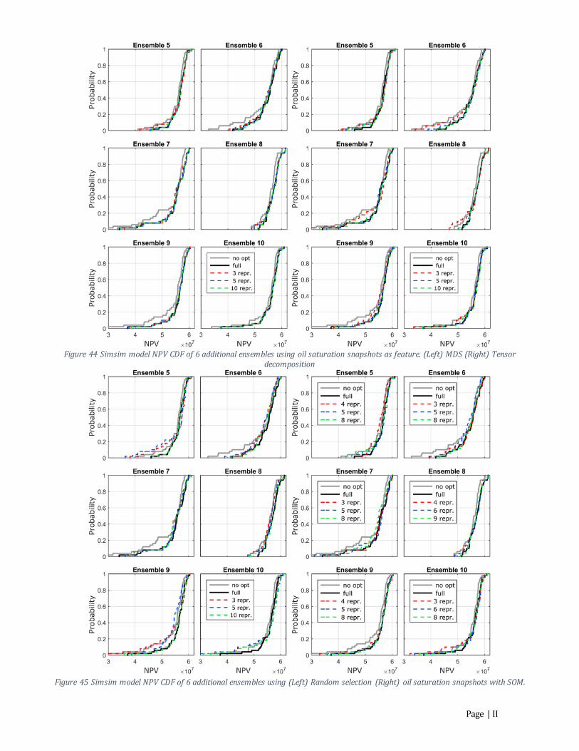
Figure 44 Simsim model NPV CDF of 6 additional ensembles using oil saturation snapshots as feature. (Left) MDS (Right) Tensor
decomposition
Figure 45 Simsim model NPV CDF of 6 additional ensembles using (Left) Random selection (Right) oil saturation snapshots with SOM.
Page | II

Figure 46 Channel model NPV CDF of 6 additional ensembles using permeability as feature. (Left) MDS (Right) Tensor decomposition
Figure 47 Channel model NPV CDF of 6 additional ensembles using NPV time series as feature. (Left) MDS (Right) Tensor
decomposition
Page | III

Figure 48 Channel model NPV CDF of 6 additional ensembles using oil saturation snapshots as feature. (Left) MDS (Right) Tensor
decomposition
Figure 49 Channel model NPV CDF of 6 additional ensembles using (Left) Random selection (Right) oil saturation snapshots with
SOM
Page | IV

Appendix B The Kolmogorov–Smirnov test (KS test) is a nonparametric test of the equality of continuous, one-dimensional probability distributions that can be used to compare a sample with a reference probability distribution (one-sample KS test), or to compare two samples (two-sample KS test). Two-sample KS test is used to test whether two underlying distributions differ significantly. The KS-test has the advantage of making no assumption about the distribution of data. More information on KS test can be found at Chakravart, Laha, and Roy, (1967).
Page | V