Embed Size (px)
Citation preview

FSAN/ELEG815: Statistical Learning
Gonzalo R. ArceDepartment of Electrical and Computer Engineering
University of Delaware
5a: The Linear Model and Optimization
1/50
FSAN/ELEG815
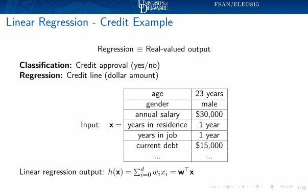
Linear Regression - Credit Example
Regression ≡ Real-valued output
Classification: Credit approval (yes/no)Regression: Credit line (dollar amount)
Input: x =
age 23 yearsgender male
annual salary $30,000years in residence 1 year
years in job 1 yearcurrent debt $15,000
... ...
Linear regression output: h(x) =∑di=0wixi = w>x

2/50
FSAN/ELEG815
Credit Example Again - The data set
Input: x =
age 23 yearsgender male
annual salary $30,000years in residence 1 year
years in job 1 yearcurrent debt $15,000
... ...
Output:
h(x) =d∑i=0
wixi = w>x
Credit officers decide on credit lines:
(x1,y1),(x2,y2), · · · ,(xN ,yN )
yn ∈ R is the credit for customer xn.
Linear regression wants to automate this task, trying to replicate humanexperts decisions.

3/50
FSAN/ELEG815
Linear Regression
Linear regression algorithm is based on minimizing the squared error:
Eout(h) = E[(h(x)−y)2]
where E[·] is taken with respect to P (x,y) that is unknown.Thus, minimize the in-sample error:
Ein(h) = 1N
N∑n=1
(h(xn)−yn)2
Find a hypothesis (w) that achieves a small Ein.
4/50
FSAN/ELEG815
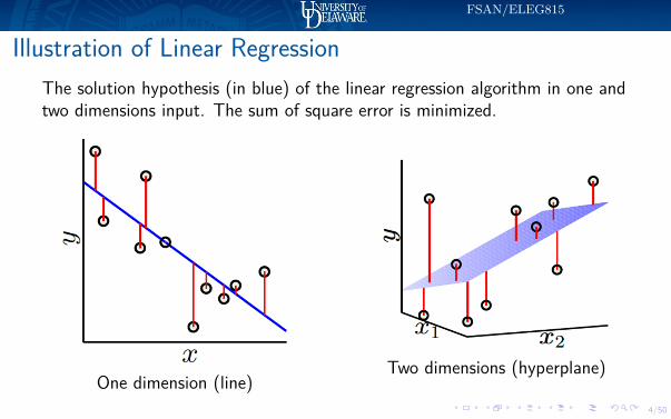
Illustration of Linear RegressionThe solution hypothesis (in blue) of the linear regression algorithm in one andtwo dimensions input. The sum of square error is minimized.
One dimension (line)Two dimensions (hyperplane)
5/50
FSAN/ELEG815
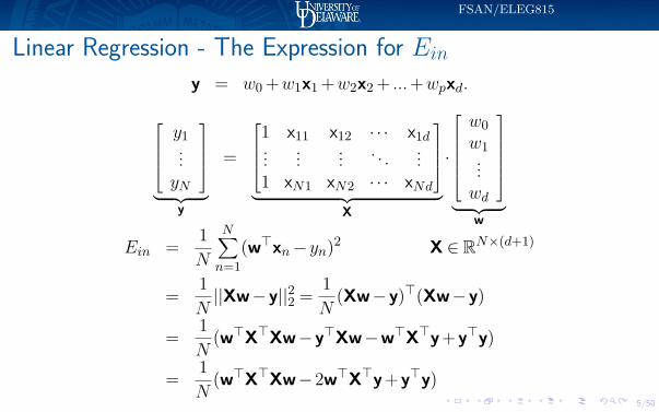
Linear Regression - The Expression for Einy = w0 +w1x1 +w2x2 + ...+wpxd.
y1...yN
︸ ︷︷ ︸
y
=
1 x11 x12 · · · x1d... ... ... . . . ...1 xN1 xN2 · · · xNd
︸ ︷︷ ︸
X
·
w0w1...wd
︸ ︷︷ ︸
w
Ein = 1N
N∑n=1
(w>xn−yn)2 X ∈ RN×(d+1)
= 1N||Xw−y||22 = 1
N(Xw−y)>(Xw−y)
= 1N
(w>X>Xw−y>Xw−w>X>y+y>y)
= 1N
(w>X>Xw−2w>X>y+y>y)

6/50
FSAN/ELEG815
Learning Algorithm - Minimizing Ein
w = arg minw∈Rd
1N||Xw−y||22
= arg minw∈Rd
1N
(w>X>Xw−2w>X>y+y>y)
Observation: The error is a quadratic function of wConsequences: The error is an (d+1)–dimensional bowl–shaped function of wwith a unique minimumResult: The optimal weight vector, w, is determined by differentiating Ein(w)and setting the result to zero
∇wEin(w) = 0
I A closed form solution exists
7/50
FSAN/ELEG815
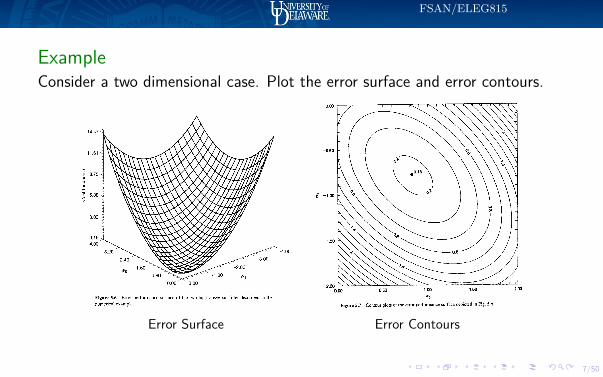
ExampleConsider a two dimensional case. Plot the error surface and error contours.
Error Surface Error Contours

8/50
FSAN/ELEG815
Aside (Matrix Differentiation, Real Case):Let w ∈R(d+1) and let f : R(d+1)→R. The derivative of f (called gradient off) with respect to w is:
∇w(f) = ∂f
∂w =
∇0(f)∇1(f)
...∇d(f)
=
∂f∂w0∂f∂w1...∂f∂wd
Thus,
∇k(f) = ∂f
∂wk, k = 0,1, · · · ,d
9/50
FSAN/ELEG815
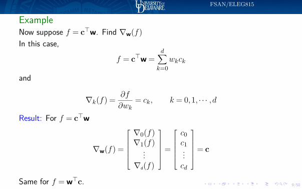
ExampleNow suppose f = c>w. Find ∇w(f)In this case,
f = c>w =d∑
k=0wkck
and
∇k(f) = ∂f
∂wk= ck, k = 0,1, · · · ,d
Result: For f = c>w
∇w(f) =
∇0(f)∇1(f)
...∇d(f)
=
c0c1...cd
= c
Same for f = w>c.

10/50
FSAN/ELEG815
ExampleLastly, suppose f = w>Qw. Where Q ∈ R(d+1)×(d+1) and w ∈ Rd+1. Find∇w(f)In this case, using the product rule:
∇wf = ∂w>(Qw)∂w + ∂(w>Q)w
∂w
= ∂w>u1∂w + ∂u>2 w
∂w
Using previous result, ∂c>w∂w = ∂w>c
∂w = c,
∇wf = u1 +u2,
= Qw+Q>w = (Q+Q>)w, if Q symmetric, Q> = Q= 2Qw
11/50
FSAN/ELEG815
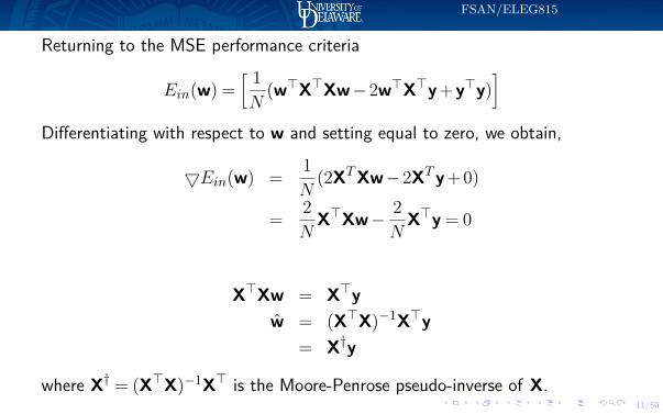
Returning to the MSE performance criteria
Ein(w) =[ 1N
(w>X>Xw−2w>X>y+y>y)]
Differentiating with respect to w and setting equal to zero, we obtain,
5Ein(w) = 1N
(2XTXw−2XTy+ 0)
= 2NX>Xw− 2
NX>y = 0
X>Xw = X>yw = (X>X)−1X>y
= X†y
where X† = (X>X)−1X> is the Moore-Penrose pseudo-inverse of X.

12/50
FSAN/ELEG815
Summarizing
1 x11 x12 · · · x1d... ... ... . . . ...1 xN1 xN2 · · · xNd
︸ ︷︷ ︸X: age, gender, anual salary...
·
w0w1...wd
︸ ︷︷ ︸
w: parameters
=
y1...yN
︸ ︷︷ ︸
y: credit line ($)
Linear system of equations:
X︸︷︷︸known
w︸︷︷︸solve
= y︸︷︷︸known
w = (X>X)−1X>y= X†y
where X† is the Moore-Penrose pseudo-inverse of X.
13/50
FSAN/ELEG815
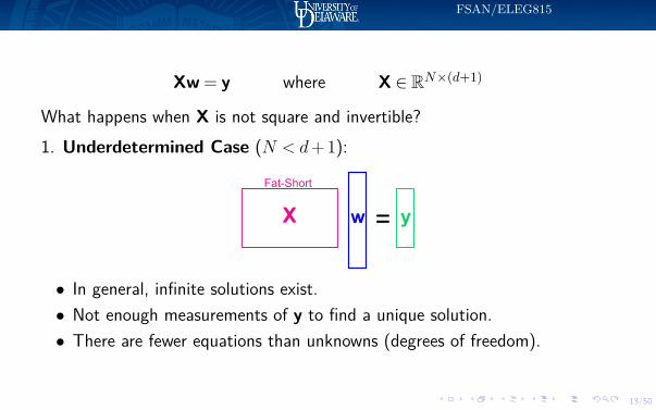
Xw = y where X ∈ RN×(d+1)
What happens when X is not square and invertible?1. Underdetermined Case (N < d+ 1):
X
Fat-Short
yw
• In general, infinite solutions exist.• Not enough measurements of y to find a unique solution.• There are fewer equations than unknowns (degrees of freedom).
14/50
FSAN/ELEG815
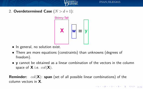
2. Overdetermined Case (N > d+ 1):
X
Skinny-Tall
w y
• In general, no solution exist.• There are more equations (constraints) than unknowns (degrees offreedom).• y cannot be obtained as a linear combination of the vectors in the columnspace of X i.e. col(X).
Reminder: col(X): span (set of all possible linear combinations) of thecolumn vectors in X.

15/50
FSAN/ELEG815
Moore-Penrose Pseudo-inverse with SVDSVD allows us to "invert" X. GivenX = UΣV> and the linear model:
Xw = yUΣV>w = y
Multiplying both sides by U>:
U>UΣV>w = U>y where U>U = IΣV>w = U>y
Multiplying both sides by Σ−1 :
Σ−1ΣV>w = Σ−1U>y where Σ−1Σ = IV>w = Σ−1U>y

16/50
FSAN/ELEG815
Solving with SVD
V>w = Σ−1U>y
Multiplying both sides by V:
VV>w = VΣ−1U>y where VV> = Iw = VΣ−1U>y
Then
w = VΣ−1U>yw = X†y
where X† = VΣ−1U is the Moore-Penrose pseudo-inverse of X.
17/50
FSAN/ELEG815
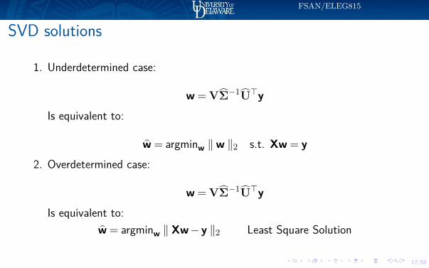
SVD solutions
1. Underdetermined case:
w = VΣ−1U>yIs equivalent to:
w = argminw ‖w ‖2 s.t. Xw = y2. Overdetermined case:
w = VΣ−1U>yIs equivalent to:
w = argminw ‖ Xw−y ‖2 Least Square Solution

18/50
FSAN/ELEG815
A real data set
16x16 pixels gray-scale images of digits from the US Postal Service Zip CodeDatabase. The goal is to recognize the digit in each image.
This is not a trivial task (even for a human). A typical human error Eout isabout 2.5% due to common confusions between 4,9 and 2,7.
Machine Learning tries to achieve or beat this error.
19/50
FSAN/ELEG815
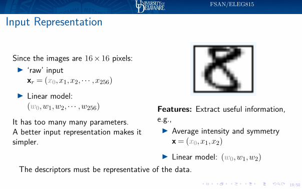
Input Representation
Since the images are 16×16 pixels:I ‘raw’ input
xr = (x0,x1,x2, · · · ,x256)
I Linear model:(w0,w1,w2, · · · ,w256)
It has too many many parameters.A better input representation makes itsimpler.
Features: Extract useful information,e.g.,I Average intensity and symmetry
x = (x0,x1,x2)
I Linear model: (w0,w1,w2)The descriptors must be representative of the data.
20/50
FSAN/ELEG815
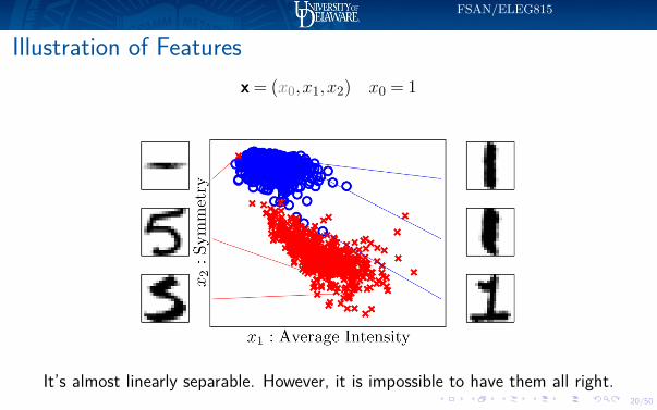
Illustration of Featuresx = (x0,x1,x2) x0 = 1
It’s almost linearly separable. However, it is impossible to have them all right.
21/50
FSAN/ELEG815
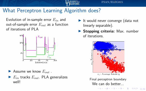
What Perceptron Learning Algorithm does?Evolution of in-sample error Ein andout-of-sample error Eout as a functionof iterations of PLA
I Assume we know Eout .I Ein tracks Eout. PLA generalizes
well!
I It would never converge (data notlinearly separable).
I Stopping criteria: Max. numberof iterations.
Final perceptron boundaryWe can do better...

22/50
FSAN/ELEG815
Classification boundary - PLA versus Poket
PLA Pocket
23/50
FSAN/ELEG815
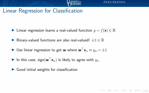
Linear Regression for Classification
I Linear regression learns a real-valued function y = f(x) ∈ R
I Binary-valued functions are also real-valued! ±1 ∈ R
I Use linear regression to get w where w>xn ≈ yn =±1
I In this case, sign(w>xn) is likely to agree with yn
I Good initial weights for classification

24/50
FSAN/ELEG815

25/50
FSAN/ELEG815
Example: Boston Housing Market• Predict y: Median value of home in thousands.• y = w>x• x: 13 attributes correlated with house price.

26/50
FSAN/ELEG815
Boston Housing Dataset (1970)

27/50
FSAN/ELEG815
ExampleColumns like CRIM, ZN, RM, B seems to have outliers. Let’s see the outlierspercentage in every column:

28/50
FSAN/ELEG815
Example:Predicted house value (y) and the true house value (y):
0 100 200 300 400 500-10
0
10
20
30
40
50
Med
iam
hom
e va
lue
($1k
)
0 100 200 300 400 500-10
0
10
20
30
40
50
Med
iam
hom
e va
lue
($1k
)Unsorted data Sorted Data

29/50
FSAN/ELEG815
Example
CRIM ZN
INDUS
CHASNOX
RMAGE
DISRAD
TAX
PTRATIO B
LSTAT
MEDV
Attribute
-2.5
-2
-1.5
-1
-0.5
0
0.5
1
Sig
nific
ance

30/50
FSAN/ELEG815
Definition (Steepest Descent (SD))Steepest descent, also known as gradient descent is an iterative technique forfinding the local minimum of a function.Given an arbitrary starting point, the current location (value) is moved insteps proportional to the negatives of the gradient at the current point.I SD is an old, deterministic method, that is the basis for stochastic
gradient based methodsI SD is a feedback approach to finding local minimum of an error surfaceI The error surface must be known a prioriI In the MSE case, SD converges converges to the optimal solution without
inverting a matrix

31/50
FSAN/ELEG815
ExampleConsider a well structured cost function with a single minimum. Theoptimization proceeds as follows:
Contour plot showing that evolution of the optimization

32/50
FSAN/ELEG815
To derive the approach, consider:
Ein = 1N||Xw−y||22
= 1N
(y>y−y>Xw−w>X>y+w>X>Xw)
= σ2y−p>w−w>p+w>Rw
whereσ2y = 1
N y>y variance estimate of desired signal
p = 1NX>y – cross-correlation estimate between x and y
R = 1NX>X – correlation matrix estimate of x

33/50
FSAN/ELEG815
When w is set to the (optimal) Least Squares solution w0:
w = w0 = R−1p
andEin = Einmin = σ2
y−pHw0
I Use the method of steepest descent to iteratively find w0.I The optimal result is achieved since the cost function is a second order
polynomial with a single unique minimum

34/50
FSAN/ELEG815
ExampleThe MSE is a bowl–shaped surface, which is a function of the 2-D spaceweight vector w(n)
Surface PlotContour Plot
Imagine dropping a marble at any point on the bowl-shaped surface.The ball will reach the minimum point by going through the path of steepestdescent.
35/50
FSAN/ELEG815
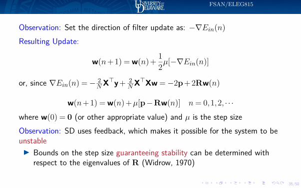
Observation: Set the direction of filter update as: −∇Ein(n)Resulting Update:
w(n+ 1) = w(n) + 12µ[−∇Ein(n)]
or, since ∇Ein(n) =− 2NX>y+ 2
NX>Xw =−2p+ 2Rw(n)
w(n+ 1) = w(n) +µ[p−Rw(n)] n= 0,1,2, · · ·where w(0) = 0 (or other appropriate value) and µ is the step sizeObservation: SD uses feedback, which makes it possible for the system to beunstableI Bounds on the step size guaranteeing stability can be determined with
respect to the eigenvalues of R (Widrow, 1970)
36/50
FSAN/ELEG815
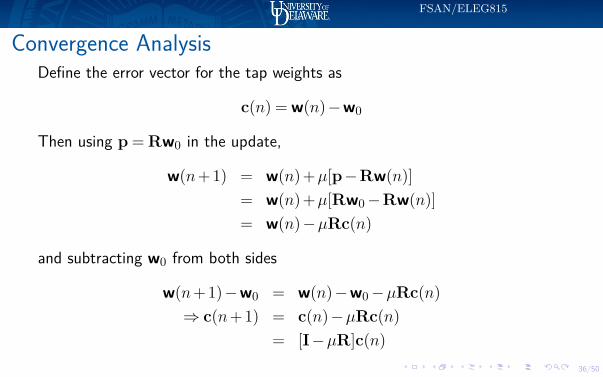
Convergence AnalysisDefine the error vector for the tap weights as
c(n) = w(n)−w0
Then using p = Rw0 in the update,
w(n+ 1) = w(n) +µ[p−Rw(n)]= w(n) +µ[Rw0−Rw(n)]= w(n)−µRc(n)
and subtracting w0 from both sides
w(n+ 1)−w0 = w(n)−w0−µRc(n)⇒ c(n+ 1) = c(n)−µRc(n)
= [I−µR]c(n)

37/50
FSAN/ELEG815
Using the Unitary Similarity Transform
R = QΩΩΩQH
we have
c(n+ 1) = [I−µR]c(n)= [I−µQΩΩΩQH ]c(n)
⇒QHc(n+ 1) = [QH −µQHQΩΩΩQH ]c(n)= [I−µΩΩΩ]QHc(n) (∗)
Define the transformed coefficients as
v(n) = QHc(n)= QH(w(n)−w0)
Then (∗) becomesv(n+ 1) = [I−µΩΩΩ]v(n)

38/50
FSAN/ELEG815
Consider the initial condition of v(n)
v(0) = QH(w(0)−w0)= −QHw0 [if w(0) = 0]
Consider the kth term (mode) in
v(n+ 1) = [I−µΩΩΩ]v(n)
I Note [I−µΩΩΩ] is diagonalI Thus all modes are independently updatedI The update for the kth term can be written as
vk(n+ 1) = (1−µλk)vk(n) k = 1,2, · · · ,M
or using recursionvk(n) = (1−µλk)nvk(0)

39/50
FSAN/ELEG815
Observation: Conversion to the optimal solution requires
limn→∞w(n) = w0
⇒ limn→∞c(n) = lim
n→∞w(n)−w0 = 0
⇒ limn→∞v(n) = lim
n→∞QHc(n) = 0⇒ lim
n→∞vk(n) = 0 k = 1,2, · · · ,M (∗)
Result: According to the recursion
vk(n) = (1−µλk)nvk(0)
the limit in (∗) holds if and only if
|1−µλk|< 1 for all k
Thus since the eigenvalues are nonnegative, 0< µλmax < 2, or
0< µ <2
λmax

40/50
FSAN/ELEG815
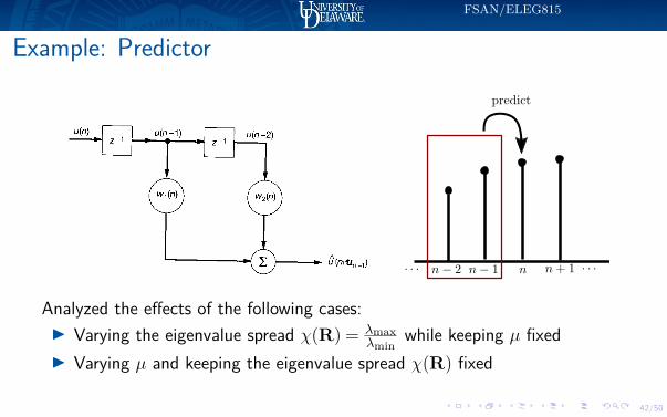
Example: Predictor
Consider a two–tap predictor for real–valued input

41/50
FSAN/ELEG815
Example: PredictorUse x(n−1) =
[x(n−1)x(n−2)
]to predict x(n) such that
y(n) = x(n) = x(n−1)>[w1(n)w2(n)
]= x(n−1)>w(n)
Xw = yx(2) x(1)x(3) x(2)... ...
x(n−1) x(n−2)
︸ ︷︷ ︸
X∈RN×2
[w1w2
]=
x(3)x(4)...
x(n)
︸ ︷︷ ︸
y∈RN
R = 1NX
TX p = 1NX
Ty
42/50
FSAN/ELEG815
Example: Predictor
Analyzed the effects of the following cases:I Varying the eigenvalue spread χ(R) = λmax
λminwhile keeping µ fixed
I Varying µ and keeping the eigenvalue spread χ(R) fixed
43/50
FSAN/ELEG815
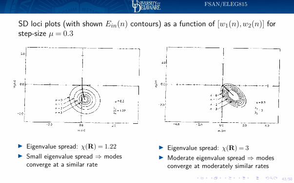
SD loci plots (with shown Ein(n) contours) as a function of [w1(n),w2(n)] forstep-size µ= 0.3
I Eigenvalue spread: χ(R) = 1.22I Small eigenvalue spread ⇒ modes
converge at a similar rate
I Eigenvalue spread: χ(R) = 3I Moderate eigenvalue spread ⇒ modes
converge at moderately similar rates

44/50
FSAN/ELEG815
SD loci plots (with shown Ein(n) contours) as a function of [w1(n),w2(n)] forstep-size µ= 0.3
I Eigenvalue spread: χ(R) = 10I Large eigenvalue spread ⇒ modes
converge at different rates
I Eigenvalue spread: χ(R) = 100I Very large eigenvalue spread ⇒ modes
converge at very different ratesI Principle direction convergence is fastest
45/50
FSAN/ELEG815
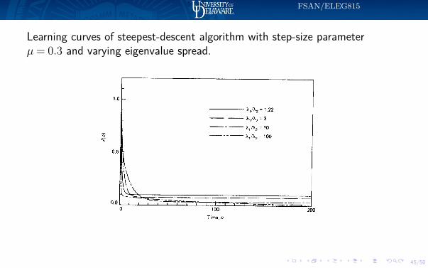
Learning curves of steepest-descent algorithm with step-size parameterµ= 0.3 and varying eigenvalue spread.

46/50
FSAN/ELEG815
SD loci plots (with shown Ein(n) contours) as a function of [w1(n),w2(n)]with χ(R) = 10 and varying step–sizes
I Step–sizes: µ= 0.3I This is over–damped ⇒ slow
convergence
I Step–sizes: µ= 1I This is under–damped ⇒ fast (erratic)
convergence

47/50
FSAN/ELEG815
Stochastic Gradient Descent (SGD)Instead of considering the full batch, for each iteration, pick one training datapoint (Xn,yn) at random and apply GD update to e(h(xn,yn))The weight update of SGD is:
w(t+ 1) = w(t)−η∇en(w(t))
For e(h(xn,yn)) = (w>xn−yn)2 i.e. for the mean squared error:
∇en(w) = 2xn(w>xn−yn) w>xn = x>nw= 2xn(x>nw−yn)= 2(xnx>nw−xnyn)= 2(Rw− p)
where R = xnx>n is the instantaneous estimate of R and p = xnyn is theinstantaneous estimate of p.
48/50
FSAN/ELEG815
Stochastic Gradient Descent (SGD)
Since n is picked at random, the expected weight change is:
En [−∇e(h(xn,yn))] = 1N
N∑n=1−∇e(h(xn,yn))
= −∇Ein
Same as the batch gradient descent.
Result: On ‘average’ the minimization proceeds in the right direction(remember LMS).

49/50
FSAN/ELEG815
Stochastic Gradient Descent (SGD)Instead of considering the full batch, for each iteration, pick one training datapoint (xn,yn) at random and apply GD update to e(h(xn,yn))The weight update of SGD is:
w(t+ 1) = w(t)−η∇en(w(t))
Since n is picked at random, the expected weight change is:
En [−∇e(h(xn,yn))] = 1N
N∑n=1−∇e(h(xn,yn))
= −∇Ein
Same as the batch gradient descent.
Result: On ‘average’ the minimization proceeds in the right direction.

50/50
FSAN/ELEG815
Benefits of SGD1. Cheaper computation (by
a factor of N compare toGD)
2. Randomization3. Simple
Rule of thumb:Start with:
η = 0.1 works!
Randomization helps to avoid local minima and flatregions.
SGD is successful in practice!