Embed Size (px)
Citation preview
From the Inside Out – Applicationof the Mass Balance Model for PM
Exposure Assessment in ResidentialSettings Under the Influencesof Indoor and Outdoor Factors
The Harvard community has made thisarticle openly available. Please share howthis access benefits you. Your story matters
Citation Lee, Wan-Chen. 2015. From the Inside Out – Application of the MassBalance Model for PM Exposure Assessment in Residential SettingsUnder the Influences of Indoor and Outdoor Factors. Doctoraldissertation, Harvard T.H. Chan School of Public Health.
Citable link http://nrs.harvard.edu/urn-3:HUL.InstRepos:23205179
Terms of Use This article was downloaded from Harvard University’s DASHrepository, and is made available under the terms and conditionsapplicable to Other Posted Material, as set forth at http://nrs.harvard.edu/urn-3:HUL.InstRepos:dash.current.terms-of-use#LAA
FROM THE INSIDE OUT – APPLICATION OF THE MASS BALANCE MODEL FOR
PM EXPOSURE ASSESSMENT IN RESIDENTIAL SETTINGS UNDER THE
INFLUENCES OF
INDOOR AND OUTDOOR FACTORS
WAN-CHEN LEE
A Dissertation Submitted to the Faculty of
The Harvard T.H. Chan School of Public Health
in Partial Fulfillment of the Requirements
for the Degree of Doctor of Science
in the Department of Environmental Health
Harvard University
Boston, Massachusetts
November, 2015
ii
Dissertation Advisor: Dr. Petros Koutrakis Wan-Chen Lee
From the Inside Out – Application of the Mass Balance Model for PM Exposure
Assessment in Residential Settings under the Influences of Indoor and Outdoor Factors
Abstract
The application of the widely used mass balance model in determining portable air purifier
(PAP) effectiveness in particulate matter (PM) removal was not validated in occupied residential
settings. The corresponding size-resolved information and measurements for the model
parameters and PAP effectiveness were also limited to better characterize human exposure to
indoor PM. Additionally, effects of ambient factors, such as meteorology, and their long-term
impacts on occupant indoor exposure to outdoor PM was unclear.
We achieved well-mixed environment and steady state of PM concentrations that met the
mass balance model assumptions. Size-resolved particle deposition rate was determined using
non-linear mixed effects model, whereas linear mixed effects model was used to estimate the
slope between the measured and modeled effectiveness for validation purpose.
To evaluate the impact of ambient factors on PM exposure, we assembled data from two
cohorts in the greater Boston area, assessing the monthly and long-term effect of temperature and
other meteorology on Sr. Long-term meteorology was projected using 15 weather models for the
past and future 20 years to estimate Sr for the corresponding periods with mixed effects models.
Both particle deposition rate and portable air purifier effectiveness were highly particle size-
dependent. Filtration was found to be the dominant removal mechanism for submicrometer
particles, whereas deposition could play a more important role in ultrafine particle removal.
iii
There was reasonable agreement between measured and modeled effectiveness with size-
resolved slopes ranging from 1.11±0.06 to 1.25±0.07 (mean±SE), except for particles <35 nm.
Sr was found to be a robust measure of indoor exposure to outdoor PM, and temperature was
its significant predictor. Seasonal effect of temperature was much more dominant when
compared to long-term effect on Sr, which differed in the whole population and the
subpopulation of naturally ventilated homes. However, long-term temperature effect was small,
with maximum of <10% for summer Sr compared to the past.
Findings from the studies improved characterization of indoor PM exposure. The study
design and methods can be used in the future to better understand exposure scenarios and their
correlation to health effects in other homes or populations.

iv
TABLE OF CONTENTS
LIST OF FIGURES ............................................................................................................ vi
LIST OF TABLES .............................................................................................................. ix
ACKNOWLEDGEMENTS ............................................................................................... x
INTRODUCTION ............................................................................................................... 1
Bibliography ..................................................................................... 10
CHAPTER 1 Size-Resolved Deposition Rates for Ultrafine and Submicrometer
Particles in a Residential Housing Unit ........................................ 16
Environmental Science & Technology. 2014, 48 (17), 10282–10290
Abstract ............................................................................................. 17
Introduction ....................................................................................... 18
Materials and methods ...................................................................... 20
Results ............................................................................................... 27
Discussion ......................................................................................... 32
Bibliography ..................................................................................... 42
Supporting information (SI) .............................................................. 46
CHAPTER 2 Validation and Application of the Mass Balance Model to Determine
the Effectiveness of Portable Air Purifiers in Removing Ultrafine and
Submicrometer Particles in an Apartment ................................... 55
Environmental Science & Technology. (Published online, July 24th, 2015)
Abstract ............................................................................................. 56
Introduction ....................................................................................... 57
Materials and methods ...................................................................... 58
v
Results ............................................................................................... 66
Discussion ......................................................................................... 73
Bibliography ..................................................................................... 78
Supporting information (SI) .............................................................. 83
CHAPTER 3 Effects of Monthly and Long-term Temperature Change on Indoor
Exposure to Outdoor PM2.5 in the Greater Boston Area ............ 102
(Working paper)
Abstract ............................................................................................. 103
Introduction ....................................................................................... 104
Materials and Methods ...................................................................... 106
Results ............................................................................................... 113
Discussion ......................................................................................... 126
Bibliography ..................................................................................... 132
CONCLUSIONS ............................................................................................................ 138
vi
LIST OF FIGURES
Figure 0.1 A schematic illustrating the scope of the overall dissertation.
Figure 0.2 A schematic illustrating the connections between Chapter 1, 2, and 3 based on the mass balance model application.
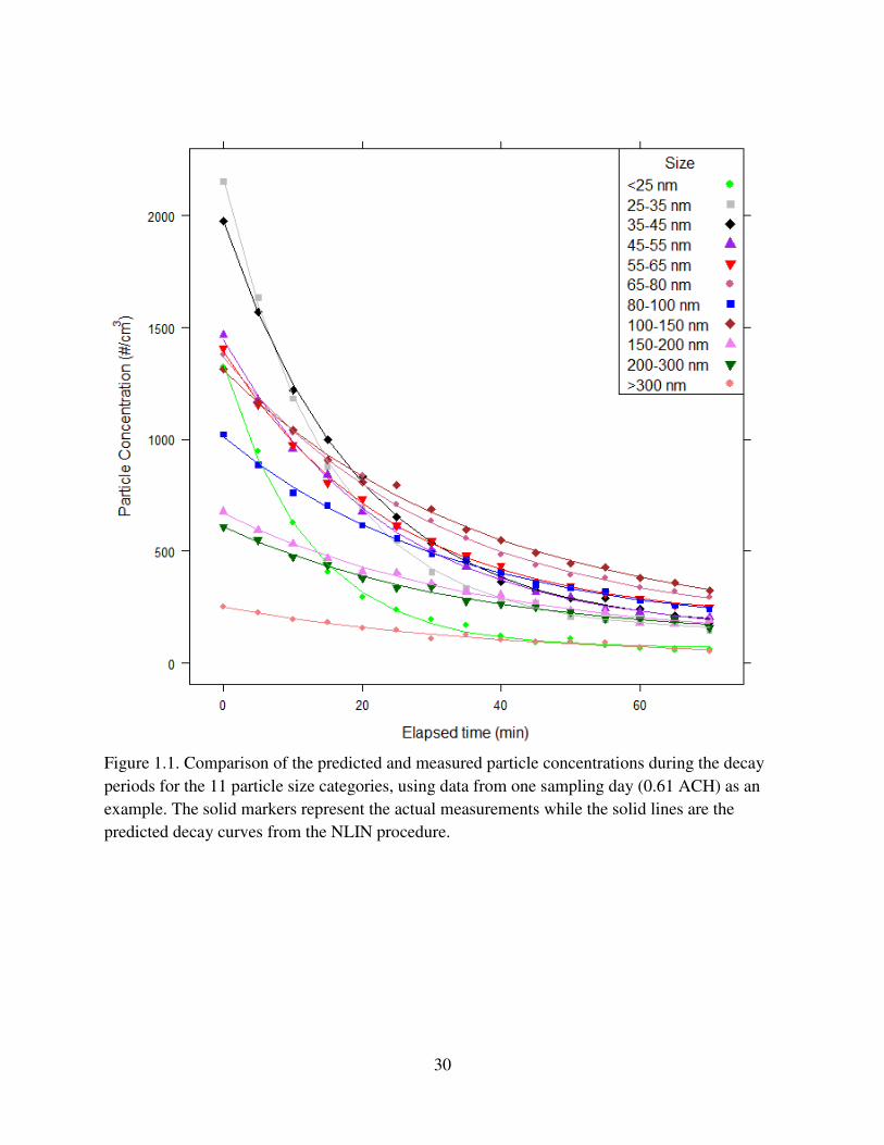
Figure 1.1 Comparison of the predicted and measured particle concentrations during the decay periods for the 11 particle size categories, using data from one sampling day (0.61 ACH) as an example. The solid markers represent the actual measurements while the solid lines are the predicted decay curves from the NLIN procedure.
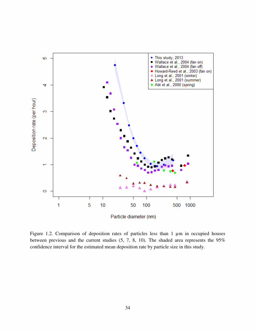
Figure 1.2 Comparison of deposition rates of particles less than 1 µm in occupied houses between previous and the current studies. The shaded area represents the 95% confidence interval for the estimated mean deposition rate by particle size in this study.
Figure 2.1 Layout of the devices and instruments in the apartment.
Figure 2.2 Average size-resolved filtration efficiencies of the 2 PAPs under 3 flow settings.
Figure 2.3 An example of the continuous measurements and device operation profiles over one sampling day at g=0.91 h-1 for the total particle concentration (系岫建岻), the total particle generation rate (荊継痛墜痛銚鎮), the total flow rate of the 2 PAPs (芸捗), and the 鯨繋滞 concentration.
Figure 2.4 Size-resolved particle removal rates: filtration by PAPs, deposition, and air exchange. 系畦迎迎沈 (h-1) is the size-resolved clean air replacement rate, equal to 系畦経迎沈【撃. 系畦迎迎な, 系畦迎迎に and 系畦迎迎ぬ corresponded to the flow rates of 195, 387, and 540 m3/h, respectively. The air exchange rates were the average values under three target air exchange rates: ACH1, ACH2, and ACH3 are the target air exchange rate of 0.60, 0.90, and 1.20 h-1, respectively. k1, k2 and k3 are the average particle deposition rates at ACH1, ACH2, and ACH3, respectively.
Figure 2.5 Measured size-resolved effectiveness for the three PAP flow rates (芸捗= 195, 387, and 540 m3/h) under three target air exchange rates (A=0.60, 0.90 and1.20 h-1).
Figure 2.6 The slopes and their 95% confidence intervals by particle size obtained from the mixed effects model. The shaded area represents ±10% of the ideal coefficient of 1 (0.90-1.10).
Figure 2.7 Relationship between effectiveness and CARR.
Figure 3.1 Boxplots for Sr measurements by month for (a) the whole population with mixed AC usage, and (b) the subpopulation of naturally ventilated homes (AC=0). The
vii
solid points represent the Sr observations; whereas the filled diamonds in red represent the monthly mean of Sr.
Figure 3.2 Sr measurement for (a) the subpopulation of naturally ventilated homes (AC=0),
and (b) homes that used AC during the sampling period (AC=1). Measurements
from the two cohorts are marked in different colors.
Figure 3.3 Comparisons between projected monthly mean temperature, RH, wind speed and precipitation from CMIP5 models and NARR database for the period of 1981-2000.
Figure 3.4 Mean temperature by month for the past and the future based on paired years
(N=1 to 20). The solid and dashed lines are projections for the future and the past,
respectively. The light-colored lines represent projections from the CMIP5
models, whereas the dark-colored lines describe the multi-model means across the
CMIP5 models.
Figure 3.5 Mean estimated Sr by month for the past and the future based on paired years
(N=1 to 20) for the whole population with mixed AC usage (AC=mixed). The
solid and dashed lines are projections for the future and the past, respectively. The
light-colored lines represent projections from the CMIP5 models, whereas the
dark-colored lines describe the multi-model means across the CMIP5 models.
Figure 3.6 Mean estimated Sr by month for the past and the future based on paired years (N=1 to 20) for the subpopulation of naturally ventilated homes (AC=0). The solid and dashed lines are projections for the future and the past, respectively. The light-colored lines represent projections from the CMIP5 models, whereas the dark-colored lines describe the multi-model means across the CMIP5 models.
Figure 3.7 Projected monthly mean temperature for the past (1981-2000) and the future (2046-2065) by 15 CMIP5 models (dashed lines). The solid line is the overall monthly mean across the CMIP5 models.
Figure 3.8 Predicted monthly mean Sr for the past and the future by the two populations. The
solid lines were the overall monthly mean across the CMIP5 models while the
dashed lines were 罰 1 SD from the overall mean. AC=0 represented the
subpopulation of naturally ventilated homes and AC=mixed was referred to the
whole population.
Figure 3.9 Difference in predicted monthly mean Sr between the two populations for the past
and the future. The solid lines are the overall monthly mean difference across the
CMIP5 models while the dashed lines are 罰 1 SD from the overall mean. AC=0
viii
represents the subpopulation of naturally ventilated homes and AC=mixed is
referred to the whole population.
Figure 3.10 Monthly mean differences in estimates between the future and the past for (a) temperature, and (b) Sr. The solid lines are the overall monthly mean difference across the CMIP5 models while the dashed lines are 罰 1 SD from the overall mean. AC=0 represents the subpopulation of naturally ventilated homes and AC=mixed is referred to the whole population.
ix
LIST OF TABLES
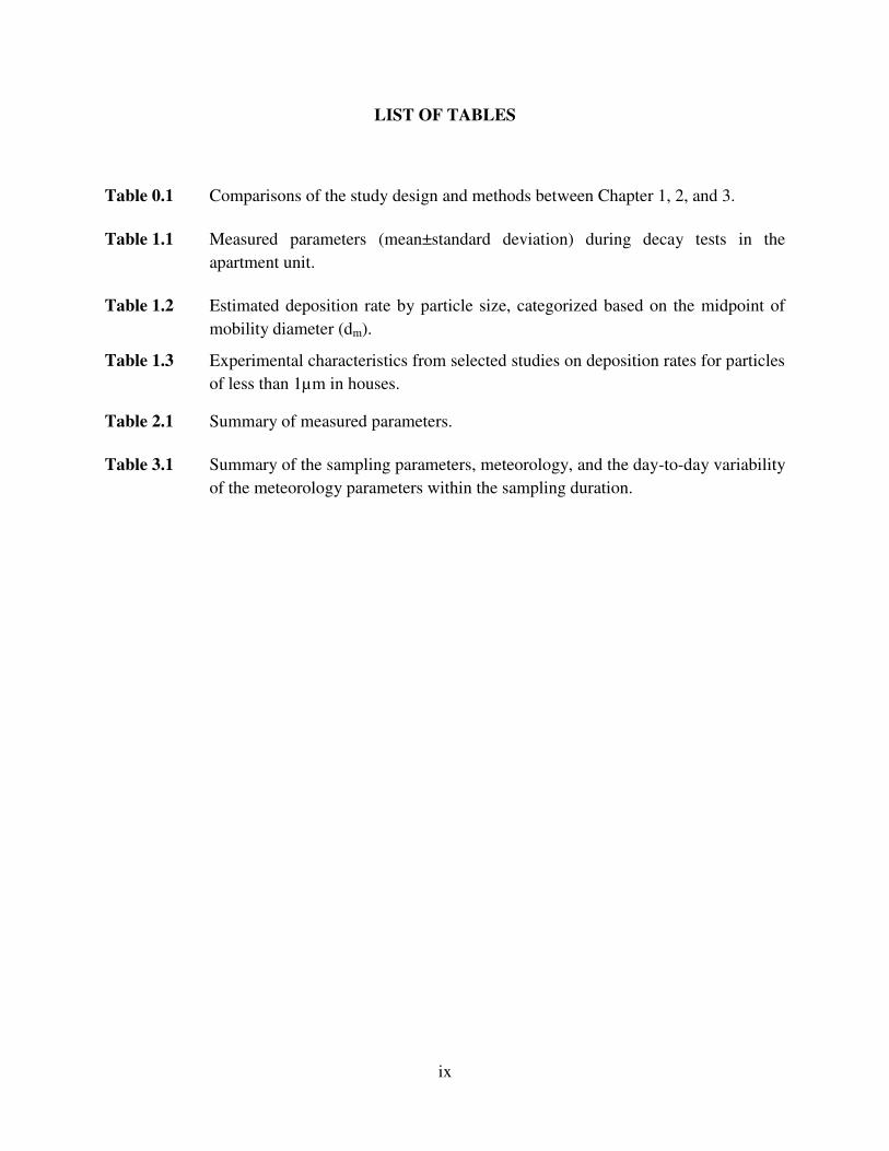
Table 0.1 Comparisons of the study design and methods between Chapter 1, 2, and 3.
Table 1.1 Measured parameters (mean±standard deviation) during decay tests in the
apartment unit.
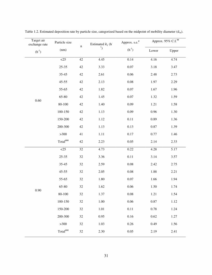
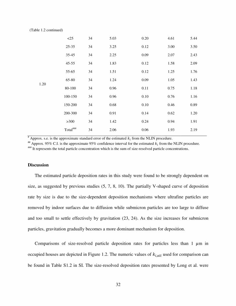
Table 1.2 Estimated deposition rate by particle size, categorized based on the midpoint of
mobility diameter (dm).
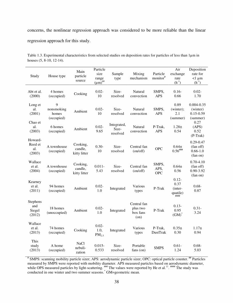
Table 1.3 Experimental characteristics from selected studies on deposition rates for particles
of less than 1µm in houses.
Table 2.1 Summary of measured parameters.
Table 3.1 Summary of the sampling parameters, meteorology, and the day-to-day variability
of the meteorology parameters within the sampling duration.

x
ACKNOWLEDGEMENTS
First of all, I would like to thank my advisor Dr. Petros Koutrakis for his patience and for
granting me the freedom to pursue research ideas and explore different approaches. Through his
guidance I have learned and equipped myself with skills and strength to mature as an
independent researcher.
I would also like to express my deepest gratitude to my research committee members, Dr.
Stephen Rudnick and Dr. Paul Catalano, who have provided invaluable insights and knowledge
in steering me towards the right direction for my study, and from whom I have gained friendship
and tremendous support.
My extended appreciation goes to the Taiwan Ministry of Education for the financial support
in the first three years of my doctoral program, and Coway Ltd. for the partial sponsorship of the
air purifier study in this dissertation. I am also thankful to Dr. Loretta Mickley and her team for
the effective collaboration in the climate change study.
Furthermore, I would like to acknowledge Mike Wolfson, Joy Lawrence, and Steve Ferguson
for their technical support in research design and methods, which helped establish a solid
foundation for successfully carrying out the field work. Mike has been a great mentor, and it was
such a pleasure and rewarding experience to work with him.
Last but not least, I’m profoundly indebted to my family and friends for their generous and
firm support through this journey, especially my parents and grandparents who have been so
strong and selfless for their sacrifices to help me reach this milestone.
Wan-Chen Lee
Boston, Massachusetts

1
INTRODUCTION
2
Epidemiological studies have shown significance of ambient particulate matter (PM)
exposure on health, most notably cardiovascular illness and mortality (1-3). Ambient PM can
penetrate indoor environment where people spend the majority of their time (4). Consequently,
indoor exposure to outdoor PM has been one of the central fields where researchers invest
themselves to unravel the relationship between the exposure and its resulting health risks from
the complex interactions of indoor, outdoor and human factor contributions.
Indoor PM concentration is a result of a dynamic process, featuring competing factors of
particle source emission (input) and removal (output) via various pathways, which can be
categorized into PM properties-related mechanisms, building characteristics, and occupant
behavior (5). One pollutant property-driven removal mechanism is size-dependent particle
deposition onto indoor surfaces. Both large and small particles have higher rates because larger
particles can settle by gravitation, whereas diffusion is the dominant mechanism for small
particles, such as ultrafine particles (6). Particles that have sizes between the two, mostly
submicrometer particles, tend to stay airborne because they are too large to diffuse and too small
to settle by gravitation. The size-resolved deposition rate can also be affected by air mixing and
the indoor surface area, with generally positive relationships (7, 8). Given proper experimental
design and instruments, particle deposition rates can be measured readily on site.
Similarly, penetration coefficient for outdoor PM entering indoors through building cracks is
also size-dependent (9, 10). During infiltration process, small particles are removed by diffusion,
whereas larger particles are removed both by gravitational settling and inertial impaction at the
crack entry (11). Penetration coefficient is affected by the geometry and roughness of cracks
(10). However, when penetration occurs through an open window, the coefficient is close to
unity.
3
Air through building cracks and windows, together with mechanical ventilation by fans, are
major mechanisms for building ventilation. Air exchange rate is used as measure to quantify
ventilation when there is exchange of air between indoors and outdoors. Its effect is
bidirectional, and thus it is commonly used to adjust the indoor PM concentrations. For example,
occupants close windows to minimize air exchange and the penetration of ambient particle in
high outdoor pollution episodes (e.g., forest fire) (12, 13). Contrarily, windows are open to vent
pollutants from significant indoor sources such as smoking or cooking (14). For naturally
ventilated buildings, wind speed, and indoor-outdoor temperature difference are also factors
influencing ACH, in addition to the cracks and window opening (15-17). On the other hand, AC
usage has been reported to decrease ACH through closed windows and removal by deposition
and/or additional filters inside the AC system (15, 18, 19).
Various indoor sources have been characterized for their contributions to indoor PM
concentrations, particle composition and size distribution. Emission from these sources is often
intermittent/episodic, highly variable, and tightly related to occupant activities, such as cooking,
cleaning (e.g., vacuuming), smoking, and incense burning (20-22). When present, indoor sources
tend to result in PM concentrations much higher than that from outdoors, partially due to intense
source strength and small air dilution volume of indoor space (20, 23).
In view of the omnipresent indoor particle exposure from various sources with relatively
modest natural removal mechanisms, some intervention strategies aim to more effectively reduce
overall indoor PM concentration, regardless of the sources. Houses built more recently are often
equipped with the central air system, inside which some houses install filters for particle
removal. For naturally ventilated homes, portable air purifiers can be useful (13, 24, 25). The
purifiers are designed with different flow rates and various technologies, such as filtration,
4
electrostatic precipitation, and ion generation (26, 27). Studies have shown that those equipped
with high efficiency particulate air (HEPA) filter and electrostatic precipitators are the most
effective, depending on the particle size (27-29). However, electrostatic precipitators were found
to generate ozone which is a harmful pollutant (26).
Given diverse residential indoor environment and varying occupant activity pattern, a
systematic and comprehensive understanding of the aforementioned mechanisms not only help
separate the contribution of indoor and outdoor sources, but also assist in epidemiological studies
to link PM exposure and interventions to observed health outcomes or benefits on the population
level. The mass balance equation is one such means to describe the relationship between indoor
PM concentration and the source contribution. The resulting mass balance model (MBM), often
referred as the box model, has been a common approach for determining the indoor factors that
influence indoor PM, and sometimes the PM concentration itself in homes (16, 20, 30-32). These
factors include the ones previously discussed.
Indoor-outdoor PM ratio (I/O) derived from the mass balance equation in the absence of
indoor sources is often used as an index to quantitatively characterize particle infiltration and is
used to correlate personal exposure to outdoor PM concentrations (33). It is often referred to as
the infiltration factor. In epidemiological studies where indoor PM measurements of individual
homes are often unavailable, infiltration factor can be used to estimate the indoor PM
concentration of outdoor fraction given the ambient PM concentration from the central site.
Building tightness is one important factor for infiltration factor variability. With regard to
ambient factors, mainly meteorology, studies have shown that ambient temperature is associated
with occupant window opening behavior, which in turn could affect the air exchange rate and
increase particle infiltration (34, 35).
5
Substantial amount of research have been conducted to better understand the roles of indoor
factors and mechanisms as they contribute to indoor PM concentration through interactive,
competing or enhancive effects under the broad, yet complex framework of MBM application.
Gaps remain, however, not preventing from the development of knowledge, but to attenuate
generalizability or confidence in results interpretation due to uncertainties in findings or scarce
information in newly explored study areas. For example, the application of MBM in estimating
either the indoor PM or the other model parameters was not validated experimentally in
residential settings. Violation of mass balance assumptions in the homes could potentially lead to
biased predictions of PM related parameters. Additionally, size-resolved information is limited
for both model validation and the determined parameters such as deposition rate. While intensive
efforts have been placed in understanding how factors and mechanisms indoors influence human
exposure to PM in residences, ambient factors such as meteorology were less studied. Although
the change in specific meteorological parameters due to climate change was found to influence
ambient PM2.5 concentrations (36), there was very little information in the association between
meteorology and PM penetration to indoor environment.
Answers to these pending questions would strengthen the mass balance application in indoor
PM exposure assessment and improve the understanding of size-resolved behavior for those
particles. The main motivation of this dissertation is, therefore, to fill these existing gaps with
specific aspects on the protective removal mechanisms for indoor PM, and how the ambient
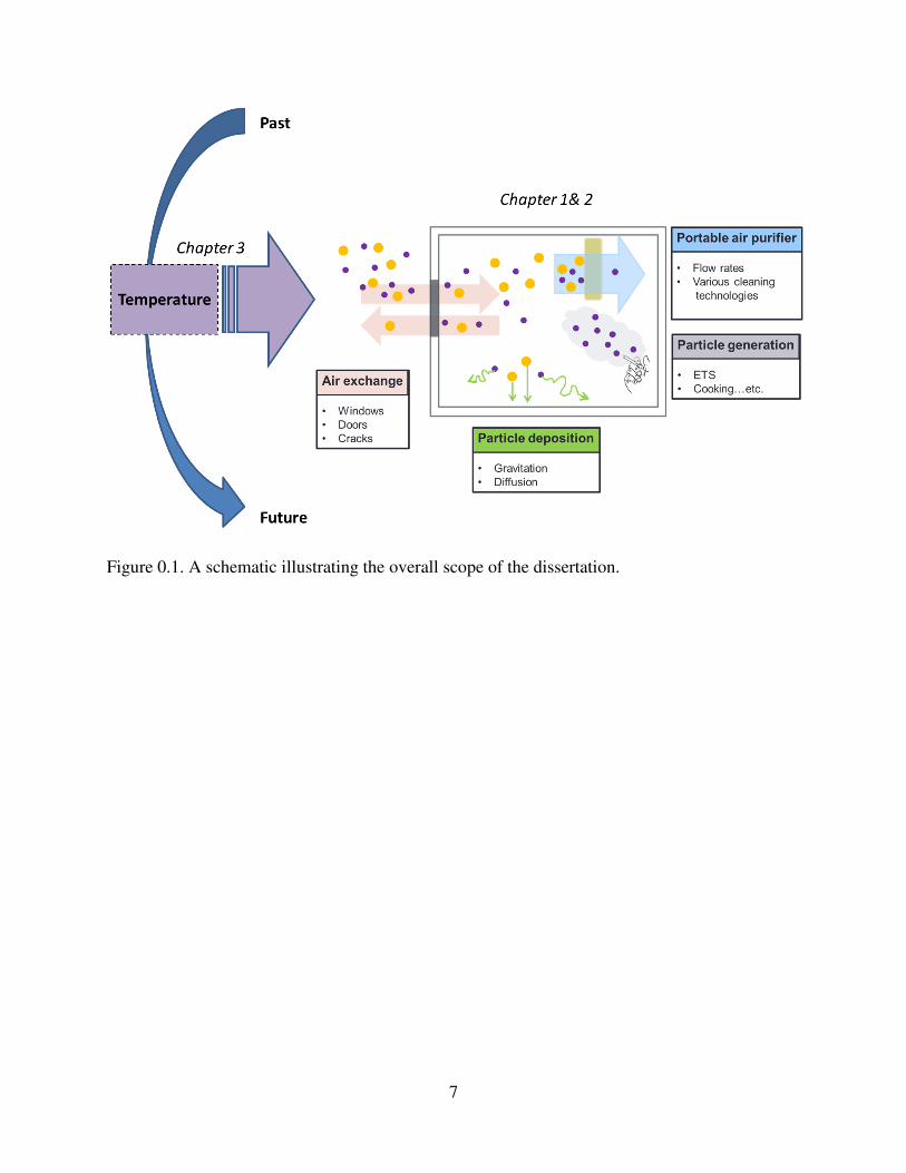
meteorology comes into play. Figure 0.1 and Figure 0.2 are provided to illustrate the overall
scope of this dissertation and the connections between the chapters.
Chapter 1 and 2 are embedded in the same controlled study which was conducted in an
apartment. Chapter 1 adopted a modified experimental approach, in conjunction with a MBM, to
6
determine the size-resolved deposition rates and assess the effect of air exchange rate under
enhanced mixing conditions. Chapter 2 aimed to validate the MBM through the assessment of
the size-resolved effectiveness of PAP(s) equipped with HEPA filters in removing ultrafine
particles (UFPs) (<0.1たm) and submicrometer particles (0.10−0.53 たm). Validation was done by
comparing experimentally determined size-resolved PAP effectiveness using directly measured
particle concentrations with and without the operation of PAPs, to the modeled effectiveness
using individually measured model input parameters during the same test periods.
In Chapter 3, the research focus was extended to factors outside the mass balance box (e.g.,
homes) to explore the impact of outdoor temperature and other meteorology on particle
infiltration factor on a monthly and long-term climate change basis, using archived samples from
two observational studies featuring 340 homes in the greater Boston area. Indoor-outdoor sulfur
ratio was used as a surrogate of infiltration factor for PM2.5 to associate with the main effect of
temperature with exposure models (mixed effects models). Weekly indoor-outdoor sulfur ratio
for the future and past 20 years were estimated using projected meteorology from 15 weather
forecast models, and were summarized into monthly averages. The predicted sulfur ratio were
also examined and compared across two population scenarios to reflect the influence of AC
usage: the whole population with mixed AC usage, and the subpopulation of naturally ventilated
homes.
Although studies in the three chapters all revolve around the mass balance equation, there are
some distinct differences in the study design, experimental development and statistical methods.
Table 0.1 shows a list of major comparisons.
7
Figure 0.1. A schematic illustrating the overall scope of the dissertation.
8
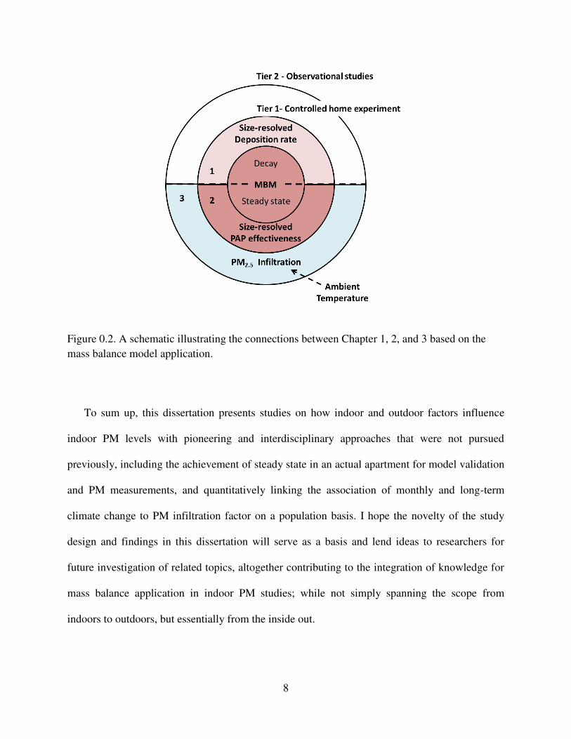
Figure 0.2. A schematic illustrating the connections between Chapter 1, 2, and 3 based on the
mass balance model application.
To sum up, this dissertation presents studies on how indoor and outdoor factors influence
indoor PM levels with pioneering and interdisciplinary approaches that were not pursued
previously, including the achievement of steady state in an actual apartment for model validation
and PM measurements, and quantitatively linking the association of monthly and long-term
climate change to PM infiltration factor on a population basis. I hope the novelty of the study
design and findings in this dissertation will serve as a basis and lend ideas to researchers for
future investigation of related topics, altogether contributing to the integration of knowledge for
mass balance application in indoor PM studies; while not simply spanning the scope from
indoors to outdoors, but essentially from the inside out.
9
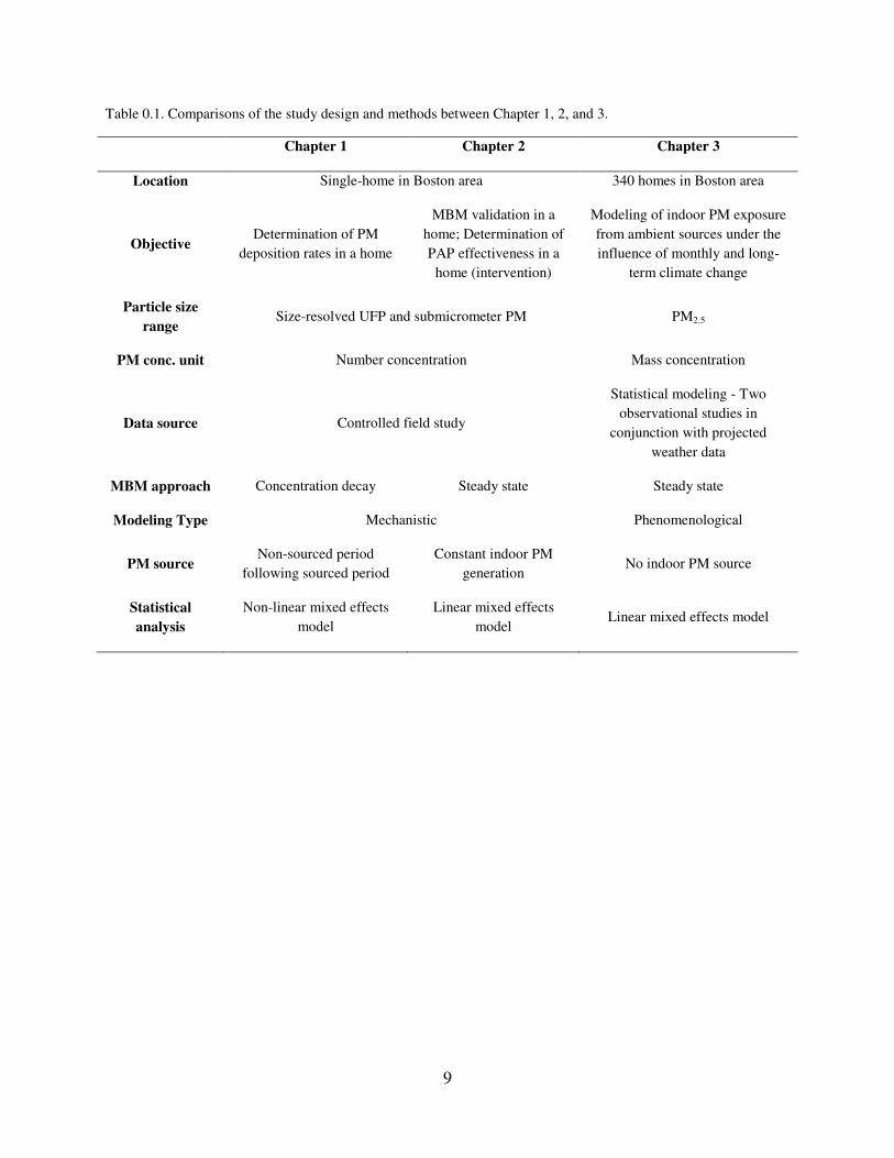
Table 0.1. Comparisons of the study design and methods between Chapter 1, 2, and 3.
Chapter 1 Chapter 2 Chapter 3
Location Single-home in Boston area 340 homes in Boston area
Objective Determination of PM
deposition rates in a home
MBM validation in a
home; Determination of
PAP effectiveness in a
home (intervention)
Modeling of indoor PM exposure
from ambient sources under the
influence of monthly and long-
term climate change
Particle size
range Size-resolved UFP and submicrometer PM PM2.5
PM conc. unit Number concentration Mass concentration
Data source Controlled field study
Statistical modeling - Two
observational studies in
conjunction with projected
weather data
MBM approach Concentration decay Steady state Steady state
Modeling Type Mechanistic Phenomenological
PM source Non-sourced period
following sourced period
Constant indoor PM
generation No indoor PM source
Statistical
analysis
Non-linear mixed effects
model
Linear mixed effects
model Linear mixed effects model
10
Bibliography
(1) Pope, C.; Dockery, D.; Schwartz, J. Review of Epidemiological Evidence of Health-Effects
of Particulate Air-Pollution. Inhal. Toxicol. 1995, 7 (1), 1-18; 10.3109/08958379509014267.
(2) Peters, A.; Dockery, D.; Muller, J.; Mittleman, M. Increased particulate air pollution and the
triggering of myocardial infarction. Circulation 2001, 103 (23), 2810-2815.
(3) Schwartz, J.; Dockery, D.; Neas, L. Is daily mortality associated specifically with fine
particles? J. Air Waste Manage. Assoc. 1996, 46 (10), 927-939.
(4) Klepeis, N.; Nelson, W.; Ott, W.; Robinson, J.; Tsang, A.; Switzer, P.; Behar, J.; Hern, S.;
Engelmann, W. The National Human Activity Pattern Survey (NHAPS): a resource for assessing
exposure to environmental pollutants. J. Expo. Anal. Environ. Epidemiol. 2001, 11 (3), 231-252;
10.1038/sj.jea.7500165.
(5) Liu D. and Nazaroff, W.W. Modeling pollutant penetration across building envelopes.
Atmospheric Environment 2001, 35, 4451-4462.
(6) Hinds, W.C. Aerosol Technology: Properties, Behavior, and Measurement of Airborne
Particles. Wiley: New York, 1999; .
(7) Lai, A.C.K.; Byrne, M.A.; Goddard, A.J.H. Experimental studies of the effect of rough
surfaces and air speed on aerosol deposition in a test chamber. Aerosol Science and Technology
2002, 36 (10), 973-982; 10.1080/02786820290092249.
11
(8) Thatcher, T.L.; Lai, A.C.K.; Moreno-Jackson, R.; Sextro, R.G.; Nazaroff, W.W. Effects of
room furnishings and air speed on particle deposition rates indoors. Atmos. Environ. 2002, 36
(11), 1811-1819; 10.1016/S1352-2310(02)00157-7.
(9) Liu, D. and Nazaroff, W.W. Modeling pollutant penetration across building envelopes.
Atmospheric Environment 2001, , 4451-4462.
(10) Liu, D. and Nazaroff, W.W. Particle Penetration Through Building Cracks. Aerosol Science
and Technology 2003, 37, 565-573.
(11) Chen, C. and Zhao, B. Review of relationship between indoor and outdoor particles: I/O
ratio, infiltration factor and penetration factor. Atmospheric Environment 2011, 45 (2), 275-288.
(12) Wallace, L. Indoor Particles: A Review. J. Air Waste Manage. Assoc. 1996, 46, 98-126.
(13) Barn, P.; Larson, T.; Noullett, M.; Kennedy, S.; Copes, R.; Brauer, M. Infiltration of forest
fire and residential wood smoke: an evaluation of air cleaner effectiveness. Journal of Exposure
Science and Environmental Epidemiology 2008, 18 (5), 503-511.
(14) Wallace, L.A.; Mitchell, H.; T O'Connor, G.; Neas, L.; Lippmann, M.; Kattan, M. Particle
concentrations in inner-city homes of children with asthma: the effect of smoking, cooking, and
outdoor pollution. Environmental health perspectives 2003, 111 (9), 1265.
(15) Wallace, L.A.; Emmerich, S.J.; Howard-Reed, C. Continuous measurements of air change
rates in an occupied house for 1 year: the effect of temperature, wind, fans, and windows.
Journal of exposure analysis and environmental epidemiology 2002, 12 (4), 296-306.
12
(16) Wallace, L. and Williams, R. Use of personal-indoor-outdoor sulfur concentrations to
estimate the infiltration factor and outdoor exposure factor for individual homes and persons.
Environmental science & technology 2005, 39 (6), 1707-1714.
(17) Haghighat, F.; Brohus, H.; Rao, J. Modelling air infiltration due to wind fluctuations—A
review. Building and Environment, 2000, 35 (5), 377-385.
(18) Sarnat, J.A.; Koutrakis, P.; Suh, H.H. Assessing the relationship between personal
particulate and gaseous exposures of senior citizens living in Baltimore, MD. Journal of the Air
& Waste Management Association 2000, 50 (7), 1184-1198.
(19) Howard-Reed, C.; Wallace, L.A.; Emmerich, S.J. Effect of ventilation systems and air
filters on decay rates of particles produced by indoor sources in an occupied townhouse. Atmos.
Environ. 2003, 37 (38), 5295-5306; 10.1016/j.atmosenv.2003.09.012.
(20) Abt, E.; Suh, H.H.; Catalano, P.; Koutrakis, P. Relative contribution of outdoor and indoor
particle sources to indoor concentrations. Environ. Sci. Technol. 2000, 34 (17), 3579-3587;
10.1021/es990348y.
(21) Nazaroff, W.W. Indoor particle dynamics. Indoor air 2004, 14 (s7), 175-183.
(22) Abt, E.; Suh, H.H.; Allen, G.; Koutrakis, P. Characterization of indoor particle sources: A
study conducted in the metropolitan Boston area. Environmental Health Perspectives 2000, 108
(1), 35.
13
(23) Wallace, L.A.; Emmerich, S.J.; Howard-Reed, C. Source strengths of ultrafine and fine
particles due to cooking with a gas stove. Environmental Science & Technology 2004, 38 (8),
2304-2311.
(24) Shaughnessy, R. and Sextro, R. What is an effective portable air cleaning device? A review.
Journal of Occupational and Environmental Hygiene 2006, 3 (4), 169-181;
10.1080/15459620600580129.
(25) Sublett, J.L. Effectiveness of Air Filters and Air Cleaners in Allergic Respiratory Diseases:
A Review of the Recent Literature. Current Allergy and Asthma Reports 2011, 11 (5), 395-402;
10.1007/s11882-011-0208-5.
(26) Waring, M.S.; Siegel, J.A.; Corsi, R.L. Ultrafine particle removal and generation by
portable air cleaners. Atmos. Environ. 2008, 42 (20), 5003-5014;
10.1016/j.atmosenv.2008.02.011.
(27) Sultan, Z.M.; Nilsson, G.J.; Magee, R.J. Removal of ultrafine particles in indoor air:
Performance of various portable air cleaner technologies. Hvac&R Research 2011, 17 (4), 513-
525; 10.1080/10789669.2011.579219.
(28) Offermann, F.; Sextro, R.; Fisk, W.; Grimsrud, D.; Nazaroff, W.; Nero, A.; Revzan, K.;
Yater, J. Control of Respirable Particles in Indoor Air with Portable Air Cleaners. Atmos.
Environ. 1985, 19 (11), 1761-1771; 10.1016/0004-6981(85)90003-4.
14
(29) Shaughnessy, R.; Levetin, E.; Blocker, J.; Subkette, K. Effectiveness of Portable Indoor Air
Cleaners - Sensory Testing Results. Indoor Air-International Journal of Indoor Air Quality and
Climate 1994, 4 (3), 179-188; 10.1111/j.1600-0668.1994.t01-1-00006.x.
(30) Long, C.M.; Suh, H.H.; Catalano, P.J.; Koutrakis, P. Using time- and size-resolved
particulate data to quantify indoor penetration and deposition behavior. Environ. Sci. Technol.
2001, 35 (10), 2089-2099; 10.1021/es001477d.
(31) Hodas, N.; Meng, Q.; Lunden, M.M.; Turpin, B.J. Toward refined estimates of ambient PM
2.5 exposure: Evaluation of a physical outdoor-to-indoor transport model. Atmospheric
Environment, 2014, 83, 229-236.
(32) Sarnat, J.A.; Long, C.M.; Koutrakis, P.; Coull, B.A.; Schwartz, J.; Suh, H.H. Using sulfur
as a tracer of outdoor fine particulate matter. Environmental Science & Technology 2002, 36
(24), 5305-5314.
(33) Chen, C. and Zhao, B. Review of relationship between indoor and outdoor particles: I/O
ratio, infiltration factor and penetration factor. Atmospheric Environment 2011, 45 (2), 275-288.
(34) Wallace, L. and Howard-Reed, C. Continuous monitoring of ultrafine, fine, and coarse
particles in a residence for 18 months in 1999-2000. . Journal of the Air & Waste Management
Association 2002, 52 (7), 828-844.
(35) Kearney, J.; Wallace, L.; MacNeill, M.; Héroux, M.E.; Kindzierski, W.; Wheeler, A.
Residential infiltration of fine and ultrafine particles in Edmonton. Atmospheric Environment
2014, 94, 793-805.

15
(36) Dawson, J.P.; Adams, P.J.; Pandis, S.N. Sensitivity of PM 2.5 to climate in the Eastern US:
a modeling case study. Atmospheric chemistry and physics 2007, 7 (16), 4295-4309.
16
CHAPTER 1
Size-Resolved Deposition Rates for Ultrafine and Submicrometer Particles in a Residential
Housing Unit
Environmental Science & Technology. 2014, 48 (17), 10282–10290
17
Abstract
We estimated the size-resolved particle deposition rates for the ultrafine and submicron particles
using a nonlinear regression method with unknown particle background concentrations during
non-sourced period following a controlled sourced period in a well-mixed residential
environment. A dynamic adjustment method in conjunction with the constant injection of tracer
gas was used to maintain the air exchange rate at three target levels across the range of 0.61-1.24
air change per hour (ACH). Particle deposition was found to be highly size dependent with rates
ranging from 0.68±0.10 to 5.03±0.20 h-1 (mean±s.e). Our findings also suggest that the effect of
air exchange on the particle deposition under enhanced air mixing was relatively small when
compared to both the strong influence of size-dependent deposition mechanisms and the effects
of mechanical air mixing by fans. Nonetheless, the significant association between air exchange
and particle deposition rates for a few size categories indicated potential influence of air
exchange on particle deposition. In the future, the proposed approach can be used to explore the
separate or composite effects between air exchange and air mixing on particle deposition rates,
which will contribute to improved assessment of human exposure to ultrafine and submicron
particles.
Key words: Deposition; Ultrafine particles; Submicron particles; Residential indoor air quality;
Air exchange; Nonlinear regression

18
Introduction
Epidemiological studies have shown association between exposure to ambient fine
particulate matters and adverse health effects such as mortality and onset of cardiovascular
events (1-3). Exposure to indoor fine particles is of particular concern, as people spend more
than 85% of their time in enclosed buildings with the majority of that time in residences (4). An
important parameter in assessing residential particle exposures is indoor particle deposition rate,
a natural removal mechanism that contributes to the reduction of airborne particle levels indoors.
Studies conducted in occupied houses have demonstrated size-specific characteristics for
deposition rates: elevated levels for larger (>1 µm) and ultrafine particles (<100 nm), but
comparatively lower rates for submicron particles (0.1-1.0 µm) (5-11).
Despite the consistent size-dependent trend of the deposition rates, reported values of the
deposition estimates vary by more than an order of magnitude for submicron and ultrafine
particles of similar sizes. Such wide variability could possibly be due to differences in the study
designs and data analysis methods, building characteristics, furnishings, and many other factors.
Although no standard method has been established, most studies adopted the mass balance model
in conjunction with on-site measurements to determine the size-resolved deposition rates in
residential environments and assumed that the air was well-mixed (5, 7-14). However, results
from these studies suggest high uncertainties in the estimated deposition rates, partially due to
limitations in acquiring reliable measurements on particle background concentrations during
tests, potential bias from using average daily air exchange rate to represent real time air exchange
measurements, or difficulty in decoupling the particle deposition rate from another model
parameter (penetration coefficient). As a result, more research is still needed to adequately assess
the size-resolved deposition rates in real-life situations.
19
The deposition rates of submicron and ultrafine particles have been found to be strongly
influenced by indoor air mixing. Factors commonly known to affect indoor air mixing include
mechanical mixing by fans, ventilation, and air exchange between indoor and outdoor
environments. Positive associations between mechanical air mixing and particle deposition rates
have been reported from previous studies during the operation of either portable or central fans
in the ventilation system (8, 10, 15-18). On the other hand, studies conducted in occupied houses
have found inconsistent associations between particle deposition rates and air exchange (8, 11,
19, 20). As the amount of mechanical mixing increases, the consequent increase in air movement
could mask the effect of air exchange on particle deposition rate, especially on closed window
days. However, it remains unclear how much mechanical air mixing is sufficient that the effect
of air exchange becomes negligible.
We expected that achieving well-maintained test conditions in a home would minimize
uncertainties of the estimated size-resolved deposition rates, and allow us to examine the effect
of air exchange rate on the estimated rates under the enhanced mechanical air mixing using
portable fans. We therefore used a modified approach based on the mass balance model to
determine the size-resolved deposition rates. The main features of this approach are: (1) the
achievement of a well-mixed indoor environment using portable fans; (2) the generation of
artificial particles at a constant rate to substantially elevate indoor concentration prior to the
particle decay measurement; (3) the use of a dynamic method to maintain air exchange rates at
constant levels throughout the sampling period; and (4) the use of the NLIN procedure, which
does not require knowledge of the magnitude of the particle background concentration, to
estimate the size-resolved deposition rates along with their uncertainties. The results from this
20
study would provide indications for future application of the revised approach, and can be used
to assess the human exposure to submicron and ultrafine particles in homes.
Materials and methods
This study was conducted in a fully furnished, non-carpeted and occupied concrete floor
apartment unit in Cambridge, Massachusetts, during November 2011. The apartment consists of
two bedrooms, a kitchen, a living room, a bathroom, and a hallway that connects the living room
and kitchen. There was no air conditioning system in the apartment, and heating was provided by
hydronic radiant heating system. Ventilation in the house depended on the opening of windows,
doors and two small vents that exhausted the air from indoors. These openings remained closed
and taped throughout all sampling periods (with minor adjustments on the taping to maintain
constant air exchange rates). Our study design based on the mass balance approach required the
air in the room to be well-mixed. And after a series of preliminary tests, we selected the kitchen,
living room, and the hallway as the study area (approximately 34.8 m2) to ensure a well-mixed
condition using portable fans. The fans were all at their highest speed settings and were placed in
the same location and orientation for all the tests. No significant indoor sources were present
except for the artificial particle generation system. The layout of the instruments and devices in
the apartment unit is shown in Figure S1.1 in Supporting Information (SI).
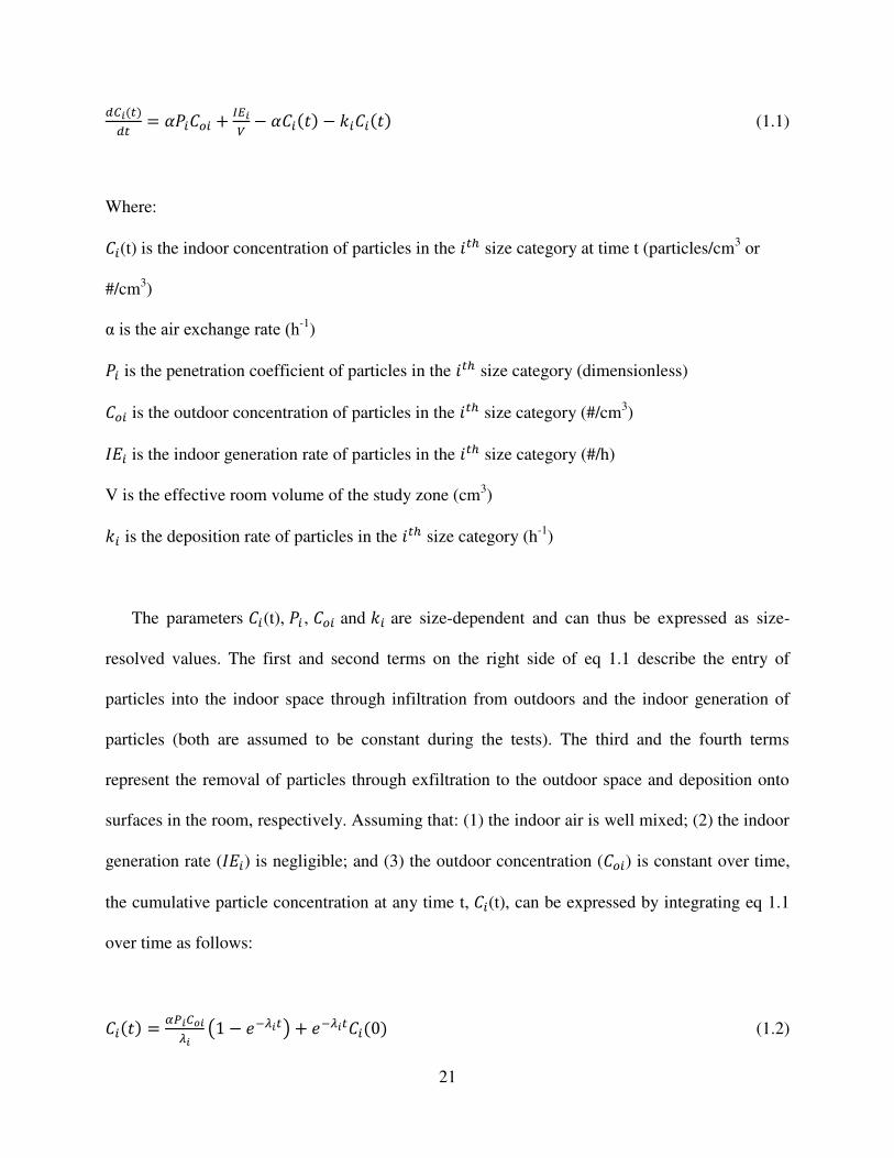
Model description. We used the mass balance approach to model the concentrations of particles
in an indoor space over time. A general form of the model is
21
鳥寵日岫痛岻鳥痛 噺 糠鶏沈系墜沈 髪 彫帳日蝶 伐 糠系沈岫建岻 伐 倦沈系沈岫建岻 (1.1)
Where: 系沈(t) is the indoor concentration of particles in the 件痛朕 size category at time t (particles/cm3 or
#/cm3)
g is the air exchange rate (h-1) 鶏沈 is the penetration coefficient of particles in the 件痛朕 size category (dimensionless) 系墜沈 is the outdoor concentration of particles in the 件痛朕 size category (#/cm3) 荊継沈 is the indoor generation rate of particles in the 件痛朕 size category (#/h)
V is the effective room volume of the study zone (cm3) 倦沈 is the deposition rate of particles in the 件痛朕 size category (h-1)
The parameters 系沈(t), 鶏沈 , 系墜沈 and 倦沈 are size-dependent and can thus be expressed as size-
resolved values. The first and second terms on the right side of eq 1.1 describe the entry of
particles into the indoor space through infiltration from outdoors and the indoor generation of
particles (both are assumed to be constant during the tests). The third and the fourth terms
represent the removal of particles through exfiltration to the outdoor space and deposition onto
surfaces in the room, respectively. Assuming that: (1) the indoor air is well mixed; (2) the indoor
generation rate (荊継沈) is negligible; and (3) the outdoor concentration (系墜沈) is constant over time,
the cumulative particle concentration at any time t, 系沈(t), can be expressed by integrating eq 1.1
over time as follows:
系沈岫建岻 噺 底牒日寵任日碇日 盤な 伐 結貸碇日痛匪 髪 結貸碇日痛系沈岫ど岻 (1.2)
22
Where: 膏沈 噺 糠 髪 倦沈 (1.3) 系沈(0) is the initial concentration at the start of measurement for particles in the 件痛朕 size category
(#/cm3)
eq 1.2 shows that the observed decrease in particle concentration during the decay period is
due to the combination of air exchange between indoors and outdoors and the deposition of
particles onto surfaces within the indoor space. It was employed as the final model in this study
where 系沈岫建岻 and 糠 were measured independently after the generation of artificial particles was
stopped. The measured parameters were subsequently used to determine 倦沈 in the data analysis
phase.
Measurement and adjustment of air exchange rate. The two features involving the air
exchange component required by the model were to maintain a constant 糠 for each test to meet
the model assumption and to determine the actual rate.
Three target air exchange rates (A) were set to determine the size-resolved particle deposition
rates with repeated tests: A=0.60, 0.90, and 1.20 ACH. To achieve this, we applied the sulfur
hexafluoride (SF6) tracer gas method and measured SF6 in two consecutive phases: (1) the
steady-state phase where we used the real-time measurement of steady-state SF6 concentration as
a proxy of 糠, and (2) the exponential decay phase where 糠 was determined (Figure S1.2 in SI)
(21). The former required a constant injection rate of SF6 ( 芸聴庁展 ), under which the SF6
concentration in the room would reach 95% of its steady state (系鎚鎚) in about 3/g hours when 糠
was held constant. The steady-state relationship between the parameters is shown in eq 1.4 (21):
23
系鎚鎚岫喧喧兼岻 噺 町縄鈍展盤陳典ゲ朕貼迭匪底岫朕貼迭岻蝶岫陳典岻 抜 など滞岫喧喧兼岻 (1.4)
At steady state, change in 系鎚鎚 directly reflected the variability of 糠 when 芸聴庁展 and V were
both fixed values. Under this circumstance, we could maintain 糠 by monitoring 系鎚鎚 and adjusting
it to a constant level. In practice, an SF6 generation system was set up to provide a constant
injection rate of 54.20 罰 0.57 cm3/min (mean±s.d.). The SF6 concentration was measured
continuously in the kitchen and living room by two SF6 monitors (Brüel & Kjær model 1302).
For most of the experiments the differences between the SF6 steady state concentrations in
the living room and the kitchen at any time were less than 10%. Prior to the SF6 release, we
closed all the windows, doors and vents and partially sealed the gaps around these closed
openings with masking tape to establish the initial air exchange conditions. When the windows
were closed during the tests, the air exchange in the home was mainly driven by the pressure and
temperature differences between indoor and outdoor environments, leading to infiltration and
exfiltration of air through gaps of doors and windows. The initially established 糠 was adjusted
downward from the highest air exchange condition by partially sealing the gaps with masking
tape to achieve the target level.
Due to the rapid mixing inside of the house, the SF6 steady state concentration reflected the
drift in 糠 within 1 or 2 measurements (about 1 or 2 minutes). To shorten the time to achieve
steady state, a “blast” of SF6 was released over a short period to elevate the SF6 concentration
close to the target steady state level before starting the injection of SF6 at a constant rate. The SF6
24
concentration would then approach 系鎚鎚 which corresponded to a specific 糠 at that time. By
adjusting the sealing of the gaps with masking tape throughout the sampling day, we were able to
keep 系鎚鎚 within 5% of the target value for the specific ACH required based on the relationship in
eq 1.4.
At the end of each sampling day, we stopped the SF6 generation and continued to measure
the SF6 concentration which then followed an exponential decay over time. The decay constant,
which represented 糠 over the decay period, corresponded to 系鎚鎚 of the sampling day and was
determined by fitting a simple linear regression curve between log-transformed SF6
concentration and time (21). We determined the daily average 糠 based on the relationship
between 糠 from the end-of-the-day measurements and the 系鎚鎚 using data from both the nine test
days and the preliminary tests (n=4), given the calculated arithmetic mean of the determined V
(撃博 噺 ひぱ 兼戴, n=13).
Generation and measurement of particles. The High-output Extended Aerosol Respiratory
Therapy (HEART®) nebulizers (Westmed, Inc., Tucson, Arizona) were used to aerosolize
aqueous sodium chloride (NaCl) solution (0.0375% by mass) to generate NaCl particles. To
achieve sufficiently high concentrations for the decay tests, nebulizers that generated aerosols
with comparable rates and size distributions were selected and used in single, double and triple
combinations to achieve similar steady state particle concentrations for each of the three target
air exchange rates. These combinations were tested in the laboratory and had NaCl aerosolization
rates of 16.58±0.32, 32.29±0.98, and 46.24±0.58 g/h for one, two and three nebulizers,
respectively.
25
The TSI Model 3936 scanning mobility particle sizer (SMPS) equipped with a Model 3785
Water-based Condensation Particle Counter (WCPC) was used to measure particles between
0.015 to 0.533 µm (mobility diameter) for size distribution and count concentrations over
consecutive 5-min intervals.
Sampling plan. Steady state particle concentration indoors was achieved in about 2 hours
(“sourced period”), after which we turned off the particle generation system and monitored
particle concentration at consecutive 5-min intervals over approximately one hour of particle
decay (“non-sourced period”). This decay period provided a sufficient number of measurements
for an adequate analysis of the size-resolved particle deposition rates. In total, there were nine
test days with measurements under three target air exchange rates in triplicate (one test per day).
An example of the simultaneous measurements of the total particle and the SF6 concentrations
throughout the test day is depicted in Figure S1.2 in SI.
Data analysis. Particle data were divided into 11 size categories: <25, 25-35, 35-45, 45-55, 55-
65, 65-80, 80-100, 100-150, 150-200, 200-300, and >300 nm. Additionally, total particle
concentrations were also used in the analysis. We estimated 倦沈 based on eq 1.2 using
measurements from the non-sourced period subsequent to the sourced period, which provided
sufficiently high initial concentration prior to decay, 系沈岫ど岻 . The non-sourced period was
carefully defined based on the actual time that we shut off the particle generation system. In the
data analysis phase, 系沈岫ど岻 was assumed to be unknown and allowed to vary around the measured
value to minimize the effect of instrument uncertainty. Similarly, 鶏沈系墜沈 and 倦沈 were treated as
unknown parameters with values greater than zero. The nonlinear approximation procedure,
26
PROC NLIN (SAS Inc. Cary, NC), was used to determine the values of the unknown parameters
(鶏沈系墜沈, 倦沈 and 系沈岫ど岻) through an iterative process to find the best combination of the parameters
which yielded the minimum value of the residual sum of squares (the sum of the squared
differences between the modeled and measured 系沈岫建岻). One important feature of the NLIN
procedure is the selection of “good” starting values for the unknown parameters to prevent the
approximation process from converging to local minima. In this study, multiple starting points
were introduced in the NLIN procedure by specifying their physically feasible ranges with
investigator-defined intervals for each unknown parameter: 100-5,000 by 500 (particles/cm3) for 鶏沈系墜沈 , 0.1-6 by 1 (h-1) for 倦沈 , and 10-5,000 by 100 (particles/cm3) for 系沈岫ど岻. More detailed
description of the procedure can be found in the SI.
Based on the air exchange rate, 倦沈 were determined by the NLIN procedure at three levels:
(1) 倦沈┸底 as 倦沈 for each test, (2) 倦沈┸凋 as the average 倦沈 by the three target air exchange rates
(A=0.60, 0.90 and 1.20 ACH), and (3) 倦沈┸銚鎮鎮 as the average 倦沈 across all the nine tests (Figure
S1.3 in SI). Analysis at the first level was to determine 倦沈 for each test day separately so we
could examine the goodness of fit of the predicted indoor particle concentrations from the NLIN
procedure versus the measured values. This visual examination was necessary because the r-
squared value is generally not a meaningful measure in nonlinear regression analysis. The second
level was used to evaluate the effect of air exchange on the deposition estimates while the third
was to summarize the estimates in comparison with those from the previous studies. In the
analyses for the last two levels, 鶏沈系墜沈 and 系沈岫ど岻 were allowed to have different constant values
for each test day to account for the daily variation of particle concentrations both outdoors and
indoors, while 倦沈 was assumed to be constant under each target air exchange rate for 倦沈┸凋 and
27
constant across all ACH for 倦沈┸銚鎮鎮. Uncertainties for the estimates from the NLIN procedure were
reported as standard errors.
To evaluate the effect of air exchange rate on 倦沈, the estimates determined from the second
level (倦沈┸凋退待┻滞待, 倦沈┸凋退待┻苔待, 倦沈┸凋退怠┻態待) were first examined using a global F test with a significance
level of 0.05 for each particle size category, to see whether the 倦沈 from at least one target ACH
were different from the 倦沈 from the others. Subsequently, pairwise comparisons (n=3) of the 倦沈┸凋
values were made with the level of significance of 0.0167. The F statistics used for the pairwise
comparison procedure were based on the paired data, except that we used the same mean squared
error (MSE) from the global test. By doing so, we were able to make three comparisons on the
same basis (using the same denominator for the F-statistics), and the higher degrees of freedom
from the MSE would contribute to more stable results in the analysis.
Results
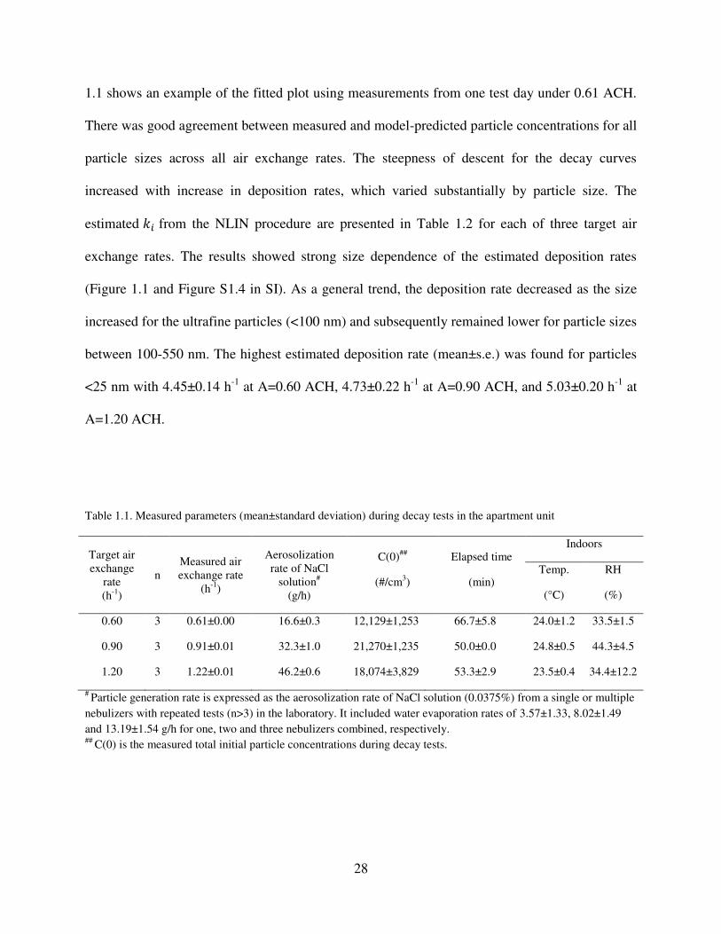
Measured parameters. The measured parameters and indoor conditions in the apartment for the
three target air exchange rates are shown in Table 1.1. The relative humidity (RH) was below the
deliquescence point of NaCl of 75.3% (at 25°C); thus, the particle-associated water was expected
to evaporate completely, leaving cubic crystals of NaCl as the aerosol (22). The variability of
indoor temperature and RH across the test days was small with coefficients of variation of less
than 5%, except for the RH at A=0.90 ACH (coefficient of variation = 10.16%).
Estimated size-resolved deposition rate. Comparisons between the measured particle
concentrations by particle size versus time and the fitted (predicted) values from the NLIN
procedure were made for all nine test days to evaluate the goodness of fit of the model. Figure
28
1.1 shows an example of the fitted plot using measurements from one test day under 0.61 ACH.
There was good agreement between measured and model-predicted particle concentrations for all
particle sizes across all air exchange rates. The steepness of descent for the decay curves
increased with increase in deposition rates, which varied substantially by particle size. The
estimated 倦沈 from the NLIN procedure are presented in Table 1.2 for each of three target air
exchange rates. The results showed strong size dependence of the estimated deposition rates
(Figure 1.1 and Figure S1.4 in SI). As a general trend, the deposition rate decreased as the size
increased for the ultrafine particles (<100 nm) and subsequently remained lower for particle sizes
between 100-550 nm. The highest estimated deposition rate (mean±s.e.) was found for particles
<25 nm with 4.45±0.14 h-1 at A=0.60 ACH, 4.73±0.22 h-1 at A=0.90 ACH, and 5.03±0.20 h-1 at
A=1.20 ACH.
Table 1.1. Measured parameters (mean±standard deviation) during decay tests in the apartment unit
Target air exchange
rate (h-1)
n Measured air exchange rate
(h-1)
Aerosolization rate of NaCl
solution# (g/h)
C(0)##
(#/cm3)
Elapsed time
(min)
Indoors
Temp.
(°C)
RH
(%)
0.60 3 0.61±0.00 16.6±0.3 12,129±1,253 66.7±5.8 24.0±1.2 33.5±1.5
0.90 3 0.91±0.01 32.3±1.0 21,270±1,235 50.0±0.0 24.8±0.5 44.3±4.5
1.20 3 1.22±0.01 46.2±0.6 18,074±3,829 53.3±2.9 23.5±0.4 34.4±12.2
# Particle generation rate is expressed as the aerosolization rate of NaCl solution (0.0375%) from a single or multiple
nebulizers with repeated tests (n>3) in the laboratory. It included water evaporation rates of 3.57±1.33, 8.02±1.49
and 13.19±1.54 g/h for one, two and three nebulizers combined, respectively. ## C(0) is the measured total initial particle concentrations during decay tests.
29
Effect of air exchange rate under enhanced air mixing. In general, estimates of 倦沈 at A=1.20
ACH (倦沈┸凋退怠┻態待岻 were lower than those from the other two target air exchange rates, except for
the smallest and the largest particle size categories (Table 1.2). Results from the pairwise
comparisons showed no statistically significant differences between 倦沈┸凋退待┻滞待 and 倦沈┸凋退待┻苔待 for
particles of all sizes (Table S1.1 in SI). Nevertheless, significant differences were observed in a
few size categories between the highest target air exchange rate (A=1.20 ACH) and the other two
lower target ACH. Specifically, 倦沈┸凋退怠┻態待 values were significantly lower than 倦沈┸凋退待┻苔待 for
particles of 35-45 nm, 65-80 nm and 80-100 nm. A similar trend was shown between 倦沈┸凋退怠┻態待
and 倦沈┸凋退待┻滞待 for particles of 35-45 nm, 80-100 nm and 150-200 nm. Overall, given the enhanced
air mixing conditions, our findings have only found sporadic statistically significant differences,
but not a consistent and relatively meaningful trend in the effect of air exchange rate on
deposition rate across all particle sizes.
30
Figure 1.1. Comparison of the predicted and measured particle concentrations during the decay
periods for the 11 particle size categories, using data from one sampling day (0.61 ACH) as an
example. The solid markers represent the actual measurements while the solid lines are the
predicted decay curves from the NLIN procedure.
31
Table 1.2. Estimated deposition rate by particle size, categorized based on the midpoint of mobility diameter (dm).
Target air exchange rate
(h-1)
Particle size
(nm) n
Estimated 倦沈 (h-
1)
Approx. s.e.#
(h-1)
Approx. 95% C.I.##
Lower Upper
0.60
<25 42 4.45 0.14 4.16 4.74
25-35 42 3.33 0.07 3.18 3.47
35-45 42 2.61 0.06 2.48 2.73
45-55 42 2.13 0.08 1.97 2.29
55-65 42 1.82 0.07 1.67 1.96
65-80 42 1.45 0.07 1.32 1.59
80-100 42 1.40 0.09 1.21 1.58
100-150 42 1.13 0.09 0.96 1.30
150-200 42 1.12 0.11 0.89 1.36
200-300 42 1.13 0.13 0.87 1.39
>300 41 1.11 0.17 0.77 1.46
Total### 42 2.23 0.05 2.14 2.33
0.90
<25 32 4.73 0.22 4.28 5.17
25-35 32 3.36 0.11 3.14 3.57
35-45 32 2.59 0.08 2.42 2.75
45-55 32 2.05 0.08 1.88 2.21
55-65 32 1.80 0.07 1.66 1.94
65-80 32 1.62 0.06 1.50 1.74
80-100 32 1.37 0.08 1.21 1.54
100-150 32 1.00 0.06 0.87 1.12
150-200 32 1.01 0.11 0.78 1.24
200-300 32 0.95 0.16 0.62 1.27
>300 32 1.03 0.26 0.49 1.56
Total### 32 2.30 0.05 2.19 2.41
32
(Table 1.2 continued)
1.20
<25 34 5.03 0.20 4.61 5.44
25-35 34 3.25 0.12 3.00 3.50
35-45 34 2.25 0.09 2.07 2.43
45-55 34 1.83 0.12 1.58 2.09
55-65 34 1.51 0.12 1.25 1.76
65-80 34 1.24 0.09 1.05 1.43
80-100 34 0.96 0.11 0.75 1.18
100-150 34 0.96 0.10 0.76 1.16
150-200 34 0.68 0.10 0.46 0.89
200-300 34 0.91 0.14 0.62 1.20
>300 34 1.42 0.24 0.94 1.91
Total### 34 2.06 0.06 1.93 2.19
# Approx. s.e. is the approximate standard error of the estimated 倦沈 from the NLIN procedure. ## Approx. 95% C.I. is the approximate 95% confidence interval for the estimated 倦沈 from the NLIN procedure. ### It represents the total particle concentration which is the sum of size-resolved particle concentrations.
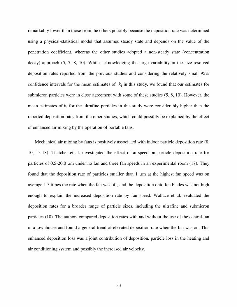
Discussion
The estimated particle deposition rates in this study were found to be strongly dependent on
size, as suggested by previous studies (5, 7, 8, 10). The partially V-shaped curve of deposition
rate by size is due to the size-dependent deposition mechanisms where ultrafine particles are
removed by indoor surfaces due to diffusion while submicron particles are too large to diffuse
and too small to settle effectively by gravitation (23, 24). As the size increases for submicron
particles, gravitation gradually becomes a more dominant mechanism for deposition.
Comparisons of size-resolved particle deposition rates for particles less than 1 µm in
occupied houses are depicted in Figure 1.2. The numeric values of 倦沈┸銚鎮鎮 used for comparison can
be found in Table S1.2 in SI. The size-resolved deposition rates presented by Long et al. were
33
remarkably lower than those from the others possibly because the deposition rate was determined
using a physical-statistical model that assumes steady state and depends on the value of the
penetration coefficient, whereas the other studies adopted a non-steady state (concentration
decay) approach (5, 7, 8, 10). While acknowledging the large variability in the size-resolved
deposition rates reported from the previous studies and considering the relatively small 95%
confidence intervals for the mean estimates of 倦沈 in this study, we found that our estimates for
submicron particles were in close agreement with some of these studies (5, 8, 10). However, the
mean estimates of 倦沈 for the ultrafine particles in this study were considerably higher than the
reported deposition rates from the other studies, which could possibly be explained by the effect
of enhanced air mixing by the operation of portable fans.
Mechanical air mixing by fans is positively associated with indoor particle deposition rate (8,
10, 15-18). Thatcher et al. investigated the effect of airspeed on particle deposition rate for
particles of 0.5-20.0 µm under no fan and three fan speeds in an experimental room (17). They
found that the deposition rate of particles smaller than 1 µm at the highest fan speed was on
average 1.5 times the rate when the fan was off, and the deposition onto fan blades was not high
enough to explain the increased deposition rate by fan speed. Wallace et al. evaluated the
deposition rates for a broader range of particle sizes, including the ultrafine and submicron
particles (10). The authors compared deposition rates with and without the use of the central fan
in a townhouse and found a general trend of elevated deposition rate when the fan was on. This
enhanced deposition loss was a joint contribution of deposition, particle loss in the heating and
air conditioning system and possibly the increased air velocity.
34
Figure 1.2. Comparison of deposition rates of particles less than 1 µm in occupied houses
between previous and the current studies (5, 7, 8, 10). The shaded area represents the 95%
confidence interval for the estimated mean deposition rate by particle size in this study.
35
When provided air mixing, the particles are brought from the bulk air to the boundary layer
near the indoor surfaces via advection, through which they deposit onto the surfaces by diffusion
(24). The use of central or portable fans thus leads to a substantial increase in the amount of air
mixing indoors and contributes to increased particle deposition rates by facilitating the transport
of particles to the boundary layer and by reducing the thickness of the boundary layer (24, 25).
Such influence was more pronounced for ultrafine particles where diffusion is the dominant
mechanism for deposition. Since the level of mechanical air mixing in the current study was
thought to be much stronger than that in the other studies, the boundary layer processes explain
largely why our deposition estimates are higher, especially for ultrafine particles.
Air exchange rate is an important factor in determining particle deposition rate not only
because it is a parameter in the mass balance model but also for its relation to indoor air mixing.
Increase in air exchange rate can result in increased particle deposition by facilitating indoor air
movement while it has the parallel effect of lowering the residence time of particles indoors.
However, evaluation of these effects can be challenging, especially when complicated by
mechanical air mixing that is positively associated with particle deposition rate. Previous studies
conducted in occupied houses have shown large disparities in the effect of air exchange on
deposition rate (8, 11, 19, 20). Nevertheless, evaluations of the different findings were difficult
to do due to the varying ranges of air exchange rates along with their corresponding ventilation
or air mixing conditions. Rim et al. investigated the functional relationship between air exchange
and particle deposition for ultrafine particles based on two different levels of air mixing in an
uninhabited test house (18). They discovered that the difference in the deposition rates due to air
mixing by central fan became smaller when the air exchange rate increased (from all windows
closed to 2 windows open 7.5 cm each). Compared to Rim et al., the small effect of air exchange
36
rate on size-resolved particle deposition rates in the present study could be explained by the
masking effect of mechanical air mixing over the relatively narrow range of natural air exchange
in the apartment on closed window days (18). However, it remains unclear to what extent the
variation in one factor would mask the effect from the other.
In this study, we also estimated the average particle deposition rates based on integrated
measurements in the attempt to allow comparison with previous studies that used integrated
measurements (Table 1.2). Table 1.3 presents a summary of the experimental conditions for the
selected home studies which estimated size-resolved or integrated particle deposition rates for
particles smaller than 1 µm. The wide variability of estimates across studies could be attributed
not only to differences in chemical and physical characteristics of particles, interiors of the
houses (e.g., furnishing), use of air cleaners or air furnaces, ventilation system, surface-to-
volume ratios, indoor air mixing levels, air exchange rate, occupancy, but also to differences in
experimental and analytical methods. The integrated particle deposition rates in our study ranged
from 2.06±0.06 to 2.30±0.05 h-1 across the three target air exchange rates and were comparable
with findings from the others (13, 14). Overall, smaller uncertainties were observed in this study
for both of the size-resolved and the integrated estimates largely due to well-maintained
experimental conditions.
High indoor particle concentrations have been reported to result in coagulation which was
considered as an important mechanism of particle loss indoors, especially for ultrafine particles
(24, 26). Rim et al. investigated the coagulation of ultrafine particles during indoor episodes
resulting from various indoor sources and concluded that coagulation should be accounted for
when the number concentration for ultrafine particles exceeds 20,000 particles/cm3 (26). In this
study, the total particle number concentrations at the steady state from which the decay started
37
were approximately 20,000 particles/cm3 under various test conditions and was no more than
10% higher than this threshold for all sampling days. Therefore, the influence of coagulation on
the estimated deposition rate was considered to be negligible.
One strength of the NLIN procedure is that measurement of particle background
concentration (shown as 底牒日寵任日碇日 in eq 1.2) during each decay period is not required to determine
the particle deposition rate. Instead, the unknown value of 鶏沈系墜沈 can be estimated simultaneously
in the same procedure (Figure S1.5 in SI). In an attempt to see how deposition estimates might
have differed had we adopted the commonly used linear regression method without knowing the
particle background concentrations, we conducted analysis using the same data but with iterated
background values to estimate 倦沈 by fitting a simple linear regression curve between log-
transformed 系沈岫建岻 and time. Estimates of 倦沈 from the linear regression model showed wide
variability across different background values; however, only slight variation was observed in
the corresponding r-squared values. As an extreme example, ignoring the background (底牒日寵任日碇日 噺ど) could lead to underestimation of deposition rate over a factor of 2 or more. It also resulted in
negative estimates of 倦沈 for particles >100 nm at 1.21 ACH, indicating that the accuracy of these
estimates was questionable. Our analysis suggests that three potential concerns can rise from the
linear regression method when the background level is unknown: (1) estimates of 倦沈 can be
increasingly sensitive to the variation in the background level as the sampling duration increases;
(2) neglecting the background concentration typically results in the underestimation of 倦沈; and
(3) using r-squared value as a criterion for best estimates of 倦沈 can lead to inaccuracies, as slight
changes in the r-squared value correspond to a wide range of values of estimated 倦沈. Given these
38
concerns, the nonlinear regression approach was considered to be more reliable than the linear
regression approach for this study.
Table 1.3. Experimental characteristics from selected studies on deposition rates for particles of less than 1µm in
houses (5, 8-10, 12-14).
Study House type Main
particle source
Particle size
range (µm)##
Sample type
Mixing mechanism
Particle monitor#
Air exchange
rate (h-1)
Deposition rate for <1 µm (h-1)
Abt et al.
(2000)
4 homes (occupied)
Cooking 0.02-
10 Size-
resolved Natural
convection SMPS, APS
0.16- 0.66
0.02- 1.70
Long et al.
(2001)
9 nonsmoking
homes (occupied)
Ambient 0.02-
10 Size-
resolved Natural
convection SMPS, APS
0.89 (winter);
2.1 (summer)
0.004-0.35 (winter)
0.15-0.59 (summer)
Chao et al.
(2003)
6 homes (occupied)
Ambient 0.02-9.65
Integrated, Size-
resolved
Natural convection
P-Trak, APS
1.28± 0.54
0.27 (APS) 0.52
(P-Trak) Howard-Reed et
al. (2003)
A townhouse (occupied)
Cooking, candle,
kitty litter
0.30-10
Size-resolved
Central fan (on/off)
OPC 0.64± 0.56###
0.29-0.47 (fan off) 0.66-1.0 (fan on)
Wallace et al.
(2004)
A townhouse (occupied)
Cooking, candle,
kitty litter
0.011-5.43
Size-resolved
Central fan (on/off)
SMPS, APS, OPC
0.64± 0.56
0.70-4.10 (fan off) 0.90-3.92 (fan on)
Kearney et al.
(2011)
94 homes (occupied)
Ambient 0.02-1.0
Integrated Various
types P-Trak
0.12- 0.37
(inter-quatile)
####
0.68- 0.87
Stephens and
Siegel (2012)
18 homes (unoccupied)
Ambient 0.02-1.0
Integrated
Central fan plus two box fans
(on)
P-Trak 0.13- 0.95
(GM)*
0.31- 3.24
Wallace et al.
(2013)
74 homes (occupied)
Cooking 0.02-1.0,
PM2.5 Integrated
Various types
P-Trak, DustTrak
0.35± 0.30
1.17± 0.94
This study (2013)
A home (occupied)
NaCl nebuli-zation
0.015-0.533
Size-resolved
Portable fans (on)
SMPS 0.61- 1.24
0.68- 5.03
# SMPS: scanning mobility particle sizer; APS: aerodynamic particle sizer; OPC: optical particle counter. ## Particles measured by SMPS were reported with mobility diameter. APS measured particles based on aerodynamic diameter, while OPS measured particles by light-scattering. ### The values were reported by He et al.11. #### The study was conducted in one winter and two summer seasons.* GM=geometric mean.
39
One of the limitations of this study is the lack of a standard method to validate the accuracy
of the estimates from the NLIN procedure because there is no standard method to determine size-
resolved particle deposition rate. Generally, applications of the nonlinear approach in estimating
particle deposition rates in residential environment have reportedly suffered from issues such as
low confidence in decoupling the unknown parameters and high uncertainties in the estimates of
the parameters which arise from different study designs (12, 19, 27). In comparison, the
measurements for the current study were taken in a well-mixed environment with well-fit
exponential decay curves under nearly constant air exchange rates, which was expected to
generate more reliable results. The estimated 系沈岫ど岻 was highly comparable to the actual
measurement with differences within 10% for all the analyses. Furthermore, the estimates of 倦沈 returned from the NLIN procedure were within tight 95% confidence intervals, indicating low
uncertainties in the mean deposition rates. Higher uncertainties were observed for particles larger
than 300 nm, possibly due to fewer particle numbers in this size category. The uncertainties,
when expressed as standard deviation over the mean, were highly comparable to those estimated
by Rim et al. in a manufactured test house using a technique equivalent to the NLIN procedure
(20). Consequently, the present study design in conjunction with the nonlinear analytical
approach was regarded as adequate to generate robust estimates of 倦沈. Another limitation of this study is the consequent enhanced air mixing condition from
operating a number of portable fans in the apartment, which is rare in real life situations during
closed-window days. The extent of the fan-driven air mixing in the apartment was expected to
exceed the mixing level from the central fan operation in the previous studies, leading to elevated
levels of 倦沈 (8, 10). As the level of mechanical air mixing increases to a certain extent, it can
mask the effect of air exchange rate, as suggested by the results in the current study. Therefore,
40
caution should be taken when generalizing the findings from this study to predict particle
deposition rates in normal housing conditions. However, the use of fans to facilitate air mixing
helped achieve a well-mixed environment and brought about several advantages. First, it fulfilled
the requirements of the two mass balance models which we used to determine g and 倦沈 ,
respectively, and made it possible to maintain constant air exchange rates. Second, it reduced the
uncertainty in the estimation of 倦沈 from the NLIN procedure because particle concentration
decay followed the mass balance model more closely when the particles are uniformly
distributed indoors, which in turn led to better fitting of the model to the data. It is noteworthy
that the use of the NLIN procedure also helped relieve the constraint of making assumptions on
the particle background levels indoors during data analysis, especially when the outdoor particle
concentrations were unavailable. Third, it allowed us to evaluate the effect of air exchange rate
on 倦沈 as well as the relative level of particle deposition by particle size when provided the same
amount of air mixing indoors. Last but not least, the enhanced deposition loss due to reinforced
air mixing would contribute to higher reduction of human exposures, especially to ultrafine and
submicron particles. Nevertheless, more conservative rates (lower values) should be considered
for exposure assessment in homes without significant air mixing.
The study design in conjunction with the NLIN procedure provided a feasible and alternative
method for estimating particle deposition rates when the background concentration cannot be
measured (assuming that the background concentration is relatively constant over the sampling
period). The same approach can further be applied to understand other particle behaviors in the
future. For example, it can be used to determine simultaneously the size-resolved particle
deposition rates and penetration coefficients when given the measured outdoor concentrations. In
addition, this approach can be used to study the effect of air exchange on particle deposition

41
under varying levels of air mixing by adjusting fans at different speeds. The understanding of
both the particle deposition and penetration rates in a typical home and the factors affecting them
contributes to improved assessment and prediction of human exposure to particles. Subsequent
precautionary measures or actions of intervention can then be taken to reduce particle exposure
in homes.
42
Bibliography
(1) Pope, C.; Thun, M.; Namboodiri, M.; Dockery, D.; Evans, J.; Speizer, F.; Heath, C.
Particulate Air-Pollution as a Predictor of Mortality in a Prospective-Study of Us Adults.
American Journal of Respiratory and Critical Care Medicine 1995, 151 (3), 669-674.
(2) Schwartz, J.; Dockery, D.; Neas, L. Is daily mortality associated specifically with fine
particles? J. Air Waste Manage. Assoc. 1996, 46 (10), 927-939.
(3) Peters, A.; Dockery, D.; Muller, J.; Mittleman, M. Increased particulate air pollution and the
triggering of myocardial infarction. Circulation 2001, 103 (23), 2810-2815.
(4) Klepeis, N.; Nelson, W.; Ott, W.; Robinson, J.; Tsang, A.; Switzer, P.; Behar, J.; Hern, S.;
Engelmann, W. The National Human Activity Pattern Survey (NHAPS): a resource for assessing
exposure to environmental pollutants. J. Expo. Anal. Environ. Epidemiol. 2001, 11 (3), 231-252;
10.1038/sj.jea.7500165.
(5) Abt, E.; Suh, H.H.; Catalano, P.; Koutrakis, P. Relative contribution of outdoor and indoor
particle sources to indoor concentrations. Environ. Sci. Technol. 2000, 34 (17), 3579-3587;
10.1021/es990348y.
(6) Vette, A.F.; Rea, A.W.; Lawless, P.A.; Rodes, C.E.; Evans, G.; Highsmith, V.R.; Sheldon, L.
Characterization of indoor-outdoor aerosol concentration relationships during the Fresno PM
exposure studies. Aerosol Science and Technology 2001, 34 (1), 118-126;
10.1080/027868201300082120.
43
(7) Long, C.M.; Suh, H.H.; Catalano, P.J.; Koutrakis, P. Using time- and size-resolved
particulate data to quantify indoor penetration and deposition behavior. Environ. Sci. Technol.
2001, 35 (10), 2089-2099; 10.1021/es001477d.
(8) Howard-Reed, C.; Wallace, L.A.; Emmerich, S.J. Effect of ventilation systems and air filters
on decay rates of particles produced by indoor sources in an occupied townhouse. Atmos.
Environ. 2003, 37 (38), 5295-5306; 10.1016/j.atmosenv.2003.09.012.
(9) Chao, C.; Wan, M.; Cheng, E. Penetration coefficient and deposition rate as a function of
particle size in non-smoking naturally ventilated residences. Atmos. Environ. 2003, 37 (30),
4233-4241; 10.1016/S1352-2310(03)00560-0.
(10) Wallace, L.A.; Emmerich, S.J.; Howard-Reed, C. Effect of central fans and in-duct filters on
deposition rates of ultrafine and fine particles in an occupied townhouse. Atmos. Environ. 2004,
38 (3), 405-413; 10.1016/j.atmosenv.2003.10.003.
(11) He, C.R.; Morawska, L.; Gilbert, D. Particle deposition rates in residential houses. Atmos.
Environ. 2005, 39 (21), 3891-3899; 10.1016/j.atmosenv.2005.03.016.
(12) Kearney, J.; Wallace, L.; MacNeill, M.; Xu, X.; VanRyswyk, K.; You, H.; Kulka, R.;
Wheeler, A.J. Residential indoor and outdoor ultrafine particles in Windsor, Ontario. Atmos.
Environ. 2011, 45 (40), 7583-7593; 10.1016/j.atmosenv.2010.11.002.
(13) Stephens, B. and Siegel, J.A. Penetration of ambient submicron particles into single-family
residences and associations with building characteristics. Indoor Air 2012, 22 (6), 501-513;
10.1111/j.1600-0668.2012.00779.x.
44
(14) Wallace, L.; Kindzierski, W.; Kearney, J.; MacNeill, M.; Heroux, M.; Wheeler, A.J. Fine
and Ultrafine Particle Decay Rates in Multiple Homes. Environ. Sci. Technol. 2013, 47 (22),
12929-12937; 10.1021/es4025809t.
(15) Mosley, R.B.; Greenwell, D.J.; Sparks, L.E.; Guo, Z.; Tucker, W.G.; Fortmann, R.;
Whitfield, C. Penetration of ambient fine particles into the indoor environment. Aerosol Science
and Technology 2001, 34 (1), 127-136; 10.1080/02786820117449.
(16) Lai, A.C.K.; Byrne, M.A.; Goddard, A.J.H. Experimental studies of the effect of rough
surfaces and air speed on aerosol deposition in a test chamber. Aerosol Science and Technology
2002, 36 (10), 973-982; 10.1080/02786820290092249.
(17) Thatcher, T.L.; Lai, A.C.K.; Moreno-Jackson, R.; Sextro, R.G.; Nazaroff, W.W. Effects of
room furnishings and air speed on particle deposition rates indoors. Atmos. Environ. 2002, 36
(11), 1811-1819; 10.1016/S1352-2310(02)00157-7.
(18) Rim, D.; Wallace, L.A.; Persily, A.K. Indoor Ultrafine Particles of Outdoor Origin:
Importance of Window Opening Area and Fan Operation Condition. Environ. Sci. Technol.
2013, 47 (4), 1922-1929; 10.1021/es303613e.
(19) Allen, R.; Larson, T.; Sheppard, L.; Wallace, L.; Liu, L. Use of real-time light scattering
data to estimate the contribution of infiltrated and indoor-generated particles to indoor air.
Environ. Sci. Technol. 2003, 37 (16), 3484-3492; 10.1021/es021007e.
(20) Rim, D.; Wallace, L.; Persily, A. Infiltration of Outdoor Ultrafine Panicles into a Test
House. Environ. Sci. Technol. 2010, 44 (15), 5908-5913; 10.1021/es101202a.
45
(21) ASTM Standard Test Method for Determining Air Change in a Single Zone by Means of a
Tracer Gas Dilution. E741-00. American Society for Testing and Materials International: West
Conshohocken, Pennsylvania, 2001; .
(22) Tang, I. and Munkelwitz, H. Composition and Temperature-Dependence of the
Deliquescence Properties of Hygroscopic Aerosols. Atmospheric Environment Part A-General
Topics 1993, 27 (4), 467-473; 10.1016/0960-1686(93)90204-C.
(23) Hinds, W.C. Aerosol Technology: Properties, Behavior, and Measurement of Airborne
Particles. Wiley: New York, 1999; .
(24) Nazaroff, W.W. Indoor particle dynamics. Indoor Air 2004, 14, 175-183; 10.1111/j.1600-
0668.2004.00286.x.
(25) Lai, A.C.K. and Nazaroff, W.W. Modeling indoor particle deposition from turbulent flow
onto smooth surfaces. J. Aerosol Sci. 2000, 31 (4), 463-476.
(26) Rim, D.; Green, M.; Wallace, L.; Persily, A.; Choi, J. Evolution of Ultrafine Particle Size
Distributions Following Indoor Episodic Releases: Relative Importance of Coagulation,
Deposition and Ventilation. Aerosol. Sci. Technol. 2012, 46 (5), 494-503;
10.1080/02786826.2011.639317.
(27) Bennett, D. and Koutrakis, P. Determining the infiltration of outdoor particles in the indoor
environment using a dynamic model. J. Aerosol Sci. 2006, 37 (6), 766-785;
10.1016/j.jaerosci.2005.05.020.
46
Supporting information (SI)
NLIN procedure for data analysis. PROC NLIN is a well-established procedure in SAS. It
utilizes an iterative process to estimate the specified unknown parameters which in this study are 鶏沈系墜沈, 倦沈 and 系沈岫ど岻. The procedure starts from initially guessed values (starting values) for the
parameters and subsequently searches for the best solution (combination of parameter values)
that yields the minimum value of the residual sum of squares. In theory, there can be multiple
solutions that give rise to convergence to end the procedure. However, the solutions might not
always be meaningful or close to the actual values. For example, if the procedure starts from
initially guessed values that are far from the actual values, it could converge to a local minimum
and result in biased estimates. To prevent this situation from occurring, we set 鶏沈系墜沈, 倦沈 and 系沈岫ど岻 to be greater than zero because the particle concentrations and deposition rates should
theoretically be positive values. Additionally, we specified the ranges and the intervals to allow
multiple starting values for all three parameters so that the NLIN procedure could determine the
best combination of the starting values. In fact, the NLN procedure converged to the same
estimated values even without using multiple starting values for 鶏沈系墜沈, 倦沈 and 系沈岫ど岻. This was
most likely due to the distinct profiles of the decay curves which contributed to more robust
estimation in this study.
In the analysis, we treated 系沈岫ど岻 as an unknown parameter instead of using the actual
measurements. The major reason for that was because the determination of 倦沈 from the decay
curve was sensitive to the initial concentration. We therefore specified it as an unknown
parameter and allowed the NLIN procedure to estimate its value based on the data. This
approach was advantageous in three aspects. First, we minimized the influence of the instrument
47
uncertainty for more robust 倦沈 estimation by not using the actual measurements, given that 倦沈 was sensitive to 系沈岫ど岻 . Secondly, we could still compare the estimated values from NLIN
procedure to the actual measurements to check for consistency. Thirdly, consistency between the
estimated and measured 系沈岫ど岻 indicated reliable estimation for 鶏沈系墜沈 and 倦沈 because all three
parameters were approximated simultaneously in the same procedure.
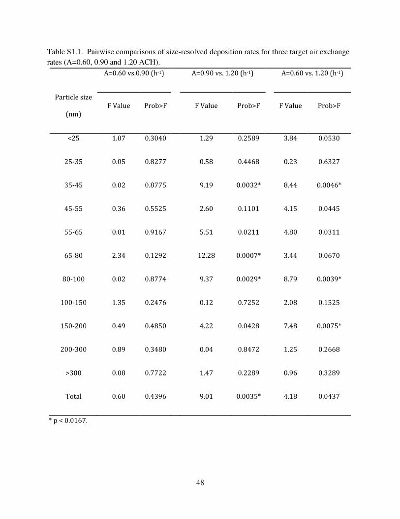
48
Table S1.1. Pairwise comparisons of size-resolved deposition rates for three target air exchange
rates (A=0.60, 0.90 and 1.20 ACH).
A=0.60 vs.0.90 (h-1)
A=0.90 vs. 1.20 (h-1)
A=0.60 vs. 1.20 (h-1)
Particle size
(nm)
F Value Prob>F
F Value Prob>F
F Value Prob>F
<25 1.07 0.3040
1.29 0.2589
3.84 0.0530
25-35 0.05 0.8277
0.58 0.4468
0.23 0.6327
35-45 0.02 0.8775
9.19 0.0032*
8.44 0.0046*
45-55 0.36 0.5525
2.60 0.1101
4.15 0.0445
55-65 0.01 0.9167
5.51 0.0211
4.80 0.0311
65-80 2.34 0.1292
12.28 0.0007*
3.44 0.0670
80-100 0.02 0.8774
9.37 0.0029*
8.79 0.0039*
100-150 1.35 0.2476
0.12 0.7252
2.08 0.1525
150-200 0.49 0.4850
4.22 0.0428
7.48 0.0075*
200-300 0.89 0.3480
0.04 0.8472
1.25 0.2668
>300 0.08 0.7722
1.47 0.2289
0.96 0.3289
Total 0.60 0.4396
9.01 0.0035*
4.18 0.0437
* p < 0.0167.
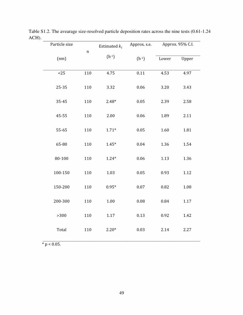
49
Table S1.2. The avearage size-resolved particle deposition rates across the nine tests (0.61-1.24
ACH).
Particle size
(nm)
n
Estimated 倦沈
(h-1)
Approx. s.e.
(h-1)
Approx. 95% C.I.
Lower Upper
<25 110 4.75 0.11 4.53 4.97
25-35 110 3.32 0.06 3.20 3.43
35-45 110 2.48* 0.05 2.39 2.58
45-55 110 2.00 0.06 1.89 2.11
55-65 110 1.71* 0.05 1.60 1.81
65-80 110 1.45* 0.04 1.36 1.54
80-100 110 1.24* 0.06 1.13 1.36
100-150 110 1.03 0.05 0.93 1.12
150-200 110 0.95* 0.07 0.82 1.08
200-300 110 1.00 0.08 0.84 1.17
>300 110 1.17 0.13 0.92 1.42
Total 110 2.20* 0.03 2.14 2.27
* p < 0.05.
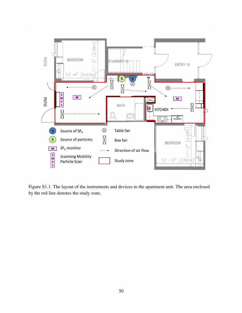
50
Figure S1.1. The layout of the instruments and devices in the apartment unit. The area enclosed
by the red line denotes the study zone.
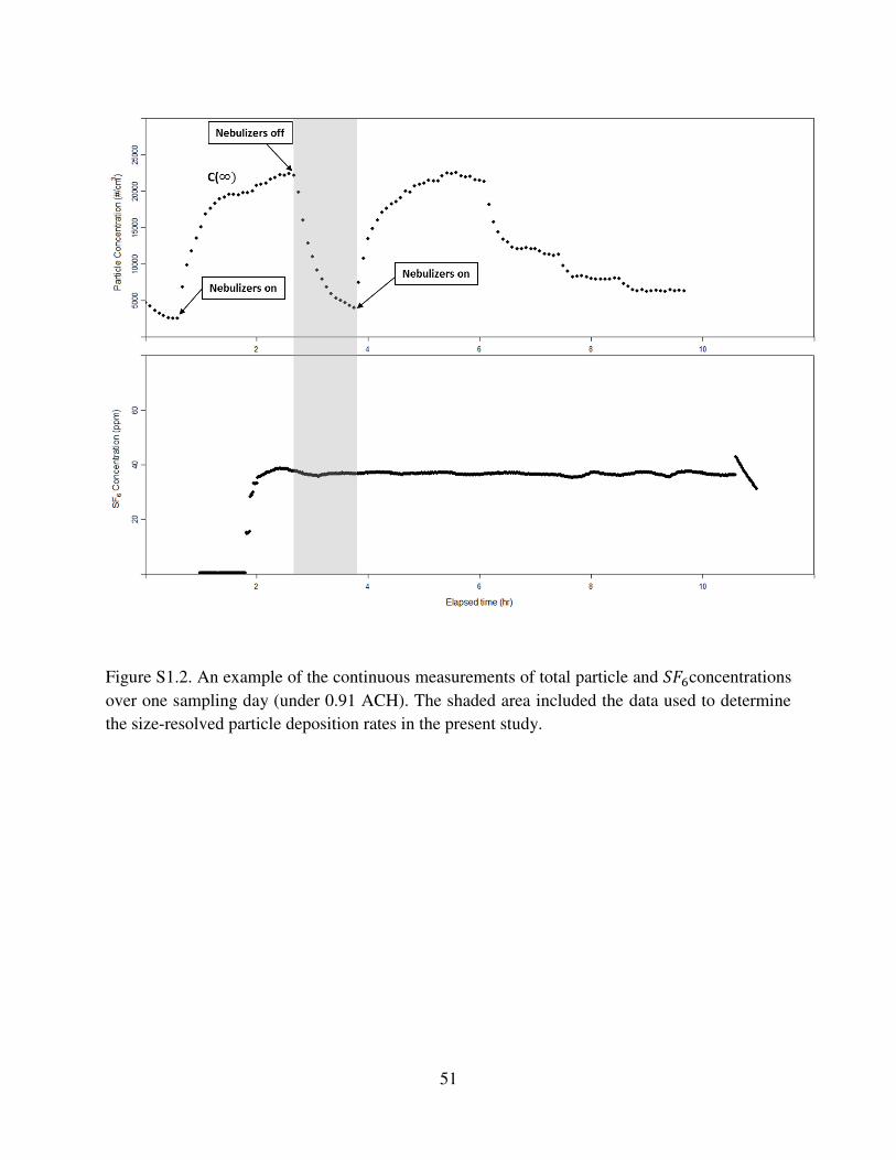
51
Figure S1.2. An example of the continuous measurements of total particle and 鯨繋滞concentrations
over one sampling day (under 0.91 ACH). The shaded area included the data used to determine
the size-resolved particle deposition rates in the present study.
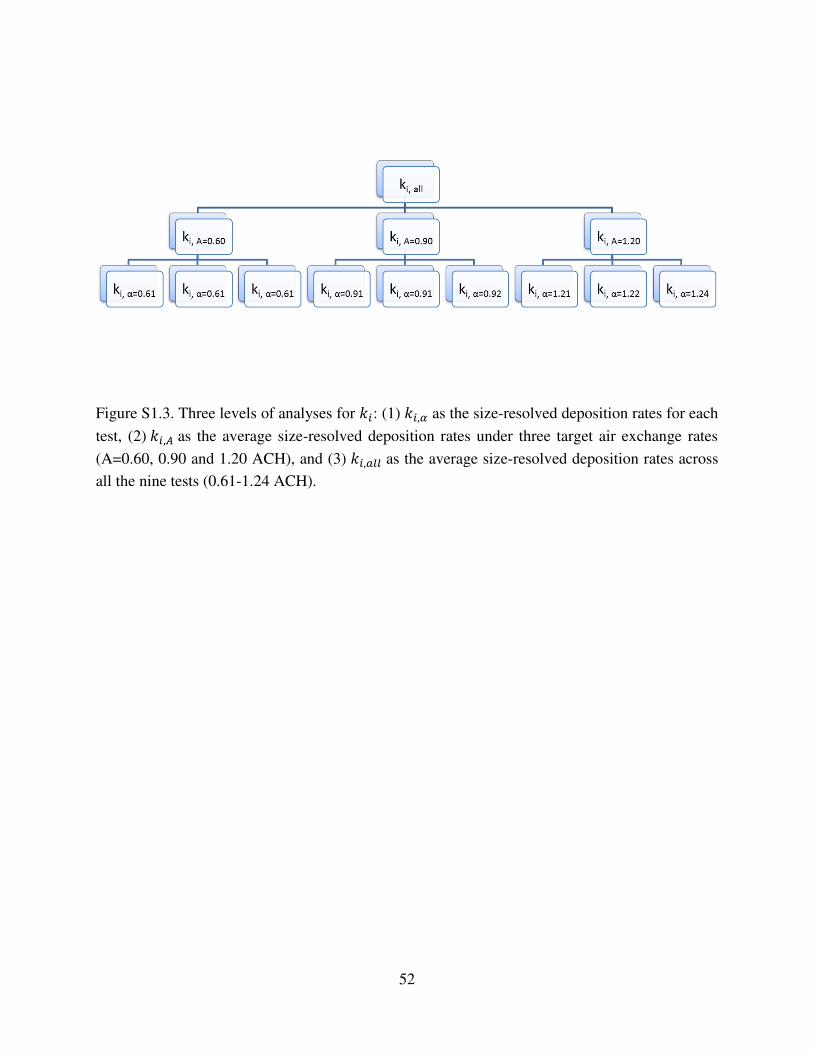
52
Figure S1.3. Three levels of analyses for 倦沈: (1) 倦沈┸底 as the size-resolved deposition rates for each
test, (2) 倦沈┸凋 as the average size-resolved deposition rates under three target air exchange rates
(A=0.60, 0.90 and 1.20 ACH), and (3) 倦沈┸銚鎮鎮 as the average size-resolved deposition rates across
all the nine tests (0.61-1.24 ACH).
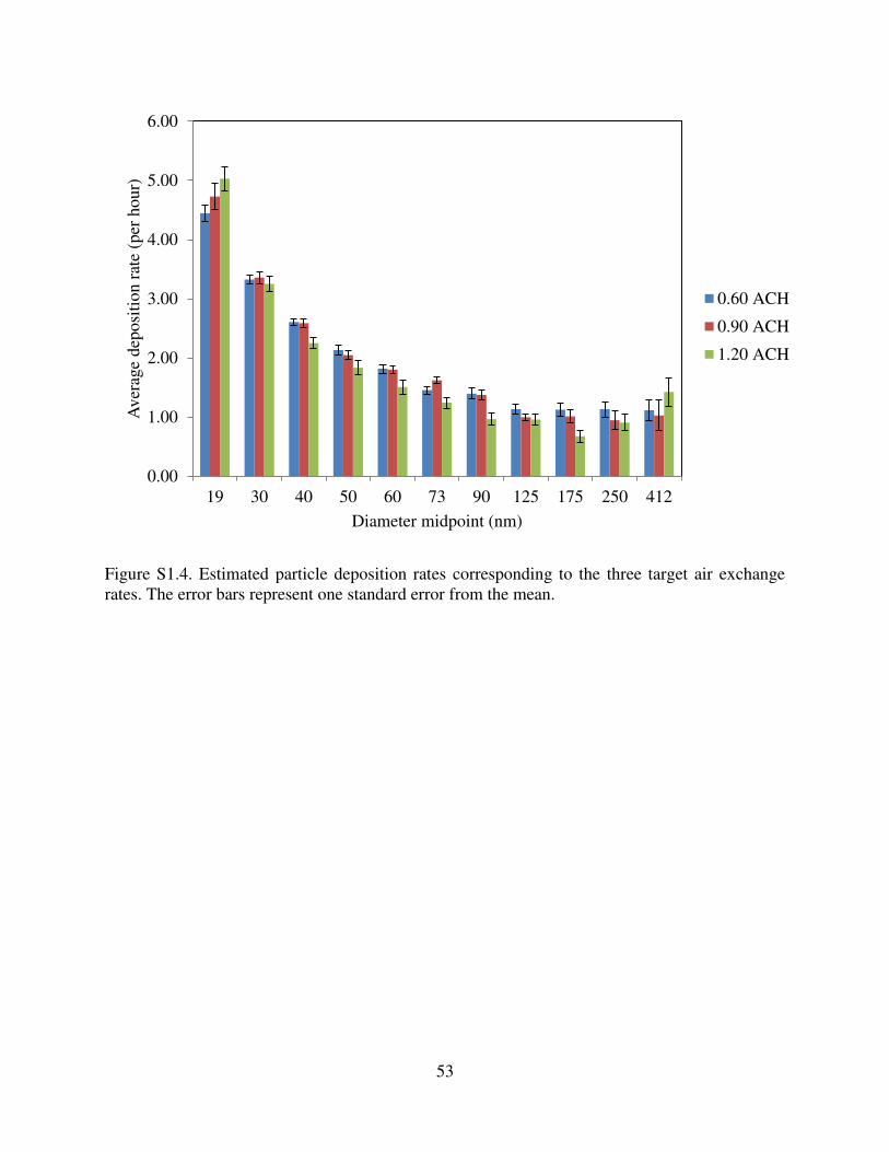
53
Figure S1.4. Estimated particle deposition rates corresponding to the three target air exchange rates. The error bars represent one standard error from the mean.
0.00
1.00
2.00
3.00
4.00
5.00
6.00
19 30 40 50 60 73 90 125 175 250 412
Ave
rage
dep
osit
ion
rate
(pe
r ho
ur)
Diameter midpoint (nm)
0.60 ACH
0.90 ACH
1.20 ACH
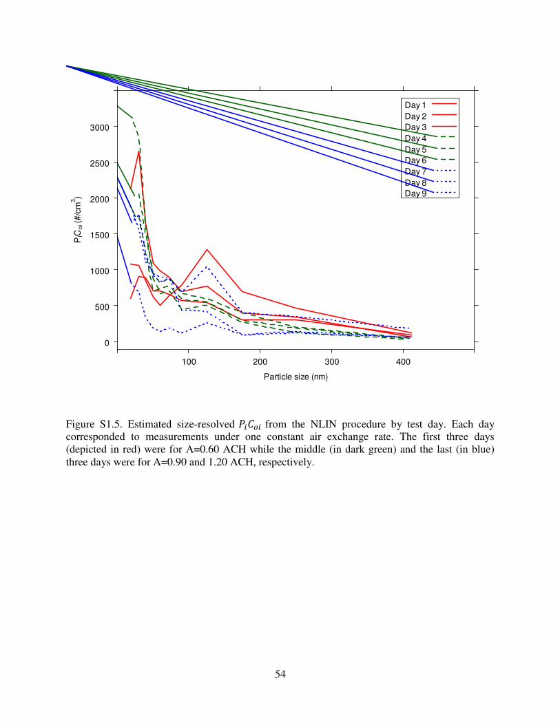
54
Figure S1.5. Estimated size-resolved 鶏沈系墜沈 from the NLIN procedure by test day. Each day corresponded to measurements under one constant air exchange rate. The first three days (depicted in red) were for A=0.60 ACH while the middle (in dark green) and the last (in blue) three days were for A=0.90 and 1.20 ACH, respectively.
Particle size (nm)
PiC
oi (
#/c
m3)
0
500
1000
1500
2000
2500
3000
100 200 300 400
Day 1
Day 2
Day 3
Day 4
Day 5
Day 6
Day 7
Day 8
Day 9
55
CHAPTER 2
Validation and Application of the Mass Balance Model to Determine the Effectiveness of
Portable Air Purifiers in Removing Ultrafine and Submicrometer Particles in an
Apartment
Environmental Science & Techonology. (Published online on July 24th, 2015)
56
Abstract
We validated the use of the mass balance model to determine the effectiveness of portable air
purifiers in removing ultrafine (<0.10 µm) and submicrometer particles (0.10-0.53 µm) in an
apartment. We evaluated two identical portable air purifiers, equipped with high efficiency
particulate air filters, for their performance under three different air flow settings and three target
air exchange rates: 0.60, 0.90 and 1.20 h-1. We subsequently used a mixed effects model to
estimate the slope between the measured and modeled effectiveness by particle size. Our study
showed that effectiveness was highly particle size-dependent. For example, at the lowest target
air exchange rate, it ranged from 0.33 to 0.56, 0.51 to 0.75, and 0.60 to 0.81 for the three air
purifier flow settings, respectively. Our findings suggested that filtration was the dominant
removal mechanism for submicrometer particles, whereas deposition could play a more
important role in ultrafine particle removal. We found reasonable agreement between measured
and modeled effectiveness with size-resolved slopes ranging from 1.11±0.06 to 1.25±0.07
(mean±s.e.), except for particles <35 nm. Our study design can be applied to investigate the
performances of other portable air purifiers as well as the influences of various parameters on
effectiveness in different residential settings.
Key words: Portable air purifier; Mass balance model; Size-resolved effectiveness; Ultrafine
particles; Submicrometer particles; Residential indoor air quality
57
Introduction
There is compelling evidence of the association between exposure to ambient fine particulate
matter (<2.5 µm) and adverse health effects, such as heart disease and mortality (1-3). People
spend the majority of their time indoors (4), where ambient fine particles penetrate and
contribute to the indoor particle level along with particles generated through cooking and other
indoor activities (5-7). A potentially effective way to remove fine particles indoors is to use
portable air purifiers (PAPs), especially in homes without in-duct filtration systems (8-10).
The effectiveness of PAPs has been defined as the proportion of particles they remove in the
indoor environment (9). It can be determined either by direct measurements of indoor particle
concentrations with and without the use of PAP(s), or by model predictions with known model
parameter values. The latter method is often conducted using the mass balance model (MBM),
where effectiveness can be expressed as a function of the Clean Air Delivery Rate (CADR). The
CADR is a metric that denotes the clean air that a PAP provides based on different particle sizes
and can be expressed as the product of the flow rate and the filtration efficiency of the portable
device (9, 11). Chamber studies have shown that PAPs equipped with high-efficiency particulate
air (HEPA) filters have the highest CADRs compared to many other PAP cleaning technologies
(12-14).
The highest modeled effectiveness for PAPs equipped with HEPA filters reported from
previous studies ranged from 0.60 to 0.95 (14-17). However, the accuracy of these values is
unknown, due to the lack of quantitative validation of the modeled results with empirical data in
a residential setting. For example, some studies have set the CADR values in scenarios that
assumed the PAP(s) were 100% efficient in removing particles of all sizes, neglecting air bypass
58
and short-circuiting situations that decrease CADRs (15). Others have predicted the effectiveness
using experimentally measured CADRs, but cited values from separate studies for the other
model parameters that were determined under different experimental conditions from each other
(14, 16, 17).
The overall objective of this study was to more comprehensively assess the effectiveness of
PAP(s) equipped with HEPA filters in removing ultrafine particles (UFPs) (<0.1 µm) and
submicrometer particles (0.10-0.53 µm) in an apartment, based on the commonly used mass
balance approach with the support of empirical data. Our four specific aims were to: (1)
experimentally determine the size-resolved PAP effectiveness using directly measured particle
concentrations with and without the operation of PAPs; (2) model and predict the size-resolved
effectiveness using individually measured model input parameters during the same test periods
as the first aim; (3) compare the modeled and experimentally-determined effectiveness values by
particle size; and (4) examine the effect of particle size, air exchange and PAP flow rate on PAP
effectiveness. To minimize measurement uncertainty, we conducted the study under well-
maintained test conditions in the apartment. We expect our findings to provide information on
the reliability of the MBM predictions, which contribute to more accurate assessment of the
reduction of residents’ exposure to indoor fine particles due to the use of PAP.
Materials and methods
This study was conducted in a fully furnished, non-carpeted and occupied concrete floor
apartment unit in Cambridge, Massachusetts, during November 2011. The selected study area,
including the living room and the kitchen connected with a hallway, is approximately 34.8 m2.
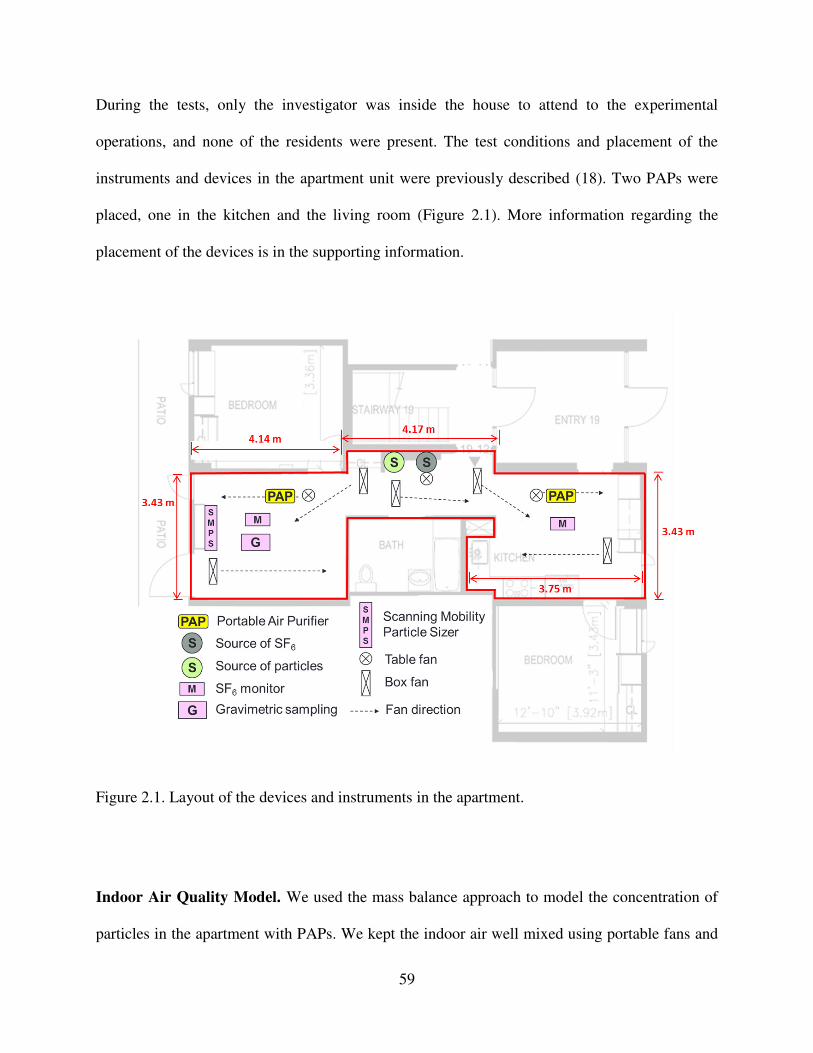
59
During the tests, only the investigator was inside the house to attend to the experimental
operations, and none of the residents were present. The test conditions and placement of the
instruments and devices in the apartment unit were previously described (18). Two PAPs were
placed, one in the kitchen and the living room (Figure 2.1). More information regarding the
placement of the devices is in the supporting information.
Figure 2.1. Layout of the devices and instruments in the apartment.
Indoor Air Quality Model. We used the mass balance approach to model the concentration of
particles in the apartment with PAPs. We kept the indoor air well mixed using portable fans and
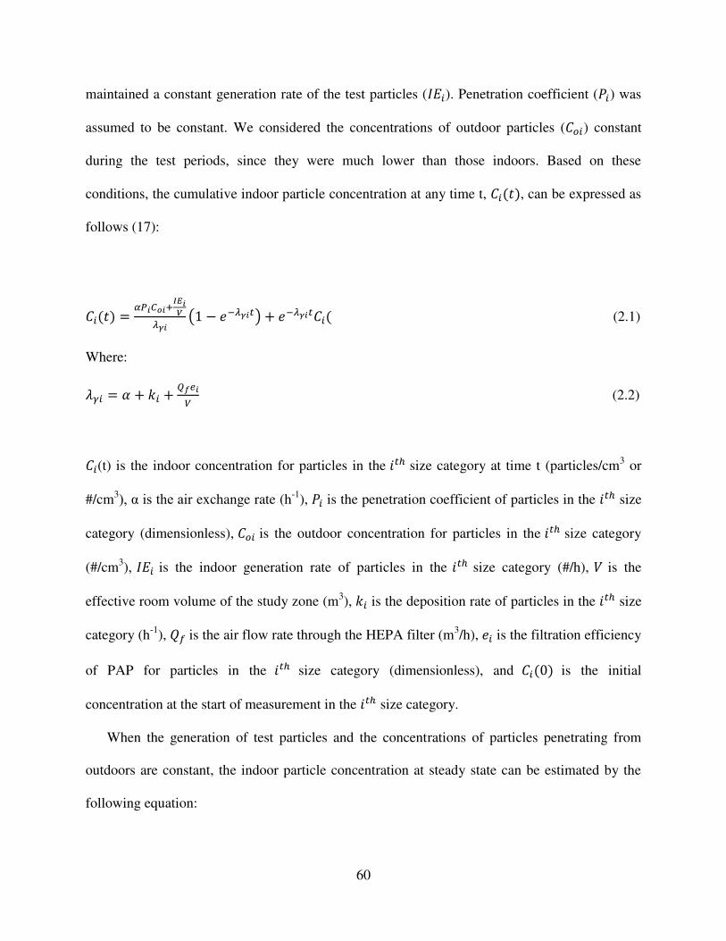
60
maintained a constant generation rate of the test particles (荊継沈). Penetration coefficient (鶏沈) was
assumed to be constant. We considered the concentrations of outdoor particles (系墜沈) constant
during the test periods, since they were much lower than those indoors. Based on these
conditions, the cumulative indoor particle concentration at any time t, 系沈岫建岻, can be expressed as
follows (17):
系沈岫建岻 噺 底牒日寵任日袋内曇日楠碇婆日 盤な 伐 結貸碇婆日痛匪 髪 結貸碇婆日痛系沈岫 (2.1)
Where: 膏廷沈 噺 糠 髪 倦沈 髪 町肉勅日蝶 (2.2)
系沈(t) is the indoor concentration for particles in the 件痛朕 size category at time t (particles/cm3 or
#/cm3), g is the air exchange rate (h-1), 鶏沈 is the penetration coefficient of particles in the 件痛朕 size
category (dimensionless), 系墜沈 is the outdoor concentration for particles in the 件痛朕 size category
(#/cm3), 荊継沈 is the indoor generation rate of particles in the 件痛朕 size category (#/h), 撃 is the
effective room volume of the study zone (m3), 倦沈 is the deposition rate of particles in the 件痛朕 size
category (h-1), 芸捗 is the air flow rate through the HEPA filter (m3/h), 結沈 is the filtration efficiency
of PAP for particles in the 件痛朕 size category (dimensionless), and 系沈岫ど岻 is the initial
concentration at the start of measurement in the 件痛朕 size category.
When the generation of test particles and the concentrations of particles penetrating from
outdoors are constant, the indoor particle concentration at steady state can be estimated by the
following equation:
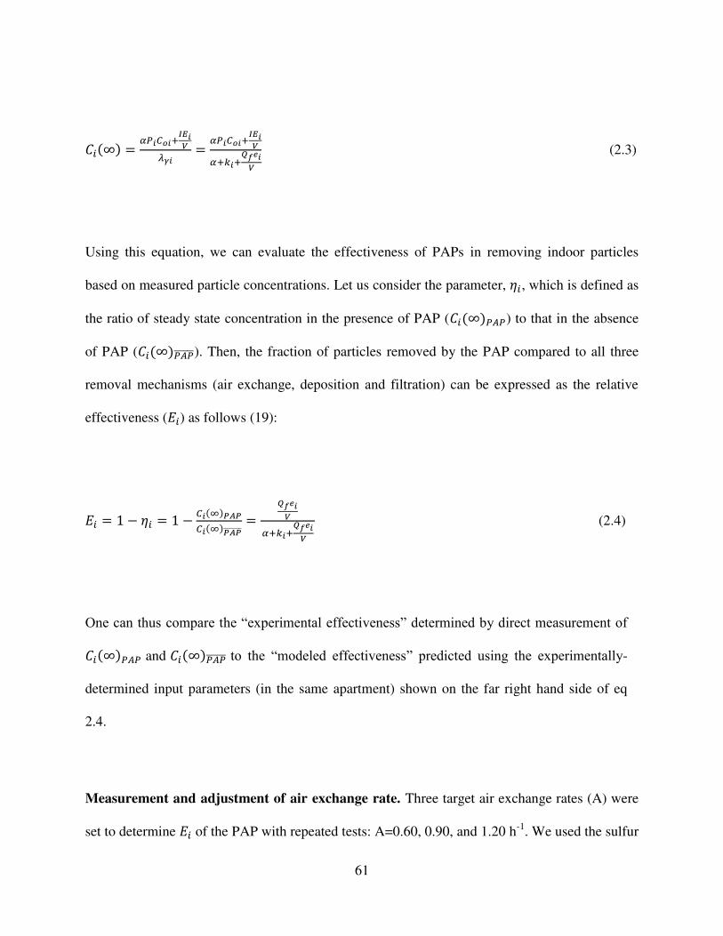
61
系沈岫タ岻 噺 底牒日寵任日袋内曇日楠碇婆日 噺 底牒日寵任日袋内曇日楠底袋賃日袋楢肉賑日楠 (2.3)
Using this equation, we can evaluate the effectiveness of PAPs in removing indoor particles
based on measured particle concentrations. Let us consider the parameter, 考沈, which is defined as
the ratio of steady state concentration in the presence of PAP (系沈岫タ岻牒凋牒) to that in the absence
of PAP (系沈岫タ岻牒凋牒博博博博博博). Then, the fraction of particles removed by the PAP compared to all three
removal mechanisms (air exchange, deposition and filtration) can be expressed as the relative
effectiveness (継沈) as follows (19):
継沈 噺 な 伐 考沈 噺 な 伐 寵日岫著岻鍋豚鍋寵日岫著岻鍋豚鍋博博博博博博博 噺 楢肉賑日楠底袋賃日袋楢肉賑日楠 (2.4)
One can thus compare the “experimental effectiveness” determined by direct measurement of 系沈岫タ岻牒凋牒 and 系沈岫タ岻牒凋牒博博博博博博 to the “modeled effectiveness” predicted using the experimentally-
determined input parameters (in the same apartment) shown on the far right hand side of eq
2.4.
Measurement and adjustment of air exchange rate. Three target air exchange rates (A) were
set to determine 継沈 of the PAP with repeated tests: A=0.60, 0.90, and 1.20 h-1. We used the sulfur
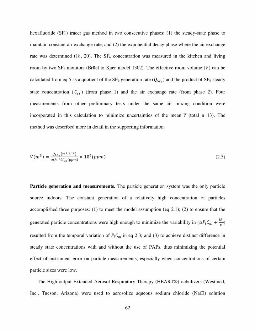
62
hexafluoride (SF6) tracer gas method in two consecutive phases: (1) the steady-state phase to
maintain constant air exchange rate, and (2) the exponential decay phase where the air exchange
rate was determined (18, 20). The SF6 concentration was measured in the kitchen and living
room by two SF6 monitors (Brüel & Kjær model 1302). The effective room volume (撃) can be
calculated from eq 5 as a quotient of the SF6 generation rate (芸聴庁展) and the product of SF6 steady
state concentration ( 系鎚鎚 ) (from phase 1) and the air exchange rate (from phase 2). Four
measurements from other preliminary tests under the same air mixing condition were
incorporated in this calculation to minimize uncertainties of the mean 撃 (total n=13). The
method was described more in detail in the supporting information.
撃岫兼戴岻 噺 町縄鈍展盤陳典ゲ朕貼迭匪底岫朕貼迭岻寵濡濡岫椎椎陳岻 抜 など滞岫喧喧兼岻 (2.5)
Particle generation and measurements. The particle generation system was the only particle
source indoors. The constant generation of a relatively high concentration of particles
accomplished three purposes: (1) to meet the model assumption (eq 2.1); (2) to ensure that the
generated particle concentrations were high enough to minimize the variability in (糠鶏沈系墜沈 髪 彫帳日蝶 )
resulted from the temporal variation of 鶏沈系墜沈 in eq 2.3; and (3) to achieve distinct difference in
steady state concentrations with and without the use of PAPs, thus minimizing the potential
effect of instrument error on particle measurements, especially when concentrations of certain
particle sizes were low.
The High-output Extended Aerosol Respiratory Therapy (HEART®) nebulizers (Westmed,
Inc., Tucson, Arizona) were used to aerosolize aqueous sodium chloride (NaCl) solution
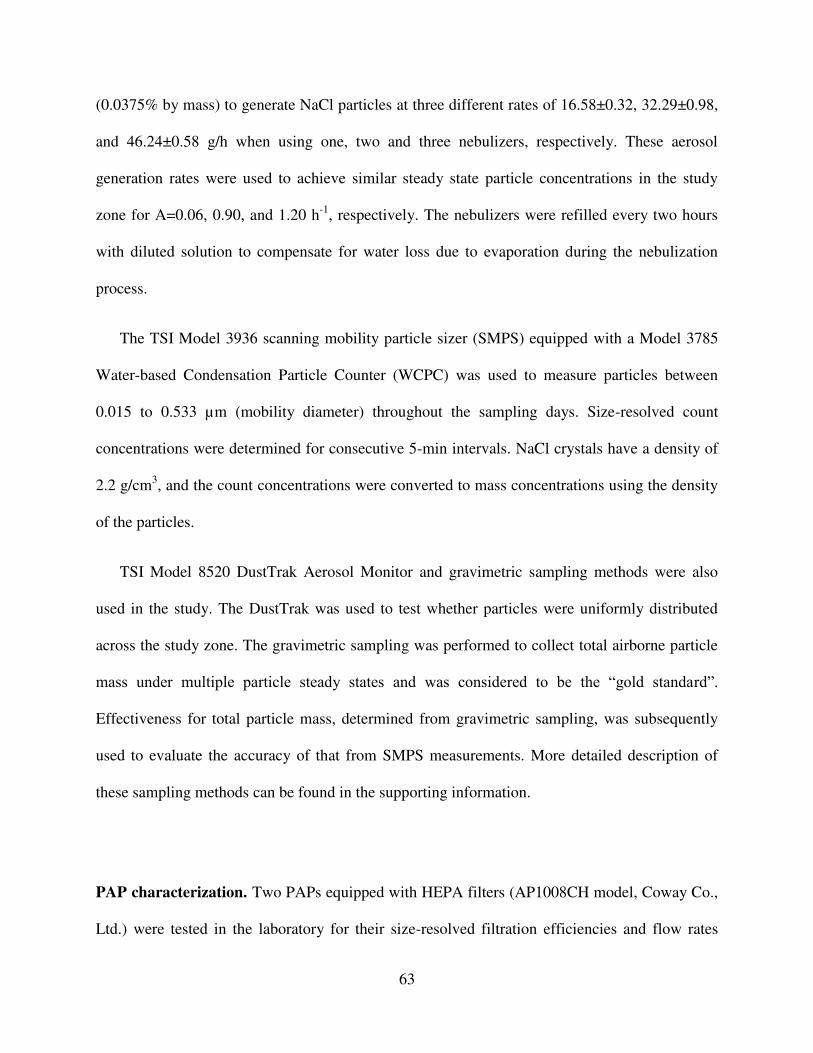
63
(0.0375% by mass) to generate NaCl particles at three different rates of 16.58±0.32, 32.29±0.98,
and 46.24±0.58 g/h when using one, two and three nebulizers, respectively. These aerosol
generation rates were used to achieve similar steady state particle concentrations in the study
zone for A=0.06, 0.90, and 1.20 h-1, respectively. The nebulizers were refilled every two hours
with diluted solution to compensate for water loss due to evaporation during the nebulization
process.
The TSI Model 3936 scanning mobility particle sizer (SMPS) equipped with a Model 3785
Water-based Condensation Particle Counter (WCPC) was used to measure particles between
0.015 to 0.533 µm (mobility diameter) throughout the sampling days. Size-resolved count
concentrations were determined for consecutive 5-min intervals. NaCl crystals have a density of
2.2 g/cm3, and the count concentrations were converted to mass concentrations using the density
of the particles.
TSI Model 8520 DustTrak Aerosol Monitor and gravimetric sampling methods were also
used in the study. The DustTrak was used to test whether particles were uniformly distributed
across the study zone. The gravimetric sampling was performed to collect total airborne particle
mass under multiple particle steady states and was considered to be the “gold standard”.
Effectiveness for total particle mass, determined from gravimetric sampling, was subsequently
used to evaluate the accuracy of that from SMPS measurements. More detailed description of
these sampling methods can be found in the supporting information.
PAP characterization. Two PAPs equipped with HEPA filters (AP1008CH model, Coway Co.,
Ltd.) were tested in the laboratory for their size-resolved filtration efficiencies and flow rates
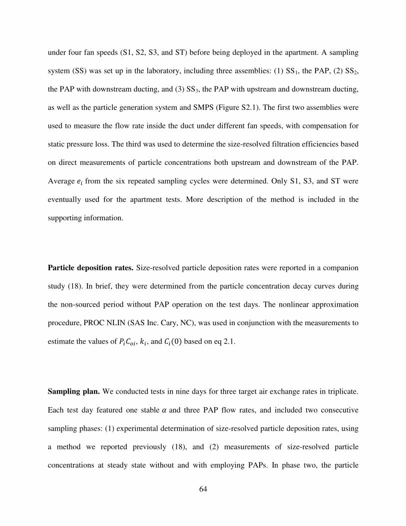
64
under four fan speeds (S1, S2, S3, and ST) before being deployed in the apartment. A sampling
system (SS) was set up in the laboratory, including three assemblies: (1) SS1, the PAP, (2) SS2,
the PAP with downstream ducting, and (3) SS3, the PAP with upstream and downstream ducting,
as well as the particle generation system and SMPS (Figure S2.1). The first two assemblies were
used to measure the flow rate inside the duct under different fan speeds, with compensation for
static pressure loss. The third was used to determine the size-resolved filtration efficiencies based
on direct measurements of particle concentrations both upstream and downstream of the PAP.
Average 結沈 from the six repeated sampling cycles were determined. Only S1, S3, and ST were
eventually used for the apartment tests. More description of the method is included in the
supporting information.
Particle deposition rates. Size-resolved particle deposition rates were reported in a companion
study (18). In brief, they were determined from the particle concentration decay curves during
the non-sourced period without PAP operation on the test days. The nonlinear approximation
procedure, PROC NLIN (SAS Inc. Cary, NC), was used in conjunction with the measurements to
estimate the values of 鶏沈系墜沈, 倦沈, and 系沈岫ど岻 based on eq 2.1.
Sampling plan. We conducted tests in nine days for three target air exchange rates in triplicate.
Each test day featured one stable 糠 and three PAP flow rates, and included two consecutive
sampling phases: (1) experimental determination of size-resolved particle deposition rates, using
a method we reported previously (18), and (2) measurements of size-resolved particle
concentrations at steady state without and with employing PAPs. In phase two, the particle
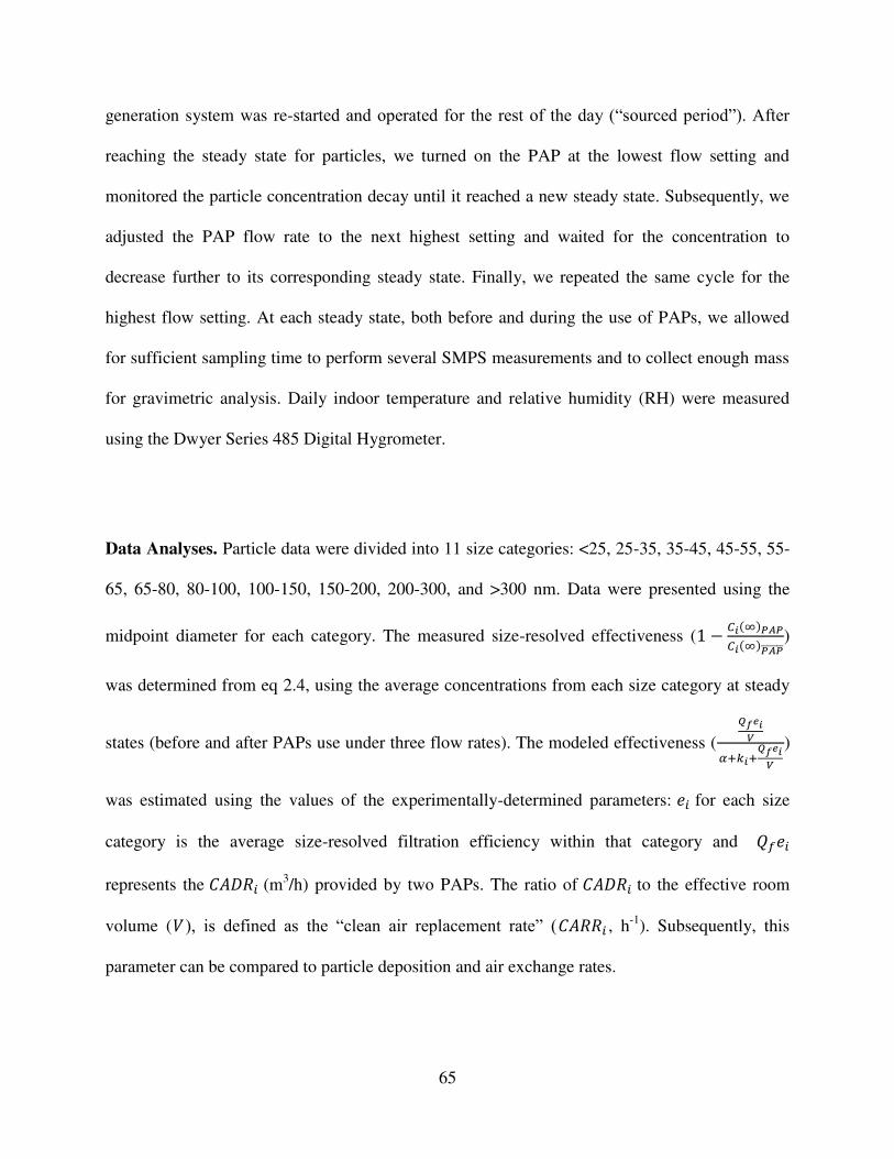
65
generation system was re-started and operated for the rest of the day (“sourced period”). After
reaching the steady state for particles, we turned on the PAP at the lowest flow setting and
monitored the particle concentration decay until it reached a new steady state. Subsequently, we
adjusted the PAP flow rate to the next highest setting and waited for the concentration to
decrease further to its corresponding steady state. Finally, we repeated the same cycle for the
highest flow setting. At each steady state, both before and during the use of PAPs, we allowed
for sufficient sampling time to perform several SMPS measurements and to collect enough mass
for gravimetric analysis. Daily indoor temperature and relative humidity (RH) were measured
using the Dwyer Series 485 Digital Hygrometer.
Data Analyses. Particle data were divided into 11 size categories: <25, 25-35, 35-45, 45-55, 55-
65, 65-80, 80-100, 100-150, 150-200, 200-300, and >300 nm. Data were presented using the
midpoint diameter for each category. The measured size-resolved effectiveness (な 伐 寵日岫著岻鍋豚鍋寵日岫著岻鍋豚鍋博博博博博博博) was determined from eq 2.4, using the average concentrations from each size category at steady
states (before and after PAPs use under three flow rates). The modeled effectiveness (
楢肉賑日楠底袋賃日袋楢肉賑日楠 )
was estimated using the values of the experimentally-determined parameters: 結沈 for each size
category is the average size-resolved filtration efficiency within that category and 芸捗結沈 represents the 系畦経迎沈 (m3/h) provided by two PAPs. The ratio of 系畦経迎沈 to the effective room
volume (撃), is defined as the “clean air replacement rate” (系畦迎迎沈 , h-1). Subsequently, this
parameter can be compared to particle deposition and air exchange rates.
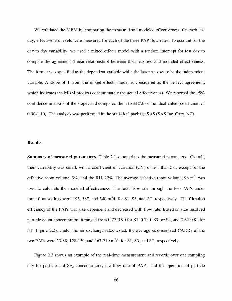
66
We validated the MBM by comparing the measured and modeled effectiveness. On each test
day, effectiveness levels were measured for each of the three PAP flow rates. To account for the
day-to-day variability, we used a mixed effects model with a random intercept for test day to
compare the agreement (linear relationship) between the measured and modeled effectiveness.
The former was specified as the dependent variable while the latter was set to be the independent
variable. A slope of 1 from the mixed effects model is considered as the perfect agreement,
which indicates the MBM predicts consummately the actual effectiveness. We reported the 95%
confidence intervals of the slopes and compared them to ±10% of the ideal value (coefficient of
0.90-1.10). The analysis was performed in the statistical package SAS (SAS Inc. Cary, NC).
Results
Summary of measured parameters. Table 2.1 summarizes the measured parameters. Overall,
their variability was small, with a coefficient of variation (CV) of less than 5%, except for the
effective room volume, 9%, and the RH, 22%. The average effective room volume, 98 m3, was
used to calculate the modeled effectiveness. The total flow rate through the two PAPs under
three flow settings were 195, 387, and 540 m3/h for S1, S3, and ST, respectively. The filtration
efficiency of the PAPs was size-dependent and decreased with flow rate. Based on size-resolved
particle count concentration, it ranged from 0.77-0.90 for S1, 0.73-0.89 for S3, and 0.62-0.81 for
ST (Figure 2.2). Under the air exchange rates tested, the average size-resolved CADRs of the
two PAPs were 75-88, 128-159, and 167-219 m3/h for S1, S3, and ST, respectively.
Figure 2.3 shows an example of the real-time measurement and records over one sampling
day for particle and SF6 concentrations, the flow rate of PAPs, and the operation of particle
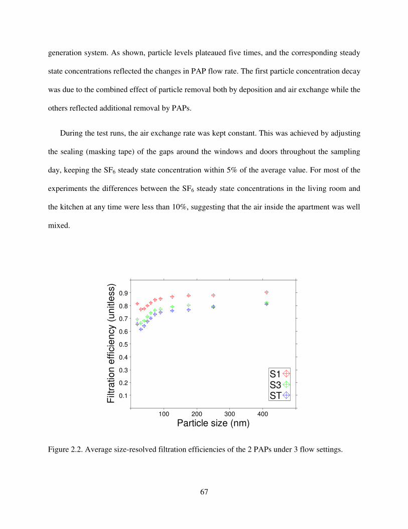
67
generation system. As shown, particle levels plateaued five times, and the corresponding steady
state concentrations reflected the changes in PAP flow rate. The first particle concentration decay
was due to the combined effect of particle removal both by deposition and air exchange while the
others reflected additional removal by PAPs.
During the test runs, the air exchange rate was kept constant. This was achieved by adjusting
the sealing (masking tape) of the gaps around the windows and doors throughout the sampling
day, keeping the SF6 steady state concentration within 5% of the average value. For most of the
experiments the differences between the SF6 steady state concentrations in the living room and
the kitchen at any time were less than 10%, suggesting that the air inside the apartment was well
mixed.
Figure 2.2. Average size-resolved filtration efficiencies of the 2 PAPs under 3 flow settings.
Particle size (nm)
Filt
ratio
n e
ffic
ien
cy (
un
itle
ss)
0.1
0.2
0.3
0.4
0.5
0.6
0.7
0.8
0.9
100 200 300 400
S1S3ST
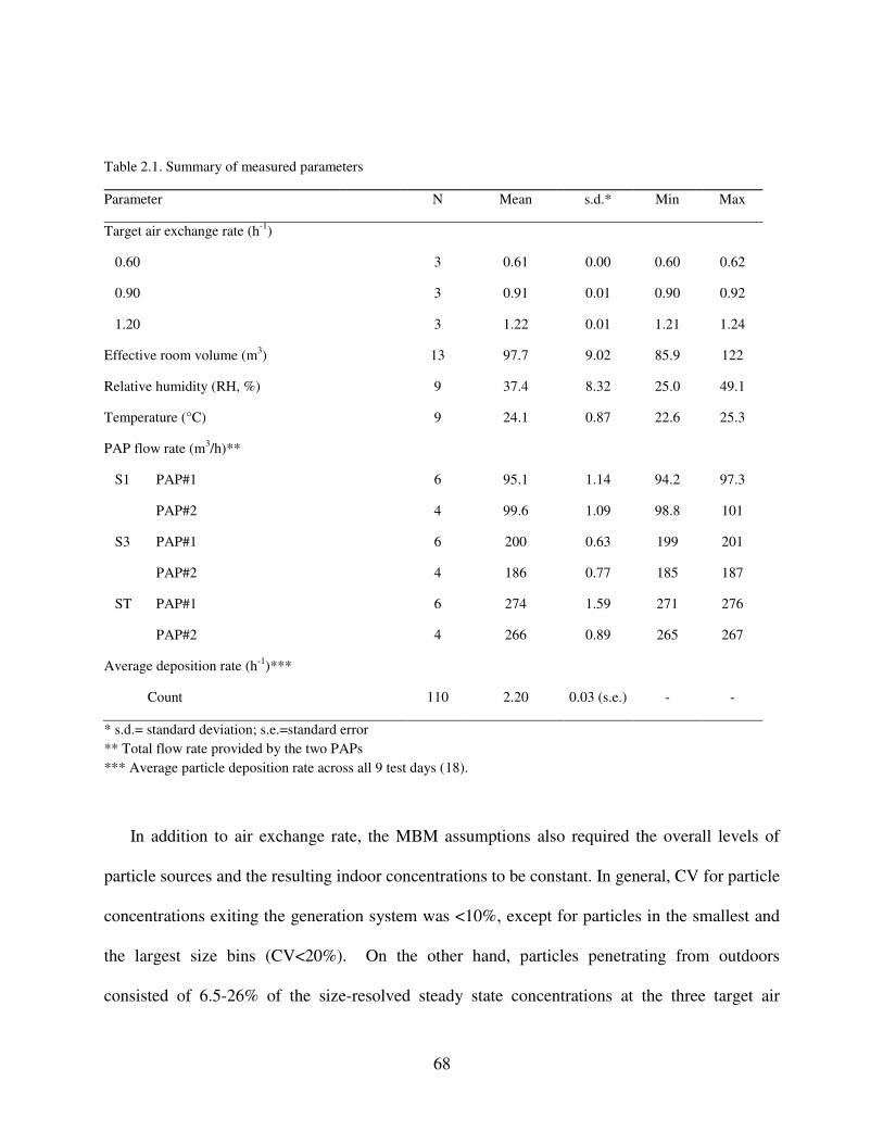
68
Table 2.1. Summary of measured parameters
Parameter N Mean s.d.* Min Max
Target air exchange rate (h-1)
0.60 3 0.61 0.00 0.60 0.62
0.90 3 0.91 0.01 0.90 0.92
1.20 3 1.22 0.01 1.21 1.24
Effective room volume (m3) 13 97.7 9.02 85.9 122
Relative humidity (RH, %) 9 37.4 8.32 25.0 49.1
Temperature (°C) 9 24.1 0.87 22.6 25.3
PAP flow rate (m3/h)**
S1 PAP#1 6 95.1 1.14 94.2 97.3
PAP#2 4 99.6 1.09 98.8 101
S3 PAP#1 6 200 0.63 199 201
PAP#2 4 186 0.77 185 187
ST PAP#1 6 274 1.59 271 276
PAP#2 4 266 0.89 265 267
Average deposition rate (h-1)***
Count 110 2.20 0.03 (s.e.) - -
* s.d.= standard deviation; s.e.=standard error
** Total flow rate provided by the two PAPs
*** Average particle deposition rate across all 9 test days (18).
In addition to air exchange rate, the MBM assumptions also required the overall levels of
particle sources and the resulting indoor concentrations to be constant. In general, CV for particle
concentrations exiting the generation system was <10%, except for particles in the smallest and
the largest size bins (CV<20%). On the other hand, particles penetrating from outdoors
consisted of 6.5-26% of the size-resolved steady state concentrations at the three target air
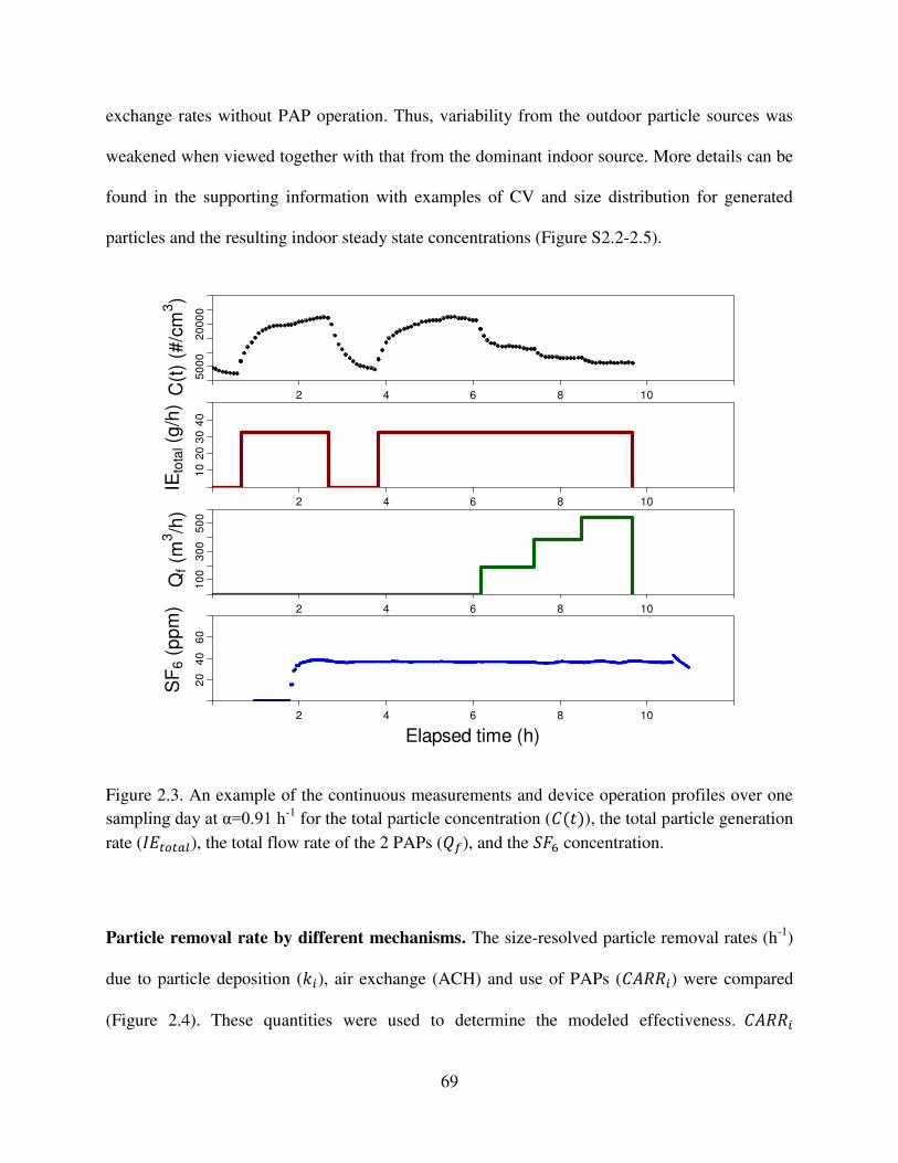
69
exchange rates without PAP operation. Thus, variability from the outdoor particle sources was
weakened when viewed together with that from the dominant indoor source. More details can be
found in the supporting information with examples of CV and size distribution for generated
particles and the resulting indoor steady state concentrations (Figure S2.2-2.5).
Figure 2.3. An example of the continuous measurements and device operation profiles over one
sampling day at g=0.91 h-1 for the total particle concentration (系岫建岻), the total particle generation
rate (荊継痛墜痛銚鎮), the total flow rate of the 2 PAPs (芸捗), and the 鯨繋滞 concentration.
Particle removal rate by different mechanisms. The size-resolved particle removal rates (h-1)
due to particle deposition (倦沈), air exchange (ACH) and use of PAPs (系畦迎迎沈) were compared
(Figure 2.4). These quantities were used to determine the modeled effectiveness. 系畦迎迎沈
Elapsed time (h)
SF
6 (
pp
m)
Qf (m
3/h
)IE
tota
l (g
/h)
C(t
) (#
/cm
3)
20
40
60
2 4 6 8 10
10
03
00
50
0
2 4 6 8 10
10
20
30
40
2 4 6 8 10
50
00
20
00
0
2 4 6 8 10
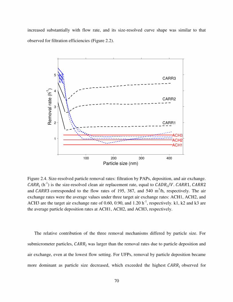
70
increased substantially with flow rate, and its size-resolved curve shape was similar to that
observed for filtration efficiencies (Figure 2.2).
Figure 2.4. Size-resolved particle removal rates: filtration by PAPs, deposition, and air exchange. 系畦迎迎沈 (h-1) is the size-resolved clean air replacement rate, equal to 系畦経迎沈【撃. 系畦迎迎な, 系畦迎迎に
and 系畦迎迎ぬ corresponded to the flow rates of 195, 387, and 540 m3/h, respectively. The air
exchange rates were the average values under three target air exchange rates: ACH1, ACH2, and
ACH3 are the target air exchange rate of 0.60, 0.90, and 1.20 h-1, respectively. k1, k2 and k3 are
the average particle deposition rates at ACH1, ACH2, and ACH3, respectively.
The relative contribution of the three removal mechanisms differed by particle size. For
submicrometer particles, 系畦迎迎沈 was larger than the removal rates due to particle deposition and
air exchange, even at the lowest flow setting. For UFPs, removal by particle deposition became
more dominant as particle size decreased, which exceeded the highest 系畦迎迎沈 observed for
Particle size (nm)
Re
mo
va
l ra
te (
h-1)
1
2
3
4
5
100 200 300 400
ACH1
ACH2
ACH3
CARR1
CARR2
CARR3k1k2k3
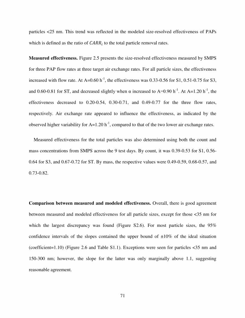
71
particles <25 nm. This trend was reflected in the modeled size-resolved effectiveness of PAPs
which is defined as the ratio of 系畦迎迎沈 to the total particle removal rates.
Measured effectiveness. Figure 2.5 presents the size-resolved effectiveness measured by SMPS
for three PAP flow rates at three target air exchange rates. For all particle sizes, the effectiveness
increased with flow rate. At A=0.60 h-1, the effectiveness was 0.33-0.56 for S1, 0.51-0.75 for S3,
and 0.60-0.81 for ST, and decreased slightly when g increased to A=0.90 h-1. At A=1.20 h-1, the
effectiveness decreased to 0.20-0.54, 0.30-0.71, and 0.49-0.77 for the three flow rates,
respectively. Air exchange rate appeared to influence the effectiveness, as indicated by the
observed higher variability for A=1.20 h-1, compared to that of the two lower air exchange rates.
Measured effectiveness for the total particles was also determined using both the count and
mass concentrations from SMPS across the 9 test days. By count, it was 0.39-0.53 for S1, 0.56-
0.64 for S3, and 0.67-0.72 for ST. By mass, the respective values were 0.49-0.59, 0.68-0.57, and
0.73-0.82.
Comparison between measured and modeled effectiveness. Overall, there is good agreement
between measured and modeled effectiveness for all particle sizes, except for those <35 nm for
which the largest discrepancy was found (Figure S2.6). For most particle sizes, the 95%
confidence intervals of the slopes contained the upper bound of ±10% of the ideal situation
(coefficient=1.10) (Figure 2.6 and Table S1.1). Exceptions were seen for particles <35 nm and
150-300 nm; however, the slope for the latter was only marginally above 1.1, suggesting
reasonable agreement.
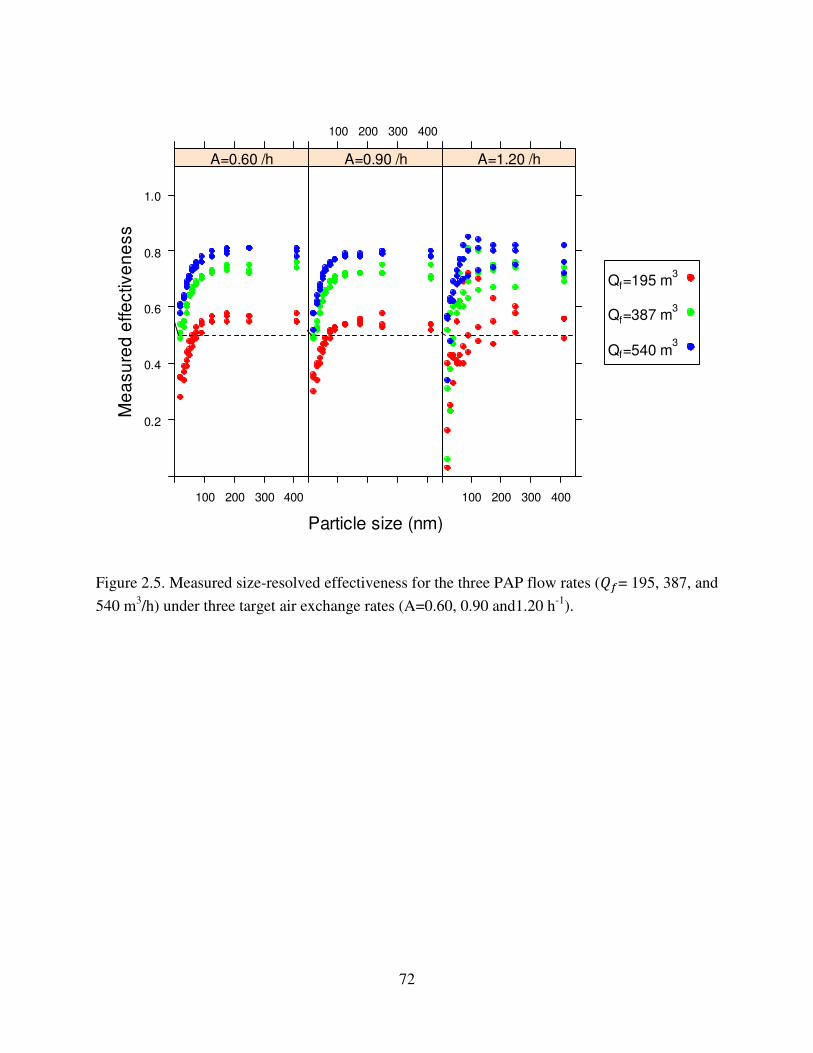
72
Figure 2.5. Measured size-resolved effectiveness for the three PAP flow rates (芸捗= 195, 387, and
540 m3/h) under three target air exchange rates (A=0.60, 0.90 and1.20 h-1).
Particle size (nm)
Me
asu
red
effe
ctiv
en
ess
0.2
0.4
0.6
0.8
1.0
100 200 300 400
A=0.60 /h
100 200 300 400
A=0.90 /h
100 200 300 400
A=1.20 /h
Qf=195 m3
Qf=387 m3
Qf=540 m3
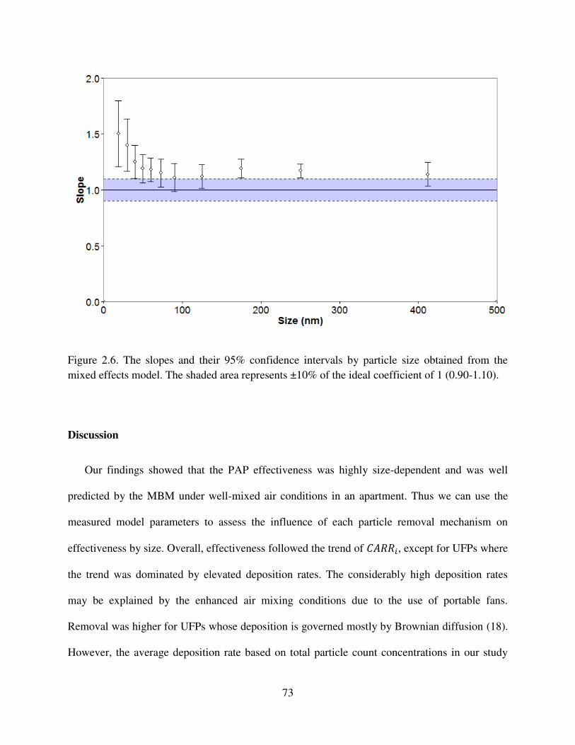
73
Figure 2.6. The slopes and their 95% confidence intervals by particle size obtained from the
mixed effects model. The shaded area represents ±10% of the ideal coefficient of 1 (0.90-1.10).
Discussion
Our findings showed that the PAP effectiveness was highly size-dependent and was well
predicted by the MBM under well-mixed air conditions in an apartment. Thus we can use the
measured model parameters to assess the influence of each particle removal mechanism on
effectiveness by size. Overall, effectiveness followed the trend of 系畦迎迎沈, except for UFPs where
the trend was dominated by elevated deposition rates. The considerably high deposition rates
may be explained by the enhanced air mixing conditions due to the use of portable fans.
Removal was higher for UFPs whose deposition is governed mostly by Brownian diffusion (18).
However, the average deposition rate based on total particle count concentrations in our study
74
(倦=1.17 h-1) was comparable to the average rate of 1.29 for 0.3-1 µm particles estimated in four
homes with smokers (21). Furnishing may also contribute to the elevated deposition rates by
providing additional surface area for deposition (22).
Using the MBM in residential spaces for direct effectiveness measurements is challenging
because of the difficulty to achieve steady state. Most studies measured CADRs in a test
chamber and subsequently used the steady state MBM to estimate the effectiveness for
hypothetical residential indoor spaces (14, 16, 17). Table S2.2 (in the supporting information)
summarizes some of this information, but it is not limited to studies evaluating PAPs with HEPA
filters. In general, studies that modeled effectiveness used the size-resolved deposition rates from
Riley et al. and an air exchange rate ranging from 0.2 to 0.5 h-1, but with varying CADRs and
room volumes (23).
For A=0.60 h-1 the maximum size-resolved effectiveness was observed in submicrometer size
region, and was in general agreement with, but lower than, the maximum effectiveness reported
from other studies (0.60-0.95) (Figure 2.7). The lower effectiveness was mainly due to the
elevated particle deposition rate measured in our study, which was generally at least one order of
magnitude higher than that reported by Riley et al. (23). The overall comparison, on the other
hand, suggested that effectiveness is more comparable across studies for submicrometer particles
where size-resolved effectiveness profile is more flat than that of UFPs.
Because of the size-dependent nature of the effectiveness, the overall effectiveness (all sizes
together) is sensitive to typically wide variations in both particle count and mass size
distributions, which may limit its generalizability and make comparisons more difficult. For
example, using different particle size distributions for dust-mite allergens, Fisk et al. found a
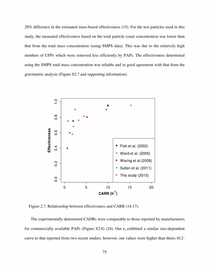
75
20% difference in the estimated mass-based effectiveness (15). For the test particles used in this
study, the measured effectiveness based on the total particle count concentration was lower than
that from the total mass concentration (using SMPS data). This was due to the relatively high
numbers of UFPs which were removed less efficiently by PAPs. The effectiveness determined
using the SMPS total mass concentration was reliable and in good agreement with that from the
gravimetric analysis (Figure S2.7 and supporting information).
Figure 2.7. Relationship between effectiveness and CARR (14-17).
The experimentally determined CADRs were comparable to those reported by manufacturers
for commercially available PAPs (Figure S2.8) (24). Our 結沈 exhibited a similar size-dependent
curve to that reported from two recent studies; however, our values were higher than theirs (0.2-
0 5 10 15 20
0.0
0.2
0.4
0.6
0.8
1.0
CARR (h-1
)
Eff
ec
tiv
en
es
s
Fisk et al. (2002)
Ward et al. (2005)
Waring et al.(2008)
Sultan et al. (2011)
This study (2015)
76
0.8) (14, 16). As expected that HEPA filters have efficiencies >99.97% (25), the observed lower
efficiencies could be explained by air bypassing the filter inside of the PAP and/or the short
circuiting of filtered air (9).
To our knowledge, this is the first study to validate the steady state MBM for predicting the
size-resolved effectiveness of PAPs in a residential setting. Matson validated the MBM using the
non-steady state approach by comparing the difference between calculated and measured mean
values of indoor ultrafine particle concentrations (26). The difference ranged from -16 to 32%
when using deposition rates determined from two residential buildings and two offices in the
model. Nevertheless, no PAP was included in this validation; thus, no direct comparison between
the measured and modeled effectiveness could be inferred from the study. In the current study,
we regressed the measured effectiveness on the modeled one using a mixed effects model. The
slopes from the regression (n=27) by particle size ranged from 1.11±0.06 (80-100 nm) to
1.50±0.14 (<25 nm), providing a quantitative and intuitive way in validating the steady state
MBM.
One of the limitations of our study was the enhanced air mixing condition. The mechanical
mixing enabled achieving a well-mixed condition, but at the same time it might have enhanced
particle deposition, resulting in lower effectiveness compared to other studies. Conversely, the
enhanced air mixing may have increased effectiveness by minimizing short circuiting of filtered
air, compared to conditions without using portable fans. The net effect of these opposite
influences in effectiveness is unknown.
Another limitation was that the findings were based on short-term performance of the PAPs.
One study reported a 25% decrease in CADR after approximately a month of use in a residential
77
bedroom due to the reduction of the PAP air flow rate (13). Another study showed a drop of 7-
14% in air flow after 2 months of continuous operation in smokers’ homes, which was equal to
blocking 33% of the filter area based on simulated tests. The drop was a result of the heavily
loaded pre-filter with fibrous gray dust (21). Nevertheless, decrease in flow rate can be
minimized by routine maintenance such as cleaning the pre-filters regularly and changing the
loaded HEPA filters.
Last but not least, care should be taken when selecting the values of particle deposition rates
for predicting effectiveness because studies have demonstrated possible influences of g on
deposition rates, either on their levels or size-resolved profiles (27-29). The deposition rate we
used in prediction scenarios was the average value determined under a range of 糠 (0.61-1.24 h-1)
which was more or less representative of the overall rates.
In this study, we validated the steady state MBM based on the reasonably good agreement
between the measured and modeled size-resolved effectiveness. We found that effectiveness was
highly size-dependent, and PAP was the dominant removal mechanism for submicrometer
particles, whereas deposition could play a more important role in UFPs removal. The study
design can be applied to investigate the performances of other PAPs as well as the influences of
various parameters on their effectiveness in different residential settings.
78
Bibliography
(1) Peters, A.; Dockery, D.; Muller, J.; Mittleman, M. Increased particulate air pollution and the
triggering of myocardial infarction. Circulation 2001, 103 (23), 2810-2815.
(2) Pope, C.; Thun, M.; Namboodiri, M.; Dockery, D.; Evans, J.; Speizer, F.; Heath, C.
Particulate Air-Pollution as a Predictor of Mortality in a Prospective-Study of Us Adults.
American Journal of Respiratory and Critical Care Medicine 1995, 151 (3), 669-674.
(3) Schwartz, J.; Dockery, D.; Neas, L. Is daily mortality associated specifically with fine
particles? J. Air Waste Manage. Assoc. 1996, 46 (10), 927-939.
(4) Klepeis, N.; Nelson, W.; Ott, W.; Robinson, J.; Tsang, A.; Switzer, P.; Behar, J.; Hern, S.;
Engelmann, W. The National Human Activity Pattern Survey (NHAPS): a resource for assessing
exposure to environmental pollutants. J. Expo. Anal. Environ. Epidemiol. 2001, 11 (3), 231-252;
10.1038/sj.jea.7500165.
(5) Abt, E.; Suh, H.H.; Catalano, P.; Koutrakis, P. Relative contribution of outdoor and indoor
particle sources to indoor concentrations. Environ. Sci. Technol. 2000, 34 (17), 3579-3587;
10.1021/es990348y.
(6) Wallace, L.; Emmerich, S.; Howard-Reed, C. Source strengths of ultrafine and fine particles
due to cooking with a gas stove. Environ. Sci. Technol. 2004, 38 (8), 2304-2311;
10.1021/es0306260.
79
(7) Wallace, L. and Howard-Reed, C. Continuous monitoring of ultrafine, fine, and coarse
particles in a residence for 18 months in 1999-2000. J. Air Waste Manage. Assoc. 2002, 52 (7),
828-844.
(8) Barn, P.; Larson, T.; Noullett, M.; Kennedy, S.; Copes, R.; Brauer, M. Infiltration of forest
fire and residential wood smoke: an evaluation of air cleaner effectiveness. Journal of Exposure
Science and Environmental Epidemiology 2008, 18 (5), 503-511; 10.1038/sj.jes.7500640.
(9) Shaughnessy, R. and Sextro, R. What is an effective portable air cleaning device? A review.
Journal of Occupational and Environmental Hygiene 2006, 3 (4), 169-181;
10.1080/15459620600580129.
(10) Sublett, J.L. Effectiveness of Air Filters and Air Cleaners in Allergic Respiratory Diseases:
A Review of the Recent Literature. Current Allergy and Asthma Reports 2011, 11 (5), 395-402;
10.1007/s11882-011-0208-5.
(11) Association of Home Appliance Manufacturers (AHAM) <br />Standard ANSI/AHAM AC-
1-2006, method for measuring performance of portable household electric room<br />air
cleaners. Association of Home Appliance Manufacturers: Washington, DC, 2006; .
(12) Offermann, F.; Sextro, R.; Fisk, W.; Grimsrud, D.; Nazaroff, W.; Nero, A.; Revzan, K.;
Yater, J. Control of Respirable Particles in Indoor Air with Portable Air Cleaners. Atmos.
Environ. 1985, 19 (11), 1761-1771; 10.1016/0004-6981(85)90003-4.
80
(13) Shaughnessy, R.; Levetin, E.; Blocker, J.; Sublette, K. Effectiveness of Portable Indoor Air
Cleaners - Sensory Testing Results. Indoor Air-International Journal of Indoor Air Quality and
Climate 1994, 4 (3), 179-188; 10.1111/j.1600-0668.1994.t01-1-00006.x.
(14) Sultan, Z.M.; Nilsson, G.J.; Magee, R.J. Removal of ultrafine particles in indoor air:
Performance of various portable air cleaner technologies. Hvac&R Research 2011, 17 (4), 513-
525; 10.1080/10789669.2011.579219.
(15) Fisk, W.; Faulkner, D.; Palonen, J.; Seppanen, O. Performance and costs of particle air
filtration technologies. Indoor Air 2002, 12 (4), 223-234; 10.1034/j.1600-0668.2002.01136.x.
(16) Waring, M.S.; Siegel, J.A.; Corsi, R.L. Ultrafine particle removal and generation by
portable air cleaners. Atmos. Environ. 2008, 42 (20), 5003-5014;
10.1016/j.atmosenv.2008.02.011.
(17) Ward, M.; Siegel, J.; Corsi, R. The effectiveness of stand alone air cleaners for shelter-in-
place. Indoor Air 2005, 15 (2), 127-134; 10.1111/j.1600-0668.2004.00326.x.
(18) Lee, W.; Wolfson, J.M.; Catalano, P.J.; Rudnick, S.N.; Koutrakis, P. Size-Resolved
Deposition Rates for Ultrafine and Submicrometer Particles in a Residential Housing Unit.
Environ. Sci. Technol. 2014, 48 (17), 10282-10290; 10.1021/es502278k.
(19) Nazaroff, W.W. Effectiveness of air cleaning technologies, In Anonymous ; SIY Indoor Air
Information Oy: Helsinki, Finland., 2000; Vol.2 pp. 49-72.
81
(20) ASTM Standard Test Method for Determining Air Change in a Single Zone by Means of a
Tracer Gas Dilution. E741-00. American Society for Testing and Materials International: West
Conshohocken, Pennsylvania, 2001; .
(21) Batterman, S.; Godwin, C.; Jia, C. Long duration tests of room air filters in cigarette
smokers' homes. Environ. Sci. Technol. 2005, 39 (18), 7260-7268; 10.1021/es048951q.
(22) Thatcher, T.L.; Lai, A.C.K.; Moreno-Jackson, R.; Sextro, R.G.; Nazaroff, W.W. Effects of
room furnishings and air speed on particle deposition rates indoors. Atmos. Environ. 2002, 36
(11), 1811-1819; 10.1016/S1352-2310(02)00157-7.
(23) Riley, W.; McKone, T.; Lai, A.; Nazaroff, W. Indoor particulate matter of outdoor origin:
Importance of size-dependent removal mechanisms. Environ. Sci. Technol. 2002, 36 (2), 200-
207; 10.1021/es010723y.
(24) Anonymous Association of Home Appliance Manufacturers (AHAM) Verification Program.
(25) Department of Energy (DOE) Specification for HEPA Filters Used by DOE Contractors.
DOE-STD-3020-97 <br /> . U.S. Department of Energy: Washington, DC, 1997; .
(26) Matson, U. Comparison of the modelling and the experimental results on concentrations of
ultra-fine particles indoors. Build. Environ. 2005, 40 (7), 996-1002;
10.1016/j.buildenv.2004.09.001.
(27) Allen, R.; Larson, T.; Sheppard, L.; Wallace, L.; Liu, L. Use of real-time light scattering
data to estimate the contribution of infiltrated and indoor-generated particles to indoor air.
Environ. Sci. Technol. 2003, 37 (16), 3484-3492; 10.1021/es021007e.
82
(28) He, C.R.; Morawska, L.; Gilbert, D. Particle deposition rates in residential houses. Atmos.
Environ. 2005, 39 (21), 3891-3899; 10.1016/j.atmosenv.2005.03.016.
(29) Rim, D.; Wallace, L.A.; Persily, A.K. Indoor Ultrafine Particles of Outdoor Origin:
Importance of Window Opening Area and Fan Operation Condition. Environ. Sci. Technol.
2013, 47 (4), 1922-1929; 10.1021/es303613e.
83
Supporting information (SI)
Placement of the devices. The apartment layout is fairly symmetric with the bathroom in the
middle, one bedroom and the living room on one side, and the second bedroom and the kitchen
on the other side (Figure 2.1). Both the particle and SF6 generation systems were placed in the
middle of the hallway against the wall. A table fan was used to disperse the SF6 from the source
into the hallway. One box fan was set up at one end of the hallway to blow the air towards the
living room while a second one was set to blow the air towards the kitchen. This arrangement
was to facilitate the distribution of the particles and SF6 to both sides of the room from the
sources.
In the living room, another box fan was placed in the diagonal from the hallway and blew
towards the neighboring corner for air mixing. We located one SF6 monitor and the gravimetric
sampling assembly in the center of the living room, while the Scanning Mobility Particle Sizer
(SMPS) was located slightly further towards the wall. The air purifier was placed at a moderate
distance away from the box fan in the hallway and a shorter distance from the SF6 monitor. A
table fan was employed to blow at the outlet of the air purifier to move filtered air to the room
and minimize re-circulation of the filtered air back into the inlet without being distributed in the
room. The placement of instruments and the fans were identical in the kitchen as it was for the
living room, except for the devices for particle measurements. Under this arrangement, the
particle concentration was determined to be uniform in the study zone based on DustTrak
measurements in additional tests.
84
Adjustment to achieve constant air exchange rate. There was no air conditioning system in
the apartment, and heating was provided by hydronic radiant heating system. Ventilation was
normally through the opening or cracks of windows, doors, and the two small vents that
exhausted indoor air to outdoors. During the sampling period, these openings were tightly closed
and sealed using masking tape. To minimize potential bias in indoor measurements due to the
interference of air inside the space excluded from the study zone, namely the bedrooms and the
bathroom, the windows of the bedrooms were fully open to ensure the particle concentration was
as close as that from outdoors. In principle, adjustment on the taping was made on the door that
led to immediate outdoor environment, which was the patio door in the living room; whereas on
the kitchen side, the bedroom door was a better choice because of limited ventilation in the lobby
outside the entrance door. By removing the masking tape or re-sealing the gaps, we continuously
adjusted the steady state SF6 concentration to the constant level that corresponded to the desired
air exchange rate. More details of the method can be found elsewhere (18).
Measurements of particles. The DustTrak was originally considered as one of the primary
devices for particle measurements in our study due to its portability. However, we found the
calibration ratio between the DustTrak and SMPS measurements varied by day and the various
levels of steady state concentrations of the particles on site, suggesting that the DustTrak
measurement was highly sensitive to the change in particle size distribution. As a result, it was
used only to check if the particles were uniformly distributed across the study zone by measuring
particle concentrations at steady state in multiple locations in the apartment.
85
The gravimetric sampling method provides the average particle mass concentrations over the
sampling time. It was used to collect total suspended particles over the multiple particle steady
states to verify the mass-based effectiveness determined from SMPS measurements (as
integrated samples). A 37 mm 2 たm PTFE filter was placed inside the Harvard Impactor (Air
Diagnostics and Engineering, Inc., Harrison, ME) without the impaction plate, where the room
air was drawn through the filter by a vacuum pump at a post-filter flow rate of 25 L/min. Two
identical gravimetric samplers were placed side by side for all measurements. The particle
weight was determined by the pre- and post-weighing of filters using an electronic microbalance
with laboratory blanks. The filter concentration was calculated from the net mass and the
sampling air volume (which equals to flow rate multiplied by sampling time). The concentrations
acquired from the two parallel samplers were averaged to get a representative mass concentration
of the corresponding steady state.
Characterization of the portable air purifier (PAP). The air purifier had one slit (33 cm x3
cm) on each side that allowed air to be drawn in, pass through a series of particle filters (pre-
filters and the HEPA filter), and return to the room from the exit on the rear side of the device. A
removable front cover was used to access the particle filters for routine replacement. To avoid
damaging the cover for the purpose of laboratory tests, we made a replacement cover with the
same size and a hole in the middle for upstream duct connection. A sampling system (SS) which
included three subsets was set up in the laboratory for the measurements (Figure S2.1). The flow
rates were determined by first recording the pressure drop across the filter of the free-standing air
purifier (SS1), followed by measuring the centerline air velocity inside the duct of SS2 using an
air velocity meter (Velocicalc Model 8345, TSI. Inc., Shoreview, MN). A blower with adjustable
86
fan speed was installed in-line at the end of the duct to overcome the resistance and compensate
for the additional pressure loss due to the addition of the duct, using pressure drop measurements
from SS1 as reference. The measurements were made from the lowest (S1) to the highest (ST)
fan speed of the air purifier for five cycles for the pressure drop and six cycles for the centerline
air velocity in the duct where the average values were used in conjunction with the cross-
sectional area of the duct to determine the four flow rates for each air purifier. The resulting flow
rates were considered as the actual flow rates for the PAP and were set as the target flow rates
when we determined the size-resolved filtration efficiencies with SS3.
Filtration efficiency (結沈) is a measure of the proportion of particles removed by the PAP and
is dependent on particle size (eq S2.1). It was known to have an inverse relationship with air
speed (flow rate), and thus should be determined separately under each fan speed (30).
結沈 噺 な 伐 寵日┸日韮如賑禰寵日┸任祢禰如賑禰 (S2.1)
Where :
系沈┸沈津鎮勅痛 is the particle concentration in the pre-filtered air for particles in the 件痛朕 size category
系沈┸墜通痛鎮勅痛 is the particle concentration in the filtered air for particles in the 件痛朕 size category
87
To measure 系沈┸沈津鎮勅痛 and 系沈┸墜通痛鎮勅痛, we added an additional duct to the upstream of the PAP and
adjusted the downstream end-of-the-duct fan to compensate for the flow rates to the target
values. Ultrafine and submicrometer particles were generated using the same nebulization system
as the one in the apartment. The particles were dried with clean, dry air in the mixing chamber
before entering the upstream duct. Each of the upstream and downstream ducts was equipped
with an isokinetic sampling port, inside which the air velocity was nearly the same as that in the
duct, to allow measurements of particle concentrations using the SMPS. The use of isokinetic
probes assures that the size distribution of the measured particles was not distorted in the
measurement process. Each sampling cycle consisted of alternate measurement of particle
concentrations inside the ducts by switching between upstream and downstream sampling ports.
Averages of the size-resolved efficiencies from the six repeated sampling cycles were
determined for each of the four air purifier fan speeds, respectively.
Constant particle generation rate and steady state concentration. Figure S2.2 shows the
coefficient of variation (CV, %) for the size-resolved particle concentrations exiting the three
different combinations of nebulizers, which were measured in the laboratory. The CV was
generally low, except for the smallest and the largest size bins. This was because these two size
bins had lower concentrations (at the tails of the size distribution). Overall, CV <10% suggested
stable and constant generation of particles.
Figure S2.3 shows the CV of the steady state concentrations in the apartment without PAP
operation and at the PAP fan speed of S1, S3, and ST in the nine test days. The variability profile
was similar to that in Figure S2.2. Additionally, both the use of PAPs and higher air exchange
rate could possibly contribute to the variability of concentrations in the largest particle size bin
88
(particles >300 nm). Filtration efficiency was higher for large particles. The highest three values
of CV for particles >300 nm were under the target air exchange of 1.20/h with the use of air
purifiers on the highest two speeds.
Figure S2.4 shows the particle size distribution using the same data as those from Figure
S2.2. Good agreement was observed from the repeated measurements of particle concentrations
and their distribution on the same test day.
Figure S2.5 displays the particle size distribution at steady state under four PAP flow settings
(Qf= 0, 195, 387, and 540 m3/h) in the apartment. We used measurements from one test day as an
example to show the evolution of the size distribution with and without the use of PAPs. The
distribution exhibited similar trend but slightly different among the test days, partially because
we used different combinations of nebulizers for different target air exchange rates (as shown in
Figure S2.4) and of the change in relative humidity on site.
Validation of the SMPS mass data. We calibrated the effectiveness for total particle mass
concentrations from the SMPS measurements using that from the gravimetric method. Figure
S2.7-(a) shows the calibration using all measurements. However, measurements from
gravimetric sampling for one particular day were overall problematic with unreasonably low
mass concentrations. We removed those three measurements and found that the r-squared value
increased from 0.79 to 0.89, but the coefficient (slope) between the two methods remained stable
at around 0.95-0.96 (Figure S2.7-(a) and (b)). We concluded that measurements from SMPS
were reliable.
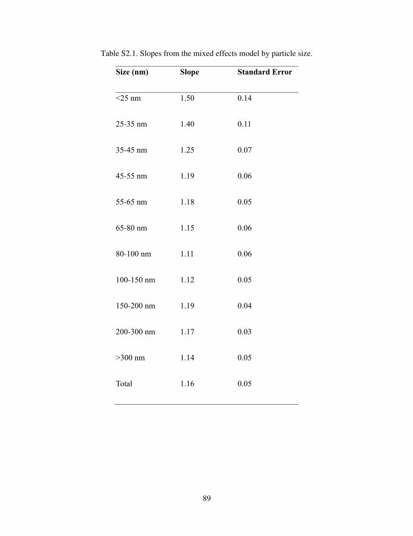
89
Table S2.1. Slopes from the mixed effects model by particle size.
Size (nm) Slope Standard Error
<25 nm 1.50 0.14
25-35 nm 1.40 0.11
35-45 nm 1.25 0.07
45-55 nm 1.19 0.06
55-65 nm 1.18 0.05
65-80 nm 1.15 0.06
80-100 nm 1.11 0.06
100-150 nm 1.12 0.05
150-200 nm 1.19 0.04
200-300 nm 1.17 0.03
>300 nm 1.14 0.05
Total 1.16 0.05
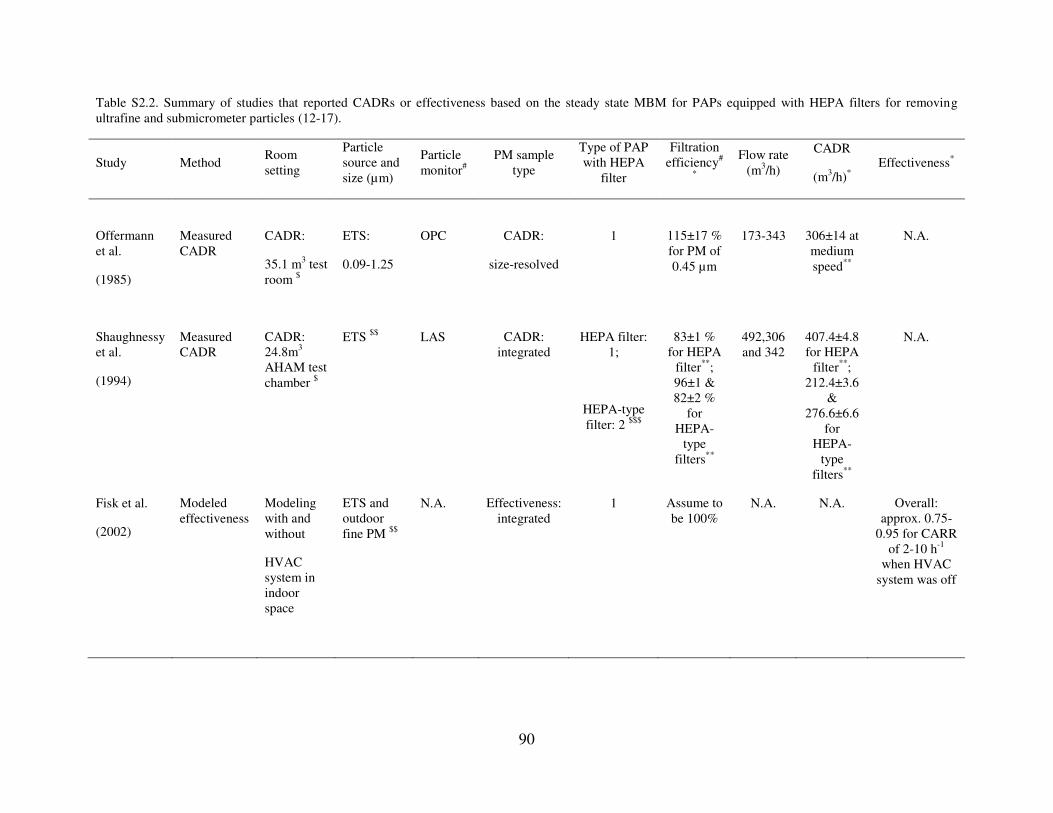
90
Table S2.2. Summary of studies that reported CADRs or effectiveness based on the steady state MBM for PAPs equipped with HEPA filters for removing ultrafine and submicrometer particles (12-17).
Study Method Room setting
Particle source and size (µm)
Particle monitor#
PM sample type
Type of PAP with HEPA
filter
Filtration efficiency#
*
Flow rate (m3/h)
CADR
(m3/h)* Effectiveness*
Offermann et al.
(1985)
Measured CADR
CADR:
35.1 m3 test room $
ETS:
0.09-1.25
OPC
CADR:
size-resolved
1
115±17 % for PM of 0.45 µm
173-343
306±14 at medium speed**
N.A.
Shaughnessy et al.
(1994)
Measured CADR
CADR: 24.8m3 AHAM test chamber $
ETS $$ LAS CADR: integrated
HEPA filter: 1;
HEPA-type filter: 2 $$$
83±1 % for HEPA
filter**; 96±1 & 82±2 %
for HEPA-
type filters**
492,306 and 342
407.4±4.8 for HEPA
filter**; 212.4±3.6
& 276.6±6.6
for HEPA-
type filters**
N.A.
Fisk et al.
(2002)
Modeled effectiveness
Modeling with and without
HVAC system in indoor space
ETS and outdoor fine PM $$
N.A. Effectiveness: integrated
1 Assume to be 100%
N.A. N.A. Overall: approx. 0.75-
0.95 for CARR of 2-10 h-1
when HVAC system was off
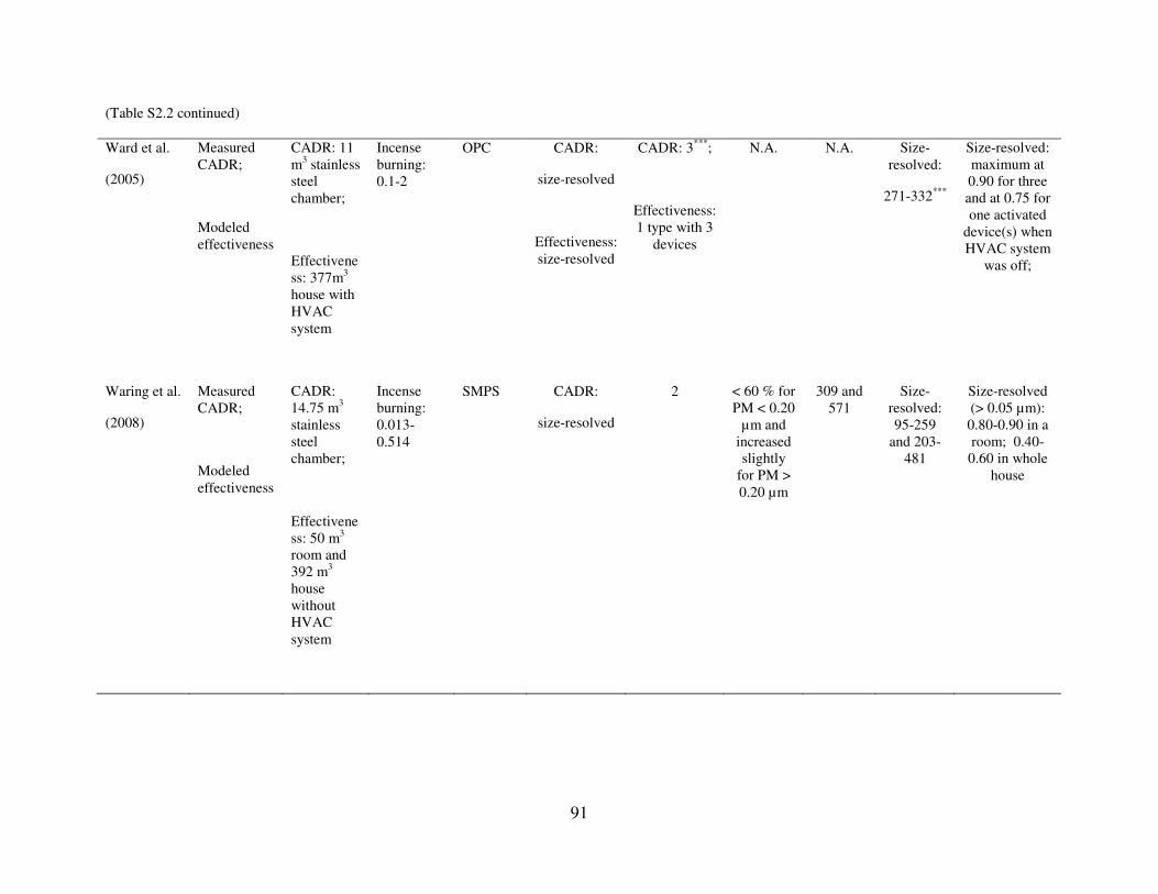
91
(Table S2.2 continued)
Ward et al.
(2005)
Measured CADR;
Modeled effectiveness
CADR: 11 m3 stainless steel chamber;
Effectiveness: 377m3 house with HVAC system
Incense burning: 0.1-2
OPC CADR:
size-resolved
Effectiveness: size-resolved
CADR: 3***;
Effectiveness: 1 type with 3
devices
N.A. N.A. Size-resolved:
271-332***
Size-resolved: maximum at 0.90 for three and at 0.75 for one activated
device(s) when HVAC system
was off;
Waring et al.
(2008)
Measured CADR;
Modeled effectiveness
CADR: 14.75 m3 stainless steel chamber;
Effectiveness: 50 m3 room and 392 m3 house without HVAC system
Incense burning: 0.013-0.514
SMPS CADR:
size-resolved
2 < 60 % for PM < 0.20
µm and increased slightly
for PM > 0.20 µm
309 and 571
Size-resolved: 95-259
and 203-481
Size-resolved (> 0.05 µm): 0.80-0.90 in a room; 0.40-0.60 in whole
house
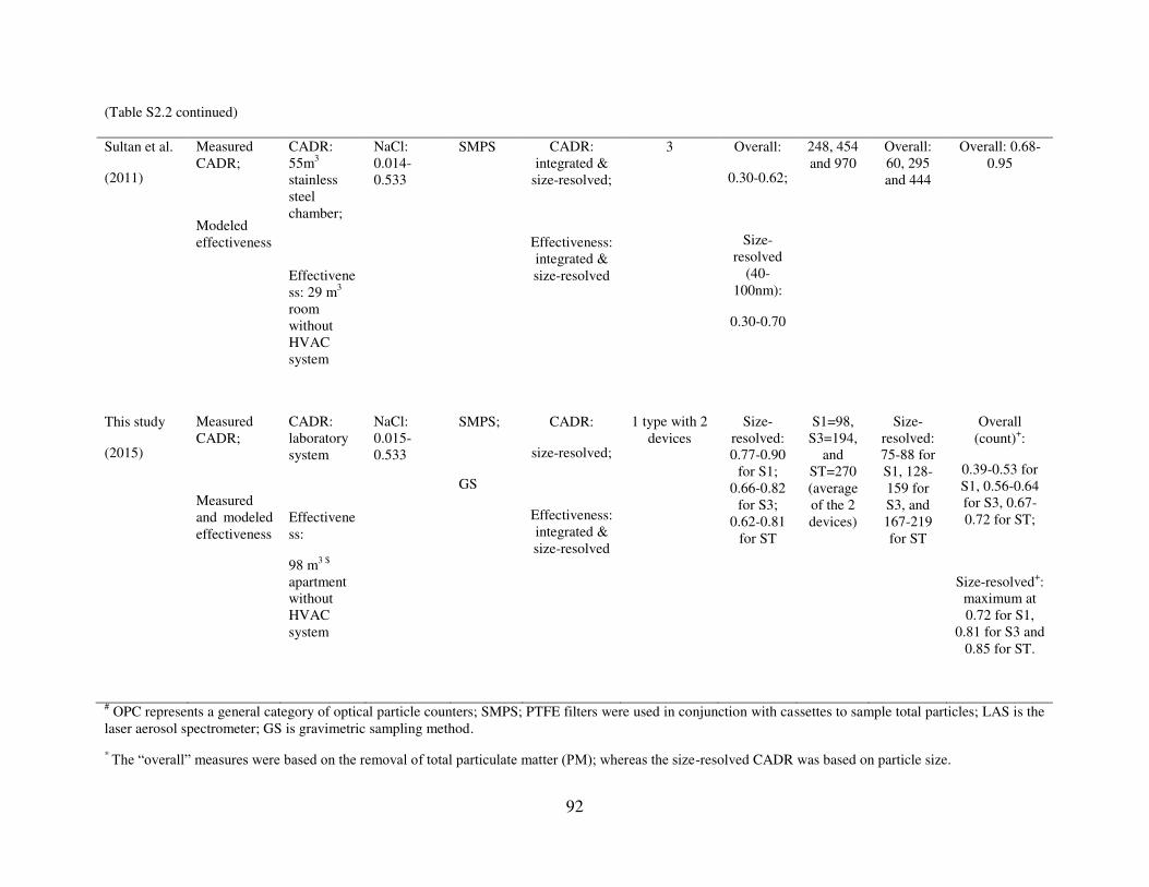
92
(Table S2.2 continued)
Sultan et al.
(2011)
Measured CADR;
Modeled effectiveness
CADR: 55m3 stainless steel chamber;
Effectiveness: 29 m3 room without HVAC system
NaCl: 0.014-0.533
SMPS CADR: integrated &
size-resolved;
Effectiveness: integrated & size-resolved
3 Overall:
0.30-0.62;
Size-resolved
(40-100nm):
0.30-0.70
248, 454 and 970
Overall: 60, 295 and 444
Overall: 0.68-0.95
This study
(2015)
Measured CADR;
Measured and modeled effectiveness
CADR: laboratory system
Effectiveness:
98 m3 $ apartment without HVAC system
NaCl: 0.015-0.533
SMPS;
GS
CADR:
size-resolved;
Effectiveness: integrated & size-resolved
1 type with 2 devices
Size-resolved: 0.77-0.90
for S1; 0.66-0.82
for S3; 0.62-0.81
for ST
S1=98, S3=194,
and ST=270 (average of the 2 devices)
Size-resolved: 75-88 for S1, 128-159 for S3, and 167-219 for ST
Overall (count)+:
0.39-0.53 for S1, 0.56-0.64 for S3, 0.67-0.72 for ST;
Size-resolved+: maximum at 0.72 for S1,
0.81 for S3 and 0.85 for ST.
# OPC represents a general category of optical particle counters; SMPS; PTFE filters were used in conjunction with cassettes to sample total particles; LAS is the laser aerosol spectrometer; GS is gravimetric sampling method.
* The “overall” measures were based on the removal of total particulate matter (PM); whereas the size-resolved CADR was based on particle size.
93
(Table S2.2 continued)
** The range was ± 95% confidence limits from Shaughnessy et al.,13 and ± 90% confidence limits from Offermann et al. (12).
*** The CADR for each particle size was the average value from the three PAPs tested which was used to model the effectiveness (17).
$ It was the effective room volume or the net air space volume. AHAM stands for Association of Home Appliance Manufacturers.
$$ Studies also included other particle sources.
$$$ HEPA-type filters with an efficiency of 95% for particles of 0.3 µm.
+ Determined from SMPS measurements.
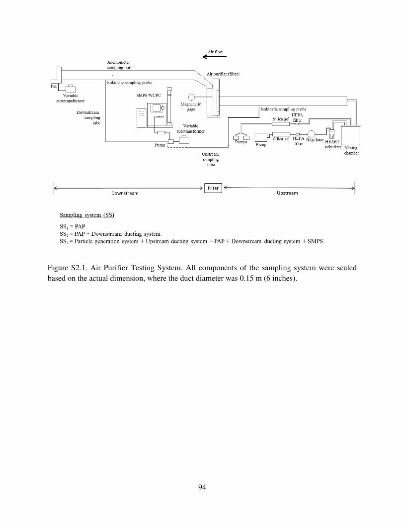
94
Figure S2.1. Air Purifier Testing System. All components of the sampling system were scaled
based on the actual dimension, where the duct diameter was 0.15 m (6 inches).
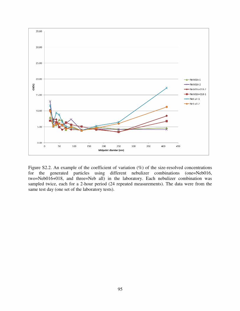
95
Figure S2.2. An example of the coefficient of variation (%) of the size-resolved concentrations for the generated particles using different nebulizer combinations (one=Neb016, two=Neb016+018, and three=Neb all) in the laboratory. Each nebulizer combination was sampled twice, each for a 2-hour period (24 repeated measurements). The data were from the same test day (one set of the laboratory tests).
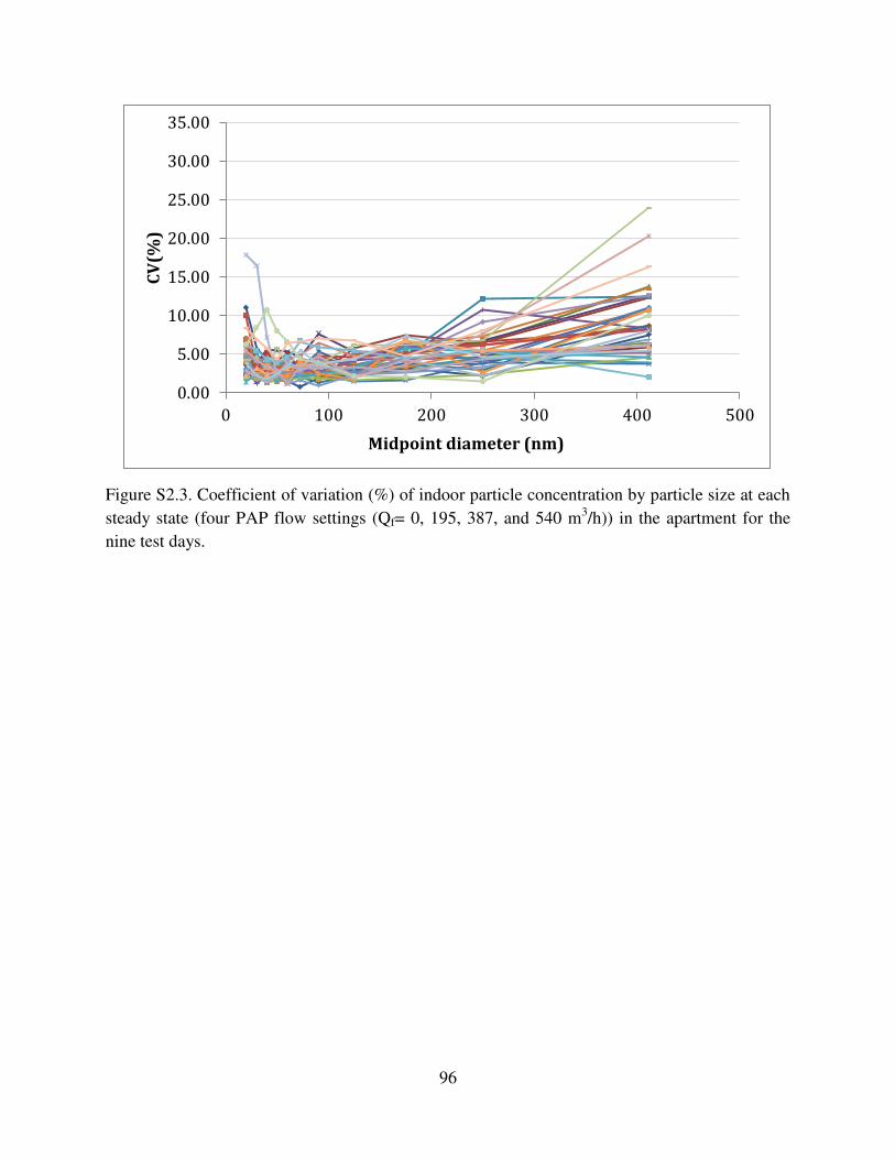
96
Figure S2.3. Coefficient of variation (%) of indoor particle concentration by particle size at each
steady state (four PAP flow settings (Qf= 0, 195, 387, and 540 m3/h)) in the apartment for the
nine test days.
0.00
5.00
10.00
15.00
20.00
25.00
30.00
35.00
0 100 200 300 400 500
CV
(%)
Midpoint diameter (nm)
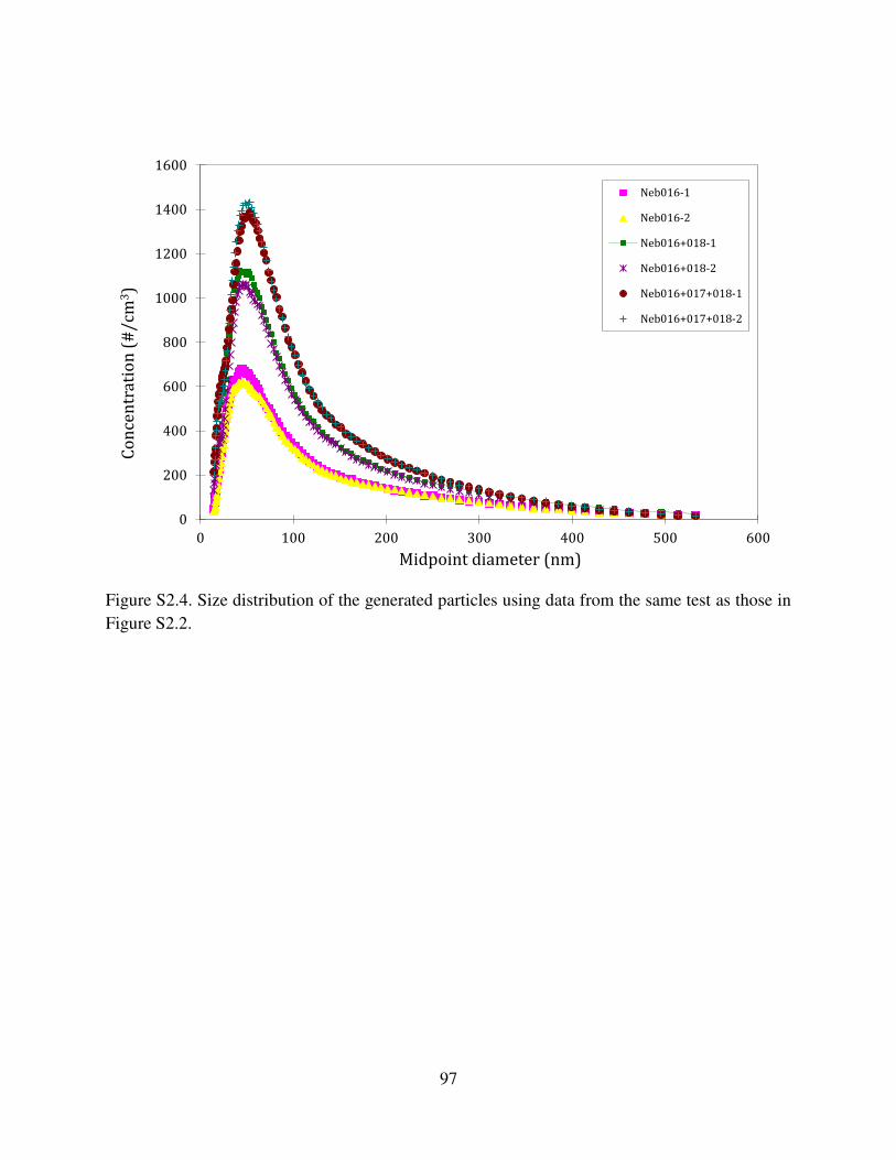
97
Figure S2.4. Size distribution of the generated particles using data from the same test as those in
Figure S2.2.
0
200
400
600
800
1000
1200
1400
1600
0 100 200 300 400 500 600
Co
nce
ntr
ati
on
(#
/cm
3)
Midpoint diameter (nm)
Neb016-1
Neb016-2
Neb016+018-1
Neb016+018-2
Neb016+017+018-1
Neb016+017+018-2
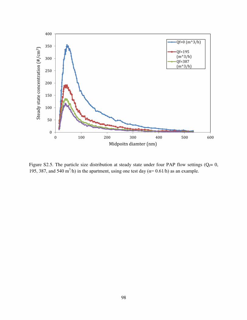
98
Figure S2.5. The particle size distribution at steady state under four PAP flow settings (Qf= 0,
195, 387, and 540 m3/h) in the apartment, using one test day (g= 0.61/h) as an example.
0
50
100
150
200
250
300
350
400
0 100 200 300 400 500 600
Ste
ad
y s
tate
co
nce
ntr
ati
on
(#
/cm
3)
Midpoitn diamter (nm)
Qf=0 (m^3/h)
Qf=195
(m^3/h)
Qf=387
(m^3/h)
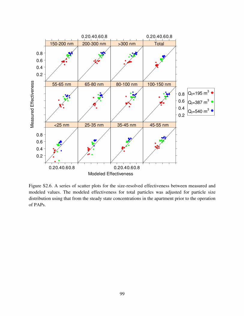
99
Figure S2.6. A series of scatter plots for the size-resolved effectiveness between measured and
modeled values. The modeled effectiveness for total particles was adjusted for particle size
distribution using that from the steady state concentrations in the apartment prior to the operation
of PAPs.
Modeled Effectiveness
Measure
d E
ffectiveness
0.2
0.4
0.6
0.8
0.20.40.60.8
<25 nm 25-35 nm
0.20.40.60.8
35-45 nm 45-55 nm
55-65 nm 65-80 nm 80-100 nm
0.2
0.4
0.6
0.8
100-150 nm
0.2
0.4
0.6
0.8
150-200 nm
0.20.40.60.8
200-300 nm >300 nm
0.20.40.60.8
Total
Qf=195 m3
Qf=387 m3
Qf=540 m3
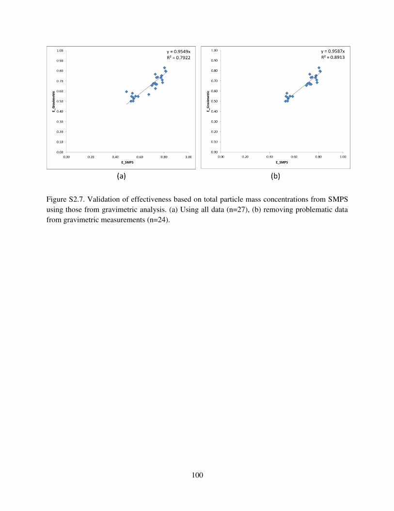
100
Figure S2.7. Validation of effectiveness based on total particle mass concentrations from SMPS
using those from gravimetric analysis. (a) Using all data (n=27), (b) removing problematic data
from gravimetric measurements (n=24).
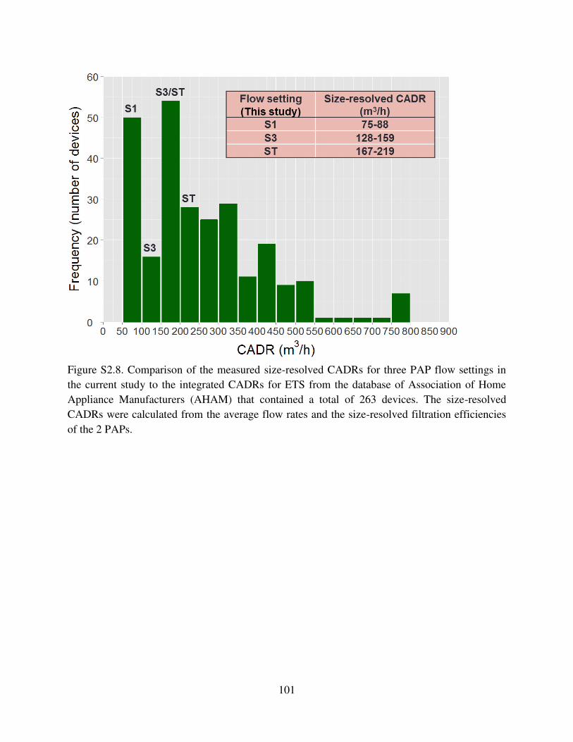
101
Figure S2.8. Comparison of the measured size-resolved CADRs for three PAP flow settings in
the current study to the integrated CADRs for ETS from the database of Association of Home
Appliance Manufacturers (AHAM) that contained a total of 263 devices. The size-resolved
CADRs were calculated from the average flow rates and the size-resolved filtration efficiencies
of the 2 PAPs.

102
CHAPTER 3
Effects of Monthly and Long-term Temperature Change on Indoor Exposure to Outdoor
PM2.5 in the Greater Boston Area
(Working paper)
103
Abstract
In this study we assembled data from two cohorts in the greater Boston area, assessing the
monthly and long-term effect of temperature and other meteorology on Sr, a surrogate of I/O for
PM2.5 in two populations: the whole population with mixed AC usage and the subpopulation of
naturally ventilated homes. We found that Sr was independent of meteorology studied, with the
exception of temperature. Monthly effect of temperature was much more dominant when
compared to long-term effect on Sr, which differed in the two populations. In the future, the
seasonal difference (between summer and winter) in Sr was estimated to be as high as 54% for
naturally ventilated home and 30% for the whole population, using winter as the baseline.
Additionally, future Sr in naturally ventilated homes would be approximately 20% higher
compared to the whole population in summer, whereas the difference was small in winter. We
also observed monthly difference in long-term temperature effect for the naturally ventilated
homes, corresponding to an average of 2.1-2.9 襖 increase in monthly temperature. However,
difference was small with maximum of 7% for Sr in July, using values from the past as the
baseline for comparison. In the future, when given the data on future outdoor PM concentrations,
Sr can be used to independently estimate the outdoor fraction of indoor PM, regardless various
indoor sources. It can subsequently be applied to further assess the modification of Sr on the
relationship between future indoor PM exposure and public health in the greater Boston area.
Key words: Indoor-outdoor sulfur ratio; Temperature; Climate change; Particle Infiltration
104
Introduction
There is a large body of evidence implicating short- and long-term exposures to PM2.5 as a
leading contributor to the global burden of disease (1). Individual exposure to PM2.5 can vary
considerably, and is subject to modification from physical, behavioral, and socio-demographic
factors. Notably, since most individuals spend the majority of their time indoors (2), total
exposure to PM2.5 occurs for many people while indoors (3).
Home ventilation has been identified as a central driver of indoor PM2.5 levels (4, 5).
Specifically, home ventilation drives the composition of indoor PM2.5 levels through its
competing effects on increasing ambient particle infiltration and reducing the source strengths of
indoor particle contributions (6). Ventilation is commonly expressed as the air exchange rate, or
the number of times an indoor air volume is replaced by outdoor air over time (e.g., per hour).
Although limited, previous studies have suggested that air exchange rate may modify air
pollution-related short- and long-term health risk (7-12). In an important initial investigation,
Janssen et al. (11) found that city-specific air conditioning (AC) prevalence estimates in 14 US
locations were inversely associated with city-specific effect estimates of outdoor PM2.5 on
hospital admissions for heart and lung disease. That study assumed that homes with central AC
had lower air exchange rate as compared to homes that opened windows for ventilation.
Recently, Sarnat et al. (13) reported significant, positive interactions between air exchange rate
and several air pollutants, including PM2.5, on asthma emergency department visits in Atlanta.
The observed modification of outdoor PM2.5 health effects by air exchange rate may be due, in
part, to its impact on driving greater exposures to particles from outdoor sources.
105
Ambient temperature has been reported to be one of the driving forces for occupant behavior
in window opening and AC operation (14, 15), which greatly influence air exchange rate. Air
exchange rate is also associated with building envelope tightness and wind speed (16-18). Given
the influence of meteorology on air exchanger rate from physical mechanism through building
envelope or/and residential behavior, projected changes in ambient temperature associated with
monthly (or seasonal) and long-term global climate trends may affect population exposures to
PM2.5, which in turn could affect their related disease burden. No studies to our knowledge have
examined this to date.
The objective of this study was, therefore, to quantify the change of indoor exposure to
outdoor PM as it relates to ambient temperature change resulting from monthly variation and
climate change for the population in the greater Boston area. We hypothesized that variation in
ambient temperatures associated with monthly change, highlighted by summer-winter difference,
and long-term climate change would impact home air exchange rates, leading to either decreased
air exchange rates during the increasingly warmer months with AC usage, or increased air
exchange rates due to open windows, or a combination of both. These changes would, in turn,
alter the contributions of outdoor particle sources to indoor air quality, and subsequently lead to
differential effects of PM2.5 exposures by month or season, and in the future relative to the past.
To test the hypothesis, we assembled a large database to establish relationships between the
indoor-outdoor sulfur ratio, Sr, and ambient temperature for the whole study population, as well
as a subpopulation without AC usage. Sr has been widely accepted as a means of approximating
outdoor PM2.5 infiltration fraction by many studies, which are summarized in a recently
published review article from Diapouli et al. (19, 20). Sulfur is a unique tracer for studying the
origin of indoor PM2.5 particles for the following reasons: 1) in general, it does not have indoor
106
sources; 2) it is a regional pollutant, and thus it exhibits very little spatial variability. This makes
possible the use of outdoor measurements at a centrally located supersite to apply for the entire
region; 3) it is a major constituent of PM2.5 and its infiltration and deposition rates are similar to
those of PM2.5, and; 4) it is a very stable pollutant that can be measured readily and accurately
(21). We then used projected past and future temperature to predict their corresponding Sr over
twenty years, respectively. Results from this study were expected to contribute to an initial
understanding of the role of ambient temperature and the impact of monthly variation in
meteorology and climate change on residential exposure to outdoor PM2.5.
Materials and methods
Mass balance model (MBM). We used the same mass balance equation as that in Chapter 1 and
2 for indoor PM concentration. In the presence of indoor sources, the indoor PM2.5
concentrations at steady state can be determined as
系沈津鳥 噺 繋墜 髪 繋沈津鳥 噺 底牒寵任底袋賃 髪 内曇楠底袋賃 (3.1)
where, Cind and Co are the concentrations of particles indoors and outdoors, respectively (µg/m3);
Fo and Find are the concentrations of indoor particles of indoor and outdoor origin, respectively
(µg/m3); Į is the home air exchange rate (hr-1); P is the particle penetration coefficient
(dimensionless); k is the deposition rate of particles indoors (hr-1); IE is the emission rate of
indoor particle sources (µg/hr); and 撃 is the house volume (m3).
Sulfur is the major constituent of PM2.5, as reported from studies conducted in the greater
Boston area (13). We could therefore replace PM2.5 in eq 3.1 by sulfur concentration. Given the
107
lack of indoor sulfur sources, eq 3.1 can be rearranged to express the indoor-outdoor sulfur ratio
(Sr), also known as the sulfur based infiltration factor:
鯨追 噺 聴日韮匂聴任 噺 底牒底袋賃 (3.2)
where, Sind and So are the indoor and outdoor concentrations of sulfur, respectively (µg/m3). In
this study, Sr was equal to the PM2.5 infiltration factor which was the fraction of outdoor particles
present indoors, and could be linked to indoor exposure to outdoor PM2.5 on the population level.
Study population. We assembled a large database of archived (retrospective) indoor and
outdoor PM2.5 mass and sulfur concentrations collected at homes from two cohorts between 2006
and 2010 in Boston, MA烉the Diabetes, Cardiac Disease, and Pollution Vulnerability (DCDPV)
Study (20, 22) and the Normative Aging Study (NAS) (20, 23). DCDPV was conducted to assess
the relation of traffic related and transported air pollution to vascular/endothelial, inflammatory
and autonomic outcomes, and evaluated differences in effects based on particle composition. 70
homes were selected for a repeated measurements study. Exclusion criteria included factors that
might complicate estimation of pollution exposures (e.g., ambient air pollution measurements,
such as second hand smoking at home, living more than 25 km away from the central Supersite),
as well as certain highly compromising conditions or diseases (22). Integrated air pollutant
samples were collected inside 70 homes for 6 days. For most of these homes 4-5 samples were
collected at least once during each season. A total of 341 samples were collected between 2006 -
2010 and were used in our study.
The NAS was linked to the original NAS which is a longitudinal study of aging in Eastern
Massachusetts established in 1963 by the Veterans Administration (VA) with 2,280 community-
108
dwelling, healthy men enrolled between 1963 and 1968 (20, 23). During 2006-2010, 321
samples were collected from 270 homes for approximately 7 days, where most homes were
sampled once, except for 50 homes sampled twice.
Altogether, we assembled 662 samples from 340 homes collected across all months in the
greater Boston area in this study. Selected variables included home location (longitude and
latitude), air pollutant sampling duration, weather parameters recorded from the central sites
(Harvard Supersite and weather station at Boston Logan Airport), average indoor air pollutant
concentrations over sampling durations, air conditioning (AC) usage (AC=1 for yes and AC=0
for no), and window open status (yes or no). This database was used to establish relationships
between ambient temperature and indoor particle exposure to ambient particles (Sr) using the
exposure models.
Air pollution measurements. Indoor PM2.5 samples were collected using a custom-made
Harvard sampling system in both cohort studies (20, 22, 23). The sampler was sent to the
subject’s home by express shipping in a specially constructed container the week before their
health examination appointment. The subject was instructed to place the sampler in the main
activity room of the house (other than a kitchen), typically the family room or living room. The
sampler started automatically when plugged in, and after one week, the sampler was unplugged.
The subject then brought the sampler to their health exam, or called for an express shipping pick-
up. The sampler collected PM2.5 particles on a Teflon filter which was then analyzed for PM2.5
mass concentration and other particle components, including sulfur concentration.
109
As mentioned preciously, sulfur is a regional pollutant and is relatively stable. We used the
ambient sulfur measurements at the central Supersite at the Harvard University Countway
Library to represent the outdoor sulfur concentrations for each home in the greater Boston area,
corresponding to their sampling durations of indoor air pollutants. Measurements from the
Supersite were not affected by local point sources.
Meteorology data. The original data sets for the two cohorts included meteorological records
from central sites (Harvard Supersite or weather stations at Boston Logan Airport). In the
preliminary analysis, we compared the meteorological measurements from Boston Logan Airport
in the Global Summary of Days (GSOD) database to the Harvard Supersite values and found that
wind speed varied substantially due to geographic differences between the oceanside and more
inland locations of the monitoring sites. Temperature, on the other hand, was relatively
consistent.
To minimize the potential bias in meteorology records due to the varying distance of the
home locations to the central sites, we used meteorology data from the North American Regional
Reanalysis (NARR) database. NARR is conducted by National Centers for Environmental
Prediction (NCEP) and provides reanalysis data from 1979 to near present. It produces historical
high resolution (32 x32 km per grid) data for North America, which is assimilated from
observational sources including surface, rawinsonde, satellite and aircraft (24). In this study, we
matched the centroids of the grids in NARR to the home locations. Meteorology from the grid
with the shortest distance to a home was used to provide representative weather data for that
home for the same sampling period. The selected meteorological parameters included average
110
daily temperature (measured at 2 m above the surface), wind speed (measured at 10 m above the
surface), precipitation and relative humidity (measured at 2 m above the surface). Maximum and
minimum daily temperature was determined from the 3-h averages in the same database.
Negative values for precipitation were replaced by 0.
Climate forecast model. We forecasted temperature, wind speed, relative humidity, and
precipitation in Boston for two 20-year periods: 1981-2000 (the past) and 2046-2065 (the future).
Forecasts for both the past and the future were made using data archived for the Coupled Model
Inter-comparison Project Phase 5 (CMIP5), an initiative of the Intergovernmental Panel on
Climate Change Fifth Assessment Report (25). This database contains projected meteorology
generated by a suite of climate models for a range of socioeconomic scenarios at a 100x100 km
resolution. We selected 15 CMIP5 models because they provided daily averages for the selected
weather parameters. Predictions were performed for a set of scenarios which met specified
targets for anthropogenic radiative forcing, a measure of climate change (26). These scenarios,
known as the Representative Concentration Pathways (RCPs), aim for radiative forcings in the
year 2100 of 8.5 Wm-2 (RCP8.5), 6.0 Wm-2 (RCP6.0), and 4.5 Wm-2 (RCP4.5). The fourth
scenario peaks at 3 Wm-2 before declining by 2100 (RCP2.6). When applied to models, these
scenarios yielded a broad range of climate trajectories for the 21st century. The models
themselves also contain uncertainty due to the challenge in representing climate feedbacks, such
as changes in cloud cover or sea ice. Such feedbacks can either amplify or diminish the climate
response to increasing greenhouse gases. The range in the modeled climate response is especially
large for variables describing the frequency or intensity of extreme events (e.g., heat waves) that
are important to human health. However, there is no standard way to adjust for the potential bias
111
and uncertainty in model predictions. Despite this common limitation, projections for the future
would be made with better confidence if the models could accurately describe the meteorology in
the past. In this study, we therefore compared the projected meteorology to the NARR data
(averages across 9 grids) using the period of 1981-2000 to check for representativeness of the
model projections for historic data. Differences between projections for the future and the past
were either presented within individual CMIP5 model or based on CMIP5 multi-model means,
with the underlying assumption that projections had minimized uncertainties and biases within
the same CMIP5 model or as the overall multi-model means.
The projected daily meteorology was processed into weekly averages before being used to
estimate the future and past Sr in the exposure model where variables were based on weekly
average values.
Statistical analysis. An important hypothesis for the study was that Sr was a function of ambient
temperature. Sr was calculated from the indoor sulfur concentration and that from the central site
for all homes. Descriptive statistics included the distribution of the meteorological variables, use
of AC, indoor and outdoor sulfur concentrations, and Sr. The subsequent statistical analysis
consisted of two stages: (1) to construct the exposure models using data collected during 2006-
2010, and (2) to estimate the past and future Sr using the exposure models in conjunction with
projected meteorology data.
In the first stage, linear mixed effects models were constructed to evaluate the associations
between the main effect of temperature and Sr. A random home-specific intercept was fit in the
models to account for the residual correlation from the repeated measurements within the same
112
home and the heterogeneity of the overall Sr between homes. Weekly averages of the wind
speed, relative humidity and precipitation that corresponded to the home sampling duration were
evaluated to see if they had significant effects on Sr and the main effect of temperature.
However, the wide distribution of the day-to-day variability of the averaged values, especially
for precipitation, could potentially bias the observed associations. For example, one would be
less confident in the relationship between the predictors and Sr when the precipitation was
averaged from the sampling week with heavy rainfall clustering for a couple days, compared to
the same average precipitation with similar amount of daily rainfall for the week. As a result,
weighting was applied to the models based on proportionality of one over the variances of the
mean values for the meteorological variables, respectively. Finally, to assess whether the main
effect(s) differed by the two cohorts, a variable coded with the cohort names was added to the
models to see its interaction with the independent variables.
Since distribution of AC usage was expected to impact the effect of temperature on Sr on the
population basis, the aforementioned analyses were performed for two population scenarios,
respectively: all homes (the original population) with mixed AC usage and the subpopulation of
naturally ventilated homes, a more generalized scenario based on no AC usage. The final models
were considered as the exposure models and used subsequently to estimate the future and past Sr.
In the second stage, the weekly averages of projected meteorological values from the 15
CMIP5 models for 1981-2000 and 2046-2065 were used in the exposure models to predict
weekly average Sr for the past and the future 20 years. The summary statistics, such as the
predicted monthly or yearly averages of variables, were calculated from the weekly averages
from each CMIP5 model. Variability in predictions across the CMIP5 models (CMIP5 model
113
variability) was characterized using ± standard deviation (SD) from the overall mean predictions
of the CMIP5 models.
We used R (version 2.15.1; R Foundation for Statistical Computing, Vienna, Austria) and
statistical package SAS (SAS Institute Inc., Cary, NC) for the analyses. Effect estimates with p-
value ≤ 0.05 were considered significant.
Results
Summary of parameters. Table 3.1 is a summary of the sampling parameters, meteorology, and
the day-to-day variability of the meteorology values that was expressed as the variance of the
values within the sampling duration for each observation period. After removing Sr >1 that
violated MBM assumption, the data set contained 614 measurements from 321 homes, where the
average sampling duration was 6.18 ± 0.84 (mean ± SD) days. 71 (N=138) homes used AC
during the sampling week while 278 homes (N=471) did not. Information on AC usage was
unavailable for five homes. Among the meteorology parameters, precipitation had the largest
day-to-day variability within the sampling week. One observation was not used in the calculation
of summary statistics for the day-to-day variability because the home was only sampled for less
than a day. Values of one over variance were used as weighting in the exposure models based on
proportionality.
Mean Sr measured from the whole population and the subpopulation is presented by month
in Figure 3.1-(a) and (b), respectively. Mean Sr was generally higher for warmer months. The
difference was more dominant in the subpopulation, where the interquartile range was narrower
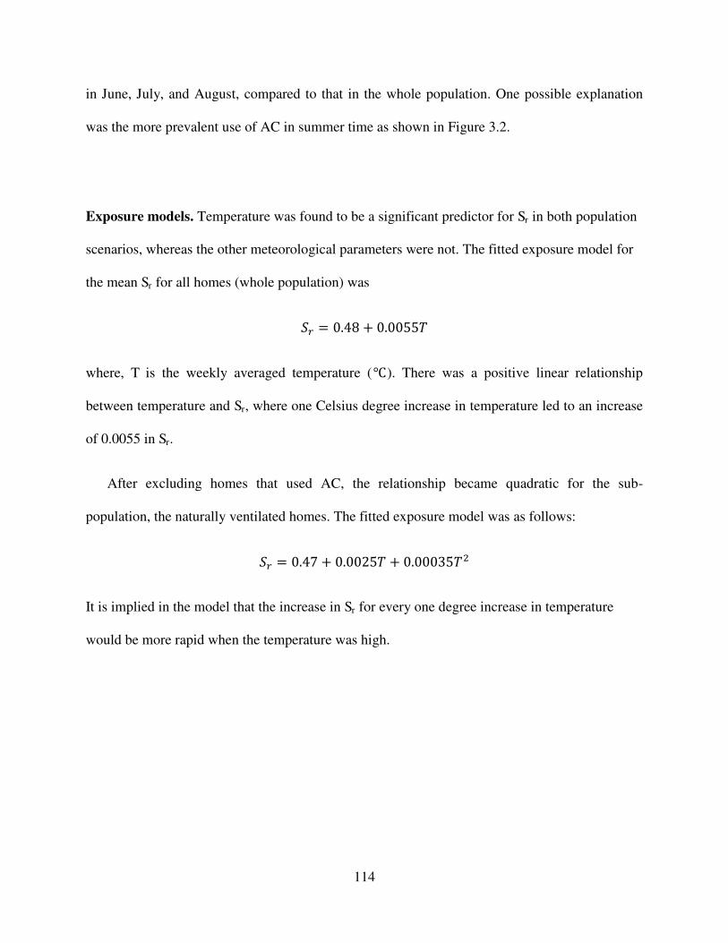
114
in June, July, and August, compared to that in the whole population. One possible explanation
was the more prevalent use of AC in summer time as shown in Figure 3.2.
Exposure models. Temperature was found to be a significant predictor for Sr in both population
scenarios, whereas the other meteorological parameters were not. The fitted exposure model for
the mean Sr for all homes (whole population) was
鯨追 噺 ど┻ねぱ 髪 ど┻どどのの劇
where, T is the weekly averaged temperature (襖). There was a positive linear relationship
between temperature and Sr, where one Celsius degree increase in temperature led to an increase
of 0.0055 in Sr.
After excluding homes that used AC, the relationship became quadratic for the sub-
population, the naturally ventilated homes. The fitted exposure model was as follows:
鯨追 噺 ど┻ねば 髪 ど┻どどにの劇 髪 ど┻どどどぬの劇態
It is implied in the model that the increase in Sr for every one degree increase in temperature
would be more rapid when the temperature was high.
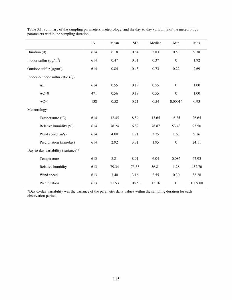
115
Table 3.1. Summary of the sampling parameters, meteorology, and the day-to-day variability of the meteorology parameters within the sampling duration.
N Mean SD Median Min Max
Duration (d) 614 6.18 0.84 5.83 0.53 9.78
Indoor sulfur (g/m3) 614 0.47 0.31 0.37 0 1.92
Outdoor sulfur (g/m3) 614 0.84 0.45 0.73 0.22 2.69
Indoor-outdoor sulfur ratio (Sr)
All 614 0.55 0.19 0.55 0 1.00
AC=0 471 0.56 0.19 0.55 0 1.00
AC=1 138 0.52 0.21 0.54 0.00016 0.93
Meteorology
Temperature (襖岻 614 12.45 8.59 13.65 -6.25 26.65
Relative humidity (%) 614 78.24 6.82 78.87 53.48 95.50
Wind speed (m/s) 614 4.00 1.21 3.75 1.63 9.16
Precipitation (mm/day) 614 2.92 3.31 1.95 0 24.11
Day-to-day variability (variance)*
Temperature 613 8.81 8.91 6.04 0.085 67.93
Relative humidity 613 79.34 73.53 56.81 1.28 452.70
Wind speed 613 3.40 3.16 2.55 0.30 38.28
Precipitation 613 51.53 108.56 12.16 0 1009.00
*Day-to-day variability was the variance of the parameter daily values within the sampling duration for each observation period.
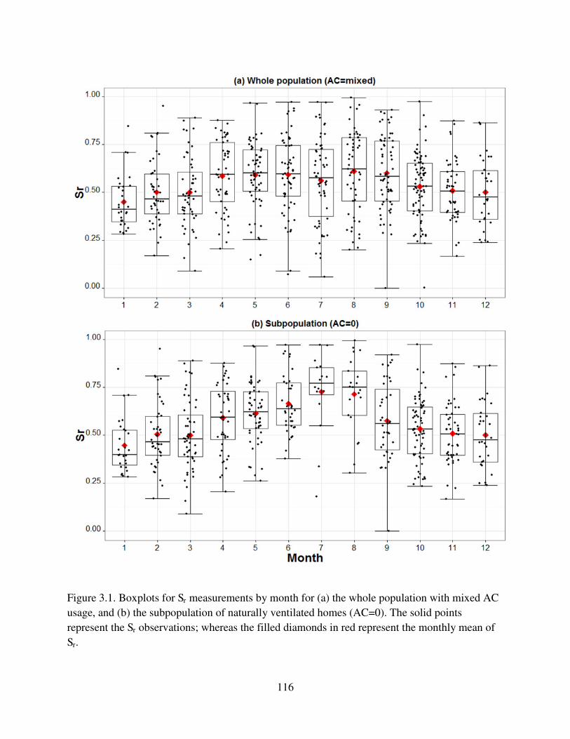
116
Figure 3.1. Boxplots for Sr measurements by month for (a) the whole population with mixed AC
usage, and (b) the subpopulation of naturally ventilated homes (AC=0). The solid points
represent the Sr observations; whereas the filled diamonds in red represent the monthly mean of
Sr.
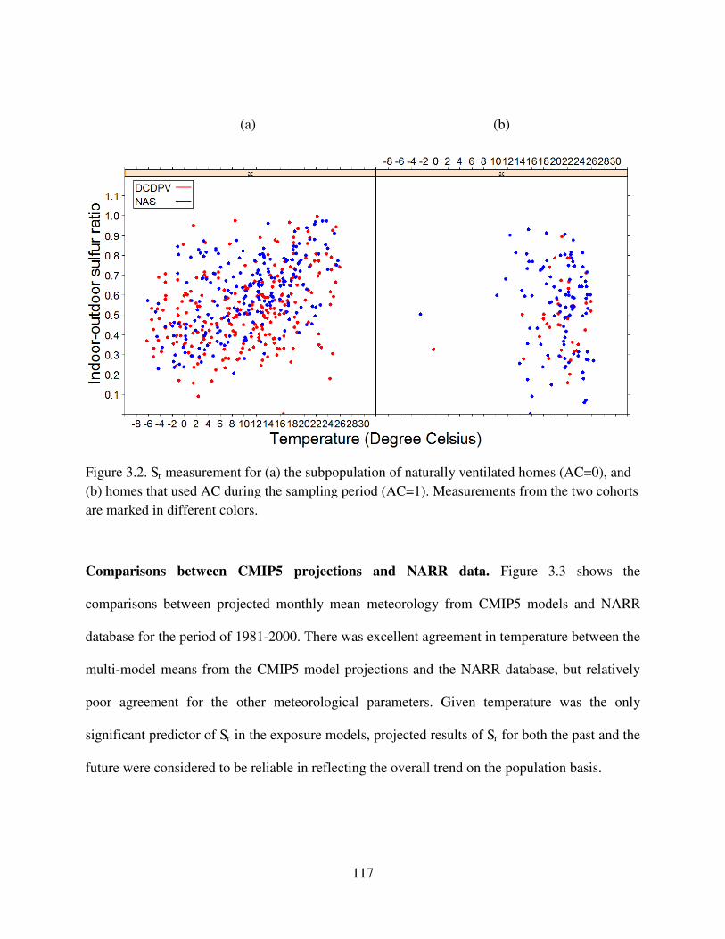
117
(a) (b)
Figure 3.2. Sr measurement for (a) the subpopulation of naturally ventilated homes (AC=0), and
(b) homes that used AC during the sampling period (AC=1). Measurements from the two cohorts
are marked in different colors.
Comparisons between CMIP5 projections and NARR data. Figure 3.3 shows the
comparisons between projected monthly mean meteorology from CMIP5 models and NARR
database for the period of 1981-2000. There was excellent agreement in temperature between the
multi-model means from the CMIP5 model projections and the NARR database, but relatively
poor agreement for the other meteorological parameters. Given temperature was the only
significant predictor of Sr in the exposure models, projected results of Sr for both the past and the
future were considered to be reliable in reflecting the overall trend on the population basis.
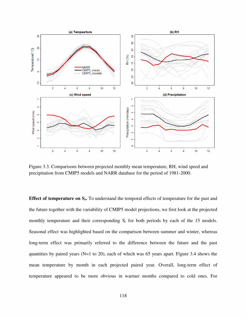
118
Figure 3.3. Comparisons between projected monthly mean temperature, RH, wind speed and
precipitation from CMIP5 models and NARR database for the period of 1981-2000.
Effect of temperature on Sr. To understand the temporal effects of temperature for the past and
the future together with the variability of CMIP5 model projections, we first look at the projected
monthly temperature and their corresponding Sr for both periods by each of the 15 models.
Seasonal effect was highlighted based on the comparison between summer and winter, whereas
long-term effect was primarily referred to the difference between the future and the past
quantities by paired years (N=1 to 20), each of which was 65 years apart. Figure 3.4 shows the
mean temperature by month in each projected paired year. Overall, long-term effect of
temperature appeared to be more obvious in warmer months compared to cold ones. For
119
example, temperature in July was generally warmer in the future, but the increment was harder to
see for January. Conversely, the CMIP5 model variability was larger for winter. As expected, the
trend was exactly the same for the predicted Sr based on the whole population, because Sr had a
linear relationship with temperature (Figure 3.5).
On the other hand, the effect of temperature differed for the subpopulation of naturally
ventilated homes, with quadratic relationship between temperature and Sr (Figure 3.6). A more
rapid increase in Sr was observed in warmer months where CMIP5 model variability was also
higher, compared to winter time. One possible explanation is that the CMIP5 model variability in
the monthly mean temperature was magnified by the quadratic term in the exposure model by
increasingly high temperature.
Finally, the trend of temperature and Sr projections over the 20 year period was relative static
within the same CMIP5 model. We could therefore summarize the estimates into monthly
average across the whole 20 year period, which made it easier to examine the seasonal and long-
term effects of temperature on Sr with CMIP5 model variability.
Seasonal effects. Figure 3.7 shows the 20-year averages of monthly mean temperature for the
future and the past from all 15 CMIP5 models and their overall monthly averages. In general, the
CMIP5 models had good predictability for temperature, where the model-specific trends were
consistent. Variability of the monthly mean across models was more obvious for extreme
temperatures, such as summer and winter. For the future, variability increased in summer. Given
the temperature profiles, the corresponding Sr is displayed in Figure 3.8 for the two populations.
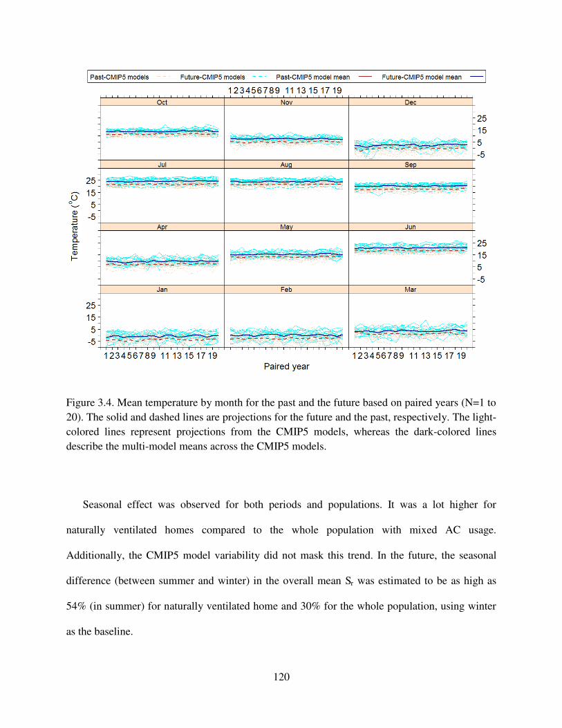
120
Figure 3.4. Mean temperature by month for the past and the future based on paired years (N=1 to
20). The solid and dashed lines are projections for the future and the past, respectively. The light-
colored lines represent projections from the CMIP5 models, whereas the dark-colored lines
describe the multi-model means across the CMIP5 models.
Seasonal effect was observed for both periods and populations. It was a lot higher for
naturally ventilated homes compared to the whole population with mixed AC usage.
Additionally, the CMIP5 model variability did not mask this trend. In the future, the seasonal
difference (between summer and winter) in the overall mean Sr was estimated to be as high as
54% (in summer) for naturally ventilated home and 30% for the whole population, using winter
as the baseline.
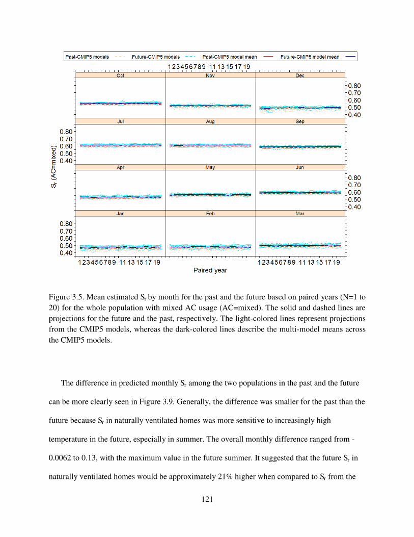
121
Figure 3.5. Mean estimated Sr by month for the past and the future based on paired years (N=1 to
20) for the whole population with mixed AC usage (AC=mixed). The solid and dashed lines are
projections for the future and the past, respectively. The light-colored lines represent projections
from the CMIP5 models, whereas the dark-colored lines describe the multi-model means across
the CMIP5 models.
The difference in predicted monthly Sr among the two populations in the past and the future
can be more clearly seen in Figure 3.9. Generally, the difference was smaller for the past than the
future because Sr in naturally ventilated homes was more sensitive to increasingly high
temperature in the future, especially in summer. The overall monthly difference ranged from -
0.0062 to 0.13, with the maximum value in the future summer. It suggested that the future Sr in
naturally ventilated homes would be approximately 21% higher when compared to Sr from the
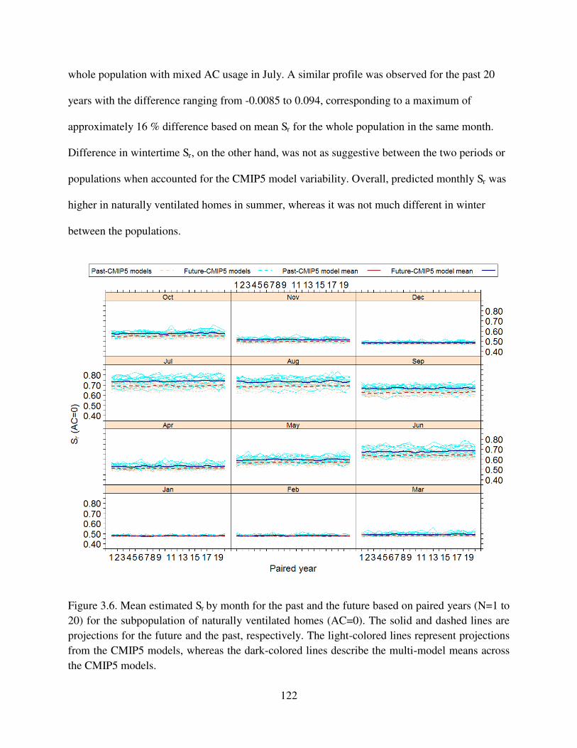
122
whole population with mixed AC usage in July. A similar profile was observed for the past 20
years with the difference ranging from -0.0085 to 0.094, corresponding to a maximum of
approximately 16 % difference based on mean Sr for the whole population in the same month.
Difference in wintertime Sr, on the other hand, was not as suggestive between the two periods or
populations when accounted for the CMIP5 model variability. Overall, predicted monthly Sr was
higher in naturally ventilated homes in summer, whereas it was not much different in winter
between the populations.
Figure 3.6. Mean estimated Sr by month for the past and the future based on paired years (N=1 to
20) for the subpopulation of naturally ventilated homes (AC=0). The solid and dashed lines are
projections for the future and the past, respectively. The light-colored lines represent projections
from the CMIP5 models, whereas the dark-colored lines describe the multi-model means across
the CMIP5 models.
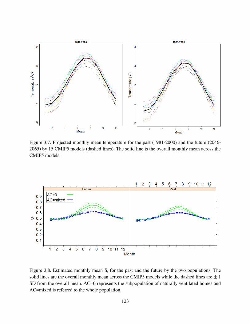
123
Figure 3.7. Projected monthly mean temperature for the past (1981-2000) and the future (2046-
2065) by 15 CMIP5 models (dashed lines). The solid line is the overall monthly mean across the
CMIP5 models.
Figure 3.8. Estimated monthly mean Sr for the past and the future by the two populations. The
solid lines are the overall monthly mean across the CMIP5 models while the dashed lines are 罰 1
SD from the overall mean. AC=0 represents the subpopulation of naturally ventilated homes and
AC=mixed is referred to the whole population.
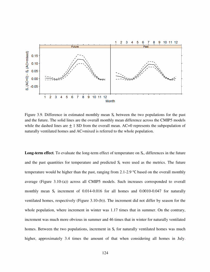
124
Figure 3.9. Difference in estimated monthly mean Sr between the two populations for the past
and the future. The solid lines are the overall monthly mean difference across the CMIP5 models
while the dashed lines are 罰 1 SD from the overall mean. AC=0 represents the subpopulation of
naturally ventilated homes and AC=mixed is referred to the whole population.
Long-term effect. To evaluate the long-term effect of temperature on Sr, differences in the future
and the past quantities for temperature and predicted Sr were used as the metrics. The future
temperature would be higher than the past, ranging from 2.1-2.9 襖 based on the overall monthly
average (Figure 3.10-(a)) across all CMIP5 models. Such increases corresponded to overall
monthly mean Sr increment of 0.014-0.016 for all homes and 0.0010-0.047 for naturally
ventilated homes, respectively (Figure 3.10-(b)). The increment did not differ by season for the
whole population, where increment in winter was 1.17 times that in summer. On the contrary,
increment was much more obvious in summer and 46 times that in winter for naturally ventilated
homes. Between the two populations, increment in Sr for naturally ventilated homes was much
higher, approximately 3.4 times the amount of that when considering all homes in July.
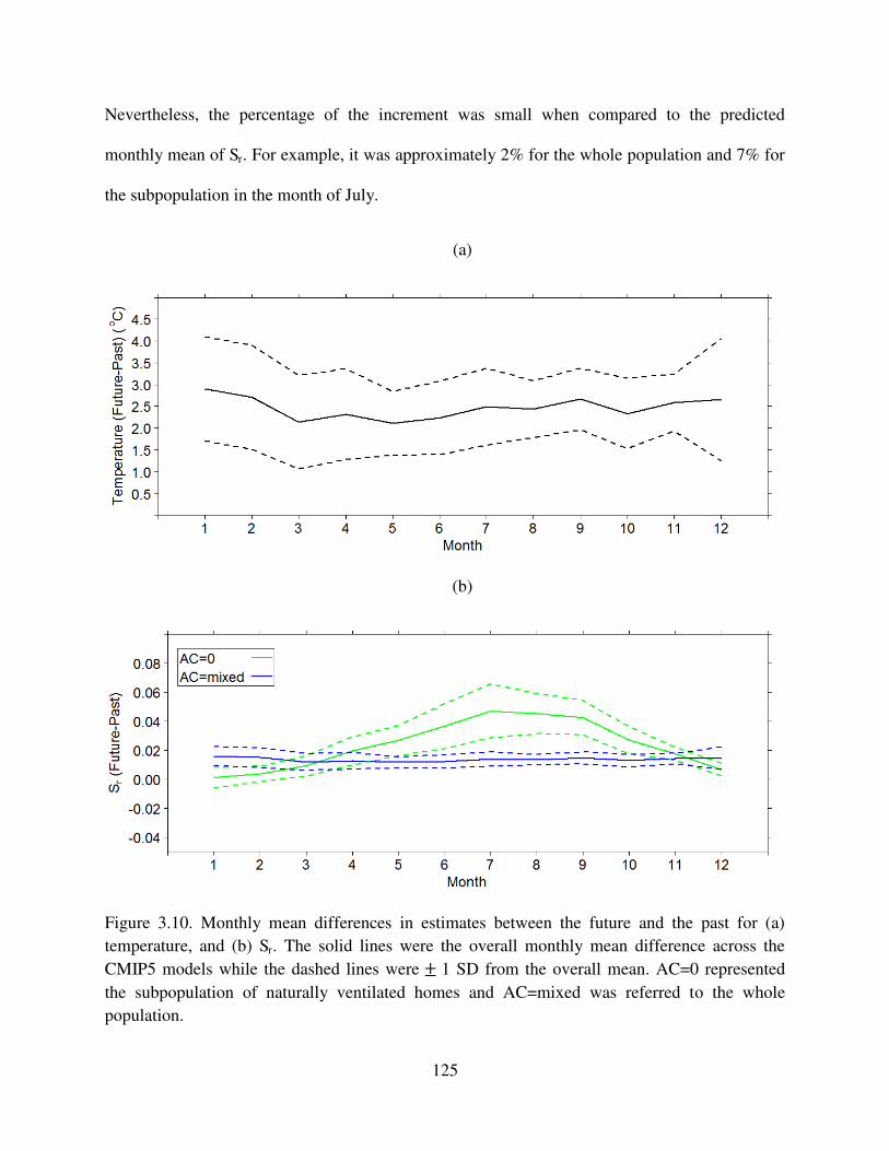
125
Nevertheless, the percentage of the increment was small when compared to the predicted
monthly mean of Sr. For example, it was approximately 2% for the whole population and 7% for
the subpopulation in the month of July.
(a)
(b)
Figure 3.10. Monthly mean differences in estimates between the future and the past for (a)
temperature, and (b) Sr. The solid lines were the overall monthly mean difference across the
CMIP5 models while the dashed lines were 罰 1 SD from the overall mean. AC=0 represented
the subpopulation of naturally ventilated homes and AC=mixed was referred to the whole
population.
126
Discussion
In this study we examined the impact of meteorology on Sr, a surrogate of the outdoor
fraction of indoor PM concentration, with the emphasis on temperature.
Meteorology is known to have strong influences on outdoor PM concentrations. For example,
temperature and absolute humidity possess species-specific effect on PM concentration, mostly
through the competing or additive effect between sulfate, nitrates, and organic aerosols. Higher
temperature increases evaporation of nitrates and organic aerosols, leading to decreased
concentrations. Conversely, it increases sulfate formation through temperature dependent
oxidation process and with more abundant oxidants participating in the reaction (27, 28),
whereas absolute humidity is associated with increase in ammonium nitrate aerosols in summer
due to higher water vapor concentration (27). Wind and precipitation, on the other hand, have
non-species-specific effect on PM concentration. PM are diluted due to higher wind speed or
washed out by higher precipitation (29). However, the resulting temporal or spatial variability
could be high.
To acquire more representative meteorology for the homes in our study cohorts, we matched
the homes to the high resolution data from NARR based on location and sampling period. This
approach aimed to minimize the uncertainty resulting from spatial variability, as opposed to
using data from the central site, on the observed association between meteorology and Sr. We
also accounted for temporal variability by imposing weighting on the association based on the
proportionality of one over variance within the averaged values during each sampling period for
the meteorological parameters. Precipitation was found to have the highest day-to-day
variability. In the final exposure models, temperature was the only significant predictor for Sr,
127
suggesting that the influence of meteorology on Sr was probably not through species-specific PM
properties or their ambient concentrations.
In a study to explore the impact of climate change on indoor air pollution, Nazaroff (30)
classified the influential factors into three categories: properties of pollutants, building factors
(e.g., ventilation), and occupant behavior (e.g., AC usage). Use of AC can decrease the Sr due to
closed windows or/and the filters inside the AC system (31-33). Given the findings of
differential effect of meteorology on Sr in this study, the association between temperature and Sr
was unlikely due to the first category; instead, it could be a result from the last two. We
evaluated the main effect of temperature for the original population with mixed AC usage and
the subpopulation of naturally ventilated homes in the exposure models. It is noteworthy that
adding AC usage as a binary variable (yes or no) in the exposure models was not feasible due to
unbalanced sample size in the binary categories. Additionally, AC was almost exclusively used
in summer, making it impossible to evaluate the effect of temperature that covered such a narrow
temperature range. Separating the exposure models into two populations enabled comparisons of
main effects under different distribution of AC usage. When only considering homes without AC
usage, temperature had a quadratic relationship with Sr, where more rapid increase in Sr was
observed for summer than winter. This could be explained by open windows or doors to ventilate
the house. However, after including the homes that used AC, the differential relationship by
temperature disappeared, particularly for high temperature range. This was because the high Sr
expected for homes with open window in summer were cancelled out by the competing effect
from homes using AC that decreased Sr. This finding not only addresses the impact of AC usage,
but also brings out the importance of population selection when estimating Sr on the population
basis. In our case, the difference in the future Sr can be up to 21 % in July between the
128
populations studied. Therefore, small effects of temperature on Sr in the whole population do not
rule out the health risks for the subpopulation.
The analysis conducted using the selected homes was considered to produce robust
relationships between temperature and Sr. Although the original indoor exposure studies for the
cohorts were not designed to select homes representative of the general population, collectively,
these studies encompass a wide range of homes with different characteristics, collected
throughout the year under varying weather conditions.
We assumed that individuals would react the same way to the same temperature condition
within 65 years, part of which was projected into the future. We also assumed that homes in the
future would be the same as they were 65 years ago. It is possible, however, that homes would be
different in the next 50 years due to advancement in building technology, such as better
insulation, heating, and cooling. But the rate of technology penetration is unknown and depends
on the cost and affordability. On the other hand, the age of homes can vary from a few decades
to 100 or more years, suggesting that it takes a long time to replace homes. Among the 1,151,000
homes surveyed in the greater Boston area in 2007, the median year of structure built was 1951,
where 90% were built before 1985 (34). Since the average monthly temperature was estimated to
change slowly over decades by only 2-3oC, it is reasonable to expect that people would adjust to
climate changes by opening windows more or using more air conditioning in warmer days to
ventilate the house. These changes have the potential to substantially impact home ventilation,
and as a result, the contribution of outdoor sources to total indoor PM2.5, as suggested by the
findings in this study.
129
One limitation of the study was the low temporal resolution of the data, namely weekly
averages of indoor measurements and lack of detailed records on indoor activities. Two potential
issues arise from this limitation. Unavoidably, the multi-day sampling duration included the
intermittent periods of indoor sulfur emission, use of air purifying devices, vacuuming, and other
indoor activities that could potentially violate the MBM assumption and influence the indoor PM
concentration. The interference as anticipated to be larger in the exposure model for the whole
population, where the frequency of AC usage (e.g., number of days in a week) was unknown.
Nevertheless, given some of these activities were routines and limited indoor sulfur sources, the
within home correlation and variability across homes for Sr were expected to be captured in part
by the mixed effects models. Consequently, the exposure models would still give an overall
picture of temperature effect on Sr on a multi-day basis.
The second issue was the insensitivity of the effect estimate to more extreme scenarios, for
example, days of heatwaves. In other words, the day-to-day variability was smoothed by using
integrated samples, leading to smaller effect estimates of temperature in the exposure models.
Nevertheless, we still observed seasonal difference in long-term effect (Figure 3.10-(b)), as well
as long-term difference in seasonal effect of temperature on Sr (Figure 3.9). Although the
increments of overall monthly mean Sr in the future, when based on percentage, were not very
large, they could deviate from but still center around the observed monthly mean Sr values when
daily data are available. Consequently, it remains inconclusive whether climate change would
impact Sr significantly and thus modify the effect of PM on health, especially in vulnerable
populations.
Another limitation of the study was the lack of information of to what extent did the home
environment meet the steady state assumption of the MBM over the sampling period. The multi-
130
day sampling duration could introduce certain variability in the steady state situation, as
described above. In Chapter 2, we know that under relatively well-mixed environment, the MBM
could be applied to estimate the indoor PM concentrations as a function of outdoor PM
concentration, air exchange rate, particle penetration coefficient, particle deposition rate, and
filtration parameters in a given space. Validation of the assumption is not feasible in large-scaled
home studies; nevertheless, the steady state approach has been used in many studies to determine
those parameters (6, 21, 35-37). Based on the assumption, we were able to estimate the
corresponding parameters in the MBM with measured Sr, which is of great contribution to the
modeling application in estimating PM exposure from a large number of homes.
A unique strength of the study is that we were the first to explore the relationship between
monthly and long-term temperature change and Sr on the population basis, with capitalizing on
an assembly of a large number of home measurements. Our results projecting changes in the
relative temporal contribution of temperature to indoor exposure to outdoor PM are valuable for
future assessments and providing implications in possible intervention. We found that Sr was
independent of meteorology studied, with the exception of temperature. Monthly effect of
temperature, highlighted by summer-winter difference, was much more dominant when
compared to long-term effect on Sr, which differed in the two populations. PM2.5 exposure was
high in summer, especially in naturally ventilated homes. AC, air purifying devices and/or closed
window status could be potentially effective interventions for reducing indoor PM exposure,
based on the comparison of Sr between the two populations in this study, and the findings from
the previous chapter.
Finally, as discussed in the previous paragraphs, findings from the study can be utilized to
evaluate the relevant parameters influencing indoor PM concentrations in the study homes, such
131
as particle penetration coefficient and deposition rate, which in turn helps determine the indoor
source contribution. More importantly, when given the data of future outdoor PM concentrations,
Sr can be used to independently estimate the outdoor fraction of indoor PM, regardless various
indoor sources. It can subsequently be applied to further assess the modification of Sr on the
relationship between future indoor PM exposure and public health in the greater Boston area.
In the future, the study method can be applied to assess the effect of temperature on Sr in
other cities of distinct weather conditions, building characteristics and occupant behaviors, where
Boston can be used as reference city for comparison.
132
Bibliography
(1) Lim, S.S.; Vos, T.; Flaxman, A.D.; Danaei, G.; Shibuya, K.; Adair-Rohani, H. A comparative
risk assessment of burden of disease and injury attributable to 67 risk factors and risk factor
clusters in 21 regions, 1990–2010: a systematic analysis for the Global Burden of Disease Study
2010. The lancet 2013, 380 (9859), 2224-2260.
(2) Klepeis, N.; Nelson, W.; Ott, W.; Robinson, J.; Tsang, A.; Switzer, P.; Behar, J.; Hern, S.;
Engelmann, W. The National Human Activity Pattern Survey (NHAPS): a resource for assessing
exposure to environmental pollutants. J. Expo. Anal. Environ. Epidemiol. 2001, 11 (3), 231-252;
10.1038/sj.jea.7500165.
(3) Meng, Q.Y.; Turpin, B.J.; Korn, L.; Weisel, C.P.; Morandi, M.; Colome, S. Influence of
ambient (outdoor) sources on residential indoor and personal PM2. 5 concentrations: analyses of
RIOPA data. Journal of Exposure Science and Environmental Epidemiology 2005, 15 (1), 17-28.
(4) Liu, D. and Nazaroff, W.W. Particle Penetration Through Building Cracks. Aerosol Science
and Technology 2003, 37, 565-573.
(5) Thatcher, T.L. and Layton, D.W. Deposition, resuspension, and penetration of particles
within a residence. Atmospheric Environment 1995, 29 (13), 1487-1497.
(6) Long, C.M.; Suh, H.H.; Catalano, P.J.; Koutrakis, P. Using time- and size-resolved
particulate data to quantify indoor penetration and deposition behavior. Environ. Sci. Technol.
2001, 35 (10), 2089-2099; 10.1021/es001477d.
133
(7) Chen, C.; Zhao, B.; Weschler, C.J. Indoor exposure to “outdoor PM10”: assessing its
influence on the relationship between PM10 and short-term mortality in US cities. Epidemiology
2012, 23 (6), 870-878.
(8) Hodas, N.; Meng, Q.; Lunden, M.M.; Rich, D.Q.; Özkaynak, H.; Baxter, L.K. Variability in
the fraction of ambient fine particulate matter found indoors and observed heterogeneity in
health effect estimates. Journal of Exposure Science and Environmental Epidemiology 2012, 22
(5), 448-454.
(9) Bell, M.L. and Dominici, F. Effect modification by community characteristics on the short-
term effects of ozone exposure and mortality in 98 US communities. American journal of
epidemiology 2008, 167 (8), 986-997.
(10) Levy, J.I.; Chemerynski, S.M.; Sarnat, J.A. zone exposure and mortality: an empiric bayes
metaregression analysis. Epidemiology 2005, 16 (4), 458-468.
(11) Janssen, N.A.; Schwartz, J.; Zanobetti, A.; Suh, H.H. Air conditioning and source-specific
particles as modifiers of the effect of PM (10) on hospital admissions for heart and lung disease.
Environmental health perspectives 2002, 110 (1), 43.
(12) Medina-Ramón, M.; Zanobetti, A.; Schwartz, J. The effect of ozone and PM10 on hospital
admissions for pneumonia and chronic obstructive pulmonary disease: a national multicity study.
American journal of epidemiology 2006, 163 (6), 579-588.
134
(13) Sarnat, J.A.; Sarnat, S.E.; Flanders, W.D.; Chang, H.H.; Mulholland, J.; Baxter, L.
Spatiotemporally resolved air exchange rate as a modifier of acute air pollution-related morbidity
in Atlanta. Journal of Exposure Science and Environmental Epidemiology 2013, 23 (6), 606-615.
(14) Wallace, L.A.; Emmerich, S.J.; Howard-Reed, C. Continuous measurements of air change
rates in an occupied house for 1 year: the effect of temperature, wind, fans, and windows.
Journal of exposure analysis and environmental epidemiology 2002, 12 (4), 296-306.
(15) Kearney, J.; Wallace, L.; MacNeill, M.; Héroux, M.E.; Kindzierski, W.; Wheeler, A.
Residential infiltration of fine and ultrafine particles in Edmonton. Atmospheric Environment
2014, 94, 793-805.
(16) Chan, W.R.; Price, P.N.; Nazaroff, W.W.; Gadgil, A.J. Distribution of residential air
leakage: Implications for health outcome of an outdoor toxic release. Indoor air 2005, 15 (11),
1729-1734.
(17) Persily, A.; Musser, A.; Emmerich, S.J. Modeled infiltration rate distributions for US
housing. Indoor air 2010, 20 (6), 473-485.
(18) Sherman, M.H. and Chan, W.R. Building air tightness: research and practice. Building
Ventilation: the state of the Art 2006, , 137-162.
(19) Diapouli, E.; Chaloulakou, A.; Koutrakis, P. Estimating the concentration of indoor particles
of outdoor origin: A review. Journal of the Air & Waste Management Association 2013, 63 (10),
1113-1129.
135
(20) Hoxha, M.; Dioni, L.; McCracken, J.P.; Baccarelli, A.; Melly, S.J.; Coull, B.A. Annual
ambient black carbon associated with shorter telomeres in elderly men: Veterans Affairs
Normative Aging Study. Environmental health perspectives 2010, 118 (11), 1564-1570.
(21) Sarnat, J.A.; Long, C.M.; Koutrakis, P.; Coull, B.A.; Schwartz, J.; Suh, H.H. Using sulfur
as a tracer of outdoor fine particulate matter. Environmental Science & Technology 2002, 36
(24), 5305-5314.
(22) Chuang, K.J.; Coull, B.A.; Zanobetti, A.; Suh, H.; Schwartz, J.; Stone, P.H. Particulate air
pollution as a risk factor for ST-segment depression in patients with coronary artery disease.
Circulation 2008, 118 (13), 1314-1320.
(23) Baja, E.S.; Schwartz, J.D.; Wellenius, G.A.; Coull, B.A.; Zanobetti, A.; Vokonas, P.S.; Suh,
H.H. Traffic-related air pollution and QT interval: modification by diabetes, obesity, and
oxidative stress gene polymorphisms in the normative aging study. Environmental health
perspectives 2010, 118 (6), 840-846.
(24) NCEP North American Regional Reanalysis (NARR) .
(25) Stocker, T.F.; Qin, D.; Plattner, G.K.; Tignor, M.; Allen, S.K.; Boschung, J.
Intergovernmental panel on climate change, working group I contribution to the IPCC fifth
assessment report (AR5). 2013, .
(26) Moss, R.H.; Edmonds, J.A.; Hibbard, K.A.; Manning, M.R.; Rose, S.K.; Van Vuuren, D.P.
The next generation of scenarios for climate change research and assessment. Nature 2010, 463
(7282), 747-756.
136
(27) Seinfeld, J.H. and Pandis, S.N. Atmospheric chemistry and physics: from air pollution to
climate change. John Wiley & Sons 2012, .
(28) Sweet, C.W. and Gatz, D.F. Summary and analysis of available PM 2.5 measurements in
Illinois. Atmospheric Environment 1998, 32 (6), 1129-1133.
(29) Dawson, J.P.; Adams, P.J.; Pandis, S.N. Sensitivity of PM 2.5 to climate in the Eastern US:
a modeling case study. Atmospheric chemistry and physics 2007, 7 (16), 4295-4309.
(30) Nazaroff, W.W. Exploring the consequences of climate change for indoor air quality.
Environmental Research Letters 2013, 8 (1), 015022.
(31) Howard-Reed, C.; Wallace, L.A.; Emmerich, S.J. Effect of ventilation systems and air
filters on decay rates of particles produced by indoor sources in an occupied townhouse. Atmos.
Environ. 2003, 37 (38), 5295-5306; 10.1016/j.atmosenv.2003.09.012.
(32) Sarnat, J.A.; Koutrakis, P.; Suh, H.H. Assessing the relationship between personal
particulate and gaseous exposures of senior citizens living in Baltimore, MD. Journal of the Air
& Waste Management Association 2000, 50 (7), 1184-1198.
(33) Wallace, L. and Howard-Reed, C. Continuous monitoring of ultrafine, fine, and coarse
particles in a residence for 18 months in 1999-2000. . Journal of the Air & Waste Management
Association 2002, 52 (7), 828-844.
(34) U.S. Census Bureau American Housing Survey for the. Boston Metropolitan Area: 2007.
137
(35) Abt, E.; Suh, H.H.; Catalano, P.; Koutrakis, P. Relative contribution of outdoor and indoor
particle sources to indoor concentrations. Environ. Sci. Technol. 2000, 34 (17), 3579-3587;
10.1021/es990348y.
(36) Wallace, L. and Williams, R. Use of personal-indoor-outdoor sulfur concentrations to
estimate the infiltration factor and outdoor exposure factor for individual homes and persons.
Environmental science & technology 2005, 39 (6), 1707-1714.
(37) Hodas, N.; Meng, Q.; Lunden, M.M.; Turpin, B.J. Toward refined estimates of ambient PM
2.5 exposure: Evaluation of a physical outdoor-to-indoor transport model. Atmospheric
Environment, 2014, 83, 229-236.

138
CONCLUSIONS
139
In the preceding chapters we discussed in each study the challenges that motivated the
objectives, limitations of the study design, and implications from the findings. In this chapter, I
would like to summarize the major findings from the presented work and shed light on both the
innovation and limitations, based on which I suggested future directions.
In Chapter 1, we estimated the size-resolved particle deposition rates for the ultrafine and
submicrometer particles during non-sourced period following a controlled sourced period in a
well-mixed residential environment inside an apartment. The study design in conjunction with
the non-linear mixed effects modeling procedure provided a feasible and alternative method for
estimating particle deposition rates when the background concentration cannot be measured. A
dynamic adjustment method with constant injection of tracer gas was used to maintain the air
exchange rate at three target levels: 0.60, 0.90 and 1.20 h-1, as the sampling conditions.
Particle deposition was found to be highly size dependent with rates ranging from 0.68 ±
0.10 to 5.03 ± 0.20 h-1 (mean ± SE). While acknowledging the large variability in the size-
resolved deposition rates reported from the previous studies and considering the relatively small
95% confidence intervals for the mean estimates of 倦沈 in this study, we found that our estimates
for submicrometer particles were in close agreement with some of these studies. However, the
mean estimates of deposition rate for the ultrafine particles were considerably higher than the
reported deposition rates from the others, which could possibly be explained by the effect of
enhanced air mixing by the operation of portable fans. The effect of air exchange on the particle
deposition under enhanced air mixing was relatively small when compared to both the strong
influence of size-dependent deposition mechanisms and the effects of mechanical air mixing by
fans. Nonetheless, the significant association between air exchange and particle deposition rates
for a few size categories indicated potential influence of air exchange on particle deposition.
140
In Chapter 2, as a companion study, we validated the use of the MBM to determine the
effectiveness of portable air purifiers in removing ultrafine and submicrometer particles in the
same apartment. We evaluated two identical portable air purifiers, equipped with high efficiency
particulate air filters, for their performance under three different air flow settings and three target
air exchange rates. We subsequently used a mixed effects model to estimate the slope between
the measured and modeled effectiveness by particle size. Similar to the findings in Chapter 1,
effectiveness was highly particle size-dependent. For example, at the lowest target air exchange
rate, it ranged from 0.33 to 0.56, 0.51 to 0.75, and 0.60 to 0.81 for the three air purifier flow
settings, respectively. Our findings suggested that filtration was the dominant removal
mechanism for submicrometer particles, whereas deposition could play a more important role in
ultrafine particle removal. We found reasonable agreement between measured and modeled
effectiveness with size-resolved slopes ranging from 1.11 ± 0.06 to 1.25 ± 0.07 (mean ± SE),
except for particles <35 nm.
In Chapter 3, we assembled data from two cohorts in the greater Boston area, assessing the
monthly and long-term effect of temperature and other meteorology on Sr, a surrogate of
infiltration factor for PM2.5 in two populations: the whole population with mixed AC usage and
the subpopulation of naturally ventilated homes. We found that Sr was independent of
meteorology studied, with the exception of temperature. Monthly effect of temperature,
highlighted by summer-winter difference, was much more dominant when compared to long-
term effect on Sr, which differed in the two populations. In the future, the seasonal difference
(between summer and winter) in Sr was estimated to be as high as 54% for naturally ventilated
home and 30% for the whole population, using winter as the baseline. The overall monthly
difference ranged from -0.0062 to 0.13, with the maximum value in the future summer. It
141
suggested that the future Sr in naturally ventilated homes would be approximately 20% higher
when compared to Sr from the whole population with mixed AC usage in summer. Overall,
predicted monthly Sr was higher in naturally ventilated homes in summer, whereas there was no
population difference in winter.
Overall, the future temperature was higher than the past, ranging from 2.1-2.9 襖 based on
the monthly average. Such increases corresponded to monthly Sr elevation of 0.014-0.016 for all
homes and 0.0010-0.047 for naturally ventilated homes, respectively (Figure 3.8). The elevation
did not differ by season for the whole population, where increment in winter was 1.17 times that
in summer. On the contrary, increment was much more obvious in summer and was 46 times that
in winter for naturally ventilated homes. Between the two populations, increment in Sr for
naturally ventilated homes was much higher, approximately 3.4 times the amount of that when
considering all homes in July. Nevertheless, the percentage of the increment was small when
compared to the predicted monthly mean of Sr. For example, it was approximately 2% for the
whole population and 7% for the subpopulation in the month of July. In sum, we observed
seasonal difference in long-term effect (Figure 3.10-(b)), as well as long-term difference in
seasonal effect of temperature on Sr (Figure 3.9).
Study limitation is often a two sided sword, with one aspect of attenuating the interpretability
of the current study findings, while indicating future directions to fill the existing gaps. One
major limitation in the single-home study was the enhanced air mixing to achieve well-mixed
environment. As an initial investigation and implementation of the study approach, it was
reasonable yet unavoidable, to start from the most conservative scenario with least deviation
from the model assumptions. Results can provide us insight for future work and overcome the
existing limitations. For example, we would be interested in exploring how air mixing conditions
142
influence size-resolved particle deposition rate and PAP effectiveness in terms of spatial and
temporal concentration distribution of indoor PM, by varying fan speeds. The same approach can
be used to study the effect of air exchange on particle deposition as well.
The major limitation in the multi-home observational study was lack of high temporal
resolution data, leading to interference from intermittent indoor sources or more variable
combination of activities that violates MBM assumptions, and small effect estimate of
temperature. However, given daily data in the future, we expect to more sensitively detect effects
of meteorology on Sr and to be able to estimate particle deposition rate and penetration
coefficient with known air exchange rate values.
Both the single-home and multi-home observational studies have original components that
are pioneering and innovative in their specific fields of study. One important merit shared by
these research designs and structures, however, is that they can be replicated in various
residential settings, or in observational studies with distinct temporal or spatial features, such as
outside of the greater Boston area.
To our knowledge, the home study in Chapter 1 and 2 was the first to validate the steady
state MBM for predicting the size-resolved effectiveness of PAPs in a residential setting. The
study design and approach for establishing an environment that met the MBM assumptions were
ambitious but successful, making it possible to estimate size-resolved deposition rate, validate
the use of MBM in a home, and assess the effectiveness of PAPs with minimized uncertainties
from violation of assumption. The design and the corresponding approach featured the
achievement of a well-mixed indoor environment using portable fans, the generation of artificial
particles at a constant rate to substantially elevate indoor concentration to minimize the
143
interference from the variability of outdoor PM, and the use of a dynamic method to maintain air
exchange rates at constant levels throughout the sampling period. The same approach can further
be applied to understand other particle behaviors in the future. For example, given simultaneous
ambient PM measurement outside of the house, we can estimate the penetration coefficient via
non-linear mixed effects model. Although this type of controlled home experiments with size-
resolved data acquisition is not feasible for large-scale home studies, increasing amount of data
collection using selected homes with various characteristics can still improve generalizability
and representativeness of the collective measurements. Indoor PM exposure can be subsequently
estimated or predicted based on the known values of model parameters with improved
confidence in data interpretation. Precautionary measures or actions of intervention can then be
suggested to reduce particle exposure in homes.
Similarly, a unique strength of the study in Chapter 3 is that we were the first to explore the
relationship between monthly and long-term temperature change and Sr on the population basis,
with capitalizing on an assembly of a large number of home measurements. Discussion of
meteorology effect from other studies is often limited by incomplete cycle of seasons and the
number of samples. Our database consists a large number of measurements and homes that were
sampled through all seasons, meanwhile covering various building characteristics. Furthermore,
data on occupant behavior such as window opening was relatively balanced across the
temperature range studied. Additionally, we matched study homes to the NARR database by
location and sampling date, minimizing uncertainties due to spatial variability of meteorology
when compared to the conventional approach of using meteorology data from the central site.
We also reported monthly mean Sr with CMIP5 model variability to demonstrate potential
uncertainties in Sr prediction from weather projection. With the progressing development of the

144
CMIP models, reliability in meteorology prediction are expected to increase with uncertainties
better explained, contributing to more refined Sr predictions. In the future, the study method can
be applied to assess the effect of temperature on Sr in other cities of distinct weather conditions,
building characteristics and occupant behaviors, where Boston can be used as the reference city
for comparison.
When viewed together, understandings of the physical mechanisms in the first two chapters,
such as size-resolved particle deposition behavior, PAP effectiveness and reliability of MBM
applications, can be used to explain, in part, the observed association between meteorology and
Sr in the third chapter, especially with available daily observations in the future. As a result,
findings from this dissertation not only intertwine in the causal framework of linking human
exposure to indoor PM and the related health risks, but also contribute to more comprehensive
exposure assessment. By assessing the mass balance application inside out, we could envision
future researches in exploring roles of various mechanisms and interventions in reducing indoor
PM exposure, eventually improving our knowledge on the development of strategies to protect
public health.