Second International Symposium on Marine Propulsors smp’11, Hamburg, Germany, June 2011

From Single to Multistage Marine Propulsor: A Fully Numerical Design Approach

Stefano Gaggero1, Davide Grassi

2, Stefano Brizzolara

1

1Marine CFD Group, Department of Naval Architecture, Marine and Electrical Engineering, University of Genova, Italy.

2ZF Marine Group, Arco di Trento, Italy.

ABSTRACT

The limitations of classical theories for the design of

contra-rotating propellers suggest the necessity to develop

fully numerical procedures to address designs with

different front/rear rotational speed and/or number of

blades, as well as unbalanced distributions of thrust

between the propellers and the presence of hub and ducts.

The present paper compares the design of a couple of

contra-rotating propellers carried out by a classical

Morgan-Lerbs approach and a fully numerical procedure

based on a variational approach (Coney 1989) for the

bounded circulation. Results in terms of circulation

distribution, self-induced velocities and blade geometry

are presented. Three different analysis tools, a lifting

surface, a panel method and a RANS solver are finally

applied to analyze the hydrodynamic performance of the

generated designs in order to validate the design

approach. It will be shown that the propellers designed

with the two proposed approaches satisfy the design

requirements as confirmed by all the three analysis

methods. Moreover, it will be stated that the balanced

load solution is the more efficient.

Keywords

Contra-Rotating Propellers, Propeller Design, RANS,

Panel Method, Lifting Surface.

1 INTRODUCTION

Contra-rotating propellers have been widely used for

decades in outboard propulsion units for fast-planing craft

or in podded drives for fast ships or mega-yachts due to

its advantage in terms of overall propulsive efficiency,

mechanical balance and shallow draft (an important issue,

in particular for pleasure boats). By splitting the thrust

and torque between the fore and the aft propeller, the

expanded area ratio and the diameter can be reduced,

keeping the same cavitation margin when compared to a

classical single propeller solution. However, the potential

application of contra-rotating propellers is really wide,

also being suitable for large displacement ship in

conventional shaft line arrangement. The present paper

deals with comparison between two different design

approaches and three analysis tools; a set of contra-

rotating propellers for podded drives has been designed

through a classical lifting-line theory and a fully

numerical lifting-line approach; and then the resulting

geometries have been analyzed via a lifting-surface code,

a panel code and commercial RANS tool in order to

compare performances in terms of thrust/torque curves

and induced velocities. The classical lifting-line approach

is based upon the Morgan-Lerbs theory for calculating

optimum blade circulation with some additional features

like the numerical treatment of the induced velocities, the

possibility to unload the optimum blade circulation at tip

and hub radial positions and a fully automated blade

geometry optimization for cavitation and strength

assessment. While the foregoing method assumes a

thrust/torque balance between the front and aft propeller

and does not take into account for any hub effects, the

fully numerical design approach solve a Lagrange

multiplier minimization problem allowing for different

load distribution and modelling the presence of the hub.

For the analysis, a lifting surface (Grassi & Brizzolara

2009) and a panel (Gaggero & Brizzolara 2009) code,

both developed for single propellers, have been modified

in order to account for multi-stage propulsor, following an

iterative approach and solving each propeller as a single

one in a wake-adapted condition where the inflow

velocity is calculated by solving the other propeller.

Moreover, in order to solve both the propellers together, a

RANS commercial solver has been used following a

quasi-steady and a fully unsteady approach

The former RANS solution approach allows for a fast

averaged solution of the contra-rotating propeller set, each

operating in a time constant inflow wake. In this sense,

the quasi-steady approach is similar to the iterative

approach based on the mean inflow, adopted for the

analysis of the contra-rotating propellers by the potential

flow based methods. On the other hand, the RANS fully

unsteady solution allows to compute the unsteady effects

related to the time varying relative positions between

front and rear propellers and to have a better insight into

the hydrodynamic phenomena that characterize contra-

rotating propellers.

2 DESIGN PROCEDURE

As mentioned before, the present work uses two different

approaches for determining the optimum blade

circulation, whereas a common method (see Chapter 2.3)

is adopted for generating the blade shape.

2.1 Revised Morgan-Lerbs Approach

The first design approach (Brizzolara et al 2008) is based

upon a revisited Morgan-Lerbs theory (Morgan et al

1960). The design theory describing contra-rotating

propeller is more complicated with respect to that for the

single case, due to the interference between the propellers

itself; for this reason, some simplifying assumptions are

needed in order to come to a partially analytical solution

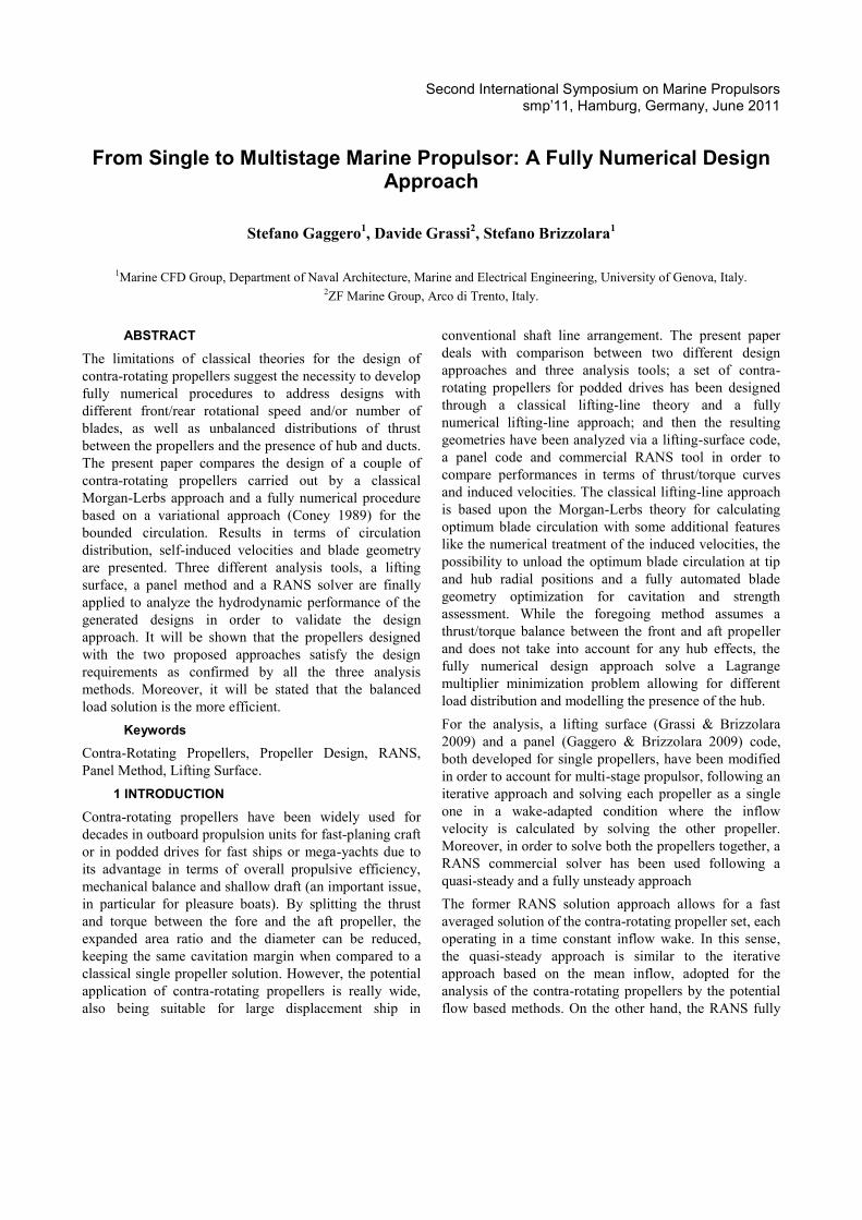
of the mathematical problem. The velocity diagram for

fore and aft propeller is depicted in Figure 1.

Figure 1: Induced velocities for the Morgan-Lerbs

approach.

Under some assumption regarding the induced velocities

that comes from the momentum theory, Morgan derives

the following relationship between self-induced and

interference velocities:

( ) ( ) ( ) [ ( ) ]

( )

( ) ( ) ( ) [ ( ) ]

( ) ( ) ( ) [ ( ) ]

(1)

Where subscripts 1 means at forward propeller, 2 means

at rear propeller, a stands for axial, t for tangential

component, s for self-induced and i for interference

induced components of velocity.

The key point lays in the definition of the so-called

“Equivalent Propeller”, i.e., the optimum propeller which

produces 50% of the required thrust and absorbs 50% of

the total torque, having the hydrodynamic pitch angle

equal to the average of the hydrodynamic pitch angles of

the actual propellers. In other words, at a first step Lerbs‟s

method assumes that the longitudinal distance between

the propellers is zero (props are infinitely close together),

so that the mutual induced velocities become independent

from the propeller longitudinal distance, being a function

of bound circulation and induction factor given by the

classical Lerbs theory for single wake adapted propellers.

Moreover, since unsteady effect is not taken into account,

some factors, and , for obtaining a circumferential

average of the mutual induced velocities are introduced.

As mentioned in the introduction, the present theory

offers the possibility of imposing a circulation distribution

(which differs from the optimum one) in order to unload

the blade, especially near tip and root sections; this

feature is addressed by applying Lerbs‟s non-optimum

lifting line theory to the Equivalent Propeller with some

corrections in order to treat the peculiarities of the contra-

rotating case. An unloading factor (function of the

radial position) is applied to the total circulation (expressed as a sum of n odd sinusoidal function), so

obtaining the new modified total circulation :

∑

( )

(2)

Where is related to the nondimensional radius

through the following equation:

( )

( ) (3)

Such a modified circulation is then scaled by a factor in

order to develop the prescribed thrust. A final unloaded

circulation is so derived as follows:

(4)

The foregoing procedure for unloading the blade

circulation will also be applied to the fully numerical

approach described later. Once the circulation for the

Equivalent Propeller is derived, the next design stage is to

calculate the hydrodynamic pitch for the actual propeller

by introducing some longitudinal interference factors,

and (being function of distance, radial position and

propeller loading). As mentioned in the introduction, a

completely numerical lifting-line method has been

developed to calculate circumferential and longitudinal

interference factors. The lifting-line model is similar to

that of Lerbs (1952), but it has been changed from a

continuous formulation into a discrete one by employing

vortex lines composed by constant length parts. So,

induced velocities are not evaluated by the well-known

analytical formulations, but by simply applying the Biot-

Savart law to the discrete bound vortex elements and to

the free trailing vortices.

2.2 Fully Numerical Approach

The fully numerical design approach for contra-rotating

propeller is based on the original idea of Coney (1989) for

the definition of optimum radial circulation distribution

for lightly and moderately loaded propeller in non-

uniform inflow. Traditional lifting-line approaches are, as

presented above, mainly based on Betz criteria for the

minimum energy loss on the flow downstream of the

propeller. The satisfaction of these conditions is realized

by an optimum circulation distribution, generally defined

as a sinus series over the blade span. In the fully

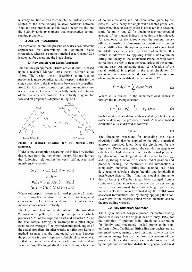
numerical design approach, this continuous distribution of

vorticity along the lifting line representing each constant

angular spaced blade of the propeller is discretized with a

lattice of vortex elements of constant strength. The

continuous trailing vortex sheet that represent the blade

trailing wake is therefore replaced by a set M of vortex

horseshoes of intensity ( ), each composed by two

helical trailing vortices and a bound vortex segment on

the propeller lifting line, as in Figure 2. Also, the

propeller hub effect can be included by means of image

vortices based on the well-known principle that a pair of

two-dimensional vortices of equal and opposite strength,

located on the same line, induce no net radial velocity on

a circle of radius rh:

(5)

where r is the radius of the outer vortices, ri the radius of

its image and rh the radius of the hub cylinder. The same

result approximately holds in the case of three

dimensional helical vortices, provided that their pitch is

sufficiently high.

This system of discrete vortex segments, bound to the

lifting line or part of each helical vortex line trailed in the

wake (Figure 2) induces axial and tangential velocity

components on each control points of the lifting line.

These self-induced velocities are computed applying the

Biot-Savart law, in such a way:

( ) ( ) ∑ ( )

( ) ( ) ∑ ( )

(6)

where Aim and Tim are, as usual, the axial and tangential

velocity influence coefficients of a unit horseshoe vortex

placed at the m-radial position on the i-control point on

the lifting line, and M and Mh are the total number of

horseshoe vortices on the blade and on the image hub.

With this discrete model, the hydrodynamic thrust and

torque characteristics of the propeller can be computed by

adding the contribution of each discrete vortex on the

line. In fact, under the assumption of pure potential and

inviscid flow:

∫

∫

(7)

where is simply the total tangential velocity

acting at the lifting line (inflow plus self induced plus rotational tangential velocity ), is the

axial velocity (inflow plus self induced axial velocity

), and is the local angle of attack. In discrete form,

equation (3) can be expressed as:

∑[ ( ) ( )] ( )

∑[ ( ) ( )] ( )

(8)

A variational approach provides a general procedure to

identify a set of discrete circulation values ( ) (i.e., the

radial circulation distribution for each propeller blade)

such that the torque (as computed in Equation (3)) is

minimized subjected to the constraint that the thrust must

satisfy the prescribed value .

Figure 2: Discretized lifting line and reference system.

Introducing the additional unknown represented by the

Lagrange multiplier , the problem can be solved in terms

of an auxiliary function ( ) requiring

that its partial derivatives are zeros:

( )

(9)

Carrying out the partial derivatives, Equation (9) leads to

a nonlinear system of equations for the vortex strengths

and for the Lagrange multiplier. The iterative solution of

the nonlinear system is obtained by the linearization

proposed by Coney (1989) in order to achieve the optimal

circulation distribution. This formulation can be further

improved to design moderately loaded propeller and to

include viscous effects. The initial horseshoe vortexes

that represent the wake, frozen during the solution of

Equation (9), can be aligned with the velocities induced

by the actual distribution of circulation and the solution

iterated again until convergence of the wake shape (or of

the induced velocities themselves). A viscous thrust

reduction, as a force acting on the direction parallel to the

total velocity and thus as a function of the self-induced

velocities themselves, can be added to the auxiliary

function ; and a further iterative procedure, each time

the chord distribution of the propeller has been

determined, can be set. In total, for the design of a single

propeller, the devised procedure works with:

An inner-iterative approach for the determination

of the optimal circulation distribution,

A second-level iterative approach to include the

viscous drag on the optimal circulation

distribution,

A third-level iterative approach to include the

wake alignment and the moderately loaded case.

Contra-rotating propellers requires an equivalent

approach, defining an auxiliary function as a combination

of thrust and torque of the two propellers and carrying out

differentiations with respect to the vortex strengths

distributed on the two contra-rotating lifting lines.

However, the foregoing design procedure for the single

propeller can be successfully extended to the contra-

rotating case. Each propeller can be designed as single,

wake adapted propeller, whose inflow induced by the

other propeller is computed in an circumferentially

average way. A further external and iterative scheme

drives the design until a satisfactory convergence on the

required total thrust is achieved.

2.3 Geometry Definition

After defining the blade circulation and hydrodynamic

pitch distribution, the design procedure proceeds to

determine the blade geometry in terms of chord length,

thicknesses, pitch and camber, which ensure the requested

section lift coefficient while also ensuring cavitation and

strength constraints. As already mentioned, this design

stage follows the same procedure for both the foregoing

methods. There are several approaches when solving the

foregoing problem, but the authors follows the works by

Connolly (1961) for the calculation of blade stresses and

the method proposed by Grossi (1980) for cavitation

issues. The last procedure is based upon an earlier work

by Castagneto et al (1968) where minimum pressure

coefficients on a given blade section with standard

(NACA) shapes are semi-empirically derived. The other

semi-empirical simplified blade model proposed by

Connolly considers radial stresses due to bending

moment and radial stresses due to centrifugal forces:

the former are determined by the developed thrust and

absorbed torque, while the latter is determined by the

propeller revolutions and blade thickness distribution

( ). Starting with an initial guess for ( ), the program

computes the required blade sectional modulus (given the

maximum admissible stress value), and proceeds to

determine chord length distribution ( ) by making use of

a simplified cavitation inception rule where minimum

pressure coefficient on each blade section has to be

higher than the cavitation number times a safety factor

used to ensure a certain design margin (usually

):

(10)

In order to compute , the authors follow Castagneto

and Maioli‟s work, where thin profile theory for standard

propeller foils and mean lines is corrected by empirical

results. Given the blade sectional modulus and ( ), it is possible to derive a new distribution for ( ) and the

foregoing procedure is repeated until satisfactory

convergence is achieved on the parameters involved.

Then the program proceeds to the calculation of the pitch

angle and camber distribution according to the required

blade circulation. At the last stage, lifting surface

corrections are applied to the foregoing distributions

according to the method devised by Van Oossanen (1968)

and revised by the authors to account for the contra-

rotating case.

3 ANALISYS PROCEDURE

3.1 Lifting Line and Panel Method

The first analysis tools applied to the resulting design

geometries are two potential flow codes developed by the

authors and described in detail in previous works

(Brizzolara et al 2008, Grassi & Brizzolara 2007,

Gaggero & Brizzolara 2009). Assuming the flow as

inviscid, incompressible and irrotational, the general

continuity and momentum equations lead to a Laplace

problem for a scalar function ( ):

( ) (11)

The choice of the harmonic functions that satisfy

Equation (11) determines the solution. The first solver is a

lifting surface based code: the blade geometry is

approximated by its mean surface and the continuum

vortex sheet lying onto is discretized by means of a

certain number of vortical rings. The second one is a

panel method in which both the blades and the hub are

discretized with hyperboloidal panels carrying constant

strength sources and dipoles (mathematically equivalent

to vortex rings). A certain number of boundary

conditions, depending on the nature of the problem, are

thus applied in order to satisfy Kutta condition at blade

trailing edge, to satisfy the kinematic condition on solid

boundaries and to satisfy the force free condition for the

trailing vortical wake. Since the physics of a contra-

rotating propeller set is a strongly unsteady phenomenon

even in open water configuration, it should be treated in

time domain. In order to simplify the computational

effort, a steady iterative approach has been followed in

the present work: the interaction of the fore and aft

propeller is intended in the sense that each propeller is

solved as a single propeller in a wake-adapted condition

where the inflow velocity is calculated by solving the

other propeller, calculating the velocity field in a

transversal plane axially located in correspondence of the

other propeller and taking the mean value of the axial,

tangential and radial component in the circumferential

direction. The velocity field downstream of the fore

propeller and upstream of the aft one is expressed in

cylindrical coordinates as a function of the radial position:

( ) ( ) ( ) ( ) (12)

where every component is given by:

( ) ∫ ( )

( ) ∫ ( )

( ) ∫ ( )

(13)

3.2 RANS Solver

The analysis of contra-rotating propeller performances

has been finally carried out with the adoption of

StarCCM+, a finite volume commercial RANS solver.

Two level of approximation for the solution of the

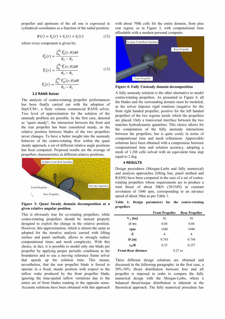
unsteady problem are possible. In the first case, denoted

as “quasi steady”, the interaction between the front and

the rear propeller has been considered steady, as the

relative position between blades of the two propellers

never changes. To have a better insight into the unsteady

behavior of the contra-rotating flow within the quasi

steady approach, a set of different relative angle positions

has been computed. Proposed results are the average of

propellers characteristics at different relative positions.

Figure 3: Quasi Steady domain decomposition at a

given relative angular position.

This is obviously true for co-rotating propellers, while

contra-rotating propellers should be instead properly

designed to exploit the change in the relative position.

However, this approximation, which is almost the same as

adopted for the iterative analysis carried with lifting

surface and panel methods, allows to strongly reduce

computational times and mesh complexity. With this

choice, in fact, it is possible to model only one blade per

propeller by applying proper periodic conditions at the

boundaries and to use a moving reference frame solver

that speeds up the solution time. This means,

nevertheless, that the rear propeller blade is forced to

operate in a fixed, steady position with respect to the

inflow wake produced by the front propeller blade,

ignoring the time/spatial inflow variations due to the

entire set of front blades rotating in the opposite sense.

Accurate solutions have been obtained with this approach

with about 700k cells for the entire domain, front plus

rear region, as in Figure 3, with computational time

affordable with a modern personal computer.

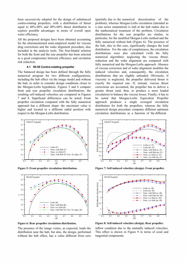
Figure 4: Fully Unsteady domain decomposition

A fully unsteady solution is the other alternative to model

contra-rotating propellers. As presented in Figure 4, all

the blades and the surrounding domain must be modeled,

as the solver imposes rigid rotations (negative for the

front right handed propeller, positive for the left handed

propeller) of the two regions inside which the propellers

are placed. Only a transversal interface between the two

matches hydrodynamic quantities. This choice allows for

the computation of the fully unsteady interactions

between the propellers, but is quite costly in terms of

computational time and mesh refinement. Appreciable

solutions have been obtained with a compromise between

computational time and solution accuracy, adopting a

mesh of 1.2M cells solved with an equivalent time step

equal to 2 deg.

4 RESULTS

Design procedures (Morgan-Lerbs and fully numerical)

and analysis approaches (lifting line, panel method and

RANS) have been compared in the case of a set of contra-

rotating propellers whose requirements are to produce a

total thrust of about 30kN (30154N) at constant

revolution of 1040 rpm, corresponding to an advance

speed of about 36kn as per Table 1.

Table 1: Design parameters for the contra-rotating

propellers

Front Propeller Rear Propeller

VA [kn] 36 36

(1-w) 0.04 0.04

rpm 1040 1040

Z 4 4

D [m] 0.765 0.744

rH/R 0.25 0.257

Front-Rear distance 0.27 m

Three different design solutions are obtained and

discussed in the following paragraphs: in the first case, a

50%-50% thrust distribution between fore and aft

propeller is imposed in order to compare the fully

numerical design with the Morgan-Lerbs, where a

balanced thrust/torque distribution is inherent in the

theoretical approach. The fully numerical procedure has

been successively adopted for the design of unbalanced

contra-rotating propellers, with a distribution of thrust

equal to 60%-40% and 40%-60% thrust distribution to

explore possible advantages in terms of overall open

water efficiency.

All the proposed designs have been obtained accounting

for the aforementioned semi-empirical model for viscous

drag corrections and the wake alignment procedure, also

included in the analysis tools. The four-bladed solution

for both the front and the rear propeller has been selected

as a good compromise between efficiency and cavitation

risk reduction.

4.1 50-50 Contra-rotating propeller

The balanced design has been defined through the fully

numerical program for two different configurations,

including the hub effect via the image model and without

the hub, in order to consider design conditions closer to

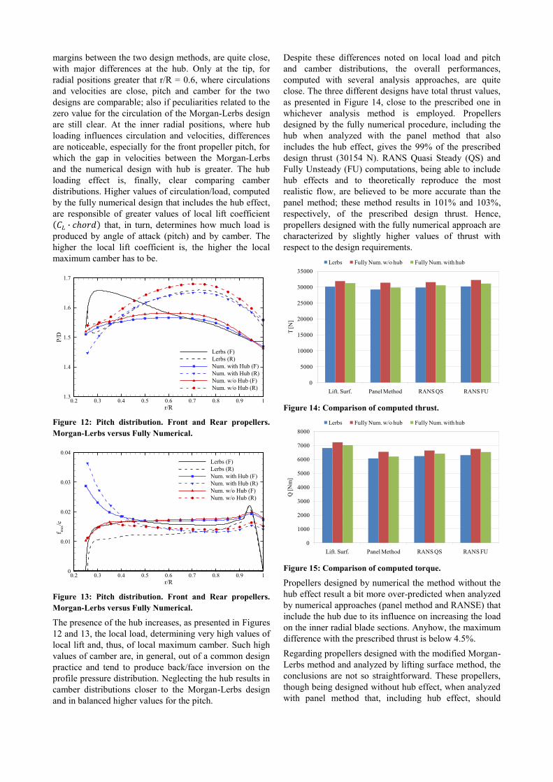
the Morgan-Lerbs hypothesis. Figures 5 and 6 compare

front and rear propeller circulation distributions; the

resulting self-induced velocities are compared in Figures

7 and 8. Significant differences can be noted. Front

propeller circulation computed with the fully numerical

approach has a different shape: the maximum value is

higher and located in a different radial position with

respect to the Morgan-Lerbs distribution.

Figure 5: Front propeller circulation distribution.

Figure 6: Rear propeller circulation distribution.

The presence of the image vortex, as expected, loads the

distribution near the hub, but also, the design, performed

without the hub effect, has a value different from zero

(partially due to the numerical discretization of the

problem), whereas Morgan-Lerbs circulation (intended as

a sine series summation) is null at the hub radius due to

the mathematical treatment of the problem. Circulation

distributions for the rear propeller are similar, in

particular, for the modified Morgan-Lerbs method and the

fully numerical without hub (Figure 6). The presence of

the hub, also in this case, significantly changes the load

distribution. For the sake of completeness, the circulation

distributions were also calculated (with the fully

numerical algorithm); neglecting the viscous thrust,

reduction and the wake alignment are compared with

fully numerical and the Morgan-Lerbs approach. Absence

of viscous correction and of wake alignment modifies the

induced velocities and, consequently, the circulation

distributions that are slightly unloaded. Obviously, if

viscosity is neglected, the propeller delivered thrust is

exactly the required one. If, instead, viscous thrust

corrections are accounted, the propeller has to deliver a

greater thrust (and, thus, to produce a more loaded

circulation) to balance the viscous losses. Finally, it has to

be noted that Morgan-Lerbs Equivalent Propeller

approach produces a single averaged circulation

distribution for both the propellers, whereas the fully

numerical design procedure computes different optimum

circulation distributions as a function of the different

Figure 7: Self-induced velocities (design). Front propeller.

Figure 8: Self-induced velocities (design). Rear propeller.

inflow condition due to the mutually induced velocities.

This effect is shown in Figure 9 in terms of axial and

tangential components.

r/R

0.2 0.3 0.4 0.5 0.6 0.7 0.8 0.9 10

0.1

0.2

0.3

0.4

0.5

0.6

0.7

0.8

Lerbs (F)

Num. with Hub (F)

Num. w/o Hub (F)

Num. with Hub No Visc. No align. (F)

FRONT Propeller

r/R

0.2 0.3 0.4 0.5 0.6 0.7 0.8 0.9 10

0.1

0.2

0.3

0.4

0.5

0.6

0.7

0.8

Lerbs (R)

Num. with Hub (R)

Num. w/o Hub (R)

Num. with Hub No Visc. No align. (R)

REAR Propeller

r/R

Sel

f-in

du

ced

vel

oci

ties

[m/s

]

0.2 0.3 0.4 0.5 0.6 0.7 0.8 0.9 10

0.2

0.4

0.6

0.8

1

1.2

1.4

1.6

1.8

2

Lerbs ax. (F)

Lerbs tan. (F)

Num. with Hub ax. (F)

Num. with Hub tan. (F)

Num. w/o Hub ax. (F)

Num. w/o Hub tan. (F)

FRONT Propeller

r/R

Sel

f-in

du

ced

vel

oci

ties

[m/s

]

0.2 0.3 0.4 0.5 0.6 0.7 0.8 0.9 1-1.5

-1

-0.5

0

0.5

1

1.5

2

Lerbs ax. (R)

Lerbs tan. (R)

Num. with Hub ax. (R)

Num. with Hub tan. (R)

Num. w/o Hub ax. (R)

Num. w/o Hub tan. (R)

REAR Propeller

Figure 9: Induced velocities (by the design codes) on the rear

propeller by the front propeller.

In terms of self-induced velocities, the difference between

the two codes correctly follows the noted difference

between bound circulation distributions. Self-induced

velocities computed by the two codes for the fore

propeller (Figure 7) evidence the major differences

between the design methods, especially with regard to the

tangential component at the inner radial positions. Since

circulation distributions for the rear propeller are very

close, the related self-induced velocities are more similar

(Figure 8) and only the addition of the hub produces a

noticeable influence (Figure 9). A further comparison of

induced velocities is presented in Figures 10 and 11, in

which mean induced velocities on the rear propeller

plane, computed with panel and lifting surface methods,

are compared with induced velocities predicted by the

design codes. Attention is focused on the numerically

designed propellers, including hub and on those obtained

with the modified Morgan-Lerbs method; induced

velocities computed by the analysis codes, namely panel

and lifting surface codes are compared, respectively, with

induced velocities predicted by the fully numerical

approach and by the Morgan-Lerbs procedure. This

comparison is useful in light of the iterative nature of the

design and of the analysis codes that treat each propeller

of the contra-rotating couple as a single propeller

designed or operating in the averaged inflow induced by

the other one. Induced velocities by design procedure and

respective analysis codes are quite close. The hub, when

considered (panel method and fully numerical design

approach), significantly alters the mean distribution of

induced velocity on the rear propeller plane. For the

numerical designed propeller, as in Figure 10, the

presence of the hub during the design phase increases

axial and tangential induced velocities at the inner radial

position. Panel method captures well the presence of the

hub predicting finite value of axial and tangential

velocities, close to those computed with the numerical

design procedure. Some differences are still present and

can be attributed to the exact modeling and to the panel

method of the mathematical singularities (sources) that

represent thickness, which is instead neglected (hub) or

approximated (profile thickness) in the numerical lifting-

line design approach and in the lifting surface analysis

code.

Velocities predicted by the lifting surface code, even if

close to the design values near the tip, have a different

behavior at the hub, especially for what regards the

tangential component.

Figure 10: Induced velocities (by the analysis codes) on the

rear propeller by the front propeller. Propeller designed

with the full numerical method (including hub).

Figure 11: Induced velocities (by the analysis codes) on the

rear propeller by the front propeller. Propeller designed

with the modified Morgan-Lerbs method.

For the designed propeller by modified Morgan-Lerbs

method, predicted velocities by lifting surface are rather

well in agreement with the induced velocities computed

by the design code. Tangential velocities, in particular,

are more similar, due to the fact that both methods,

without modeling the hub, predict a null load at the hub.

The panel method, which allows for the hub effect (and a

finite load there), even in the case of the propeller

designed without considering the hub presence, predicts

higher values of axial and, in particular, tangential

velocities, with an evident different trend when compared

to the lifting surface analysis (Figures 10 and 11).

Differences in bound circulation and induced velocities

play an important role for the definition of propellers

pitch distribution and its maximum position, as presented

in Figure 12 and 13; for front and rear propeller,

respectively. Chord and maximum thickness distributions,

instead, adopting the same cavitation and strength

r/R

Induce

dv

elo

citi

es[m

/s]

0.2 0.3 0.4 0.5 0.6 0.7 0.8 0.9 10

0.5

1

1.5

2

2.5

Lerbs ax.

Lerbs tan.

Num. with Hub ax.

Num. with Hub tan.

Num. w/o Hub ax.

Num. w/o Hub tan.

FRONT on REAR Propeller

r/R

Induce

dv

elo

citi

es[m

/s]

0.2 0.3 0.4 0.5 0.6 0.7 0.8 0.9 10

0.5

1

1.5

2

2.5

3

Design - Num. ax.

Design - Num. tan.

Analysis - Panel ax.

Analysis - Panel tan.

Analysis - Lift. Surf. ax.

Analysis - Lift. Surf. tan.

FRONT on REAR Propeller - Numerical design with hub

r/R

Induce

dv

elo

citi

es[m

/s]

0.2 0.3 0.4 0.5 0.6 0.7 0.8 0.9 10

0.5

1

1.5

2

2.5

3

Design - Lerbs. ax.

Design - Lerbs. tan.

Analysis - Panel ax.

Analysis - Panel tan.

Analysis - Lift. Surf. ax.

Analysis - Lift. Surf. tan.

FRONT on REAR Propeller - Morgan-Lerbs design

margins between the two design methods, are quite close,

with major differences at the hub. Only at the tip, for

radial positions greater that r/R = 0.6, where circulations

and velocities are close, pitch and camber for the two

designs are comparable; also if peculiarities related to the

zero value for the circulation of the Morgan-Lerbs design

are still clear. At the inner radial positions, where hub

loading influences circulation and velocities, differences

are noticeable, especially for the front propeller pitch, for

which the gap in velocities between the Morgan-Lerbs

and the numerical design with hub is greater. The hub

loading effect is, finally, clear comparing camber

distributions. Higher values of circulation/load, computed

by the fully numerical design that includes the hub effect,

are responsible of greater values of local lift coefficient

( ) that, in turn, determines how much load is

produced by angle of attack (pitch) and by camber. The

higher the local lift coefficient is, the higher the local

maximum camber has to be.

Figure 12: Pitch distribution. Front and Rear propellers.

Morgan-Lerbs versus Fully Numerical.

Figure 13: Pitch distribution. Front and Rear propellers.

Morgan-Lerbs versus Fully Numerical.

The presence of the hub increases, as presented in Figures

12 and 13, the local load, determining very high values of

local lift and, thus, of local maximum camber. Such high

values of camber are, in general, out of a common design

practice and tend to produce back/face inversion on the

profile pressure distribution. Neglecting the hub results in

camber distributions closer to the Morgan-Lerbs design

and in balanced higher values for the pitch.

Despite these differences noted on local load and pitch

and camber distributions, the overall performances,

computed with several analysis approaches, are quite

close. The three different designs have total thrust values,

as presented in Figure 14, close to the prescribed one in

whichever analysis method is employed. Propellers

designed by the fully numerical procedure, including the

hub when analyzed with the panel method that also

includes the hub effect, gives the 99% of the prescribed

design thrust (30154 N). RANS Quasi Steady (QS) and

Fully Unsteady (FU) computations, being able to include

hub effects and to theoretically reproduce the most

realistic flow, are believed to be more accurate than the

panel method; these method results in 101% and 103%,

respectively, of the prescribed design thrust. Hence,

propellers designed with the fully numerical approach are

characterized by slightly higher values of thrust with

respect to the design requirements.

Figure 14: Comparison of computed thrust.

Figure 15: Comparison of computed torque.

Propellers designed by numerical the method without the

hub effect result a bit more over-predicted when analyzed

by numerical approaches (panel method and RANSE) that

include the hub due to its influence on increasing the load

on the inner radial blade sections. Anyhow, the maximum

difference with the prescribed thrust is below 4.5%.

Regarding propellers designed with the modified Morgan-

Lerbs method and analyzed by lifting surface method, the

conclusions are not so straightforward. These propellers,

though being designed without hub effect, when analyzed

with panel method that, including hub effect, should

r/R

P/D

0.2 0.3 0.4 0.5 0.6 0.7 0.8 0.9 11.3

1.4

1.5

1.6

1.7

Lerbs (F)

Lerbs (R)

Num. with Hub (F)

Num. with Hub (R)

Num. w/o Hub (F)

Num. w/o Hub (R)

r/R

f max

/c

0.2 0.3 0.4 0.5 0.6 0.7 0.8 0.9 10

0.01

0.02

0.03

0.04

Lerbs (F)

Lerbs (R)

Num. with Hub (F)

Num. with Hub (R)

Num. w/o Hub (F)

Num. w/o Hub (R)

0

5000

10000

15000

20000

25000

30000

35000

Lift. Surf. Panel Method RANS QS RANS FU

T [N

]

Lerbs Fully Num. w/o hub Fully Num. with hub

0

1000

2000

3000

4000

5000

6000

7000

8000

Lift. Surf. Panel Method RANS QS RANS FU

Q [

Nm

]

Lerbs Fully Num. w/o hub Fully Num. with hub

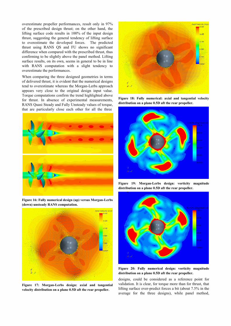
overestimate propeller performances, result only in 97%

of the prescribed design thrust; on the other hand, the

lifting surface code results in 100% of the input design

thrust, suggesting the general tendency of lifting surface

to overestimate the developed forces. The predicted

thrust using RANS QS and FU shows no significant

difference when compared with the prescribed thrust, thus

confirming to be slightly above the panel method. Lifting

surface results, on its own, seems in general to be in line

with RANS computation with a slight tendency to

overestimate the performances.

When comparing the three designed geometries in terms

of delivered thrust, it is evident that the numerical designs

tend to overestimate whereas the Morgan-Lerbs approach

appears very close to the original design input value.

Torque computations confirm the trend highlighted above

for thrust. In absence of experimental measurements,

RANS Quasi Steady and Fully Unsteady values of torque,

that are particularly close each other for all the three

Figure 16: Fully numerical design (up) versus Morgan-Lerbs

(down) unsteady RANS computation.

Figure 17: Morgan-Lerbs design: axial and tangential

velocity distribution on a plane 0.5D aft the rear propeller.

Figure 18: Fully numerical: axial and tangential velocity

distribution on a plane 0.5D aft the rear propeller.

Figure 19: Morgan-Lerbs design: vorticity magnitude

distribution on a plane 0.5D aft the rear propeller.

Figure 20: Fully numerical design: vorticity magnitude

distribution on a plane 0.5D aft the rear propeller.

designs, could be considered as a reference point for

validation. It is clear, for torque more than for thrust, that

lifting surface over-predict forces a bit (about 7.5% in the

average for the three designs), while panel method,

although underestimating results (about 3.5% in the

average), is closer to the reference RANS values.

Moreover, the cavitation free design constraint (required

for both the design approaches) has been confirmed by all

the available analysis tools.

Finally, Figures 16-18 and 19-20 show the velocity

distribution and the vorticity magnitude computed by the

RANS in fully unsteady conditions on a longitudinal

section and on plane 0.5D downstream the rear propeller

for both the designed sets.

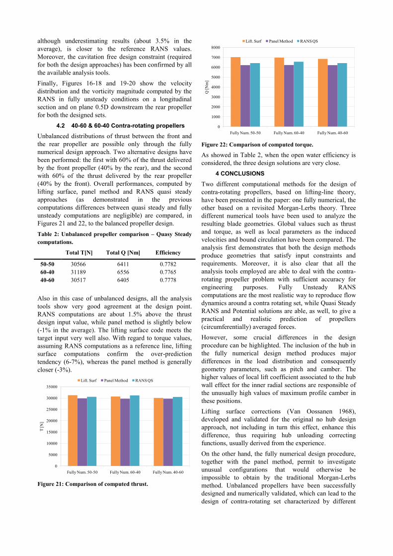
4.2 40-60 & 60-40 Contra-rotating propellers

Unbalanced distributions of thrust between the front and

the rear propeller are possible only through the fully

numerical design approach. Two alternative designs have

been performed: the first with 60% of the thrust delivered

by the front propeller (40% by the rear), and the second

with 60% of the thrust delivered by the rear propeller

(40% by the front). Overall performances, computed by

lifting surface, panel method and RANS quasi steady

approaches (as demonstrated in the previous

computations differences between quasi steady and fully

unsteady computations are negligible) are compared, in

Figures 21 and 22, to the balanced propeller design.

Table 2: Unbalanced propeller comparison – Quasy Steady

computations.

Total T[N] Total Q [Nm] Efficiency

50-50 30566 6411 0.7782

60-40 31189 6556 0.7765

40-60 30517 6405 0.7778

Also in this case of unbalanced designs, all the analysis

tools show very good agreement at the design point.

RANS computations are about 1.5% above the thrust

design input value, while panel method is slightly below

(-1% in the average). The lifting surface code meets the

target input very well also. With regard to torque values,

assuming RANS computations as a reference line, lifting

surface computations confirm the over-prediction

tendency (6-7%), whereas the panel method is generally

closer (-3%).

Figure 21: Comparison of computed thrust.

Figure 22: Comparison of computed torque.

As showed in Table 2, when the open water efficiency is

considered, the three design solutions are very close.

4 CONCLUSIONS

Two different computational methods for the design of

contra-rotating propellers, based on lifting-line theory,

have been presented in the paper: one fully numerical, the

other based on a revisited Morgan-Lerbs theory. Three

different numerical tools have been used to analyze the

resulting blade geometries. Global values such as thrust

and torque, as well as local parameters as the induced

velocities and bound circulation have been compared. The

analysis first demonstrates that both the design methods

produce geometries that satisfy input constraints and

requirements. Moreover, it is also clear that all the

analysis tools employed are able to deal with the contra-

rotating propeller problem with sufficient accuracy for

engineering purposes. Fully Unsteady RANS

computations are the most realistic way to reproduce flow

dynamics around a contra rotating set, while Quasi Steady

RANS and Potential solutions are able, as well, to give a

practical and realistic prediction of propellers

(circumferentially) averaged forces.

However, some crucial differences in the design

procedure can be highlighted. The inclusion of the hub in

the fully numerical design method produces major

differences in the load distribution and consequently

geometry parameters, such as pitch and camber. The

higher values of local lift coefficient associated to the hub

wall effect for the inner radial sections are responsible of

the unusually high values of maximum profile camber in

these positions.

Lifting surface corrections (Van Oossanen 1968),

developed and validated for the original no hub design

approach, not including in turn this effect, enhance this

difference, thus requiring hub unloading correcting

functions, usually derived from the experience.

On the other hand, the fully numerical design procedure,

together with the panel method, permit to investigate

unusual configurations that would otherwise be

impossible to obtain by the traditional Morgan-Lerbs

method. Unbalanced propellers have been successfully

designed and numerically validated, which can lead to the

design of contra-rotating set characterized by different

0

5000

10000

15000

20000

25000

30000

35000

Fully Num. 50-50 Fully Num. 60-40 Fully Num. 40-60

T [N

]

Lift. Surf Panel Method RANS QS

0

1000

2000

3000

4000

5000

6000

7000

8000

Fully Num. 50-50 Fully Num. 60-40 Fully Num. 40-60

Q [

Nm

]

Lift. Surf Panel Method RANS QS

number of blades and different rate of revolutions

between the front and the rear propeller. The possibility to

have different number of blades between the fore and the

aft propeller could help in avoiding the potential risk of

resonance subsequent to the choice of an equal number of

blades.

REFERENCES

Brizzolara, S., Grassi, D. & Tincani, E. (2008). „Design of

Contra-Rotating Propellers for High Speed Stern

Thrusters‟. Ship and Offshore Structures 2(1), pp.169-

182.

Castagneto, E. & Maioli, P. G. (1968). „Theoretical and

experimental study on the dynamics of hydrofoils as

applied to naval propellers‟. Proceedings of the 7th

Symposium on Naval Hydrodynamics, Rome, Italy.

Coney, W. B. (1989). A Method for the Design of a class

of Optimum Marine Propellers. PhD Thesis,

Massachusetts Institute of Technology.

Connolly, J. E. (1961). „Strength of Propellers‟.

Transaction of the Royal Institution of Naval

Architects 103, pp. 139-154.

Gaggero, S. & Brizzolara, S. (2009). „A Panel Method for

Trans-Cavitating Marine Propellers‟. Proceedings of

the 7th International Symposium on Cavitation, Ann

Arbor, Michigan, United States.

Grassi, D. & Brizzolara, S. (2007), „Numerical Analysis

of Propeller Performance by Lifting Surface Theory‟.

Proceeding of the 2nd Int. Conf. on Marine Research

and Transportation, Ischia, Naples, Italy.

Grossi, L. (1980). „PESP: un programma integrato per la

progettazione di eliche navali con la teoria della

superficie portante‟. CETENA Report 1022, (in

Italian).

Kerwin, J. E. & Lee, C. S. (1978) „Prediction of Steady

and Unsteady Marine Propeller Performance by

Numerical Lifting Surface Theory‟. Trans. Society of

Naval Architects and Marine Engineers 86, pp. 218-

253.

Lerbs, H. W. (1952). „Moderately loaded propellers with

a finite number of blades and an arbitrary distribution

of circulation‟. Transaction of the Society of Naval

Architects and Marine Engineers 60, pp. 6-31.

Morgan, W. B. (1960). „The design of counter-rotating

propellers using Lerbs‟. Transaction of the Society of

Naval Architects and Marine Engineers 68, pp. 6-31.

Van Oossanen, P. (1968). „Calculation of Performance

and Cavitation Characteristics of Propellers Including

Effects of Non Uniform Flow and Viscosity‟.

Netherland Ship Model Basin Report 457.