Embed Size (px)
Citation preview
From Relational Statistics to Degrees of Belief
School of Computing Science Simon Fraser University Vancouver, Canada
Tianxiang Gao
Yuke Zhu
2
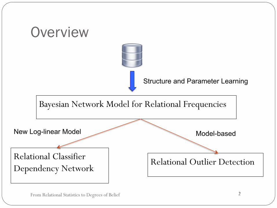
Overview
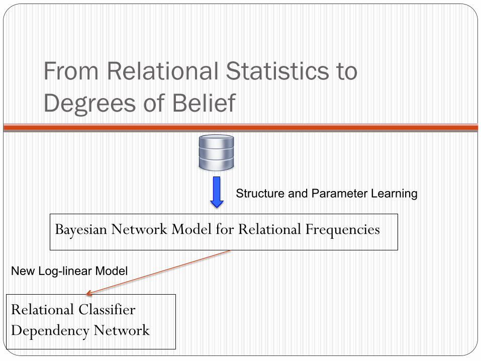
From Relational Statistics to Degrees of Belief
Bayesian Network Model for Relational Frequencies
Relational Classifier Dependency Network
Relational Outlier Detection
Structure and Parameter Learning
New Log-linear Model Model-based
Relational Data and Logic
From Relational Statistics to Degrees of Belief
Lise Getoor David Poole Stuart Russsell
4
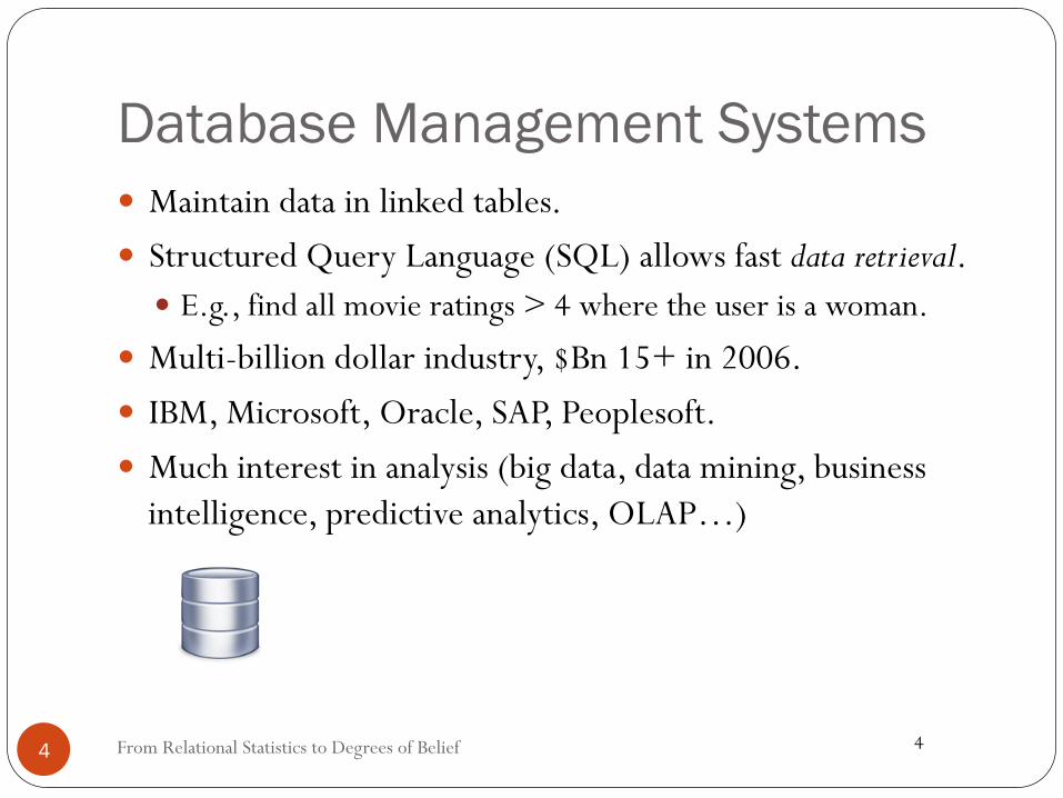
Database Management Systems
From Relational Statistics to Degrees of Belief 4
� Maintain data in linked tables. � Structured Query Language (SQL) allows fast data retrieval.
� E.g., find all movie ratings > 4 where the user is a woman.
� Multi-billion dollar industry, $Bn 15+ in 2006. � IBM, Microsoft, Oracle, SAP, Peoplesoft. � Much interest in analysis (big data, data mining, business
intelligence, predictive analytics, OLAP…)
5
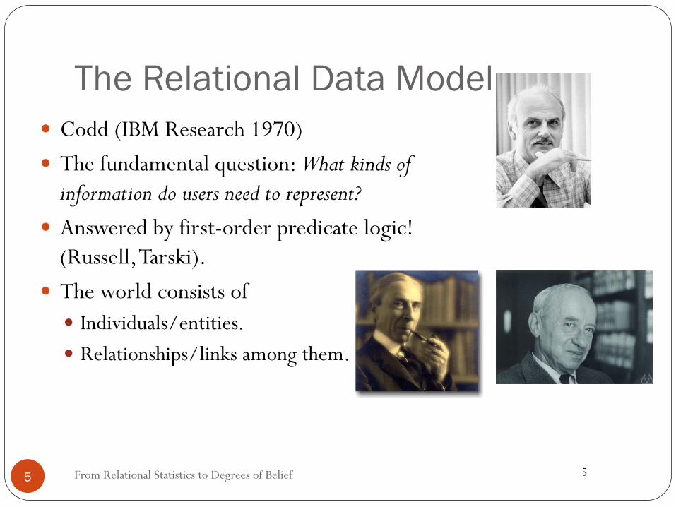
The Relational Data Model
From Relational Statistics to Degrees of Belief 5
� Codd (IBM Research 1970) � The fundamental question: What kinds of
information do users need to represent? � Answered by first-order predicate logic!
(Russell, Tarski). � The world consists of
� Individuals/entities. � Relationships/links among them.
6
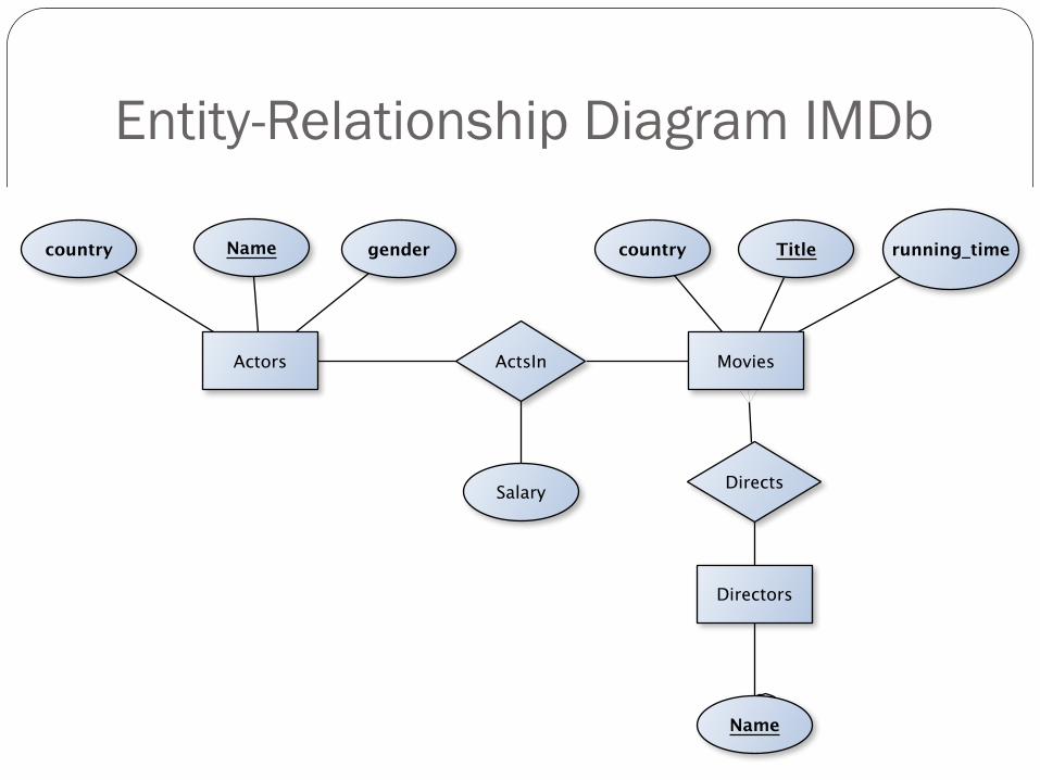
Entity-Relationship Diagram IMDb
From Relational Statistics to Degrees of Belief 6
7 From Relational Statistics to Degrees of Belief 7
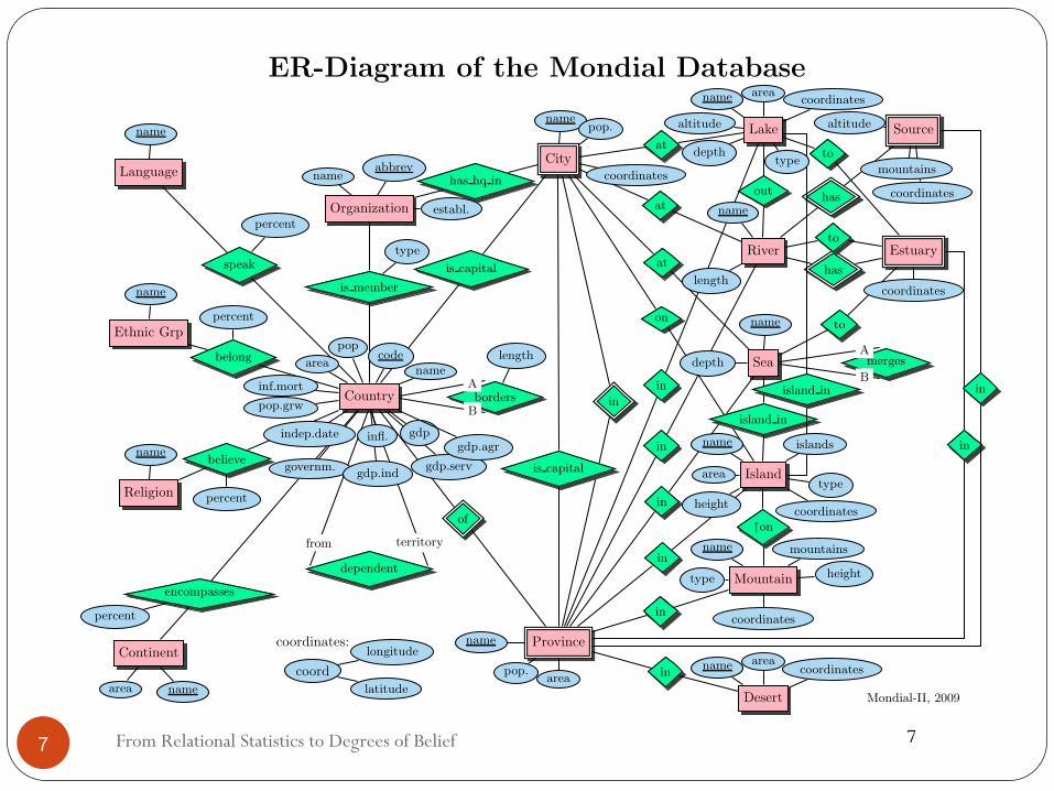
ER-Diagram of the Mondial Database
Language
Ethnic Grp
Religion
Continent
City
Organization
Country
coordinates: Province
coord
Lake Source
River Estuary
Sea
Island
Mountain
Desert Mondial-II, 2009
longitude
latitude
is capital
in
is capital
of
is member
has hq in
encompasses
bordersA
B
dependent
territoryfrom
in
in
in
in
in
in
at
at
at
on
↑on
outhas
has
to
to
to
in
in
island in
island in
mergesA
B
belong
believe
speak
namepop.
coordinatesabbrev
name
establ.
type
lengthname
codepop
area
inf.mort
pop.grw
governm.
indep.date
gdp.ind
infl.
gdp.serv
gdpgdp.agr
namearea
name
percent
name
percent
name
percent
percent
name
pop.area
name areacoordinates
altitude
depthtype
name
length
altitude
coordinates
mountains
coordinates
name
depth
name mountains
heighttype
coordinates
name islands
area
height
type
coordinates
name areacoordinates
8
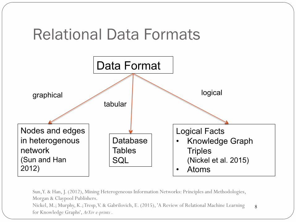
Relational Data Formats
Sun, Y. & Han, J. (2012), Mining Heterogeneous Information Networks: Principles and Methodologies, Morgan & Claypool Publishers. Nickel, M.; Murphy, K.; Tresp, V. & Gabrilovich, E. (2015), 'A Review of Relational Machine Learning for Knowledge Graphs', ArXiv e-prints .
graphical
Data Format
Nodes and edges in heterogenous network (Sun and Han 2012)
Database Tables SQL
Logical Facts • Knowledge Graph
Triples (Nickel et al. 2015)
• Atoms
tabular logical
9
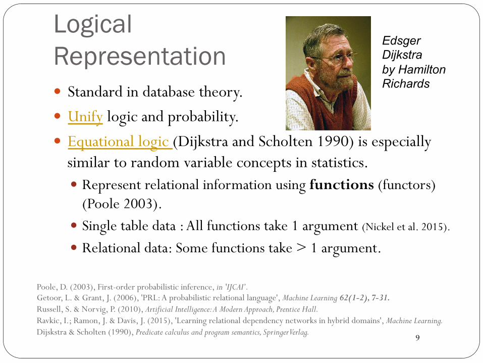
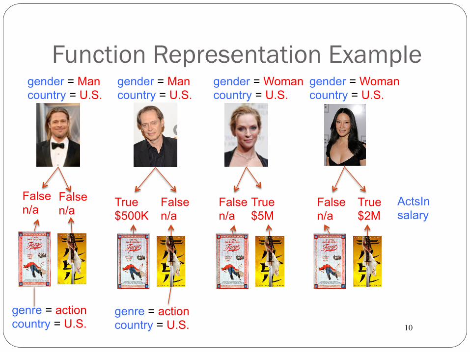
Logical Representation � Standard in database theory. � Unify logic and probability. � Equational logic (Dijkstra and Scholten 1990) is especially
similar to random variable concepts in statistics. � Represent relational information using functions (functors)
(Poole 2003). � Single table data : All functions take 1 argument (Nickel et al. 2015).
� Relational data: Some functions take > 1 argument.
Poole, D. (2003), First-order probabilistic inference, in 'IJCAI’. Getoor, L. & Grant, J. (2006), 'PRL: A probabilistic relational language', Machine Learning 62(1-2), 7-31. Russell, S. & Norvig, P. (2010), Artificial Intelligence: A Modern Approach, Prentice Hall. Ravkic, I.; Ramon, J. & Davis, J. (2015), 'Learning relational dependency networks in hybrid domains', Machine Learning. Dijskstra & Scholten (1990), Predicate calculus and program semantics, Springer Verlag.
Edsger Dijkstra by Hamilton Richards
10
Function Representation Example
True $500K
True $5M
True $2M
False n/a
ActsIn salary
False n/a
False n/a
False n/a
False n/a
gender = Man country = U.S.
gender = Man country = U.S.
gender = Woman country = U.S.
gender = Woman country = U.S.
genre = action country = U.S.
genre = action country = U.S.
11
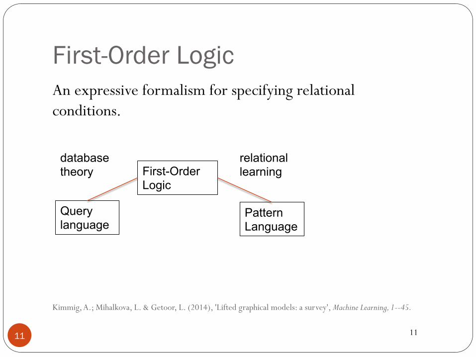
First-Order Logic
Kimmig, A.; Mihalkova, L. & Getoor, L. (2014), 'Lifted graphical models: a survey', Machine Learning, 1--45.
11
An expressive formalism for specifying relational conditions.
First-Order Logic
Query language
Pattern Language
database theory
relational learning
12
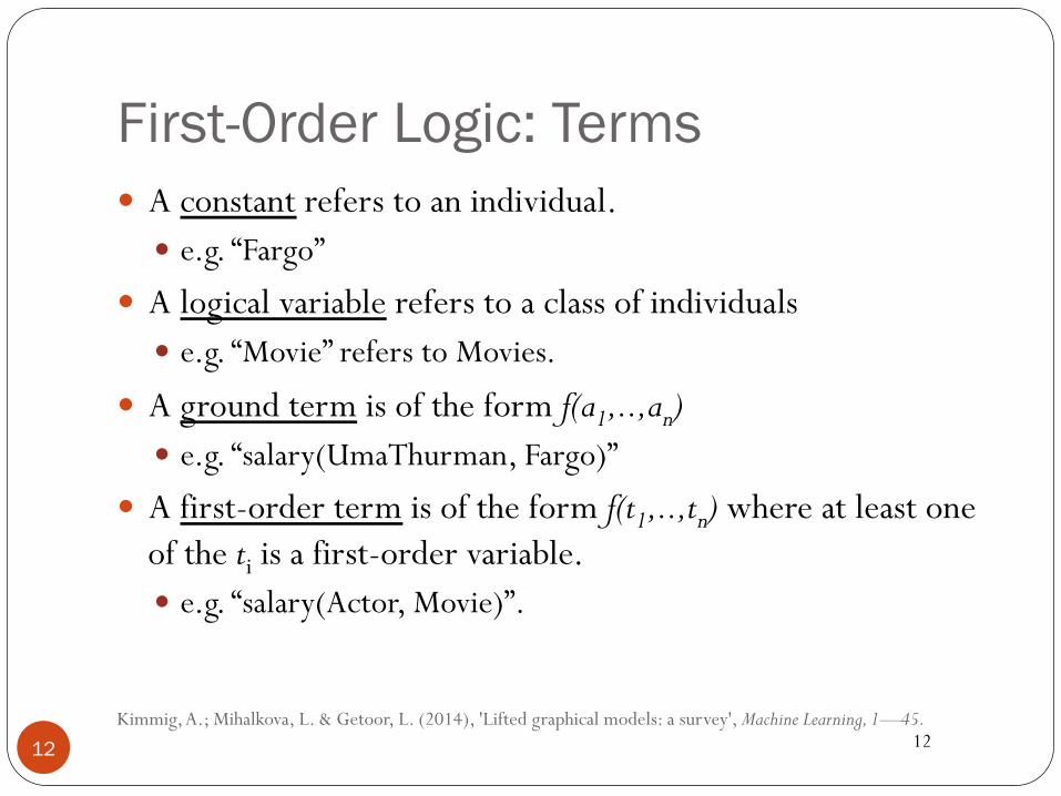
First-Order Logic: Terms
Kimmig, A.; Mihalkova, L. & Getoor, L. (2014), 'Lifted graphical models: a survey', Machine Learning, 1—45.
12
� A constant refers to an individual. � e.g. “Fargo”
� A logical variable refers to a class of individuals � e.g. “Movie” refers to Movies.
� A ground term is of the form f(a1,..,an) � e.g. “salary(UmaThurman, Fargo)”
� A first-order term is of the form f(t1,..,tn) where at least one of the ti is a first-order variable. � e.g. “salary(Actor, Movie)”.
13
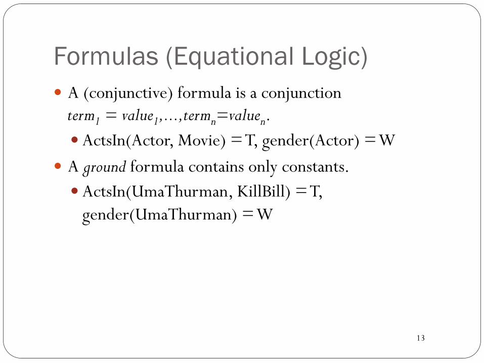
Formulas (Equational Logic) � A (conjunctive) formula is a conjunction
term1 = value1,...,termn=valuen. � ActsIn(Actor, Movie) = T, gender(Actor) = W
� A ground formula contains only constants. � ActsIn(UmaThurman, KillBill) = T,
gender(UmaThurman) = W
Two Kinds of Probability
Frequencies vs. Single Event Probabilities
From Relational Statistics to Degrees of Belief
Joe Halpern Fahim Bacchus
15
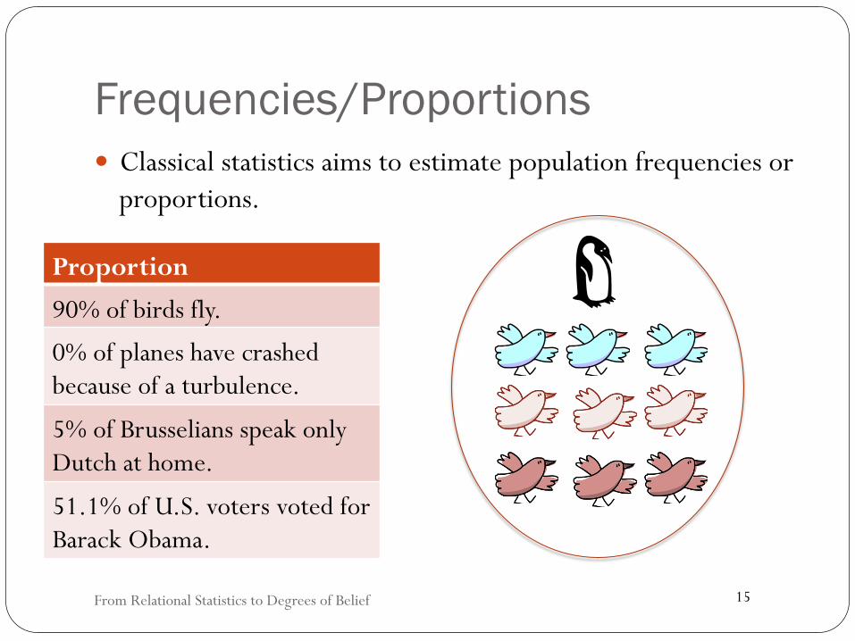
Frequencies/Proportions � Classical statistics aims to estimate population frequencies or
proportions.
From Relational Statistics to Degrees of Belief
Proportion 90% of birds fly.
0% of planes have crashed because of a turbulence.
5% of Brusselians speak only Dutch at home.
51.1% of U.S. voters voted for Barack Obama.
16
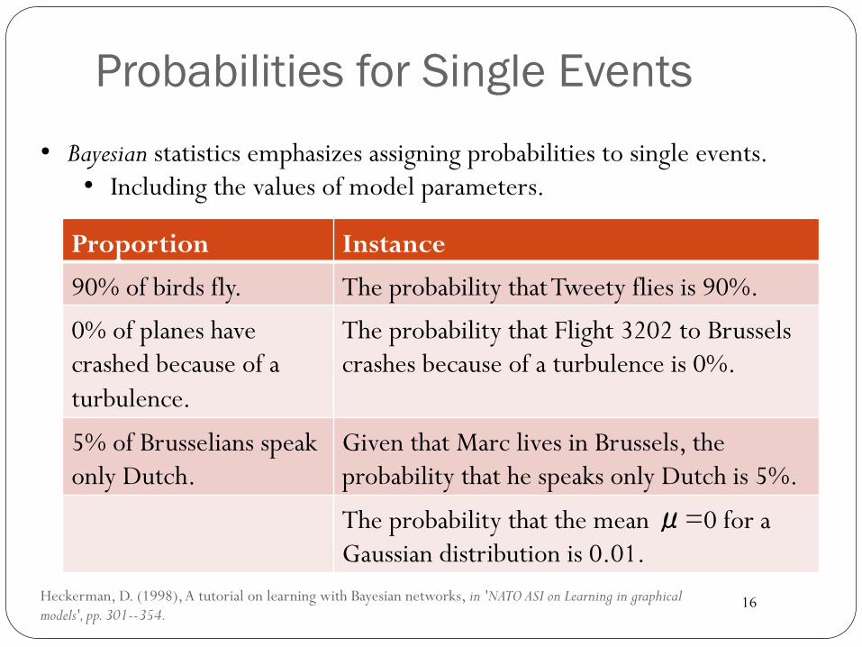
Probabilities for Single Events
Proportion Instance 90% of birds fly. The probability that Tweety flies is 90%.
0% of planes have crashed because of a turbulence.
The probability that Flight 3202 to Brussels crashes because of a turbulence is 0%.
5% of Brusselians speak only Dutch.
Given that Marc lives in Brussels, the probability that he speaks only Dutch is 5%.
The probability that the mean μ=0 for a Gaussian distribution is 0.01.
Heckerman, D. (1998), A tutorial on learning with Bayesian networks, in 'NATO ASI on Learning in graphical models', pp. 301--354.
• Bayesian statistics emphasizes assigning probabilities to single events. • Including the values of model parameters.
17
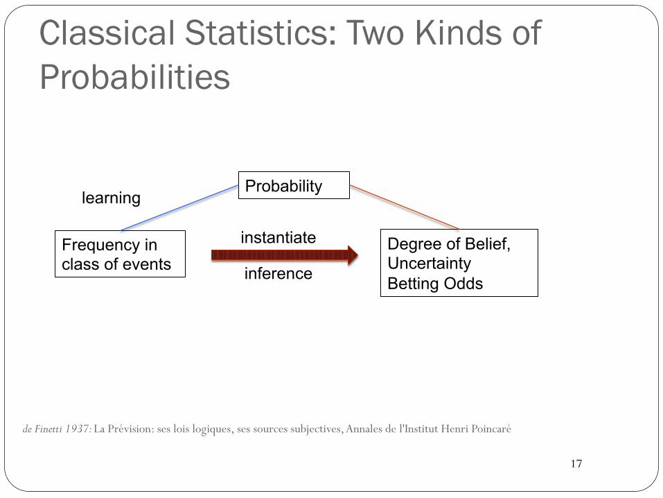
Classical Statistics: Two Kinds of Probabilities
de Finetti 1937: La Prévision: ses lois logiques, ses sources subjectives, Annales de l'Institut Henri Poincaré
Probability
Frequency in class of events
Degree of Belief, Uncertainty Betting Odds
learning
instantiate
inference
18
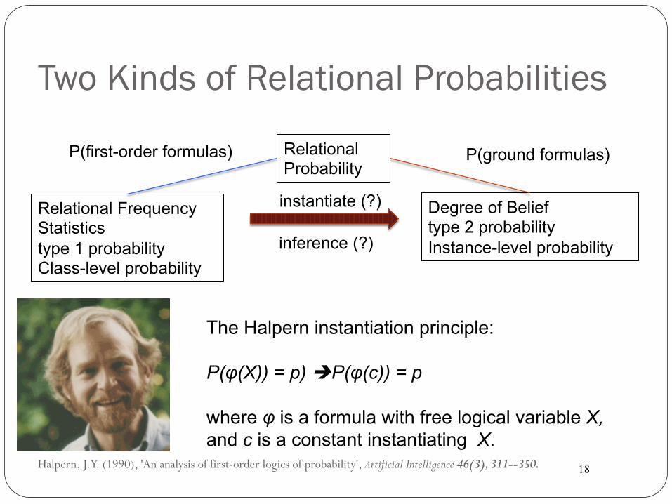
Two Kinds of Relational Probabilities
Halpern, J. Y. (1990), 'An analysis of first-order logics of probability', Artificial Intelligence 46(3), 311--350.
Relational Probability
Relational Frequency Statistics type 1 probability Class-level probability
Degree of Belief type 2 probability Instance-level probability
P(first-order formulas) P(ground formulas)
instantiate (?)
The Halpern instantiation principle: P(φ(X)) = p) !P(φ(c)) = p where φ is a formula with free logical variable X, and c is a constant instantiating X.
inference (?)
19
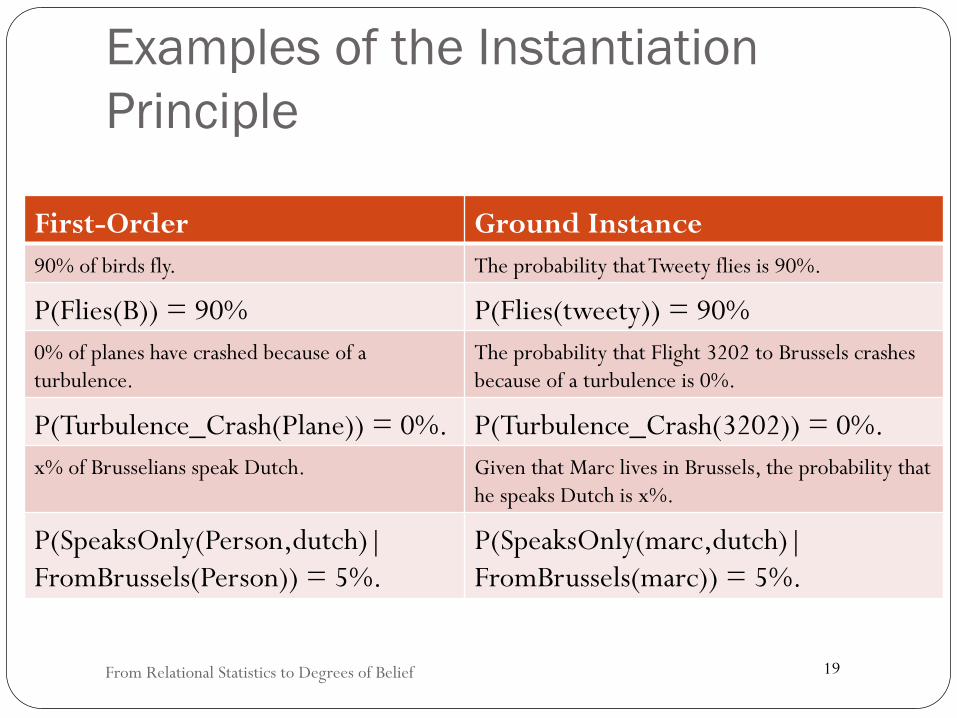
Examples of the Instantiation Principle
From Relational Statistics to Degrees of Belief
First-Order Ground Instance 90% of birds fly. The probability that Tweety flies is 90%.
P(Flies(B)) = 90% P(Flies(tweety)) = 90% 0% of planes have crashed because of a turbulence.
The probability that Flight 3202 to Brussels crashes because of a turbulence is 0%.
P(Turbulence_Crash(Plane)) = 0%. P(Turbulence_Crash(3202)) = 0%. x% of Brusselians speak Dutch. Given that Marc lives in Brussels, the probability that
he speaks Dutch is x%.
P(SpeaksOnly(Person,dutch)|FromBrussels(Person)) = 5%.
P(SpeaksOnly(marc,dutch)|FromBrussels(marc)) = 5%.
20
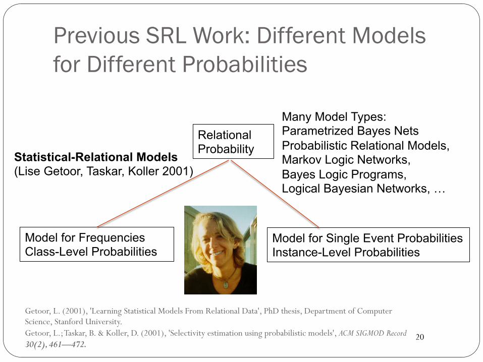
Previous SRL Work: Different Models for Different Probabilities
Getoor, L. (2001), 'Learning Statistical Models From Relational Data', PhD thesis, Department of Computer Science, Stanford University. Getoor, L.; Taskar, B. & Koller, D. (2001), 'Selectivity estimation using probabilistic models', ACM SIGMOD Record 30(2), 461—472.
Model for Frequencies Class-Level Probabilities
Model for Single Event Probabilities Instance-Level Probabilities
Statistical-Relational Models (Lise Getoor, Taskar, Koller 2001)
Many Model Types: Parametrized Bayes Nets Probabilistic Relational Models, Markov Logic Networks, Bayes Logic Programs, Logical Bayesian Networks, …
Relational Probability
21
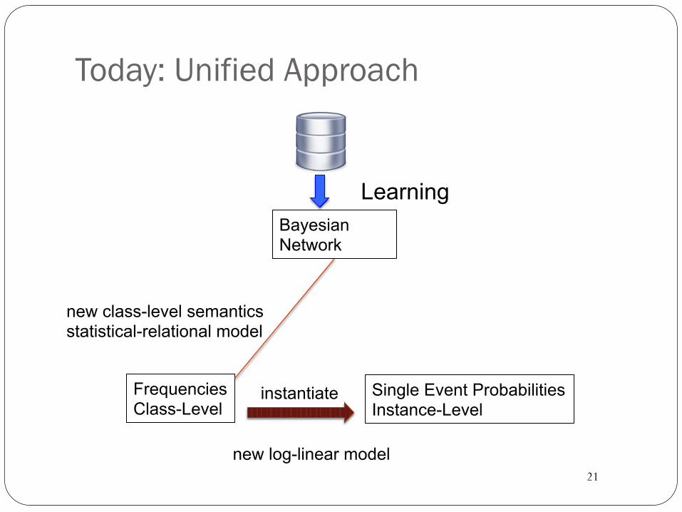
Today: Unified Approach
Frequencies Class-Level
Single Event Probabilities Instance-Level
new class-level semantics statistical-relational model
Bayesian Network
instantiate
Learning
new log-linear model

Relational Frequencies
From Relational Statistics to Degrees of Belief
Joe Halpern Fahim Bacchus
23
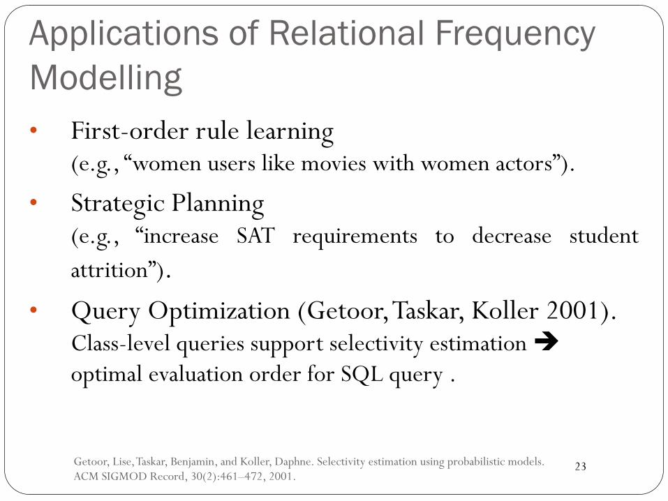
Applications of Relational Frequency Modelling • First-order rule learning
(e.g., “women users like movies with women actors”).
• Strategic Planning (e.g., “increase SAT requirements to decrease student attrition”).
• Query Optimization (Getoor, Taskar, Koller 2001). Class-level queries support selectivity estimation è optimal evaluation order for SQL query .
Getoor, Lise, Taskar, Benjamin, and Koller, Daphne. Selectivity estimation using probabilistic models. ACM SIGMOD Record, 30(2):461–472, 2001.
24
Relational Frequencies
From Relational Statistics to Degrees of Belief
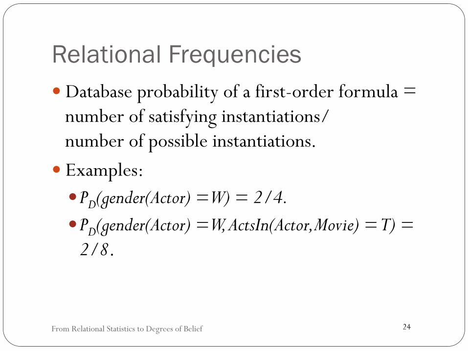
� Database probability of a first-order formula = number of satisfying instantiations/ number of possible instantiations.
� Examples: � PD(gender(Actor) = W) = 2/4. � PD(gender(Actor) = W, ActsIn(Actor,Movie) = T) =
2/8.
25
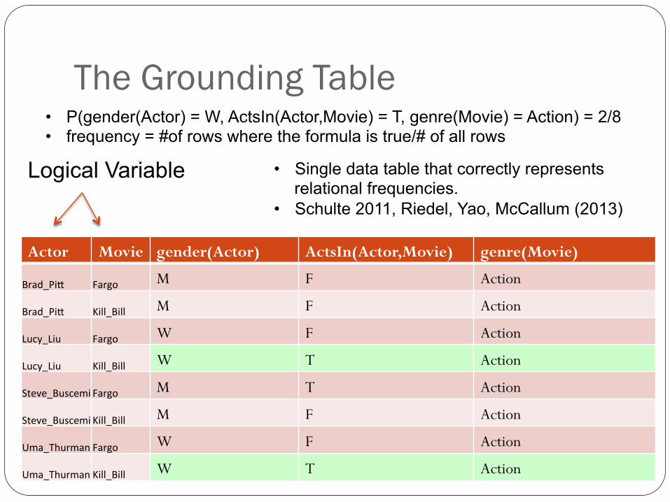
The Grounding Table
Actor Movie gender(Actor) ActsIn(Actor,Movie) genre(Movie)
Brad_Pi( Fargo M F Action
Brad_Pi( Kill_Bill M F Action
Lucy_Liu Fargo W F Action
Lucy_Liu Kill_Bill W T Action
Steve_BuscemiFargo M T Action
Steve_BuscemiKill_Bill M F Action
Uma_ThurmanFargo W F Action
Uma_ThurmanKill_Bill W T Action
• P(gender(Actor) = W, ActsIn(Actor,Movie) = T, genre(Movie) = Action) = 2/8 • frequency = #of rows where the formula is true/# of all rows
Logical Variable • Single data table that correctly represents relational frequencies.
• Schulte 2011, Riedel, Yao, McCallum (2013)
26
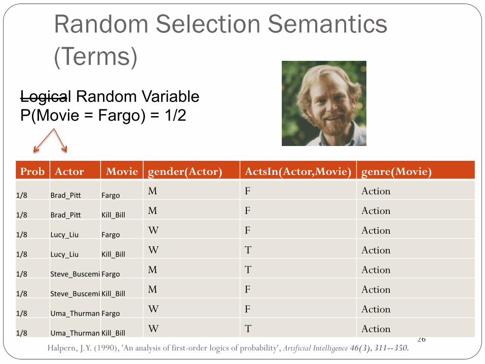
Random Selection Semantics (Terms)
Prob Actor Movie gender(Actor) ActsIn(Actor,Movie) genre(Movie)
1/8 Brad_Pi( Fargo M F Action
1/8 Brad_Pi( Kill_Bill M F Action
1/8 Lucy_Liu Fargo W F Action
1/8 Lucy_Liu Kill_Bill W T Action
1/8 Steve_BuscemiFargo M T Action
1/8 Steve_BuscemiKill_Bill M F Action
1/8 Uma_ThurmanFargo W F Action
1/8 Uma_ThurmanKill_Bill W T Action
Halpern, J. Y. (1990), 'An analysis of first-order logics of probability', Artificial Intelligence 46(3), 311--350.
Logical Random Variable P(Movie = Fargo) = 1/2
27
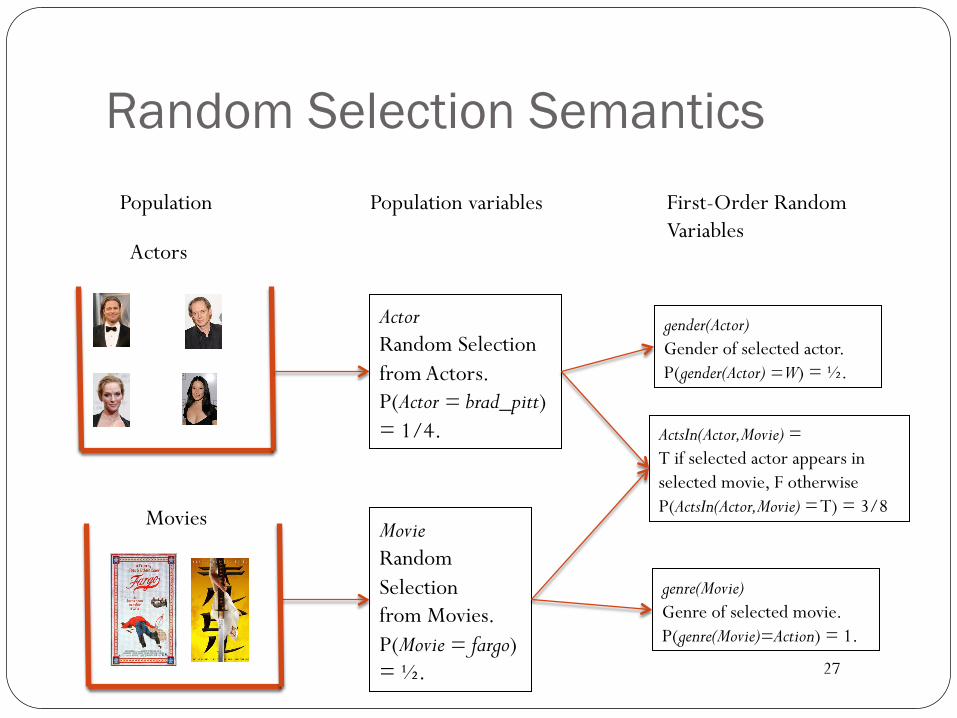
Population
Actors
Population variables
Actor Random Selection from Actors. P(Actor = brad_pitt) = 1/4.
Movie Random Selection from Movies. P(Movie = fargo) = ½.
First-Order Random Variables
gender(Actor) Gender of selected actor. P(gender(Actor) = W) = ½.
genre(Movie) Genre of selected movie. P(genre(Movie)=Action) = 1.
ActsIn(Actor,Movie) = T if selected actor appears in selected movie, F otherwise P(ActsIn(Actor,Movie) = T) = 3/8
Random Selection Semantics
Movies
Bayesian Networks for Relational Statistics Statistical-Relational Models (SRMs) Random Selection Semantics for Bayesian Networks
From Relational Statistics to Degrees of Belief
Bayesian Network Model for Relational Frequencies
29
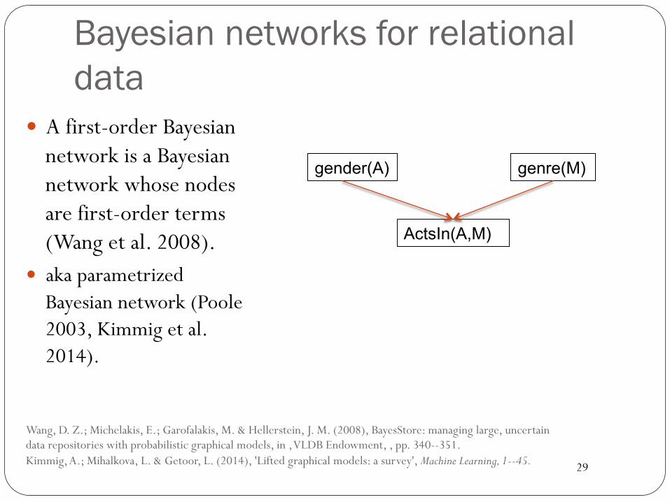
Bayesian networks for relational data
� A first-order Bayesian network is a Bayesian network whose nodes are first-order terms (Wang et al. 2008).
� aka parametrized Bayesian network (Poole 2003, Kimmig et al. 2014).
Wang, D. Z.; Michelakis, E.; Garofalakis, M. & Hellerstein, J. M. (2008), BayesStore: managing large, uncertain data repositories with probabilistic graphical models, in , VLDB Endowment, , pp. 340--351. Kimmig, A.; Mihalkova, L. & Getoor, L. (2014), 'Lifted graphical models: a survey', Machine Learning, 1--45.
gender(A)
ActsIn(A,M)
genre(M)
30
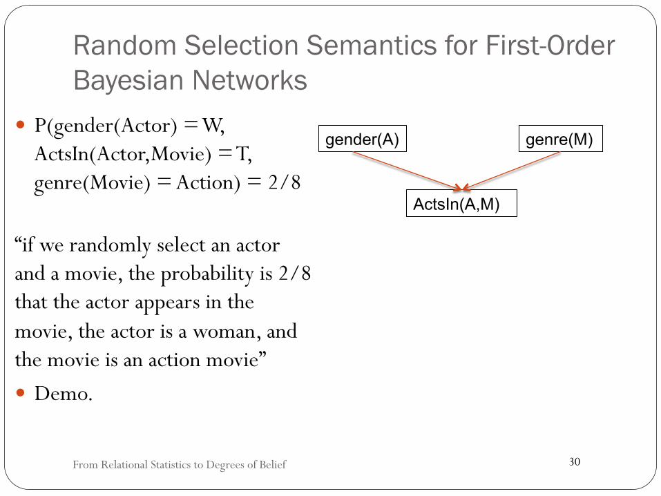
Random Selection Semantics for First-Order Bayesian Networks
� P(gender(Actor) = W, ActsIn(Actor,Movie) = T, genre(Movie) = Action) = 2/8
“if we randomly select an actor and a movie, the probability is 2/8 that the actor appears in the movie, the actor is a woman, and the movie is an action movie” � Demo.
From Relational Statistics to Degrees of Belief
gender(A)
ActsIn(A,M)
genre(M)
31
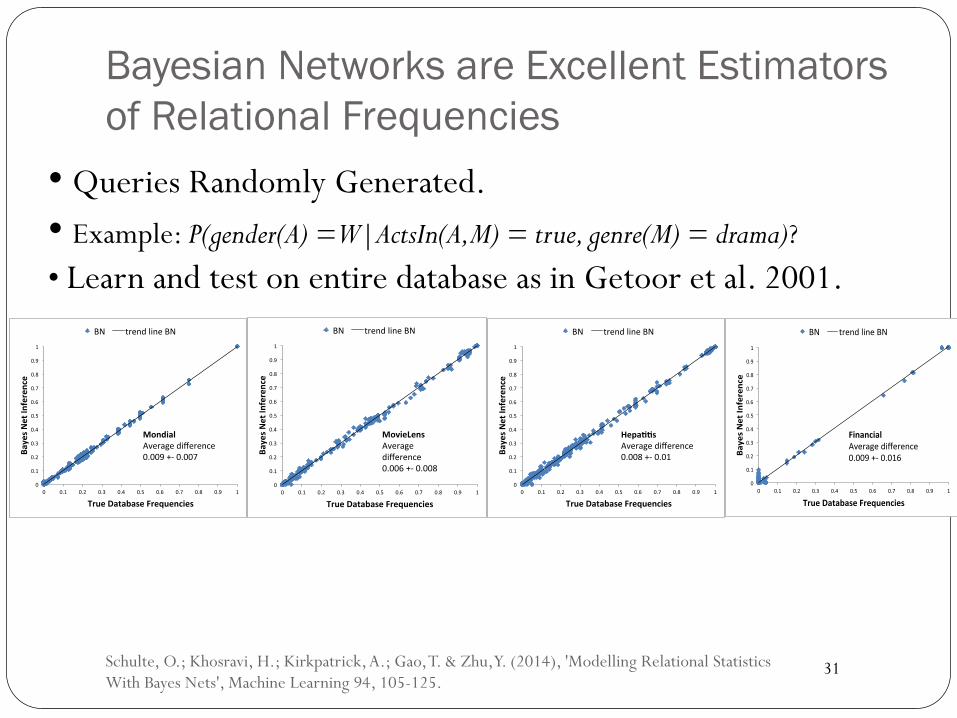
Bayesian Networks are Excellent Estimators of Relational Frequencies
• Queries Randomly Generated. • Example: P(gender(A) = W|ActsIn(A,M) = true, genre(M) = drama)? • Learn and test on entire database as in Getoor et al. 2001.
0"
0.1"
0.2"
0.3"
0.4"
0.5"
0.6"
0.7"
0.8"
0.9"
1"
0" 0.1" 0.2" 0.3" 0.4" 0.5" 0.6" 0.7" 0.8" 0.9" 1"
Bayes&N
et&In
ference&
True&Database&Frequencies&
BN" trend"line"BN"
Hepa77s&Average"difference""0.008"+="0.01"
0"
0.1"
0.2"
0.3"
0.4"
0.5"
0.6"
0.7"
0.8"
0.9"
1"
0" 0.1" 0.2" 0.3" 0.4" 0.5" 0.6" 0.7" 0.8" 0.9" 1"
Bayes&N
et&In
ference&
True&Database&Frequencies&
BN" trend"line"BN"
MovieLens&Average"difference""0.006"+="0.008"
0"
0.1"
0.2"
0.3"
0.4"
0.5"
0.6"
0.7"
0.8"
0.9"
1"
0" 0.1" 0.2" 0.3" 0.4" 0.5" 0.6" 0.7" 0.8" 0.9" 1"
Bayes&N
et&In
ference&
True&Database&Frequencies&
BN" trend"line"BN"
Mondial&Average"difference""0.009"+="0.007"
0"
0.1"
0.2"
0.3"
0.4"
0.5"
0.6"
0.7"
0.8"
0.9"
1"
0" 0.1" 0.2" 0.3" 0.4" 0.5" 0.6" 0.7" 0.8" 0.9" 1"
Bayes&Net&In
ference&
True&Database&Frequencies&
BN" trend"line"BN"
Financial&Average"difference"0.009"+="0.016"
Schulte, O.; Khosravi, H.; Kirkpatrick, A.; Gao, T. & Zhu, Y. (2014), 'Modelling Relational Statistics With Bayes Nets', Machine Learning 94, 105-125.
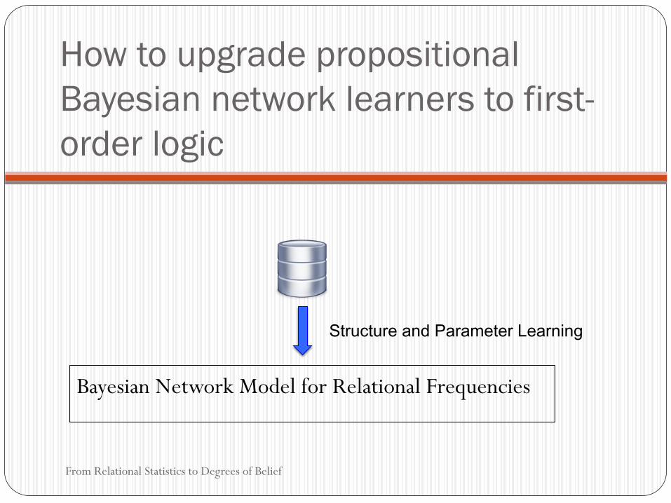
How to upgrade propositional Bayesian network learners to first-order logic
From Relational Statistics to Degrees of Belief
Bayesian Network Model for Relational Frequencies
Structure and Parameter Learning
33
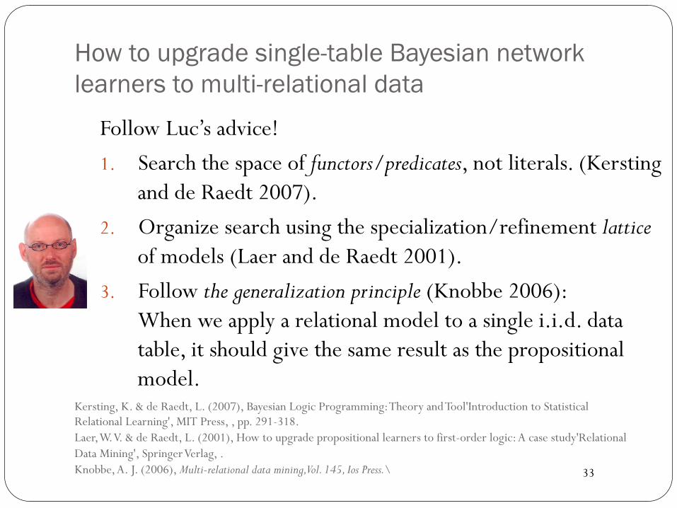
How to upgrade single-table Bayesian network learners to multi-relational data
Follow Luc’s advice! 1. Search the space of functors/predicates, not literals. (Kersting
and de Raedt 2007). 2. Organize search using the specialization/refinement lattice
of models (Laer and de Raedt 2001). 3. Follow the generalization principle (Knobbe 2006):
When we apply a relational model to a single i.i.d. data table, it should give the same result as the propositional model.
Kersting, K. & de Raedt, L. (2007), Bayesian Logic Programming: Theory and Tool'Introduction to Statistical Relational Learning', MIT Press, , pp. 291-318. Laer, W. V. & de Raedt, L. (2001), How to upgrade propositional learners to first-order logic: A case study'Relational Data Mining', Springer Verlag, . Knobbe, A. J. (2006), Multi-relational data mining, Vol. 145, Ios Press.\
34
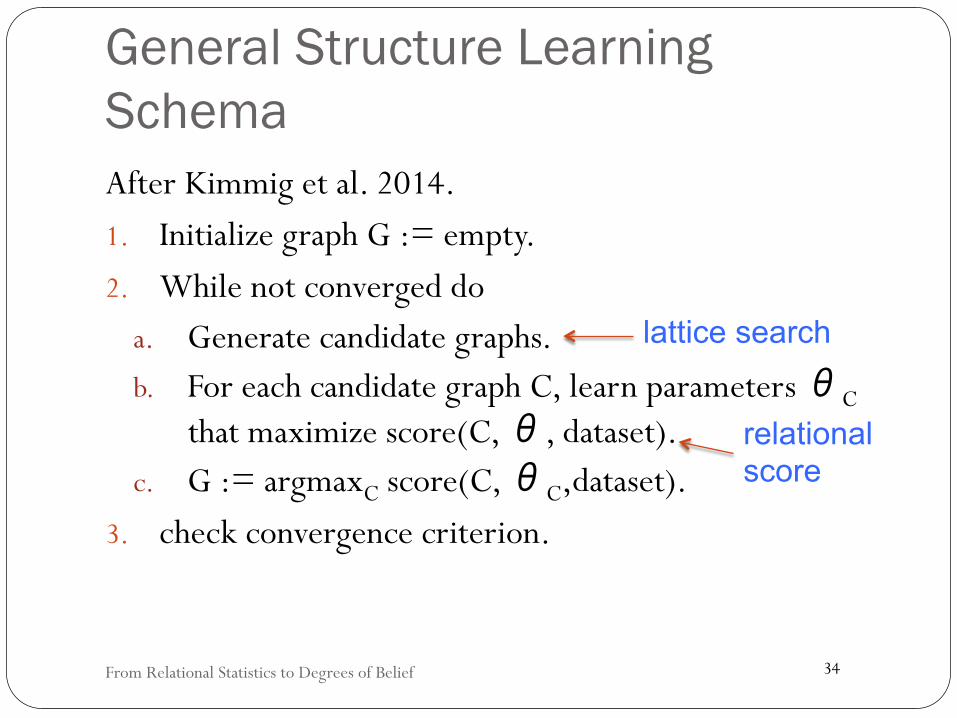
General Structure Learning Schema After Kimmig et al. 2014. 1. Initialize graph G := empty. 2. While not converged do
a. Generate candidate graphs. b. For each candidate graph C, learn parameters θC
that maximize score(C, θ, dataset). c. G := argmaxC score(C, θC,dataset).
3. check convergence criterion.
From Relational Statistics to Degrees of Belief
lattice search
relational score
Scoring Bayesian Networks for Relational Data
From Relational Statistics to Degrees of Belief
36
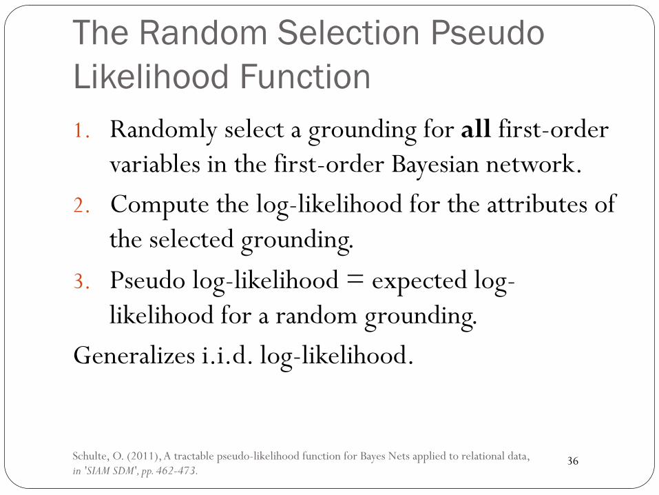
The Random Selection Pseudo Likelihood Function 1. Randomly select a grounding for all first-order
variables in the first-order Bayesian network. 2. Compute the log-likelihood for the attributes of
the selected grounding. 3. Pseudo log-likelihood = expected log-
likelihood for a random grounding. Generalizes i.i.d. log-likelihood.
Schulte, O. (2011), A tractable pseudo-likelihood function for Bayes Nets applied to relational data, in 'SIAM SDM', pp. 462-473.
37
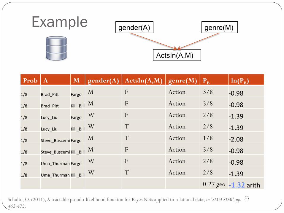
Example
Prob A M gender(A) ActsIn(A,M) genre(M) PB ln(PB)
1/8 Brad_Pi( Fargo M F Action 3/8 -0.98
1/8 Brad_Pi( Kill_Bill M F Action 3/8 -0.98
1/8 Lucy_Liu Fargo W F Action 2/8 -1.39
1/8 Lucy_Liu Kill_Bill W T Action 2/8 -1.39
1/8 Steve_BuscemiFargo M T Action 1/8 -2.08
1/8 Steve_BuscemiKill_Bill M F Action 3/8 -0.98
1/8 Uma_ThurmanFargo W F Action 2/8 -0.98
1/8 Uma_ThurmanKill_Bill W T Action 2/8 -1.390.27 geo -1.32arith
Schulte, O. (2011), A tractable pseudo-likelihood function for Bayes Nets applied to relational data, in 'SIAM SDM', pp. 462-473.
gender(A)
ActsIn(A,M)
genre(M)
38
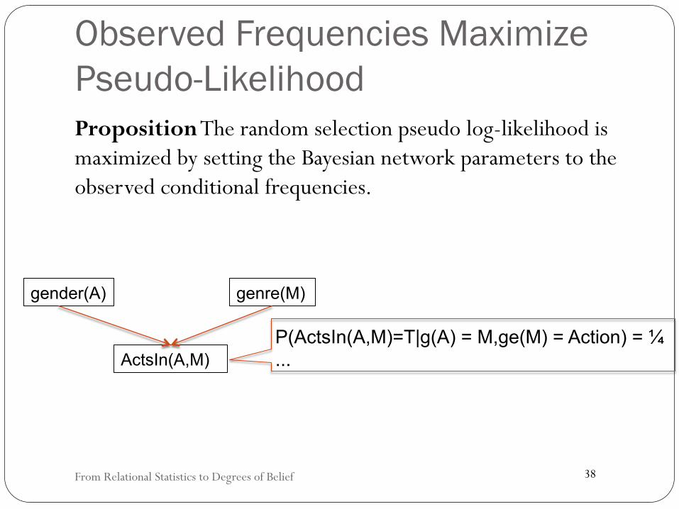
Observed Frequencies Maximize Pseudo-Likelihood Proposition The random selection pseudo log-likelihood is maximized by setting the Bayesian network parameters to the observed conditional frequencies.
From Relational Statistics to Degrees of Belief
gender(A)
ActsIn(A,M)
genre(M)
P(ActsIn(A,M)=T|g(A) = M,ge(M) = Action) = ¼ ...
39
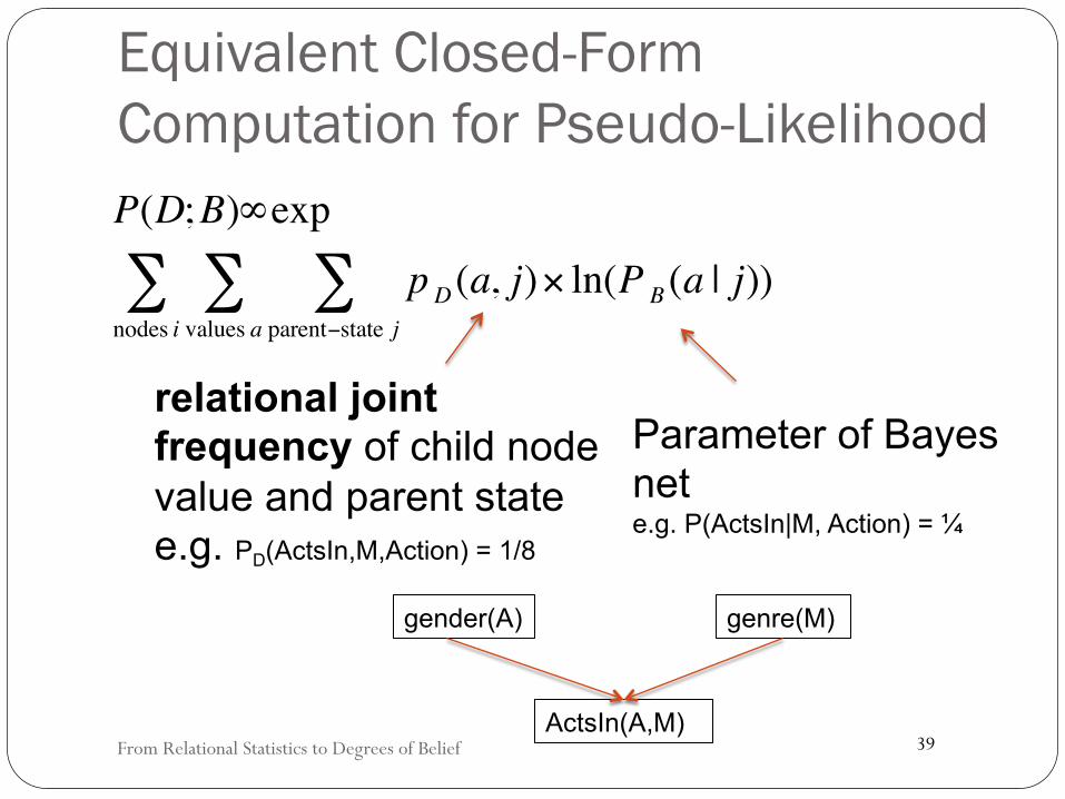
Equivalent Closed-Form Computation for Pseudo-Likelihood
From Relational Statistics to Degrees of Belief
P(D;B)∞exp
pD (a, j)× ln(P B (a | j))parent−state j∑
values a∑
nodes i∑
relational joint frequency of child node value and parent state e.g. PD(ActsIn,M,Action) = 1/8
Parameter of Bayes net e.g. P(ActsIn|M, Action) = ¼
gender(A)
ActsIn(A,M)
genre(M)
Parameter Learning Maximum Likelihood Estimation
From Relational Statistics to Degrees of Belief
41
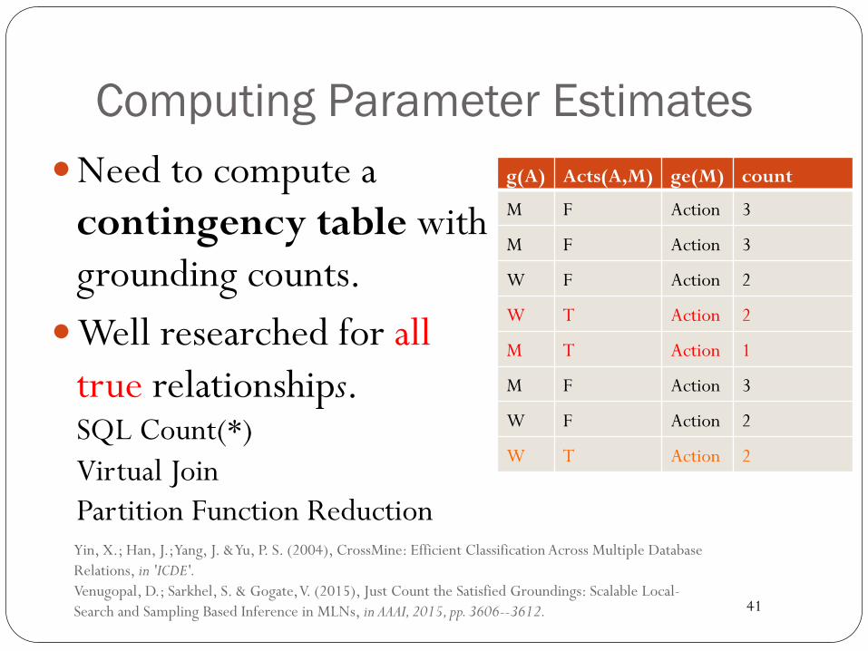
Computing Parameter Estimates � Need to compute a
contingency table with grounding counts.
� Well researched for all true relationships. SQL Count(*) Virtual Join Partition Function Reduction
Yin, X.; Han, J.; Yang, J. & Yu, P. S. (2004), CrossMine: Efficient Classification Across Multiple Database Relations, in 'ICDE'. Venugopal, D.; Sarkhel, S. & Gogate, V. (2015), Just Count the Satisfied Groundings: Scalable Local-Search and Sampling Based Inference in MLNs, in AAAI, 2015, pp. 3606--3612.
g(A) Acts(A,M) ge(M) count
M F Action 3
M F Action 3
W F Action 2
W T Action 2
M T Action 1
M F Action 3
W F Action 2
W T Action 2
42
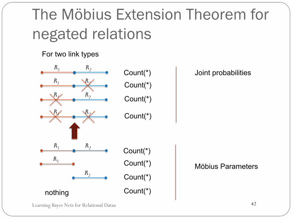
The Möbius Extension Theorem for negated relations
Learning Bayes Nets for Relational Dataa
R1 R2 Count(*) R1 R2 Count(*) R1 R2 Count(*)
R1 R2 Count(*)
For two link types
R1 R2 Count(*) R1 Count(*)
R2 Count(*)
Count(*) nothing
Joint probabilities
Möbius Parameters
43
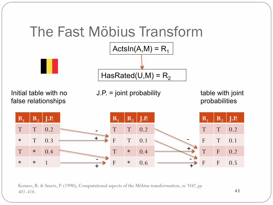
The Fast Möbius Transform
R1 R2 J.P.
T T 0.2
* T 0.3
T * 0.4
* * 1
Kennes, R. & Smets, P. (1990), Computational aspects of the Möbius transformation, in 'UAI', pp. 401-416.
Initial table with no false relationships
R1 R2 J.P.
T T 0.2
F T 0.1
T * 0.4
F * 0.6
R1 R2 J.P.
T T 0.2
F T 0.1
T F 0.2
F F 0.5
+ -
+ -
+ -
+ -
table with joint probabilities
J.P. = joint probability
HasRated(U,M) = R2
ActsIn(A,M) = R1
44
Using Presence and Absence of Relationships � Fast Möbius Transform è almost free computationally! � Allows us to find correlations with relationships.
� e.g. users who search for an item on-line also watch a video about it.
� Relationship variables selected by standard data mining approaches (Qian et al 2014). � Interesting Association Rules. � Feature Selection Metrics.
Qian, Z.; Schulte, O. & Sun, Y. (2014), Computing Multi-Relational Sufficient Statistics for Large Databases, in 'Computational Intelligence and Knowledge Management (CIKM)', pp. 1249--1258.
45
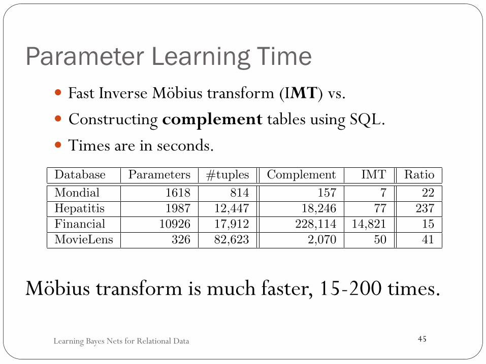
Parameter Learning Time � Fast Inverse Möbius transform (IMT) vs. � Constructing complement tables using SQL. � Times are in seconds.
Learning Bayes Nets for Relational Data
Modelling Relational Statistics With Bayes Nets
Figure 3. The estimates of conditional probability parameters, averaged over 10 random subdatabases and all BN param-eters. Error (absolute di�erence) in conditional probability estimates. The median observation is the red center line andthe box comprises 75% of the observed values. The whisker indicates the maximum acceptable value (1.5 IQR upper).
Table 1. Learning time results (sec) for the Mobius trans-form vs. constructing complement tables. For eachdatabase, we show the number of tuples, and of param-eters in the fixed Bayes net structure.
Database Parameters #tuples Complement IMT Ratio
Mondial 1618 814 157 7 22Hepatitis 1987 12,447 18,246 77 237Financial 10926 17,912 228,114 14,821 15MovieLens 326 82,623 2,070 50 41
then estimated the complete-population frequenciesfrom partial-population data. A fractional samplesize parameter is uniform across tables and databases.We employed standard subgraph subsampling (Frank,1977; Khosravi et al., 2010), which selects entities uni-formly at random and restricts the relationship tuplesin each subdatabase to those that involve only the se-lected entities.
Figure 3 illustrates that with increasing sample size,MPLE estimates approach the true value in all cases.Even for the smaller sample sizes, the median erroris close to 0, confirming that most estimates are veryclose to correct. As the box plots show, the 3rd errorquartile of estimates is bound within 10% on Mondial,the worst case, and within less than 5% on the otherdatasets.
6.4. Inference
The basic inference task for Bayes nets is answeringprobabilistic queries. If the given Bayes net struc-ture is an I-map of the true distribution, then correctparameter values lead to correct predictions. Thusthe performance on queries has been used to evalu-ate parameter learning. We randomly generate queriesfor each dataset according to the following proce-dure. First, choose a target node V 100 times, and go
through each possible value a of V such that P (V = a)is the probability to be predicted. For each value a,choose the number k of conditioning variables, rangingfrom 1 to 3. Select k variables V1, . . . , Vk and corre-sponding values a1, . . . , ak. The query to be answeredis then P (V = a|V1 = a1, . . . , Vk = ak). An examplequery could be
P (Int(S ) = high|Registered(S ,C ) = T , di� (C ) = high).
This asks for the number of student-course pairs witha highly intelligent student, out of the class of student-course pairs where the student is registered in thecourse and the course is di�cult.
As in (Getoor et al., 2001), we evaluate queries af-ter learning parameter values on the entire database.Thus the BN is viewed as a statistical summary of thedata rather than generalizing from a sample. BN in-ference is carried out using the Approximate Updaterin CMU’s Tetrad program. Figure 4 shows that theaccuracy of Bayes net query estimates is high. Wealso compared the runtime cost of performing modelinference vs. estimating query sizes using SQL, butcannot show the details due to lack of space. Basi-cally, model inferences are substantially faster, becausefor larger databases, the cost of data access is muchgreater than the CPU cost of inference computations;see also (Getoor et al., 2001). For queries that involvenegated relations, model inference is faster than den-sity estimation from data by orders of magnitude.
7. Conclusion
We introduced a new semantics for ParametrizedBayes nets as models of class-level statistics in a re-lational structure. For parameter learning we uti-lized the empirical database frequencies, which can befeasibly computed using the Mobius transform, evenfor frequencies concerning negated links. In evalu-ation on four benchmark databases, the maximum
Möbius transform is much faster, 15-200 times.
Structure Learning: Lattice Search
From Relational Statistics to Degrees of Belief
47
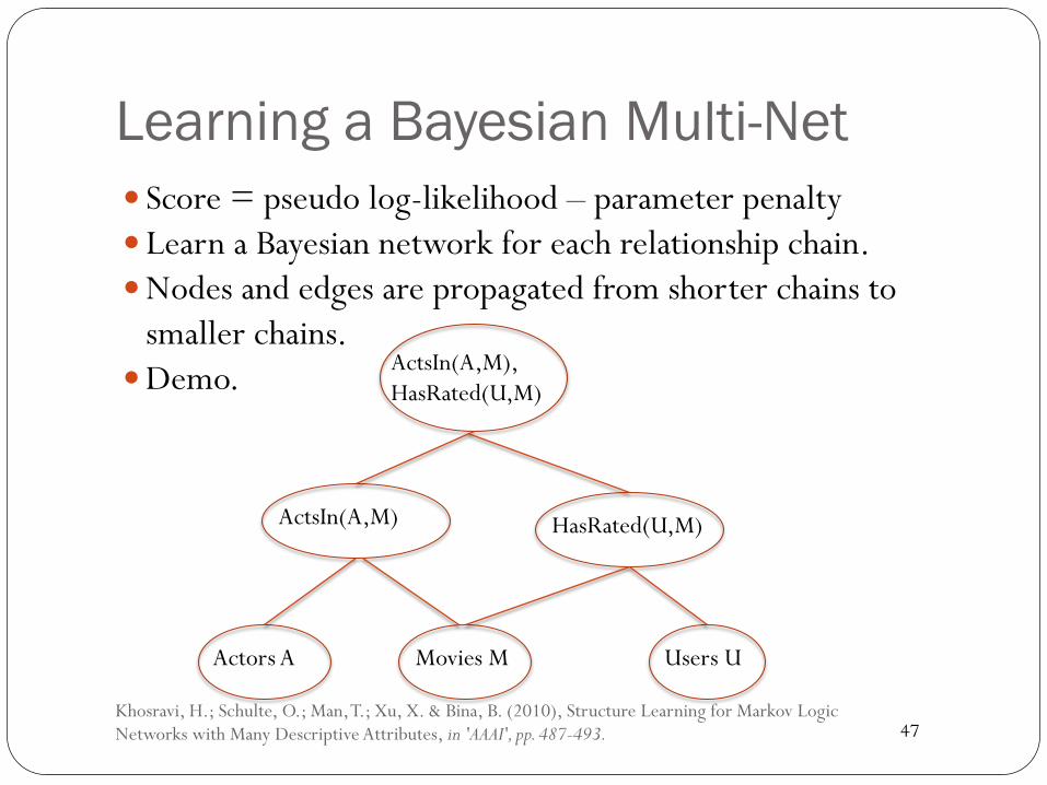
Learning a Bayesian Multi-Net � Score = pseudo log-likelihood – parameter penalty � Learn a Bayesian network for each relationship chain. � Nodes and edges are propagated from shorter chains to
smaller chains. � Demo.
Khosravi, H.; Schulte, O.; Man, T.; Xu, X. & Bina, B. (2010), Structure Learning for Markov Logic Networks with Many Descriptive Attributes, in 'AAAI', pp. 487-493.
Actors A Movies M Users U
ActsIn(A,M) HasRated(U,M)
ActsIn(A,M), HasRated(U,M)
48
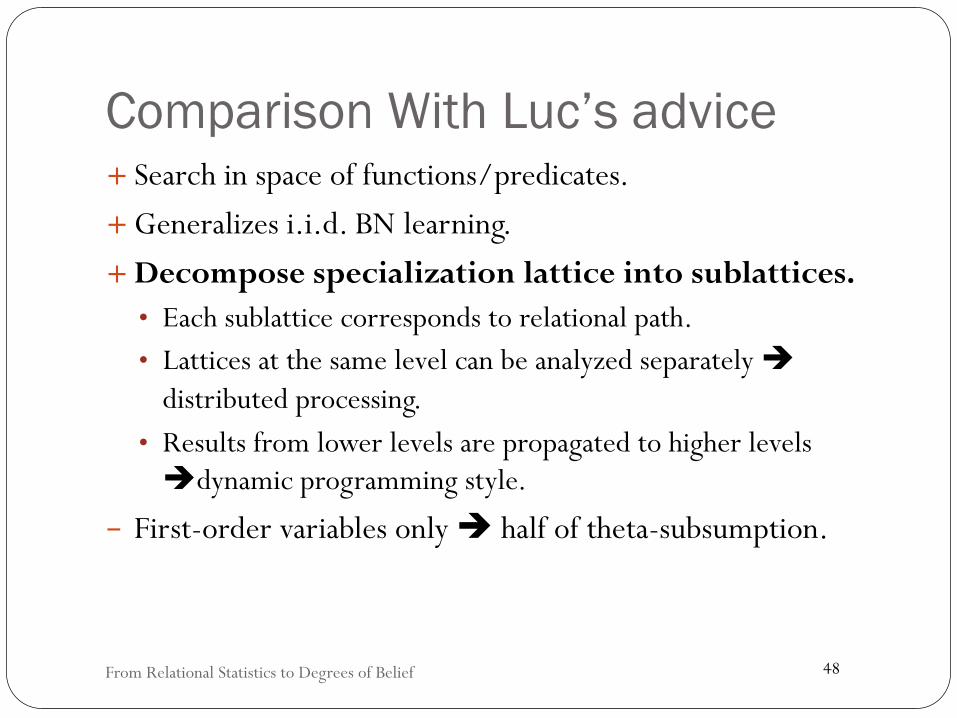
Comparison With Luc’s advice + Search in space of functions/predicates. + Generalizes i.i.d. BN learning. + Decompose specialization lattice into sublattices.
• Each sublattice corresponds to relational path. • Lattices at the same level can be analyzed separately è
distributed processing. • Results from lower levels are propagated to higher levels èdynamic programming style.
- First-order variables only è half of theta-subsumption.
From Relational Statistics to Degrees of Belief
49
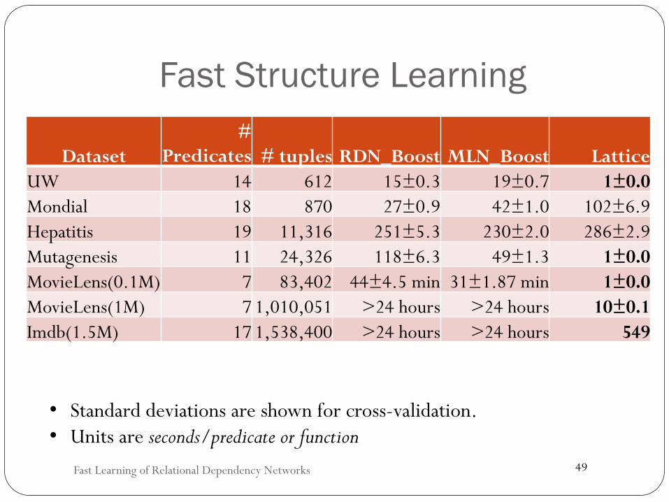
Fast Structure Learning
Dataset#
Predicates # tuplesRDN_BoostMLN_Boost LatticeUW 14 612 15±0.3 19±0.7 1±0.0Mondial 18 870 27±0.9 42±1.0 102±6.9Hepatitis 19 11,316 251±5.3 230±2.0 286±2.9Mutagenesis 11 24,326 118±6.3 49±1.3 1±0.0MovieLens(0.1M) 7 83,402 44±4.5 min 31±1.87 min 1±0.0MovieLens(1M) 7 1,010,051 >24 hours >24 hours 10±0.1Imdb(1.5M) 17 1,538,400 >24 hours >24 hours 549
• Standard deviations are shown for cross-validation. • Units are seconds/predicate or function
Fast Learning of Relational Dependency Networks
From Relational Statistics to Degrees of Belief
Bayesian Network Model for Relational Frequencies
Relational Classifier Dependency Network
Structure and Parameter Learning
New Log-linear Model
51
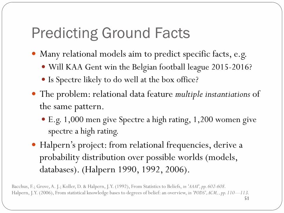
Predicting Ground Facts � Many relational models aim to predict specific facts, e.g.
� Will KAA Gent win the Belgian football league 2015-2016? � Is Spectre likely to do well at the box office?
� The problem: relational data feature multiple instantiations of the same pattern. � E.g. 1,000 men give Spectre a high rating, 1,200 women give
spectre a high rating.
� Halpern’s project: from relational frequencies, derive a probability distribution over possible worlds (models, databases). (Halpern 1990, 1992, 2006).
Bacchus, F.; Grove, A. J.; Koller, D. & Halpern, J. Y. (1992), From Statistics to Beliefs, in 'AAAI', pp. 602-608. Halpern, J. Y. (2006), From statistical knowledge bases to degrees of belief: an overview, in 'PODS', ACM, , pp. 110—113.
52
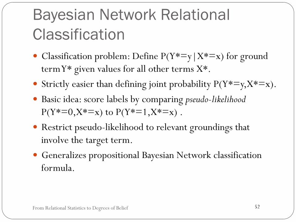
Bayesian Network Relational Classification � Classification problem: Define P(Y*=y|X*=x) for ground
term Y* given values for all other terms X*. � Strictly easier than defining joint probability P(Y*=y,X*=x). � Basic idea: score labels by comparing pseudo-likelihood
P(Y*=0,X*=x) to P(Y*=1,X*=x) . � Restrict pseudo-likelihood to relevant groundings that
involve the target term. � Generalizes propositional Bayesian Network classification
formula.
From Relational Statistics to Degrees of Belief
53
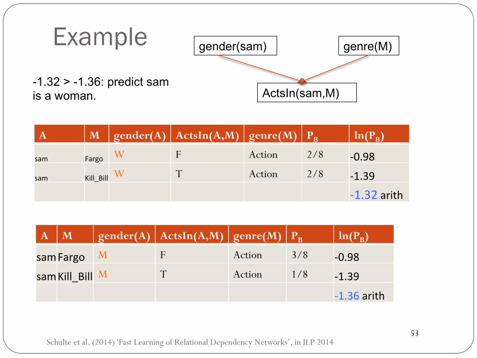
Example
A M gender(A) ActsIn(A,M) genre(M) PB ln(PB)
sam Fargo W F Action 2/8 -0.98
sam Kill_Bill W T Action 2/8 -1.39
-1.32arith
Schulte et al. (2014) ‘Fast Learning of Relational Dependency Networks’, in ILP 2014
gender(sam)
ActsIn(sam,M)
genre(M)
-1.32 > -1.36: predict sam is a woman.
A M gender(A) ActsIn(A,M) genre(M) PB ln(PB)
samFargo M F Action 3/8 -0.98
samKill_Bill M T Action 1/8 -1.39
-1.36arith
54
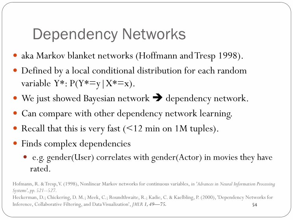
Dependency Networks � aka Markov blanket networks (Hoffmann and Tresp 1998). � Defined by a local conditional distribution for each random
variable Y*: P(Y*=y|X*=x). � We just showed Bayesian network è dependency network. � Can compare with other dependency network learning. � Recall that this is very fast (<12 min on 1M tuples). � Finds complex dependencies
� e.g. gender(User) correlates with gender(Actor) in movies they have rated.
Hofmann, R. & Tresp, V. (1998), Nonlinear Markov networks for continuous variables, in 'Advances in Neural Information Processing Systems', pp. 521--527. Heckerman, D.; Chickering, D. M.; Meek, C.; Roundthwaite, R.; Kadie, C. & Kaelbling, P. (2000), 'Dependency Networks for Inference, Collaborative Filtering, and Data Visualization', JMLR 1, 49—75.
55
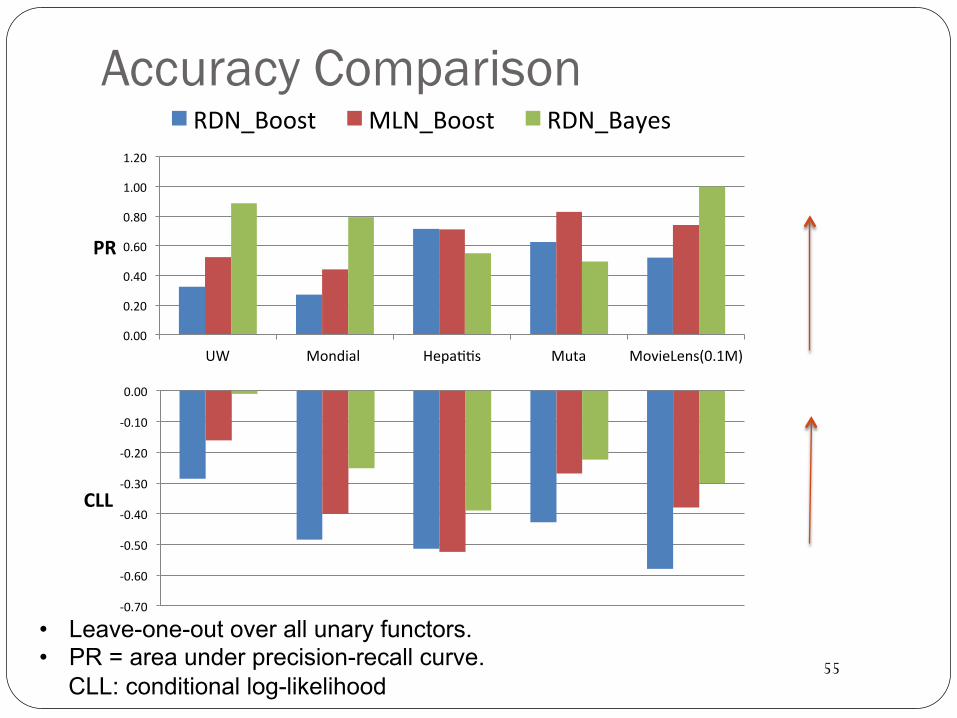
Accuracy Comparison
-0.70
-0.60
-0.50
-0.40
-0.30
-0.20
-0.10
0.00
CLL
0.00
0.20
0.40
0.60
0.80
1.00
1.20
UW Mondial HepaNNs Muta MovieLens(0.1M)
PR
RDN_Boost MLN_Boost RDN_Bayes
• Leave-one-out over all unary functors. • PR = area under precision-recall curve.
CLL: conditional log-likelihood
Model-Based Unsupervised Relational Outlier Detection
From Relational Statistics to Degrees of Belief
57
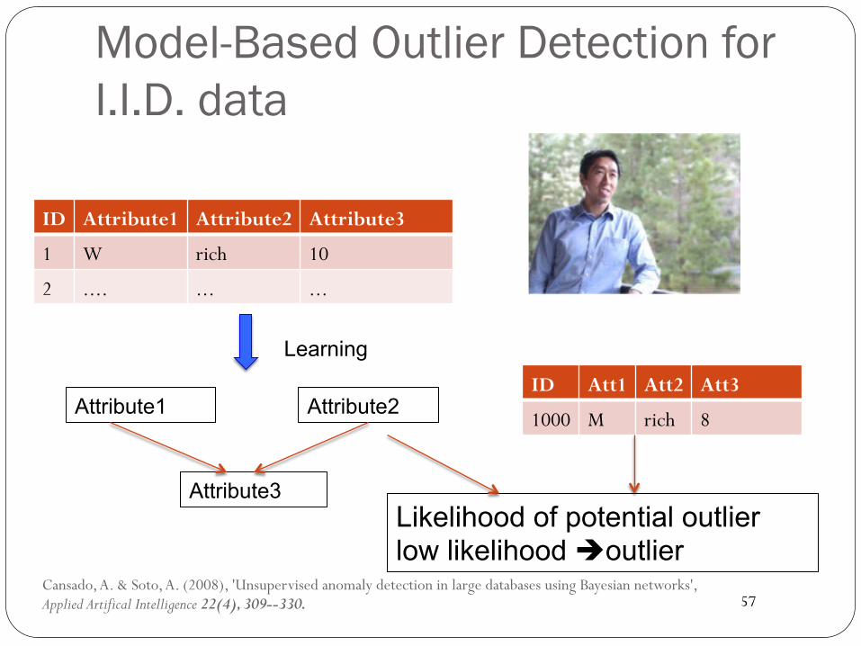
Model-Based Outlier Detection for I.I.D. data
ID Att1 Att2 Att3
1000 M rich 8
Cansado, A. & Soto, A. (2008), 'Unsupervised anomaly detection in large databases using Bayesian networks', Applied Artifical Intelligence 22(4), 309--330.
Attribute1
Attribute3
Attribute2
Learning
ID Attribute1 Attribute2 Attribute3
1 W rich 10
2 .... ... ...
Likelihood of potential outlier low likelihood èoutlier
58
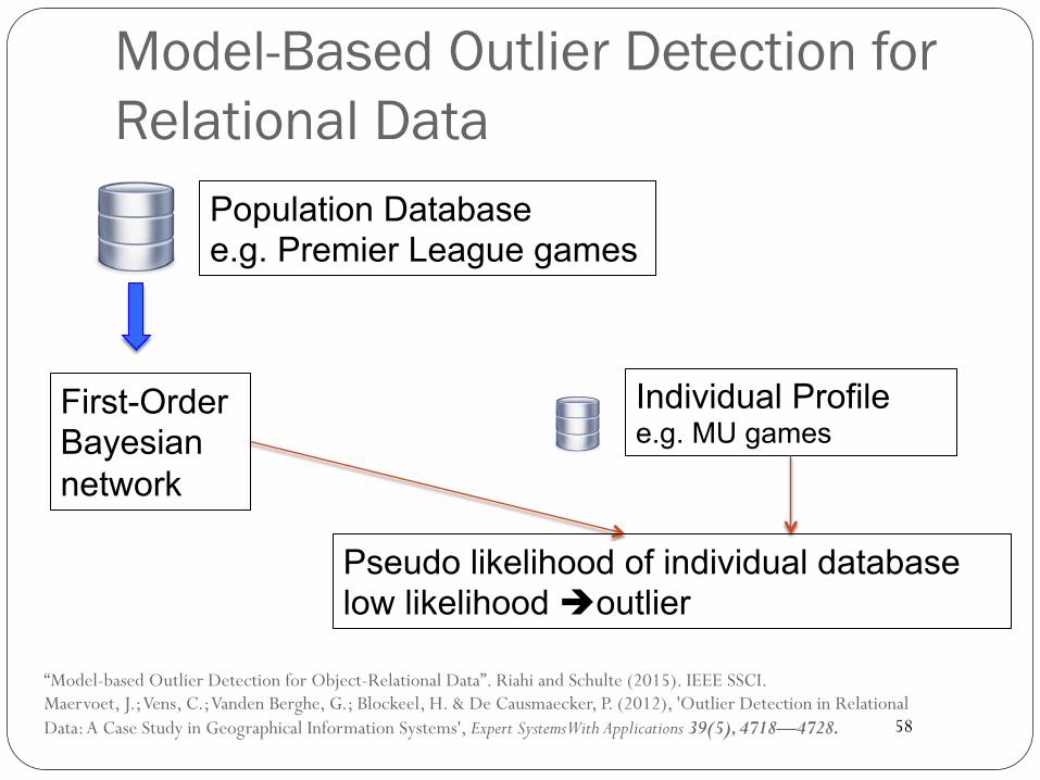
Model-Based Outlier Detection for Relational Data
“Model-based Outlier Detection for Object-Relational Data”. Riahi and Schulte (2015). IEEE SSCI. Maervoet, J.; Vens, C.; Vanden Berghe, G.; Blockeel, H. & De Causmaecker, P. (2012), 'Outlier Detection in Relational Data: A Case Study in Geographical Information Systems', Expert Systems With Applications 39(5), 4718—4728.
Individual Profile e.g. MU games
First-Order Bayesian network
Pseudo likelihood of individual database low likelihood èoutlier
Population Database e.g. Premier League games
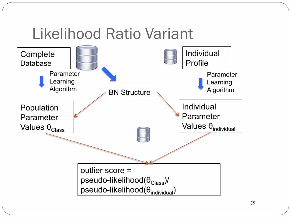
59
Likelihood Ratio Variant Complete Database
Population Parameter Values θClass
outlier score = pseudo-likelihood(θClass)/ pseudo-likelihood(θindividual)
Individual Profile
Individual Parameter Values θindividual
Parameter Learning Algorithm
Parameter Learning Algorithm BN Structure
60
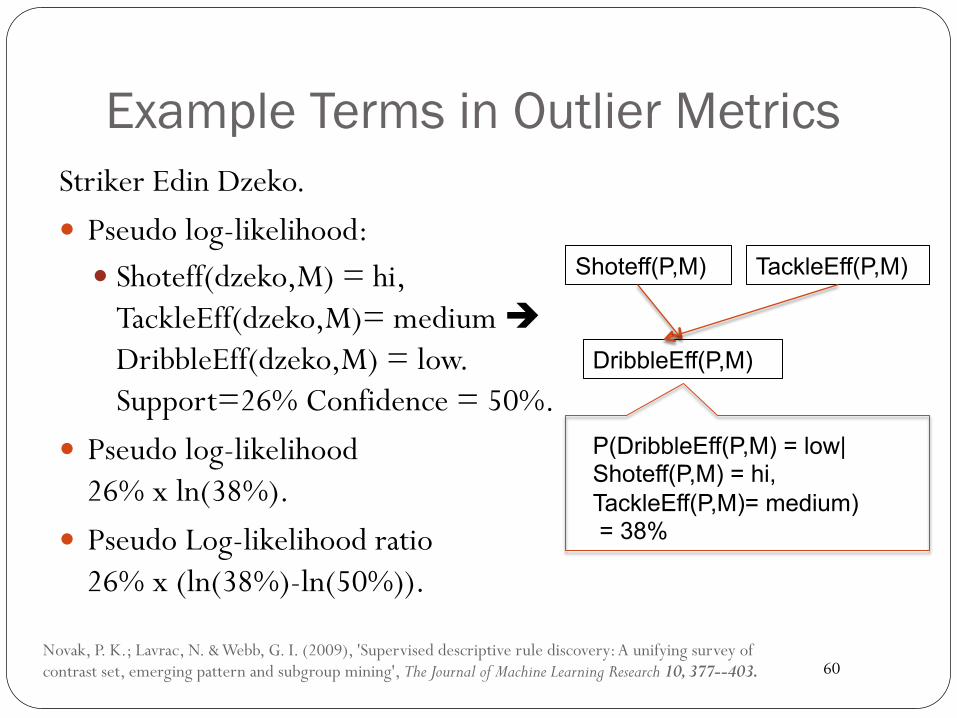
Example Terms in Outlier Metrics Striker Edin Dzeko. � Pseudo log-likelihood:
� Shoteff(dzeko,M) = hi, TackleEff(dzeko,M)= medium è DribbleEff(dzeko,M) = low. Support=26% Confidence = 50%.
� Pseudo log-likelihood 26% x ln(38%).
� Pseudo Log-likelihood ratio 26% x (ln(38%)-ln(50%)).
Novak, P. K.; Lavrac, N. & Webb, G. I. (2009), 'Supervised descriptive rule discovery: A unifying survey of contrast set, emerging pattern and subgroup mining', The Journal of Machine Learning Research 10, 377--403.
Shoteff(P,M)
DribbleEff(P,M)
TackleEff(P,M)
P(DribbleEff(P,M) = low| Shoteff(P,M) = hi, TackleEff(P,M)= medium) = 38%
61
Interpretable (and Accurate)
Riahi, S. and Schulte, O. (2015). ‘Model-based Outlier Detection for Object-Relational Data’ IEEE Symposium Series on Computing Intelligence. Forthcoming. 61
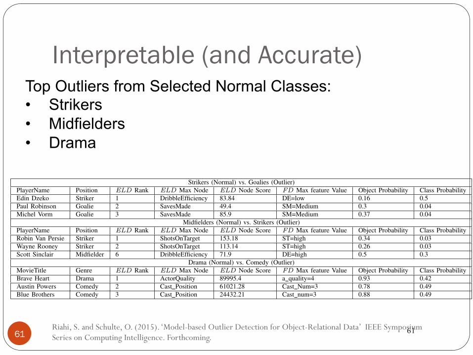
Top Outliers from Selected Normal Classes: • Strikers • Midfielders • Drama TABLE XI. CASE STUDY FOR THE TOP OUTLIERS RETURNED BY THE LOG-LIKELIHOOD DISTANCE SCORE ELD
Strikers (Normal) vs. Goalies (Outlier)PlayerName Position ELD Rank ELD Max Node ELD Node Score FD Max feature Value Object Probability Class ProbabilityEdin Dzeko Striker 1 DribbleEfficiency 83.84 DE=low 0.16 0.5Paul Robinson Goalie 2 SavesMade 49.4 SM=Medium 0.3 0.04Michel Vorm Goalie 3 SavesMade 85.9 SM=Medium 0.37 0.04
Midfielders (Normal) vs. Strikers (Outlier)PlayerName Position ELD Rank ELD Max Node ELD Node Score FD Max feature Value Object Probability Class ProbabilityRobin Van Persie Striker 1 ShotsOnTarget 153.18 ST=high 0.34 0.03Wayne Rooney Striker 2 ShotsOnTarget 113.14 ST=high 0.26 0.03Scott Sinclair Midfielder 6 DribbleEfficiency 71.9 DE=high 0.5 0.3
Drama (Normal) vs. Comedy (Outlier)MovieTitle Genre ELD Rank ELD Max Node ELD Node Score FD Max feature Value Object Probability Class ProbabilityBrave Heart Drama 1 ActorQuality 89995.4 a quality=4 0.93 0.42Austin Powers Comedy 2 Cast Position 61021.28 Cast Num=3 0.78 0.49Blue Brothers Comedy 3 Cast Position 24432.21 Cast num=3 0.88 0.49
There are several avenues for future work. (i) A limitationof our current approach is that it ranks potential outliers, butdoes not set a threshold for a binary identification of outliervs. non-outlier. (ii) Our divergence uses expected L1-distancefor interpretability, but other distance scores like L2 could beinvestigated as well. (iii) Extending the expected L1-distancefor continuous features is a useful addition.
In sum, outlier metrics based on model likelihoods are anew type of structured outlier score for object-relational data.Our evaluation indicates that this model-based score providesinformative, interpretable, and accurate rankings of objects aspotential outliers.
ACKNOWLEDGEMENT
This work was supported by a Discovery Grant from theNational Sciences and Engineering Council of Canada.
REFERENCES
[1] E. Achtert, H. Kriegel, E. Schubert, and A. Zimek. Interactive datamining with 3d-parallel coordinate trees. In Proceedings of the 2013ACM SIGMOD, New York, NY, USA, 2013.
[2] C. Aggarwal. Outlier Analysis. Springer New York, 2013.[3] F. Angiulli, G. Greco, and L. Palopoli. Outlier detection by logic
programming. ACM Transactions on Computer Logic, 2004.[4] M. Breunig, H.-P. Kriegel, R. T. Ng, and J. Sander. Lof: Identifying
density-based local outliers. In Proceedings of ACM SIGMOD, 2000.[5] A. Cansado and A. Soto. Unsupervised anomaly detection in large
databases using Bayes Nets. Appllied Artificial Intelligence, 2008.[6] L. de Campos. A scoring function for learning Bayes nets based on
mutual information and conditional independence tests. Journal ofMachine learning Research, 2006.
[7] P. Domingos and D. Lowd. Markov Logic: An Interface Layer forArtificial Intelligence. Morgan and Claypool Publishers, 2009.
[8] P. A. Flach. Knowledge representation for inductive learning. InSymbolic and Quantitative Approaches to Reasoning and Uncertainty,pages 160–167. Springer, 1999.
[9] J. Gao, F. Liang, W. Fan, Y. Wang, and J. Han. On community outliersand their detection in information network. In Proceedings of ACMSIGKDD, 2010.
[10] L. Getoor and B. Taskar. Introduction to statistical relational learning.MIT Press, 2007.
[11] Internet Movie Database. Internet movie database. [Online]. Available:URL = http://www.imdb.com/.
[12] H. Khosravi, T. Man, J. Hu, E. Gao, and O. Schulte. Learn andjoin algorithm code. [Online]. Available: URL = http://www.cs.sfu.ca/⇠oschulte/jbn/.
[13] A. Kimmig, L. Mihalkova, and L. Getoor. Lifted graphical models: asurvey. Computing Research Repository, 2014.
[14] J. L. Koh, M. L. Lee, W. Hsu, and W. T. Ang. Correlation-based attributeoutlier detection in XML. In Proceedings of ICDE. IEEE 24th, 2008.
[15] D. Koller and A. Pfeffer. Object-oriented Bayes nets. In Proceedingsof UAI, 1997.
[16] J. Maervoet, C. Vens, G. Vanden Berghe, H. Blockeel, and P. De Caus-maecker. Outlier detection in relational data: A case study. ExpertSystem Applications, 2012.
[17] MCFC Analytics. The premier league dataset. [Online]. Available:URL = http://www.mcfc.co.uk/Home/MCFCAnalytics.
[18] E. Muller, I. Assent, P. Iglesias, Y. Mulle, and K. Bohm. Outlier rankingvia subspace analysis in multiple views of the data. In Proceedings ofICDM, 2012.
[19] P. K. Novak, G. I. Webb, and S. Wrobel. Supervised descriptive rulediscovery: A unifying survey of contrast set, emerging pattern andsubgroup mining. Journal of Machine Learning Research, 2009.
[20] J. Pearl. Probabilistic Reasoning in Intelligent Systems. MorganKaufmann, 1988.
[21] V. Peralta. Extraction and Integration of MovieLens and IMDb.Technical report, APDM project, 2007.
[22] D. Poole. First-order probabilistic inference. In Proceedings of IJCAI,2003.
[23] S. Ramaswamy, R. Rastogi, and K. Shim. Efficient algorithms formining outliers from large data sets. SIGMOD, 2000.
[24] F. Riahi and O. Schulte. Codes and Datasets. [Online]. Available:.ftp://ftp.fas.sfu.ca/pub/cs/oschulte/CodesAndDatasets/, 2015.
[25] S. Sarawagi, R. Agrawal, and N. Megiddo. Discovery-driven explorationof OLAP data cubes. In Proceedings of International Conference onExtending Database Technology. Springer-Verlag, 1998.
[26] O. Schulte. A tractable pseudo-likelihood function for Bayes netsapplied to relational data. In Proceedings of SIAM SDM, 2011.
[27] O. Schulte and H. Khosravi. Learning graphical models for relationaldata via lattice search. Journal of Machine Learning, 2012.
[28] G. Tang, J. Bailey, J. Pei, and G. Dong. Mining multidimensionalcontextual outliers from categorical relational data. In Proceedings ofSSDBM, 2013.
[29] S. Tuffery. Data Mining and Statistics for Decision Making. WileySeries in Computational Statistics, 2011.
Summary, Review, Open Problems
From Relational Statistics to Degrees of Belief
63
Random Selection Semantics for First-Order Logic � First-order variables and first-order terms are viewed as
random variables. � Associates relational frequency with each first-order formula.
From Relational Statistics to Degrees of Belief
Joe Halpern Fahim Bacchus
64
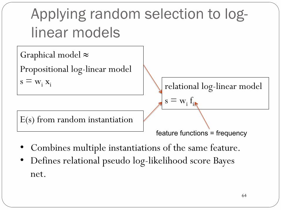
Applying random selection to log-linear models
Graphical model ≈ Propositional log-linear model s = wi xi
E(s) from random instantiation
relational log-linear model s = wi fi
feature functions = frequency
• Combines multiple instantiations of the same feature. • Defines relational pseudo log-likelihood score Bayes
net.
65
Log-linear Models With Proportions � Frequencies are on the same scale [0,1]: addresses “ill-
conditioning” (Lowd and Domingos 2007). � Surprisingly expressive: can “simulate” combining rules
(Kazemi et al. 2014). � Also effective for dependency networks with hybrid data
types (Ravkic, Ramon, Davis 2015). � Random selection semantics provides a theoretical
foundation.
Lowd, D. & Domingos, P. (2007), Efficient Weight Learning for Markov Logic Networks, in 'PKDD', pp. 200—211. Kazemi, S. M.; Buchman, D.; Kersting, K.; Natarajan, S. & Poole, D. (2014), Relational Logistic Regression, in 'Principles of Knowledge Representation and Reasoning:, KR 2014. Ravkic, I.; Ramon, J. & Davis, J. (2015), 'Learning relational dependency networks in hybrid domains', Machine Learning.
66
Learning results � Random selection pseudo-likelihood score for Bayesian
networks. � Closed-form parameter estimation.
� Fast Möbius transform for computing parameters with negated relationships.
� Structure Learning: Decompose the lattice of relationship chains.
� Fast learning, competitive accuracy for: � modeling relational frequencies. � relational dependency networks. � relational outlier detection.
From Relational Statistics to Degrees of Belief
67
Open Problems � Learning with constants (theta-subsumption). � Generalize model scores like AIC, BIC with positive and
negative relationships. � need to scale penalty terms as well as feature counts.
From Relational Statistics to Degrees of Belief

68
Thank you! � Any questions?
From Relational Statistics to Degrees of Belief