Draft – Please do not cite without authors’ permission

"From Dark to Light: Skin Color and Wages Among African-Americans"

Arthur H. Goldsmith Department of Economics

Washington and Lee University Lexington, VA 24450 Office: (540) 463-8970

Fax: (540) 463-8639 e-mail: GoldsmithA@wlu.edu

Darrick Hamilton

Milano-The Newschool of Management and Urban Policy

New School University 72 Fifth Avenue

New York, NY 10011 Office: (212) 229-5311, ext. 1514

Fax: (212) 229-5335 e-mail: hamiltod@newschool.edu

William Darity, Jr.

Department of Economics University of North Carolina at Chapel Hill

Chapel Hill, NC 27514 Office: (919) 966-2156 Fax: (919) 966-4986

e-mail: darity@unc.edu

I. OVERVIEW

Conventional wisdom in the social sciences holds that there is a fundamental

difference in the construction and understanding of racial categories between most

communities in Latin American countries and most communities in the United States of

America. The standard claim has it that racial distinction is dictated primarily by

phenotype or physical appearance in Latin America and is dictated primarily by genotype

or ancestry in the USA (Rodriguez, 1991 is representative)1 However, recent research is

subverting the sharpness of this alleged conceptual divide (Keith and Herring 1991;

Seltzer and Smith 1991; Falcon 1995; Twine 1998; Hill 2000; and Darity, Dietrich and

Hamilton 2002).

There is an extensive literature examining the influence of race on wages in the

United States and the mechanisms through which race affects wages (see the surveys by

Cain [1986] and Altonji and Blank [1999]). A distinguishing feature of this literature is a

bi-variate race categorization of workers as--black or white--which is consistent with the

conventional wisdom of U.S. racial categorization. This paper offers an alternative

perspective, that the link between wages and race is more complex than the simple bi-

variate rankings with whites at the top. Rather we argue that the wage hierarchy is

characterized by a more gradational ranking with whites at the top and dark skinned blacks

at the bottom.

We offer and test a theory which suggests that as skin shade lightens the wages for

blacks rise. Thus, our theory predicts that the white-black wage gap is greater for darker

skinned blacks than for blacks with lighter skin. We estimate two sets of models, one

based on a bi-variate grouping of blacks and whites and a second set based on a grouping

of whites and blacks disaggregated based on their skin shade. We refer to the first set of

models as the “one drop” models, where “one-drop” is used figuratively to connote

individuals that have at least “one drop” of black blood, and the second set as the

“rainbow” models, where the “rainbow” metaphor is used to connote imagery of a range

of categories based on skin shade. We estimate the two sets of wage equations to

document the link between skin shade and wages as well as the shortcoming of

characterising race as either black or white rather than on a continuum from light to dark.

1 Phenotype entails the collective dimensions of a person’s physical appearance including factors such as complexion, facial dimensions, and hair texture which are expected to be unrelated to an individual’s productivity.

2

We begin by constructing a hypothesis which we refer to as a “preference for

whiteness” as an explanation for wage gaps based on skin shade. This hypothesis is

founded on insights from social psychology (Tajfel and Turner, 1986; Campbell, 1965;

Fisk and Ruscher, 1993) and anthropology (Sumner, 1906). The theory rests on three

cornerstones: First, social categorization is a fundamental cognitive process leading to

“in-groups” and ”out-groups,” where “out-groups” are exposed to prejudicial attitudes and

biased judgements and “in-group” members receive preferential treatment. Second,

socialization patterns and the structure of rewards in the USA have lead to “whiteness” as

a defining attribute of the in-group; lighter skin can give an individual greater proximity to

the benefits associated with whiteness, regardless of their racial classification. Third, in-

group members are ascribed higher social status, which also leads to preferential treatment

of workers possessing the characteristics of the in-group. Thus, preferential treatment of

in-group characteristics is expected to foster higher wages for those blacks with lighter

skin relative to those with darker skin because of their phenotypical proximity to the

preferred white workers.2

A strength of this study is that we use two separate, independently assembled, data

sets the National Survey of Black Americans (NSBA, 1979) and the Multi City Study of

Urban Inequality (MCSUI, 1992) which categorize black respondents by their skin shade.3

Motivated by the theory of white preference we test hypotheses that shed light on two

questions. First, does the inter-racial (white-black) and intra-racial wage gap widen as the

skin shade of the black workers darkens? Second, are the factors that contribute to wages

treated more favourably for workers with lighter skin shade? To answer this later question,

we decompose inter-racial and intra-racial wage gaps to determine the size of the gap due

to differences in the amounts of the characteristics that contribute to wages and differences

in the valuation of these characteristics.

The remainder of this paper is organized as follows. The theory of preference for

whiteness is developed and presented in Section II. In Section III, the data we use from

the Multi City Study of Urban Inequality is described, along with the methodology

employed to estimate skin shade differences and bi-variate racial differences in wages.

Our findings on the link between race and wages generated by estimating skin shade and

bi-variate wage equations, controlling for a wide range of productivity linked personal

2 We are using skin shade as a proxy for one of many “white characteristics.” 3 We focus on males because sorting between the effects of race/skin color and gender requires a separate study.

3

characteristics, demographic factors, family attributes as a youth and neighborhood

descriptors, are presented in Section IV. This section provides evidence on whether inter-

racial and intra-racial wage gaps expand as skin shade differences between the groups

widen. The robustness of our findings on the link between intra-racial wage differences

and skin shade is explored by using a second data set the National Survey of Black

Americans (NSBA). Section IV contains these results along with a description of the

NSBA data. In Section V we decompose inter-racial and intra-racial wage gaps, using both

data sets, to identify how racial wage gaps are influenced by differences between groups in

the levels of wage related characterises and differences in the treatment or valuation of

these characteristics. This exercise reveals if favorable treatment of lighter skinned

workers is a key source of racial wage differences as predicted by the theory of a

preference for whiteness. Concluding observations appear in Section VI.

II. PREFERENCE FOR WHITENESS AND WAGES

A. In Groups, Out Groups and Skin Shade

Social psychologists believe that human categorization is a fundamental

cognitive process. The general tendency of human beings to differentiate themselves

according to group membership was documented early in the previous century in

extensive anthropological observations compiled by Sumner (1906). Sumner coined the

distinction between in-group and out-group, and suggested that preference for in-groups

over out-groups is a universal characteristic of social existence.

A convention has emerged in representing in-group and out-group status along the

racial axis on a bi-variate scale with white as the in-group and not white as the out-group

(a convention based on the “one drop rule”). Because of strong and persistent evidence of

comparatively preferential treatment of blacks with lighter complexions both by whites

and blacks, we depart from this convention. We believe that patterns of socialization in the

USA also are consistent with a gradational model of in-group and out-group with regard to

phenotype. In this framework, lightness begets access to in-group privileges, rather than

whiteness alone. It follows then, that if having “white” skin shade is an attribute of the in-

group, light skin blacks should receive greater societal rewards than dark skin blacks,

because of their proximity to the more socially desired skin color of the in-group.

We recognize that there are many characteristics and traits besides skin color that

are associated with the white in-group. Examples are diction, accents, mannerisms, hair

texture, clothing, residence, naming practices, and the list continues. We use skin shade as

4

the proxy for possessing in-group characteristics in part because this in-group feature is

available in our data sets.

Moreover, skin shade is a salient feature that distinguishes minorities from

members of the majority population in the United States. According to Hall (1995) many

African-Americans have adopted the dominant culture’s preference for lighter skin.4 The

motivation to pursue or value lightness is a response in part to the behaviour of whites.5

Hall calls efforts by blacks to make their skin lighter through the use of “beauty” creams

and folk preparations, to gain status, the “bleaching syndrome.”6

Black history provides considerable evidence that the skin shade of African

Americans has exerted powerful and persistent influences on attitudes toward and

treatment of black persons within both white and black communities (for recent reviews

see Neal and Wilson, 1989; Gatewood, 1988; Hughes and Hertel, 1990; Okazawa-Rey,

Robinson, and Ward, 1987). During the era of slavery, light complexioned blacks, often

the offspring of white slave owners and enslaved Africans, were given preferential

treatment through assignment to housework while darker skinned blacks were typically

assigned to outdoor or hard-labor tasks (Keith and Herring, 1991). Moreover, skin shade

played a profound role in the acquisition of social status for black Americans following

the abolition of slavery.7

Maddox and Gray (2002) report that both whites and blacks attribute more positive

attributes and greater social status to lighter skinned blacks. In addition, new studies are

emerging that demonstrate a preference for whiteness amongst racial and ethnic minorities.

4 Light skin tone has become a point of reference for the attractiveness of African American females (Okazawa-Rey, Robinson, and Ward, 1987; Neal and Wilson, 1989; Bond and Cash, 1992). African American folk terms developed to describe variations in shin shade generally are complimentary of light skin color (Herskovits, 1968) and include terms such as “high yellow,” “ginger,” “crème,” and “bronze.” 5 W.E.B. DuBois in his “theory of double consciousness” argued that anyone in America whose skin shade did not approximate that of the dominant culture had an incentive to assume a passive social demeanour in order not to further offend, and to thus gain a greater degree of American assimilation. 6 There is international evidence of this preference for whiteness as well. Marketers of skin lightening lotions and creams in Africa, India, the Philippines, and Malaysia promote their products as offering a “fairer complexion.” Despite the health risks associated with the use of lightening lotions, sales remain strong. Repeated use of lightening creams removes the skin’s melanin pigment, leads to skin that is thin, brittle, bruises easily, and is more vulnerable to sunburn and related cancers. Lightening creams promote discoloration and rashes leading to what Ugandan’s call the Pepsi-Mirinda effect--where part of the body is a fiery orange (like a mirinda soda) and part of it (typically in the area of joints) is dark black-green in hue (New Vision, 2001). Nevertheless sales are strong with half of the women in Mali believed to have tried creams many of which are made by Nish manufacturers of the United Kingdom under the brand names Jaribu, Mekako, and Amira. In India, Hindu males exhibit a preference for light skinned brides. In 2003 sales of skin lighteners were $147.36 million in India (Sullivan, 2003). 7 At the turn of the previous century, African Americans” organized “blue vein” societies where a prerequisite for membership included skin tone lighter than a “paper bag” or light enough for visibility of “blue veins.”

5

Darity and Boza (2003) using data drawn from the Latino National Political Survey

(1989-1990) find a majority of persons of either Mexican, Puerto Rican or Cuban descent

self identified as racially white--even if they were identified as dark-skinned by the

interviewers.

2. In-Groups, Out-Groups and Prejudice

Social Identity Theory (Tajfel and Turner, 1979, 1986) is used by

social psychologists to explain why persons belonging to an in-group are prejudiced

toward members of the out-group. In our context, where in-group status is related to skin

shade, Social Identity Theory provides a basis for why both whites and blacks might treat

lighter complexioned blacks better than darker blacks.

Social Identity Theory asserts that people have a fundamental need for self-worth

and self-esteem. An individual’s self-worth or self-esteem is enhanced by their group’s

success and achievements--due to a perception of common fate--that an individual’s

outcomes are linked to their group’s outcomes. Therefore, positive in-group bias is

expected because it can improve the standing of the in-group relative to the comparison

group. Thereby, it contributes to self-worth. According to this theory the mere

categorization of people into two groups, in-groups and out-groups is sufficient to induce

inter-group discrimination where in-group members discriminate against the out-group

and out-group members discriminate against the in-group. We refer to this inter-group

discrimination as the “categorization effect.” The outcomes of the “categorization effect”

may be asymmetric given that one-group may be endowed with greater resources and

power than the other leading to disproportionate effects of each group discriminating

against the other--the in-group may be relatively more effective in discriminating against

the out-group.8

Tajfel and Turner extended their core thesis by suggesting that group status has an

independent and powerful impact on inter-group behaviour which we refer to it as the

“status effect.” Tajfel and Turner argue that if low status group members acknowledge the

superiority of high status group members on the status-related dimension of comparison

(skin shade) then low status group members will show out-group favoritism (i.e.,

favoritism towards the high status group) rather than own-group favouritism. If the “status

8 We are currently working on a theoretical (mathematical) model of inter-group discrimination that explains how certain preconditions can lead to asymmetric outcomes for various groups.

6

effect” is strong enough then darker skinned blacks as well as whites will treat lighter

skinned blacks more favourably.9

Two decades of experimental research by psychologists reviewed by Brewer and

Brown (1999) reveals that social identification with in-groups elicits liking, trust, and

cooperation toward in-group members that are not extended to out-group members.10

Moreover, in bargaining games studied by social psychologists (Commins and Lockwood,

1979; and Turner, 1978) and economists (Ball and Eckel, 1998; Ball, Eckel, Grossman,

and Zame, 2001) participants were found to treat persons better if the other has higher

status than their own. According to Ball et al. (2001), status carries with it privileges and

expectations of entitlement to resources.

The theory of preference for whiteness predicts that the impulse to categorize

workers according to complexion and to confer status on those with lighter skin shade will

lead to favorable treatment and assessment, and hence higher wages, as skin tone becomes

lighter. This gradational perspective on how race influences labor market outcomes raises

an interesting question. How far along the skin shade continuum does the financial benefit

of lightness extend? Is it the case that the wages of light complexioned blacks still fall

short of white wages, but the inter-racial wage gap is less than the gap experienced by

blacks with darker skin shade? Among black workers is there an intra-racial wage gap

based on skin shade? We turn next to a discussion of the data that will be used to explore

these questions.

III. DATA AND METHODOLOGY

A. Data

Data from the National Survey of Black Americans (NSBA) and from the Multi City

Study of Urban Inequality (MSCUI) are used in this study. The Multi City Study of Urban

Inequality is an interview-based survey of close to 9,000 Households and 2,400 Firms

administered in the cities of Los Angeles, Boston, Atlanta, and Detroit beginning in 1992.

MCSUI respondents included whites, blacks, Hispanics, Asians, and persons coded as

“other.” In conducting the Household Survey, from which we use data, attempts were

made to “race match,” by assigning interviewers of a certain race or ethnicity to 9 Evidence from Hagendoorn and Henki (1991), Sachdev and Bourhis (1987), Brown and Abrams (1986), and Van Knippenberg (1978) reveals that when status hierarchy is perceived as stable and legitimate, persons from both in-groups and out-groups evaluate in-group members more favourably. 10 Brewer and Brown (1999) report that people tend to rate their own group more positively than others, even when the groups are artificially constructed and even when they have little reason to expect differences between the groups.

7

respondents of that same race/ethnicity. MCSUI and NSBA interviewers graded

respondents on a salient phenotypical dimension, skin shade, using a Likert scale. Prior to

conducting interviews, the orientation of MCSUI and NSBA interviewers included training

to establish consistency in the coding of respondent skin shade. The NSBA interviewers

used five categories (“very dark,” “dark,” “medium,” “light,” and “very light”) when

coding skin shade, while three categories were used to describe the complexion of blacks

who participated in the MCSUI survey. For analytical and sample size purposes we

collapsed the NSBA data into three categories: light (which includes “very light” and

“light”), medium, and dark (containing “very dark” and “dark”) which conform to the

MCSUI classification scheme.

We restrict the analysis to men ages 21-65 who were working, and who were not

self-employed, when the MCSUI survey was conducted in 1992. Women and the elderly

are excluded to minimize biases arising from selective labor force participation. We

further restrict the MCSUI sample to blacks and whites to focus on the link between skin

shade and black-white wage differences. Survey participants were asked to report their

hourly wage. Persons who do not provide their wage are excluded from the sub-sample

we analyse. In addition, workers who report an hourly wage below $2 or above $100 are

considered outliers and are excluded. In the MCSUI data persons with reported earnings in

excess of $100.000 are excluded as well. Moreover, we do not use data from Detroit since

information from that metropolitan area was not collected on a number of variables

contained in our study.

Data on a rich array of socioeconomic and demographic factors is provided by the

MCSUI including information on a person’s human capital, workplace characteristics if

employed, the neighborhood where they reside at the time of the survey, and retrospective

family characteristics when the interviewee was a youth. Persons were excluded from our

sample if they did not report information on the full set of variables used in our most fully

specified wage equation. Appendix Table 1 provides a detailed catalogue of observations

lost for each restriction imposed. The MCSUI data we analyse (given the restrictions we

impose) contains 948 observations, 513 whites and 435 blacks, when we estimate our

preferred model specifications. Of the 435 blacks in our sample, 12 percent (51) are light

skinned, 41 percent (177) were placed in the medium skin tone category, and 47 percent

(207) were classified as having dark skin.

The average person in our sample is 37 years old, has completed 14.5 years of

schooling, and 15 percent of the sample earned a bachelors degree. The typical worker in

8

our sample has been with their current employer for over six years, a third of those we

analyse recall earning at least a B average in high school, and 60 percent of them are

married. In our sample, a quarter of the people are union members, 10 percent are

employed part-time, 36 percent supervise others, and about 20 percent are public sector

employees.11

1. Summary Statistics and Skin Shade

Table 1 reports summary statistics for whites and for blacks

disaggregated by skin shade group, for all of the variables used in our analysis. The data

are reported in a series of panels which correspond to sets of variables that are recursively

introduced to the empirical analysis. The panels provide information on; wages and

human capital, demographics, work place characteristics, pre-market factors, perceived

current neighborhood characteristics, and occupation of employment. Variable definitions

are presented in Appendix Table 2.12

Mean hourly wages, reported in Panel A of Table 1, rise as skin tone lightens

moving from $11.72 for dark skinned blacks to $13.23 for blacks with medium skin shade.

Light skinned blacks report hourly pay of $14.72 and the average white respondent reports

earning $15.94 per hour. Inspection of Table 1 reveals that on most variables there is

substantial variation in mean values across the skin shade groups for blacks. Light

skinned blacks have higher values on variables that are known to contribute to wages, and

their profile is closer to that of whites than blacks with darker complexion--which fits the

observed patterns of mean wages across skin tone groups. For instance, the level of

schooling completed drops monitonically as skin shade darkens moving across groups

from white workers (14.64 years) to light skinned blacks (14.16 years) to dark skinned

blacks (13.65). Among black workers as skin shade darkens; the high school drop out rate

rises, workplace tenure falls, health disability rises, and supervision of workers declines as

does employment in managerial or professional work along with daily contact with

customers and employment in large firms. Light skinned blacks are also less likely to

work part-time. It is interesting to note that light skinned blacks are less likely to be an

11 A table of summary statistics for the entire sample is not provided, because we are interested in analyzing skin shade groups, but is available from the authors upon request. 12 A concern is whether our sub-sample of employed persons who meet our restrictions differs markedly from the sub-sample of persons capable of working. Appendix Table 3 reports summary statistics for the 1325 white and black males (by skin shade group) of working age who are physically able to work. The summary statistics are confined to the list of variables that do not describe features of work. Comparison of the means presented in Table 1 with those reported in Appendix Table 3 reveals little difference between those capable of work and those actually employed.

9

immigrant, since a smaller percentage of them were a foreign resident when 16 years of

age than is the case for blacks with darker complexion.

Casual inspection of the wage and characteristic data reported in Table 1 suggests

that the higher wages earned by whites relative to light skinned blacks, and among blacks

by those with lighter skin blacks may be due greater schooling and hence better

productivity. However, the theory of preference for whiteness that we advance proposes

that skin shade may influence wages beyond its association with better levels of human

capital which is known to foster higher wages. In the next section we conduct a more

rigorous and systematic examination of the link between skin shade and wages using

regression analysis to determine whether the higher wages earned by lighter skinned

blacks is due solely to superior skills and attributes or if lighter complexion is rewarded

after controlling for conventional wage determinants.

B. Methodology

We estimate bi-variate race and skin shade wage equations using ordinary

least squares to determine if inter-racial and intra-racial wage gaps expand as skin shade

differences between groups widen, and to assess if the skin shade depiction of race offers

different insights about the connection between race and wages than the conventional bi-

variate delineation of race. The skin shade (Rainbow) model we estimate is specified as

follows

(1) ln ( ) ( ) iiii XSkinShadew εγβα +++=

where ln is the log of the wage a worker receives on their job. The vector SkinShade

contains a set of indicator variables that reveal if a black employee’s skin shade is judged

to be “light, “medium,” or “dark.” The vector X contains all of the other determinants of

the wage rate.

w

The bi-variate race (one-drop) model of wage determination we estimate is

(2) ln ( ) ( ) iiii XBlackw μδψθ +++=

Black is a conventional bi-variate indicator variable that identifies black employee’s.

Equations (1) and (2) are estimated using data drawn from the MCSUI. White

workers are the reference category in both models. In the skin shade model reveals the

difference between the wages of white workers and blacks of a particular skin shade,

ceteris paribus. Thus, our estimates of will directly reveal if the inter-racial wage gap is

greater between white and dark skinned black workers than between white and light

β

β

10

complexioned black employees. Comparing our estimates of from the skin shade model

with our estimate of

β

ψ , the impact on the wage of being black generated by the bi-variate

race model, with the same data will provide guidance as to the importance of accounting

for the skin shade of black workers when attempting to understand how race influences

wages.

We estimate a number of different versions of equations (1) and (2). We begin our

analysis by estimating a sparse OLS wage regression that contains only variables that

indicate a person’s skin shade (Model 1) and move to regressions that add controls for an

individual’s skills and their socio-demographic characteristics (Model 2), their work

environment characteristics, (Model 3)--yielding a garden variety wage equation. Then

we augment this conventional wage equation with family characteristics as a youth and

neighborhood descriptors (Model 4). Models 3 and 4 constitute our preferred model

specifications. We also estimate a model that extends Model 3 by adding controls for

occupation of employment (Model 5). However, we recognize that a worker's skin shade

may influence his or her assignment to a job or type of work in which case occupation is

not exogenous. Thus, caution should be used when interpreting, inter-group wage

disparity from Model 5.

IV. EMPIRICAL RESULTS: SKIN SHADE AND WAGES A. Does Skin Shade Affect the Inter-Racial or Intra-Racial Wage Gap?

Table 2A is a summary table that presents our estimates of the impact of

race and skin shade on wages for log wage regressions. Our findings for Models

specifications 1-5 are presented in this table. Panel A of Table 2A reports our inter-racial

findings generated by the one-drop model specification. Inter-racial and intra-racial

results from estimating the rainbow or skin shade model are presented in Panel B.

Coefficient estimates for all of the variables included in Model 3 and Model 4 are

presented in Appendix Table 4. Virtually all of the estimated coefficients have the

expected sign and are highly significant at conventional levels.

1. Inter-Racial or Intra-Racial Wage Differences and Skin Shade

We begin by focussing on our results from Model 3, a conventional

wage equation which controls for human capital, demographic factors, and work place

characteristics. Our estimate of the inter-racial wage difference produced by the one-drop

model reveals that black workers in our MCSUI sample earn significantly lower wages

11

than their white counterparts. We find that the wage level of a typical black worker is 15

percent less than a white worker, ceteris paribus, which is similar to the 20 percent white-

black wage gap estimated by Couch and Daly (2001) using data from the Current

Population Survey and a model similar to Model 3. The inter-racial estimates generated

by the rainbow model reveal that black workers who are either dark skinned or medium

skinned also earn significantly lower wages than white workers--about 16.5 percent less.

The estimated inter-racial wage gap is much smaller, only 7.6 percent when

comparing white workers and light skinned workers, and is only half as large as the

estimated wage penalty (i.e., 15 percent) in the bi-variate or one-drop model. Moreover,

we are unable to reject at the 10 percent level of confidence the hypothesis that white

workers and light skinned black workers earn the same hourly wage. This finding could

be due to the small number of light skinned persons in our sample (only 51 of the 435

blacks) leading to a large standard error of the estimated coefficient (i.e., 62 percent

greater than for the other skin tone coefficient estimates). Moreover, we want to

emphasize that, because of the small sample size, significant findings in wages between

skin shade groups are viewed as a stronger result then findings that there are not

statistically significant differences in wages.

Critics of studies that attribute wage gaps associated with race as measured by

and

β

ψ in Model 3 to discrimination argue that, instead of discrimination, the gaps capture

some unobserved (or unmeasured) productivity differential (see Heckman, 1998 for

example). In short, they argue that a “third variable” may exist that is correlated with race

(in our case race and skin shade) and wages but is omitted from X. The list of plausible

unobserved variables includes culture, family values, natural ability, social capital,

educational quality, and motivation. In the literature on racial wage differences, family

background and neighbourhood characteristics are used, when available, to proxy for

omitted productivity linked variables.13 Therefore, we estimate Model 4 which includes

measures of family and neighborhood features.

In addition, omitted variables (or “third variable”) criticisms may be less salient

when estimating intra rather then inter-racial wage gaps. Given the variation of skin shade 13 Plotnick and Hoffman (1999) and Datcher (1982) provide evidence on the contribution of family attributes as a youth to wages as an adult. A number of alternative models of how neighborhoods affect youths have been proposed. For a discussion of ideas related to culture see (Becker and Tomes (1979); to collective socialization see Wilson (1987) and Case and Katz (1991); to contagion see Crane (1991); and to institutions see Corcoran et al. (1992). Plotnick and Hoffman (1999), and Ginter, Haveman, and Wolfe (2000) provide rich overviews of a wide array of arguments pertaining to how a youths neighborhood might affect their life chances.

12

within the same neighbourhoods, families and other proximate environments, it is less

conceivable that unobservable attributes like family values and social capital will yield

omitted variable bias. Nonetheless, we still estimate some intra-racial wage gap models

with family background and neighbourhood controls.

The variables we include to capture “family effects” when the respondent was a

youth include; parents education, family composition, the financial status of the family (on

welfare, lived in public housing), formal religious engagement, and whether they were

incarcerated. An employee’s current neighborhood is depicted by the employee’s

perception of the quality of schools and police services, and the level of crime (Appendix

Table 2 lists and defines the variables used to capture family and neighborhood effects.

Summary statistics for these variables are in Panel D and Panel E of Table 1).14 15

Although the inclusion of the family and neighbourhood variables may ameliorate

some of the omitted variable bias in our analysis, there inclusion is not without potential

costs. To the extent that family and neighbourhood characteristics are not correlated with

omitted productivity linked characteristics and are correlated with skin shade and racial

group membership, the estimates of Model 4 will yield artificially inflated standard errors

of the covariates and make us less likely to detect statistically significant wage disparities

due to color and race.

Including controls for family and neighborhood effects reduces the size of the

coefficient estimated on; the race indicator variables in the one-drop model, and the skin

shade identifiers in the rainbow model. However, the pattern of findings is unchanged.

The estimated inter-racial wage gap between white and dark black workers of 10.6 percent

and between white and medium skinned black employees of 11.1 percent, are very close to

the 9.8 percent difference in the wage between the average black worker and a typical

white worker generated by the bi-variate (one-drop) approach to depicting race. A

14 Few survey data sets commonly used by economists contain rich descriptors of the neighborhoods in which survey participants grew up. Plotnick and Hoffman (1999) argue that this is not a serious problem as long as the data set contains an excellent set of family controls. They find that the contribution of neighborhood youth variables to subsequent wages declines by 67 percent when a rich array of family characteristics are added to the wage equation estimated. The MCSUI provides no direct youth neighborhood information, but it does include information on whether a survey participant’s family was on welfare when they were a youth and if they lived in public housing (which we include as family characteristics). 15 For every variable used in our empirical work we conducted a t-test to examine if there is a difference in the mean value for light skinned blacks relative to blacks with medium skin tone and blacks with dark skin shade. For the MCSUI data we find medium complexioned blacks are significantly more likely to be raised by both parents and that dark skinned blacks earn less, are more likely to drop out of high school, have more dependents, are more likely to have lived abroad when 16 years of age, to live in Boston, and to reside in a low crime neighborhood. Otherwise, the differences in the means are statistically equivalent.

13

striking finding is that whites only earn 3.2 percent more than light skinned blacks once

neighborhood and family controls are added to the estimating equation, and the white to

light wage gap remains statistically insignificant. These findings are consistent with the

prediction of the preference for whiteness hypothesis that the inter-racial wage gap is

smaller for lighter skinned blacks than for blacks with darker skin shade.16

Light skinned blacks earn hourly wages that are nine percent greater than the

wages of black workers with medium or dark skin shade when Model 3 is estimated. The

wage advantage experienced by blacks with light skin over black workers with medium

skin or dark skin is 7.9 percent and 7.4 percent respectively when Model 4 is estimated.

Although these wage differences can be viewed as evidence of a substantial wage reward

to light complexion among black workers, the intra-racial wage gaps we estimate due to

differences in skin shade are not statistically significant.

Race may influence wages by assignment to higher paying occupations. If this

were the case, then the influence of race or skin shade on wages will decline if

occupational controls are included in the regression equation. MCSUI respondents were

asked their occupation of employment. We estimate Model 5 to explore if skin shade or

race continues to exert an independent effect on the wage rate after controlling for

occupation. Model 5 adds occupational controls to a conventional wage equation, without

family and neighborhood descriptors (Model 3). However, if occupation is endogenous,

then the coefficients estimated in Model 5 will be biased so the findings reported must be

viewed with caution.

16 Herrnstein and Murray (1994) in the Bell Curve suggested that blacks on average have lower cognitive ability or intelligence than typical whites, and a similar argument has more recently been lodged by Rushton (2000). An extension of this perspective may lead to the presumption that persons with darker skin shade have more African ancestry and are less cognitively able. However, there is little evidence or reason to take seriously such claims. According to Lewontin (2005)--Professor Emeritus of Zoology at Harvard and a highly regarded scholar in the arena of race and genetics--although there is immense human genetic variation “only 6-10 percent of the total human variation is between the classically defined geographic races that we think of in an everyday sense as identified by skin color, …” leading to the abandonment of race as a biological category.

Moreover, Scarr et. al (1977) using spectrophotometric measures of skin shade and blood markers of ancestry sought to examine the relationships between genetics, skin shade and I.Q. sores. They find no evidence of a correlation between African ancestry and I.Q. scores, but they do find statistically significant evidence that darker skin is associated with poorer performance on a battery of I.Q. exams. In addition, Hill (2002) found that the inclusion of socioeconomic and socioeconomic background characteristics yielded skin shade and IQ correlations that were statistically insignificant. Thus, given that the genes responsible for skin color have not been identified and there is no convincing evidence that the constellation of genes associated with skin shade are identical or overlap substantively with the genes linked to mental ability, the evidence from Scarr et al (1977) and Hill (2002) is very convincing that any relationship between skin shade and cognitive ability as measured by IQ scores is not the result of genetic variation, but rather something more to do with “nurture” such as socioeconomic background. .

14

Adding occupational controls to a conventional wage equation (Model 5) does not

alter the pattern of findings reported earlier (i.e., light skinned blacks earn 3.5 percent less

than whites while blacks with medium and dark skin tone earn wages that are 15 percent

and 11 percent less than whites respectively), and the results are remarkably similar to

those generated by estimation of a conventional model augmented with family and

neighborhood factors (Model 4).17 Unfortunately, a limitation of our research is that the

small number of light skinned blacks in our data prevents us from stratifying the data by

occupation or family and neighbourhood descriptors to investigate if the impact of skin

tone on wages for black workers is contingent on these factors.

B. Robustness: Intra-Racial Wage Differences and Skin Shade

We find that light skinned blacks earn substantially higher wages than

medium skinned and darker skinned blacks, who earn comparable wages, using data

drawn from the MCSUI. We now explore the robustness of our findings on intra-racial

wage gaps and skin shade using data from the National Survey of Black Americans

(NSBA).

The National Survey of Black Americans (NSBA; Jackson and Gurin, 1996) is an

interview-based panel data set consisting of four waves. The initial survey of 2,107 blacks

was conducted in 1978-1979. The sample comes from a national multistage probability

sample of black Americans aged 18 and over, in which each black American household in

the continental United States had an equal likelihood of being selected. Due to attrition,

we use cross sectional data drawn from the first wave of the NSBA.

The NSBA data we analyse contains men 18-65 years of age who were working

when the NSBA survey was conducted in 1979, but who were not self employed. We

further restrict the data using the same set of criteria adopted when selecting the MCSUI

data to analyse--the elderly are excluded as well as those who fail to provide relevant

information on socioeconomic and demographic factors.

Many NSBA respondents reported their earning in increments other than hourly

wages. When survey participants reported earnings on a weekly, monthly, or annual basis

17 However, when the conventional model with occupational controls (Model 5), is adjusted to include family and neighborhood descriptors, which we call Model 6, the manner in which skin shade influence wages changes; light skinned blacks now earn virtually the same wage as whites, medium skinned blacks earn 10 percent less than whites and this difference is significant, but dark skinned blacks only earn about 5-6 percent less than whites and we cannot reject the hypotheses that white workers and dark black workers earn the same wage. However, this model may suffer from endogeneity form the inclusion of occupational controls and over-identification (inflated standard errors) from the inclusion of family background and neighborhood controls.

15

most of these individuals also reported their hours worked over the associated interval.

We imputed hourly earnings for each of the 107 respondents who provided earnings and

hours worked data rather than an hourly wage. This exercise produced many unrealistic

“wages” and a mean wage that is three times larger than the mean for those reporting

hourly pay (See Table 3). Thus, we confine the analysis to persons reporting hourly

wages. As a result of this restriction the data we analyze correspond to persons largely in

non-professional occupations and are thus not fully compatible with the MCSUI data

where over 40 percent of the workers hold professional or managerial posts.

Appendix Table 5 indicates the number of observations lost as each additional

restriction is imposed. The NSBA data we analyse (given the restrictions we impose)

contains 331 observations on black males when we estimate our full model specifications.

The distribution of blacks by skin shade in the NSBA sample we analyse is very similar to

the distribution of our MCSUI data. In the NSBA sub-sample we analyse, 12 percent (39)

are light skinned, 47 percent (155) were placed in the medium skin tone category, and 41

percent (137) were classified as having dark skin.

1. NSBA Summary Statistics and Skin Shade

Table 3 reports summary statistics for blacks as a group and by skin

shade category, for all of the variables used in our analysis. The data are reported in a

series of panels on; wages and human capital, demographics, work place characteristics,

pre-market factors, perceived current neighborhood characteristics, and occupation of

employment. Variable definitions are presented in Appendix Table 6.

The average person in our NSBA sub-sample is 35.5 years old, has completed just

over 11 years of schooling, and 22 percent have at least attended college. The typical

worker in our sample has been with their current employer for over five years, and 52

percent are married. Virtually all of the NSBA survey participants in our sub-sample are

non-immigrants (1 percent were foreign residents when 16 years of age). Only 3 percent

of our sample holds managerial or professional positions at work, since the data are

restricted to employees reporting an hourly wage, and 38 percent are union members.

Only 3 percent are employed part-time, and 21 percent supervise others.

Mean hourly wages, reported in Panel A of Table 3, are higher for light skinned

blacks ($7.01) than for medium ($6.03) and dark skinned blacks ($6.16), while blacks with

imputed hourly pay are found to earn $17.91 (1978 dollars) an hour--an unlikely estimate-

-leading to their exclusion from our sample. Inspection of Table 3 reveals that light

skinned blacks have better characteristics than non-light blacks on many variables

16

expected to foster higher wages. Blacks with light skin shades are less likely to drop out

of high school, more likely to have relatively higher educational attainment, more likely to

have longer tenure with their current employer, more likely to work for larger firms, more

likely to supervise other workers, and more likely to have parents who have completed

high school. Differences in the mean levels of characteristics between light and non-light

workers in our NSBA sub-sample are consistent with the mean wage level being higher for

lighter skinned black employees.18

To determine if there is an intra-racial wage gap associated with skin shade among

black workers in our NSBA sub-sample, because wages rise as skin shade lightens, we

estimate the following intra-racial model of wage determination by OLS.

(3) ln ( ) ( ) ( ) iiDi XadeDarkSkinShhadeLightSkinSw υφλλπ ++++= L

LightSkinShade and DarkSkin Shade are indicator variables that identify skin shade.

Black workers with “medium” skin shade are the reference category. The remaining

variables are the same as in equations (1) and (2). Our estimate of ( ) reveals the

difference between the wages of light (dark) skinned black workers and medium skinned

black employees, ceteris paribus.

Lλ Dλ

2. Skin Shade and Intra-Racial Wage Differences: NSBA Evidence

Table 4 is a summary table that presents evidence on the influence

of skin shade on the wages of black workers, for the same series of model specifications

explored with the MCSUI data, but now using data drawn from the NSBA. The full set of

coefficient estimates for Model 3 and Model 4 are presented in Appendix Table 7.19 We

begin by describing our results from Model 3, a wage equation with controls for human

capital, demographic factors, and work place characteristics.

Our estimates indicate that a typical black worker with light complexion earns

almost 11 percent more than a worker with medium skin shade, and this difference in

hourly wages is statistically significant at the 10 percent level of confidence. We do not

18 In terms of statistical significance, we performed ttests to determine if light skinned blacks in our sample data from the NSBA were statistically significantly different from medium and dark skinned blacks. For most variables we were not able to detect significant differences. However, light skinned blacks had significantly higher wages and were less likely to drop out of high school, to have a step father present at age 16, and to reside in a small city at age 16 than both medium and dark skinned blacks. In comparison to medium complexion blacks, light skinned blacks also were more likely to have graduated from high school and to have a work limiting disability. 19 Virtually all of the estimated coefficients have the expected sign and are highly significant at conventional levels. Wages rise significantly as the level of education completed advances. Older workers and those with more tenure earn significantly higher hourly pay as do those who are union members or who work in large firms. Workers living in the south earn significantly lower wages.

17

detect any statistically significant differences in the wages of medium and dark skinned

blacks. Although our estimates reveal that blacks with light complexion earn 10 percent

more than blacks with dark skin we are unable to reject the hypothesis that blacks with

light complexion earn the same hourly wage as dark skinned black employees at the 10

percent level of confidence.

This pattern of findings and statistical significance is maintained when controls are

included for family and neighborhood factors (Model 4).20 The estimates from Model 4

indicate that light skinned blacks earn 12.6 percent more than medium skinned blacks

while medium skinned blacks earn three percent less than dark skinned blacks leaving

almost a 10 percent lower wage for dark skinned blacks relative to light skinned black

workers. Adding controls for occupation of employment either to Model 3 (Model 5) or to

Model 4 brings the wages of medium and dark skinned blacks closer together while the

light to medium wage difference is either maintained or expanded slightly. These findings

are consistent with the prediction of the preference for whiteness hypothesis that an intra-

racial wage gap exists which favors light skinned blacks, after controlling for a wide range

of productivity linked factors along with family and neighbourhood characteristics.

We find evidence, of a wage reward to light skin shade among black workers that

is similar in magnitude using both the MCSUI and NSBA data. However, only the intra-

racial wage gap between light and medium skinned blacks in the NSBA sub-sample is

statistically significant at conventional levels. To recap our findings, based on Models 3

and 4: the wage advantage experienced by blacks with light skin over black workers with

medium skin is on the order of 10 percent with the NSBA data and ranges between 8 and 9

percent with the MCSUI data; dark skinned blacks earn higher hourly wages than medium

skinned blacks, but the gap is no more than a half percent with the NSBA data and ranges

from 1-3 percent using the MCSUI data. Finally, the estimated wage premium for being

light skinned relative to having dark skin is 10 percent in the NSBA data and runs from 7.4

percent to 9 percent in the MCSUI data.

The theory of preference for whiteness we offer predicts that wages rise as skin

shade whitens, and that those with lighter skin will receive preferential treatment in the

labor market. We found evidence that the inter-racial (i.e., white-black) wage gap is

20 Corcoran et al. (1992) find that once family characteristics are taken into account, the only neighborhood characteristics during youth, with a strong connection to wages earned as an adult, is the percentage of a community’s families on welfare. This in turn, is positively correlated with the racial composition of the community--the lone variable provided in the NSBA on a youth’s neighborhood.

18

smaller for blacks with lighter skin using the MCSUI data. If statistical significance is the

measuring stick we find mixed evidence that among blacks those with light skin earn

higher wages.

A shortcoming of the analysis we have reported so far is that we investigate

whether skin shade influences the wage rate while imposing the restriction that employers

reward wage determinants equally for workers in alternative race and skin tone groups.

We now move on to analyse wage differences when we allow all wage determinant to

adjust for differential returns associated with various racial and skin shade groupings.

V. WHY DO WAGES DIFFER BY SKIN SHADE? A. Decomposing Skin Shade Related Wage Differences: Are those with

Lighter Shade Treated Better? The wage difference between any two groups may be due to differences in

the characteristics of the groups (Characteristics Effect) and differences in the manner in

which these characteristics are translated into wages (Treatment Effect). A fundamental

prediction of our preference for whiteness hypothesis is that possessing characteristics of

the white in-group leads to better treatment in the labor market and that as skin

complexion darkens the treatment of characteristics that influence wages worsens. In

order to formally explore this hypothesis, and to shed light on the source of the wage

differences between skin shade groups, we decompose inter-racial and intra-racial wage

gaps using a multi-step process or technique developed by Blinder (1973) and by Oaxaca

(1973).

1. The Decomposition Procedure

The initial step is to split the MCSUI and NSBA data we analysed in

the previous section into separate sub-samples based on the skin shade of the respondent.

This practice yields four sub-samples of the MCSUI data (i.e., white workers, and black

workers who are; light, medium, or dark skinned). The next step is to estimate models of

wage determination such as Model 3 and Model 4 for the various racial/skin shade

subgroups. This provides coefficient estimates that reveal how employers translate the

characteristics of that group into wages.

Using the estimated coefficients and the mean levels of the associated variables we

then predict the wage ( for a group of workers, such as employees in the in-group ()w I )

using their own characteristic levels (denoted by the subscript I ) and their own estimated

coefficients (designated by the superscript I ), . The Treatment Effect reveals how much IIw ˆ

19

the predicted wage of a reference group would change if the productivity linked

characteristics of the reference group were valued at the same rate as such characteristics

are valued for an alternative group. thi

The Treatment Effect can be framed and calculated in terms of the expected gain to

the in-group due to the advantage it receives (Treatment Advantage) or as the expected

loss that the out-group ( ), facing unfavorable treatment, experiences (Treatment

Disadvantage). Thus, the size of the Treatment Effect and the sign depends on which

group is selected to be the reference group (Jones and Kelley, 1984). Suppose we are

comparing in-group and out-group workers and that the wage reward to desirable

characteristics is lower for out-group members leading to . Selecting in-group

employees as the reference group, the percentage wage gain that in-group members realize

because they are treated as being in the in-group rather than the out group is

O

OI

II ww

ˆˆ ˆˆ >

( ) ( )⎪⎭

⎪⎬⎫

⎪⎩

⎪⎨⎧ −

−=II

II

OI

w

wweAdvantagTreatment ˆ

ˆˆ

ˆ

ˆˆ1 . From the perspective of workers in the out-group

the percentage decline in the wage they face due to being treated as out-group members

rather than in-group members is

( )⎪⎭

⎪⎬⎫

⎪⎩

⎪⎨⎧ −

=OO

OO

IO

w

wwgeDisadvantaTreatment ˆ

ˆˆ

ˆ

ˆˆ .

Since there is no reason a prior to select one group over another group as the

reference group, we report the Treatment Advantage (after multiplying it by -1 so the

advantage is typically stated as a positive number) and the Treatment Disadvantage to

offer a range of estimates of the benefits of favorable treatment associated with skin shade.

The Characteristics Effect reveals how the predicted wage of a reference group

would change if the productivity linked characteristics of the reference group were

replaced by those of an alternative group, while the substituted characteristics are

valued at the same rate as the characteristics of the reference group are valued.

thi

The Characteristics Effect can be framed and calculated in terms of the expected

gain to a group due to higher levels of the wage determinants (Characteristics Advantage)

or as the expected loss to the group that has accumulated lower levels of the wage

determining factors (Characteristics Disadvantage). Thus, the size and the sign of the

Characteristics Effect depend on which group is selected to be the reference group.

The summary statistics for the MCSUI (Table 1) and the NSBA data (Table 3)

indicate that persons in the in-group (i.e., those with lighter skin tone) have better human

20

capital values. Thus, if we select in-group members as the reference group, the percentage

wage gain these in-group members realize due to their characteristics is

( ) ( )⎪⎭

⎪⎬⎫

⎪⎩

⎪⎨⎧ −

−=II

II

IO

w

wwAdvantagesticsCharacteri ˆ

ˆˆ

ˆ

ˆˆ1 is likely to be positive. From the perspective

of out-group members the percentage decline in the wage they face due to possessing their

characteristic is

( )⎪⎭

⎪⎬⎫

⎪⎩

⎪⎨⎧ −

=OO

OO

OI

w

wwgeDisadvantasticsCharacteri ˆ

ˆˆ

ˆ

ˆˆ . We calculate the characteristics effect from

both perspectives to offer a measure of the range of the wage benefit realized by in-group

members due to the better accumulation of factors linked to wages. After deriving the

Characteristics Advantage we multiplying it by -1 so the advantage is ordinarily a positive

number.

B. Decomposing Results In this section we focus our attention on two questions. First, is there

evidence of inter-racial differences in treatment favoring workers with lighter skin shade?

Second, does our data support the view that among black workers there are intra-racial

disparities in treatment favoring blacks with lighter skin shade? We explore the first

question by examining whether the size of the Treatment Advantage experienced by white

workers compared to black workers--and the magnitude of the Treatment Disadvantage

realized by black workers relative to white workers--fall as the skin shade of the black

workers lightens. The second question is investigated by observing if there is a Treatment

Advantage experienced by lighter skinned blacks relative to black workers in general and

if darker skinned blacks experience a Treatment Disadvantage compared to the typical

black worker.

1. Decomposing Inter-Racial Wage Differences Table 5A offers evidence using MCSUI data applied to Models 3-5

on the extent to which differences in treatment and characteristics account for the wage

gap between whites (an in-group) and blacks (an out-group) and between whites and

blacks in each of the skin shade groups. We begin by discussing our Characteristic

Advantage findings--the gain in the wages of white workers associated with their better

wage generating characteristics.

21

In all three specifications, Models 3, 4 and 5, the average black worker earns about

79 percent of the hourly wage of a white worker.21 The estimates of white wage

advantages due to differential characteristics between white and black workers range from

a low of 10.38 and a high of 19.15 percent with the next highest measure being 14.34

percent. The lower bound estimate of 10.38 percent describes the white wage gain due to

their better than black characteristics based on Model 3. The upper bound estimate of

19.15, which is based on Model 4, describes the percent of black wages lost due to their

worse than white wage determining characteristics.

Next, we consider wage differentials between dark and medium complexioned

blacks in relations to whites. Depending on the group and model employed whites are

estimated to earn 24 to 20 percent more than either medium or dark skinned blacks.

Further the predicted difference in this gap that is due to characteristics ranges from a low

of 10.09 percent to an extremely high estimate of 21.27 percent for medium skinned

blacks using Model 5 and Model 4 respectively. The results indicate that, in general,

relative to whites, dark skinned blacks suffer a greater loss in their wages due to their

subpar characteristics than do their medium skinned black counterparts.

We see a different pattern when we juxtapose wage disparities due to differing

characteristics for light skin blacks. First off, the overall wage disparity--exemplified by

our estimate of light skin black workers earning more than 96 percent of the wage of white

workers--is smaller than the wage disparity of other black subgroups. The difference in

the white-light skin black wage gap due to characteristics ranges from a low of -3.14

percent to a high of 13.01 percent. The lower bound estimate was attained when we

estimated the characteristic disadvantage for light skinned blacks based on Model 5, which

may suffer from endogeniety bias. The negative score on the disadvantage measure for

light skin blacks actually indicates a wage advantage over whites due to light skin blacks

having better labor market characteristics than the typical white worker. Thus if the

estimate is accurate, the overall wage gap between light skin blacks and whites would

worsen if the two groups had the same wage determining characteristics. The results

indicate that in general light skinned blacks have much better wage generating

characteristics in relation to whites than do darker skinned blacks.

When we examine treatment losses to blacks relative to whites a pattern emerges

that is similar to the losses attributed to characteristics. The component of the black-white 21 Note that the black percent of white wages varies slightly from model to model because some observations are lost from model to model as a result of missing information.

22

wage gap that is due to differential treatment for light skin blacks is generally less than the

component for darker skinned blacks.

Beginning with the overall black-white wage differential that is due to treatment,

we estimate a range of treatment differentials from as low as 5.62 percent to as high as

14.03 percent. The low estimate is based on a white treatment advantage calculated from

Model 4 (a garden variety wage specification plus family and community controls) in

Table 5A indicating that whites receive a 5.62 percent wage gain as a result of their

advantageous labor market treatment, while the high estimate of 14.03 computed based on

Model 3 (no family or neighbourhood controls) indicates that blacks receive 14.03 percent

wage loss as a result of their detrimental labor market treatment.

When examining blacks disaggregated by skin shade, depending on which model

is used and whether we are estimating a white treatment advantage or blacks treatment

disadvantage, we find that labor market treatment disparity accounts for 7.57 to 13.92

percent of the dark skin black-white wage differential. For the medium skin black-white

wage gap, we estimate the treatment differential to range from 6.11 to 13.56 percent.

In contrast, when we estimate the light skin black-white wage disparity due to

treatment we attain a range of estimates from -11.46 to 6.56 percent. The lower bound

estimate of -11.46 percent suggest that if light skin blacks had the same wage determining

characteristics as whites they would generate 11.46 percent higher wages as a result of

their better labor market treatment. The statistic is based on Model 4 which includes

neighbourhood and family background characteristics; however, in relation to the other

estimates of disparities due to treatment, the statistic appears to be an outlier. The only

other treatment estimate that suggested that light skin blacks are treated better than whites

is also based on Model 4 only the treatment differential is substantially smaller, -1.97

percent, and it is computed based on whites having the same wage determining

characteristics as light skin blacks. Although the estimated 11.46 percent treatment

advantage for light skin blacks relative to the average white worker seems unrealistic,

overall, it seems apparent that differential treatment explains substantially less of the

black-white wage disparity for light skin blacks than for their darker skinned

counterparts.22

22 In the MCSUI data set there are two ways to construct race/skin shade measures. First, skin shade can be based on self-reports of race and interviewer reports of skin shade, or alternatively, both skin shade and race can be based on interviewer reports. The choice of race/skin shade coding scheme leads to slightly different observations, which can alter the results of the analysis (see Darity and Boza (2003) and Darity, Hamilton and Dietrich (2002), for an analysis of differences in wage outcomes that result from interviewer versus self-

23

Overall, the decomposition results we report, indicate that as skin shade lightens

from “dark” to “white”, the characteristics associated with higher wages improve. As for

the component of wage disparity due to treatment, we find that the measured wage loss of

light skin blacks relative to whites is much less than that of darker skinned blacks’ relative

whites. This finding is consistent with our preference for whiteness theory that predicts

that lighter skinned blacks will receive more preferential treatment in the labor market

than their darker skinned peers. However, the similarity in measures of treatment disparity

for medium and dark skinned blacks did not lend support to the preference for whiteness

theory, which also would predict a gradational treatment disparity for these two groups

with respect to whites (i.e., medium skinned blacks treated better--relative to whites--than

darker skinned blacks).

2. Decomposing Intra-Racial Wage Differences Our findings on the extent to which differences in treatment and

characteristics account for the wage gap between black workers in general and black

workers in each of the skin shade groups are presented in Table 5B when MCSUI data are

used and when the analysis is conducted using NSBA data the results are presented in

Table 5C. Our discussion begins with a presentation of the characteristic effects.

Using the MCSUI data, the loss in wages that is due to a groups sub-par labor

market characteristics for a typical dark skinned black worker relative to a the typical

black worker in general is between 1.90 and 4.10 percent depending on model

specification. For medium skin blacks our estimates of the wage differential due to

characteristics are all negative, which indicates that medium skin black employees

typically have better labor market characteristics than blacks in general, however, the

range of estimates vary from only -0.11 to -3.96 percent. Thus, we estimate that at most

medium skin blacks attain a less than four percent boost to their wages as a result of there

better than average black characteristics. The range of estimates of differentials in wages

attributable to differences in characteristics generated by Model 4 (our preferred

specification) are so similar for medium and dark skin blacks that the two strata are

virtually indistinguishable in terms of wage generating characteristics.

Similar to medium skin blacks, all of the estimates of the light skin black wage

differentials due to characteristics are negative, which also indicates that they have better

than average black wage generating characteristics. However, in contrast to the other reports of racial/ethnic identification). In this paper, we elect to use interviewer codes of both race and skin shade, since we expect interviewer perceptions to be more aligned with societal interpretations of respondent's race and skin shade.

24

black sub-groups, the portion of the light skin black wage differential that is due to

characteristics is large. The estimates indicate that at a minimum 7.95 and a maximum of

17.44 percent of the wage differential is explained by light skin black workers having

better characteristics then typical black workers.

Turning our attention to estimates of wage disparity due to labor market treatment,

we find that for dark skin blacks the estimates range from -1.47 to 1.59, while the

estimates for medium skinned blacks range from 0.23 to 3.11. For both groups, the

estimates are low in magnitude which suggests that neither group is treated very different

from blacks in general. As for the light skin group the treatment differentials are typically

larger in magnitude and negative in sign. The treatment effect estimates predict that light

skin blacks receive at least a ten percent wage gain relative blacks in general, due to their

preferential labor market treatment. However, there are two exceptions, when the

treatment effect is calculated using Models 3 and 5 when the typical black worker is the

reference group. Yet, when using the same models, but with light skinned black workers

as the reference group, light skinned blacks are predicted to receive far more preferential

labor market treatment than the other two darker groups.

Next we examine the intra-racial decomposition results based on the NSBA, whose

results are located in Table 5C.23 Similar to the MCSUI intra-racial results, the NSBA

results reveal that light skin blacks typically have better labor market characteristics, and

receive more favorable labor market treatment. Furthermore, the labor market treatment

component of their wage advantage over blacks consistently explains a greater portion of

their wage advantage than does their characteristic component. At most, we estimate that

6.05 percent of the light skin wage advantage is due to their labor market characteristics

while at least 8.17 percent is due to their labor market treatment.

The decomposition results using the NSBA data reveal that relative to blacks in

general, medium and dark skin blacks typically suffer a larger loss to their wages as a

result of their sub-par labor market characteristics than do light skinned blacks. However,

in a few cases light skin blacks are predicted to earn a higher wage than the average black

worker, because of their better labor market characteristics. The decomposition results

also reveal that light skin blacks received more preferential labor market treatment than

their darker skinned counterparts, which is consistent with the preference for whiteness

theory. In terms of medium skin blacks in relation to darker skin blacks, we did not find a 23 When using the NSBA, we are unable to generate full-rank regression results for light skin blacks based on Model 4. Hence, the decomposition results for light skin blacks based in Model 4 are omitted.

25

consistent story of which group had better labor market characteristics and which received

better labor market treatment.

VI. CONCLUDING REMARKS

The convention in economics is to capture the influence of race on the wage rate

by using a bi-variate indicator variable. This perspective that views workers as either

white or black, which we refer to as the “one-drop” approach, imposes the assumption

that all black workers should be pooled together when exploring the link between race

and wages. Given this framework, when we estimate a traditionally specified wage

equation we find that black workers earn wages that are about 15 percent less than

comparable white workers.

This paper offers an alternative perspective on the link between race and wages

that we refer to as the theory of the preference for whiteness. This theory asserts that--

possessing characteristics of the “white” in-group, in the form of skin shade, leads to

preferential treatment of workers with lighter skin tone. This theory predicts there will be

an inter-racial (white-black) wage gap that rises as the skin shade of the black workers

darkens, and there will be an intra-racial (between blacks of different skin shades) wage

gap that is greater when the skin tone differences are larger.

Using data drawn from the Multi City Study of Urban Inequality (MCSUI) along

with a conventional wage specification (Model 3) we find that the wage difference

between white workers and medium or dark skinned blacks is about 16 percent, and the

difference is significant, while white workers earn about 7 ½ percent more per hour than

light black employees. Thus, the wage of light skinned blacks exceeds that of darker

skinned blacks by about 9 percent holding constant a wide array of factors expected to

influence wages. Data from the National Survey of Black Americans (NSBA) provides

additional evidence that black workers with light complexion earn more, about 8-10

percent--than non-light blacks. When family and neighbourhood characteristics are

controlled medium and dark skinned blacks earn about 11 percent less than whites, who

in turn earn 3 percent more than black employees with light skin shade—although this

later difference is statistically insignificant.

We offer an additional examination of the hypothesis that workers with lighter skin

shade are treated favorably, by calculating how the wages of a typical white or black

worker would change if they were treated as if they were a black worker of a particular

26

skin shade. We find (using a standard wage equation) that the wages of a typical white

worker are over 13 percent larger when they are not treated as if they were a black

employee with medium or dark skin shade, while their wages are only 4 ½ percent larger

when they are not treated as a light skinned black employee. Moreover, the typical black

worker earns less per hour because they are not treated as if they were light skinned, but

the average black worker receives a slightly higher wage because they are not treated as if

they are dark or medium skinned.

The evidence we report, which is based on several different model specifications

using two different data sets collected over ten years apart, is consistent with the notion

that among blacks in the U.S., lightness--possessing white characteristics as measured by

skin shade--is rewarded in the labor market. Therefore, inter-racial labor market

disparities produced by the “one-drop” perspective or bi-variate characterization of race

ignores the heterogeneity of labor market experiences of black sub-groups. The evidence

we report is consistent with the view that the treatment of race may be more similar in the

U.S. and Latin America than previously thought.24 In the U.S. context we also find that

phenotype--not merely genotype--governs racial and ethnic treatment in the labor market.

This research suggests that more must be known about the link between phenotype and

wages to obtain a deeper understanding of the connection between race and wages.

24 Ethnographic work by sociologist Eduardo Bonilla-Silva (2003) and recent scholarly and journalistic explorations of “the race question” by legal scholar Tanya Hernandez (2002) display the “Latin Americanization” or “Brazilianization” of the USA concerning racial attitudes.

27

References

Akerlof, George, and Rachel Kranton, 2000. “Economics and Identity.” Quarterly Journal of Economics, 115(3), pp. 715-753. Altonji, Joseph G., and Rebecca Blank. 1999. Race and Gender in the Labor Market.” In Orley Ashenfelter and David Card, eds., Handbook of Labor Economics, Vol. 3A, chapter 31, Amsterdam: North Holland, pp. 3143-3260. Ball, Sheryl, and Catherine C. Eckel, 1998. “The Economic Value of Status.” Journal of Socio-Economics, 27(4), pp. 495-514. Ball, Sheryl, Catherine C. Eckel, Philip J. Grossman, and William Zame, 2001. Status in Markets.” Quarterly Journal of Economics, 116(1), pp. 161-188. Becker, Gary S., and Nigel Tomes, 1979. An Equilibrium Theory of the Distribution of Income and Intergenerational Mobility.” Journal of Political Economy, 87(6), pp. 1153-89. Bertrand, Marianne, and Sendhil Mullainathan, 2002. “Are Emily and Brendan More Employable than Latoya and Tyrone? Field Experiment Evidence on Racial Discrimination in the Labor Market.” Working Paper. MIT. Blinder, Alan S., 1973. “Wage Discrimination: Reduced Form and Structural Estimates.” Journal of Human Resources 8, pp. 436-55. Bond, Selena, and Thomas F. Cash, 1992. “Black Beauty: Skin Color and Body Images among African-American College Women.” Journal of Applied Social Psychology, 22(11), pp. 874-888. Bonilla-Silva, Eduardo, 2003. “Racism Without Racists: Color-Blind Racism and the Persistence of Racial Inequality in the United States.” Lanham, MD: Rowman and Littlefield. Brewer, Marilynn B. and Rupert J. Brown, 1999. Intergroup relations.” In Daniel T. Gilbert, Susan T. Fiske and Gardner Lindzey (eds.) The Handbook of Social Psychology. Volume II. Boston: McGraw-Hill, pp. 554-594. Brown, Rupert, and Dominic Abrams, 1986. “The Effects of Intergroup Similarity and Goal Interdependence on Intergroup Attitudes and Task Performance.” Journal of Experimental Social Psychology, 22, 78-92. Cain, Glen, D. 1986. “The Economic Analysis of Labor Market Discrimination: A Survey.” In Orley Ashenfelter and Richard Layard, eds., Handbook of Labor Economics, Vol. 1. Amsterdam: North Holland, pp. 709-730. Campbell, Donald T., 1965. Ethnocentric and Other Altruistic Motives. In D. Levine (Ed.) Nebraska Symposium on Motivation. Lincoln: University of Nebraska Press, 283-311.

28

Case, Anne, and Lawrence Katz, 1991. “The Company You Keep: The Effects of Family and Neighborhood on Disadvantaged Youths.” National Bureau of Economic Research Working Paper No. 3705. Commins, Barry, and John Lockwood, 1979. “The Effects of Status Differences, Favored Treatment and Equity on Intergroup Comparisons.” European Journal of Social Psychology, 9(3), pp. 281-189. Corcoran, Mary, Roger Gordon, Deborah Laren, and Gary Solon, 1992. “The Association between Men’s Economic Status and Their Family and Community Origins.” Journal of Human Resources, 27(4), pp. 575-601. Couch, Kenneth; Daly, Mary C., 2002. “Black-White Wage Inequality in the 1990s: A Decade of Progress.” Economic Inquiry, 40 (1), pp. 31-41. Crane, Jonathan, 1991. “The Epidemic Theory of Ghettos and Neighborhood Effects on Dropping Out and Teenage childbearing.” American Journal of Sociology, 96(5), pp. 1126-59. Darity, William A., Jr., and Tanya Golash Boza, 2003. “Choosing Race: Evidence from the Latino National Political Survey, Working Paper, University of North Carolina at Chapel Hill. Darity, Jr., William, Darrick Hamilton, and Jason Dietrich. 2002. “Passing on Blackness: Latinos, Race, and Earnings in the USA.” Applied Economics Letters. 9(13), pp. 847-53 Datcher, Linda, 1982. “Effects of Community and Family Backgrounds on Achievement.” Review of Economics and Statistics, 64(1), pp. 32-41. Falcon, Angelo, 1995. "Puerto Ricans and the Politics of Racial Identity" in Herbert Harris et. al. (eds.), Racial and Ethnic Identity: Psychological Development and Creative Expression, New York: Routledge, pp.193-207. Fiske, Susan T. and J.R. Ruscher, 1993. Negative Interdependence and Prejudice: Whence the Affect? In D. Mackie and D. Hamilton (Eds.), Affect, Cognition, and Stereotyping. San Diego, CA: Academic Press, 239-268. Gatewood, Millard B., 1988. “Aristocrat of Color: South and North and the Black Elite, 1880-1920.” Journal of Southern History, 54, pp. 3-19. Ginther, Donna, Haveman, Robert, and Barbara Wolfe, 2000. “Neighborhood Attributes as Determinants of Children’s Outcomes.” Journal of Human Resources, 35(4), pp. 603-642. Glaeser, Edward., Laibson, David., and Bruce Sacerdote, 2002. “An Economic Approach to Social Capital.” Economic Journal, 112, pp. 437-458. Hagendoorn, Louk, and Roger Henke, 1991. ”The Effect of Multiple Category Membership on Intergroup Evaluations in a North Indian Context: Class, Caste and Religion.” British Journal of Social Psychology, 30, pp. 247-260.

29

Hall, Ronald, 1995. The Bleaching Syndrome: African Americans’ Response to Cultural Domination Vis-à-vis Skin Color.” Journal of Black Studies, 26(2), pp. 172-184. Heckman, James J., 1998. “Detecting Discrimination.” Journal of Economic Perspectives 12(2) pp. 101-116. Herkovits, Melville, 1968. The American Negro. Bloomington: Indiana University Press. Hernandez, Tanya, 2002. “Multiracial Matrix: The Role of Race Ideology in the Enforcement of Anti-Discrimination Laws, A United States-Latin America Comparison.” Cornell Law Review, 87, 1093-1176. Herrnstein, Richard J., and Charles Murray, 1994. The Bell Curve. New York: Free Press. Hill, Mark E., 2002. “Skin Color and Intelligence in African Americans: A Reanalysis of Lynn’s Data.” Population and Environment, 24(2), pp. 209-214. Hill, Mark E., 2000. “Color Differences in the Socioeconomic Status of African American Men: Results of a Longitudinal Study.” Social Forces, 78(4), pp. 1437-1460. Hughes, Michael and Bradley E. Hertel, 1990. “The Significance of Color Remains: A Study of Life Chances, Mate Selection, and Ethnic Consciousness among Black Americans.” Social Forces, 68, pp.1105-1120. Jackson, James S. and Gerald Gurin, 1996. National Survey of Black Americans, Waves 1, 1979-1980 (Computer File). Conducted by the University of Michigan, Survey Research Center, ICPSR ed, Ann Arbor, MI. Inter-university Consortium of Political and Social Research (Producer and Distributor). Jones, F.L., and Jonathan Kelley. 1984. “Decomposing Differences Between Groups: A Cautionary Note on Measuring Discrimination.” Sociological Methods and Research 12(3):323-43 Keith, Verna M., and Cedric Herring, 1991. “Skin Tone and Stratification in the Black Community.” American Journal of Sociology, 97(3), pp. 760-78. Lewontin, Richard C., 2005. “Confusions About Human Races.” In, Is Race Real?, Web Forum organized by the Social Science Research Council (http:raceandgenomics.ssrc.org). Maddox, Keith B., and Stephanie A. Gray, 2002. “Cognitive Representations of Black Americans: Re-exploring the Role of Skin Tone.” Personality and Social Psychology Bulletin, 28(2), pp. 250-259. Neal, Angela M., and Midge L. Wilson, 1989. “The Role of Skin Color and Features in the Black Community: Implication for Black Women and Therapy.” Clinical Psychology Review, 9, pp. 323-333. New Vision, 2001. Ugandan Daily Newspaper (www.newvision.co.ug).

30

Okazawa-Rey, M., Robinson, T., and J.V. Ward, 1986. “Black Women and the Politics of Skin Color and Hair.” Women’s Studies Quarterly, 14(1-2), pp. 13-14. Oaxaca, Ronald, 1973. “Male-Female Earning Differentials in Urban Labor Markets.” International Economic Review 14, pp. 693-709. Plotnick Robert, and Saul Hoffman, 1999. “The Effect of Neighborhood Characteristics on Young Adult Outcomes: Alternative Estimates.” Social Science Quarterly, 80(1), pp. 1-18. Rodriguez, Clara, 1991. “The Effect of Race on Puerto Rican Wages” in E. Melendez et. al. (eds.), Hispanics in the Labor Force: Issues and Policies, New York: Plenum., pp. 77-96. Rushton, J. Philippe, 2000. Race, Evolution, and Behavior: A Life History Perspective, 3rd ed. Port Huron, MI: Charles Darwin Research Institute. Sachdev, Itesh, and Richard Y. Bourhis, 1987. “Status Differentials and Intergroup Behaviour.” European Journal of Social Psychology, 17(3), 277-293. Scarr, Sandra, Andrew J. Patkis, Solomon H. Katz, and William Barker, 1977. “Absence of a Relationship between Degree of White Ancestry and Intellectual Skills with a Black Population.” Human Genetics, 39, pp. 69-86. Seltzer, Richard and Robert E. Smith, 1991. “Color Differences in the Afro-American Community and the Differences They Make.” Journal of Black Studies, 21(3), pp.279-85. Sullivan, Tim, 2003. “My Fair Lady.” Feature article in the Gold Coast Bulletin (Queensland Australia), Tuesday July 15th. Sumner, William, 1906. Folkways. New York: Ginn. Tajfel, Henri, and John C. Turner, 1986. The Social Identity Theory of Intergroup Behavior. In S. Worchel and W.G. Austin (Eds.), Psychology of Intergroup Relations. Chicago: Nelson, pp. 7-24. Tajfel, Henri, and John C. Turner, 1979. An Integrative Theory of Intergroup Conflict. In W.G. and S. Worchel (Eds.), The Social Psychology of Intergroup Relations. Monterey: Brooks/Cole, pp. 33-47. Turner, John, 1978. Social Categorization and Social Discrimination in the Minimal Group Paradigm. In H. Tajfel (ed)., Differentiation Between Social Groups: Studies in the Social Psychology of Intergroup Relations. London: Academic Press Inc. Twine, France W., 1998. “Racism in a Racial Democracy: The Maintenance of White Supremacy in Brazil,” New Brunswick: Rutgers University Press.

31

van Knippenberg, A., 1978. Status Differences, Comparative Relevance and Intergroup Differentiation. In H. Tajfel (Ed.), Differentiation Between Social Groups. Studies in the Social Psychology of Intergroup Relations, pp. 171-199. London: Academic Press. Wilson, William, 1987. The Truly Disadvantaged: The Inner City, the Underclass and Public Policy. Chicago: University of Chicago Press.

32

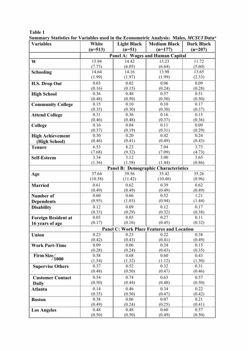
Table 1 Summary Statistics for Variables used in the Econometric Analysis: Males, MCSUI Data* Variables White

(n=513) Light Black

(n=51) Medium Black

(n=177) Dark Black

(n=207) Panel A: Wages and Human Capital

W 15.94 (7.73)

14.42 (6.05)

13.23 (6.64)

11.72 (5.60)

Schooling

14.64 (1.99)

14.16 (1.97)

13.98 (1.99)

13.65 (2.33)

H.S. Drop Out 0.03 (0.16)

0.02 (0.15)

0.06 (0.24)

0.09 (0.28)

High School 0.36 (0.48)

0.48 (0.50)

0.57 (0.50)

0.51 (0.50)

Community College 0.15 (0.35)

0.10 (0.30)

0.10 (0.30)

0.17 (0.37)

Attend College 0.31 (0.46)

0.36 (0.48)

0.16 (0.37)

0.15 (0.36)

College 0.16 (0.37)

0.04 (0.19)

0.11 (0.31)

0.09 (0.29)

High Achievement (High School)

0.30 (0.46)

0.20 (0.41)

0.42 (0.49)

0.24 (0.43)

Tenure 6.53 (7.68)

8.23 (9.32)

7.04 (7.09)

3.73 (4.73)

Self-Esteem 3.34 (1.36)

3.12 (1.58)

3.00 (1.44)

3.65 (0.86)

Panel B: Demographic Characteristics Age

37.64 (10.58)

39.56 (11.42)

35.42 (10.48)

35.26 (8.96)

Married 0.61 (0.49)

0.62 (0.49)

0.39 (0.49)

0.62 (0.49)

Number of Dependents

0.60 (0.95)

0.66 (1.03)

0.52 (0.94)

1.21 (1.44)

Disability 0.12 (0.33)

0.09 (0.29)

0.12 (0.32)

0.17 (0.38)

Foreign Resident at 16 years of age

0.03 (0.17)

0.03 (0.16)

0.27 (0.45)

0.11 (0.32)

Panel C: Work Place Features and Location Union 0.23

(0.42) 0.23

(0.43) 0.22

(0.41) 0.38

(0.49) Work Part-Time 0.09

(0.28) 0.06

(0.24) 0.24

(0.43) 0.15

(0.35)

1000Size Firm 0.58

(1.54) 0.68

(1.32) 0.60

(1.12) 0.43

(1.30) Supervise Others

0.37 (0.48)

0.52 (0.50)

0.32 (0.47)

0.31 (0.46)

Customer Contact Daily

0.54 (0.50)

0.74 (0.44)

0.63 (0.48)

0.57 (0.50)

Atlanta 0.14 (0.35)

0.46 (0.50)

0.34 (0.47)

0.22 (0.42)

Boston 0.38 (0.49)

0.06 (0.24)

0.07 (0.25)

0.21 (0.41)

Los Angeles 0.48 (0.50)

0.48 (0.50)

0.60 (0.49)

0.57 (0.50)

2

Table 1 (continued) Summary Statistics for Variables used in the Econometric Analysis: Males* Variables White

(n=513 Light Black

(n=51) Medium Black

(n=177) Dark Black

(n=207) Panel D: PreMarket Factors Mother High School Graduate

0.77 (.42)

0.63 (.49)

0.69 (.46)

0.57 (.50)

Father High School Graduate

0.72 (.45)

0.42 (.50)

0.53 (.50)

0.49 (.50)

Both Parents Raised

0.82 (0.38)

0.58 (0.50)

0.71 (0.46)

0.65 (0.48)

Welfare as a Youth

0.06 (0.24)

0.15 (0.36)

0.15 (0.36)

0.20 (0.40)

Public Housing

0.00 (.06)

0.03 (.16)

0.04 (.20)

0.04 (.20)

Religion Attendance

0.28 (0.45)

0.54 (0.50)

0.71 (0.46)

0.44 (0.50)

Jail as a Youth

0.14 (0.35)

0.19 (0.40)

0.09 (0.28)

0.15 (0.35)

Panel E: Current Neighborhood Characteristics Good Schools

0.56 (0.50)

0.50 (0.50)

0.41 (0.49)

0.38 (0.49)

Good Police

0.77 (.42)

0.49 (.50)

0.43 (.50)

0.55 (.50)

Low Crime

0.08 (0.28)

0.16 (0.37)

0.13 (0.33)

0.19 (0.39)

Panel F: Occupation of Employment Manager or Professional

0.42 (.49)

0.32 (.47)

0.19 (.39)

0.14 (.34)

Craft 0.24 (0.43)

0.16 (0.37)

0.40 (0.49)

0.29 (.45)

Services 0.10 (0.29)

0.31 (0.47)

0.18 (0.38)

0.33 (0.47)

Production 0.12 (0.33)

0.07 (0.25)

0.08 (0.27)

0.07 (0.24)

Laborers 0.12 (0.31)

0.14 (0.35)

0.15 (0.34)

0.16 (0.36)

Government 0.20 (0.40)

0.25 (0.44)

0.19 (0.39)

0.17 (0.37)

* Data Source: Multi City Survey of Urban Inequality (MCSUI). Weighted means are reported, with their standard errors in parentheses, for the sub-sample used to estimate Model 3 and Model 4.

Table 2 The Impact of Race and Skin Tone on Wages for Males: Summary Table* Data Source: Multi City Survey of Urban Inequality

Dependent Variable: ln wage rate Panel A: Bi-Variate Race (One-Drop) Model

(Race Indicator Approach) Variables Model 1

(n=968) Model 2 (n=960)

Model 3 (n=948)

Model 4 (n=948)

Model 5 (n=921)

Black -0.262*** (0.033)

-0.142*** (0.028)

-0.153*** (0.028)

-0.098*** (0.030)

-0.119*** (0.029)

F Statistic for the Equation 62.95*** [0.000]

38.92*** [0.000]

35.09*** [0.000]

23.15*** [0.000]

29.70*** [0.000]

Adjusted R Squared .06 .39 .41 .43 .43 Panel B: Skin Shade (Rainbow) Model

(Skin Shade Indicator Approach) Variables Model 1

(n=968) Model 2 (n=960)

Model 3 (n=948)

Model 4 (n=948)

Model 5 (n=921)

Light Black -0.134* (0.075)

-0.068 (0.061)

-0.076 (0.060)

-0.032 (0.061)

-0.035 (0.060)

Medium Black -0.246*** (0.044)

-0.151*** (0.037)

-0.165*** (0.037)

-0.111*** (0.039)

-0.152*** (0.037)

Dark Black -0.305*** (0.041)

-0.154*** (0.036)

-0.163*** (0.036)

-0.106*** (0.037)

-0.111*** (0.036)

H0: Light Black + Medium Black + Dark Black= 0

-38.23*** [0.000]

-15.97*** [0.000]

-19.09*** [0.000]

-6.35** [0.012]

-10.12** [0.002]

H0: Dark Black– Light Black= 0

-4.58** [0.033]

-1.70 [0.192]

-1.77 [0.183]

-1.34 [0.247]

-1.38 [0.240]

H0: Medium Black– Light Black= 0

-1.91 [0.167]

-1.56 [0.213]

-1.86 [0.173]

-1.54 [0.216]

-3.29* [0.070]

H0: Dark Black– Medium Black= 0

-1.28 [0.259]

-0.01 [0.937]

0.00 [0.956]

0.02 [0.901]

0.92 [0.339]

F Statistic for the Equation 22.66*** [0.000]

34.69*** [0.000]

31.85*** [0.000]

21.83*** [0.000]

27.59*** [0.000]

Adjusted R Squared .06 .39 .41 .43 .43 Controls for:

Human Capital yes yes yes yes Demographics yes yes yes yes Work Place Characteristics yes yes yes Family and Neighborhood yes Occupation yes

*Notes: Coefficient estimates using OLS are reported and standard errors are shown in parentheses (rounded to .001). Variables for each set of controls are described in Appendix Table 3. F-statistics, and their associated p-values shown in square brackets, are reported for tests of differences in the wage return for dark skinned and light skinned blacks. *** Statistically significant at the 99% level, 95% level, and 90% level identified by ***, **, and * respectively.

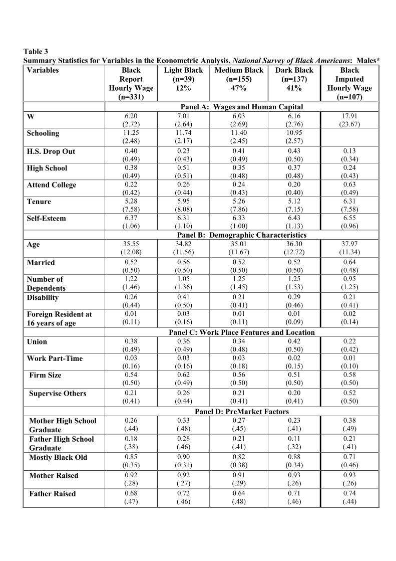
Table 3 Summary Statistics for Variables in the Econometric Analysis, National Survey of Black Americans: Males* Variables Black

Report Hourly Wage

(n=331)

Light Black (n=39) 12%

Medium Black (n=155)

47%

Dark Black (n=137)

41%

Black Imputed

Hourly Wage (n=107)

Panel A: Wages and Human Capital W 6.20

(2.72) 7.01

(2.64) 6.03

(2.69) 6.16

(2.76) 17.91

(23.67) Schooling

11.25 (2.48)

11.74 (2.17)

11.40 (2.45)

10.95 (2.57)

H.S. Drop Out 0.40 (0.49)

0.23 (0.43)

0.41 (0.49)

0.43 (0.50)

0.13 (0.34)

High School 0.38 (0.49)

0.51 (0.51)

0.35 (0.48)

0.37 (0.48)

0.24 (0.43)

Attend College 0.22 (0.42)

0.26 (0.44)

0.24 (0.43)

0.20 (0.40)

0.63 (0.49)

Tenure 5.28 (7.58)

5.95 (8.08)

5.26 (7.86)

5.12 (7.15)

6.31 (7.58)

Self-Esteem 6.37 (1.06)

6.31 (1.10)

6.33 (1.00)

6.43 (1.13)

6.55 (0.96)

Panel B: Demographic Characteristics Age

35.55 (12.08)

34.82 (11.56)

35.01 (11.67)

36.30 (12.72)

37.97 (11.34)

Married 0.52 (0.50)

0.56 (0.50)

0.52 (0.50)

0.52 (0.50)

0.64 (0.48)

Number of Dependents

1.22 (1.46)

1.05 (1.36)

1.25 (1.45)

1.25 (1.53)

0.95 (1.25)

Disability 0.26 (0.44)

0.41 (0.50)

0.21 (0.41)

0.29 (0.46)

0.21 (0.41)

Foreign Resident at 16 years of age

0.01 (0.11)

0.03 (0.16)

0.01 (0.11)

0.01 (0.09)

0.02 (0.14)

Panel C: Work Place Features and Location Union 0.38

(0.49) 0.36

(0.49) 0.34

(0.48) 0.42

(0.50) 0.22

(0.42) Work Part-Time 0.03

(0.16) 0.03

(0.16) 0.03

(0.18) 0.02

(0.15) 0.01

(0.10) Firm Size

0.54 (0.50)

0.62 (0.49)

0.56 (0.50)

0.51 (0.50)

0.58 (0.50)

Supervise Others

0.21 (0.41)

0.26 (0.44)

0.21 (0.41)

0.20 (0.41)

0.52 (0.50)

Panel D: PreMarket Factors Mother High School Graduate

0.26 (.44)

0.33 (.48)

0.27 (.45)

0.23 (.41)

0.38 (.49)

Father High School Graduate

0.18 (.38)

0.28 (.46)

0.21 (.41)

0.11 (.32)

0.21 (.41)

Mostly Black Old

0.85 (0.35)

0.90 (0.31)

0.82 (0.38)

0.88 (0.34)

0.71 (0.46)

Mother Raised

0.92 (.28)

0.92 (.27)

0.91 (.29)

0.93 (.26)

0.93 (.26)

Father Raised

0.68 (.47)

0.72 (.46)

0.64 (.48)

0.71 (.46)

0.74 (.44)

5

Table 3 (continued) Variables Black

Report Hourly Wage

(n=331)

Light Black (n=39) 12%

Medium Black (n=155)

47%

Dark Black (n=137)

41%

Black Imputed Hourly Wage

(n=107)

Panel D: PreMarket Factors (continued) Step Father

0.05 (0.22)

0.00 (0.00)

0.05 (0.22)

0.07 (0.25)

0.01 (0.10)

Grand Mother

0.19 (.40)

0.15 (.37)

0.21 (.41)

0.19 (.39)

0.25 (.44)

Grand Father

0.08 (.28)

0.08 (.27)

0.10 (.31)

0.07 (.25)

0.10 (.31)

Sisters

1.40 (1.91)

1.51 (1.62)

1.20 (1.91)

1.57 (1.98)

1.21 (1.78)

Brothers

1.51 (2.03)

1.79 (1.92)

1.30 (1.89)

1.65 (2.22)

1.43 (2.22)

Religion Important

0.90 (0.30)

0.90 (0.31)

0.89 (0.31)

0.91 (0.29)

0.92 (0.28)

Large City

0.37 (0.48)

0.41 (0.50)

0.36 (0.48)

0.35 (0.48)

0.41 (0.49)

Small City

0.17 (0.38)

0.08 (0.27)

0.19 (0.39)

0.17 (0.38)

0.17 (0.38)

Small Town

0.14 (0.35)

0.10 (0.31)

0.16 (0.36)

0.14 (0.35)

0.17 (0.38)

Suburb

0.04 (0.19)

0.05 (0.22)

0.06 (0.24)

0.01 (0.09)

0.06 (0.23)

Rural Area

0.27 (0.45)

0.31 (0.47)

0.23 (0.42)

0.32 (0.47)

0.17 (0.38)

Southern Youth

0.64 (0.48)

0.54 (0.51)

0.64 (0.48)

0.68 (0.47)

0.57 (0.50)

Panel E: Current Neighborhood Characteristics South

0.56 (0.50)

0.51 (0.51)

0.60 (0.49)

0.51 (0.50)

0.50 (0.50)

Rural

0.23 (0.42)

0.18 (0.39)

0.19 (0.40)

0.29 (0.46)

0.12 (0.33)

Mostly Black Current

0.76 (0.43)

0.82 (0.39)

0.74 (0.44)

0.77 (0.42)

0.58 (0.50)

Good Police

0.69 (0.46)

0.64 (0.49)

0.70 (0.46)

0.68 (0.47)

0.65 (0.48)

Good Schools

0.70 (.46)

0.62 (.49)

0.71 (.46)

0.72 (.45)

0.61 (.49)

Low Crime

0.68 (0.47)

0.64 (0.49)

0.68 (0.47)

0.71 (0.46)

0.75 (0.44)

Low Drugs

0.50 (.50)

0.41 (.50)

0.52 (.50)

0.51 (.50)

0.53 (.50)

Neighborhood Groups

0.37 (0.48)

0.36 (0.49)

0.34 (0.48)

0.39 (0.49)

0.37 (0.49)

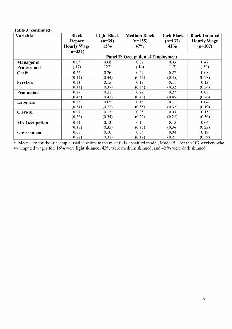
6

Table 3 (continued) Variables Black

Report Hourly Wage

(n=331)

Light Black (n=39) 12%

Medium Black (n=155)

47%

Dark Black (n=137)

41%

Black Imputed Hourly Wage

(n=107)

Panel F: Occupation of Employment Manager or Professional

0.03 (.17)

0.08 (.27)

0.02 (.14)

0.03 (.17)

0.47 (.50)

Craft 0.22 (0.41)

0.26 (0.44)

0.22 (0.41)

0.27 (0.45)

0.08 (0.28)

Services 0.13 (0.33)

0.15 (0.37)

0.13 (0.34)

0.11 (0.32)

0.13 (0.34)

Production 0.27 (0.45)

0.21 (0.41)

0.29 (0.46)

0.27 (0.45)

0.07 (0.26)

Laborers 0.13 (0.34)

0.05 (0.22)

0.18 (0.38)

0.11 (0.32)

0.04 (0.19)

Clerical

0.07 (0.26)

0.13 (0.34)

0.08 (0.27)

0.05 (0.22)

0.15 (0.36)

Mis Occupation 0.14 (0.35)

0.13 (0.35)

0.14 (0.35)

0.15 (0.36)

0.06 (0.23)

Government 0.05 (0.22)

0.10 (0.31)

0.04 (0.19)

0.04 (0.21)

0.19 (0.39)

* Means are for the subsample used to estimate the most fully specified model, Model 5. For the 107 workers who we imputed wages for; 16% were light skinned, 42% were medium skinned, and 42 % were dark skinned.

Table 4 The Impact of Skin Tone on Wages for Black Males: Summary Table*

Data Source: National Survey of Black Americans Dependent Variable: ln wage rate

Skin Shade (Rainbow) Model (Skin Shade Indicator Approach)

Variables Model 1 (n=347)

Model 2 (n=331)

Model 3 (n=331)

Model 4 (n=331)

Model 5 (n=331)

Light Black 0.183** (0.077)

.107* (0.065)

0.107* (0.061)

0.126** (0.062)

0.107* (0.059)

Dark Black

0.011 (0.050)

0.021 (0.042)

0.0123 (0.034)

0.030 (0.042)

-0.003 (0.038)

H0: Light Black – Dark Black = 0

4.91** [0.028]

1.73 [0.190]

2.37 [0.125]

2.23 [0.136]

3.50* [0.062]

F Statistic for the Equation 2.98** [0.027]

13.76*** [0.000]

14.87*** [0.000]

7.27*** [0.000]

13.60*** [0.000]

Adjusted R Squared

.01

.35

.43

.43

.49

Controls for: Human Capital yes yes yes yes Demographics yes yes yes yes Work Place Characteristics yes yes yes Family and Neighborhood yes Occupation yes

*Notes: Coefficient estimates using OLS are reported and standard errors are shown in parentheses (rounded to .001). Variables for each set of controls are described in Appendix Table 3. F-statistics, and their associated p-values shown in square brackets, are reported for tests of differences in the wage return for dark skinned and light skinned blacks. *** Statistically significant at the 99% level, 95% level, and 90% level identified by ***, **, and * respectively.

Table 5A Inter-Racial Wage Decompositions: Characteristic and Treatment Wage Effects for White Workers Relative to Black Workers in Alternative Skin Shade Groups, MCSUI Data * Characteristic Effect (%) Treatment Effect (%) Inter-Racial Group Comparison (White: Other Group)

Other Group % of White

Group Wage

Characteristic Advantage

White

Characteristic Advantage

White

Treatment Advantage

White

Treatment Disadvantage Other Group

Panel A: Model 3

White: Black 78.60 10.38 11.99 11.98 14.03 White: Dark Black 77.13 12.14 11.85 13.73 13.92 White: Medium Black 78.51 10.85 10.62 13.15 13.56 White: Light Black 96.73 -2.52 -1.36 4.59 5.99 Panel B: Model 4

White: Black 79.21 14.34 19.15 5.62 8.14 White: Dark Black 75.98 13.44 21.64 7.57 13.92 White: Medium Black 77.42 14.74 21.27 6.11 10.13 White: Light Black 98.63 3.31 13.01 -11.46 -1.97

Panel C: Model 5

White: Black

79.09 13.60 13.52 10.22 9.24

White: Dark Black 77.28 15.57 16.62 9.87 9.25 White: Medium Black 80.26 13.80 10.09 11.64 7.40 White: Light Black 96.47 1.50 -3.14 6.56 2.11

Data Source: Multi City Survey of Urban Inequality (MCSUI). Subsample sizes; white (n = 513). dark black (n = 207), medium black (n = 177), and light black (n = 51). i

jwˆˆ = Predicted wage using the estimated coefficients

for the thi group and the levels of the characteristics of the thj group. The predicted wage for the reference

group R is RRw ˆˆ . Comparing white workers (W) who are an in-group with dark black workers (D), an out-group,

the: ( ) ( )

−

−=WW

WW

DW

w

wwAdvantageTreatment ˆ

ˆˆ

ˆ

ˆˆ1 , ( )

,ˆ

ˆˆ ˆ

ˆˆ

−

=DD

DD

WD

w

wwgeDisadvantaTreatment

( ) ( ),

ˆ

ˆˆ1 ˆ

ˆˆ

−

−=WW

WW

WD

w

wwAdvantagesticsCharacteri and

( ).

ˆˆˆ

ˆ

ˆˆ

−

=DD

DD

DW

www

geDisadvantasticsCharacteri

Table 5B Intra-Racial Wage Decompositions: Treatment and Characteristics Wage Effects for Black Workers as a Group Relative to Black Workers in Alternative Skin Shade Groups, MCSUI Data * Characteristic Effect (%) Treatment Effect (%) Intra-Racial Group Comparison (Black: Other Group)

Other Group % of Black

Group Wage

Characteristic Advantage

Black

Characteristic Disadvantage Other Group

Treatment Advantage

Black

Treatment Disadvantage Other Group

Panel A: Model 3

Black: Dark Black 98.13 1.90 0.28 1.59 -0.03 Black: Medium Black 99.89 -0.11 -2.18 2.29 0.23 Black: Light Black 123.07 -10.39 -17.33 -1.74 -10.30 Panel B: Model 4

Black: Dark Black 95.93 4.10 3.54 0.68 -0.03 Black: Medium Black 97.74 -0.49 -0.87 3.11 2.81 Black: Light Black 124.51 -9.92 -10.47 -11.48 -11.72

Panel C: Model 5

Black: Dark Black 97.72 3.72 2.79 -0.45 -1.47 Black: Medium Black 101.49 -2.50 -3.96 2.54 1.00 Black: Light Black 121.98 -7.95 -17.44 -0.71 -11.50

* Data Source: Multi City Survey of Urban Inequality (MCSUI). Subsample sizes; white (n = 513). dark black (n = 207), medium black (n = 177), and light black (n = 51). i

jwˆˆ = Predicted wage using the estimated

coefficients for the thi group and the levels of the characteristics of the thj group. The predicted wage for the

reference group R is RRw ˆˆ . Comparing white workers (W) who are an in-group with dark black workers (D), an

out-group, the: ( ) ( )

−

−=WW

WW

DW

w

wwAdvantageTreatment ˆ

ˆˆ

ˆ

ˆˆ1 , ( )

,ˆ

ˆˆ ˆ

ˆˆ

−

=DD

DD

WD

w

wwgeDisadvantaTreatment

( ) ( ),

ˆ

ˆˆ1 ˆ

ˆˆ

−

−=WW

WW

WD

w

wwAdvantagesticsCharacteri and

( ).

ˆˆˆ

ˆ

ˆˆ

−

=DD

DD

DW

www

geDisadvantasticsCharacteri

Table 5C Intra-Racial Wage Decompositions: Treatment and Characteristics Wage Effects for Black Workers as a Group Relative to Black Workers in Alternative Skin Shade Groups, NSBA Data * Characteristic Effect (%) Treatment Effect (%) Intra-Racial Group Comparison (Black: Other Group)

Other Group % of White

Group Black

Characteristic Advantage

Black

Characteristic Disadvantage Other Group

Treatment Advantage

Black

Treatment Disadvantage Other Group

Panel A: Model 3

Black: Dark Black

99.20 0.28 0.82 -0.01 0.53

Black: Medium Black 97.13 1.22 1.64 1.27 1.69 Black: Light Black

115.49 -6.05 0.64 -16.23 -8.17

Panel B: Model 4

Black: Dark Black 99.20 1.04 0.47 0.34 -0.24 Black: Medium Black 97.13 0.48 0.78 2.11 2.46 Black: Light Black** 115.49 N/A N/A N/A N/A

Panel C: Model 5

Black: Dark Black 99.20 -0.58 0.24 0.56 1.39 Black: Medium Black 97.13 1.87 2.63 0.32 1.03 Black: Light Black 115.49 -5.64 2.88 -18.81 -8.53

* Data Source: Multi City Survey of Urban Inequality (MCSUI). Subsample sizes; white (n = 513). dark black (n = 207), medium black (n = 177), and light black (n = 51). i

jwˆˆ = Predicted wage using the estimated

coefficients for the thi group and the levels of the characteristics of the thj group. The predicted wage for the

reference group R is RRw ˆˆ . Comparing white workers (W) who are an in-group with dark black workers (D), an

out-group, the: ( ) ( )

−

−=WW

WW

DW

w

wwAdvantageTreatment ˆ

ˆˆ

ˆ

ˆˆ1 , ( )

,ˆ

ˆˆ ˆ

ˆˆ

−

=DD

DD

WD

w

wwgeDisadvantaTreatment

( ) ( ),

ˆ

ˆˆ1 ˆ

ˆˆ

−

−=WW

WW

WD

w

wwAdvantagesticsCharacteri and

( ).

ˆˆˆ

ˆ

ˆˆ

−

=DD

DD

DW

www

geDisadvantasticsCharacteri

**Due to missing observations all parameters of the subsample of light skin Blacks could not be estimated for Model 4.

Appendix Table 1 Sample Creation: Multi City Survey of Urban Inequality (MCSUI) Data.* MCSUI total sample

8916

Source of Data Deletion

Deletions

Remaining

Missing /invalid ethnicity code

133 8783

Detroit

1418 7365

Females

4367 2998

Non-blacks & non-whites

1224 1774

Older than 65

276 1498

Self-employed

176 1322

Retired or out of labor force for past five years

167 1155

Refused to provide, don’t know, or missing earnings data

151 1004

Earn more than 100,000 per year

6 998

Refused to provide, don’t know, or missing hours worked per week

3 995

Hourly wage greater than 100 or less than 2

27 968

Missing/invalid on any human capital (including tenure) variable

8 960

Missing/invalid on any work place setting variable

12 948

Missing/invalid on any occupation code

37

921

* Data Source: Multi City Survey of Urban Inequality (MCSUI).

Appendix Table 2 Definition of Variables: Data Source, Multi City Survey of Urban Inequality (MCSUI) Variables Variable Definitions

Variables Variable Definitions

W Respondents hourly wage Foreign Resident at 16 years of age

1 if respondent was primarily a foreign resident before 16 years of age, 0 otherwise

White 1 if respondent is White, 0 otherwise

Los Angeles 1 if respondent resides in Los Angeles, 0 otherwise

Light Black 1 if respondent is Black and has light skin-tone, 0 otherwise

Atlanta 1 if respondent resides in Atlanta, 0 otherwise

Medium Black 1 if respondent is Black and has medium skin-tone, 0 otherwise

Boston 1 if respondent resides in Boston, 0 otherwise

Dark Black 1 if respondent is Black and has dark skin-tone, 0 otherwise

Union 1 if respondent is a union member, 0 otherwise

Age Respondents age

Work Part-Time 1 if respondent works part-time, 0 otherwise

Schooling

Years of schooling completed Firm Size Number of workers at respondents firm per 1,000 workers

Tenure Number of years employed by current employer

Mother Education

1 if respondent’s mother completed at least 12 years of formal schooling, 0 otherwise

H.S. Drop Out 1 if respondent failed to complete High School, 0 otherwise

Father Education

1 if respondent’s father completed at least 12 years of formal schooling, 0 otherwise

High School 1 if respondents highest level of schooling is completion of High School, 0 otherwise

Both Parents Raised

1 if lived with mother and father to age 16, 0 otherwise

Community College

1 if respondents highest level of schooling is completion of Community College, 0 otherwise

Mother Raised 1 if lived with mother to age 16, 0 otherwise

Attend College 1 if respondents highest level of schooling was attending College, 0 otherwise

Father Raised 1 if lived with father to age 16, 0 otherwise

College 1 if respondent completed College School, 0 otherwise

Grand Parent Raised

1 if lived with grand parent(s), not parents, to age 16, 0 otherwise

High Achievement 1 if respondent average High School grade is B or better, 0 otherwise

Other Raised 1 if lived with someone other than parent(s) or grand parent(s), to age 16, 0 otherwise

Self-Esteem Rosenberg Self-esteem Score. Scores range in ascending order from 0 to 4,

Religion Attendance

1 if respondent attended church at least once a month growing up, 0 otherwise

Married 1 if respondent is married or living with a partner, 0 otherwise

Welfare as a Youth

1 if respondent’s family was on welfare at some point up to age 16, 0 otherwise

Number of Dependents

Number of dependents in the household

Jail as a Youth 1 if respondent has ever been incarcerated or attended reform school, 0 otherwise

Disability 1 if respondent has a work limiting health condition, 0 otherwise

Public Housing 1 if respondent currently lives in public housing, 0 otherwise

3

Appendix Table 2 (continued) Definition of Variables: Data Source, Multi City Survey of Urban Inequality (MCSUI) Variables Variable Definitions

Variables Variable Definitions

Good Police 1 if respondent believes police services in current neighborhood are good, 0 otherwise

White Coworkers

1 if respondents coworkers are predominantly White, 0 otherwise

Good Schools 1 if respondent believes public schools in current neighborhood are good, 0 otherwise

Black Coworkers

1 if respondents coworkers are predominantly Black, 0 otherwise

Low Crime 1 if respondent believes level of crime is low in the current neighborhood, 0 otherwise

Hispanic Coworkers

1 if respondents coworkers are predominantly Hispanic, 0 otherwise

Supervise Others

1 if respondent supervises other employees, 0 otherwise

Asian Coworkers

1 if respondents coworkers are predominantly Asian, 0 otherwise

Customer Contact Daily

1 if respondent talks to customers daily at work, 0 otherwise

Other Coworkers

1 if respondents coworkers are not predominantly; White, Black, Hispanic, or Asian, 0 otherwise

Manager or Professional

1 if respondent is in a managerial or professional occupation, 0 otherwise

Supervisor White

1 if respondents supervisor is White, 0 otherwise

Production 1 if respondent is in a precision production, craft or repair occupation, 0 otherwise

Supervisor Black

1 if respondents supervisor is Black, 0 otherwise

Services 1 if respondent is in a service occupation, 0 otherwise

Supervisor Hispanic

1 if respondents supervisor is Hispanic, 0 otherwise

Craft 1 if respondent is in a craft occupation, 0 otherwise

Supervisor Asian

1 if respondents supervisor is Asian, 0 otherwise

Laborers 1 if respondent is in a laborer occupation, 0 otherwise

Supervisor Other

1 if respondents supervisor is not; White, Black, Hispanic, or Asian, 0 otherwise

Government 1 if respondent is in a public employee, 0 otherwise

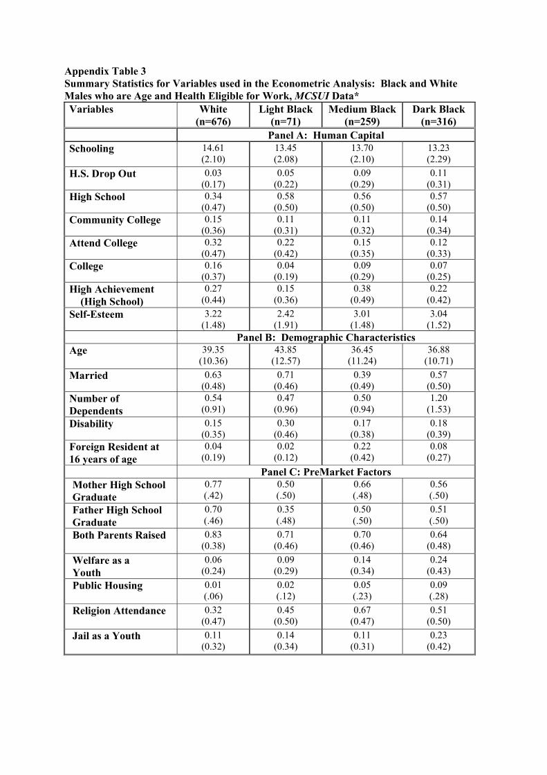
Appendix Table 3 Summary Statistics for Variables used in the Econometric Analysis: Black and White Males who are Age and Health Eligible for Work, MCSUI Data* Variables White

(n=676) Light Black

(n=71) Medium Black

(n=259) Dark Black

(n=316) Panel A: Human Capital

Schooling

14.61 (2.10)

13.45 (2.08)

13.70 (2.10)

13.23 (2.29)

H.S. Drop Out 0.03 (0.17)

0.05 (0.22)

0.09 (0.29)

0.11 (0.31)

High School 0.34 (0.47)

0.58 (0.50)

0.56 (0.50)

0.57 (0.50)

Community College 0.15 (0.36)

0.11 (0.31)

0.11 (0.32)

0.14 (0.34)

Attend College 0.32 (0.47)

0.22 (0.42)

0.15 (0.35)

0.12 (0.33)

College 0.16 (0.37)

0.04 (0.19)

0.09 (0.29)

0.07 (0.25)

High Achievement (High School)

0.27 (0.44)

0.15 (0.36)

0.38 (0.49)

0.22 (0.42)

Self-Esteem 3.22 (1.48)

2.42 (1.91)

3.01 (1.48)

3.04 (1.52)

Panel B: Demographic Characteristics Age

39.35 (10.36)

43.85 (12.57)

36.45 (11.24)

36.88 (10.71)

Married 0.63 (0.48)

0.71 (0.46)

0.39 (0.49)

0.57 (0.50)

Number of Dependents

0.54 (0.91)

0.47 (0.96)

0.50 (0.94)

1.20 (1.53)

Disability 0.15 (0.35)

0.30 (0.46)

0.17 (0.38)

0.18 (0.39)

Foreign Resident at 16 years of age

0.04 (0.19)

0.02 (0.12)

0.22 (0.42)

0.08 (0.27)

Panel C: PreMarket Factors Mother High School Graduate

0.77 (.42)

0.50 (.50)

0.66 (.48)

0.56 (.50)

Father High School Graduate

0.70 (.46)

0.35 (.48)

0.50 (.50)

0.51 (.50)

Both Parents Raised

0.83 (0.38)

0.71 (0.46)

0.70 (0.46)

0.64 (0.48)

Welfare as a Youth

0.06 (0.24)

0.09 (0.29)

0.14 (0.34)

0.24 (0.43)

Public Housing

0.01 (.06)

0.02 (.12)

0.05 (.23)

0.09 (.28)

Religion Attendance

0.32 (0.47)

0.45 (0.50)

0.67 (0.47)

0.51 (0.50)

Jail as a Youth

0.11 (0.32)

0.14 (0.34)

0.11 (0.31)

0.23 (0.42)

5

Appendix Table 3 Summary Statistics for Variables used in the Econometric Analysis: Males* Variables White

(n=676) Light Black

(n=71) Medium Black

(n=259) Dark Black

(n=316) Panel D: Location

Atlanta 0.18 (0.38)

0.35 (0.48)

0.39 (0.49)

0.22 (0.41)

Boston 0.36 (0.48)

0.05 (0.22)

0.06 (0.24)

0.18 (0.38)

Los Angeles 0.45 (0.49)

0.60 (0.49)

0.55 (0.50)

0.61 (0.49)

Panel E: Current Neighborhood Characteristics Good Schools

0.59 (0.49)

0.42 (0.50)

0.46 (0.50)

0.42 (0.50)

Good Police

0.79 (.41)

0.42 (.50)

0.44 (.50)

0.58 (.49)

Low Crime

0.08 (0.27)

0.12 (0.33)

0.14 (0.34)

0.16 (0.36)

* Data Source: Multi City Survey of Urban Inequality (MCSUI). Weighted means are reported with their standard errors in parentheses.

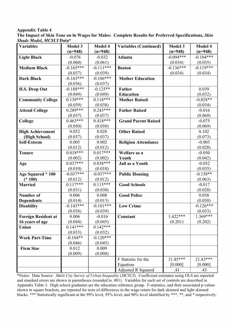
Appendix Table 4 The Impact of Skin Tone on ln Wages for Males: Complete Results for Preferred Specifications, Skin Shade Model, MCSUI Data* Variables Model 3

(n=948) Model 4 (n=948)

Variables (Continued) Model 3 (n=948)

Model 4 (n=948)

Light Black -0.076 (0.060)

-0.032 (0.061)

Atlanta -0.094*** (0.034)

-0.104*** (0.035)

Medium Black

-0.165*** (0.037)

-0.111*** (0.039)

Boston -0.136*** (0.034)

-0.119*** (0.034)

Dark Black

-0.163*** (0.036)

-0.106*** (0.037)

Mother Education

H.S. Drop Out -0.188*** (0.049)

-0.125** (0.049)

Father Education

0.039 (0.032)

Community College 0.139*** (0.039)

0.118*** (0.038)

Mother Raised -0.028** (0.034)

Attend College 0.289*** (0.037)

0.243*** (0.037)

Father Raised -0.016 (0.069)

College 0.463*** (0.050)

0.418*** (0.050)

Grand Parent Raised -0.075 (0.069)

High Achievement (High School)

0.052 (0.037)

0.028 (0.037)

Other Raised 0.102 (0.073)

Self-Esteem 0.005 (0.012)

0.002 (0.012)

Religion Attendance -0.003 (0.028)

Tenure 0.018*** (0.002)

0.017*** (0.002)

Welfare as a Youth

-0.050 (0.042)

Age

0.037*** (0.010)

0.038*** (0.010)

Jail as a Youth -0.052 (0.035)

Age Squared * 100 (* 100)

-0.037*** (0.012)

-0.037*** (0.012)

Public Housing -0.158** (0.063)

Married 0.117*** (0.031)

0.115*** (0.030)

Good Schools -0.017 (0.028)

Number of Dependents

0.006 (0.014)

0.008 (0.013)

Good Police 0.038 (0.030)

Disability -0.143*** (0.038)

-0.101*** (0.039)

Low Crime -0.126*** (0.033)

Foreign Resident at 16 years of age

0.006 (0.044)

-0.016 (0.045)

Constant 1.422*** (0.201)

1.369*** (0.202)

Union 0.141*** (0.033)

0.142*** (0.032)

Work Part-Time -0.104** (0.046)

-0.120*** (0.045)

Firm Size

0.012 (0.009)

0.009 (0.008)

F Statistic for the Equation

31.85*** [0.000]

21.83*** [0.000]

Adjusted R Squared .41 .43 *Notes: Data Source: Multi City Survey of Urban Inequality (MCSUI). Coefficient estimates using OLS are reported and standard errors are shown in parentheses (rounded to .001). Variables for each set of controls are described in Appendix Table 3. High school graduates are the education reference group. F-statistics, and their associated p-values shown in square brackets, are reported for tests of differences in the wage return for dark skinned and light skinned blacks. *** Statistically significant at the 99% level, 95% level, and 90% level identified by ***, **, and * respectively.

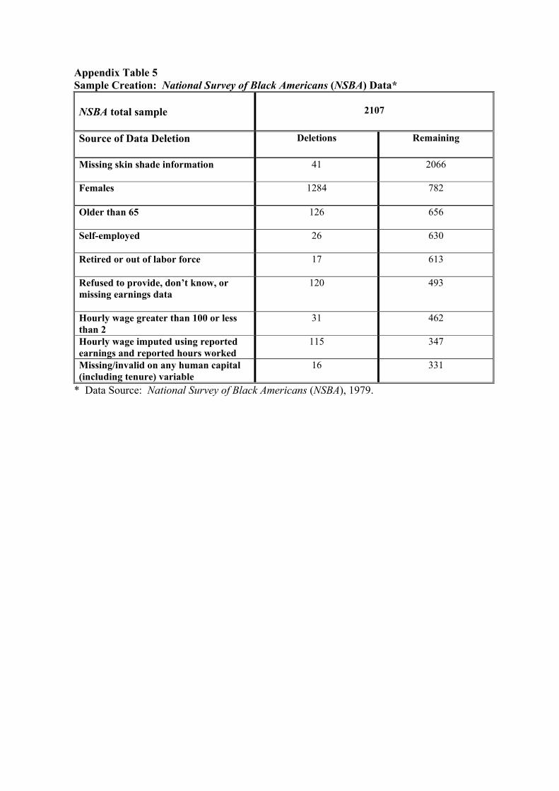
Appendix Table 5 Sample Creation: National Survey of Black Americans (NSBA) Data* NSBA total sample

2107

Source of Data Deletion

Deletions

Remaining

Missing skin shade information

41 2066

Females

1284 782

Older than 65

126 656

Self-employed

26 630

Retired or out of labor force

17 613

Refused to provide, don’t know, or missing earnings data

120 493

Hourly wage greater than 100 or less than 2

31 462

Hourly wage imputed using reported earnings and reported hours worked

115 347

Missing/invalid on any human capital (including tenure) variable

16 331

* Data Source: National Survey of Black Americans (NSBA), 1979.

Appendix Table 6 Definition of Variables: Data Source, National Survey of Black Americans (NSBA) Variables Variable Definitions

Variables Variable Definitions

W Respondents hourly wage Supervise Others

1 if respondent supervises other employees, 0 otherwise

Light Black 1 if respondent is Black and has light skin-tone, 0 otherwise

Manager or Professional

1 if respondent is in a managerial or professional occupation, 0 otherwise

Medium Black 1 if respondent is Black and has medium skin-tone, 0 otherwise

Production 1 if respondent is in a precision production, craft or repair occupation, 0 otherwise

Dark Black 1 if respondent is Black and has dark skin-tone, 0 otherwise

Services 1 if respondent is in a service occupation, 0 otherwise

Age Respondents age

Craft 1 if respondent is in a craft occupation, 0 otherwise

Schooling

Years of schooling completed Laborers 1 if respondent is in a laborer occupation, 0 otherwise

Tenure Number of years employed by current employer

Clerical 1 if respondent is in a clerical occupation, 0 otherwise

H.S. Drop Out 1 if respondent failed to complete High School, 0 otherwise

Mis Occupation 1 if respondent occupation code is missing or unreported, 0 otherwise

High School 1 if respondents highest level of schooling is completion of High School, 0 otherwise

Government 1 if respondent is in a public employee, 0 otherwise

Attend College 1 if respondents highest level of schooling was at least attending College, 0 otherwise

Mostly Black Old

1 if respondent lived in a mostly black neighborhood at 16, 0 otherwise

Self-Esteem Rosenberg Self-esteem Score. Scores range in ascending order from 0 to 7,

Mother Education

1 if respondent’s mother completed at least 12 years of formal schooling, 0 otherwise

Married 1 if respondent is married or living with a partner, 0 otherwise

Father Education

1 if respondent’s father completed at least 12 years of formal schooling, 0 otherwise

Number of Dependents

Number of dependents in the household

Mother Raised 1 if mother lived in the home when respondent was 16, 0 otherwise

Disability 1 if respondent has a work limiting health condition, 0 otherwise

Father Raised 1 if father lived in the home when respondent was 16, 0 otherwise

Foreign Resident at 16 years of age

1 if respondent was primarily a foreign resident before 16 years of age, 0 otherwise

Step Father 1 if step father lived in the home when respondent was 16, 0 otherwise

South 1 if respondent resides in a southern state in the U.S., 0 otherwise

Grand Mother

1 if grand mother lived in the home when respondent was 16, 0 otherwise

Rural 1 if respondent resides in a rural community, 0 otherwise

Grand Father 1 if grand father lived in the home when respondent was 16, 0 otherwise

Union 1 if respondent is a union member, 0 otherwise

Sisters # of sisters living in respondent’s home when respondent was 16

Work Part-Time 1 if respondent works part-time, 0 otherwise

Brothers # of brothers living in respondent’s home when respondent was 16

Firm Size Number of workers at respondents firm per 1,000 workers

Religion Important

1 if religion fairly important when growing up, 0 otherwise

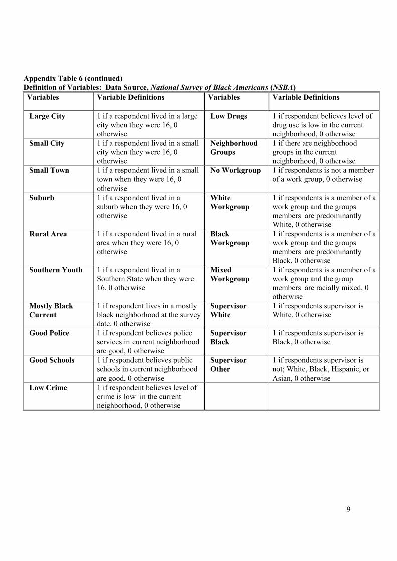
9

Appendix Table 6 (continued) Definition of Variables: Data Source, National Survey of Black Americans (NSBA) Variables Variable Definitions

Variables Variable Definitions

Large City 1 if a respondent lived in a large city when they were 16, 0 otherwise

Low Drugs 1 if respondent believes level of drug use is low in the current neighborhood, 0 otherwise

Small City 1 if a respondent lived in a small city when they were 16, 0 otherwise

Neighborhood Groups

1 if there are neighborhood groups in the current neighborhood, 0 otherwise

Small Town 1 if a respondent lived in a small town when they were 16, 0 otherwise

No Workgroup 1 if respondents is not a member of a work group, 0 otherwise

Suburb 1 if a respondent lived in a suburb when they were 16, 0 otherwise

White Workgroup

1 if respondents is a member of a work group and the groups members are predominantly White, 0 otherwise

Rural Area 1 if a respondent lived in a rural area when they were 16, 0 otherwise

Black Workgroup

1 if respondents is a member of a work group and the groups members are predominantly Black, 0 otherwise

Southern Youth 1 if a respondent lived in a Southern State when they were 16, 0 otherwise

Mixed Workgroup

1 if respondents is a member of a work group and the group members are racially mixed, 0 otherwise

Mostly Black Current

1 if respondent lives in a mostly black neighborhood at the survey date, 0 otherwise

Supervisor White

1 if respondents supervisor is White, 0 otherwise

Good Police 1 if respondent believes police services in current neighborhood are good, 0 otherwise

Supervisor Black

1 if respondents supervisor is Black, 0 otherwise

Good Schools 1 if respondent believes public schools in current neighborhood are good, 0 otherwise

Supervisor Other

1 if respondents supervisor is not; White, Black, Hispanic, or Asian, 0 otherwise

Low Crime 1 if respondent believes level of crime is low in the current neighborhood, 0 otherwise

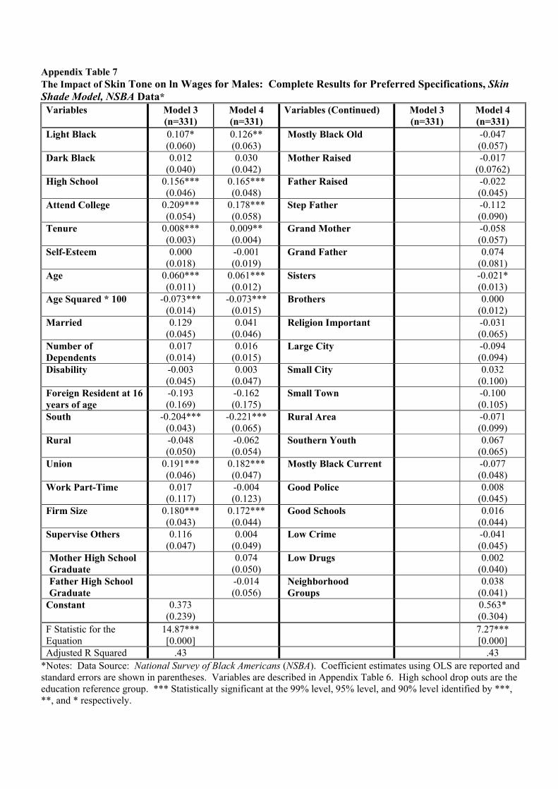
Appendix Table 7 The Impact of Skin Tone on ln Wages for Males: Complete Results for Preferred Specifications, Skin Shade Model, NSBA Data* Variables Model 3

(n=331) Model 4 (n=331)

Variables (Continued) Model 3 (n=331)

Model 4 (n=331)

Light Black 0.107* (0.060)

0.126** (0.063)

Mostly Black Old

-0.047 (0.057)

Dark Black

0.012 (0.040)

0.030 (0.042)

Mother Raised

-0.017 (0.0762)

High School

0.156*** (0.046)

0.165*** (0.048)

Father Raised

-0.022 (0.045)

Attend College 0.209*** (0.054)

0.178*** (0.058)

Step Father

-0.112 (0.090)

Tenure 0.008*** (0.003)

0.009** (0.004)

Grand Mother

-0.058 (0.057)

Self-Esteem 0.000 (0.018)

-0.001 (0.019)

Grand Father

0.074 (0.081)

Age

0.060*** (0.011)

0.061*** (0.012)

Sisters

-0.021* (0.013)

Age Squared * 100

-0.073*** (0.014)

-0.073*** (0.015)

Brothers

0.000 (0.012)

Married 0.129 (0.045)

0.041 (0.046)

Religion Important

-0.031 (0.065)

Number of Dependents

0.017 (0.014)

0.016 (0.015)

Large City

-0.094 (0.094)

Disability -0.003 (0.045)

0.003 (0.047)

Small City

0.032 (0.100)

Foreign Resident at 16 years of age

-0.193 (0.169)

-0.162 (0.175)

Small Town

-0.100 (0.105)

South -0.204*** (0.043)

-0.221*** (0.065)

Rural Area

-0.071 (0.099)

Rural -0.048 (0.050)

-0.062 (0.054)

Southern Youth

0.067 (0.065)

Union 0.191*** (0.046)

0.182*** (0.047)

Mostly Black Current -0.077 (0.048)

Work Part-Time 0.017 (0.117)

-0.004 (0.123)

Good Police

0.008 (0.045)

Firm Size 0.180*** (0.043)

0.172*** (0.044)

Good Schools

0.016 (0.044)

Supervise Others

0.116 (0.047)

0.004 (0.049)

Low Crime

-0.041 (0.045)

Mother High School Graduate

0.074 (0.050)

Low Drugs

0.002 (0.040)

Father High School Graduate

-0.014 (0.056)

Neighborhood Groups

0.038 (0.041)

Constant

0.373 (0.239)

0.563* (0.304)

F Statistic for the Equation

14.87*** [0.000]

7.27*** [0.000]

Adjusted R Squared .43 .43 *Notes: Data Source: National Survey of Black Americans (NSBA). Coefficient estimates using OLS are reported and standard errors are shown in parentheses. Variables are described in Appendix Table 6. High school drop outs are the education reference group. *** Statistically significant at the 99% level, 95% level, and 90% level identified by ***, **, and * respectively.

11