Friction in Automotive Engines - InTech - OpenFriction in Automotive Engines 3 Figure 1. Friction measurement test-rig FRIDA during build-up at the Virtual Vehicle Competence Center

Chapter 0

Friction in Automotive Engines

H. Allmaier, C. Priestner, D.E. Sander and F.M. Reich

Additional information is available at the end of the chapter

http://dx.doi.org/10.5772/51568

1. Introduction

The current situation of the automotive industry is a challenging one. On one hand, theongoing trend to more luxury cars brings more and more benefits to the customer and iscertainly also an important selling point. The same applies to the increased safety levelsmodern cars have to provide. However, both of these benefits come with a severe inherentdrawback and that is extra weight and, consequently, higher fuel consumption. On theother hand, increased fuel consumption is not only a disadvantage due to the ever risingfuel costs and the corresponding customer demand for more efficient cars. Due to thecorresponding greenhouse gas emissions it is also in the focus of the legislation in manycountries. Commonly road transport is estimated [13, 15] to cause about 75-89 % of thetotal CO2 emissions within the world’s transportation sector and for about 20% of the globalprimary energy consumption [12]. These values do not stay constant; in the time from 1990 to2005, the required energy for transportation increased by 37% [11] and further increases areexpected due to the evolving markets in the developing countries. As industrial emissionsdecrease, the rising energy demand in the transport sector is expected to be the majorproblem to achieve a significant greenhouse gas reduction [26]. Consequently, about allmajor automotive markets introduce increasingly strict emission limits like the national fueleconomy program implemented in the CAFE regulations in the US, the EURO regulation inthe European Union or the FES in China.

In particular, the European union introduced a limit for the average CO2 emissions for allcars to be available on the European market of 130 g CO2/km by 20151. Further, a long termtarget of 95 g CO2/km was specified for 2020 [6]. To put this into perspective, the averagefleet consumption in 2007 was 158 g CO2/km and it had taken already about 10 years toget down to this value from the 180 g CO2/km that were achieved in 1998. Now a largerreduction is required in less time. The required reduction of emissions brings also a directbenefit for the customer as the fuel consumption is lowered. It is estimated [11] that the

1 The limit applies to the average fleet consumption of every car manufacturer, calculated by averaging the fuelconsumption of all offered car models and weighted by the number of sold units of the specific models.

©2013 Allmaier et al., licensee InTech. This is an open access chapter distributed under the terms of theCreative Commons Attribution License (http://creativecommons.org/licenses/by/3.0),which permitsunrestricted use, distribution, and reproduction in any medium, provided the original work is properlycited.

Chapter 9

2 Will-be-set-by-IN-TECH

average car consumes every year about 169 litres of fuel only to overcome mechanical frictionin the powertrain. There exist several efficient measures to lower the emissions, notably todecrease the weight of the car itself to reduce the energy needed for acceleration, to optimizethe combustion process and, of course, to reduce all inherent power losses like the tyre rollingresistance, aerodynamic drag and mechanical losses of the powertrain (combination of engineand transmission) itself. These measures are, however, not straightforward as some havedrawbacks or are even in conflict with each other. For example, smaller cars that offer reducedweight have commonly worse aerodynamic drag as their shape is more cube-like for practicalreasons [8]. Also, a reduction in aerodynamic drag brings only a small benefit in the urbantraffic due to the low cruising speeds involved. A reduction of tyre rolling resistance is hard toachieve without reduced performance in other areas like handling and traction [10]. Weightreduction is expensive as more and more lightweight and expensive materials have to beused, some of which also require a lot of energy in the production process. In addition, it wasshown [8] that there is no positive synergy effect: the combination of several of the mentionedmeasures reduces their individual efficiency, such that their combination brings less benefitthan anticipated.

In contrast, making the powertrain more efficient yields a proportional reduction in CO2emissions [8]. For low load operating conditions of Diesel engines friction reduction is eventhe prime measure to further decrease fuel consumption [16]. While currently a lot of work isdone in the automotive industry to reduce the losses caused by the auxiliary systems like theoil or coolant pump, it was shown at hand of a specific engine that the potential for frictionreduction in the ICE itself is of comparable magnitude [16].

2. Sources of friction in ICEs

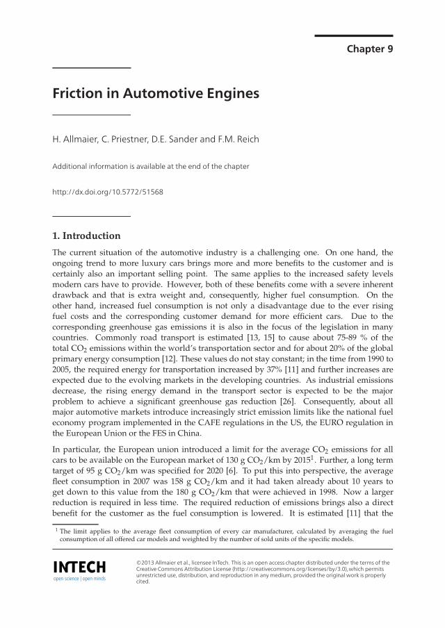
Before any efficient measures to reduce friction in engines can take place, the main frictionsources need to be known. At the Virtual Vehicle Competence Center, we use our frictiontest-rig as shown in Fig. 1 to investigate the sources of friction for a typical four cylindergasoline engine; exemplary results for this engine are shown in Fig. 2.

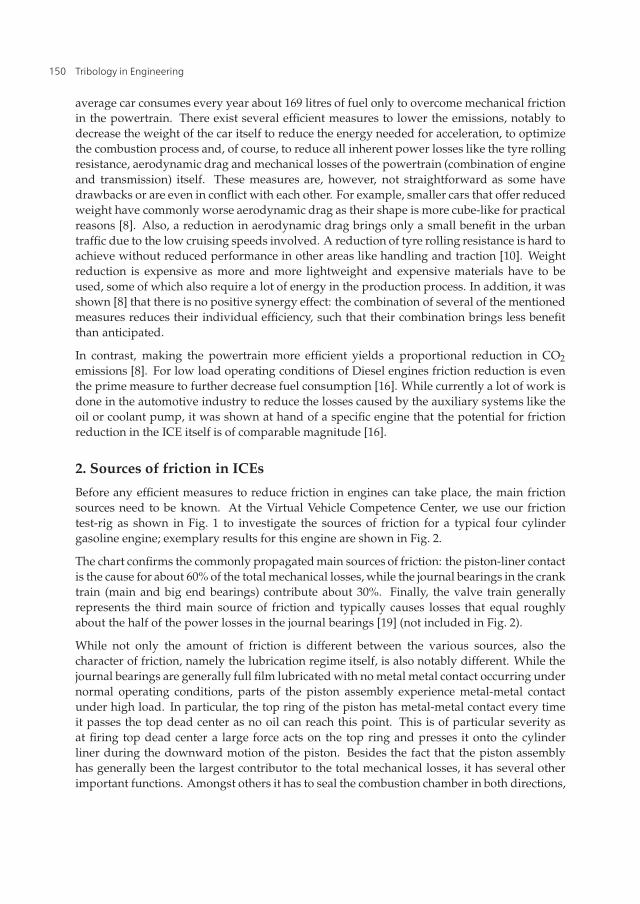
The chart confirms the commonly propagated main sources of friction: the piston-liner contactis the cause for about 60% of the total mechanical losses, while the journal bearings in the cranktrain (main and big end bearings) contribute about 30%. Finally, the valve train generallyrepresents the third main source of friction and typically causes losses that equal roughlyabout the half of the power losses in the journal bearings [19] (not included in Fig. 2).

While not only the amount of friction is different between the various sources, also thecharacter of friction, namely the lubrication regime itself, is also notably different. While thejournal bearings are generally full film lubricated with no metal metal contact occurring undernormal operating conditions, parts of the piston assembly experience metal-metal contactunder high load. In particular, the top ring of the piston has metal-metal contact every timeit passes the top dead center as no oil can reach this point. This is of particular severity asat firing top dead center a large force acts on the top ring and presses it onto the cylinderliner during the downward motion of the piston. Besides the fact that the piston assemblyhas generally been the largest contributor to the total mechanical losses, it has several otherimportant functions. Amongst others it has to seal the combustion chamber in both directions,

150 Tribology in Engineering

Friction in Automotive Engines 3

Figure 1. Friction measurement test-rig FRIDA during build-up at the Virtual Vehicle CompetenceCenter. It is shown being applied to an inline four cylinder gasoline engine with 1.8 litres totaldisplacement.

both to avoid so-called blow-by gases from entering the engine housing, as well as to controlthe amount of lubricant being left on the cylinder liner. The blow-by gases have to becontrolled as these both cause a loss in convertible energy by decreasing the available cylinderpressure as well as have a negative deteriorating impact on the lubricant properties. Theoil being left on the cylinder liner needs to be carefully controlled as well: while a certainamount of oil is necessary to provide sufficient lubrication for the piston rings, it is burnedduring combustion. Burning too much oil needs to be avoided not only for practical reasonsas it needs to be replaced (increased service demand), but also as some of its contents areproblematic for the exhaust aftertreatment systems.

Additionally, depending on operating condition unstable behaviour of the piston rings mayoccur [27] like ring flutter (rapid oscillating movement of the piston ring in its groove) orring collapse (inward forces on the ring exceed the ring tension), which needs to be avoidedin practical designs. To summarize, the piston assembly has to fulfil many functions. Forfocusing solely on friction it is, therefore, not used in this work. In the following, the secondlargest contributor to the total losses in engines, namely the journal bearings, are discussed.

151Friction in Automotive Engines


Figure 2. Examplary relative contributions to the total friction losses in an inline 4 cylinder gasolineengine with 1.8 litre total displacement. Shown in blue is the contribution of the piston assembly, ingreen the contribution of the main bearings, in violet the amount caused by the big end bearings and,finally, the red part shows the contribution of all other components like seals etc. The valve train is notincluded in these results, also all auxiliary systems (oil pump etc.) are removed.

3. Calculating power losses due to friction in the journal bearings

In contrast to the piston assembly that has to perform a large number of tasks which arepartially conflicting as previously discussed, journal bearings are due to their apparentsimplicity particularly suited to discuss the sources of friction.

Journal bearings are from their appearance simple devices; generally formed from sheet metalthey are typically low cost parts, with one bearing shell costing a few single Euros or less.However, this simplicity is misleading, as in fact they have to combine a wide range ofproperties which impose conflicting requirements on the material properties to be used. Whilethe bearing material should be hard to resist wear, in the engine it shall also embed welldebris particles that originate from wear or even from the original manufacturing process ofthe engine housing. For the latter property softer materials are beneficial which conflicts withthe requirement to resist wear. These requirements led to the development of multi layerbearings, where each layer is optimized for a specific task.

In the following a method is described that accounts for many of the essential physicalprocesses that occur in journal bearings during operation and allows to accurately predictthe power losses due to friction. The method is developed while discussing these processesand its validity is shown by numerous comparisons to experimental data.



While the focus in the following is on monograde oils as they are used in large stationaryengines, the results also apply correspondingly to multigrade oils with their shear ratedependence taken into account.

In the following the results from a number of works are presented in a shortened form witha particular focus on the results and their context. All details can be found in the originalworks [1–3, 24, 25].

3.1. An isothermal EHD approach

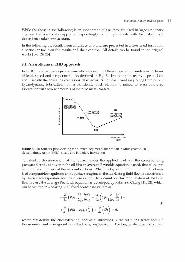
In an ICE, journal bearings are generally exposed to different operation conditions in termsof load, speed and temperature. As depicted in Fig. 3, depending on relative speed, loadand viscosity the operating conditions reflected as friction coefficient may range from purelyhydrodynamic lubrication with a sufficiently thick oil film to mixed or even boundarylubrication with severe amounts of metal to metal contact.

Figure 3. The Stribeck-plot showing the different regimes of lubrication: hydrodynamic (HD),elastohydrodynamic (EHD), mixed and boundary lubrication

To calculate the movement of the journal under the applied load and the correspondingpressure distribution within the oil film an average Reynolds equation is used, that takes intoaccount the roughness of the adjacent surfaces. When the typical minimum oil film thicknessis of comparable magnitude to the surface roughness, the lubricating fluid flow is also affectedby the surface asperities and their orientation. To account for this modification of the fluidflow we use the average Reynolds equation as developed by Patir and Cheng [21, 22], whichcan be written in a bearing shell fixed coordinate system as

− ∂

∂x

(θφx

h3

12ηp

∂p∂x

)− ∂

∂z

(θφz

h3

12ηp

∂p∂z

)+

+∂

∂x

(θ(h̄ + σsφs)

U2

)+

∂

∂t

(θh̄

)= 0,

(1)

where x, z denote the circumferential and axial directions, θ the oil filling factor and h, h̄the nominal and average oil film thickness, respectively. Further, U denotes the journal



circumferential speed, ηp the pressure dependent oil viscosity and σs the combined (root meansquare) surface roughness. φx, φz, φs represent the flow factors that actually take into accountthe influence of the surface roughness.

To describe mixed lubrication another process needs to be taken into account, namely the loadcarried by the surface asperities when metal-metal contact occurs.

The corresponding quantity is the asperity contact pressure pa and together with the areaexperiencing metal-metal contact, Aa, and the boundary friction coefficient μBound these yieldthe friction force RBound caused by asperity contact,

RBound = μBound · pa · Aa. (2)

To describe the metal-metal contact we use the Greenwood and Tripp approach [9], that isshortly outlined in the following.

The theory of Greenwood and Tripp is based on the contact of two nominally flat, randomrough surfaces. The asperity contact pressure pa is the product of the elastic factor K with aform function F5

2(Hs),

pa = KE∗F52(Hs), (3)

where Hs is a dimensionless clearance parameter, defined as Hs = h−δ̄sσs

, with σs being thecombined asperity summit roughness, which is calculated according to

σs =√

σ2s,J + σ2

s,S,

and δ̄s being the combined mean summit height, δ̄s = δ̄s,J + δ̄s,S, where the additionalsubscript J and S denotes the corresponding quantities of the journal and the bearing shell,

respectively. Further, E∗ denotes the composite elastic modulus, E∗ = (1−ν2

1E1

+1−ν2

2E2

)−1, whereνi and Ei are the Poisson ratio and Young’s modulus of the adjacent surfaces, respectively. Theform function is defined as

F52(Hs) =4.4086 · 10−5(4− Hs)

6.804 for Hs < 4

=0 for Hs ≥ 4,(4)

which shows that friction due to asperity contact sets in only for Hs < 4 and further sensiblydepends on the minimum oil film thickness as this quantity enters Eqn. 4 with almost 7thpower.

For the calculation of the Greenwood/Tripp parameters a 2D-profilometer trace was used thatwas performed on an run-in part of the bearing shell along the axial direction.

Modern engine oils include friction modifying additives like zinc dialkyl dithiophosphate(ZDTP) or Molybdenum based compounds to lower friction and wear in case metal-metalcontact occurs. For the Greenwood and Tripp contact model we employed in the following aboundary friction coefficient of μBound = 0.02.

The different contributions to friction, as listed in Eqs. (1) and (3), are generallynot independent from eachother. A reduction in lubricant viscosity, while decreasing



hydrodynamic losses, may cause - depending on the load - an overly increase in asperitycontact as the oil film thickness enters Eq. (4) with almost 7th power.

3.1.1. Testing Method

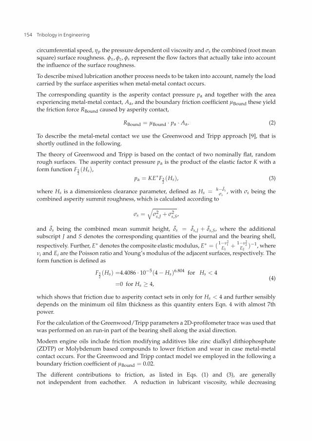
Figure 4. left: schematic drawing of the journal bearing test rig LP06: test part denotes the location of thetest bearing, torque sensor the HBM T10F sensor used for friction moment measurement. Right: Drawingof the test con rod with test bearing showing the location of the temperatures sensors: T2 sits in thecenter at 0◦ circumferential angle, with T1 and T3 at ±45◦ circumferential angle, respectively.

MIBA2’s journal bearing test rig LP06 was used for the experimental measurements. It issketched in Fig. 4 and consists of a heavy, elastically mounted base plate which carries thetwo support blocks, the test con rod with the hydraulic actuator and the driveshaft attachedto the electric drive mechanism. The hydraulic actuator applies the load along the verticaldirection, which is consequently defined as 0◦ circumferential angle.

The friction torques arising from all three journal bearings were measured at the driveshaft; forthe comparisons load cycle averaged values of the friction moment (the load cycle is depictedin Fig. 5) are used.

The LP06 is equipped with a number of temperature sensors to capture the occurringtemperatures at various points of the test rig; to this task temperature is measured by usingthermocouple elements of type K that have an accuracy of ±1◦C. Besides two temperaturesin the con rod and the oil outflow temperature, the bearing shell temperatures of the test andsupport bearings are measured at three different points at the back of each correspondingbearing shell. As shown in Fig. 4, two of these temperature sensors are located at ±45◦circumferential angle from the vertical axis and the third in the middle at 0◦ circumferentialangle.

For the bearing tests following conditions were maintained: for test- and support-bearingssteel-supported leaded bronce trimetal bearings with a sputter overlay were employed; foreach test-run new bearings with an inner diameter of 76 mm and a width of 34 mm were usedand mounted into the test rig with a nominal clearance of 0.04 mm (10/00 relative clearance). Ahydraulic attenuator applied the transient loads with the corresponding peak loads of either

2 MIBA Bearing Group, Dr.-Mitterbauer-Str. 3 4663 Laakirchen, Austria



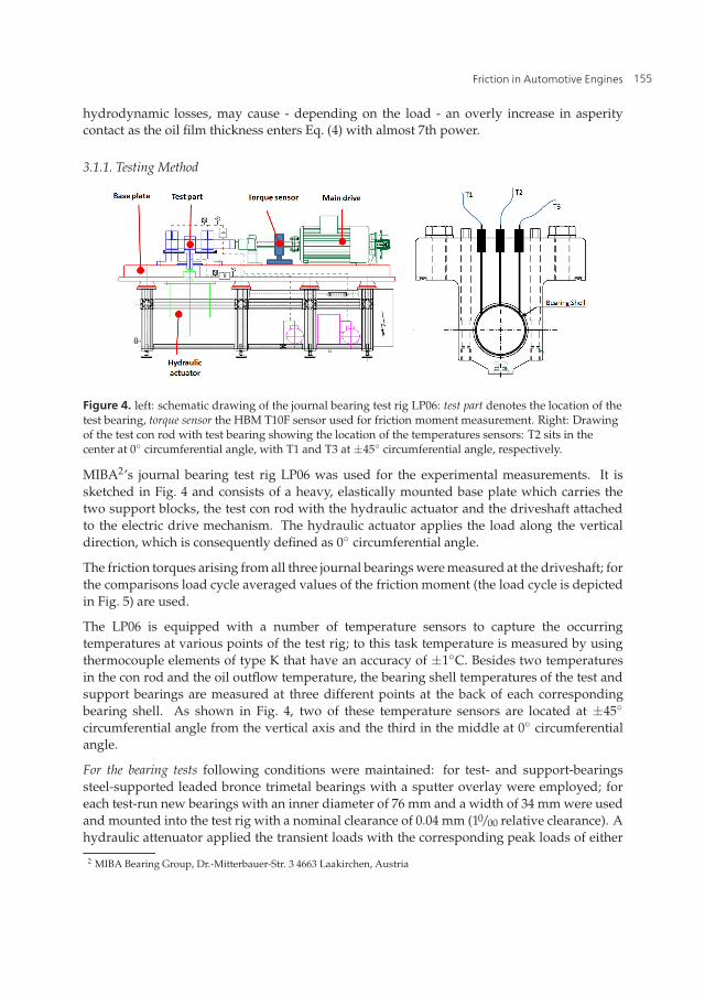
Figure 5. Plot of the loads applied to the test bearing: at a frequency of 50 Hz a sinusoidal load is appliedalong the vertical direction with a preload of -10kN and a peak load of either 180 kN for the 70 MPa loadcase (shown as solid black line) or a peak load of 106 kN for the 41 MPa load case (red dashed line).

41 MPa, 54 MPa, 70 MPa or 76 MPa. For a convenient comparison of the results to otherworks the peak load is expressed in MPa to account for the involved bearing dimensions.This is conducted by dividing the load force by the projected bearing area (product of bearingwidth and bearing diameter). Therefore, the peak loads of 106 kN and 180 kN correspondto 41 MPa or 70 MPa, respectively, for the present bearing dimensions (see also Fig. 5). Inthe following, the corresponding peak loads are used to distinguish between the differenttransient load cases.

The different oils were preconditioned to 80±5◦C inflow temperature. After the test-run thewear at several points in the journal bearings was measured and the so obtained wear profileswere included in the simulation model.

3.1.2. Simulation

For the simulation a model of the LP06 was setup within an elastic multi-body dynamicssolver (AVL-Excite Powerunit3). The simulation model consists of the test con rod includingthe test bearing, the two support-blocks with journal bearings and the shaft running freely,but supported by the adjacent bearings. All structure parts are modeled as dynamicallycondensed finite element (FE)-structures.

The three journal bearings, 76mm in diameter and 34mm width, are represented as EHD orTEHD-joints, respectively.

To obtain realistic dynamic lubricant viscosities for the calculations, the viscosities anddensities of fresh SAE10/SAE20/SAE30 and SAE40 monograde oils were measured atdifferent temperatures in the OMV-laboratory4. To obtain a pressure dependent oil-modelfor the simulation, the pressure dependency was impressed onto the measured viscosities by

3 AVL List GmbH, Advanced Simulation Technology, Hans-List-Platz 1, 8020 Graz, Austria4 OMV Refining & Marketing GmbH, Uferstrasse 8, 1220 Wien, Austria



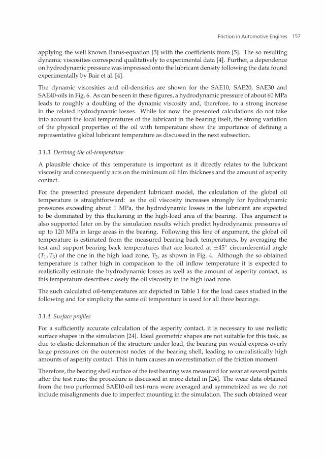
applying the well known Barus-equation [5] with the coefficients from [5]. The so resultingdynamic viscosities correspond qualitatively to experimental data [4]. Further, a dependenceon hydrodynamic pressure was impressed onto the lubricant density following the data foundexperimentally by Bair et al. [4].

The dynamic viscosities and oil-densities are shown for the SAE10, SAE20, SAE30 andSAE40-oils in Fig. 6. As can be seen in these figures, a hydrodynamic pressure of about 60 MPaleads to roughly a doubling of the dynamic viscosity and, therefore, to a strong increasein the related hydrodynamic losses. While for now the presented calculations do not takeinto account the local temperatures of the lubricant in the bearing itself, the strong variationof the physical properties of the oil with temperature show the importance of defining arepresentative global lubricant temperature as discussed in the next subsection.

3.1.3. Deriving the oil-temperature

A plausible choice of this temperature is important as it directly relates to the lubricantviscosity and consequently acts on the minimum oil film thickness and the amount of asperitycontact.

For the presented pressure dependent lubricant model, the calculation of the global oiltemperature is straightforward: as the oil viscosity increases strongly for hydrodynamicpressures exceeding about 1 MPa, the hydrodynamic losses in the lubricant are expectedto be dominated by this thickening in the high-load area of the bearing. This argument isalso supported later on by the simulation results which predict hydrodynamic pressures ofup to 120 MPa in large areas in the bearing. Following this line of argument, the global oiltemperature is estimated from the measured bearing back temperatures, by averaging thetest and support bearing back temperatures that are located at ±45◦ circumferential angle(T1, T3) of the one in the high load zone, T2, as shown in Fig. 4. Although the so obtainedtemperature is rather high in comparison to the oil inflow temperature it is expected torealistically estimate the hydrodynamic losses as well as the amount of asperity contact, asthis temperature describes closely the oil viscosity in the high load zone.

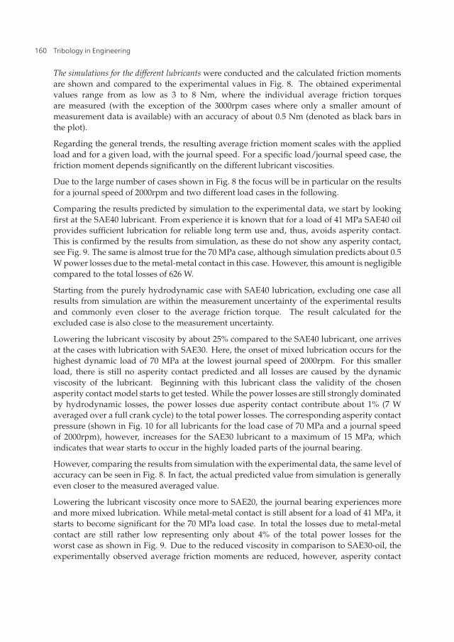
The such calculated oil-temperatures are depicted in Table 1 for the load cases studied in thefollowing and for simplicity the same oil temperature is used for all three bearings.

3.1.4. Surface profiles

For a sufficiently accurate calculation of the asperity contact, it is necessary to use realisticsurface shapes in the simulation [24]. Ideal geometric shapes are not suitable for this task, asdue to elastic deformation of the structure under load, the bearing pin would express overlylarge pressures on the outermost nodes of the bearing shell, leading to unrealistically highamounts of asperity contact. This in turn causes an overestimation of the friction moment.

Therefore, the bearing shell surface of the test bearing was measured for wear at several pointsafter the test runs; the procedure is discussed in more detail in [24]. The wear data obtainedfrom the two performed SAE10-oil test-runs were averaged and symmetrized as we do notinclude misalignments due to imperfect mounting in the simulation. The such obtained wear



(a) (e)

(b) (f)

(c) (g)

(d) (h)

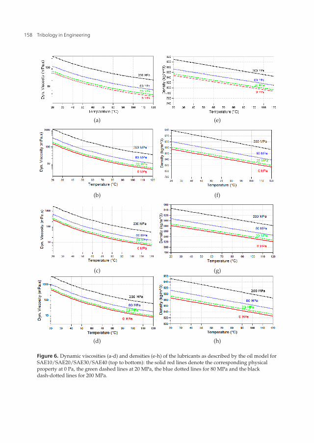
Figure 6. Dynamic viscosities (a-d) and densities (e-h) of the lubricants as described by the oil model forSAE10/SAE20/SAE30/SAE40 (top to bottom): the solid red lines denote the corresponding physicalproperty at 0 Pa, the green dashed lines at 20 MPa, the blue dotted lines for 80 MPa and the blackdash-dotted lines for 200 MPa.



SAE10 T41MPa T70MPa[◦C] [◦C]

87.4 94.6


89.2 96.8


89.8 97.9


91.8 99.6

Table 1. Calculated oil-temperatures (see text) for the studied load cases (denoted as subscript) and thedifferent oils.

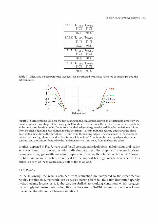
Figure 7. Surface profile used for the test bearing in the simulation, shown as deviation (in μm) from thenominal geometrical shape of the bearing shell for different axial cuts: the red line denotes the deviationat the outermost bearing nodes, 0mm from the shell edges, the green dashed line the deviation −1.4mmfrom the shell edges, the blue dotted line the deviation −2.7mm from the bearing edges and the blackdash-dotted line shows the deviation −4.1mm from the bearing edges. The deviations in the middle ofthe journal bearing, along axial direction from −4.1mm to −17mm from the bearing edges, stay ratherconstant and are almost identical to the deviation for −4.1mm away from the bearing edges.

profiles, depicted in Fig. 7, were used for all consequent calculations (all lubricants and loads)as it was found that the results with individual wear profiles prepared for every lubricantcaused only negligible differences in comparison to the results obtained with the SAE10-wearprofile. Similar wear profiles were used for the support bearings, which, however, are lesscritical as each of these carries only half of the total load.

3.1.5. Results

In the following, the results obtained from simulation are compared to the experimentalresults. For this task, the results are discussed starting from full fluid film lubrication (purelyhydrodynamic losses), as it is the case for SAE40, to working conditions which progressincreasingly into mixed lubrication, like it is the case for SAE10, where friction power lossesdue to metal-metal contact become significant.



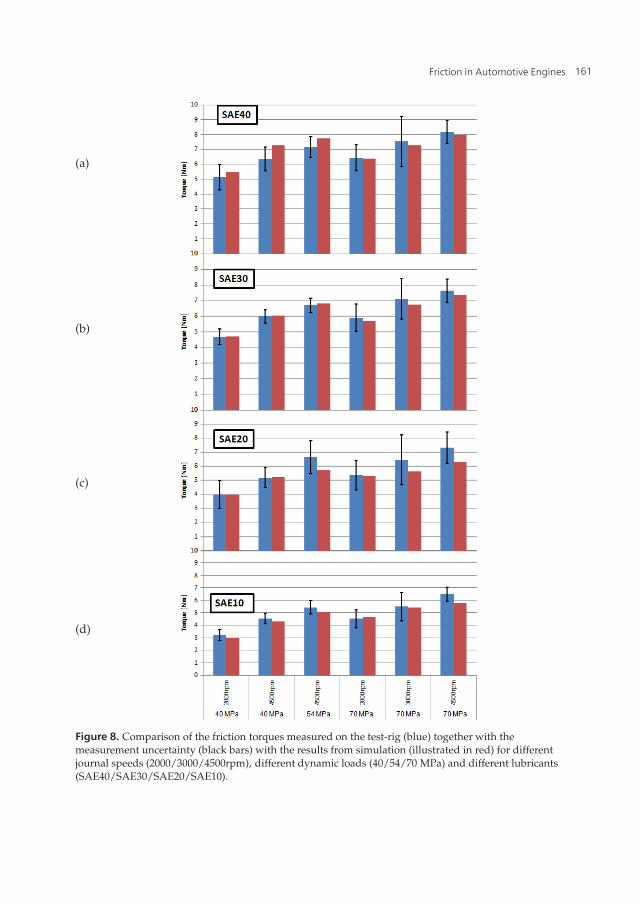
The simulations for the different lubricants were conducted and the calculated friction momentsare shown and compared to the experimental values in Fig. 8. The obtained experimentalvalues range from as low as 3 to 8 Nm, where the individual average friction torquesare measured (with the exception of the 3000rpm cases where only a smaller amount ofmeasurement data is available) with an accuracy of about 0.5 Nm (denoted as black bars inthe plot).

Regarding the general trends, the resulting average friction moment scales with the appliedload and for a given load, with the journal speed. For a specific load/journal speed case, thefriction moment depends significantly on the different lubricant viscosities.

Due to the large number of cases shown in Fig. 8 the focus will be in particular on the resultsfor a journal speed of 2000rpm and two different load cases in the following.

Comparing the results predicted by simulation to the experimental data, we start by lookingfirst at the SAE40 lubricant. From experience it is known that for a load of 41 MPa SAE40 oilprovides sufficient lubrication for reliable long term use and, thus, avoids asperity contact.This is confirmed by the results from simulation, as these do not show any asperity contact,see Fig. 9. The same is almost true for the 70 MPa case, although simulation predicts about 0.5W power losses due to the metal-metal contact in this case. However, this amount is negligiblecompared to the total losses of 626 W.

Starting from the purely hydrodynamic case with SAE40 lubrication, excluding one case allresults from simulation are within the measurement uncertainty of the experimental resultsand commonly even closer to the average friction torque. The result calculated for theexcluded case is also close to the measurement uncertainty.

Lowering the lubricant viscosity by about 25% compared to the SAE40 lubricant, one arrivesat the cases with lubrication with SAE30. Here, the onset of mixed lubrication occurs for thehighest dynamic load of 70 MPa at the lowest journal speed of 2000rpm. For this smallerload, there is still no asperity contact predicted and all losses are caused by the dynamicviscosity of the lubricant. Beginning with this lubricant class the validity of the chosenasperity contact model starts to get tested. While the power losses are still strongly dominatedby hydrodynamic losses, the power losses due asperity contact contribute about 1% (7 Waveraged over a full crank cycle) to the total power losses. The corresponding asperity contactpressure (shown in Fig. 10 for all lubricants for the load case of 70 MPa and a journal speedof 2000rpm), however, increases for the SAE30 lubricant to a maximum of 15 MPa, whichindicates that wear starts to occur in the highly loaded parts of the journal bearing.

However, comparing the results from simulation with the experimental data, the same level ofaccuracy can be seen in Fig. 8. In fact, the actual predicted value from simulation is generallyeven closer to the measured averaged value.

Lowering the lubricant viscosity once more to SAE20, the journal bearing experiences moreand more mixed lubrication. While metal-metal contact is still absent for a load of 41 MPa, itstarts to become significant for the 70 MPa load case. In total the losses due to metal-metalcontact are still rather low representing only about 4% of the total power losses for theworst case as shown in Fig. 9. Due to the reduced viscosity in comparison to SAE30-oil, theexperimentally observed average friction moments are reduced, however, asperity contact



(a)

(b)

(c)

(d)

Figure 8. Comparison of the friction torques measured on the test-rig (blue) together with themeasurement uncertainty (black bars) with the results from simulation (illustrated in red) for differentjournal speeds (2000/3000/4500rpm), different dynamic loads (40/54/70 MPa) and different lubricants(SAE40/SAE30/SAE20/SAE10).



(a) (b)

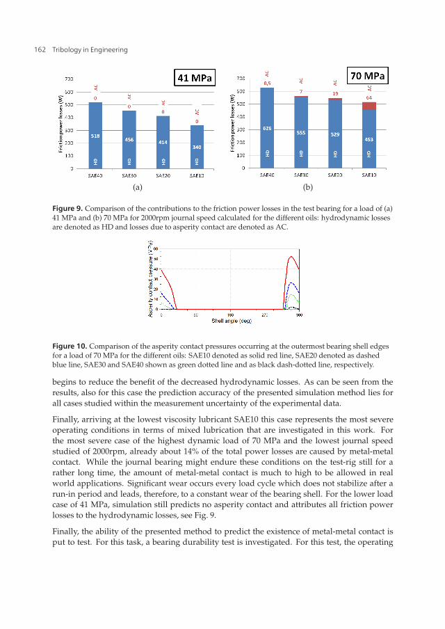
Figure 9. Comparison of the contributions to the friction power losses in the test bearing for a load of (a)41 MPa and (b) 70 MPa for 2000rpm journal speed calculated for the different oils: hydrodynamic lossesare denoted as HD and losses due to asperity contact are denoted as AC.

Figure 10. Comparison of the asperity contact pressures occurring at the outermost bearing shell edgesfor a load of 70 MPa for the different oils: SAE10 denoted as solid red line, SAE20 denoted as dashedblue line, SAE30 and SAE40 shown as green dotted line and as black dash-dotted line, respectively.

begins to reduce the benefit of the decreased hydrodynamic losses. As can be seen from theresults, also for this case the prediction accuracy of the presented simulation method lies forall cases studied within the measurement uncertainty of the experimental data.

Finally, arriving at the lowest viscosity lubricant SAE10 this case represents the most severeoperating conditions in terms of mixed lubrication that are investigated in this work. Forthe most severe case of the highest dynamic load of 70 MPa and the lowest journal speedstudied of 2000rpm, already about 14% of the total power losses are caused by metal-metalcontact. While the journal bearing might endure these conditions on the test-rig still for arather long time, the amount of metal-metal contact is much to high to be allowed in realworld applications. Significant wear occurs every load cycle which does not stabilize after arun-in period and leads, therefore, to a constant wear of the bearing shell. For the lower loadcase of 41 MPa, simulation still predicts no asperity contact and attributes all friction powerlosses to the hydrodynamic losses, see Fig. 9.

Finally, the ability of the presented method to predict the existence of metal-metal contact isput to test. For this task, a bearing durability test is investigated. For this test, the operating



conditions are made even more severe by increasing the dynamic load to a maximum of 76MPa at a journal speed of 3000rpm and increasing the oil inflow temperature of the SAE10lubricant to 110◦C. In comparison to the previous operating conditions with an oil inflowtemperature of 80◦C, this temperature increase causes the lubricant viscosity to decrease bymore than 50% (see Fig. 6). These operating conditions lead consequently to bearing shelltemperatures exceeding 130◦C. As significant metal-metal contact occurs for these operatingconditions, it can be detected by contact voltage measurements. For this measurement, avoltage is applied e.g. in form of a charged capacitor between the journal and the bearing.As the lubricant has only a poor electrical conductivity, the capacitor stays charged and thevoltage remains unchanged. When metal-metal occurs, the capacitor can discharge due tothe corresponding increased electrical conductivity; this process can be observed as change(decrease) of the voltage.

A comparison of the experimental contact voltage measurement and the predictedmetal-metal contact is shown in Fig. 11 together with the applied dynamic load. It can be seenthat when the load exceeds a certain threshold, metal-metal contact occurs. When comparedto the results from simulation, the onset and the duration of the calculated metal metal contactagrees very well with the measured contact voltage data.

Overall, the presented simulation method appears to describe the actual processes in thejournal bearing sufficiently well, as it predicts the friction moment accurately and reliably overa large range of working conditions, which range from purely hydrodynamic to significantlymixed lubrication.

Other important properties related to reliability in lubricated journal bearings are the peak oilfilm pressure (POFP) and the minimum oil film thickness (MOFT) [18, 20], that are depictedin Figs. 12 and 13 for the investigated lubricants.

As shown in Fig. 12, the POFPs change significantly from about 90 MPa to 120 MPa betweenthe two different loads, but do not vary significantly between the different lubricants at thesame load.

For a load of 41 MPa the results show that the MOFT is for all investigated oil-classes above 1.5μm, which is the asperity contact threshold. Therefore, no metal-metal contact occurs, whichcan also be seen in the power losses shown in Fig. 9.

Further, it is interesting to note that the MOFT decreases by about 0.5 μm for every decreasein SAE-class; while the MOFT is considerably large with 3 μm at the point of maximumload for lubrication with SAE40, it decreases to about 2.5 μm and 2.0 μm for SAE30 andSAE20, respectively. For SAE10 the MOFT at the point of maximum load decreases further toabout 1.5 μm; while from simulation still no asperity contact occurs for this case, in practicalapplications other effects not included here, like journal misalignment may lead to asperitycontact.

The situation is quite different for a load of 70 MPa where all oils cannot avoid a certainamount of asperity contact and the MOFT consequently drops for all oils below 1.5 μm,however, for a different number of degrees crank angle. It is instructive to note that for aload of 70 MPa the MOFT changes not by the same amount between the different viscosityclasses as for the 41 MPa load case. This can be explained by the choice of the elastic factor in



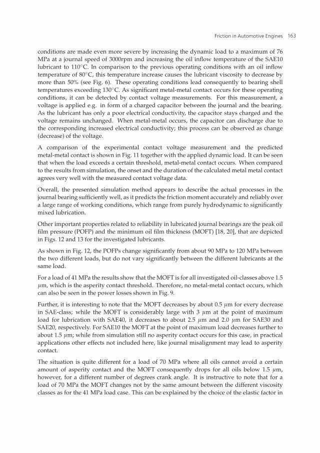
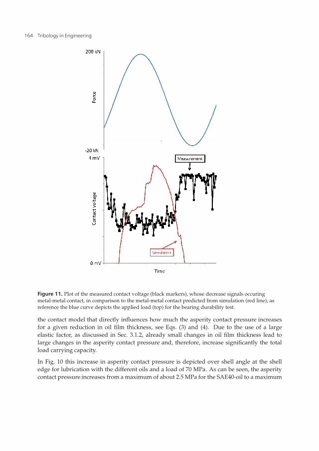
Figure 11. Plot of the measured contact voltage (black markers), whose decrease signals occuringmetal-metal contact, in comparison to the metal-metal contact predicted from simulation (red line); asreference the blue curve depicts the applied load (top) for the bearing durability test.

the contact model that directly influences how much the asperity contact pressure increasesfor a given reduction in oil film thickness, see Eqs. (3) and (4). Due to the use of a largeelastic factor, as discussed in Sec. 3.1.2, already small changes in oil film thickness lead tolarge changes in the asperity contact pressure and, therefore, increase significantly the totalload carrying capacity.

In Fig. 10 this increase in asperity contact pressure is depicted over shell angle at the shelledge for lubrication with the different oils and a load of 70 MPa. As can be seen, the asperitycontact pressure increases from a maximum of about 2.5 MPa for the SAE40-oil to a maximum



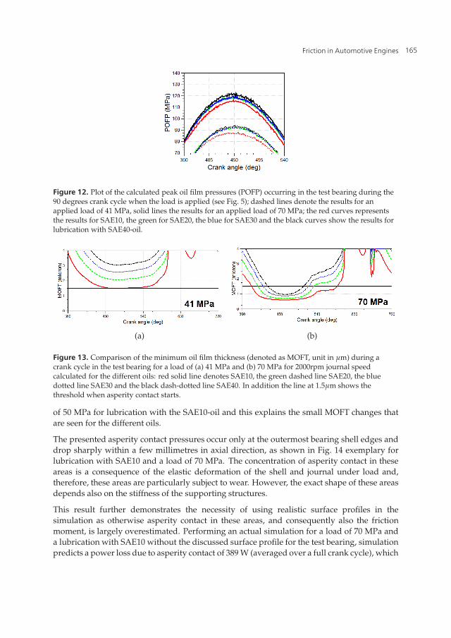
Figure 12. Plot of the calculated peak oil film pressures (POFP) occurring in the test bearing during the90 degrees crank cycle when the load is applied (see Fig. 5); dashed lines denote the results for anapplied load of 41 MPa, solid lines the results for an applied load of 70 MPa; the red curves representsthe results for SAE10, the green for SAE20, the blue for SAE30 and the black curves show the results forlubrication with SAE40-oil.

(a) (b)

Figure 13. Comparison of the minimum oil film thickness (denoted as MOFT, unit in μm) during acrank cycle in the test bearing for a load of (a) 41 MPa and (b) 70 MPa for 2000rpm journal speedcalculated for the different oils: red solid line denotes SAE10, the green dashed line SAE20, the bluedotted line SAE30 and the black dash-dotted line SAE40. In addition the line at 1.5μm shows thethreshold when asperity contact starts.

of 50 MPa for lubrication with the SAE10-oil and this explains the small MOFT changes thatare seen for the different oils.

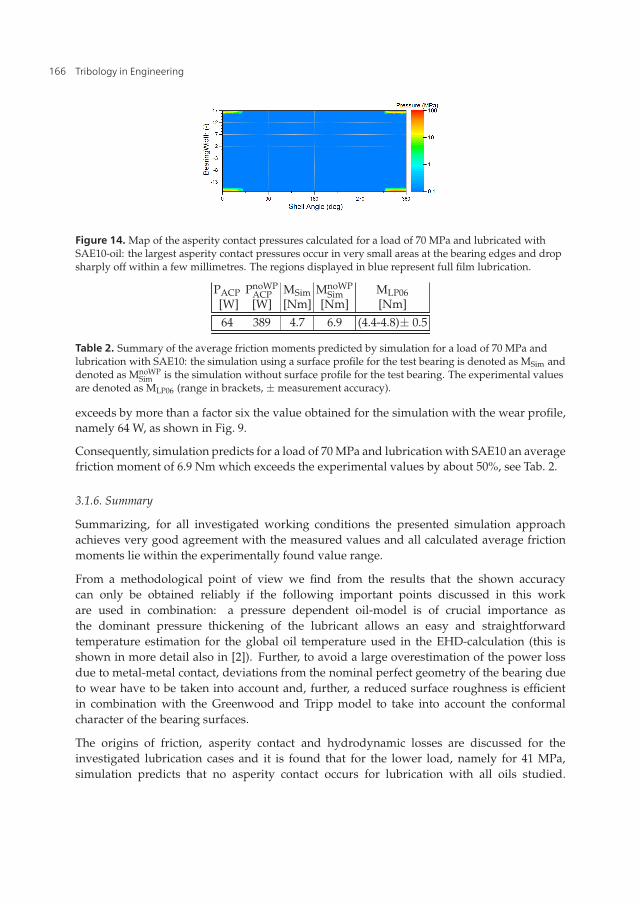
The presented asperity contact pressures occur only at the outermost bearing shell edges anddrop sharply within a few millimetres in axial direction, as shown in Fig. 14 exemplary forlubrication with SAE10 and a load of 70 MPa. The concentration of asperity contact in theseareas is a consequence of the elastic deformation of the shell and journal under load and,therefore, these areas are particularly subject to wear. However, the exact shape of these areasdepends also on the stiffness of the supporting structures.

This result further demonstrates the necessity of using realistic surface profiles in thesimulation as otherwise asperity contact in these areas, and consequently also the frictionmoment, is largely overestimated. Performing an actual simulation for a load of 70 MPa anda lubrication with SAE10 without the discussed surface profile for the test bearing, simulationpredicts a power loss due to asperity contact of 389 W (averaged over a full crank cycle), which



Figure 14. Map of the asperity contact pressures calculated for a load of 70 MPa and lubricated withSAE10-oil: the largest asperity contact pressures occur in very small areas at the bearing edges and dropsharply off within a few millimetres. The regions displayed in blue represent full film lubrication.

PACP PnoWPACP MSim MnoWP

Sim MLP06[W] [W] [Nm] [Nm] [Nm]

64 389 4.7 6.9 (4.4-4.8)± 0.5

Table 2. Summary of the average friction moments predicted by simulation for a load of 70 MPa andlubrication with SAE10: the simulation using a surface profile for the test bearing is denoted as MSim anddenoted as MnoWP

Sim is the simulation without surface profile for the test bearing. The experimental valuesare denoted as MLP06 (range in brackets, ±measurement accuracy).

exceeds by more than a factor six the value obtained for the simulation with the wear profile,namely 64 W, as shown in Fig. 9.

Consequently, simulation predicts for a load of 70 MPa and lubrication with SAE10 an averagefriction moment of 6.9 Nm which exceeds the experimental values by about 50%, see Tab. 2.

3.1.6. Summary

Summarizing, for all investigated working conditions the presented simulation approachachieves very good agreement with the measured values and all calculated average frictionmoments lie within the experimentally found value range.

From a methodological point of view we find from the results that the shown accuracycan only be obtained reliably if the following important points discussed in this workare used in combination: a pressure dependent oil-model is of crucial importance asthe dominant pressure thickening of the lubricant allows an easy and straightforwardtemperature estimation for the global oil temperature used in the EHD-calculation (this isshown in more detail also in [2]). Further, to avoid a large overestimation of the power lossdue to metal-metal contact, deviations from the nominal perfect geometry of the bearing dueto wear have to be taken into account and, further, a reduced surface roughness is efficientin combination with the Greenwood and Tripp model to take into account the conformalcharacter of the bearing surfaces.

The origins of friction, asperity contact and hydrodynamic losses are discussed for theinvestigated lubrication cases and it is found that for the lower load, namely for 41 MPa,simulation predicts that no asperity contact occurs for lubrication with all oils studied.



Though the minimum oil film thickness found in simulation for SAE10 is very close to thethreshold of asperity contact, all investigated oils are expected to provide sufficient lubricationfor this load. The correspondingly calculated friction power losses demonstrate well theattainable friction reduction by choosing a lubricant with the optimum viscosity for a certainload; in particular, for a load of 41 MPa the friction power losses can be reduced from 518 Wfor SAE40 down to 340 W for SAE10, which is a reduction by 33%.

For the significantly more severe load case of 70 MPa, a certain amount of asperity contactis seen for all studied oils in the results from simulation. Indeed, the hydrodynamic frictionpower losses could be reduced from 626 W for the SAE40 oil to 453 W calculated for the SAE10oil, which corresponds theoretically to almost a 30% reduction in friction. However, powerlosses caused by metal metal contact diminish this potential by a certain extent. Still, thetotal friction power losses are reduced from 626.5 W for SAE40 to 517 W for SAE10, which isstill a reduction by almost 20%. This result demonstrates the efficiency in reducing friction bychoosing a lubricant with reduced viscosity, so that, as long as measures to maintain reliabilityare taken (e.g. by using antiwear-additives in the lubricant), even a small amount of asperitycontact might be tolerated to reduce the total friction power losses. This result is the startingpoint for the further work in Sec. 4

3.2. Including thermal processes - TEHD

Although the agreement of the previously presented simulation method with theexperimental data is very much on spot and within the experimental accuracy for thewhole range of working conditions studied, the neglect of local temperatures is a roughapproximation of reality and its deviations to a model including local temperatures needto be quantified. In the following the isothermal simulation method is extended toa thermoelastohydrodynamic (TEHD) calculation to consider local temperatures. Whilecritically important information like the bearing shell back temperatures was needed as inputfor the EHD simulation, these should now emerge from a representative thermal submodel.Due to the fact that the extension to TEHD is not straightforward and its thermal submodeladds a number of additional uncertain factors, the boundary conditions are chosen not onlyon a basis of physical arguments but also sufficiently distant from the oil film to minimizetheir influence on the results.

In the following the focus is on the extension of the isothermal simulation method to includelocal temperatures; therefore, all details regarding the experimental part are not repeated, butcan be found in Section 3.1.

3.2.1. Theory

From a methodological point of view the TEHD-approach to journal bearings is well known;it adds the energy equation and heat equation to the set of differential equation that need tobe solved together. While this approach represents a more complete picture of the physicalprocesses in journal bearings, it has several severe drawbacks. While the dramaticallyincreased cpu-time is more of a practical drawback that might be resolved by faster computersor faster solvers, the required thermal submodel needs a detailed knowledge of the thermal



properties and of the heat flows of the test-rig. Therefore, subsection 3.2.4 is devoted to discussits derivation.

Following [17] the Reynolds equation is combined with the energy equation to be able to takethermal processes into account. In a body shell fixed coordinate system such an extendedReynolds equation can be defined as [17, 23]

− ∂

∂x

(θα2 ∂p

∂x

)− ∂

∂z

(θα2 ∂p

∂z

)+

+∂

∂x

(θβ

)+

∂

∂t

(θγ

)= 0,

(5)

where x, z denote the circumferential and axial directions and θ the oil filling factor. α, β, γ aredefined as

−α2 = h3 ·∫ 1

0ρ

( ∫ y

0

y′η′ dy′ −

∫ 10

y′η′ dy′∫ 1

01η′ dy′

·∫ y

0

1η′ dy′

)dy

β = h ·U∫ 1

0ρ

(1−

∫ y0

1η′ dy′∫ 1

01η′ dy′

)dy

γ = h∫ 1

0ρ dy,

(6)

where the direction along the film height, y, is normalized to the oil film height h, thus theintegration is carried out from 0 to 1. Further, the prime (′) indicates that the correspondingquantity depends on y′. U is the difference of the circumferential speeds of journal and bearingshell, U = UShell −UJournal. η and ρ denote the oil viscosity and density, both are consideredas pressure and temperature dependent.

The extended Reynolds equation (5) is solved together with the energy equation for the fluidfilm that is extended with the term f (Asp) to include heating due to asperity contact,

ρcp

{∂T∂t

+ u∂T∂x

+ w∂T∂z

+1h

[v− y(

∂h∂t

+ u∂h∂x

+ w∂h∂z

)

]∂T∂y

}

+Tρ

∂ρ

∂T

(∂p∂t

+ u∂p∂x

+ w∂p∂z

)− κ

h2∂2T∂y2

=η

h2

[(∂u∂y

)2

+

(∂w∂y

)2]+ f (Asp),

(7)

where κ denotes the thermal conductivity, u, v, w refer to the (x, y, z) components of the fluidvelocity vector v at the corresponding fluid point and cp represents the specific heat of the



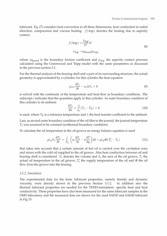
lubricant. Eq. (7) considers heat convection in all three dimensions, heat conduction in radialdirection, compression and viscous heating. f (Asp) denotes the heating due to asperitycontact,

f (Asp) =τAsp

h3 U

τAsp =μBoundpAsp,

(8)

where μBound is the boundary friction coefficient and pAsp the asperity contact pressurecalculated using the Greenwood and Tripp model with the same parameters as discussedin the previous section 3.1.

For the thermal analysis of the bearing shell and a part of its surrounding structure, the actualgeometry is approximated by a cylinder; for this cylinder the heat equation

ρscs∂Ts

∂t− κsΔTs = 0 (9)

is solved with the continuity of the temperature and heat flow as boundary conditions. Thesubscript s indicates that the quantities apply to this cylinder. As outer boundary condition ofthis cylinder to its ambient

∂Ts

∂n+

λ

κs(Ts − TR) = 0 (10)

is used, where TR is a reference temperature and λ the heat transfer coefficient to the ambient.

Last, as second outer boundary condition of the oil film to the journal, the journal temperatureTJ was assumed to be constant (isothermal boundary condition).

To calculate the oil temperature in the oil groove an energy balance equation is used

ρcpVo∂To

∂t=

∫So

(κs

∂Ts

∂r− κ

∂T∂y

)dS + ρcpΦ(T′o − To) (11)

that takes into account that a certain amount of hot oil is carried over the cavitation zoneand mixes with the cold oil supplied to the oil groove. Also heat conduction between oil andbearing shell is considered. Vo denotes the volume and So the area of the oil groove, To theactual oil temperature in the oil groove, T′o the supply temperature of the oil and Φ the oilflow from the groove into the bearing.

3.2.2. Simulation

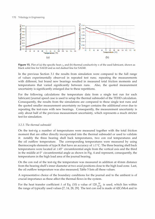
The experimental data for the basic lubricant properties, namely density and dynamicviscosity, were already shown in the previous Section 3.1.2. In addition also thethermal lubricant properties are needed for the TEHD-simulation: specific heat and heatconductivity. These properties have also been measured for the same lubricant samples in theOMV-laboratory and the measured data are shown for the used SAE20 and SAE40 lubricantin Fig 15.



(a) (b)

Figure 15. Plot of (a) the specific heat cp and (b) thermal conductivity κ of the used lubricant, shown asblack solid line for SAE20 and as red dashed line for SAE40.

In the previous Section 3.1 the results from simulation were compared to the full rangeof values experimentally observed in repeated test runs; repeating the measurementswith different, but brand new bearings resulted in measured total friction moments andtemperatures that varied significantly between runs. Also, the quoted measurementuncertainty is significantly enlarged due to these repetitions.

For the following calculations the temperature data from a single test run for eachlubricant/journal speed case is used to setup the thermal submodel of the TEHD calculation.Consequently, the results from the simulations are compared to these single test runs andthe quoted smaller measurement uncertainty no longer contains the additional error due torepeating the test-runs with new bearings. Consequently, the measurement uncertainty isonly about half of the previous measurement uncertainty, which represents a much strictertest for simulation.

3.2.3. The thermal submodel

On the test-rig a number of temperatures were measured together with the total frictionmoment that are either directly incorporated into the thermal submodel or used to validateit: notably the three bearing shell back temperatures, two con rod temperatures andthe oil outflow temperature. The corresponding temperatures were measured by usingthermocouple elements of type K that have an accuracy of ±1◦C. The three bearing shell backtemperatures were located at ±45◦ circumferential angle from the vertical axis and the thirdin the middle at 0◦ circumferential angle as shown in Fig. 4 and represent, consequently, thetemperatures in the high load area of the journal bearing.

On the con rod of the test-rig the temperature was measured in addition at 41mm distancefrom the bearing shell’s inner diameter at two axial positions close to the high load zone. Last,the oil outflow temperature was also measured; Table 5 lists all these values.

A representative choice of the boundary conditions for the journal and to the ambient is ofcrucial importance as these affect the thermal flows in the system.

For the heat transfer coefficient λ of Eq. (10) a value of 120 Wm2K is used, which lies within

the range of typically used values [7, 14, 28, 29]. The test con rod is made of 42CrMo4 and to



describe its thermal behaviour a thermal conductivity of κs = 46 Wm K and specific heat capacity

of cs = 460.5 Jkg K are used (see also Table 3).

Further, the journal is assumed to be isothermal which sufficiently well approximates the realsurface temperature as its circumferential speed is significantly larger than typical heat flowprocesses [17]. The journal temperature TJ is the only adjustable property in the simulationmodel and it is chosen such that the calculated bearing shell back temperatures averaged overone cycle, TSim

1 , TSim2 , TSim

3 , agree well with the corresponding experimental values (TExp1 , TExp

2 ,

TExp3 ), see Table 5.

Outward of the oil film 25 mm of the surrounding structure are taken into account in thethermal analysis; as reference temperature, denoted as TR in Eq. (10), a value is used thatwas measured in the con rod of the test-rig at 41 mm distance from the bearing shell’s innerdiameter at two axial positions close to the high load zone. The used values for TR, obtainedby averaging the aforementioned two experimental values, are listed in Table 4.

The current model does not account for thermoelastic deformations and the consequentchanges in bearing clearance. In the previous EHD-simulations a value for the bearingclearance was used that was measured experimentally at room temperature. While thissimplification appears not to significantly affect the calculation of the total friction moment,the in this way calculated oil flow through the bearing does not agree well with the actualexperimental oil flow. Therefore, the thermal power leaving the bearing with the oil-outflowcannot be expected to be calculated reliably. As consequence, it is attempted in the followingto at least partially include thermoelastic effects by scaling the bearing clearance in theTEHD-calculations such that the oil flow through the bearing agrees with the experimentallycontrolled oil-flow of 2 litres per minute.

Further, it appears from the results that the such adapted bearing clearance has no other majorimpacts on the thermal submodel as the bearing shell temperatures experience only singledegree changes.

As the amount of oil flow through the bearing is then properly included in the simulation, thisfurther allows to calculate an approximative value5 of the mean oil outflow temperature dueto the power losses in the bearing and compare this value to the corresponding measured oiloutflow temperature.

The mean temperature increase of the lubricant after flowing through the bearing, ΔT, iscalculated using the thermal power leaving the bearing with the lubricant, Poil out, using

ΔT =Poil out

cpρ

(Vt

)−1

, (12)

where c and ρ denote the specific heat capacity and density of the lubricant, respectively,and V

t is the oil volume flow through the bearing. The approximative mean oil outflow

5 As we use a commercial software package we do not have access to the required numerical data to realize an exactscheme.



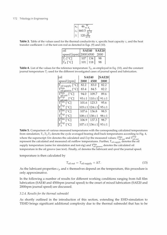
κs 46 Wm K

cs 460.5 Jkg K

λ 120 Wm2K

Table 3. Table of the values used for the thermal conductivity κ, specific heat capacity cs and the heattransfer coefficient λ of the test con-rod as denoted in Eqs. (9) and (10).

oil SAE40 SAE20speed [rpm] 2000 4500 2000TJ [◦C] 107 134 98TR [◦C] 101 118 98

Table 4. List of the values for the reference temperature TR, as employed in Eq. (10), and the constantjournal temperature TJ used for the different investigated cases of journal speed and lubrication.

oil SAE40 SAE20speed [rpm] 2000 4500 2000Toil supply [◦C] 82.2 83.0 82.2TSim

oil groove [◦C] 83.4 84.5 82.2

TSimoil out [◦C] 94.0 109.7 89.6

TExpoil out [◦C] 93±1 110±1 91±1

TSim1 [◦C] 101.6 123.3 95.6

TExp1 [◦C] 103±1 124±1 95±1

TSim2 [◦C] 107.6 136.8 98.5

TExp2 [◦C] 108±1 138±1 98±1

TSim3 [◦C] 106.9 137.3 98.7

TExp3 [◦C] 107±1 136±1 93±1

Table 5. Comparison of various measured temperatures with the corresponding calculated temperaturesfrom simulation; T1,T2,T3 denote the cycle averaged bearing shell back temperatures according to Fig. 4,where the superscript Sim denotes the calculated and Exp the measured values; TSim

oil out and TExpoil out

represent the calculated and measured oil outflow temperatures. Further, Toil supply denotes the oilsupply temperature (same for simulation and test-rig) and TSim

oil groove denotes the calculated oiltemperature in the oil groove (see text). Finally, oil denotes the lubricant and speed the journal speed.

temperature is then calculated by

Toil out = Toil supply + ΔT. (13)

As the lubricant properties cp and κ themselves depend on the temperature, this procedure isonly approximative.

In the following a number of results for different working conditions ranging from full filmlubrication (SAE40 and 4500rpm journal speed) to the onset of mixed lubrication (SAE20 and2000rpm journal speed) are discussed.

3.2.4. Results for the thermal submodel

As shortly outlined in the introduction of this section, extending the EHD-simulation toTEHD brings significant additional complexity due to the thermal submodel that has to be



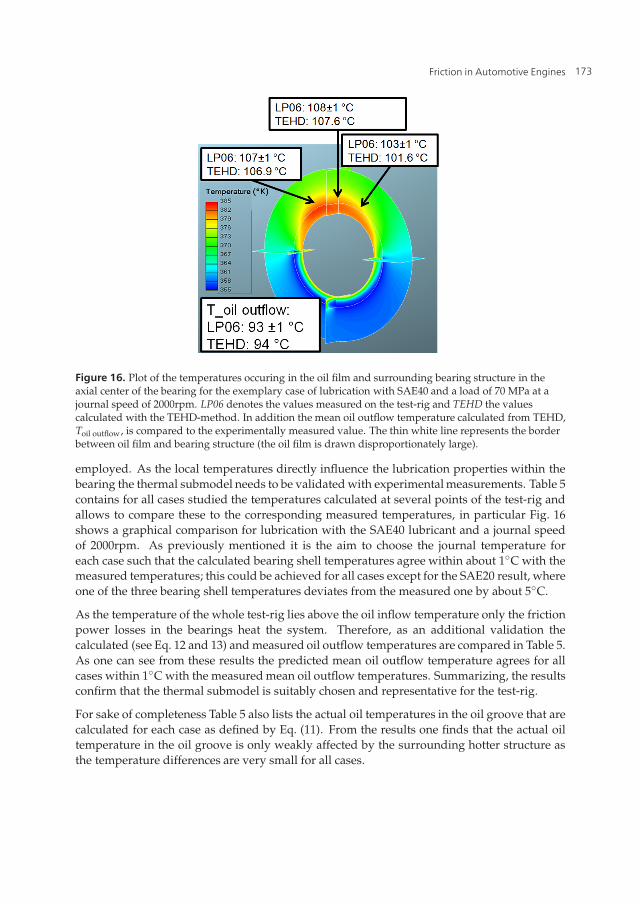
Figure 16. Plot of the temperatures occuring in the oil film and surrounding bearing structure in theaxial center of the bearing for the exemplary case of lubrication with SAE40 and a load of 70 MPa at ajournal speed of 2000rpm. LP06 denotes the values measured on the test-rig and TEHD the valuescalculated with the TEHD-method. In addition the mean oil outflow temperature calculated from TEHD,Toil outflow, is compared to the experimentally measured value. The thin white line represents the borderbetween oil film and bearing structure (the oil film is drawn disproportionately large).

employed. As the local temperatures directly influence the lubrication properties within thebearing the thermal submodel needs to be validated with experimental measurements. Table 5contains for all cases studied the temperatures calculated at several points of the test-rig andallows to compare these to the corresponding measured temperatures, in particular Fig. 16shows a graphical comparison for lubrication with the SAE40 lubricant and a journal speedof 2000rpm. As previously mentioned it is the aim to choose the journal temperature foreach case such that the calculated bearing shell temperatures agree within about 1◦C with themeasured temperatures; this could be achieved for all cases except for the SAE20 result, whereone of the three bearing shell temperatures deviates from the measured one by about 5◦C.

As the temperature of the whole test-rig lies above the oil inflow temperature only the frictionpower losses in the bearings heat the system. Therefore, as an additional validation thecalculated (see Eq. 12 and 13) and measured oil outflow temperatures are compared in Table 5.As one can see from these results the predicted mean oil outflow temperature agrees for allcases within 1◦C with the measured mean oil outflow temperatures. Summarizing, the resultsconfirm that the thermal submodel is suitably chosen and representative for the test-rig.

For sake of completeness Table 5 also lists the actual oil temperatures in the oil groove that arecalculated for each case as defined by Eq. (11). From the results one finds that the actual oiltemperature in the oil groove is only weakly affected by the surrounding hotter structure asthe temperature differences are very small for all cases.



3.2.5. Results for the friction power losses

In the following the results obtained with the various methods are discussed in terms offriction prediction; to this task the results from TEHD are compared to the results obtainedfrom EHD. As the TEHD comes with a largely increased cpu-time requirements, only thetest-bearing is investigated using TEHD in the following.

As briefly mentioned in Sec. 3.1, the discussed EHD-simulation model employs the samelubricant temperature for test and support bearings. This restriction needs to be removedfirst to allow consequently a detailed comparison of the results for the test-bearing obtainedfrom different simulation methods.

In [1] a new method is proposed that allows to easily calculate a suitable oil film temperaturefor the isothermal EHD-calculation. The procedure combines the measured bearing shelltemperature, TExp, and the supplied oil temperature, Toil supply, to

Tcomp = TExp − TExp − Toil supply

4(14)

and yields the same accurate results as can be seen in Figs. 17 and 18, but has the advantageof being applicable to single bearings. For reference also shown are the results that areobtained from the same EHD model but with the previously in Sec. 3.1 discussed temperatureestimation for all three combined bearings.

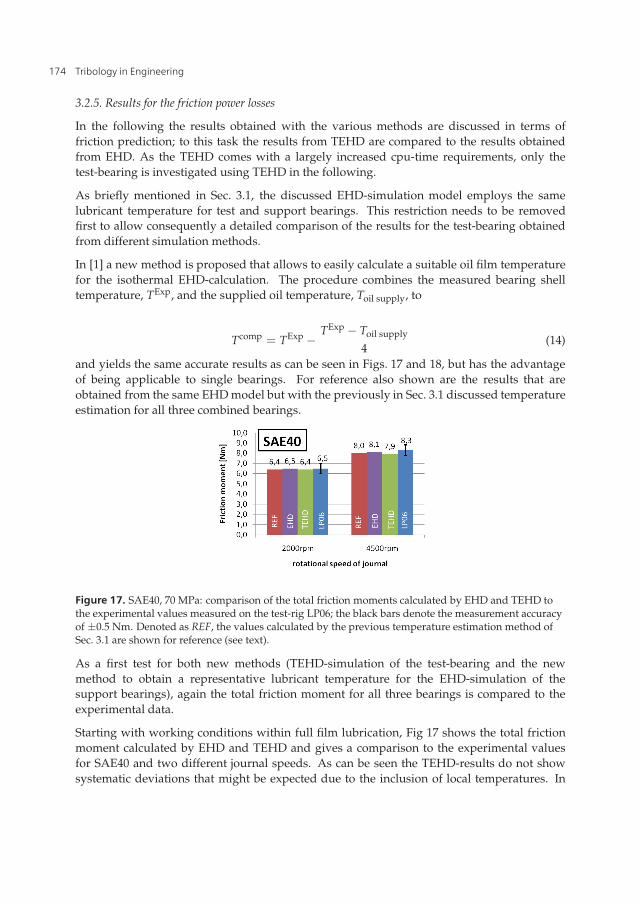
Figure 17. SAE40, 70 MPa: comparison of the total friction moments calculated by EHD and TEHD tothe experimental values measured on the test-rig LP06; the black bars denote the measurement accuracyof ±0.5 Nm. Denoted as REF, the values calculated by the previous temperature estimation method ofSec. 3.1 are shown for reference (see text).

As a first test for both new methods (TEHD-simulation of the test-bearing and the newmethod to obtain a representative lubricant temperature for the EHD-simulation of thesupport bearings), again the total friction moment for all three bearings is compared to theexperimental data.

Starting with working conditions within full film lubrication, Fig 17 shows the total frictionmoment calculated by EHD and TEHD and gives a comparison to the experimental valuesfor SAE40 and two different journal speeds. As can be seen the TEHD-results do not showsystematic deviations that might be expected due to the inclusion of local temperatures. In



fact, the results are almost identical; for a journal speed of 2000rpm 6.4 Nm are calculatedby TEHD in comparison to the 6.5 Nm predicted by EHD and the 6.5±0.4 Nm measured onthe test-rig. For an increased journal speed of 4500rpm the results are again very close with7.9 Nm and 8.1 Nm predicted by TEHD and EHD, respectively, compared to the 8.3±0.5 Nmmeasured experimentally.

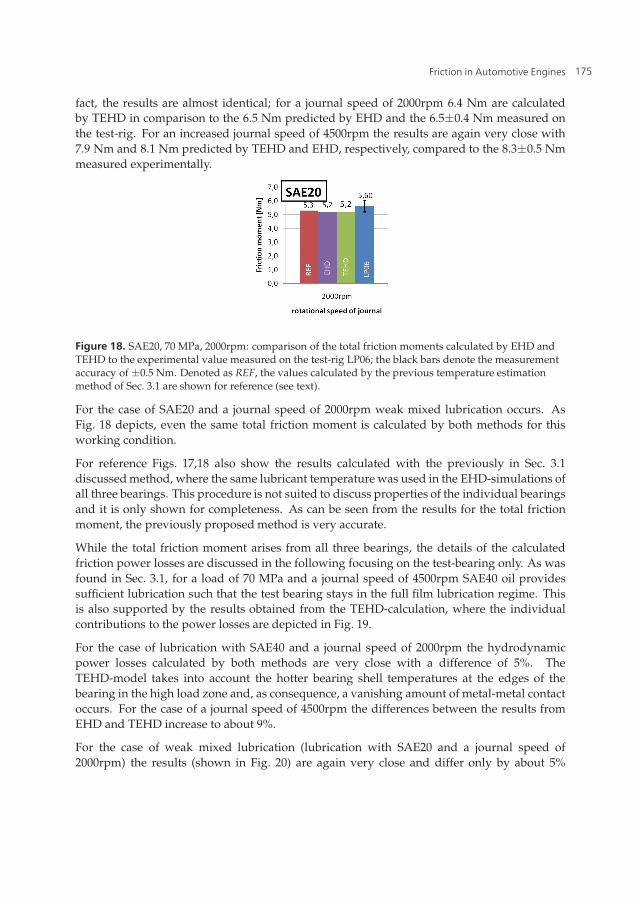
Figure 18. SAE20, 70 MPa, 2000rpm: comparison of the total friction moments calculated by EHD andTEHD to the experimental value measured on the test-rig LP06; the black bars denote the measurementaccuracy of ±0.5 Nm. Denoted as REF, the values calculated by the previous temperature estimationmethod of Sec. 3.1 are shown for reference (see text).

For the case of SAE20 and a journal speed of 2000rpm weak mixed lubrication occurs. AsFig. 18 depicts, even the same total friction moment is calculated by both methods for thisworking condition.

For reference Figs. 17,18 also show the results calculated with the previously in Sec. 3.1discussed method, where the same lubricant temperature was used in the EHD-simulations ofall three bearings. This procedure is not suited to discuss properties of the individual bearingsand it is only shown for completeness. As can be seen from the results for the total frictionmoment, the previously proposed method is very accurate.

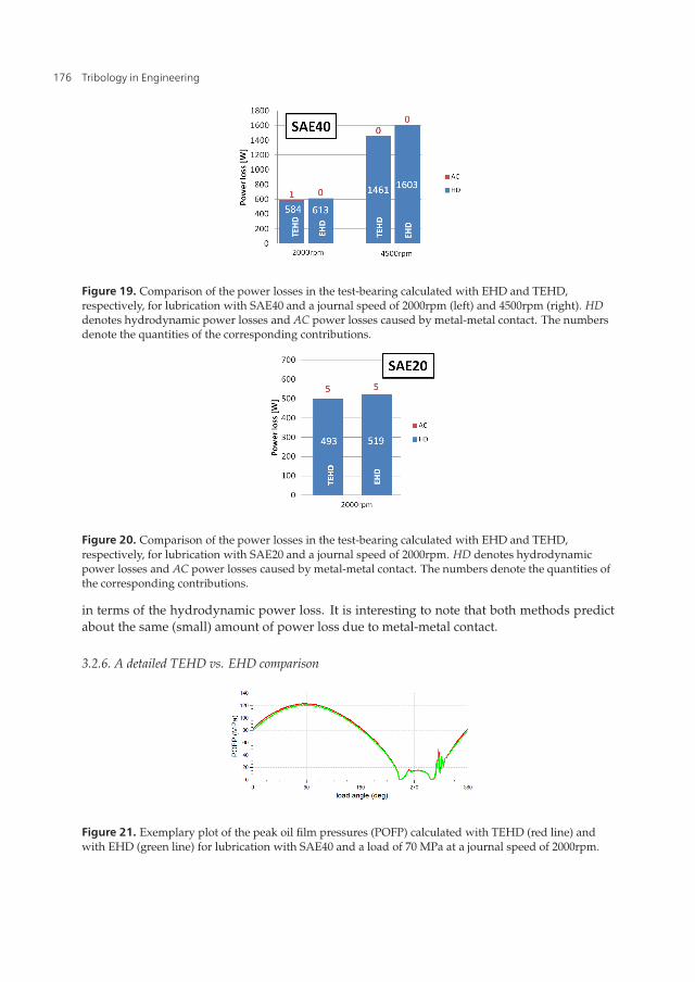
While the total friction moment arises from all three bearings, the details of the calculatedfriction power losses are discussed in the following focusing on the test-bearing only. As wasfound in Sec. 3.1, for a load of 70 MPa and a journal speed of 4500rpm SAE40 oil providessufficient lubrication such that the test bearing stays in the full film lubrication regime. Thisis also supported by the results obtained from the TEHD-calculation, where the individualcontributions to the power losses are depicted in Fig. 19.

For the case of lubrication with SAE40 and a journal speed of 2000rpm the hydrodynamicpower losses calculated by both methods are very close with a difference of 5%. TheTEHD-model takes into account the hotter bearing shell temperatures at the edges of thebearing in the high load zone and, as consequence, a vanishing amount of metal-metal contactoccurs. For the case of a journal speed of 4500rpm the differences between the results fromEHD and TEHD increase to about 9%.

For the case of weak mixed lubrication (lubrication with SAE20 and a journal speed of2000rpm) the results (shown in Fig. 20) are again very close and differ only by about 5%



Figure 19. Comparison of the power losses in the test-bearing calculated with EHD and TEHD,respectively, for lubrication with SAE40 and a journal speed of 2000rpm (left) and 4500rpm (right). HDdenotes hydrodynamic power losses and AC power losses caused by metal-metal contact. The numbersdenote the quantities of the corresponding contributions.

Figure 20. Comparison of the power losses in the test-bearing calculated with EHD and TEHD,respectively, for lubrication with SAE20 and a journal speed of 2000rpm. HD denotes hydrodynamicpower losses and AC power losses caused by metal-metal contact. The numbers denote the quantities ofthe corresponding contributions.

in terms of the hydrodynamic power loss. It is interesting to note that both methods predictabout the same (small) amount of power loss due to metal-metal contact.

3.2.6. A detailed TEHD vs. EHD comparison

Figure 21. Exemplary plot of the peak oil film pressures (POFP) calculated with TEHD (red line) andwith EHD (green line) for lubrication with SAE40 and a load of 70 MPa at a journal speed of 2000rpm.



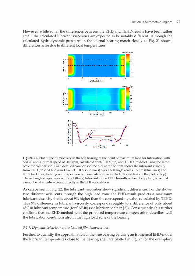
However, while so far the differences between the EHD and TEHD-results have been rathersmall, the calculated lubricant viscosities are expected to be notably different. Although thecalculated hydrodynamic pressures in the journal bearing match closely as Fig. 21 shows,differences arise due to different local temperatures.

Figure 22. Plot of the oil viscosity in the test bearing at the point of maximum load for lubrication withSAE40 and a journal speed of 2000rpm, calculated with EHD (top) and TEHD (middle) using the samescale for comparison. For a detailed comparison the plot at the bottom shows the lubricant viscosityfrom EHD (dashed lines) and from TEHD (solid lines) over shell angle across 8.5mm (blue lines) and0mm (red lines) bearing width (position of these cuts shown as black dashed lines in the plot on top).The rectangle shaped area with cool (thick) lubricant in the TEHD-results is the oil supply groove thatcannot be taken into account directly in the EHD-calculation.

As can be seen in Fig. 22, the lubricant viscosities show significant differences. For the showntwo different axial cuts through the high load zone the EHD-result predicts a maximumlubricant viscosity that is about 9% higher than the corresponding value calculated by TEHD.This 9% difference in lubricant viscosity corresponds roughly to a difference of only about4◦C in lubricant temperature (for SAE40) (see lubricant data in [3]). Consequently, this furtherconfirms that the EHD-method with the proposed temperature compensation describes wellthe lubrication conditions also in the high load zone of the bearing.

3.2.7. Dynamic behaviour of the local oil film temperatures

Further, to quantify the approximation of the true bearing by using an isothermal EHD-modelthe lubricant temperatures close to the bearing shell are plotted in Fig. 23 for the exemplary



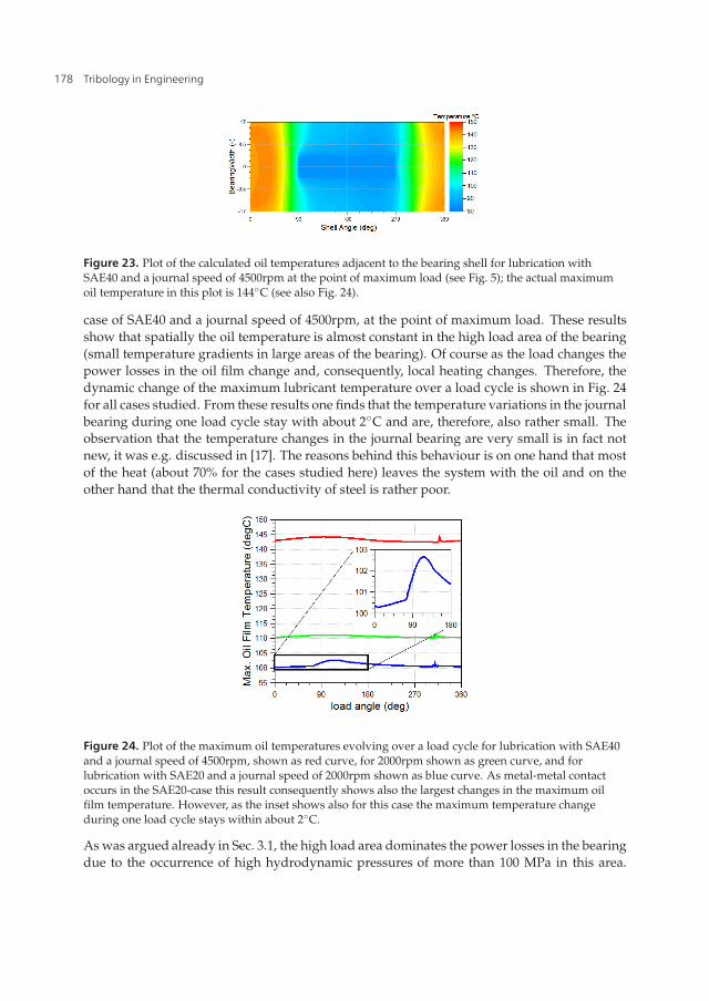
Figure 23. Plot of the calculated oil temperatures adjacent to the bearing shell for lubrication withSAE40 and a journal speed of 4500rpm at the point of maximum load (see Fig. 5); the actual maximumoil temperature in this plot is 144◦C (see also Fig. 24).

case of SAE40 and a journal speed of 4500rpm, at the point of maximum load. These resultsshow that spatially the oil temperature is almost constant in the high load area of the bearing(small temperature gradients in large areas of the bearing). Of course as the load changes thepower losses in the oil film change and, consequently, local heating changes. Therefore, thedynamic change of the maximum lubricant temperature over a load cycle is shown in Fig. 24for all cases studied. From these results one finds that the temperature variations in the journalbearing during one load cycle stay with about 2◦C and are, therefore, also rather small. Theobservation that the temperature changes in the journal bearing are very small is in fact notnew, it was e.g. discussed in [17]. The reasons behind this behaviour is on one hand that mostof the heat (about 70% for the cases studied here) leaves the system with the oil and on theother hand that the thermal conductivity of steel is rather poor.

Figure 24. Plot of the maximum oil temperatures evolving over a load cycle for lubrication with SAE40and a journal speed of 4500rpm, shown as red curve, for 2000rpm shown as green curve, and forlubrication with SAE20 and a journal speed of 2000rpm shown as blue curve. As metal-metal contactoccurs in the SAE20-case this result consequently shows also the largest changes in the maximum oilfilm temperature. However, as the inset shows also for this case the maximum temperature changeduring one load cycle stays within about 2◦C.

As was argued already in Sec. 3.1, the high load area dominates the power losses in the bearingdue to the occurrence of high hydrodynamic pressures of more than 100 MPa in this area.



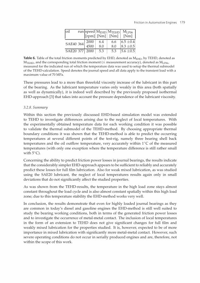
oil run speed MEHD MTEHD MLP06[rpm] [Nm] [Nm] [Nm]

SAE40 364 2000 6.4 6.6 6.5 ±0.44500 8.0 8.0 8.3 ±0.5

SAE20 377 2000 5.3 5.3 5.6 ±0.5

Table 6. Table of the total friction moments predicted by EHD, denoted as MEHD, by TEHD, denoted asMTEHD, and the corresponding total friction moment (±measurement accuracy), denoted as MLP06,measured for the indicated run of which the temperature data was used to setup the thermal submodelof the TEHD-calculation. Speed denotes the journal speed and all data apply to the transient load with amaximum value of 70 MPa.

These pressures lead to a more than threefold viscosity increase of the lubricant in this partof the bearing. As the lubricant temperature varies only weakly in this area (both spatiallyas well as dynamically), it is indeed well described by the previously proposed isothermalEHD-approach [3] that takes into account the pressure dependence of the lubricant viscosity.

3.2.8. Summary

Within this section the previously discussed EHD-based simulation model was extendedto TEHD to investigate differences arising due to the neglect of local temperatures. Withthe experimentally obtained temperature data for each working condition it was possibleto validate the thermal submodel of the TEHD-method. By choosing appropriate thermalboundary conditions it was shown that the TEHD-method is able to predict the occurringtemperatures at several different points of the test-rig, namely three bearing shell backtemperatures and the oil outflow temperature, very accurately within 1◦C of the measuredtemperatures (with only one exception where the temperature difference is still rather smallwith 5◦C).

Concerning the ability to predict friction power losses in journal bearings, the results indicatethat the considerably simpler EHD-approach appears to be sufficient to reliably and accuratelypredict these losses for full film lubrication. Also for weak mixed lubrication, as was studiedusing the SAE20 lubricant, the neglect of local temperatures results again only in smalldeviations that do not significantly affect the studied properties.

As was shown from the TEHD-results, the temperature in the high load zone stays almostconstant throughout the load cycle and is also almost constant spatially within this high loadzone; due to this temperature stability the EHD-method works very well.

In conclusion, the results demonstrate that even for highly loaded journal bearings as theyare common in today’s diesel and gasoline engines the EHD-method is still well suited tostudy the bearing working conditions, both in terms of the generated friction power lossesand to investigate the occurrence of metal-metal contact. The inclusion of local temperaturesin the form of an extension to TEHD does not give significant changes for full film andweakly mixed lubrication for the properties studied. It is, however, expected to be of moreimportance in mixed lubrication with significantly more metal-metal contact. However, suchsevere operating conditions do not occur in serially produced engines and are, therefore, notwithin the scope of this work.



4. Friction reduction for engines - a practical example

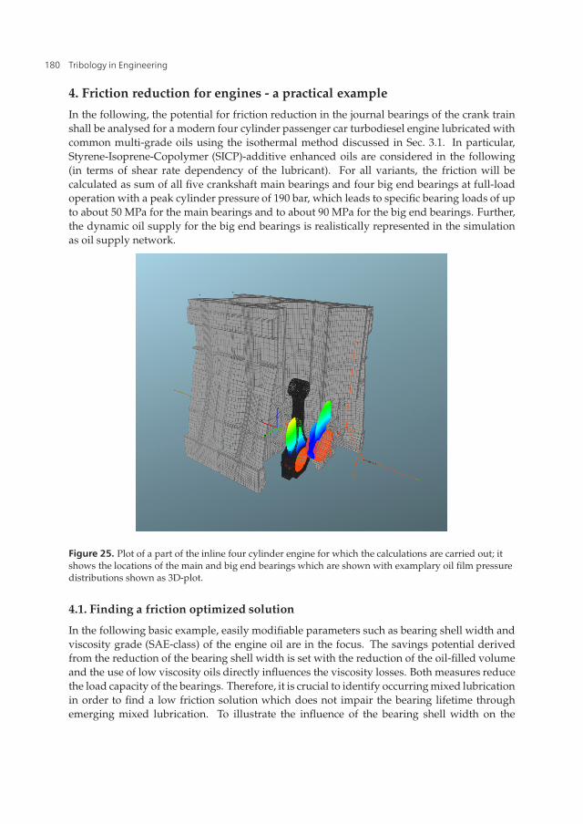
In the following, the potential for friction reduction in the journal bearings of the crank trainshall be analysed for a modern four cylinder passenger car turbodiesel engine lubricated withcommon multi-grade oils using the isothermal method discussed in Sec. 3.1. In particular,Styrene-Isoprene-Copolymer (SICP)-additive enhanced oils are considered in the following(in terms of shear rate dependency of the lubricant). For all variants, the friction will becalculated as sum of all five crankshaft main bearings and four big end bearings at full-loadoperation with a peak cylinder pressure of 190 bar, which leads to specific bearing loads of upto about 50 MPa for the main bearings and to about 90 MPa for the big end bearings. Further,the dynamic oil supply for the big end bearings is realistically represented in the simulationas oil supply network.

Figure 25. Plot of a part of the inline four cylinder engine for which the calculations are carried out; itshows the locations of the main and big end bearings which are shown with examplary oil film pressuredistributions shown as 3D-plot.

4.1. Finding a friction optimized solution

In the following basic example, easily modifiable parameters such as bearing shell width andviscosity grade (SAE-class) of the engine oil are in the focus. The savings potential derivedfrom the reduction of the bearing shell width is set with the reduction of the oil-filled volumeand the use of low viscosity oils directly influences the viscosity losses. Both measures reducethe load capacity of the bearings. Therefore, it is crucial to identify occurring mixed lubricationin order to find a low friction solution which does not impair the bearing lifetime throughemerging mixed lubrication. To illustrate the influence of the bearing shell width on the



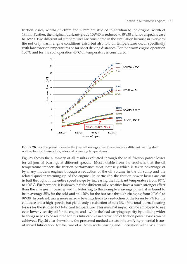
friction losses, widths of 21mm and 16mm are studied in addition to the original width of18mm. Further, the original lubricant-grade 10W40 is reduced to 0W30 and for a specific caseto 0W20. Two different oil temperatures are considered in the simulation because in everydaylife not only warm engine conditions exist, but also low oil temperatures occur specificallywith low exterior temperatures or for short driving distances. For the warm engine operation100◦C and for the cool operation 40◦C oil temperature is considered.

Figure 26. Friction power losses in the journal bearings at various speeds for different bearing shellwidths, lubricant viscosity grades and operating temperatures.

Fig. 26 shows the summary of all results evaluated through the total friction power lossesfor all journal bearings at different speeds. Most notable from the results is that the oiltemperature impacts the friction performance most intensely which is taken advantage ofby many modern engines through a reduction of the oil volume in the oil sump and therelated quicker warming-up of the engine. In particular, the friction power losses are cutin half throughout the entire speed range by increasing the lubricant temperature from 40◦Cto 100◦C. Furthermore, it is shown that the different oil viscosities have a much stronger effectthan the changes in bearing width. Referring to the example a savings potential is found tobe in average 35% for the cold and still 20% for the hot case through changing from 10W40 to0W30. In contrast, using more narrow bearings leads to a reduction of the losses by 9% for thecold case and a high speeds, but yields only a reduction of max 3% of the total journal bearinglosses for the studied hot lubricant temperature. This minimal impact can be employed to useeven lower viscosity oil for the engine and - while the load carrying capacity by utilizing widerbearings needs to be restored for this lubricant - a net reduction of friction power losses can beachieved. Fig. 26 also shows how the presented method assists in identifying potential issuesof mixed lubrication: for the case of a 16mm wide bearing and lubrication with 0W30 there



occurs for a lubricant temperature of 100◦C already significant metal-metal contact at 2000rpmwhich leads to a significant rise in friction for this engine and potentially to problems in theoperating reliability. However, with an enlarged bearing width even lower viscosity oil can beused; for the case presented the optimum is a low viscosity 0W20 oil combined with a broaderbearing shell, in this case 21mm. Thereby, in comparison to the original configuration with18mm bearings and 10W40 oil, the journal bearing losses can be reduced by 10% at 2000rpmand by approximately 30% at 4600rpm despite the significantly wider bearing shells.

4.2. Conclusion

The results show that small changes in the bearing geometry bear no significant impact onthe friction losses in the journal bearings. However, the use of a low viscosity lubricantholds obvious advantages in regards to a reduction of these losses, despite the need of widerbearings to retain the bearing load capacity. In the presented example this combination of lowviscosity lubricants with wider bearings revealed itself as optimal and proves approximately10-30% decreased losses in comparison to the initial situation. Alternatively, if more complexin design, the increase in size of the journal bearing diameter and the therefore necessarylarger journal diameter brings advantages also in regards to the NVH performance dueto the increased stiffness of the crankshaft. Further measures for friction reduction likean on-demand oil supply could potentially also attain significant savings and be analysedthrough the presented model.

While this basic example of friction reduction in engines displays the efficiency of variousmeasures, it is important to emphasise that the choice of the optimum lubricant affects thewhole engine and the other major source of mechanical losses, namely the piston assembly,challenges with (partly) opposing requirements to the lubricant. In this sense, the optimumchoice of the lubricant in terms of friction reduction shall only be taken under considerationof the complete system.

Acknowledgment

The authors would like to acknowledge several very interesting discussions on friction relatedtopics and want to express their gratitude in particular to C. Forstner (MIBA Bearing Group),F. Novotny-Farkas (OMV Refining & Marketing GmbH), A. Skiadas (K & S Gleitlager GmbH)and O. Knaus (AVL List GmbH).

Further, the authors acknowledge the kind permission of the MIBA Bearing Group andthe OMV Refining & Marketing GmbH to publish the results and the financial support ofthe ’COMET K2 - Competence Centers for Excellent Technologies Program’ of the AustrianFederal Ministry for Transport, Innovation and Technology (BMVIT), the Austrian FederalMinistry of Economy, Family and Youth (BMWFJ), the Austrian Research Promotion Agency(FFG), the Province of Styria and the Styrian Business Promotion Agency (SFG).

Author details

H. Allmaier, C. Priestner, D.E. Sander and F.M. ReichVirtual Vehicle Competence Center, Austria



5. References

[1] Allmaier, H., Priestner, C., Reich, F., Priebsch, H., Forstner, C. & Novotny-Farkas, F.[2012a]. Predicting friction reliably and accurately in journal bearings - extending thesimulation model to TEHD, Tribology International 58 (2013): 20-28.

[2] Allmaier, H., Priestner, C., Reich, F., Priebsch, H., Forstner, C. & Novotny-Farkas, F.[2012b]. Predicting friction reliably and accurately in journal bearings - the importanceof extensive oil-models, Tribology International 48: 93–101.

[3] Allmaier, H., Priestner, C., Six, C., Priebsch, H., Forstner, C. & Novotny-Farkas, F.[2011]. Predicting friction reliably and accurately in journal bearings–a systematicvalidation of simulation results with experimental measurements, Tribology International44(10): 1151–1160.

[4] Bair, S., Jarzynski, J. & Winer, W. [2001]. The temperature, pressure and time dependenceof lubricant viscosity, Tribology International 34(7): 461–468.

[5] Bukovnik, S., Offner, G., Caika, V., Priebsch, H. & Bartz, W. [2007].Thermo-elasto-hydrodynamic lubrication model for journal bearing including shearrate-dependent viscosity, Lubrication Science 19(4): 231–245.

[6] European Commission [2010]. Reducing CO2 emissions from passenger cars.URL: http://ec.europa.eu/clima/policies/transport/vehicles/cars/index_en.htm

[7] Fatu, A., Hajjam, M. & Bonneau, D. [2006]. A new model of thermoelastohydrodynamiclubrication in dynamically loaded journal bearings, Journal of tribology 128: 85.

[8] Fontaras, G. & Samaras, Z. [2010]. On the way to 130g CO2/km–estimating the futurecharacteristics of the average european passenger car, Energy Policy 38(4): 1826–1833.

[9] Greenwood, J. & Williamson, J. [1966]. Contact of nominally flat surfaces, Proceedings ofthe Royal Society of London. Series A, Mathematical and Physical Sciences 295: 300–319.

[10] Hall, D. & Moreland, J. [2001]. Fundamentals of rolling resistance, Rubber chemistry andtechnology 74: 525.

[11] Holmberg, K., Andersson, P. & Erdemir, A. [2012]. Global energy consumption due tofriction in passenger cars, Tribology International 47: 221–234.

[12] International Energy Agency [2006]. World energy outlook.[13] International Energy Agency [2008]. Worldwide trends in energy use and efficiency key

insights from IEA indicator analysis.[14] Kim, B. & Kim, K. [2001]. Thermo-elastohydrodynamic analysis of connecting rod

bearing in internal combustion engine, Journal of tribology 123: 444.[15] King, J. [2008]. The King review of low-carbon cars part I: the potential for reducing CO2

emissions from road transport, ISBN 978: 1–84532.[16] Körfer, T., Kolbeck, A., Schnorbus, T., Busch, H., Kinoo, B., Henning, L. & Severin, C.

[2011]. Fuel consumption potential of the passenger car diesel engine after EURO 6, 32.Internationales Wiener Motorensymposium, VDI, Vienna, Austria, pp. 99–122.

[17] Krasser, J. [1996]. Thermoelastohydrodynamische Analyse dynamisch belasteter Radialgleitlager(Thermoelastohydrodynamic analysis of dynamically loaded journal bearings), PhD thesis, GrazUniversity of Technology.

[18] Mittwollen, N. & Glienicke, J. [1990]. Operating conditions of multi-lobe journal bearingsunder high thermal loads, Journal of Tribology 112: 330.

[19] Mufti, R. & Priest, M. [2009]. Technique of simultaneous synchronized evaluationof the tribological components of an engine under realistic conditions, Proceedings



of the Institution of Mechanical Engineers, Part D: Journal of Automobile Engineering223(10): 1311–1325.

[20] Okamoto, Y., Kitahara, K., Ushijima, K., Aoyama, S., Xu, H. & Jones, G. [2000]. Astudy for wear and fatigue on engine bearings by using EHL analysis, JSAE Review21(2): 189–196.

[21] Patir, N. & Cheng, H. [1978]. An average flow model for determining effects ofthree-dimensional roughness on partial hydrodynamic lubrication, ASME, Transactions,Journal of Lubrication Technology 100: 12–17.

[22] Patir, N. & Cheng, H. [1979]. Application of average flow model to lubrication betweenrough sliding surfaces, ASME, Transactions, Journal of Lubrication Technology 101: 220–230.

[23] Priebsch, H. & Krasser, J. [1997]. Simulation of the oil film behaviour in elastic enginebearings considering pressure and temperature dependent oil viscosity, Tribology Series32: 651–659.

[24] Priestner, C., Allmaier, H., Priebsch, H. & Forstner, C. [2012]. Refined simulationof friction power loss in crank shaft slider bearings considering wear in the mixedlubrication regime, Tribology International 46(1): 200–207.

[25] Priestner, C., Allmaier, H., Reich, F., Forstner, C. & Novotny-Farkas, F. [2012]. Friction inhighly loaded journal bearings, MTZ 4: 310–315.

[26] Smith, R. [2008]. Enabling technologies for demand management: Transport, Energypolicy 36(12): 4444–4448.

[27] Tian, T. [2002]. Dynamic behaviours of piston rings and their practical impact. part 1:ring flutter and ring collapse and their effects on gas flow and oil transport, Proceedingsof the Institution of Mechanical Engineers, Part J: Journal of Engineering Tribology 216(4): 209.

[28] Wang, Y., Zhang, C., Wang, Q. & Lin, C. [2002]. A mixed-TEHD analysis andexperiment of journal bearings under severe operating conditions, Tribology international35(6): 395–407.

[29] Zhang, C. [2002]. TEHD behavior of non-newtonian dynamically loaded journal bearingsin mixed lubrication for direct problem, Journal of Tribology 124: 178.


Documents

Friction in Automotive Engines - InTech - OpenFriction in Automotive Engines 3 Figure 1. Friction measurement test-rig FRIDA during build-up at the Virtual Vehicle Competence Center