PNNL-13324

Frequency Modulation Spectroscopy Modeling for Remote Chemical Detection DM Sheen September 2000 Prepared for the U.S. Department of Energy under Contract DE-AC06-76RL01830

DISCLAIMER

This report was prepared as an account of work sponsored by an agency of the United States Government. Neither the United States Government nor any agency thereof, nor Battelle Memorial Institute, nor any of their employees, makes any warranty, express or implied, or assumes any legal liability or responsibility for the accuracy, completeness, or usefulness of any information, apparatus, product, or process disclosed, or represents that its use would not infringe privately owned rights. Reference herein to any specific commercial product, process, or service by trade name, trademark, manufacturer, or otherwise does not necessarily constitute or imply its endorsement, recommendation, or favoring by the United States Government or any agency thereof, or Battelle Memorial Institute. The views and opinions of authors expressed herein do not necessarily state or reflect those of the United States Government or any agency thereof.

PACIFIC NORTHWEST NATIONAL LABORATORY operated by BATTELLE

for the UNITED STATES DEPARTMENT OF ENERGY

under Contract DE-AC06-76RL01830

Printed in the United States of America

Available to DOE and DOE contractors from the Office of Scientific and Technical Information,

P.O. Box 62, Oak Ridge, TN 37831-0062; ph: (865) 576-8401 fax: (865) 576-5728

email: reports@adonis.osti.gov

Available to the public from the National Technical Information Service, U.S. Department of Commerce, 5285 Port Royal Rd., Springfield, VA 22161

ph: (800) 553-6847 fax: (703) 605-6900

email: orders@ntis.fedworld.gov online ordering: http://www.ntis.gov/ordering.htm

This document was printed on recycled paper. (8/00)

PNNL-13324

Frequency Modulation Spectroscopy Modeling for Remote Chemical Detection D. M. Sheen September 2000 Prepared for the U.S. Department of Energy under Contract DE-AC06-76RL01830 Pacific Northwest National Laboratory Richland, Washington 99352

iii

Summary Frequency modulation (FM) spectroscopy techniques show promise for active infrared remote chemical sensing because they have high immunity to optical noise, electronic noise, and various electronic and mechanical drifts. FM systems are responsive to sharp spectral features and can reduce the effects of spectral clutter due to interfering chemicals in the plume or in the atmosphere. The relatively high modulation frequencies used for FM also reduce the effects of albedo (reflectance) and plume variations. Conventional differential absorption lidar (DIAL) systems are performance limited by the noise induced by speckle. This report presents an analysis that shows FM-based sensors may significantly reduce the effects of speckle. This can result in reduced dwell times and faster area searches, as well as reducing various forms of spatial clutter. FM systems will require a laser system that is continuously tunable at relatively high frequencies (0.1 to 20 MHz). One promising candidate is the quantum-cascade (QC) laser (Capasso et al. 1999; Gmachl et al. 2000). The QC laser is potentially capable of power levels on the order of 1 Watt and frequency tuning on the order of 3 to 6 GHz, which is the performance level required for FM spectroscopy-based remote sensing. In this report, we describe a high-level numerical model for an FM spectroscopy-based remote sensing system, and application to two unmanned airborne vehicle (UAV) scenarios. A Predator scenario operating at a slant range of 6.5 km with a 10-cm-diameter telescope, and a Global Hawk scenario operating at a range of 30 km with a 20-cm-diameter telescope, have been assumed to allow estimation of the performance of potential FM systems. Numerical results obtained using the model show that the performance of both scenarios is limited to noise equivalent absorbances at the low 10-3 level. The detection sensitivity is limited by the effects of both detector noise and speckle. Sensitive heterodyne detection will be required to achieve that level of sensitivity using a 1 Watt per wavelength continuous-wave laser and assuming diffuse reflection from hard targets such as the ground. Diffuse reflection also induces speckle noise at the receiver. The speckle noise will also limit the performance of the system. However, analysis presented in this report shows that the FM spectroscopy based sensor may have reduced speckle noise relative to conventional DIAL systems. Both the receiver sensitivity limit and the speckle noise limit could be reduced dramatically by utilizing a retro-reflector or by using a ground-based receiver. However, these scenarios would require a more controlled environment which may not be acceptable. Obtaining the performance modeled in these scenarios will require the combination of heterodyne detection with significant speckle averaging. Efficient heterodyne detection of a highly speckled wavefront may require the development of coherent arrays. This technology would need to be developed for use in a remote infrared (IR) chemical detection system.

v

Contents Summary ............................................................................................................................................ iii 1.0 Introduction and Description of the Problem............................................................................. 1.1 2.0 Description of the FM Spectroscopy Model .............................................................................. 2.1 2.1 FM Signal Analysis ........................................................................................................... 2.2 2.1.1 Wavelength Modulation Analysis .......................................................................... 2.3 2.1.2 Frequency Modulation Analysis............................................................................. 2.4 2.1.3 Discussion............................................................................................................... 2.6 2.2 Laser and Optics Modeling................................................................................................ 2.6 2.3 Atmospheric Modeling ...................................................................................................... 2.7 2.3.1 Atmospheric Absorption......................................................................................... 2.7 2.3.2 Atmospheric Turbulence ........................................................................................ 2.7 2.4 Target Modeling ................................................................................................................ 2.10 2.4.1 Laser Radar Range Equation .................................................................................. 2.10 2.4.2 Speckle Modeling ................................................................................................... 2.11 2.5 Detector and Preamplifier Modeling ................................................................................. 2.17 2.5.1 Signal Current......................................................................................................... 2.17 2.5.2 Thermal Noise Current ........................................................................................... 2.18 2.5.3 Background Optical Flux and Detected Current..................................................... 2.18 2.5.4 Dark Current ........................................................................................................... 2.18 2.5.5 Shot Noise Components ......................................................................................... 2.19 2.6 Signal to Noise Ratio Analysis .......................................................................................... 2.19 3.0 Modeling Results ....................................................................................................................... 3.1 3.1 FM Spectral Signature Examples ...................................................................................... 3.1 3.2 UAV Scenarios .................................................................................................................. 3.4 3.3 Speckle Modeling Results ................................................................................................. 3.4 3.4 Predator Scenario SNR Modeling Results......................................................................... 3.9 3.5 Global Hawk Scenario SNR Modeling Results................................................................. 3.14 4.0 Modeling and Validation Issues and Conclusions ..................................................................... 4.1 4.1 Sensitivity .......................................................................................................................... 4.1 4.2 Target Induced Speckle ..................................................................................................... 4.1 4.3 Residual Amplitude Modulation........................................................................................ 4.2 4.4 Validation Experiments and Model Extensions ................................................................ 4.2 5.0 Acknowledgments...................................................................................................................... 5.1 6.0 References.................................................................................................................................. 6.1

vi

Figures 2.1 Block Diagram of the Modeled FM Spectroscopy-Based Chemical Detection System............ 2.1 2.2 Schematic Depiction of an FM Spectroscopy Trace Gas Detection System ............................. 2.2 2.3 Expected Platform Configuration .............................................................................................. 2.8 2.4 Remote Lidar Configuration and One-Dimensional Speckle Simulation Configuration .......... 2.13 2.5 Three-Dimensional Speckle Simulation Configuration ............................................................. 2.16 3.1 Optical Transmission Through the Atmosphere Using the FASCODE Simulation Software.... 3.1 3.2 FM Modeling Results for HCl ................................................................................................... 3.2 3.3 FM Modeling Results for SO2 ................................................................................................... 3.3 3.4 FM Modeling Results for HNO3................................................................................................ 3.3 3.5 One-Dimensional Speckle Modeling Results for Nυ = 0. .......................................................... 3.5 3.6 One-Dimensional Speckle Modeling Results for Nυ = 1 ........................................................... 3.6 3.7 One-Dimensional Speckle Modeling Results for Nυ = 50 ......................................................... 3.7 3.8 CNR and SNR Simulation Results Compared with Theoretical Formulas................................ 3.8 3.9 Lateral Speckle Simulations for the Predator and Global Hawk UAV Scenarios ..................... 3.8 3.10 Lateral Speckle Simulations for the Predator UAV Scenario..................................................... 3.9 3.11 Predator Scenario Noise Equivalent Absorbance (NEA) Versus Optical Power....................... 3.12 3.12 Predator Scenario Noise Equivalent Absorbance (NEA) Versus Range ................................... 3.12 3.13 Predator Scenario Noise Equivalent Absorbance (NEA) Versus Wavelength .......................... 3.13 3.14 Predator Scenario Noise Equivalent Absorbance (NEA) Versus Dwell Time .......................... 3.13 3.15 Global Hawk Scenario Noise Equivalent Absorbance (NEA) Versus Optical Power............... 3.16 3.16 Global Hawk Scenario Noise Equivalent Absorbance (NEA) Versus Range ........................... 3.16

vii

3.17 Global Hawk Scenario Noise Equivalent Absorbance (NEA) Versus Wavelength .................. 3.17 3.18 Global Hawk Scenario Noise Equivalent Absorbance (NEA) Versus Dwell Time .................. 3.17

Tables 2.1 Harmonic Amplitudes with Optimal Modulation Parameters for Gaussian and Lorentzian Line Shapes.............................................................................................................. 2.4 3.1 Predator UAV Operational Parameters...................................................................................... 3.4 3.2 Global Hawk UAV Operational Parameters.............................................................................. 3.4 3.3 Speckle Calculations for the Predator and Global Hawk UAV Scenarios................................. 3.9 3.4 Predator UAV Scenario Modeling Parameters .......................................................................... 3.10 3.5 Predator UAV Scenario SNR Modeling Results ....................................................................... 3.11 3.6 Global Hawk UAV Scenario Modeling Parameters .................................................................. 3.14 3.7 Global Hawk UAV Scenario Modeling Results ........................................................................ 3.15

1.1

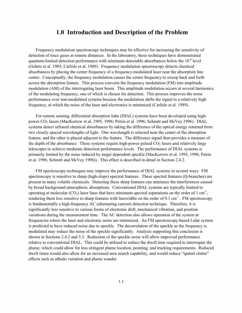
1.0 Introduction and Description of the Problem Frequency modulation spectroscopy techniques may be effective for increasing the sensitivity of detection of trace gases at remote distances. In the laboratory, these techniques have demonstrated quantum-limited detection performance with minimum detectable absorbances below the 10-6 level (Gehrtz et al. 1985; Carlisle et al. 1989). Frequency modulation spectroscopy detects chemical absorbances by placing the center frequency of a frequency-modulated laser near the absorption line center. Conceptually, the frequency modulation causes the center frequency to sweep back and forth across the absorption feature. This process converts the frequency modulation (FM) into amplitude modulation (AM) of the interrogating laser beam. This amplitude modulation occurs at several harmonics of the modulating frequency, one of which is chosen for detection. This process improves the noise performance over non-modulated systems because the modulation shifts the signal to a relatively high frequency, at which the noise of the laser and electronics is minimized (Carlisle et al. 1989). For remote sensing, differential absorption lidar (DIAL) systems have been developed using high-power CO2 lasers (MacKerrow et al. 1995, 1996; Petrin et al. 1996; Schmitt and McVey 1996). DIAL systems detect infrared chemical absorbances by taking the difference of the optical energy returned from two closely spaced wavelengths of light. One wavelength is selected near the center of the absorption feature, and the other is placed adjacent to the feature. The difference signal then provides a measure of the depth of the absorbance. These systems require high-power pulsed CO2 lasers and relatively large telescopes to achieve moderate detection performance levels. The performance of DIAL systems is primarily limited by the noise induced by target dependent speckle (MacKerrow et al. 1995, 1996; Petrin et al. 1996; Schmitt and McVey 1996)). This effect is described in detail in Section 2.4.2. FM spectroscopy techniques may improve the performance of DIAL systems in several ways. FM spectroscopy is sensitive to sharp (high-slope) spectral features. These spectral features (Q-branches) are present in many volatile chemicals. Detecting these sharp features can minimize the interferences caused by broad background atmospheric absorptions. Conventional DIAL systems are typically limited to operating at molecular (CO2) laser lines that have minimum spectral separations on the order of 1 cm-1, rendering them less sensitive to sharp features with linewidths on the order of 0.1 cm-1. FM spectroscopy is fundamentally a high-frequency AC (alternating current) detection technique. Therefore, it is significantly less sensitive to various forms of electronic drift, mechanical vibration, and position variations during the measurement time. The AC detection also allows operation of the system at frequencies where the laser and electronic noise are minimized. An FM spectroscopy-based Lidar system is predicted to have reduced noise due to speckle. The decorrelation of the speckle as the frequency is modulated may reduce the noise of the speckle significantly. Analysis supporting this conclusion is shown in Sections 2.4.2 and 3.3. Reduction of the speckle noise will allow improved performance relative to conventional DIAL. This could be utilized to reduce the dwell time required to interrogate the plume, which could allow for less stringent plume location, pointing, and tracking requirements. Reduced dwell times would also allow for an increased area search capability, and would reduce “spatial clutter” effects such as albedo variation and plume wander.

2.1

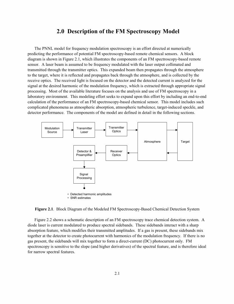
2.0 Description of the FM Spectroscopy Model The PNNL model for frequency modulation spectroscopy is an effort directed at numerically predicting the performance of potential FM spectroscopy-based remote chemical sensors. A block diagram is shown in Figure 2.1, which illustrates the components of an FM spectroscopy-based remote sensor. A laser beam is assumed to be frequency modulated with the laser output collimated and transmitted through the transmitter optics. This expanded beam then propagates through the atmosphere to the target, where it is reflected and propagates back through the atmosphere, and is collected by the receive optics. The received light is focused on the detector and the detected current is analyzed for the signal at the desired harmonic of the modulation frequency, which is extracted through appropriate signal processing. Most of the available literature focuses on the analysis and use of FM spectroscopy in a laboratory environment. This modeling effort seeks to expand upon this effort by including an end-to-end calculation of the performance of an FM spectroscopy-based chemical sensor. This model includes such complicated phenomena as atmospheric absorption, atmospheric turbulence, target-induced speckle, and detector performance. The components of the model are defined in detail in the following sections.

TransmitterLaser

Detector &Preamplifier

TransmitterOptics

ReceiverOptics

Atmosphere Target

Signal Processing

• Detected harmonic amplitudes• SNR estimates

ModulationSource

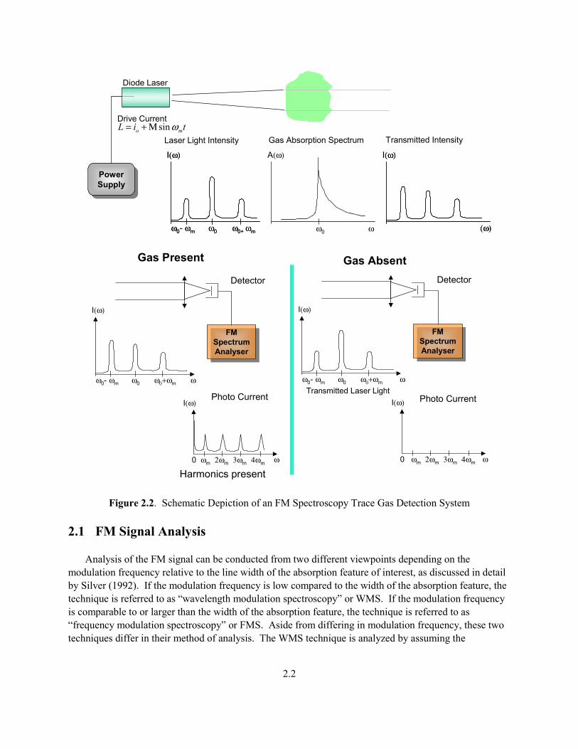
Figure 2.1. Block Diagram of the Modeled FM Spectroscopy-Based Chemical Detection System Figure 2.2 shows a schematic description of an FM spectroscopy trace chemical detection system. A diode laser is current modulated to produce spectral sidebands. These sidebands interact with a sharp absorption feature, which modifies their transmitted amplitudes. If a gas is present, these sidebands mix together at the detector to create photocurrent with harmonics of the modulation frequency. If there is no gas present, the sidebands will mix together to form a direct-current (DC) photocurrent only. FM spectroscopy is sensitive to the slope (and higher derivatives) of the spectral feature, and is therefore ideal for narrow spectral features.

2.2

I(ω)

ω0- ωm ω0 ω0+ ωm

I(ω)

ω0- ωm ω0 ω0+ ωm

I(ω)

(ω)

I(ω)

(ω)

A(ω)

ω0 ω

Laser Light Intensity Gas Absorption Spectrum Transmitted Intensity

PowerSupplyPowerSupply

Diode Laser

Drive CurrenttiL mo ωsinΜ+=

Gas Present

Detector

Photo CurrentI(ω)

0 ωm 2ωm 3ωm 4ωm

FMSpectrumAnalyser

FMSpectrumAnalyser

Harmonics present

I(ω)

ω0- ωm ω0 ω0+ωm ω

Gas AbsentDetector

Photo CurrentI(ω)

0 ωm 2ωm 3ωm 4ωm

FMSpectrumAnalyser

FMSpectrumAnalyser

I(ω)

ω0- ωm ω0 ω0+ωm ωTransmitted Laser Light

ω ω

Figure 2.2. Schematic Depiction of an FM Spectroscopy Trace Gas Detection System 2.1 FM Signal Analysis Analysis of the FM signal can be conducted from two different viewpoints depending on the modulation frequency relative to the line width of the absorption feature of interest, as discussed in detail by Silver (1992). If the modulation frequency is low compared to the width of the absorption feature, the technique is referred to as “wavelength modulation spectroscopy” or WMS. If the modulation frequency is comparable to or larger than the width of the absorption feature, the technique is referred to as “frequency modulation spectroscopy” or FMS. Aside from differing in modulation frequency, these two techniques differ in their method of analysis. The WMS technique is analyzed by assuming the

2.3

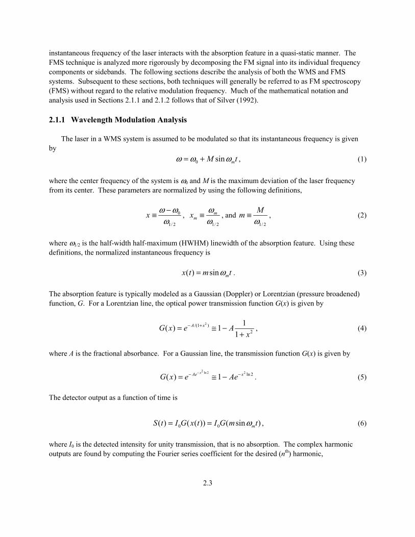
instantaneous frequency of the laser interacts with the absorption feature in a quasi-static manner. The FMS technique is analyzed more rigorously by decomposing the FM signal into its individual frequency components or sidebands. The following sections describe the analysis of both the WMS and FMS systems. Subsequent to these sections, both techniques will generally be referred to as FM spectroscopy (FMS) without regard to the relative modulation frequency. Much of the mathematical notation and analysis used in Sections 2.1.1 and 2.1.2 follows that of Silver (1992). 2.1.1 Wavelength Modulation Analysis The laser in a WMS system is assumed to be modulated so that its instantaneous frequency is given by 0 sin mM tω ω ω= + , (1) where the center frequency of the system is ω0 and M is the maximum deviation of the laser frequency from its center. These parameters are normalized by using the following definitions,

0

1/ 2

x ω ωω−≡ ,

1/ 2

mmx ω

ω≡ , and

1/ 2

Mmω

≡ , (2)

where ω1/2 is the half-width half-maximum (HWHM) linewidth of the absorption feature. Using these definitions, the normalized instantaneous frequency is ( ) sin mx t m tω= . (3) The absorption feature is typically modeled as a Gaussian (Doppler) or Lorentzian (pressure broadened) function, G. For a Lorentzian line, the optical power transmission function G(x) is given by

2/(1 )

2

1( ) 11

A xG x e Ax

− += ≅ −+

, (4)

where A is the fractional absorbance. For a Gaussian line, the transmission function G(x) is given by

2 ln 2 2 ln 2( ) 1

xAe xG x e Ae−− −= ≅ − . (5)

The detector output as a function of time is

0 0( ) ( ( )) ( sin )mS t I G x t I G m tω= = , (6) where I0 is the detected intensity for unity transmission, that is no absorption. The complex harmonic outputs are found by computing the Fourier series coefficient for the desired (nth) harmonic,

2.4

0 0

1 ( )T

nI S t dtT= = ∫

0

2 ( ) mT jn t

nI S t e dtT

ω= ∫ , (7)

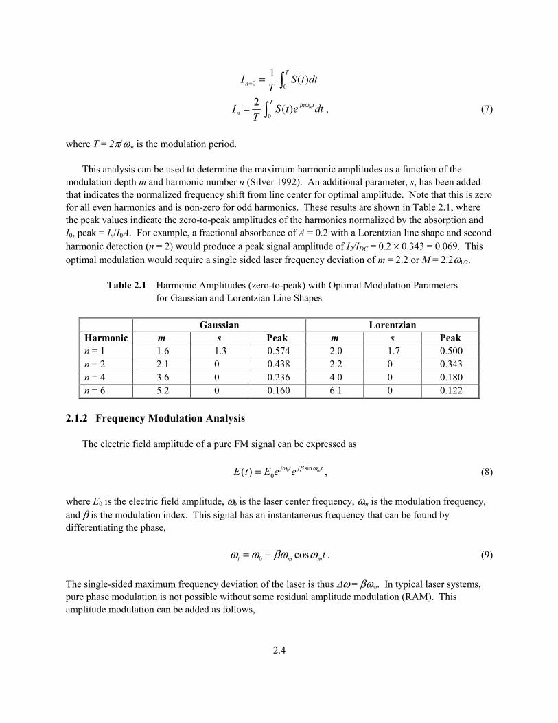
where T = 2π/ωm is the modulation period. This analysis can be used to determine the maximum harmonic amplitudes as a function of the modulation depth m and harmonic number n (Silver 1992). An additional parameter, s, has been added that indicates the normalized frequency shift from line center for optimal amplitude. Note that this is zero for all even harmonics and is non-zero for odd harmonics. These results are shown in Table 2.1, where the peak values indicate the zero-to-peak amplitudes of the harmonics normalized by the absorption and I0, peak = In/I0A. For example, a fractional absorbance of A = 0.2 with a Lorentzian line shape and second harmonic detection (n = 2) would produce a peak signal amplitude of I2/IDC = 0.2 × 0.343 = 0.069. This optimal modulation would require a single sided laser frequency deviation of m = 2.2 or M = 2.2ω1/2. Table 2.1. Harmonic Amplitudes (zero-to-peak) with Optimal Modulation Parameters

for Gaussian and Lorentzian Line Shapes

Gaussian Lorentzian Harmonic m s Peak m s Peak n = 1 1.6 1.3 0.574 2.0 1.7 0.500 n = 2 2.1 0 0.438 2.2 0 0.343 n = 4 3.6 0 0.236 4.0 0 0.180 n = 6 5.2 0 0.160 6.1 0 0.122

2.1.2 Frequency Modulation Analysis The electric field amplitude of a pure FM signal can be expressed as 0 sin

0( ) mj t j tE t E e eω β ω= , (8) where E0 is the electric field amplitude, ω0 is the laser center frequency, ωm is the modulation frequency, and β is the modulation index. This signal has an instantaneous frequency that can be found by differentiating the phase, 0 cosi m mtω ω βω ω= + . (9) The single-sided maximum frequency deviation of the laser is thus ∆ω = βωm. In typical laser systems, pure phase modulation is not possible without some residual amplitude modulation (RAM). This amplitude modulation can be added as follows,

2.5

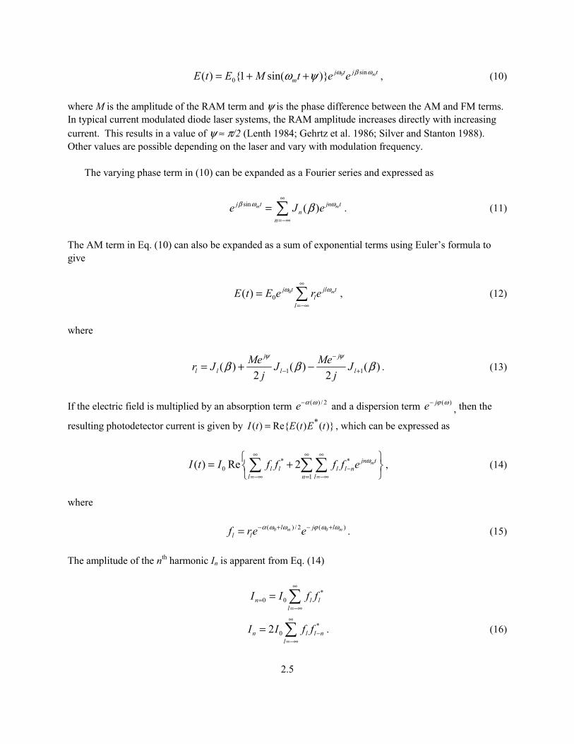
0 sin0( ) 1 sin( ) mj t j t

mE t E M t e eω β ωω ψ= + + , (10) where M is the amplitude of the RAM term and ψ is the phase difference between the AM and FM terms. In typical current modulated diode laser systems, the RAM amplitude increases directly with increasing current. This results in a value of ψ ≈ π/2 (Lenth 1984; Gehrtz et al. 1986; Silver and Stanton 1988). Other values are possible depending on the laser and vary with modulation frequency. The varying phase term in (10) can be expanded as a Fourier series and expressed as

sin ( )m mj t jn tn

ne J eβ ω ωβ

∞

=−∞

= ∑ . (11)

The AM term in Eq. (10) can also be expanded as a sum of exponential terms using Euler’s formula to give

00( ) mj t jl t

ll

E t E e reω ω∞

=−∞

= ∑ , (12)

where

1 1( ) ( ) ( )2 2

j j

l l l lMe Mer J J J

j j

ψ ψ

β β β−

− += + − . (13)

If the electric field is multiplied by an absorption term ( ) / 2e α ω− and a dispersion term ( )je ϕ ω−

, then the

resulting photodetector current is given by )()(Re)( * tEtEtI = , which can be expressed as

* *0

1

( ) Re 2 mjn tl l l l n

l n l

I t I f f f f e ω∞ ∞ ∞

−=−∞ = =−∞

= + ∑ ∑∑ , (14)

where 0 0( ) / 2 ( )m ml j l

l lf re eα ω ω ϕ ω ω− + − += . (15) The amplitude of the nth harmonic In is apparent from Eq. (14)

*0 0n l l

lI I f f

∞

==−∞

= ∑

*02n l l n

lI I f f

∞

−=−∞

= ∑ . (16)

2.6

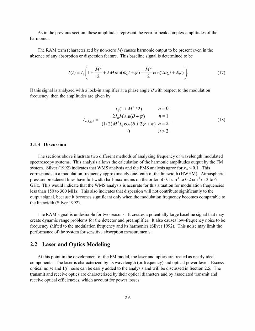
As in the previous section, these amplitudes represent the zero-to-peak complex amplitudes of the harmonics. The RAM term (characterized by non-zero M) causes harmonic output to be present even in the absence of any absorption or dispersion feature. This baseline signal is determined to be

2 2

0( ) 1 2 sin( ) cos(2 2 )2 2m m

M MI t I M t tω ψ ω ψ = + + + − +

. (17)

If this signal is analyzed with a lock-in amplifier at a phase angle θ with respect to the modulation frequency, then the amplitudes are given by

20

0, 2

0

0(1 / 2)12 sin( )2(1/ 2) cos( 2 )20

n RAM

nI MnI M

InM In

θ ψθ ψ π

=+=+

==+ +>

. (18)

2.1.3 Discussion The sections above illustrate two different methods of analyzing frequency or wavelength modulated spectroscopy systems. This analysis allows the calculation of the harmonic amplitudes output by the FM system. Silver (1992) indicates that WMS analysis and the FMS analysis agree for xm < 0.1. This corresponds to a modulation frequency approximately one-tenth of the linewidth (HWHM). Atmospheric pressure broadened lines have full-width half-maximums on the order of 0.1 cm-1 to 0.2 cm-1 or 3 to 6 GHz. This would indicate that the WMS analysis is accurate for this situation for modulation frequencies less than 150 to 300 MHz. This also indicates that dispersion will not contribute significantly to the output signal, because it becomes significant only when the modulation frequency becomes comparable to the linewidth (Silver 1992). The RAM signal is undesirable for two reasons. It creates a potentially large baseline signal that may create dynamic range problems for the detector and preamplifier. It also causes low-frequency noise to be frequency shifted to the modulation frequency and its harmonics (Silver 1992). This noise may limit the performance of the system for sensitive absorption measurements. 2.2 Laser and Optics Modeling At this point in the development of the FM model, the laser and optics are treated as nearly ideal components. The laser is characterized by its wavelength (or frequency) and optical power level. Excess optical noise and 1/f noise can be easily added to the analysis and will be discussed in Section 2.5. The transmit and receive optics are characterized by their optical diameters and by associated transmit and receive optical efficiencies, which account for power losses.

2.7

2.3 Atmospheric Modeling Remote chemical sensing will require laser beam propagation through at least several kilometers of the atmosphere. The atmosphere is expected to impact the system primarily through atmospheric absorption and turbulence effects. 2.3.1 Atmospheric Absorption Atmospheric absorption is modeled using a version of FASCODE, that is commercially distributed by the Ontar Corporation. FASCODE makes use of the HITRAN database, which is a line-by-line database of the molecules typically found in the atmosphere. FASCODE uses a layered model to account for variation of the molecular concentration, temperature, and pressure with altitude. Information about Ontar is available at their web site at http://www.ontar.com/. Information about HITRAN is available at http://ww.hitran.com/. Example modeling calculations using the output of this software are presented in Section 3.1. 2.3.2 Atmospheric Turbulence Turbulence in the atmosphere affects the propagation of the laser beam primarily by creating small variations in the local index of refraction. These variations are characterized by the atmospheric structure coefficient, 2

nC , and cause a number of optical effects including additional beam spreading, beam wander, finite transverse coherence length, and scintillation (Beland 1993; Miller and Friedman 1996; Andrews and Phillips 1998).

2.3.2.1 Structure Coefficient Turbulence-induced index of refraction variations are characterized by the index of refraction structure coefficient 2

nC (units are m-2/3). The structure coefficient typically is near the ground and becomes insignificant at high altitudes (Beland 1993; Tyson and Ulrich 1993; Miller and Friedman 1996; Tyson 1998). A simple model for 2

nC for horizontal paths near the ground is given by (Miller and Friedman 1996) 2 142 10nC −= × (day)

2 1410nC −= (night). (19) A more detailed model is the Hufnagel-Valley model for 2

nC accounts for the variation with altitude and is given by (Miller and Friedman 1996)

2.8

102 26 2 /1000 16 /1500 14 /100( ) 8.2 10 2.7 10 1.7 10

1000h h h

nhC h W e e e− − − − − − = × + × + ×

, (20)

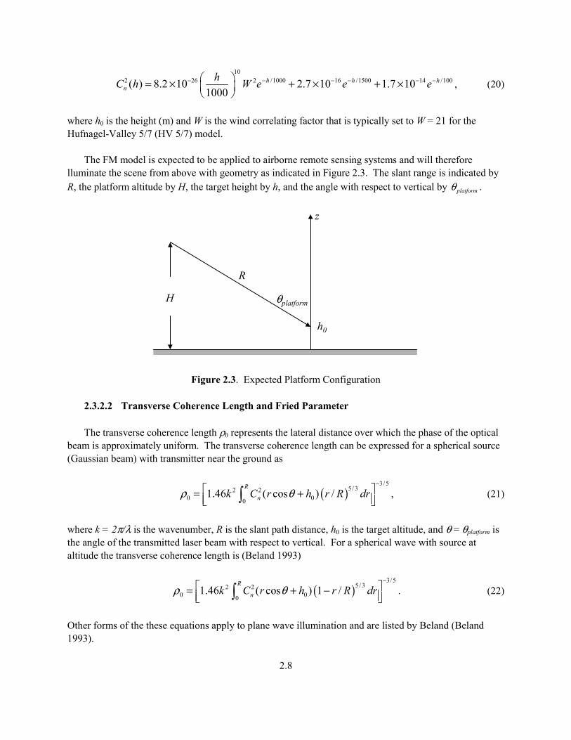
where h0 is the height (m) and W is the wind correlating factor that is typically set to W = 21 for the Hufnagel-Valley 5/7 (HV 5/7) model. The FM model is expected to be applied to airborne remote sensing systems and will therefore lluminate the scene from above with geometry as indicated in Figure 2.3. The slant range is indicated by R, the platform altitude by H, the target height by h, and the angle with respect to vertical by platformθ .

H

h0

R

z

θplatform

Figure 2.3. Expected Platform Configuration

2.3.2.2 Transverse Coherence Length and Fried Parameter The transverse coherence length ρ0 represents the lateral distance over which the phase of the optical beam is approximately uniform. The transverse coherence length can be expressed for a spherical source (Gaussian beam) with transmitter near the ground as

( )3/5

5/ 32 20 00

1.46 ( cos ) /R

nk C r h r R drρ θ−

= + ∫ , (21)

where k = 2π/λ is the wavenumber, R is the slant path distance, h0 is the target altitude, and θ = θplatform is the angle of the transmitted laser beam with respect to vertical. For a spherical wave with source at altitude the transverse coherence length is (Beland 1993)

( )3/5

5/ 32 20 00

1.46 ( cos ) 1 /R

nk C r h r R drρ θ−

= + − ∫ . (22)

Other forms of the these equations apply to plane wave illumination and are listed by Beland (Beland 1993).

2.9

The Fried parameter 0r is a similar measure of the lateral coherence length and is given by 0 02.1r ρ= . (23)

2.3.2.3 Beam Spreading and Wander The transmitted beam diameter is affected by the normal diffraction process, as well as by turbulence effects. The transmitted spot diameter is given by 2tar LD ρ= , (24) where ρL is the long-term average beam radius. The average beam radius is given by the quadrature sum of the diffraction radius ρd, the short-term turbulence induced radius ρs, and longer-term centroid wander caused by turbulence ρc as (Fante 1975; Beland 1993) 2 2 2 2

L d s cρ ρ ρ ρ= + + . (25) The radii are defined as

22 2

22 2

4 14d

R D Rk D F

ρ = + −

, (26)

2

02 20

2 6 /512 3

002 2

0

4 2

4 1 0.62 2s

R Dk

R Dk D

ρρ

ρρ ρ

ρ

≤

= − >

, (27)

and

0

2 2

02 5/ 3 1/ 30

0 22.97 2c

DR D

k D

ρρ

ρρ

≤= >

, (28)

where D is the effective transmitter diameter, R is the range, ρ0 is the transverse coherence length, k = 2π/λ is the wavenumber, and –F is the radius of curvature of the beam at the transmitter aperture.

2.3.2.4 Scintillation

2.10

Scintillation is the variance of the optical power caused by turbulence and can be expressed

2

242

2

( )1I

I Ie

Iχσσ

−= = − , (29)

where 2

Iσ is the scintillation index and 2xσ is the log amplitude variance. The log amplitude variance has

different formulations depending on the type of source (spherical or plane wave) and the source location (source at altitude or source at ground level) (Beland 1993). A Gaussian beam will approximately follow the spherical wave source formulation. For a spherical wave source at ground level,

5/ 6

2 7 / 6 2 5/ 60

0

0.56 ( cos )( )R

nrk C r h R r drRχσ θ = + −

⌠⌡

. (30)

For a spherical wave source at altitude looking down,

5/ 6

2 7 / 6 2 5/ 60

0

0.56 ( cos ) ( )R

nR rk C r h r dr

Rχσ θ − = +

⌠⌡

. (31)

2.4 Target Modeling Remote chemical sensing in uncontrolled environments may need to rely on diffuse (optically rough surface) reflection to return the probing laser beam signal to the receiver. In more controlled environments, a retro-reflector, or bi-static operation may be used to enhance the performance of the system. A laser radar approach can be used to model the returned optical power. For diffuse targets, the effects of target-induced speckle can be very significant and are examined in Section 2.4.2. 2.4.1 Laser Radar Range Equation A laser radar range equation formalism is used to model the returned power for all three of the above mentioned scenarios. The returned power from the target is given by (Kamerman 1993),

2

1 22 2/ 4 4 4

T A t A C rR

tar

P KT T DPD r

η π ηπ π

= Γ (W), (32)

where PT is the transmitted power, K is the beam profile function (equal to one for uniform beam), TA1 is the atmospheric transmission from source to target, TA2 is the atmospheric transmission from target to

2.11

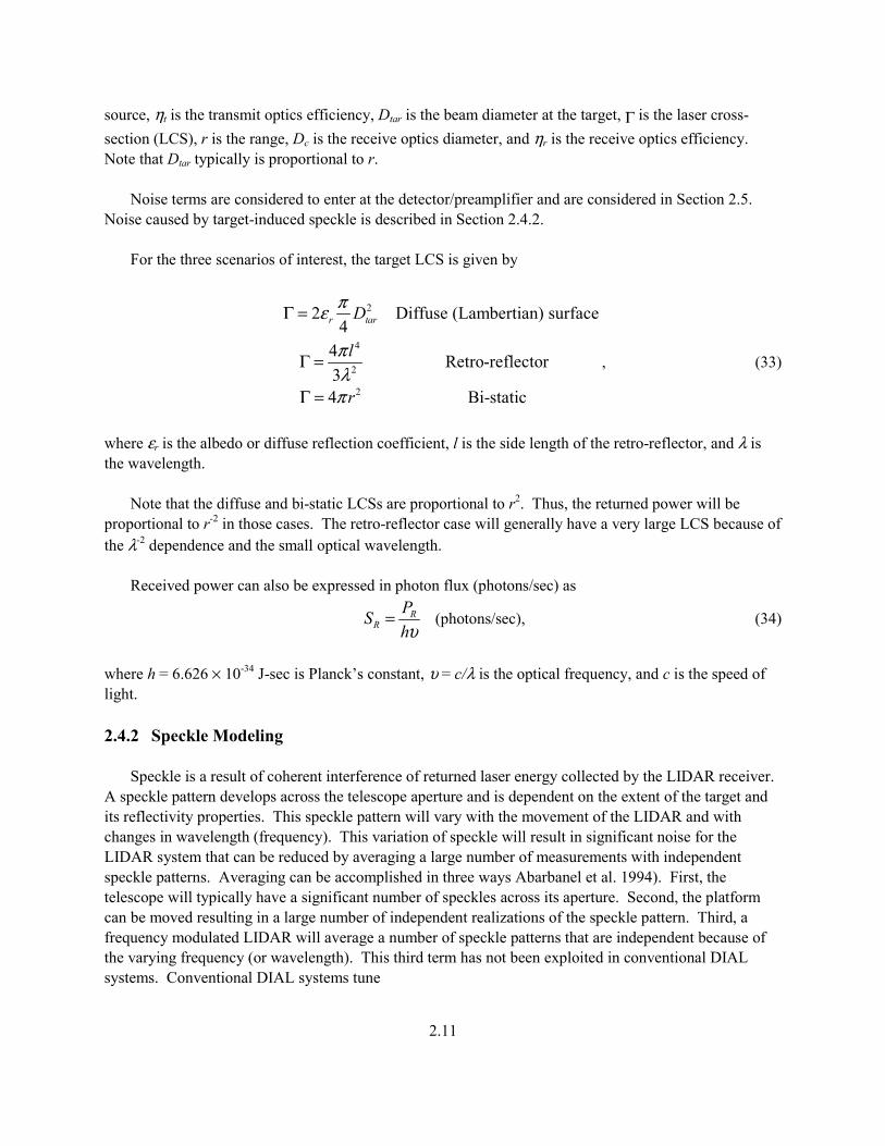
source, ηt is the transmit optics efficiency, Dtar is the beam diameter at the target, Γ is the laser cross-section (LCS), r is the range, Dc is the receive optics diameter, and ηr is the receive optics efficiency. Note that Dtar typically is proportional to r. Noise terms are considered to enter at the detector/preamplifier and are considered in Section 2.5. Noise caused by target-induced speckle is described in Section 2.4.2. For the three scenarios of interest, the target LCS is given by

2

4

2

2

2 Diffuse (Lambertian) surface4

4 Retro-reflector34 Bi-static

r tarD

l

r

πε

πλπ

Γ =

Γ =

Γ =

, (33)

where εr is the albedo or diffuse reflection coefficient, l is the side length of the retro-reflector, and λ is the wavelength. Note that the diffuse and bi-static LCSs are proportional to r2. Thus, the returned power will be proportional to r-2 in those cases. The retro-reflector case will generally have a very large LCS because of the λ-2 dependence and the small optical wavelength. Received power can also be expressed in photon flux (photons/sec) as

RR

PShυ

= (photons/sec), (34)

where h = 6.626 × 10-34 J-sec is Planck’s constant, υ = c/λ is the optical frequency, and c is the speed of light. 2.4.2 Speckle Modeling Speckle is a result of coherent interference of returned laser energy collected by the LIDAR receiver. A speckle pattern develops across the telescope aperture and is dependent on the extent of the target and its reflectivity properties. This speckle pattern will vary with the movement of the LIDAR and with changes in wavelength (frequency). This variation of speckle will result in significant noise for the LIDAR system that can be reduced by averaging a large number of measurements with independent speckle patterns. Averaging can be accomplished in three ways Abarbanel et al. 1994). First, the telescope will typically have a significant number of speckles across its aperture. Second, the platform can be moved resulting in a large number of independent realizations of the speckle pattern. Third, a frequency modulated LIDAR will average a number of speckle patterns that are independent because of the varying frequency (or wavelength). This third term has not been exploited in conventional DIAL systems. Conventional DIAL systems tune

2.12

the laser to only two discrete wavelengths to make the differential absorption measurement and are unable to average all of the independent realizations of the speckle over the frequency range between the two wavelengths. For a single point target or retro-reflector and with no absorption, a perfectly frequency modulated signal given by Eq. (8) has a constant amplitude .|||)(|)( 0

20

2 IEtEtI ≡== Modifying Eqs. (12) and (13) by assuming no RAM (M = 0) and allowing for frequency-dependent absorption and round-trip propagation to a target results in

0 ( ) / 2 20( ) ( ) mj t jn tj kz

nn

E t E e J e e eω ωα ωβ γ∞

− −

=−∞

= ∑ , (35)

where γ is the reflectivity of the target, k = ω/c is the wavenumber, z is the distance to the target, and

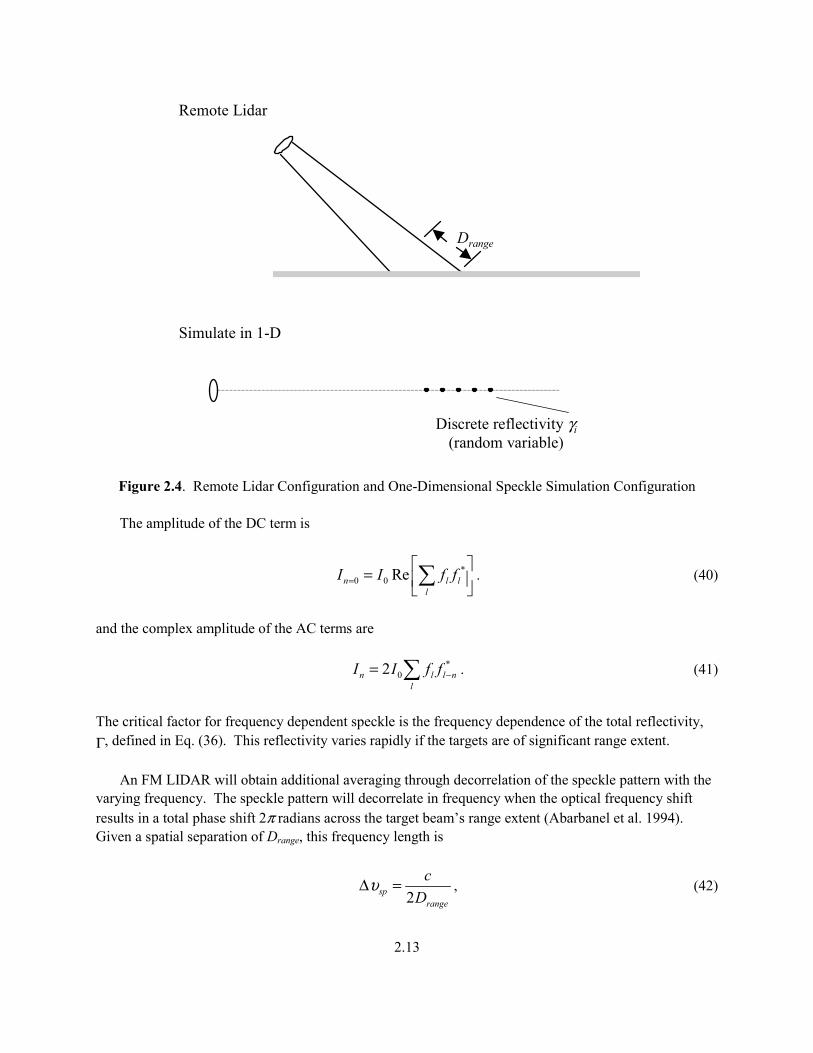
2/)(ωα−e is the attenuation term. The frequency ω is evaluated only at the discrete harmonics of ωm, i.e., ω = ω0 + nωm. Allowing for numerous scattering targets of total spatial extent Drange as shown in Figure 2.4 results in

0 02( )( ) / 20

1

( ) ( )refl

m m i

n

n

Nj t jn t j k nk z

n in i

E t E e J e e eω ωα ω

α

β γ∞

− +−

=−∞ =

Γ

=

∑ ∑ , (36)

where k0 ≡ ω0/c and km ≡ ωm/c. Simplifying using the definitions shown in Eq. (36) results in

00( ) ( ) mj t jn t

n n nn

E t E e J eω ωβ α∞

=−∞

= Γ∑ . (37)

For additional simplicity, define f1 = J1(β)αlΓ1 and Eq. (37) can be re-written as

00( ) mj t jl t

ll

E t E e f eω ω∞

=−∞

= ∑ . (38)

The output of the detector is proportional to

*

* *0

1

( ) Re[ ( ) ( )]

Re 2 mjn tl l l l n

l n l

I t E t E t

I f f f f e ω∞ ∞ ∞

−=−∞ = =−∞

=

= + ∑ ∑∑

. (39)

2.13

Remote Lidar

Drange

Simulate in 1-D

Discrete reflectivity γi(random variable)

Figure 2.4. Remote Lidar Configuration and One-Dimensional Speckle Simulation Configuration The amplitude of the DC term is

*0 0 Ren l l

lI I f f=

= ∑ . (40)

and the complex amplitude of the AC terms are *

02n l l nl

I I f f −= ∑ . (41)

The critical factor for frequency dependent speckle is the frequency dependence of the total reflectivity, Γ, defined in Eq. (36). This reflectivity varies rapidly if the targets are of significant range extent. An FM LIDAR will obtain additional averaging through decorrelation of the speckle pattern with the varying frequency. The speckle pattern will decorrelate in frequency when the optical frequency shift results in a total phase shift 2π radians across the target beam’s range extent (Abarbanel et al. 1994). Given a spatial separation of Drange, this frequency length is

2sp

range

cD

υ∆ = , (42)

2.14

where c is the speed of light. Alternatively, the correlation can be expressed as the spatial length required for the 2π phase shift given a fixed optical frequency bandwidth of B = 2M/(2π) = 2βωm/(2π) as

2spcrB

∆ = . (43)

The total number of independent speckles over which the FM system can sweep is given by

spsp

BNυ

=∆

, (44)

or

rangesp

sp

DN

r=∆

. (45)

This result is very similar to a result obtained from active radar systems. The range resolution for a swept-frequency radar system is given by c/2B where B is the swept frequency bandwidth of the system. Thus, the number of independent speckles is given by the range extent of the illuminated target area divided by the “range resolution.” This is an intuitively reasonable result. Speckle will essentially destroy the desired harmonic output of the FM spectroscopy system unless Drange < ∆rsp. Assuming a system is used to detect absorption linewidths on the order of 10 GHz, the range extent must be significantly less than ∆rsp = 1.5 cm for limited effect from speckle. Averaging independent realizations of the speckle patterns will reduce the speckle noise and result in a carrier-to-noise ratio (CNR) equal to the square root of the number of realizations, or speckle avgCNR N= , (46)

where the CNR is defined to be the DC light term (I0) divided by the standard deviation of the noise. The speckle correlation length in space is approximately given by

corrtar

RDDλ= , (47)

where λ is the wavelength, R is the range to the target and Dtar is the lateral extent of the target, or the transmitted beam size on the ground, which is approximately

2.15

tartrans

RDDλ= , (48)

where Dtrans is the transmitting telescopes aperture diameter. At a fixed wavelength, the number of speckles across a telescope with aperture Drec is given by the ratio of the telescope area divided by the speckle correlation area. Assuming that the speckle correlation length is much smaller than the telescope aperture, the number of speckles across the aperture can be approximated as (MacKerrow et al. 1996; Schmitt and McVey 1996)

2

21 recspatial

corr

DND

= + . (49)

Using Eq. (48) results in

2

1 rec tarspatial

D DNRλ

= +

. (50)

For a moving LIDAR, the speckle pattern can be assumed to be uncorrelated after the platform has moved by a distance of half the receiver aperture (Abarbanel et al. 1994). This will result in a number of independent measurements equal to

/ 2

dwellmeas

rec

V TND

= , (51)

where V is the platform velocity and Tdwell is the total measurement integration time. Combining these results yields, speckle spatial measCNR N N Nυ= , (52)

or

2 21

/ 2rangerec tar dwell

specklerec

DD D V TCNRR D c Bλ

= + × × . (53)

The signal-to-noise ratio (SNR) will depend on the amplitude of the FM harmonic signal. The SNR is reduced from the CNR by a factor of ηwaveformA, as described in Section 2.6,

2.16

speckle waveform speckleSNR A CNRη= ⋅ . (54)

The CNR performance can be improved by reducing the size of the transmitting aperture (i.e., increasing the size of the illuminated spot on the ground Dtar). This will increase both Nspatial and Nυ. To gain further insight into the speckle phenomenon, three-dimensional speckle simulations were performed. To model the three-dimensional case, a circular cross-section beam was projected onto the ground. A dense grid of random phase and amplitude reflectors γi were placed over the projected beam to simulate diffuse scattering from the surface of the ground, as shown in Figure 2.5. The electric field complex amplitude can then be found by superposition of the scattered coherent optical waves,

2 ( , )

1

( , , )scat

i

Nj kr x y

ii

E x y eω γ −

=

= ∑ , (55)

where k = 2π/λ is the wavenumber, and ri(x,y) is the distance from a single point scatterer to a point on the telescope aperture.

Complex point reflectivity γi (randomized)

Telescope aperture distribution

( , , )E x y ω

Figure 2.5. Three-Dimensional Speckle Simulation Configuration Initially, it was assumed that Drange would be equal to Dtar tan θplatform. However, the results of the three-dimensional simulations indicated that the speckle did not decorrelate with frequency as quickly as expected. The reason for this is assumed to be caused by the resolution of the telescope. For large target spot sizes, the telescope can resolve the spot into many resolved patches. The speckle is expected to

2.17

decorrelate with frequency only within a resolved patch. The CNR formula (53) is assumed to be correct, with the range extent found by projecting the range resolution onto the ground at angle θplatform,

tanrange platformrec

RDDλ θ= , (56)

where the range resolution of the telescope is approximately λR/Drec. The above analysis assumed that the LIDAR was operating in a manner similar to a standard DIAL system that seeks to minimize the effects of speckle by averaging over a large number of independent speckles. For an FM spectroscopy based LIDAR, it may be possible to operate in a mode in which the number of spatial (Nspatial) and frequency (Nυ) speckles is reduced to one, and the motion of the platform is neglected. This is achieved when Drec < Dcorr, B < ∆υsp, and VTdwell < Drec/2. In this case, the speckle pattern is assumed not to vary significantly during the measurement, thereby eliminating the noise caused by speckle. Using a large transmitting aperture Dtrans = 0.3 m, and operating at a closer range of 1 km, the spot on the ground is approximately Dtar = 3.3 cm. This results in a frequency correlation extent of ∆υsp = 4.5 GHz and Dcorr = 0.3 m. The maximum frequency deviation of the FM system could be reduced to less than ∆υsp. The total measurement time (or platform velocity) would likely need to be significantly reduced to perhaps 1 msec for VTdwell = 0.05. 2.5 Detector and Preamplifier Modeling The detector and preamplifier are modeled to determine the ultimate performance limits of an FM spectroscopy-based chemical detection system. Various noise sources modeled include the thermal noise current, shot noise due to background current, shot noise due to dark current, and shot noise due to signal current. Heterodyne detection is also modeled. Excess or 1/f noise is not currently considered. It can easily be added to the modeling, if the modulation frequency is low enough that it affects the expected SNR. 2.5.1 Signal Current The detected signal current is given directly by multiplying the received power by the detector responsivity

Qsig R

eI P

hηυ

= (A), (57)

where ηQe/hυ is the current responsivity in (A/W), ηQ is the detector quantum efficiency, and e = 1.602 × 10-19 (C) is the electron charge.

2.18

2.5.2 Thermal Noise Current The thermal noise contribution for a photodiode detection circuit is assumed to have contributions from the diode’s internal resistance Rd and the amplifier’s feedback resistor Rf and is given by 4 / 4 /th d d amp fI kT f R kT f R= ∆ + ∆ (A), (58)

where Ith is the thermal or Johnson noise current at the output of the detector, k = 1.38 × 10-23 J/K is the Boltzman constant, Td is the temperature of the detector (K), ∆f is the effective final bandwidth of the preamplifier chain, Tamp is the temperature of the pre-amplifier (K). The optimum bandwidth is also related to the integration or dwell time of the system Tdwell by ∆f = 1/Tdwell.. 2.5.3 Background Optical Flux and Detected Current The signal current caused by the incidence of background blackbody radiation will result in a DC background current. This background current will contribute to the noise of the detected FM signal through its shot noise. The background irradiance is found by integrating the blackbody radiance over the wavelength range of the system. The background spectral range is assumed to be limited by a cooled optical band-pass filter of spectral width ∆λfilter. This yields a background photon flux of

22

, /4

2

2sin (photons / sec)( 1)

filter

bkgfilter

q bkg d half hc k Tc dA

e

λλ

λλλ

λφ π θλ

∆+

∆−

=

−

⌠⌡

, (59)

and background current of ,bkg Q q bkgI eη φ= (A), (60)

where Ibkg is the photocurrent caused by background optical flux, φq,bkg is the detected optical flux (photons/sec), θhalf is the half-angle field of view (radians) seen by the detector, ∆λfilter is the wavelength extent of the cooled optical filter (used to reduce background current), and Tbkg is the temperature of the background (K). 2.5.4 Dark Current The dark current Idark is the current that is emitted by the photodetector in the absence of any optical input radiation. It is assumed that current due to black-body radiation is accounted for in the background current.

2.19

2.5.5 Shot Noise Components The signal DC current, background current, and dark current will contribute broad-band noise due to shot noise. Shot noise is broad-band frequency-independent noise caused by the random nature of electron emission in the photodetector (or equivalently in the arriving photons) (Yariv 1991). The shot noise current from a DC current I is given generally by feIIsh ∆= 2 . The three shot noise terms present in the detector/preamplifier are , 2sh sig sigI eI f= ∆ (A), (61)

, 2sh bkg bkgI eI f= ∆ (A), (62)

and , 2sh dark darkI eI f= ∆ (A), (63) where Ish,sig is the shot noise current from signal current, Ish,bkg is the shot noise current from the background current, and Ish,dark is the shot noise from the dark current. 2.6 Signal to Noise Ratio Analysis The signal current described in Section 2.5.1 is the DC photocurrent. The signal-to-noise ratio will depend on the AC current at the desired harmonic. The amplitude of the AC current depends on both the fractional absorption A, linewidth, and the modulation depth. For optimal modulation, the current amplitude is given by the peak value listed in Table 2.1 times the fractional absorbance divided by 2 to convert to root-mean-square (RMS), IAC = ηwaveformAIsig, where ηwaveform is the RMS amplitude per unit absorbance and A is the fractional absorbance. For non-optimal modulation or other line shapes, the value of ηwaveform will need to be calculated using the FM analysis presented in Sections 2.1 or 2.2. The direct detection signal to noise ratio is given by

2 2 2 2

, , ,

sig waveformdirect

sh sig sh bkg sh dark th

I ASNR

I I I I

η=

+ + +. (64)

Heterodyne detection is modeled by assuming that sufficient local oscillator power is available to allow the shot noise in the local oscillator beam to dominate all other noise sources. In this limit, the heterodyne detector signal to noise ratio is given by (Kamerman 1993)

R Q H exheterodyne waveform

PSNR A

h fη η η

ηυ

=∆

, (65)

2.20

where ηH is the heterodyne mixing efficiency and ηex is an additional efficiency term to account for other losses. The optical shot noise signal-to-noise ratio limit is given by

,maxRshot waveform

PSNR A

h fη

υ=

∆. (66)

For FM spectroscopy systems it is convenient to express the noise performance of the system in terms of a noise equivalent absorbance (NEA). This is the absorption at which SNR = 1,

1

/NEA

SNR A= . (67)

3.1

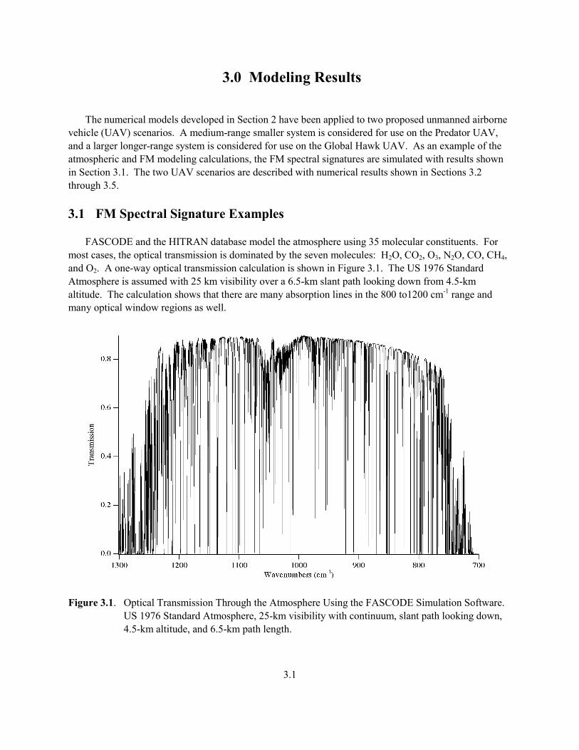
3.0 Modeling Results The numerical models developed in Section 2 have been applied to two proposed unmanned airborne vehicle (UAV) scenarios. A medium-range smaller system is considered for use on the Predator UAV, and a larger longer-range system is considered for use on the Global Hawk UAV. As an example of the atmospheric and FM modeling calculations, the FM spectral signatures are simulated with results shown in Section 3.1. The two UAV scenarios are described with numerical results shown in Sections 3.2 through 3.5. 3.1 FM Spectral Signature Examples FASCODE and the HITRAN database model the atmosphere using 35 molecular constituents. For most cases, the optical transmission is dominated by the seven molecules: H2O, CO2, O3, N2O, CO, CH4, and O2. A one-way optical transmission calculation is shown in Figure 3.1. The US 1976 Standard Atmosphere is assumed with 25 km visibility over a 6.5-km slant path looking down from 4.5-km altitude. The calculation shows that there are many absorption lines in the 800 to1200 cm-1 range and many optical window regions as well.

Figure 3.1. Optical Transmission Through the Atmosphere Using the FASCODE Simulation Software.

US 1976 Standard Atmosphere, 25-km visibility with continuum, slant path looking down, 4.5-km altitude, and 6.5-km path length.

3.2

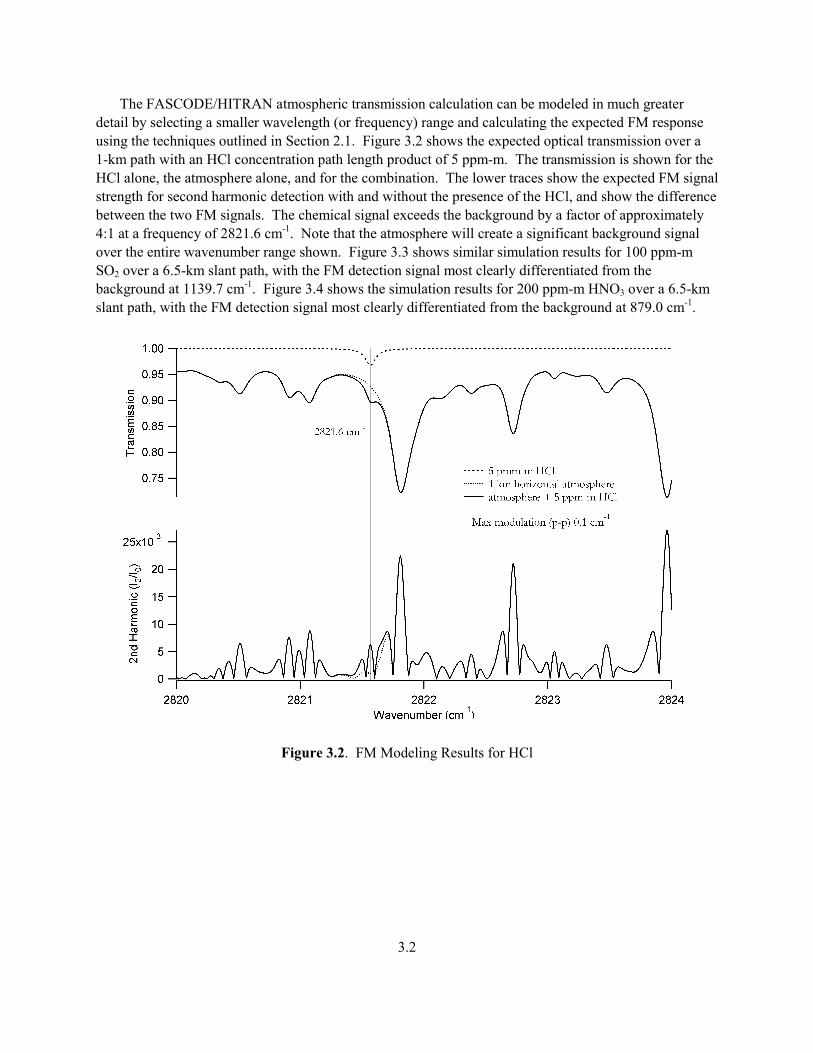
The FASCODE/HITRAN atmospheric transmission calculation can be modeled in much greater detail by selecting a smaller wavelength (or frequency) range and calculating the expected FM response using the techniques outlined in Section 2.1. Figure 3.2 shows the expected optical transmission over a 1-km path with an HCl concentration path length product of 5 ppm-m. The transmission is shown for the HCl alone, the atmosphere alone, and for the combination. The lower traces show the expected FM signal strength for second harmonic detection with and without the presence of the HCl, and show the difference between the two FM signals. The chemical signal exceeds the background by a factor of approximately 4:1 at a frequency of 2821.6 cm-1. Note that the atmosphere will create a significant background signal over the entire wavenumber range shown. Figure 3.3 shows similar simulation results for 100 ppm-m SO2 over a 6.5-km slant path, with the FM detection signal most clearly differentiated from the background at 1139.7 cm-1. Figure 3.4 shows the simulation results for 200 ppm-m HNO3 over a 6.5-km slant path, with the FM detection signal most clearly differentiated from the background at 879.0 cm-1.

Figure 3.2. FM Modeling Results for HCl

3.3

Figure 3.3. FM Modeling Results for SO2

Figure 3.4. FM Modeling Results for HNO3

3.4

3.2 UAV Scenarios Two UAV scenarios have been selected to represent possible deployment scenarios for a FM spectroscopy based sensor. The Predator scenario represents a medium range system using relatively compact optics (10 cm diameter receive telescope). The Global Hawk scenario represents a long range system using larger optics (20 cm diameter receive telescope). The operational and platform parameters for the two scenarios are detailed in Tables 3.1 and 3.2.

Table 3.1. Predator UAV Operational Parameters

Predator UAV Scenario Slant Range 6.5 km Altitude 4.5 km Speed 35 m/sec Optical Aperture 10 cm

Table 3.2. Global Hawk UAV Operational Parameters

Global Hawk UAV Scenario

Slant Range 30 km Altitude 20 km Speed 200 m/sec Optical Aperture 20 cm

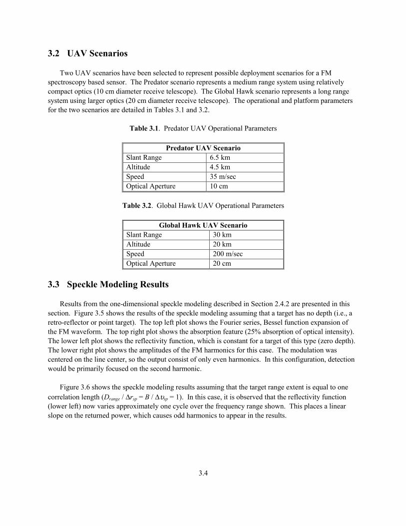
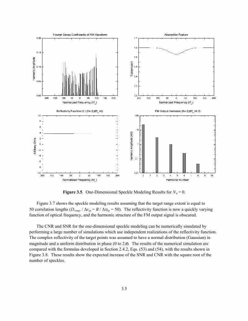
3.3 Speckle Modeling Results Results from the one-dimensional speckle modeling described in Section 2.4.2 are presented in this section. Figure 3.5 shows the results of the speckle modeling assuming that a target has no depth (i.e., a retro-reflector or point target). The top left plot shows the Fourier series, Bessel function expansion of the FM waveform. The top right plot shows the absorption feature (25% absorption of optical intensity). The lower left plot shows the reflectivity function, which is constant for a target of this type (zero depth). The lower right plot shows the amplitudes of the FM harmonics for this case. The modulation was centered on the line center, so the output consist of only even harmonics. In this configuration, detection would be primarily focused on the second harmonic. Figure 3.6 shows the speckle modeling results assuming that the target range extent is equal to one correlation length (Drange / ∆rsp = B / ∆υsp = 1). In this case, it is observed that the reflectivity function (lower left) now varies approximately one cycle over the frequency range shown. This places a linear slope on the returned power, which causes odd harmonics to appear in the results.

3.5

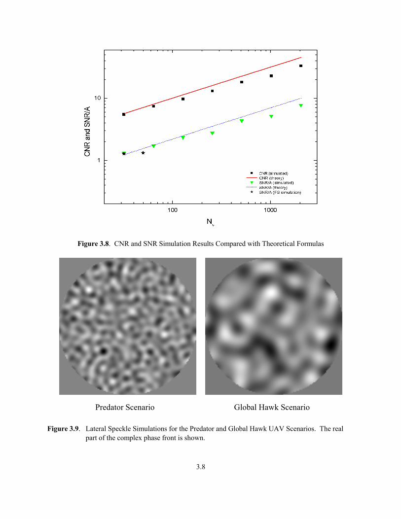
Figure 3.5. One-Dimensional Speckle Modeling Results for Nυ = 0. Figure 3.7 shows the speckle modeling results assuming that the target range extent is equal to 50 correlation lengths (Drange / ∆rsp = B / ∆υsp = 50). The reflectivity function is now a quickly varying function of optical frequency, and the harmonic structure of the FM output signal is obscured. The CNR and SNR for the one-dimensional speckle modeling can be numerically simulated by performing a large number of simulations which use independent realizations of the reflectivity function. The complex reflectivity of the target points was assumed to have a normal distribution (Gaussian) in magnitude and a uniform distribution in phase (0 to 2π). The results of the numerical simulation are compared with the formulas developed in Section 2.4.2, Eqs. (53) and (54), with the results shown in Figure 3.8. These results show the expected increase of the SNR and CNR with the square root of the number of speckles.

3.6

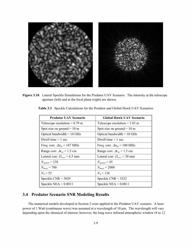
Figure 3.6. One-Dimensional Speckle Modeling Results for Nυ = 1 Three-dimensional speckled wavefront simulations are shown in Figures 3.9 and 3.10. In Figure 3.9, the real part of the complex wavefront is shown for both the Predator and Global Hawk UAV scenarios. The speckle correlation parameters and results are shown in Table 3.3 for both scenarios. The expected result of more spatial speckle in the Predator scenario than in the Global Hawk scenario is observed in the figure (Nspatial = 238 vs. Nspatial = 45). The intensity at the telescope aperture and at the focal plane for the Predator scenario is shown in Figure 3.10. The modeling program generates a video animation of the results, with each frame representing a particular optical frequency. By playing the animation, the qualitative behavior of the speckle with frequency is observed. The intensity at the telescope aperture animation was particularly interesting. The speckle pattern was observed to scroll vertically as the frequency was varied. As the speckle pattern shifted, it would also vary slightly in shape and pattern. The target reflectivity distribution

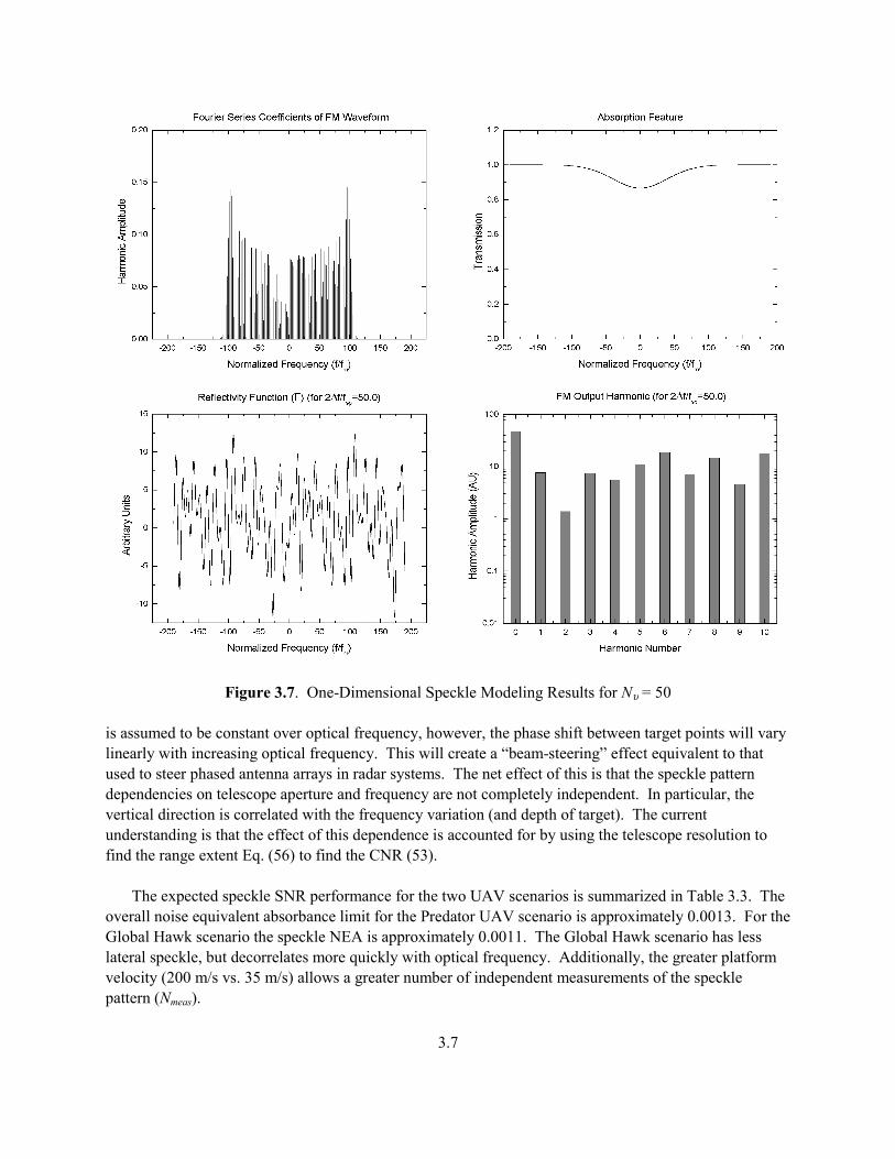
3.7

Figure 3.7. One-Dimensional Speckle Modeling Results for Nυ = 50 is assumed to be constant over optical frequency, however, the phase shift between target points will vary linearly with increasing optical frequency. This will create a “beam-steering” effect equivalent to that used to steer phased antenna arrays in radar systems. The net effect of this is that the speckle pattern dependencies on telescope aperture and frequency are not completely independent. In particular, the vertical direction is correlated with the frequency variation (and depth of target). The current understanding is that the effect of this dependence is accounted for by using the telescope resolution to find the range extent Eq. (56) to find the CNR (53). The expected speckle SNR performance for the two UAV scenarios is summarized in Table 3.3. The overall noise equivalent absorbance limit for the Predator UAV scenario is approximately 0.0013. For the Global Hawk scenario the speckle NEA is approximately 0.0011. The Global Hawk scenario has less lateral speckle, but decorrelates more quickly with optical frequency. Additionally, the greater platform velocity (200 m/s vs. 35 m/s) allows a greater number of independent measurements of the speckle pattern (Nmeas).

3.8

Figure 3.8. CNR and SNR Simulation Results Compared with Theoretical Formulas

Predator Scenario Global Hawk Scenario Figure 3.9. Lateral Speckle Simulations for the Predator and Global Hawk UAV Scenarios. The real

part of the complex phase front is shown.

3.9

Figure 3.10. Lateral Speckle Simulations for the Predator UAV Scenario. The intensity at the telescope

aperture (left) and at the focal plane (right) are shown.

Table 3.3. Speckle Calculations for the Predator and Global Hawk UAV Scenarios

Predator UAV Scenario Global Hawk UAV Scenario Telescope resolution = 0.79 m Telescope resolution = 1.83 m Spot size on ground = 10 m Spot size on ground = 10 m Optical bandwidth = 10 GHz Optical bandwidth = 10 GHz Dwell time = 1 sec. Dwell time = 1 sec.

Freq. corr. ∆υsp = 187 MHz Freq. corr. ∆υsp = 100 MHz

Range corr. ∆rsp = 1.5 cm Range corr. ∆rsp = 1.5 cm Lateral corr. Dcorr = 6.5 mm Lateral corr. Dcorr = 30 mm Nspatial = 238 Nspatial = 45 Nmeas = 700 Nmeas = 2000

Nυ = 55 Nυ = 136 Speckle CNR = 3029 Speckle CNR = 3522 Speckle NEA = 0.0013 Speckle NEA = 0.0011

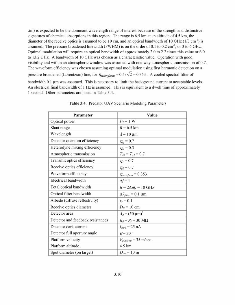
3.4 Predator Scenario SNR Modeling Results The numerical models developed in Section 2 were applied to the Predator UAV scenario. A laser power of 1 Watt (continuous wave) was assumed at a wavelength of 10 µm. The wavelength will vary depending upon the chemical of interest; however, the long wave infrared atmospheric window (8 to 12

3.10

µm) is expected to be the dominant wavelength range of interest because of the strength and distinctive signatures of chemical absorptions in this region. The range is 6.5 km at an altitude of 4.5 km, the diameter of the receive optics is assumed to be 10 cm, and an optical bandwidth of 10 GHz (1/3 cm-1) is assumed. The pressure broadened linewidth (FWHM) is on the order of 0.1 to 0.2 cm-1, or 3 to 6 GHz. Optimal modulation will require an optical bandwidth of approximately 2.0 to 2.2 times this value or 6.0 to 13.2 GHz. A bandwidth of 10 GHz was chosen as a characteristic value. Operation with good visibility and within an atmospheric window was assumed with one-way atmospheric transmission of 0.7. The waveform efficiency was chosen assuming optimal modulation using first harmonic detection on a pressure broadened (Lorentzian) line, for 353.02/5.0 ==waveformη . A cooled spectral filter of

bandwidth 0.1 µm was assumed. This is necessary to limit the background current to acceptable levels. An electrical final bandwidth of 1 Hz is assumed. This is equivalent to a dwell time of approximately 1 second. Other parameters are listed in Table 3.4.

Table 3.4. Predator UAV Scenario Modeling Parameters

Parameter Value Optical power PT = 1 W Slant range R = 6.5 km Wavelength λ = 10 µm Detector quantum efficiency ηQ = 0.7 Heterodyne mixing efficiency ηH = 0.3 Atmospheric transmission TA1 = TA2 = 0.7 Transmit optics efficiency ηT = 0.7 Receive optics efficiency ηR = 0.7 Waveform efficiency ηwaveform = 0.353 Electrical bandwidth ∆f = 1 Total optical bandwidth B = 2∆ωm = 10 GHz Optical filter bandwidth ∆λfilter = 0.1 µm Albedo (diffuse reflectivity) εr = 0.1 Receive optics diameter DC = 10 cm Detector area Ad = (50 µm)2 Detector and feedback resistances Rd = Rf = 30 MΩ Detector dark current Idark = 25 nA Detector full aperture angle θ = 30° Platform velocity Vplatform = 35 m/sec Platform altitude 4.5 km Spot diameter (on target) Dtar = 10 m

3.11

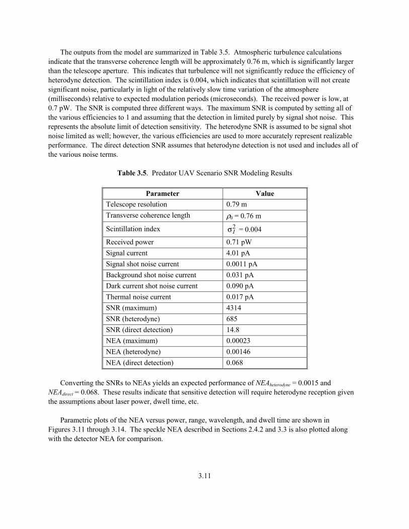
The outputs from the model are summarized in Table 3.5. Atmospheric turbulence calculations indicate that the transverse coherence length will be approximately 0.76 m, which is significantly larger than the telescope aperture. This indicates that turbulence will not significantly reduce the efficiency of heterodyne detection. The scintillation index is 0.004, which indicates that scintillation will not create significant noise, particularly in light of the relatively slow time variation of the atmosphere (milliseconds) relative to expected modulation periods (microseconds). The received power is low, at 0.7 pW. The SNR is computed three different ways. The maximum SNR is computed by setting all of the various efficiencies to 1 and assuming that the detection in limited purely by signal shot noise. This represents the absolute limit of detection sensitivity. The heterodyne SNR is assumed to be signal shot noise limited as well; however, the various efficiencies are used to more accurately represent realizable performance. The direct detection SNR assumes that heterodyne detection is not used and includes all of the various noise terms.

Table 3.5. Predator UAV Scenario SNR Modeling Results

Parameter Value Telescope resolution 0.79 m Transverse coherence length ρ0 = 0.76 m

Scintillation index 2Iσ = 0.004

Received power 0.71 pW Signal current 4.01 pA Signal shot noise current 0.0011 pA Background shot noise current 0.031 pA Dark current shot noise current 0.090 pA Thermal noise current 0.017 pA SNR (maximum) 4314 SNR (heterodyne) 685 SNR (direct detection) 14.8 NEA (maximum) 0.00023 NEA (heterodyne) 0.00146 NEA (direct detection) 0.068

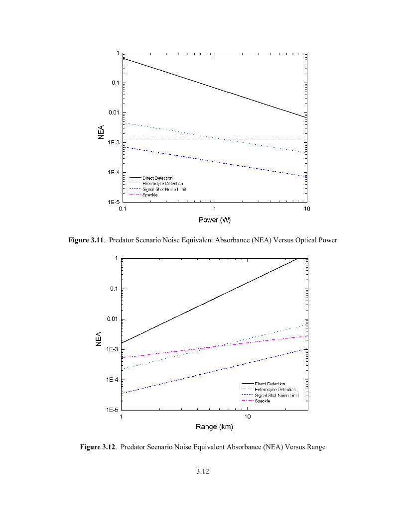
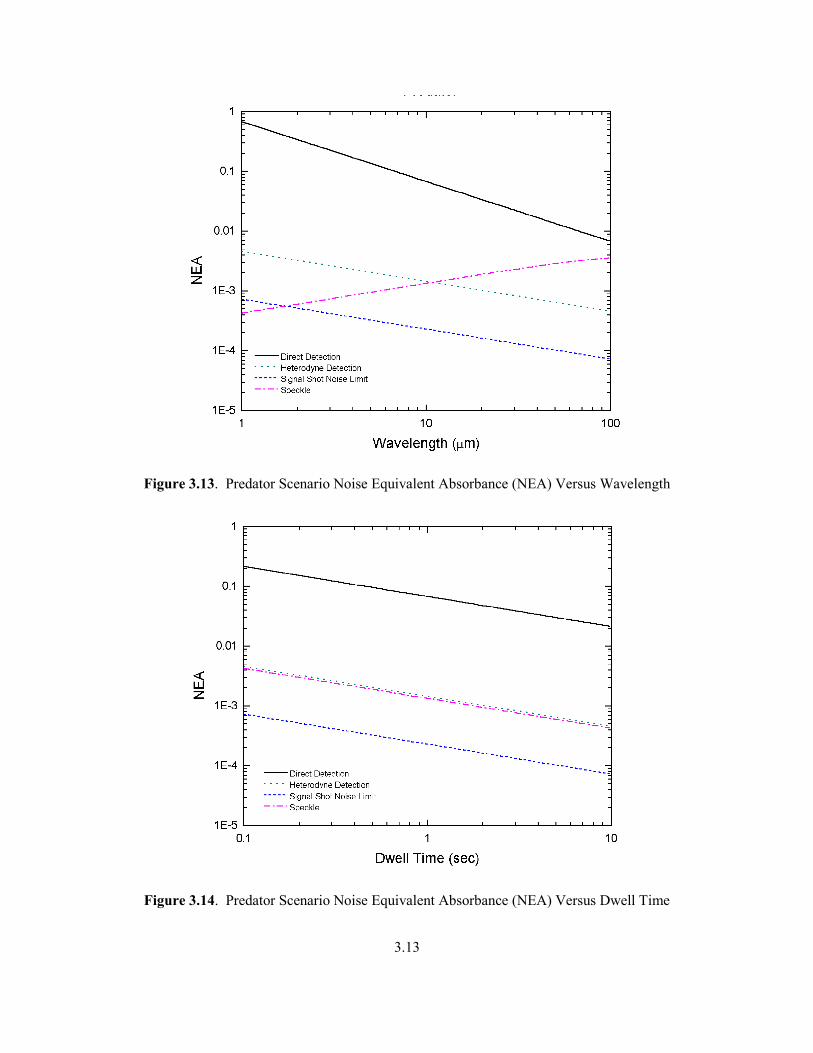
Converting the SNRs to NEAs yields an expected performance of NEAheterodyne = 0.0015 and NEAdirect = 0.068. These results indicate that sensitive detection will require heterodyne reception given the assumptions about laser power, dwell time, etc. Parametric plots of the NEA versus power, range, wavelength, and dwell time are shown in Figures 3.11 through 3.14. The speckle NEA described in Sections 2.4.2 and 3.3 is also plotted along with the detector NEA for comparison.

3.12

Figure 3.11. Predator Scenario Noise Equivalent Absorbance (NEA) Versus Optical Power

Figure 3.12. Predator Scenario Noise Equivalent Absorbance (NEA) Versus Range

3.13

Figure 3.13. Predator Scenario Noise Equivalent Absorbance (NEA) Versus Wavelength

Figure 3.14. Predator Scenario Noise Equivalent Absorbance (NEA) Versus Dwell Time

3.14

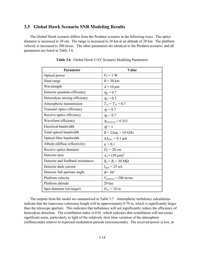
3.5 Global Hawk Scenario SNR Modeling Results The Global Hawk scenario differs from the Predator scenario in the following ways. The optics diameter is increased to 20 cm. The range is increased to 30 km at an altitude of 20 km. The platform velocity is increased to 200 m/sec. The other parameters are identical to the Predator scenario, and all parameters are listed in Table 3.6.

Table 3.6. Global Hawk UAV Scenario Modeling Parameters

Parameter Value Optical power PT = 1 W Slant range R = 30 km Wavelength λ = 10 µm Detector quantum efficiency ηQ = 0.7 Heterodyne mixing efficiency ηH = 0.3 Atmospheric transmission TA1 = TA2 = 0.7 Transmit optics efficiency ηT = 0.7 Receive optics efficiency ηR = 0.7 Waveform efficiency ηwaveform = 0.353 Electrical bandwidth ∆f = 1 Total optical bandwidth B = 2∆ωm = 10 GHz Optical filter bandwidth ∆λfilter = 0.1 µm Albedo (diffuse reflectivity) εr = 0.1 Receive optics diameter DC = 20 cm Detector area Ad = (50 µm)2 Detector and feedback resistances Rd = Rf = 30 MΩ Detector dark current Idark = 25 nA Detector full aperture angle θ = 30° Platform velocity Vplatform = 200 m/sec Platform altitude 20 km Spot diameter (on target) Dtar = 10 m

The outputs from the model are summarized in Table 3.7. Atmospheric turbulence calculations indicate that the transverse coherence length will be approximately 0.70 m, which is significantly larger than the telescope aperture. This indicates that turbulence will not significantly reduce the efficiency of heterodyne detection. The scintillation index is 0.01, which indicates that scintillation will not create significant noise, particularly in light of the relatively slow time variation of the atmosphere (milliseconds) relative to expected modulation periods (microseconds). The received power is low, at

3.15

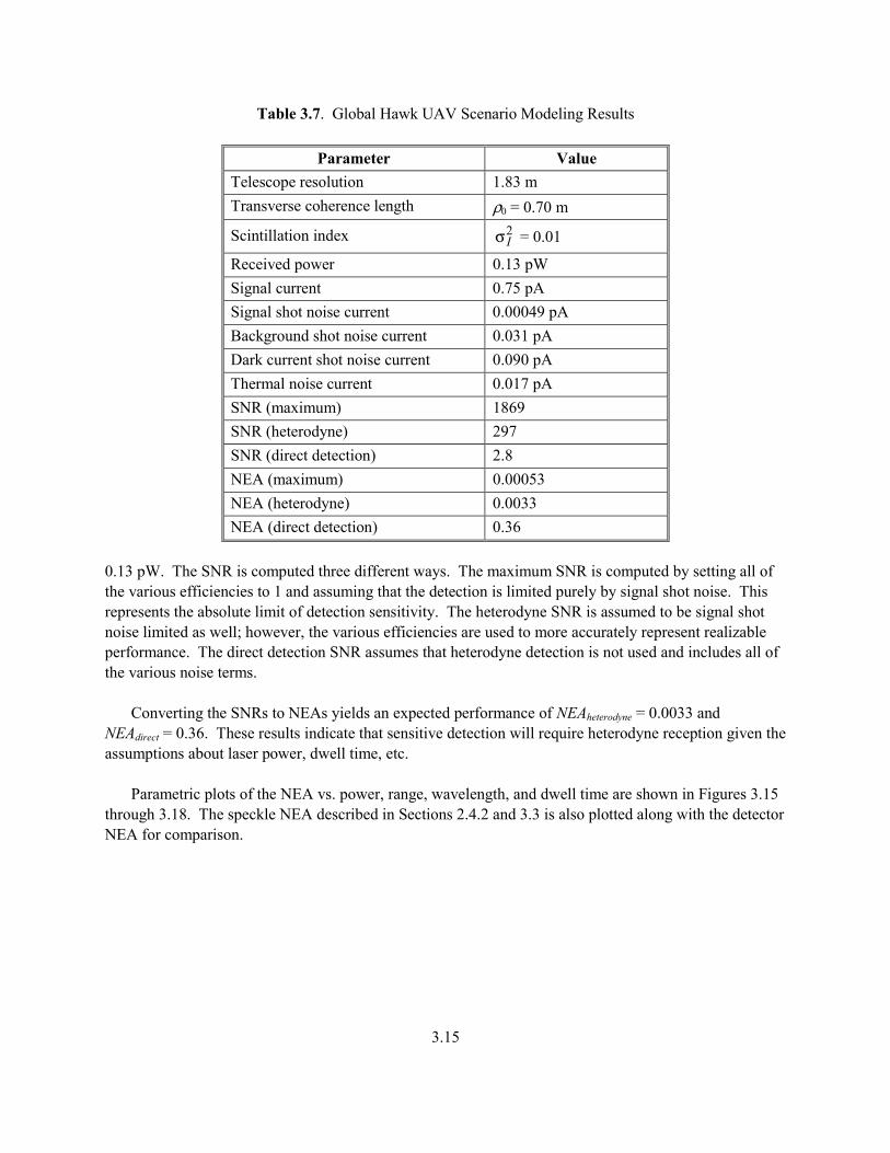
Table 3.7. Global Hawk UAV Scenario Modeling Results

Parameter Value Telescope resolution 1.83 m Transverse coherence length ρ0 = 0.70 m

Scintillation index 2Iσ = 0.01

Received power 0.13 pW Signal current 0.75 pA Signal shot noise current 0.00049 pA Background shot noise current 0.031 pA Dark current shot noise current 0.090 pA Thermal noise current 0.017 pA SNR (maximum) 1869 SNR (heterodyne) 297 SNR (direct detection) 2.8 NEA (maximum) 0.00053 NEA (heterodyne) 0.0033 NEA (direct detection) 0.36

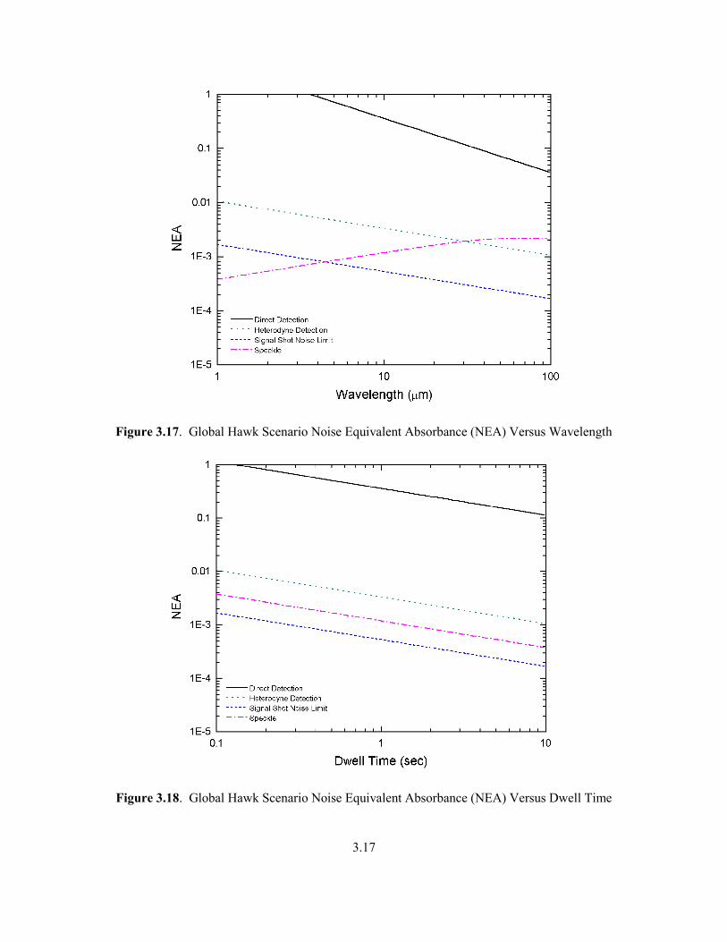
0.13 pW. The SNR is computed three different ways. The maximum SNR is computed by setting all of the various efficiencies to 1 and assuming that the detection is limited purely by signal shot noise. This represents the absolute limit of detection sensitivity. The heterodyne SNR is assumed to be signal shot noise limited as well; however, the various efficiencies are used to more accurately represent realizable performance. The direct detection SNR assumes that heterodyne detection is not used and includes all of the various noise terms. Converting the SNRs to NEAs yields an expected performance of NEAheterodyne = 0.0033 and NEAdirect = 0.36. These results indicate that sensitive detection will require heterodyne reception given the assumptions about laser power, dwell time, etc. Parametric plots of the NEA vs. power, range, wavelength, and dwell time are shown in Figures 3.15 through 3.18. The speckle NEA described in Sections 2.4.2 and 3.3 is also plotted along with the detector NEA for comparison.

3.16

Figure 3.15. Global Hawk Scenario Noise Equivalent Absorbance (NEA) Versus Optical Power

Figure 3.16. Global Hawk Scenario Noise Equivalent Absorbance (NEA) Versus Range

3.17

Figure 3.17. Global Hawk Scenario Noise Equivalent Absorbance (NEA) Versus Wavelength

Figure 3.18. Global Hawk Scenario Noise Equivalent Absorbance (NEA) Versus Dwell Time

4.1

4.0 Modeling and Validation Issues and Conclusions The FM modeling work discussed in Sections 2 and 3 has raised several issues that need to be addressed with future modeling and experimental work. These include system sensitivity, target-induced speckle, heterodyne detection, and determination of the system architecture. 4.1 Sensitivity High-power lasers coupled with highly sensitive detection will be required to perform remote chemical detection based on FM spectroscopy. The results presented in Section 3 assumed that diffuse scattering hard targets were used, as would be expected in uncontrolled environments. Estimates for returned signal power are in the range of 0.1 to 1.0 pW. FM spectroscopy requires that the noise level be several orders of magnitude below this level for sensitive detection. The numerical results indicate that this will only be possible using coherent (heterodyne) detection. The numerical results indicate that by using heterodyne detection, it may be possible to detect chemicals that have absorbances several times larger than the noise equivalent absorbance, which is on the order of 10-3. The detection limit is primarily caused by the very low level of optical power returned to the system. Operating scenarios that make use of retro-reflectors or bi-static operation will increase the expected optical power by several orders of magnitude, most likely eliminating the need for heterodyne detection. 4.2 Target-Induced Speckle The speckle analysis presented in Sections 2 and 3 indicates that speckle may limit the ultimate noise equivalent absorbance to levels on the order of 10-3. This performance can be increased by using a larger illuminated spot on the ground and by using larger telescope apertures. The formulas presented in Section 2.4.2 agree with those developed for conventional DIAL (MacKerrow et al. 1996; Schmitt and McVey 1996) with the addition of a third term that accounts for the decorrelation of the speckle as the frequency is modulated. Speckle also has a detrimental effect on the performance of a heterodyne system. Efficient heterodyne detection requires that the signal beam’s wavefront be phase-aligned with the local oscillator (LO) beam’s wavefront. A speckled wavefront varies in phase from 0 to 2π over a spatial scale of the speckle correlation diameter Dcorr, as shown in Figures 3.9 and 3.10. The resulting heterodyne signal will be diminished because of destructive coherent interference from the numerous speckle lobes. Kamerman indicates that this effect can be accounted for by replacing the receive telescope aperture with an effective aperture which is the geometric mean of the telescope aperture Drec and the speckle correlation diameter Dcorr, Corrreceff DDD = (Kamerman 1993). If the system has been designed to reduce the speckle noise by using a large illuminated spot coupled with a large telescope aperture, this will cause a significant reduction in received signal strength. The speckle noise may not be averaged down as expected because the speckle analysis assumed incoherent averaging of the energy within each speckle lobe, as would occur with conventional direct detection.

4.2

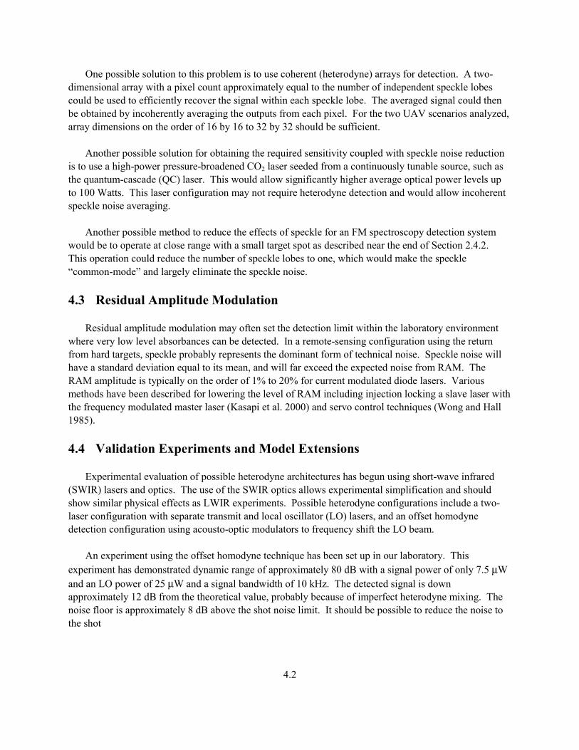
One possible solution to this problem is to use coherent (heterodyne) arrays for detection. A two-dimensional array with a pixel count approximately equal to the number of independent speckle lobes could be used to efficiently recover the signal within each speckle lobe. The averaged signal could then be obtained by incoherently averaging the outputs from each pixel. For the two UAV scenarios analyzed, array dimensions on the order of 16 by 16 to 32 by 32 should be sufficient. Another possible solution for obtaining the required sensitivity coupled with speckle noise reduction is to use a high-power pressure-broadened CO2 laser seeded from a continuously tunable source, such as the quantum-cascade (QC) laser. This would allow significantly higher average optical power levels up to 100 Watts. This laser configuration may not require heterodyne detection and would allow incoherent speckle noise averaging. Another possible method to reduce the effects of speckle for an FM spectroscopy detection system would be to operate at close range with a small target spot as described near the end of Section 2.4.2. This operation could reduce the number of speckle lobes to one, which would make the speckle “common-mode” and largely eliminate the speckle noise. 4.3 Residual Amplitude Modulation Residual amplitude modulation may often set the detection limit within the laboratory environment where very low level absorbances can be detected. In a remote-sensing configuration using the return from hard targets, speckle probably represents the dominant form of technical noise. Speckle noise will have a standard deviation equal to its mean, and will far exceed the expected noise from RAM. The RAM amplitude is typically on the order of 1% to 20% for current modulated diode lasers. Various methods have been described for lowering the level of RAM including injection locking a slave laser with the frequency modulated master laser (Kasapi et al. 2000) and servo control techniques (Wong and Hall 1985). 4.4 Validation Experiments and Model Extensions Experimental evaluation of possible heterodyne architectures has begun using short-wave infrared (SWIR) lasers and optics. The use of the SWIR optics allows experimental simplification and should show similar physical effects as LWIR experiments. Possible heterodyne configurations include a two-laser configuration with separate transmit and local oscillator (LO) lasers, and an offset homodyne detection configuration using acousto-optic modulators to frequency shift the LO beam. An experiment using the offset homodyne technique has been set up in our laboratory. This experiment has demonstrated dynamic range of approximately 80 dB with a signal power of only 7.5 µW and an LO power of 25 µW and a signal bandwidth of 10 kHz. The detected signal is down approximately 12 dB from the theoretical value, probably because of imperfect heterodyne mixing. The noise floor is approximately 8 dB above the shot noise limit. It should be possible to reduce the noise to the shot

4.3

noise limit by increasing the LO power. It may be more difficult to improve the heterodyne mixing efficiency, but gains of several dB are likely. This sensitive detection should allow sub-picowatt sensitivity. Additional experiments are planned to evaluate the accuracy of the speckle and detector SNR formulations given in Section 2. To validate the speckle SNR formulas, it will probably be necessary to build a moderate range (up to 1 to 2 km) FM LIDAR system. The frequency-dependent speckle phenomenon is not easily observed in the laboratory because the range extent within the lateral resolution is small. This is the result of the relatively high lateral resolution of the system at closer ranges. The modeling can be improved by careful comparison of theoretical predictions with measured performance. Some of the required experiments can be performed in the laboratory, while others may require the development of a moderate range system (up to 1 to 2 km). The moderate range system could be a portable laboratory experiment operated outdoors or a trailer-based system.

5.1

5.0 Acknowledgments The work described in this report was supported by funding from several sources. The mathematical development of the model was supported with internal funding through the Infrared Chemical Sensor Laboratory Directed Research and Development (LDRD) project. The application of the model to the two UAV scenarios and subsequent numerical results were supported by Defense Advanced Research Projects Agency (DARPA) Concepts for the Tactical Multi-Mode Laser (MML) project, and by the U.S. Department of Energy (DOE) NN-20 Office, through the Hybrid Prototype Airborne Infrared (HYPAIR) project.

6.1

6.0 References Abarbanel, H., S. Drell, N. Fortson, J. Goodman, S. Koonin, N. Lewis, G. MacDonald, C. Max, S. Ride, J. Sullivan, and F. Zachariasen. 1994. Lidar, JASON - The Mitre Corporation. Andrews, L. C., and R. L. Phillips. 1998. Laser Beam Propagation through Random Media. SPIE Optical Engineering Press, 2. Beland, R. R. 1993. Propagation through Atmospheric Optical Turbulence, Ch. 2. Atmospheric Propagation of Atmospheric Radiation. J. S. Acetta, D. L. Shumaker, and F. G. Smith, SPIE Optical Engineering Press, Bellingham, Washington. Capasso, F., C. Gmachl, et al. 1999. “Quantum Cascade Lasers.” Physics World 12(6):27-33. Carlisle, C. B., D. E. Cooper, et al. 1989. “Quantum Noise-Limited FM Spectroscopy with a Lead-Salt Diode Laser.” Applied Optics 28(13):2567-2576. Fante, R. L. 1975. “Electromagnetic Beam Propagation in Turbulent Media.” Proceedings of the IEEE 63(12):1669-1692. Gehrtz, M., G. C. Bjorklund, et al. 1985. “Quantum-Limited Laser Frequency-Modulation Spectroscopy.” Journal of the Optical Society of America B (Optical Physics) 2(9):1510-26. Gehrtz, M., W. Lenth, et al. 1986. “High-Frequency-Modulation Spectroscopy with a Lead-Salt Diode Laser.” Optics Letters 11(3):132-4. Gmachl, C., F. Capasso, et al. 2000. “High-Power, Continuous-Wave, Current-Tunable, Single-mode quantum-cascade distributed-feedback lasers at Lambda Equivalent to 5.2 and Lambda Equivalent to 7.95 µm.” Optics Letters 25(4):230-2. Kamerman, G. W. 1993. Laser Radar, Ch. 1. Active Electro-Optical Systems. J. S. Acetta, D. L. Shumaker, and C. S. Fox, SPIE Optical Engineering Press, 6. Kasapi, S., S. Lathi, et al. 2000. “Sub-Shot-Noise Frequency-Modulation Spectroscopy by Use of Amplitude-Squeezed Light from Semiconductor Lasers.” Journal of the Optical Society of America B (Optical Physics) 17(2):275-9. Lenth, W. 1984. “High Frequency Heterodyne Spectroscopy with Current-Modulated Diode Lasers.” IEEE Journal of Quantum Electronics QE-20(9):1045-50. MacKerrow, E. P., G. Busch, J. J. Tiee, M. J. Schmitt, et. al. 1995. “Field Measurements of Laser Speckle Effects on CO2 DIAL.” CALIOPE ITR Proceedings, p. 147-155.

6.2

MacKerrow, E. P., J. J. Tiee, M. J. Schmitt, M. C. Whihtehead, C. R. Quick, and C. B. Fite. 1996. “Measurements of Temporal Autocorrelation Effects on CO2 DIAL Signal Averaging Statistics.” CALIOPE ITR Proceedings, p. 371-393. Miller, J. L., and E. Friedman. 1996. Photonics Rules of Thumb, McGraw-Hill. Petrin, R. R., et. al. 1996. “Effects on DIAL Sensitivity: Atmospheric Phenomena.” CALIOPE ITR Proceeding, p 149-163. Schmitt, M., and B. McVey. 1996. “Enhancements to the SONDIAL Lidar Design Code.” CALIOPE ITR Proceedings, p. 361-370. Silver, J. A. 1992. “Frequency-Modulation Spectroscopy for Trace Species Detection: Theory and Comparison Among Experimental Methods.” Applied Optics 31(6):707-17. Silver, J. A., and A. C. Stanton. 1988. “Two-Tone Optical Heterodyne Spectroscopy Using Buried Double Heterostructure Lead-Salt Diode Lasers.” Applied Optics 27(21):4438-44. Tyson, R. K. 1998. Principles of Adaptive Optics, Academic Press. Tyson, R. K., and P. B. Ulrich. 1993. Adaptive Optics, Ch. 2. Emerging Systems and Technologies. J. S. Acetta, D. L. Shumaker, and S. R. Robinson, SPIE Optical Engineering Press, 8. Wong, N. C., and J. L. Hall. 1985. “Servo Control of Amplitude Modulation in Frequency-Modulation Spectroscopy: Demonstration of Shot-Noise-Limited Detection.” Journal of the Optical Society of America B (Optical Physics) 2(9):1527-33. Yariv, A. 1991. Optical Electronics, Saunders College Publishing.