Frequency fluctuationsin power systems

Student:Szabolcs Horvát

Advisor:László P. Csernai

University of BergenJune, 2007

Abstract

A basic difficulty with using and producing electric energy is that—apart from short periods of time and small quantities—electric en-ergy cannot be stored. It must be produced at the same time as itis used. To maintain the balance between power production andconsumption, the power plants that produce the energy must becontinuously regulated.

Power system control is based on the phenomenon that in case ofan imbalance, the AC frequency of the network changes. Duringnormal operation of the electric grid, the system frequency keptnear a set value, but it is allowed to fluctuate within certain bound.

In this work we survey the causes of frequency fluctuations, andexplore the possibility of gathering information about the state of thesystem (and perhaps increasing control performance) by measuringthese fluctuations.

We reach the conclusion that frequency fluctuations are mainlycaused by random demand changes in the system, but their natureis also influenced by the state of the generators that are participatingin power control.

1

Acknowledgements

I am indebted to my supervisor, Professor László P. Csernai, for hisprofessional guidance, but also for his encouragement and supportthroughout the past year. Without his help I would not have beenable to complete this work.

I would like to thank Hermod Nitter, my companion in this project,for useful discussions on the topic of power system control.

The Quota Scholarship provided by the Norwegian Governmentmade it possible for me to study at the University of Bergen.

But my greatest gratitude goes to my mother and father for their un-derstanding, and the emotional support they provided, even while Iwas far from home.

June, 2007

Szabolcs Horvát

2

Contents

1 Notations and basics 41.1 Alternating current (AC) . . . . . . . . . . . . . . . . . . . . . . . . . 4

1.1.1 Reactance . . . . . . . . . . . . . . . . . . . . . . . . . . . . . 51.1.2 The phasor representation . . . . . . . . . . . . . . . . . . . 51.1.3 Impedance . . . . . . . . . . . . . . . . . . . . . . . . . . . . . 61.1.4 AC power . . . . . . . . . . . . . . . . . . . . . . . . . . . . . . 7

1.2 Generators . . . . . . . . . . . . . . . . . . . . . . . . . . . . . . . . . 81.2.1 A simple generator . . . . . . . . . . . . . . . . . . . . . . . . 81.2.2 The synchronous machine . . . . . . . . . . . . . . . . . . . 91.2.3 Coupling of generators . . . . . . . . . . . . . . . . . . . . . . 12

2 Power system control 132.1 Practical governor models . . . . . . . . . . . . . . . . . . . . . . . . 16

2.1.1 The flyball governor . . . . . . . . . . . . . . . . . . . . . . . 162.1.2 Speed droop governor . . . . . . . . . . . . . . . . . . . . . . 19

3 Data analysis and simulations 213.1 Data sources . . . . . . . . . . . . . . . . . . . . . . . . . . . . . . . . 213.2 Description of the model . . . . . . . . . . . . . . . . . . . . . . . . 223.3 Simulation results . . . . . . . . . . . . . . . . . . . . . . . . . . . . . 29

4 Summary 37

Bibliography 38

3

θB

A

Figure 1: Rotating wire loop in magnetic field.

1 Notations and basics

1.1 Alternating current (AC)

The simplest possible electric generator is a rectangular wire loop that is rotatingin a homogeneous magnetic field. Since the sides of the loop are moving, thefree charges inside experience a Lorentz force, and an electric current is induced.

Let us calculate the induced electromotive force! To make the calculationssimpler, we shall analyse this system from the rotating reference frame attachedto the wire loop.

According to Faraday’s law of induction, the integral of the electric field Earound a loop C is proportional to the rate of change of magnetic flux throughthe surface S enclosed by the loop:∮

CE ·d l =− d

d t

∫S

B ·dS.

If the area enclosed by the loop is A, and the angle between the surface normalof the wire loop and the magnetic field is denoted by ϑ, the electromotive forceinduced in the loop will be V = ∫

C E ·d l = − dd t AB cosϑ = AB ϑsinϑ. The dot

indicates the time derivative. If the loop is rotating with a steady angular velocity

4

ω, the induced voltage will vary harmonically:

V = ABωsinωt .

1.1.1 Reactance

Let us look at the relation between voltage and current in the case of simplecircuit elements!

The voltage measured between the poles of a resistor is related to the currentby Ohm’s law: V = R · I .

The voltage on a capacitor is proportional to the charge Q carried by it,V =Q/C , hence the current is proportional to the time derivative of the voltage:I = Q = CV . In the case of sinusoidally alternating voltage, the current variessinusoidally too, but it lags behind by a quarter cycle:

I =Cd

d tV0 cosωt =−CωV0 sinωt = V0

XCsinωt .

The quantity XC =−1/ωC is called capacitive reactance.When the current in an inductor (coil) changes, an electromotive force that

is proportional to the rate of this change is induced. The voltage measuredbetween the poles of the inductor is V = LI . For a harmonically varying currentI = I0 sinωt , the voltage is

V = Ld

d tI0 sinωt = LωI0 cosωt = I0XL cosωt ,

so the phase difference between V and I is the opposite as in the case of acapacitor. The quantity XL =ωL is called inductive reactance.

Reactance is similar to resistance in that it is the ratio of the peak values ofalternating voltage and current (it is measured in ohms), but it is used whenthere is a phase difference of ±π/2 between the two. Conventionally X is positivewhen the current is lagging behind the voltage.

1.1.2 The phasor representation

It is advantageous to treat harmonically varying quantities as the projection of arotating two dimensional vector. This way the peak amplitude is equal to thelength of the vector, while the phase difference between two quantities may bevisualised as the angle between two vectors (fig. 2).

When this vector is represented as a complex number, it is referred to as aphasor. To distinguish a complex phasor from the instantaneous value of the realquantity it represents, we shall write a tilde above it: V =V0e iϕ. The projectionis usually taken as the real part of phasors: V =ℜ(V ) =V0 cosωt .

5

V

I

C

I

L

I

R

R

C

L

Figure 2: The relative phases of currents passing through a resistor, an inductorand a capacitor connected in parallel.

Since projection is a linear operation, phasors may be added or multipliedby scalars just like any real-valued quantity, but care should be taken whenmultiplying them because ℜ(AB) 6= AB .

1.1.3 Impedance

An advantage of the phasor notation is that the relation between alternatingvoltage and current may be expressed in a form analogous to Ohm’s law. In thecase of a capacitor IC = C d

d t

(V0C e iωt

) = iωCV0C e iωt , so VC /IC = i XC . For aninductor, VL/IL = i XL .

The ratio of complex voltage and current is called impedance and is usuallydenoted by Z = V /I . It can be easily proven that the resulting impedance of morecomplicated circuits (e.g. series or parallel connection) can be calculated inexactly the same way as resistances. The real part of impedance is the resistance,while the imaginary part is the reactance: Z = R + i X .

The phase difference between the voltage measured on an element of impedanceZ and the current is ϕ = arg Z = arctan(X /R). The ratio of the peak values is

V0/I0 =√

(V V ∗)/(I I∗) = Z Z∗ = |Z | =p

R2 +X 2. (Z∗ denotes the complex con-jugate of Z .)

It should be noted that this simple mathematical notation is only usable forsystems in a steady state (i.e. for purely harmonically varying quantities). Eventhough the angular frequency, ω, is not explicitly written out in this description,the impedance of a non purely resistive element does depend on ω.

6

1.1.4 AC power

The power consumed by a circuit element is at any instant equal to the productof voltage and current: p =V · I .

In the resistive case P = I 2R = I 20 R sin2ωt = 1

2 I 20 R(1−cos2ωt). In practical

applications one usually deals with time scales much longer than 1/ω so let uscalculate the time average of dissipated power:

Pavg = 1

T2 −T1

∫ T2

T1

RI 2 d t = RI 2rms,

where T2 −T1 À 1/ω and

Irms =√

1

T2 −T1

∫ T2

T1

I 2 d t

is called the root mean square (RMS) value of the current. The RMS value of asinusoidally varying current is Irms = I0/

p2, and Pavg = 1

2 I 20 R. For AC voltage

and current, usually the RMS values are specified instead of the peak values V0

and I0.In the purely inductive or capacitive case P = V · I = I 2

0 X sinωt · cosωt =12 I 2

0 X sin2ωt . Note the instantaneous value of the power is oscillating betweenpositive and negative values, but the average is Pavg = 0. This means that thecircuit element in question consumes and releases energy periodically, but nopower is dissipated. Energy is temporarily stored as the energy of an inductor’smagnetic field or capacitor’s electric field.

In the general case of Z = R + i X , the phase difference between voltage andcurrent is ϕ= arctan(X /R) and

P =V · I =V0I0 sin(ωt +ϕ) · sinωt

= V0I0

2(1−cos2ωt ) ·cosϕ︸ ︷︷ ︸

p

+ V0I0

2sin2ωt · sinϕ︸ ︷︷ ︸

q

.

Both the amplitude and mean value of the first term, p, is P0 = VrmsIrms cosϕ,while the second term, q , has amplitude Q0 = VrmsIrms sinϕ but mean 0. pbehaves like the power dissipated in a pure resistor. It represents a non-zero netenergy flow, so it is called real power or active power. q is similar to the poweron a reactance: it represents an oscillating energy flow with mean 0. It is calledreactive power.

It is easy to check that the complex quantity S = Vrms · I∗rms is S = P0 + iQ0

(fig. 3). S is called the apparent power. Thus P0 = |S|cosϕ, where we call cosϕthe power factor.Power factors are usually described as “lagging” (when the

7

Reactive power, Q

₀

Real power, P₀

Apparent power, S

φ

Figure 3: The power triangle

current lags behind the voltage) or “leading” (in the opposite case) to indicatethe sign of ϕ.

Conventionally, a circuit element with Q0 > 0 is said to consume reactivepower while one with Q0 < is said to produce it. But it is important to note thatno net power is produced or consumed in this case. There is an asymmetry inthe interpretation of the magnitude of real and reactive power, P0 and Q0. WhileP0 is usually used as the mean power, i.e. the net energy flow, Q0 is just theamplitude of oscillation. In spite of the terminology, the energy associated withreactive power is never consumed while the system is in a steady state, but it isconserved.

To distinguish between them, different units are used for real power (watt),reactive power (VAR, volt-ampère reactive) and apparent power (VA).

1.2 Generators

1.2.1 A simple generator

Now let us take another look at the simple generator of figure 1, and try to get anintuitive understanding of its behaviour when a load is attached to it.

When a resistor is connected to the wire, a current I starts to circulate thatcreates the wire loop’s own magnetic field. The wire loop gains a magneticmoment µ= I A, which interacts with the external magnetic field B. The torqueexerted on the wire loop is

T = d

dϑB ·µ= d

dϑB AI cosϑ=−B AI sinϑ.

8

N

S

A

C

B‘

A‘

C

B

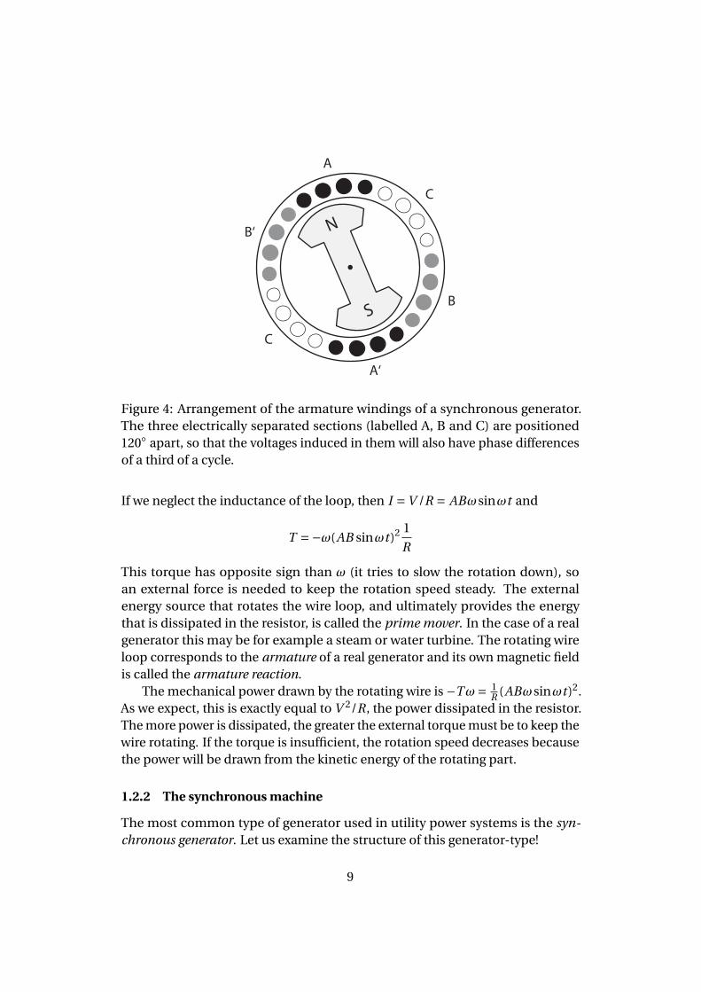
Figure 4: Arrangement of the armature windings of a synchronous generator.The three electrically separated sections (labelled A, B and C) are positioned120 apart, so that the voltages induced in them will also have phase differencesof a third of a cycle.

If we neglect the inductance of the loop, then I =V /R = ABωsinωt and

T =−ω(AB sinωt )2 1

R

This torque has opposite sign than ω (it tries to slow the rotation down), soan external force is needed to keep the rotation speed steady. The externalenergy source that rotates the wire loop, and ultimately provides the energythat is dissipated in the resistor, is called the prime mover. In the case of a realgenerator this may be for example a steam or water turbine. The rotating wireloop corresponds to the armature of a real generator and its own magnetic fieldis called the armature reaction.

The mechanical power drawn by the rotating wire is −Tω= 1R (ABωsinωt )2.

As we expect, this is exactly equal to V 2/R, the power dissipated in the resistor.The more power is dissipated, the greater the external torque must be to keep thewire rotating. If the torque is insufficient, the rotation speed decreases becausethe power will be drawn from the kinetic energy of the rotating part.

1.2.2 The synchronous machine

The most common type of generator used in utility power systems is the syn-chronous generator. Let us examine the structure of this generator-type!

9

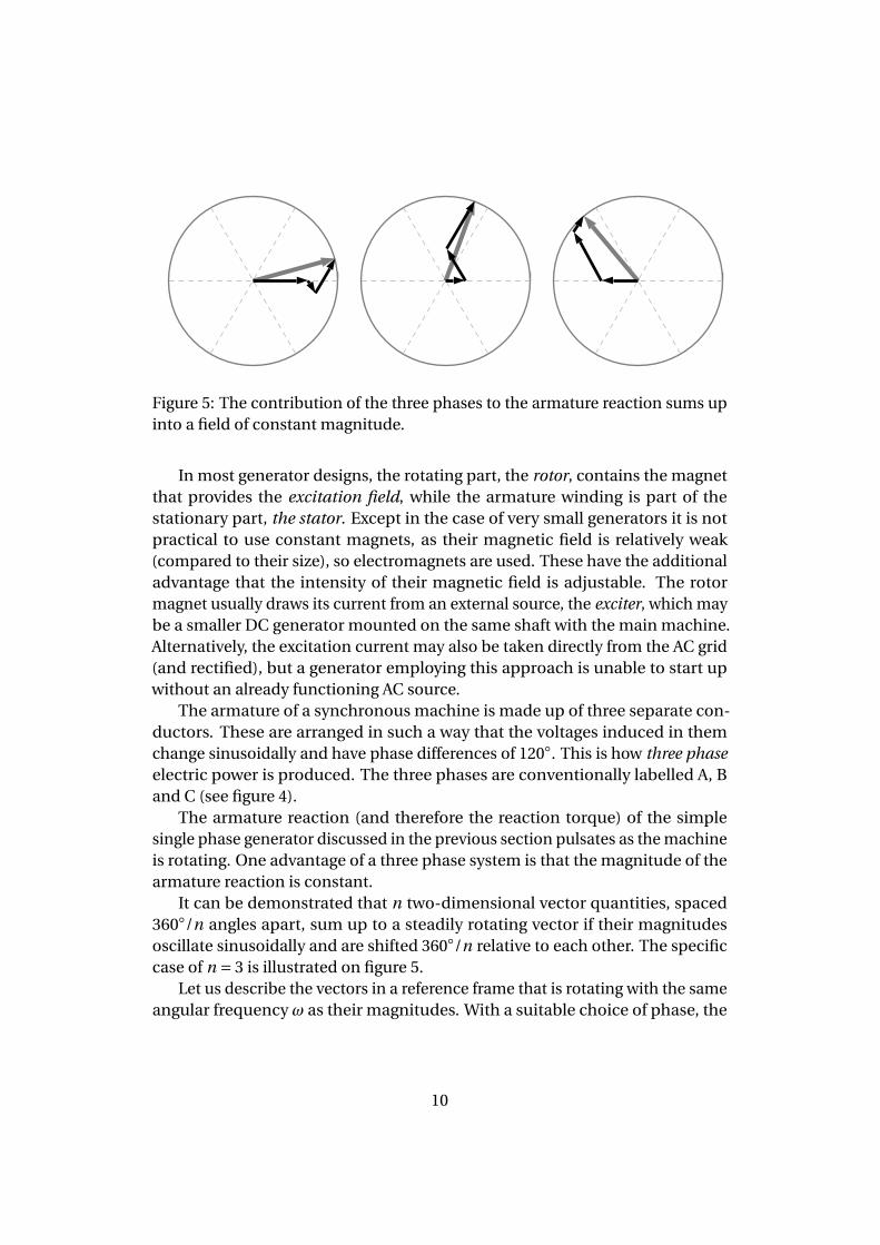
Figure 5: The contribution of the three phases to the armature reaction sums upinto a field of constant magnitude.

In most generator designs, the rotating part, the rotor, contains the magnetthat provides the excitation field, while the armature winding is part of thestationary part, the stator. Except in the case of very small generators it is notpractical to use constant magnets, as their magnetic field is relatively weak(compared to their size), so electromagnets are used. These have the additionaladvantage that the intensity of their magnetic field is adjustable. The rotormagnet usually draws its current from an external source, the exciter, which maybe a smaller DC generator mounted on the same shaft with the main machine.Alternatively, the excitation current may also be taken directly from the AC grid(and rectified), but a generator employing this approach is unable to start upwithout an already functioning AC source.

The armature of a synchronous machine is made up of three separate con-ductors. These are arranged in such a way that the voltages induced in themchange sinusoidally and have phase differences of 120. This is how three phaseelectric power is produced. The three phases are conventionally labelled A, Band C (see figure 4).

The armature reaction (and therefore the reaction torque) of the simplesingle phase generator discussed in the previous section pulsates as the machineis rotating. One advantage of a three phase system is that the magnitude of thearmature reaction is constant.

It can be demonstrated that n two-dimensional vector quantities, spaced360/n angles apart, sum up to a steadily rotating vector if their magnitudesoscillate sinusoidally and are shifted 360/n relative to each other. The specificcase of n = 3 is illustrated on figure 5.

Let us describe the vectors in a reference frame that is rotating with the sameangular frequency ω as their magnitudes. With a suitable choice of phase, the

10

vectors’ components are

vn = sin(ωt +2π

k

n

)·(cos

(ωt +2π

k

n

), sin

(ωt +2π

k

n

)), k = 1..n.

Summing the vectors up we get

n∑k=1

vn =n∑

k=1

(1

2sin

(2ωt +4π

k

n

),

1

2− 1

2cos

(2ωt +4π

k

n

))=

(0,

n

2

)+ 1

2

n∑k=1

(sin

(2ωt +4π

k

n

),−cos

(2ωt +4π

k

n

))︸ ︷︷ ︸

0

.

The second term is just a set of equally spaced vectors of the same lengths, whosesum is zero. The sum does not depend on ω, hence in the static reference frameit is a rotating vector of constant magnitude.

This result can be applied to the armature reaction of the synchronous gener-ator, which is called the stator field. This type of generator is called synchronousfor the very reason that the excitation field and stator field are rotating in accor-dance, in other words: they maintain a fixed position relative to each other. As aresult, the torque is also constant.

In situations when it is impractical to rotate the generator with the desirednetwork frequency (usually 50 Hz or 60 Hz), a rotor with four or more magneticpoles is used.

The induced voltage follows the magnetic flux with a phase lag of 90. Corre-spondingly, when the load is purely resistive, the stator field is perpendicular tothe rotor field. Otherwise it deviates from this position by an angle that is equal

stator field

rotor field

A.

C.B.

Figure 6: Relative position of the stator field and rotor field. A: Power factor ofunity. B: Lagging power factor. C: Leading power factor.

11

to the phase lag ϕ of the current (fig. 6). We should note that a purely resistiveload is not a realistic situation inasmuch as the generator itself has a non-zeroinductance. And since most loads are inductive too, a lagging power factor is themost common.

The torque acting on a magnetic dipole is the cross product of the dipole’smagnetic moment and the external field. Therefore the magnitude of the torqueon the rotor is determined by the perpendicular component of the stator field.The stator field is a function of the armature current, which in turn depends onthe load connected to the generator. As appliances are turned on and off, the loadchanges, so the torque must be adjusted continually to maintain equilibriumand keep the rotation speed constant. This is usually done by an automaticcontrol system, which is called the governor (fig. 8).

The induced electromotive force is determined by the rotation speed (whichis kept constant) and the magnitude of the rotor field. Assuming that the primemover can exert a great enough torque, while the rotor field and stator field areperpendicular, the voltage is constant, no matter how large the load is. But whenthe power factor differs from 1, the stator field has a component that is parallelto the rotor field, effectively changing the magnitude of the rotor field and theinduced voltage. A lagging power factor causes a reduction in voltage, a leadingpower factor causes an increase. This can be compensated for by changing theexcitation current.

1.2.3 Coupling of generators

When there are multiple generators in an AC system, all of them rotate at thesame angular frequency, and their output must have approximately the samephase at any time. It can be shown that if one of the generators speeds up, andits phase begins to get ahead of the others, the torque on its rotor will increase,preventing any further increase in the phase difference. Thus the generatorstend to be “locked” together.

When two generators are operating in parallel and there is a slight phasedifference, ϕ, between their output voltages, an electromotive force ∆V exists inthe “inner” circuit comprised by the two generators. Suppose that generator 2 islagging behind generator 1. As it is illustrated on figure 7, ∆V is ahead of the firstgenerator’s output voltage by approximately 90. It is a very good approximationto neglect the generators’ resistance compared to their inductive reactance, sothe current in the inner circuit, I (which is called the circulating current), has thesame phase as the output voltage of generator 1. Thus the circulating currentwill cause an increase in the perpendicular component of the stator field in thefirst generator, and a decrease in the second generator.

The slight phase angle that a generator has compared to the rest of the

12

V₁~

V₂~

ΔV~

I~

V₁~

V₂~

I~

φ

Figure 7: Two generators operating in parallel. When there is a phase differencebetween the electromotive forces of the two generators, the one which is aheadexperiences a greater torque due to the increased armature reaction.

network is called the power angle or voltage angle. It is directly related to thegenerator’s share of power production.

2 Power system control

Electrical generators are usually operated as part of a large interconnected net-work, the power grid. If one generator fails, in a large enough network theremaining generators can quickly fill newly created gap between power con-sumption and power production, and prevent an outage.

A group of generators which have AC connections between them form asynchronous area. As explained in the previous section, within such a network,every generator must rotate with the same frequency, and thus the networkfrequency is the same everywhere. Today, synchronous areas can be very large,and contain the power network of several countries. Examples of such largenetworks in Europe are the UCTE (Union for the Co-ordination of Transmissionof Energy), which encompasses most of mainland Europe, and NORDEL (NordicElectricity System), whose members are the Scandinavian countries.

Synchronous areas can be subdivided into control areas, which are controlledby a single company, the transmission system operator (TSO). The responsibilityof transmission system operators is to operate and maintain the electric gridin their area, and ensure that the system frequency does not deviate from a

13

Turbine Generator

Boiler

Feedback

Valve

ω−ω₀

50 Hz

stea

m fl

ow

Figure 8: The torque is continually adjusted to keep the system frequency ata constant value, usually 50 Hz or 60 Hz. For example, in the case of a steamturbine, the steam flow (which determines the torque exerted by the turbine) isadjusted using a valve.

prescribed value, which is 50.0 Hz in most of Europe.A difficulty with electric energy production is that electric energy cannot

be stored, except for very small quantities and short times. Therefore it mustbe produced at the same time at which it is consumed. The production mustmatch the consumption at every instant. This is no easy task—the power plantsneed to be continuously regulated to ensure that their power output matchesthe demand of the customers.

The control methods are based on the fact that when the balance betweenpower consumption and power production is upset, the system frequency startsto change. As it was shown in the previous section, when the load on a generatorincreases, the reaction torque becomes larger. If this change is not compensatedfor by increasing the driving torque, the turbine will start to slow down.

Because the total power consumption in a network cannot be measureddirectly (and efficiently), the balance is maintained by keeping the system fre-quency constant.

In the UCTE synchronous area, four levels of control are used (fig. 8), eachone working at a longer time-scale than the previous ones.

The primary control works at the level of individual generators. We shallstudy it in greater detail in section 2.1. Primary control restores the balanceof production and consumption in case of a disturbance. But it does not read-just the system frequency to the prescribed value. It merely ensures that the

14

Systemfrequency

Primarycontrol

Secodarycontrol

Tertiarycontrol

Timecontrol

free reserves

free reserves

restore normal operation

restore mean to match with UT

limit deviation

activate on long term

activate

take over

take over

Figure 9: Frequency control of a synchronous area.

frequency does not keep drifting away from the standard value when the bal-ance is upset. Figure 13A illustrates the behaviour of the system under primarycontrol—when there is a jump in power consumption, the frequency stabilisesat a new point, and stays constant afterwards. The difference between the newand old stable values is called the quasi-steady-state deviation.

It is called “quasi-steady-state” because on the characteristic time scale ofprimary control this deviation can be considered constant. The value of thesystem frequency is brought back to the prescribed value by the secondarycontroller. Secondary control is also automatic, but it is centralised: it works atthe level of control areas. Its function is to restore the frequency to the prescribedvalue of 50 Hz, and to restore power exchanges with the neighbouring controlareas to the scheduled values.

While every generator needs to have some kind of speed regulator (which isin fact the primary controller), not all of them participate in secondary control.Different generators can react to changes with different speeds, and have differ-ent ranges of power output where they can operate. Therefore some of them are

15

operated as base-load plants, i.e. they operate at a constant power output.Tertiary control functions at an even longer time scale than secondary con-

trol. Its role is to restore the set working point (power output) of generatorsparticipating in secondary control by redistributing the load between them or bystarting up additional generators. This may be done automatically or manually.

The final level of control, having the least impact on short time scales, is thetime control. The fictional time corresponding to system frequency is called thesynchronous time. According to UCTE regulations, synchronous time may notdeviate from the Coordinated Universal Time (UCT) by more than 30 seconds.This is ensured by measuring the time deviation each day (at 8 a.m. CET), andif it is greater than 20 seconds, setting the prescribed system frequency for thefollowing day 10 mHz higher or lower than 50 Hz. A deviation of 10 mHz fromthe prescribed 50 Hz causes a shift of 17.28 seconds in synchronous time duringa single day.

2.1 Practical governor models

In this section we shall examine some practical mechanisms used for speedgoverning, and derive simple mathematical models for them.

The principle behind any such governing mechanism is to compare therotation speed to a pre-determined value, and if there is a difference, makeadjustments to the torque driving the machine. There are several possibilities ofhow exactly these adjustments should be made in order to maintain the stabilityof the system. A few simple approaches are considered below.

2.1.1 The flyball governor

One of the simplest methods for regulating the rotation speed of machines isto exploit the centrifugal force. The centrifugal governor, also called the flyballgovernor, has already been in use as early as the 18th century. Its first use toregulate steam engines is attributed to James Watt himself.

The centrifugal governor consists of two heavy weights, called flyballs, thatare rotating together with the shaft (fig. 10). The flyballs are held together by aspring, but as they rotate, the centrifugal force pushes them apart. The faster therotation, the greater their distance from the axis becomes, and thus the angularvelocity is “converted” to a displacement parameter. This displacement can bemechanically transferred to a valve (for example, through a system of levers),and used to adjust the steam flow.

Let us make a simple, linearised model for this governor system! The inertiaof the flyballs is vanishingly small compared to the inertia of the turbine theyare coupled to. Therefore on the time scales where the rotation speed changes it

16

steam valve

flyball

displacement

Figure 10: The centrifugal governor. This simple device can be used to regu-late the steam flow with a valve (as shown on figure 8), and keep the networkfrequency constant.

is a good approximation to consider the governor system to be in equilibrium,i.e. the spring force and the centrifugal force are balanced at any time.

We shall denote the distance of the flyballs from the axis with r , and theelongation of the spring by x. Values at the standard operating point (when theangular velocity is the prescribed ω0) will be noted with a subscript 0, and thedeviations from them will be noted with a prime:

r = r0 + r ′ x = x0 +x ′

When the displacements are not very large, i.e. |r ′|¿ r0 etc., the relation betweenr ′ and x ′ can be approximated as r ′ =αx ′. It follows from the principle of energyconservation that when the centrifugal force is balanced by the spring, the twoforces are related as Fspring = r ′

x ′ Fc.f. =αFc.f.. (The infinitesimal work, F d x, doneat one end of a lever system must be equal to the work at the other end.)

The balance of forces can be written as

Fc.f. = m(ω0 +ω′)2(r0 + r ′) = 1

αk(x0 +x ′) = 1

αFspring.

m is the mass of the flyballs, and k is the spring constant. Let us expand theseexpressions and ignore those terms that are higher than first order in any of theprimed quantities:

mω20r0 +mω2

0r ′+2mω0r0ω′ = 1

αkx0 + 1

αkx ′.

17

Substituting r ′/α for x ′ and using the fact that the equation must hold for ω′ = 0,r ′ = x ′ = 0, we get (

mω20 −

k

α2

)r ′ =−2mω0r0ω

′.

It is a requirement that for a constant angular velocity the system must bestable, i.e. when r ′ is changed by a small amount, the resulting force imbalanceshould act to return it to its initial value. For ω′ = 0, this constraint leads tok/α2 > mω2

0. In other words, the spring must have a minimal stiffness for thesystem to be stable.

We have established that for relatively small deviations, ω′ is proportional tor ′ and x ′: ω′ =C · r ′ =αC ·x ′, where C is a positive constant.

The flyball mechanism can convert variations in rotation speed to displace-ment, but it cannot exert a force great enough to open or close a large valve.Therefore some force amplifier is must be used in practice, such as the hydraulicdevice illustrated on figure 11. This particular device does not simply enlarge adisplacement by a multiple, because for as long as the pilot valve is open, thepiston keeps moving. As a linear approximation we can regard the positionof the pilot valve, x, as directly determining the rate of change in the positiony of the piston: −(const.) · x = y . In other words this valve–piston system is amechanical integrator.

In order to be able to study this governor system in more detail, let us look athow the turbine behaves. If its moment of inertia isΘ, and the torque acting on

flow control valve

pilot valve

x

y

piston

pressure

Figure 11: Hydraulic mechanism (actuator) used to operate the flow controlvalve. The more the pilot valve is opened, the greater the force on the piston,therefore the input displacement (x) determines not the magnitude, but the rateof change of the output: y =−(const.) ·x.

18

it is T , then its motion is described by the equation

ωΘ= T.

This is called the swing equation. The torque is the difference of the drivingtorque, Td and the electrical reaction torque, Tr. The latter is depends on theelectrical load connected to the generator, and cannot be controlled. The drivingtorque must be constantly adjusted to balance the reaction torque and to correctany deviations from the prescribed system frequency. There is also a smalldamping torque, arising from various electrical and mechanical effects, whichincreases with the rotation speed. We shall use Tdamping = −Dω as a linearapproximation.

Now that we have all the pieces, let us put the equations together. The totaltorque is T = Td −Tr −Dω. For simplicity, let us assume that the electric loaddoes not change in time, so Tr is constant. The driving torque is determinedby the position of the steam-flow valve, so T =−Dω+C1 y + (const.), where C1

denotes a constant. Taking the derivative of this equation, we get T =−Dω+C1 y = −D d

d t (ω0 +ω′)−C2x. But x, the input to the hydraulic force-amplifier,is proportional to the deviation (ω′) from the preferred rotation velocity, soT =−Dω′−C3ω. Using the swing equation, we get

ω′Θ=−Dω′−C3ω′,

which (for C3 > 0) is the differential equation of a damped harmonic oscillator. Asmall disturbance of the rotation velocity dies off after a number of oscillations,no matter what the value of Tr is. But notice that the damping term in thisequation represents the natural damping of the rotor itself, and the governormechanism itself has no “built-in” damping.

The type of control described here is called integral control because thefeedback is through the time-integral of the regulated variable’s error.

2.1.2 Speed droop governor

The governor discussed in the previous section does not have very good stabilityproperties as it relies on the natural damping of the rotor. Better results can beachieved if the hydraulic integrator is converted to a displacement amplifier bymeans of a summing beam (a lever) that provides feedback to the pilot valvefrom the piston’s position (fig. 12). In this device the position of the pilot valveis the sum of the input displacement x and a constant multiple of the outputy . Its behaviour is described by the differential equation y =−(const.) · (βy + x).The steady state solution of this equation is y =−x/β, so we see that this deviceworks as a displacement amplifier. By making the feedback proportional to thefrequency-deviation, we got a proportional controller.

19

If the driving torque corresponding to y = 0 is Td0, and we ignore the damp-ing term, then the swing equation is

Θd

d t(ω0 +ω′) = Td0 + (const.) · y −Tr.

The steady state solution is Tr−Td0 = (const.) · y =−(const.) ·ω′. Hence this typeof governor does not keep the rotation speed constant. But it does limit thedeviation from the nominal value as the reaction torque changes.

The power output of a rotating machine is ω ·Tr. Since the relative changein rotation speed cannot be very large under normal operation, we can saythat the reaction torque is simply proportional to the power output. Thus therelationship between the power load and rotation speed of a generator is linear,as illustrated in figure 13A.

The slope of this curve on fig 13A is characteristic for every generator. It isusually expressed as the ratio of relative changes in rotation speed and poweroutput,

s =−ω′/ω0

P ′/P0(in %),

and is called the droop of the generator. In this formula P0 is the rated real poweroutput of the generator, while P ′ is the deviation from this value.

When there are several interconnected generators, the proportion in which aload increase is shared between them is determined by their droop values.

y

x

pressure

flow control valve

Figure 12: Hydraulic displacement-amplifier (servomechanism). A lever (the“summing beam”) functions as a feedback mechanism that limits the displace-ment of the piston. Unlike the hydraulic device of 11, this system has a steadystate. In the steady state, the piston position y is proportional to the inputdisplacement x.

20

P

Ω

A

5 10 15 20time

Ω'

B

Figure 13: A: The relationship between the power load of the generator and therotation speed when the speed droop governor is operating. B: Response ofthe speed droop governor to a sudden drop in power consumption: followingthe power drop at time 5, the rotation speed stabilises at a new, higher value.(Because this example is meant to illustrate the behaviour of this governor typeand because machines of different sizes have different reaction times, exact timeunits are not specified.)

3 Data analysis and simulations

In this section we shall analyse frequency and demand measurement data fromtwo synchronous areas. A simple model of a control area will be constructed,and studied using computer simulation. The results will be compared with themeasured data.

3.1 Data sources

Frequency measurement data was obtained from two sources: the UCTE, andthe National Grid Company (United Kingdom).

Real-time frequency data for the UCTE synchronous area is available onthe UCTE website [6]. A computer program was used to continuously monitorthe site and retrieve the data. The data has a time resolution of 2 seconds andfrequency resolution of 1 mHz.

The National Grid Company of the United Kingdom provides both frequencyand power consumption measurements [7]. The frequency data has a resolutionof 10 mHz and is updated every 15 seconds. The demand is given in megawattsand is updated every minute. However, National Grid’s data source—especiallytheir frequency measurements—proved to be much less reliable than UCTE’s.Data was usually unavailable for several short periods during a day, and measure-

21

ment times were often mismatched, thus further reducing the time resolution.Because of this we shall mainly work with the UCTE frequency measurements.

Let us plot the frequency and demand data for intervals of different lengths.Frequency variations for a weekday are plotted on fig. 18 for the UCTE networkand fig. 17 for the National Grid network. Note how UCTE operates its gridwithin stricter frequency bounds than National Grid. There are additional plotson which the data of a shorter period is magnified (figures 16, 19, and 20).

It is interesting to note that almost all big frequency jumps happen at sharphours. This is especially visible on fig. 18. We can verify this observation quan-titatively by calculating the standard deviation of the frequency values, andlooking at how it changes during a day. The results of this calculation are plottedon fig. 22. It is not surprising that most frequency jumps are at sharp hours,because our society functions by the 24-hour clock. Consumers tend to startand finish activities (and therefore turn on and turn off electric machines) atinteger hours; work hours start and end at sharp hours. The scheduling of powerexchanges is also done for hourly or half-hourly periods. But it is importantto note that these effects should be taken into consideration in the regulationof the electric network. At times when large frequency jumps are likely, moreregulating capacity is needed.

On shorter time scales there is no discernible order in the frequency fluctua-tions (figures 16, 19, and 20).

The distribution of the frequency values in the UCTE network is plottedon fig. 21. It can be seen that (in accordance with the regulations), the systemfrequency tends to stay within 100 mHz of the prescribed value of 50 Hz. Thehistogram was made using data from a number of time periods, approx. 25 daysin total.

The demand data from National Grid is plotted on figures 14, 15 and ??. Onthese plots, the most apparent feature is of course the daily variations, but if wezoom in to shorter time scales, comparable with 1 hour, the random fluctuationsbecome visible. Unfortunately the time resolution of the data is not good enoughto go to an even shorter time scale and make a comparison with the frequencyfluctuations.

3.2 Description of the model

Let us construct a simple model that can be used for numerical simulation offrequency variations in a synchronous area.

As discussed in section 1.2.3, under normal operating conditions all ma-chines in an interconnected AC grid are rotating with the same frequency. There-fore we shall use a single angular frequency, ω, for the complete control area.Notations will be used as follows: ω′ =ω−ω0 – the deviation from the prescribed

22

5 6 7 8 9 10 11 12 13 14 15 16 17 18 19 20 21 22 23 24 25 26 27 28 29

25

30

35

40

45

Day of month HApril, 2007L

Dem

and

HGW

L

Figure 14: Power demand variation during April, 2007 in the electric networkof the National Grid Company (United Kingdom). During weekends the topdemand is less than on weekdays. The period from the 6th to the 9th was aholiday (Good Friday to Easter Monday).

0 1 2 3 4 5 6 7 8 9 10 11 12 13 14 15 16 17 18 19 20 21 22 23 0

30

35

40

hour of day

Dem

and

HGW

L

Figure 15: Demand variation during one day (11th of April, 2007, Monday) in theNational Grid network. At this time scale the curve is dominated by the dailyvariations—power consumption is greater during the day than during the night.Random variations are only visible at shorter time scales. Frequency data for thesame day is plotted on fig. 17.

9 10 11 12

42.842.943.043.143.243.343.4

hour of day

Dem

and

HGW

L

Figure 16: A section of fig. 15, magnified. At this time scale the random changesare visible.

23

0 1 2 3 4 5 6 7 8 9 10 11 12 13 14 15 16 17 18 19 20 21 22 23 049 700

49 800

49 900

50 000

50 100

50 200

time Hhour of dayL

freq

uenc

yHm

HzL

11th of April, 2007, Monday

Figure 17: Frequency variations during the 11th of April, 2007, in the NationalGrid network. The frequency scale of this graph is the same as that of figure 18(UCTE frequency data), therefore they are directly comparable. Note how fre-quency control is less tight than in the UCTE grid. Spacing of horizontal lines is25 mHz.

24

0 1 2 3 4 5 6 7 8 9 10 11 12 13 14 15 16 17 18 19 20 21 22 23 049 900

49 950

50 000

50 050

50 100

freq

uenc

yHm

HzL

15th of March, 2007, Thursday

0 1 2 3 4 5 6 7 8 9 10 11 12 13 14 15 16 17 18 19 20 21 22 23 049 900

49 950

50 000

50 050

50 100

time Hhour of dayL

freq

uenc

yHm

HzL

16th of March, 2007, Friday

Figure 18: Frequency variations during two consecutive weekdays in the UCTEsynchronous area. Notice that most abrupt frequency changes happen at sharphours. This is partly because of the behaviour of consumers, and partly becausethe scheduling for power exchanges between adjacent control areas is made forhourly or half-hourly intervals. See also figure 22 on how standard deviation offrequency fluctuations is changing during a day.

15 15.25 15.5 15.75 1649 900

49 950

50 000

50 050

50 100

time Hhour of dayL

freq

uenc

yHm

HzL

Figure 19: Frequency variations during a one hour period (15th of March, 2007).

25

54 000 54 060 54 120 54 180 54 240 54 300 54 360 54 420 54 480 54 540 54 60049 900

49 950

50 000

50 050

50 100

time Hseconds elapsed since the start of the dayL

freq

uenc

yHm

HzL

Figure 20: Frequency variations during a ten minute period (15th of March, 2007).Time is in seconds elapsed since the start of the day, i.e. this is approximatelyfrom 15:00 to 15:10.

49 950 50 000 50 050 50 100f HmHzL

Figure 21: Distribution of frequency values in the UCTE area. The histogramwas made using data gathered during a 25-day period. It can be seen that thefrequency does not usually deviate from 50 Hz by more than 50 mHz.

26

0 1 2 3 4 5 6 7 8 9 10 11 12 13 14 15 16 17 18 19 20 21 22 23hour of day

10

15

20

25

30

35

40

DfHm

HzL

Figure 22: This plot was made by dividing days into 15-minute intervals, andcalculating the standard deviation of frequency values (∆ f ) for each interval.Each point on the graph represents one interval. The intervals are centredaround 0, 15, 30 and 45 minutes; e.g. an interval around 12 o’clock lasts from11:52:30 to 12:07:30. The data was averaged for 4 days. The vertical lines aredrawn at sharp hours.

Note how all large values of ∆ f occur at sharp hours (compare with fig. 18).Other than the peaks at sharp hours, there is no discernible daily variation in∆ f .

This graph is based on the frequency data from the UCTE network.

27

angular frequency; pi – the power output of the i th machine; d – the total powerdemand in the system;Θi – the inertial momentum of the i th machine.

Machines usually respond to control with some delay. This delay may becaused by several factors, for example, in the case of a steam turbine, re-heatingmight be necessary before the power output can be increased; or the servomech-anism that operates the steam-flow valve may respond with a noticeable delay.We shall take into consideration all these delay-effects by introducing a “controlvariable”, vi , for each generator. The control mechanism adjusts the variable vi ,but the actual power output follows vi with some delay. As a first order linearapproximation, we can use the equation pi = (vi −pi )/Ti , where Ti is a timeconstant. Obviously, the steady state solution is vi = pi .

For the control equation, we can use proportional-integral (PI) control (asdescribed in section 2.1). The proportional term represents primary control,while the integral term, which is responsible for bringing the frequency deviationω′ back to 0, represents secondary control. The control variable is set to thesum of these two terms: vi =−Gi ·

(ω′+ 1

τi

∫ω′ d t

). τi is the characteristic time

constant of secondary control, while Gi is a gain factor representing the “stiffness”of control.

Adding the only missing piece, the swing equation, we get the completesystem of differential equations describing our model:

ω′(t )

M︷ ︸︸ ︷ω0 ·

(∑iΘi

)=

(∑i

pi (t )

)−d(t )

vi =−Gi ·(ω′(t )+ ω′(t )

τi

)pi (t ) = vi (t )−pi (t )

Ti

Note that in the swing equation ω0 was substituted for ω. This is a goodapproximation since the relative frequency deviations are very small: ω′/ω0 ¿ 1.

Because there is a single angular frequency for the complete network, andbecause the moments of inertia appear only in the swing equation, the net-work can be considered to have a single parameter that characterises its inertia.ω0

∑i Θi can be replaced by a parameter M that scales linearly with the number

of generators.A computer program written in the C++ language was used to numerically

solve these equations for a power consumption that changes arbitrarily in time.Because the demand d(t ) may not vary smoothly, it was not possible to employ

28

higher order numerical integrators, so the straightforward Euler method wasused.

3.3 Simulation results

We are primarily interested in how the model behaves, and how it responds tochanges of parameters and different demand functions (d(t )). For this, it is notnecessary to use real physical units; to keep things simple, all parameters will begiven as numbers.

Changing parameter values is mathematically equivalent to choosing differ-ent units, so it is useful to fix the value of some of the parameters to eliminateany redundancy. In reality, the number of relevant parameters for this system isonly two. For the inertial parameter M a value of 1/generator will be used (it willbe numerically set to the number of generators). For the controller gains Gi , weshall use values around 1.0. Only the two time constants will be varied.

Also note that the swing equation contains the difference of the total produc-tion (

∑i pi ) and the demand d . The magnitude (as opposed to the derivative) of

these quantities does not appear at any other place in the equations (except theequation which relates vi to pi ). Therefore, provided that the initial values ofvi are the same as pi , the behaviour of the system does not change if the sameconstant is added to both d and

∑i pi . In other words, if we have a solution of

this system of equations for a particular d(t ) function, this solution can be trans-formed into a solution for another system with the demand function d(t )+d0

by simply adding constants to pi in such a way that∑

i pi is also increased by d0.For reasons of simplicity (and to avoid redundancy), the initial conditions willalways be set to pi = d = 0 for all i . This should not be interpreted as 0 demandand production, but as 0 deviation from a positive demand and production.

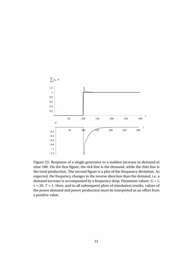
First, let us look at the how the model behaves when the demand is suddenlyincreased. The results of the simulation are plotted on figures 23 and 24. Asexpected, after the increase, the power output stabilises at the new value of d .The higher the delay factor the more time is needed for the oscillations to die off.

Now let us see what happens under the same load conditions as before whenthere is more than one generator. The power outputs of two generators areplotted on fig. 25. The generator with the quicker response (i.e. the one withthe smaller delay factor) takes the higher share of the final load. Otherwise theirbehaviour is similar in the sense that both power outputs oscillate at the samefrequency before stabilisation. In our model this is true for any number of gen-erators because there is a single angular frequency, and a single swing equationfor the complete system. No matter how many generators are there, and whatare their parameters, because of the frequency locking, all of them respond toa disturbance with oscillations of the same frequency, but perhaps different

29

amplitudes and damping factors. This system is not capable of producing ran-dom frequency fluctuations, even if all generators have different parameters.Therefore the source of the frequency fluctuations visible in measurement datamust lie in the short time-scale demand fluctuations.

We saw that in practice the power consumption changes randomly on smalltime scales. The simplest model for a randomly changing but continuous curveis the random-walk. We can use a random-walk curve to model the changes indemand, and see what frequency fluctuations arise in the system.

These simulations were run with approximately 100 generators. Generatorand control parameters were chosen randomly (with a uniform distribution)from intervals. The exact parameters for each run of the model are documentedin the figure captions. Since the secondary control is centralised, it is reasonableto assume that generators respond similarly to it, regardless of their type, so τi

were chosen from a narrow interval. The gains Gi were drawn from the interval0.5..2.0 for each run. The delay constants Ti were allowed to change over anorder of magnitude to reflect the differences between types.

As we expect, the production follows the demand, but it is smoothed outbecause of the finite response time of the control mechanism (fig. 26). A smallerdelay constant allows the system to follow the demand more precisely (fig. 28).Though this is not very apparent on the figures where the secondary control isstrong enough, on figure 29, where the effect of secondary control was reducedby giving τi large values, it can be seen that the frequency curve is very similarto the negative of the demand curve, but large variations are reduced on a longtime scale. This is in accordance with the linear relationship that exists betweenpower and frequency variations when proportional control is used.

Furthermore it can be observed that a larger number of generators can exerta tighter control over frequency. As we compare figures 26 and 27, we see thata tenfold reduction in the number of generators available for control increasesthe frequency variations by ten times.

Unfortunately the demand data at our disposal does not have a high enoughresolution to make it possible to compare frequency and demand fluctuations,and see a direct correlation.

But our second observation, namely that a larger number of controllers canexert a tighter control, could be used to assess the state of the power grid from thefrequency measurements. Figure 22 shows that—apart from the hourly peaks—the magnitude of frequency fluctuations is usually constant throughout the day.This means the there are sufficient control reserves at any time to maintainthe frequency within set bounds. However, we can expect that if the numberof machines participating in control is reduced, for example because some ofthe machines reach the bounds of their control range, then the magnitude offrequency fluctuations will increase.

30

50 100 150 200 250 300t

0.2

0.4

0.6

0.8

1

1.2

âi

pi, d

50 100 150 200 250 300t

-1.2

-1

-0.8

-0.6

-0.4

-0.2

Ω'

Figure 23: Response of a single generator to a sudden increase in demand attime 100. On the first figure, the tick line is the demand, while the thin line isthe total production. The second figure is a plot of the frequency deviation. Asexpected, the frequency changes in the inverse direction than the demand, i.e. ademand increase is accompanied by a frequency drop. Parameter values: G = 1,τ= 20, T = 1. Here, and in all subsequent plots of simulation results, values ofthe power demand and power production must be interpreted as an offset froma positive value.

31

50 100 150 200 250 300t

0.25

0.5

0.75

1

1.25

1.5

âi

pi, d

50 100 150 200 250 300t

-2

-1.5

-1

-0.5

0.5

Ω'

Figure 24: This is the same system as the one on fig. 23, but parameter valuesare different: G = 1, τ = 20, T = 5. A system with a higher delay-constant ismore unstable, i.e. it oscillates for a longer time before stabilisation, and theamplitude of oscillations is higher.

50 100 150 200 250 300t

0.2

0.4

0.6

0.8

p1, p2

Figure 25: Power output of two coupled generators under the same conditionsthat are described in the caption of fig. 23. Parameter values: G = 1 and τ= 10.One of the generators has a delay factor of T1 = 1, the other T2 = 3. The generatorwith the higher delay factor can responds a bit less quickly than the other one,therefore it takes the smaller share from the final load increase. Because thesystem has a single frequency, the two generators oscillate synchronously beforetheir power output is stabilised. This is true for any number of generators.

32

100 200 300 400 500t

-300

-200

-100

âi

pi, d

100 200 300 400 500t

-0.2

-0.1

0.1

0.2

0.3

Ω'

Figure 26: Behaviour of a 300-generator system. The demand function is gener-ated as a random-walk curve. Generator parameters are uniformly distributedin the following intervals: G = 0.5..2.0, τ= 30..40, T = 0.5..20.

On the first plot, the thin black curve is the power demand, while the thick greycurve is the total power production. On the second plot we see the frequencyvariation.

The production follows the demand curve closely, but with a slight delay.

33

100 200 300 400 500t

-125

-100

-75

-50

-25

25

âi

pi, d

100 200 300 400 500t

-2

-1

1

2

Ω'

Figure 27: This simulation was run with the same settings as the one whoseresults are plotted on fig. 26, but with only 30 generators. G = 0.5..2.0, τ =30..40, T = 0.5..20. Now the frequency deviations are 10 times greater. Thisis because fewer generators are only capable of proportionally smaller totalincrease/decrease in power output during a fixed amount of time.

34

100 200 300 400 500t

50

100

150

200

âi

pi, d

100 200 300 400 500t

-0.6

-0.4

-0.2

0.2

0.4

Ω'

Figure 28: Behaviour of a 100-generator system with the following parameters:G = 0.5..2.0, τ= 30..40, T = 0.5..5. Due to the smaller delay factors, the demandcurve is now more closely followed by the production curve.

35

100 200 300 400 500t

50

100

150

200

250

300

âi

pi, d

100 200 300 400 500t

-1.4-1.2-1-0.8-0.6-0.4-0.2

Ω'

Figure 29: Behaviour of a 100-generator system with the following parameters:G = 0.5..2.0, t au = 200..250, T = 0.5..5. Using large values for τ means havinga very slow (and “weak”) integral control (secondary control), so the dominantbehaviour is that of the proportional (primary) control.

The most striking difference between this figure and fig. 28 is that the fre-quency varies more loosely. In fact, the frequency curve mirrors the demandcurve. This is in accordance with the linear relationship between the frequencyand power deviations that we have derived for proportional control in sec. 2.1.2

36

4 Summary

The purpose of power system control is to maintain the delicate balance ofpower production and power consumption. This is necessary because largequantities of electric energy cannot be stored. Therefore electric power must betransmitted to the consumers as soon as it is produced.

It is not possible to measure the difference between power production andpower consumption directly, so power generation control is achieved throughmeasurement of another related parameter, the frequency of the alternatingcurrent. When the demand exceeds the production in a network, the frequencystarts to fall. The deviation of the frequency from a set value can be used asfeedback to adjust the power production and ensure that balance is maintained.In fact, power system control means ensuring that the system frequency doesnot deviate from a prescribed value.

Under normal operation the frequency is allowed to fluctuate only betweencertain bounds, which are set in the regulations of the system operator. Thiswork investigates the cause of these fluctuation, and explores the possibilities touse frequency measurements for a better system-level control.

The behaviour of a regulated network of interconnected generators wasstudied with computer simulations, and the results were compared with highresolution frequency measurements from two different power networks.

It has been found that the control system of generators does not producerandom fluctuations by itself. Instead, the frequency variations reflect the shorttime-scale fluctuations of power demand. However, the properties of frequencyfluctuations do depend on the state of generators participating in frequencycontrol, therefore it is possible to assess the state of the network from frequencymeasurements.

37

Bibliography

[1] P. M. Anderson and A. A. Fouad, Power System Control and Stability (IEEEPress, Wiley Interscience, 2003)

[2] Alexandra von Meier, Electric Power Systems: A Conceptual Introduction(IEEE Press, Wiley Interscience, 2006)

[3] UCTE Operation Handbook, final version 2.5/24.06.2004, available fromhttp://www.ucte.org/

[4] A villamosenergia-rendszer szabályozása, available from the HungarianTransmission System Operator Company (MAVIR),http://www.mavir.hu/

[5] Remus Fetea, Reactive power: A strange concept?, Physics Teaching in Engi-neering Education 2000

[6] Real-time frequency data for the UCTE grid is available on the UCTE mainpage: http://www.ucte.org/

[7] National Grid real-time operational data is available from the websitehttp://www.nationalgrid.com/uk/Electricity/Data/

38