Free-Form Sketching of Self-

Sketch-Based Interaction

50 January/February 2007 Published by the IEEE Computer Society 0272-1716/07/$20.00 © 2007 IEEE

S ketching interfaces to 3D object model-ing facilitate 3D object reconstruction

from a 2D drawing provided by a designer. Igarashipresented the Teddy silhouette-based sketching sys-tem, which has a simple, intuitive interface.1 Follow-up research has mainly focused on the representationissue for the resulting 3D objects, as given in recentwork: variational implicit surfaces2 and other forms ofimplicit surfaces.3

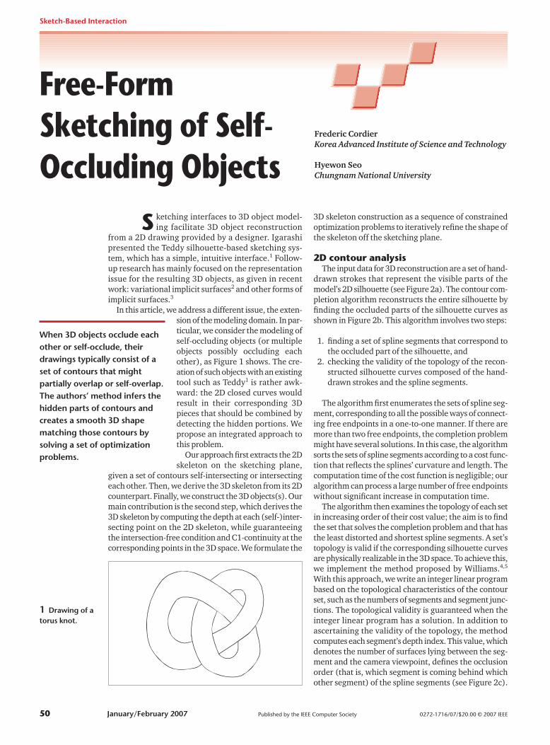
In this article, we address a different issue, the exten-sion of the modeling domain. In par-ticular, we consider the modeling ofself-occluding objects (or multipleobjects possibly occluding eachother), as Figure 1 shows. The cre-ation of such objects with an existingtool such as Teddy1 is rather awk-ward: the 2D closed curves wouldresult in their corresponding 3Dpieces that should be combined bydetecting the hidden portions. Wepropose an integrated approach tothis problem.

Our approach first extracts the 2Dskeleton on the sketching plane,

given a set of contours self-intersecting or intersectingeach other. Then, we derive the 3D skeleton from its 2Dcounterpart. Finally, we construct the 3D objects(s). Ourmain contribution is the second step, which derives the3D skeleton by computing the depth at each (self-)inter-secting point on the 2D skeleton, while guaranteeingthe intersection-free condition and C1-continuity at thecorresponding points in the 3D space. We formulate the

3D skeleton construction as a sequence of constrainedoptimization problems to iteratively refine the shape ofthe skeleton off the sketching plane.

2D contour analysisThe input data for 3D reconstruction are a set of hand-

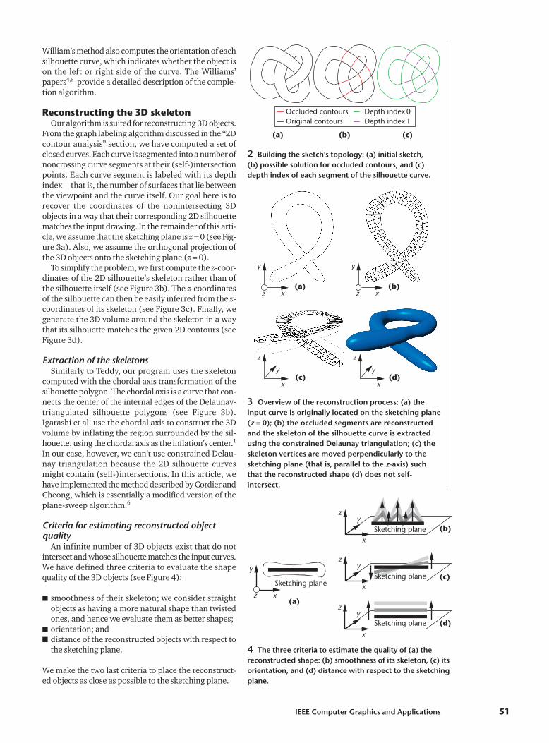
drawn strokes that represent the visible parts of themodel’s 2D silhouette (see Figure 2a). The contour com-pletion algorithm reconstructs the entire silhouette byfinding the occluded parts of the silhouette curves asshown in Figure 2b. This algorithm involves two steps:

1. finding a set of spline segments that correspond tothe occluded part of the silhouette, and

2. checking the validity of the topology of the recon-structed silhouette curves composed of the hand-drawn strokes and the spline segments.

The algorithm first enumerates the sets of spline seg-ment, corresponding to all the possible ways of connect-ing free endpoints in a one-to-one manner. If there aremore than two free endpoints, the completion problemmight have several solutions. In this case, the algorithmsorts the sets of spline segments according to a cost func-tion that reflects the splines’ curvature and length. Thecomputation time of the cost function is negligible; ouralgorithm can process a large number of free endpointswithout significant increase in computation time.

The algorithm then examines the topology of each setin increasing order of their cost value; the aim is to findthe set that solves the completion problem and that hasthe least distorted and shortest spline segments. A set’stopology is valid if the corresponding silhouette curvesare physically realizable in the 3D space. To achieve this,we implement the method proposed by Williams.4,5

With this approach, we write an integer linear programbased on the topological characteristics of the contourset, such as the numbers of segments and segment junc-tions. The topological validity is guaranteed when theinteger linear program has a solution. In addition toascertaining the validity of the topology, the methodcomputes each segment’s depth index. This value, whichdenotes the number of surfaces lying between the seg-ment and the camera viewpoint, defines the occlusionorder (that is, which segment is coming behind whichother segment) of the spline segments (see Figure 2c).

When 3D objects occlude eachother or self-occlude, theirdrawings typically consist of aset of contours that mightpartially overlap or self-overlap.The authors’ method infers thehidden parts of contours andcreates a smooth 3D shapematching those contours bysolving a set of optimizationproblems.

Frederic Cordier Korea Advanced Institute of Science and Technology

Hyewon SeoChungnam National University

Free-FormSketching of Self-Occluding Objects

1 Drawing of atorus knot.

William’s method also computes the orientation of eachsilhouette curve, which indicates whether the object ison the left or right side of the curve. The Williams’papers4,5 provide a detailed description of the comple-tion algorithm.

Reconstructing the 3D skeletonOur algorithm is suited for reconstructing 3D objects.

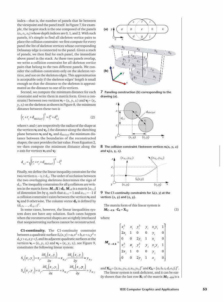
From the graph labeling algorithm discussed in the “2Dcontour analysis” section, we have computed a set ofclosed curves. Each curve is segmented into a number ofnoncrossing curve segments at their (self-)intersectionpoints. Each curve segment is labeled with its depthindex—that is, the number of surfaces that lie betweenthe viewpoint and the curve itself. Our goal here is torecover the coordinates of the nonintersecting 3Dobjects in a way that their corresponding 2D silhouettematches the input drawing. In the remainder of this arti-cle, we assume that the sketching plane is z � 0 (see Fig-ure 3a). Also, we assume the orthogonal projection ofthe 3D objects onto the sketching plane (z � 0).

To simplify the problem, we first compute the z-coor-dinates of the 2D silhouette’s skeleton rather than ofthe silhouette itself (see Figure 3b). The z-coordinatesof the silhouette can then be easily inferred from the z-coordinates of its skeleton (see Figure 3c). Finally, wegenerate the 3D volume around the skeleton in a waythat its silhouette matches the given 2D contours (seeFigure 3d).

Extraction of the skeletons Similarly to Teddy, our program uses the skeleton

computed with the chordal axis transformation of thesilhouette polygon. The chordal axis is a curve that con-nects the center of the internal edges of the Delaunay-triangulated silhouette polygons (see Figure 3b).Igarashi et al. use the chordal axis to construct the 3Dvolume by inflating the region surrounded by the sil-houette, using the chordal axis as the inflation’s center.1

In our case, however, we can’t use constrained Delau-nay triangulation because the 2D silhouette curvesmight contain (self-)intersections. In this article, wehave implemented the method described by Cordier andCheong, which is essentially a modified version of theplane-sweep algorithm.6

Criteria for estimating reconstructed objectquality

An infinite number of 3D objects exist that do notintersect and whose silhouette matches the input curves.We have defined three criteria to evaluate the shapequality of the 3D objects (see Figure 4):

■ smoothness of their skeleton; we consider straightobjects as having a more natural shape than twistedones, and hence we evaluate them as better shapes;

■ orientation; and ■ distance of the reconstructed objects with respect to

the sketching plane.

We make the two last criteria to place the reconstruct-ed objects as close as possible to the sketching plane.

IEEE Computer Graphics and Applications 51

2 Building the sketch’s topology: (a) initial sketch, (b) possible solution for occluded contours, and (c)depth index of each segment of the silhouette curve.

(a) (c)(b)

Depth index 0 Depth index 1

Occluded contours Original contours

3 Overview of the reconstruction process: (a) theinput curve is originally located on the sketching plane(z � 0); (b) the occluded segments are reconstructedand the skeleton of the silhouette curve is extractedusing the constrained Delaunay triangulation; (c) theskeleton vertices are moved perpendicularly to thesketching plane (that is, parallel to the z-axis) suchthat the reconstructed shape (d) does not self-intersect.

(a)

(c) (d)

(b)

y

xz

z

y

x

y

xz

z

y

x

Sketching plane

Sketching plane

Sketching plane

(a)

zy

x

Sketching plane

zy

x

zy

x

(b)

(c)

(d)

z

y

x

4 The three criteria to estimate the quality of (a) thereconstructed shape: (b) smoothness of its skeleton, (c) itsorientation, and (d) distance with respect to the sketchingplane.

Representing the skeletonAs we assign z-coordinates to the skeleton, we evalu-

ate the skeleton curve’s smoothness, which we can mea-sure by its curvature and torsion energies. Intuitivelyspeaking, the curvature energy measures the degree towhich the curve is bent, and the torsion is a measure forthe curve’s nonplanarity. Unfortunately, these two ener-gy terms are nonlinear7 and can complicate the prob-lem of optimization. Our solution is to represent theskeleton curves with a piecewise quadratic surface; byusing the approximation of the quadratic surface’s bend-ing energy,7 the energy terms become linear.

As Figure 5 shows, each edge vi, vj is associated witha quadratic surface of the form Sk(x, y) � ak.x2 � bk.x �ck.y2 � dk.y � ek.x.y � fk. This surface passes through thetwo vertices vi and vj, and is perpendicular to ni and nj

at the vertices vi and vj respectively. For each vertex vi,the variables (xi, yi) are the position coordinates on thesketching plane; the z-coordinates (zi) and normal coor-dinates (xN,i, yN,i) are the unknown variables of our recon-struction problem. Roughly speaking, the z-coordinatesand normal coordinates are related, respectively, to thebending and torsion deformations of the skeleton curve.Two quadratic surfaces connected to the same vertex vi

are C1-continuous at the point (xi, yi)—that is, they havethe same z-coordinate zi and normal ni vector at thatpoint.

By choosing the piecewise quadratic surface repre-sentation (see Figure 6), we obtain the curvature ener-

gy as a convex quadratic function of its coefficients,assuming the slight bending within the surface. Theminimization of such a function can be solved linearly.In addition, the curvature energy of the piecewise qua-dratic surface provides an estimation of both the torsionand bending energies of the skeleton curve.

A C1-continuity constraint is required to have smoothdeformation at the quadratic surfaces’ junction, as theskeleton bends. Intuitively speaking, the C1-continuitypropagates the bending and the torsion deformationalong the skeleton curves. As a vertex moves away fromthe sketching plane, the two surfaces adjacent to thisvertex will bend smoothly with the C1-continuity con-straint. Computing the curvature energy of these sur-faces provides us with a simple way to estimate theskeleton curve’s smoothness.

Formulating the shape reconstruction as a leastsquares problem

To compute the 2D skeleton’s position in the 3D space,we find the z-location zi and the normal coordinates (xN,i,yN,i) at the skeleton vertices vi � (xi, yi) that are the solu-tion of a least squares problem defined by an objectivefunction and a set of constraints. The objective function’spurpose is to estimate the quality of the reconstructedobjects, the inequality constraints prevent the objectswhose silhouettes overlap in 2D from intersecting eachother, and the equality constraints maintain the C1-con-tinuity between adjacent surfaces. Thus, we solve for anoptimization problem of the following form:

(1)

where X � (z0, xN, 0, yn, 0, … zm�1, xN, m�1, yn, m�1)T, with mbeing the number of skeleton vertices. Utotal denotes thematrix of the objective function for evaluating the qual-ity of the reconstructed models; MC1 is the matrix ofequality constraints for the C1-continuity, and Mcoll isthe matrix of the inequality constraints for preventingself-intersections.

Linear inequality constraints for the colli-sions. Since we don’t want the reconstructed shapesintersecting in 3D, special care must be taken to keepsome minimal distance between shapes whose 2D pro-jected images on the sketching plane overlap. We do soby placing a set of inequality constraints on the z-coordi-nates of skeleton vertices. First, we identify all pairs ofskeleton vertices for which the constraint must bedefined. Our approach makes use of the paneling con-struction by Williams.4 The paneling consists of creatinga set of 2D panels (or regions) on the sketching plane.Each panel is the projected image on the sketching planeof a region of the 3D shape, and is delimited by a set ofconnected segments of the close curves obtained fromthe contour completion step, as discussed previously. Fig-ure 7 shows an example of such paneling construction.

The paneling construction of a set of shapes whoseprojected images overlap on the sketching plane makesa stack of panels, each panel being assigned a depth

minX

z

XX

X dU

M

Mtotalcoll

subject to C10⋅ =

≥

⎧⎨⎪

⎩⎪


52 January/February 2007

5 A skeleton edge connecting vi to vj is associated witha quadratic surface Sk passing through vi and vj andwhose normal vectors are ni at vi and Nj at vj.

Sk

vj

vi

n

zy

x

i

n j

–xN,j–yN,j

1

–xN,i–yN,i

1

xiyizi

xjyjzj

6 The piecewise polynomial surface associated withthe skeleton: a polynomial surface Sk is associated witheach pair of connected vertices vi and vi � 1; two polyno-mial surfaces Sk and Sk � 1 are C1-continuous at theircommon vertex vi.

v0

v1 v2 v3

S0

S 1

S2

Sketching plane

0n

1n 2n3n

z

yx

index—that is, the number of panels that lie betweenthe viewpoint and the panel itself. In Figure 7, for exam-ple, the largest stack is the one composed of the panels(e0, e1, e2) whose depth indices are 0, 1, and 2. With suchpanels, it’s simple to find all skeleton vertice pairs toplace the collision constraint: we first compute for everypanel the list of skeleton vertices whose correspondingDelaunay edge is connected to the panel. Given a stackof panels, we then find for each panel, the immediateabove panel in the stack. As these two panels overlap,we write a collision constraint for all skeleton verticepairs that belong to the two different panels. We con-sider the collision constraints only on the skeleton ver-tices, and not on the skeleton edges. This approximationis acceptable only if the skeleton edges’ length is smallenough so that the distance to the skeleton is approxi-mated as the distance to one of its vertices.

Second, we compute the minimum distance for eachconstraint and write them in matrix form. Given a con-straint l between two vertices vi � (xi, yi, zi) and vj � (xj,yj, zj) on the skeleton as shown in Figure 8, the minimumdistance between these two is

(2)

where ri and rj are respectively the radius of the shape atthe vertices vi and vj, ll the distance along the sketchingplane between vi and vj, and dMinSurf the minimum dis-tance between the boundaries of the reconstructedshapes; the user provides the last value. From Equation 2,we then compute the minimum distance along the z-axis for vertices vi and vj:

Finally, we define the linear inequality constraint for thetwo vertices zi � zj � dz,l. The order of occlusion betweenthe two overlapping skeletons determines the sign ofdz,l. The inequality constraints for all q collisions are writ-ten in the matrix form: McollX � dz. Mcoll is a matrix [a3.i,l]of dimension 3m by q, such that a3.i,l � 1 and a3.i,l � �1 ifa collision constraint l exists between the vertices vi andvj and 0 otherwise. The column vector dz is defined by(dz,0, …, dz,q�1)T.

In some cases, however, the linear inequalities sys-tem does not have any solution. Such cases happenwhen the reconstructed shapes are so tightly interlacedthat nonpenetrating surfaces cannot be reconstructed.

C1-continuity. The C1-continuity constraintbetween a quadratic surface Sk(x, y) � ak.x2 � bk.x � ck.y2 �dk.y � ek.x.y � fk and its adjacent quadratic surfaces at thevertices vi � (xi, yi, zi) and vj � (xj, yj, zj), see Figure 9,constitutes the following linear system:

The matrix form of this linear system isMC�X,k � Ck � Xi,j (3)

where

and Xi,j � [zi xN,i yN,i zj xN,j yN,j]T and Ck � [ak bk ck dk ek fk]T.The linear system is rank deficient, and it can be eas-

ily shown that the last row R5 of the matrix MC�X,k is a

MC X k→ =

,

x x y y x y

x y

y x

x

i i i i i i

i i

i i

j

2 2

2

1

2 1 0 0 0

0 0 2 1 0

xx y y x y

x y

y x

j j j j j

j j

j j

2 1

2 1 0 0 0

0 0 2 1 0

⎡

⎣

⎢⎢⎢⎢⎢⎢⎢⎢⎢⎢

⎤⎤

⎦

⎥⎥⎥⎥⎥⎥⎥⎥⎥⎥S x y z

S x y

xx

S x y

yk i i ik i i

N ik i i, ,

,,

,,( ) =

∂ ( )∂

=∂ ( )

∂==

( ) =∂ ( )

∂=

∂

y

S x y zS x y

xx

S x

N i

k j j j

k j j

N j

k j

,

,, ,

,,

, yy

yy

j

N j

( )∂

=,

d r r d lz l i j MinSurf i.

= + +( ) −2

2

r r d l di j MinSurf l z l+ +( ) = +

22 2

,


7 Paneling construction (b) corresponding to thedrawing (a).

a0

d0

11

2

1 1

1

c0

g 0

f 0

i 0

j 0

b0 e0 h0 k0

b

f

e

e

g h

a b

c

d

e

f

g

i

j

h k

(b)

(a)

z

y

x

z

y

x

8 The collision constraint l between vertices vi(xi, yi, zi)and vj(xj, yj, zj).

x

z

z i

dz,l

ri

z j

(xi ,yi) (xj ,yj)

dMinSurf

y

rj

9 The C1-continuity constraints for Sk(x, y) at the vertices (xi, yi) and (xj, yj).

(xN,i ,yN,i ) (xN,j ,yN,j)

Sk(x,y)

x

z

z j

z i

(xi ,yi) (xj ,yj)y

linear combination of the other five rows, R0, …,R4, asin R5 � mk,0R0 � mk,1R1 � mk,2R2 � mk,3R3 � mk,4R4, where

As Xi,j is linearly related to MC�X,k as shown in Equation3, it follows that the similar linear dependency existsamong the elements of Xi,j: mk,0zi � mk,1xN,i � mk,2yN,i �mk,3zj � mk,4xN,j � yN,j � 0. Combining this linear constraintfor every surface, we write: MC1 � X � 0 where

with mk,0 � (mk,0, mk,1, mk,2) and mk,1 � (mk,3, mk,4, �1).

Curvature energy. A common approximation ofthe curvature energy of a thin plate s(x, y) under slightbending7 is

The constant D is the Young’s modulus (elasticitycoefficient of the plate) and v the Poisson’s ratio. In prac-tice, the Poisson’s ratio varies from 0 to 1/2. In this arti-cle, we use D � 2 and v � 1/2, and the approximatedcurvature energy of a quadratic polynomial surface Sk(x, y) associated with an edge (vi, vj), vi � (xi, yi), vj �(xj, yj), is

(4)

where

Equation 4 can be rewritten in the matrix form

where

Since Ecurv,k has a convex quadratic polynomial form, the coefficients ak, ck, and ek, minimizing this objective can be computed by solving the least squaresproblem:8

(5)

where the matrix

is computed by the Cholesky factorization of H. Clearly,working with the approximated curvature energy is lessexpensive than working with that of exact form, whichinvolves nonlinear terms.7

Now that we have found the curvature-energy objec-tive function using the quadratic coefficients Ck, werewrite it as a function of skeleton variables Xi,j so thatthe curvature energy term is seamlessly integrated intothe global optimization problem as in Equation 1. Ck

and Xi,j are linearly related from Equation 3; unfortu-nately, the matrix MC�X,k is rank deficient and cannotbe directly inverted. We therefore compute a matrixMX�C,k such that Ck � MX�C,kXi,j is a solution to the cur-vature minimizing problem of Equation 5 and a solu-tion to the linear system as in Equation 3. The“Computing the Matrix MX�C,k” sidebar describes thecomputation of this matrix. The objective function ofcurvature energy as a function of Xi,j is given by

(6)

where

Combining the objective function in Equation 6 forevery surface, we write:

(7)

where Ucurv is filled with lkU'MX�C,k for k � 0,…n � 1,n being the number of edges.

Orientation of the skeleton. The second criteri-on to evaluate the quality of the reconstructed shape isthe minimization of the orientation angle of its skeletonwith respect to the sketching plane (z � 0).

minX

XUcurv

U ' =

⎡

⎣

⎢⎢⎢⎢

⎤

⎦

⎥⎥⎥⎥

2 0 1 0 0 0

0 0 3 0 0 00 0 0 0 1 0

min ',

,X i ji,j

XU MX C k→

U =

⎡

⎣

⎢⎢⎢⎢

⎤

⎦

⎥⎥⎥⎥

2 1 0

0 3 00 0 1

min ( ), ,a c e k k k

T

k k k

a c eU ⋅

H =

⎡

⎣

⎢⎢⎢

⎤

⎦

⎥⎥⎥

4 2 02 4 00 0 1

E l a c e a c ecurv k k k k k k k k

T

,= ( ) ( )2 H

l x x y yk j i j i2

2 2= −( ) + −( )

E l a c e a ccurv k k k k k k k,

= + + +( )2 2 2 24 4 4

E

D s

x

s

y

v

s

curv=

∂∂

+ ∂∂

⎛

⎝⎜

⎞

⎠⎟ −

⎛

⎝⎜⎜

−( ) ∂

∫∫2

2 1

2

2

2

2

2ss

x

s

y

sx y

dxdy∂

∂∂

− ∂∂ ∂

⎛

⎝⎜

⎞

⎠⎟

⎛

⎝

⎜⎜

⎞

⎠

⎟⎟

⎞

⎠

⎟⎟⎟

2

2

2

22

MC

0,0 0,1

1,0 1,1

0 0 0 0 0

0 0 0 0 0

0 0 00

1=

m m

m m

�

�

� � � � �� mm m

m m

j j

n n

,0 ,1

,0

0 0

0 0 00 0 0 0

�

� � � � ��

,1

⎡

⎣

⎢⎢⎢⎢⎢⎢⎢⎢⎢⎢

⎤

⎦

⎥⎥⎥⎥⎥⎥⎥⎥⎥

my y

mx x

y ym

m

ki j

k

i j

i jk

k

, , ,

,

, ,0 1 2

21=

−= −

−( )−

= −,

33 4

2= −−

= −−( )−y y

mx x

y yi j

k

i j

i j

, and,



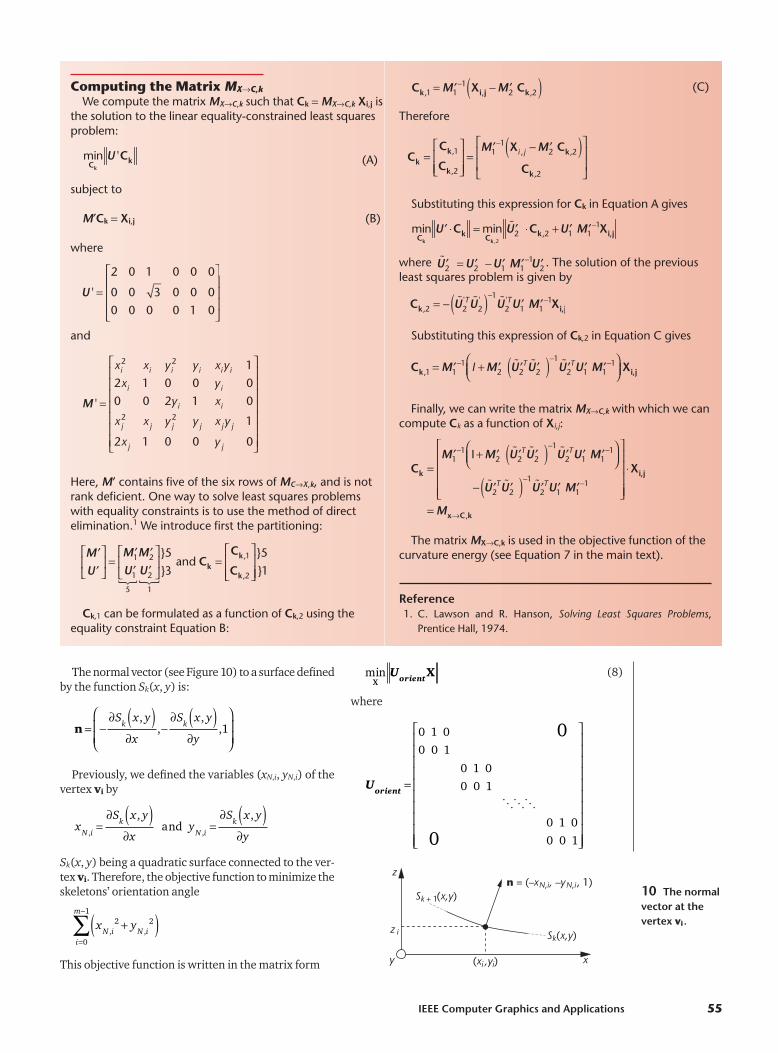
The normal vector (see Figure 10) to a surface definedby the function Sk(x, y) is:

Previously, we defined the variables (xN,i, yN,i) of thevertex vi by

Sk(x, y) being a quadratic surface connected to the ver-tex vi. Therefore, the objective function to minimize theskeletons’ orientation angle

This objective function is written in the matrix form

(8)

where

Uorient

=

0 1 00 0 1

0 1 00 0 1

0

0

0

��1 0

0 0 1

⎡

⎣

⎢⎢⎢⎢⎢⎢⎢⎢⎢⎢

⎤

⎦

⎥⎥⎥⎥⎥⎥⎥⎥⎥⎥

minX

Uorient

X

x yN i N i

i

m

, ,2 2

0

1

+( )=

−

∑

xS x y

xy

S x y

yN ik

N ik

, ,

, ,=

∂ ( )∂

=∂ ( )

∂and

n = −∂ ( )

∂−

∂ ( )∂

⎛

⎝⎜⎜

⎞

⎠⎟⎟

S x y

x

S x y

yk k

,,

,,1


10 The normalvector at thevertex vi.

n = (–xN,i, –yN,i, 1)Sk + 1(x,y)

Sk(x,y)

x

z

z i

(xi ,yi)y

Computing the Matrix MX�C,k

We compute the matrix MX�C,k such that Ck � MX�C,k Xi,j isthe solution to the linear equality-constrained least squaresproblem:

(A)

subject to

M�Ck � Xi,j (B)

where

and

Here, M’ contains five of the six rows of MC�X,k, and is notrank deficient. One way to solve least squares problemswith equality constraints is to use the method of directelimination.1 We introduce first the partitioning:

Ck,1 can be formulated as a function of Ck,2 using theequality constraint Equation B:

(C)

Therefore

Substituting this expression for Ck in Equation A gives

where . The solution of the previousleast squares problem is given by

Substituting this expression of Ck,2 in Equation C gives

Finally, we can write the matrix MX�C,k with which we cancompute Ck as a function of Xi,j:

The matrix MX�C,k is used in the objective function of thecurvature energy (see Equation 7 in the main text).

Reference1. C. Lawson and R. Hanson, Solving Least Squares Problems,

Prentice Hall, 1974.

Ck =′M1−1 I + ′M2

� ′U2T � ′U2( )−1 � ′U2

T ′U1 ′M1−1⎛

⎝⎜⎞⎠⎟

− � ′U2T � ′U2( )−1 � ′U2

T ′U1 ′M1−1

⎡

⎣

⎢⎢⎢⎢

⎤

⎦

⎥⎥⎥⎥

⋅Xi,j

= Mx→C,k

Ck ,1 = ′M1−1 I + ′M2

� ′U2T � ′U2( )−1 � ′U2

T ′U1 ′M1−1⎛

⎝⎜⎞⎠⎟

Xi,j

Ck ,2 = − �U2'T �U2

'( )−1 �U2'T ′U1 ′M1

−1Xi,j

� ′U2 = ′U2 − ′U1 ′M1−1 ′U2

minCk

′U ⋅Ck = minCk ,2

� ′U2 ⋅Ck ,2 + ′U1 ′M1−1Xi,j

Ck =Ck ,1

Ck ,2

⎡

⎣⎢⎢

⎤

⎦⎥⎥

=′M1−1 Xi ,j − ′M2 Ck ,2( )

Ck ,2

⎡

⎣

⎢⎢

⎤

⎦

⎥⎥

Ck ,1 = ′M1−1 Xi,j − ′M2 Ck ,2( )

′M

′U

⎡

⎣⎢

⎤

⎦⎥ =

′M1

′U1

⎡

⎣⎢

5�

′M2

′U2

⎤

⎦⎥

1�

}5

}3 and Ck =

Ck ,1

Ck ,2

⎡

⎣⎢⎢

⎤

⎦⎥⎥

}5

}1

M ' =

xi2 xi yi

2 yi xiyi 1

2xi 1 0 0 yi 0

0 0 2yi 1 xi 0

xj2 xj y j

2 y j x jy j 1

2xj 1 0 0 y j 0

⎡

⎣

⎢⎢⎢⎢⎢⎢⎢

⎤

⎦

⎥⎥⎥⎥⎥⎥⎥

U ' =

2 0 1 0 0 0

0 0 3 0 0 0

0 0 0 0 1 0

⎡

⎣

⎢⎢⎢

⎤

⎦

⎥⎥⎥

minCk

U 'Ck

Distance to the sketching plane. The purpose ofthe last objective function is to minimize the distance ofthe reconstructed shapes to the sketching plane. Foreach vertex vj(xj, yj) of the skeleton, the objective func-tion is ; the objective function for all the vertices iswritten

The matrix form of the objective function is

(9)

where

Solving the optimization problemThe overall objective is determined by the weighted

combination of the three objectives, as in Equations 8,9, and 10:

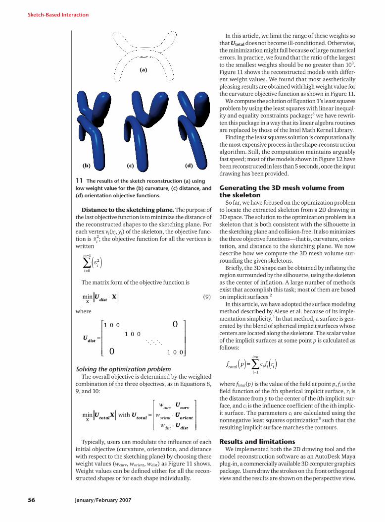
Typically, users can modulate the influence of eachinitial objective (curvature, orientation, and distancewith respect to the sketching plane) by choosing theseweight values (wcurv, worient, wdist) as Figure 11 shows.Weight values can be defined either for all the recon-structed shapes or for each shape individually.

In this article, we limit the range of these weights sothat Utotal does not become ill-conditioned. Otherwise,the minimization might fail because of large numericalerrors. In practice, we found that the ratio of the largestto the smallest weights should be no greater than 103.Figure 11 shows the reconstructed models with differ-ent weight values. We found that most aestheticallypleasing results are obtained with high weight value forthe curvature objective function as shown in Figure 11.

We compute the solution of Equation 1’s least squaresproblem by using the least squares with linear inequal-ity and equality constraints package;8 we have rewrit-ten this package in a way that its linear algebra routinesare replaced by those of the Intel Math Kernel Library.

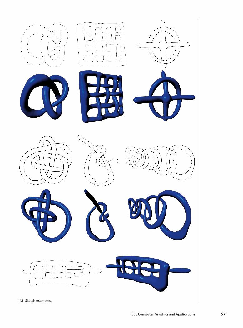
Finding the least squares solution is computationallythe most expensive process in the shape-reconstructionalgorithm. Still, the computation maintains arguablyfast speed; most of the models shown in Figure 12 havebeen reconstructed in less than 5 seconds, once the inputdrawing has been provided.

Generating the 3D mesh volume fromthe skeleton

So far, we have focused on the optimization problemto locate the extracted skeleton from a 2D drawing in3D space. The solution to the optimization problem is askeleton that is both consistent with the silhouette inthe sketching plane and collision-free. It also minimizesthe three objective functions—that is, curvature, orien-tation, and distance to the sketching plane. We nowdescribe how we compute the 3D mesh volume sur-rounding the given skeletons.

Briefly, the 3D shape can be obtained by inflating theregion surrounded by the silhouette, using the skeletonas the center of inflation. A large number of methodsexist that accomplish this task; most of them are basedon implicit surfaces.2

In this article, we have adopted the surface modelingmethod described by Alexe et al. because of its imple-mentation simplicity.3 In that method, a surface is gen-erated by the blend of spherical implicit surfaces whosecenters are located along the skeletons. The scalar valueof the implicit surfaces at some point p is calculated asfollows:

where ftotal(p) is the value of the field at point p, fi is thefield function of the ith spherical implicit surface, ri isthe distance from p to the center of the ith implicit sur-face, and ci is the influence coefficient of the ith implic-it surface. The parameters ci are calculated using thenonnegative least squares optimization8 such that theresulting implicit surface matches the contours.

Results and limitationsWe implemented both the 2D drawing tool and the

model reconstruction software as an AutoDesk Mayaplug-in, a commercially available 3D computer graphicspackage. Users draw the strokes on the front orthogonalview and the results are shown on the perspective view.

f p c f rtotal i i

i

i n

i( ) = ( )=

=

∑1

minX

U U

U

total total

curv

X with =

⋅

⋅

w

wcurv

orientUU

U

orient

distw

dist⋅

⎡

⎣

⎢⎢⎢⎢

⎤

⎦

⎥⎥⎥⎥

Udist

=

⎡

⎣

⎢⎢⎢⎢⎢

⎤

⎦

⎥⎥

1 0 01 0 0

1 0 0

0

0�� ⎥⎥

⎥⎥

minX

Udist

⋅ X

zi

i

m2

0

1

( )=

−

∑

zi2



11 The results of the sketch reconstruction (a) usinglow weight value for the (b) curvature, (c) distance, and(d) orientation objective functions.

(a)

(b) (c) (d)


12 Sketch examples.

We implemented the optimization algorithm with theIntel Math Kernel Library. This numerical package is usedas a library in Maya and includes efficient methods to solvelinear systems involved in the least squares problem.

We have tested our method on different drawingsusing tablet input and evaluated the quality of the recon-structed models. The results are illustrated in Figure 12.Other examples and a demonstration video of our recon-struction algorithm are available at http://vml.kaist.ac.kr/projects.html. All these examples have been calcu-

lated with a high weight value for the curvature objec-tive function. Given an appropriate input drawing, a 3Dmesh is generated in 5 to 10 seconds. Results are com-parable in quality to those obtained from Karpenko,Hughes, and Raskar;2 however, users can now drawobjects that might occlude each other or be self-occlud-ing.

Our algorithm can only reconstruct 3D objects with acircular cross-section. Because of this limitation, mostof the objects created with our tool have a tubular shape.



Previous WorkA drawing of self-occluding objects cannot be processed

in a stroke-based manner, because it typically consists ofmany unclosed curve segments. Thus, we cannot processeach newly drawn curve segment individually, but thereasoning about the drawing can be commenced onlywhen these segments are collectively taken. On the otherhand, there are many technical issues common to ourapproach and previous works on sketching interfaces. Bothrequire analyzing 2D curves provided by the user, andreconstructing corresponding 3D objects from the curves.

Here, we review previous works on sketching interfacesfor 3D graphical modeling, which are clustered accordingto the class of shapes they model. The most commonapproach to 3D modeling with a sketching interface is torequire its user to draw the visible and hidden contours ofthe rectilinear object to be modeled.1 Based on thegeometric correlation hypothesis, such a reconstructiontechnique is particularly suitable for the design of CAD-likegeometric objects. However, the hypothesis theseresearchers use allow modeling of rectilinear objects only.

Some other sketching tools use a purely gesture-basedinterface. For instance, Sketch, proposed by Zeleznik et alidentifies gestures from the input strokes and interpretsthem according to a set of predetermined rules.2 Thoserules define the way the user-supplied gestural symbols aremapped to the creation of primitive objects, or to applyingoperations on existing objects.

Other researchers have presented sketching interfaces forfree-form modeling.3-5 In their systems, users create a shapeby drawing its 2D silhouette; the 3D mesh is generated byinflating the region surrounded by the silhouette, makingwide areas fat and narrow areas thin. The created modelcan then be modified interactively with a set of tools such ascutting, extruding, bending, or drawing on the mesh.

Cohen et al. propose a sketching interface for 3D curvemodeling—the user can model a nonplanar curve bydrawing it from a single viewpoint and its shadow on thefloor plane.6 Other researchers have worked on sketchinginterfaces for modifying existing 3D shapes. In the systemdescribed by Nealen et al., a 3D shape is deformed byfitting its silhouette to a curve given by the user.7

Karpenko and Hughes have published, almostsimultaneously to us, a paper describing a similar system—the modeling of free-form objects with (self-)occlusions.8

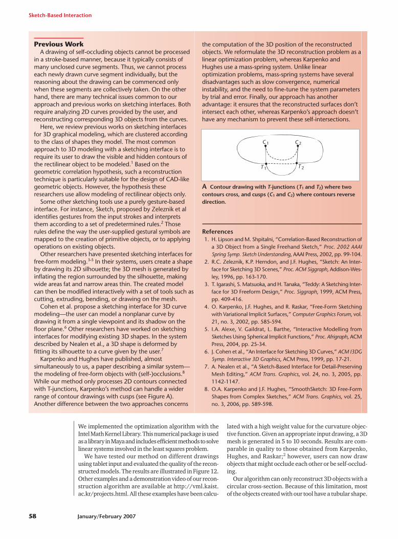
While our method only processes 2D contours connectedwith T-junctions, Karpenko’s method can handle a widerrange of contour drawings with cusps (see Figure A).Another difference between the two approaches concerns

the computation of the 3D position of the reconstructedobjects. We reformulate the 3D reconstruction problem as alinear optimization problem, whereas Karpenko andHughes use a mass-spring system. Unlike linearoptimization problems, mass-spring systems have severaldisadvantages such as slow convergence, numericalinstability, and the need to fine-tune the system parametersby trial and error. Finally, our approach has anotheradvantage: it ensures that the reconstructed surfaces don’tintersect each other, whereas Karpenko’s approach doesn’thave any mechanism to prevent these self-intersections.

A Contour drawing with T-junctions (T1 and T2) where twocontours cross, and cusps (C1 and C2) where contours reversedirection.

References1. H. Lipson and M. Shpitalni, “Correlation-Based Reconstruction of

a 3D Object from a Single Freehand Sketch,” Proc. 2002 AAAISpring Symp. Sketch Understanding, AAAI Press, 2002, pp. 99-104.

2. R.C. Zeleznik, K.P. Herndon, and J.F. Hughes, “Sketch: An Inter-face for Sketching 3D Scenes,” Proc. ACM Siggraph, Addison-Wes-ley, 1996, pp. 163-170.

3. T. Igarashi, S. Matsuoka, and H. Tanaka, “Teddy: A Sketching Inter-face for 3D Freeform Design,” Proc. Siggraph, 1999, ACM Press,pp. 409-416.

4. O. Karpenko, J.F. Hughes, and R. Raskar, “Free-Form Sketchingwith Variational Implicit Surfaces,” Computer Graphics Forum, vol.21, no. 3, 2002, pp. 585-594.

5. I.A. Alexe, V. Gaildrat, L. Barthe, “Interactive Modelling fromSketches Using Spherical Implicit Functions,” Proc. Afrigraph, ACMPress, 2004, pp. 25-34.

6. J. Cohen et al., “An Interface for Sketching 3D Curves,” ACM I3DGSymp. Interactive 3D Graphics, ACM Press, 1999, pp. 17-21.

7. A. Nealen et al., “A Sketch-Based Interface for Detail-PreservingMesh Editing,” ACM Trans. Graphics, vol. 24, no. 3, 2005, pp.1142-1147.

8. O.A. Karpenko and J.F. Hughes, “SmoothSketch: 3D Free-FormShapes from Complex Sketches,” ACM Trans. Graphics, vol. 25,no. 3, 2006, pp. 589-598.

C 1 C 2

T 1 T 2

One way to tackle this limitation would be to extend oursystem to handle interactive shape modification simi-larly to Teddy.1 For instance, users could apply a set ofmodifications such as cut, extrude, or modify the cross-section, on previously created models.

ConclusionWe have presented a method for reconstructing 3D

objects from a 2D drawing, which allows modeling ofobjects with self-occluded parts. The power of ourapproach is best illustrated with the knot exampleshown in Figure 12. To the best of our knowledge, mod-eling of this class of objects is not possible with otherpreviously developed silhouette-based modeling tools.

Another contribution of this work is the formulationof the optimization problem to compute the depth posi-tion of the reconstructed objects. Our mathematicalmodel is simple and its implementation only requirescomputing the elements of the matrices of the objectivefunctions and constraints. In spite of its simplicity, thealgorithm can handle a wide range of cases such as thesketching of groups of flat objects occluding each other,or self-occluding objects that are curved in the z-direc-tion. Our modeler does not place any limitation on thenumber of objects and can handle (self-)occlusions. Inaddition, all input drawings are processed in a uniformmanner. ■

AcknowledgmentsWe thank Sung-Yong Shin, Young-Sang Cho, and

Otfried Cheong (Korea Advanced Institute of Scienceand Technology) for their invaluable advice and use-ful comments. This work was supported by the KoreaResearch Foundation Grant funded by the KoreanGovernment (KRF-2006-531-D00033), and authorCordier was supported by the Graduate School of Cul-ture Technology (Ministry of Culture and Tourism ofKorea).

References1. T. Igarashi, S. Matsuoka, and H. Tanaka, “Teddy: A Sketch-

ing Interface for 3D Freeform Design,” Proc. Siggraph,1999, ACM Press, pp. 409-416.

2. O. Karpenko, J.F. Hughes, and R. Raskar, “Free-FormSketching with Variational Implicit Surfaces,” ComputerGraphics Forum, vol. 21, no. 3, 2002, pp. 585-594.

3. I.A. Alexe, V. Gaildrat, and L. Barthe, “Interactive Model-ling from Sketches Using Spherical Implicit Functions,”Proc. Afrigraph, ACM Press, 2004, pp. 25-34.

4. L.R. Williams, Perceptual Completion of Occluded Surfaces,doctoral dissertation, Dept. Computer Science, Univ. ofMassachusetts at Amherst, 1994.

5. L.R. Williams, “Topological Reconstruction of a SmoothManifold-Solid from Its Occluding Contour,” Int’l J. Com-puter Vision, vol. 23, no. 1, 1997, pp. 93-108.

6. F. Cordier and O. Cheong, “Constrained Delaunay Triangu-lation of Self-Intersecting Polygons,” tech. report, Com-puter Science Dept., KAIST, 2005.

7. W. Wesselink, Variational Modeling of Curves and Surfaces,doctoral dissertation, Dept. Computing Science, Univ. ofTechnology, Eindhoven, 1996.

8. C. Lawson and R. Hanson, Solving Least Squares Problems,Prentice Hall, 1974.

Frederic Cordier is a visiting profes-sor at the Graduate School of CultureTechnology at KAIST. His researchinterests include 3D modeling and tex-turing, human–computer interactionand physics-based simulation. Cordierhas a PhD in computer science from theUniversity of Geneva, Switzerland.

Hyewon Seo is an assistant profes-sor and supervisor of the ComputerGraphics Laboratory in the Depart-ment of Computer Science and Engi-neering at the Chungnam NationalUniversity, Korea. Her research inter-ests include imaging, visual simula-tion, human–computer interaction,

and VR. Seo has graduate degrees in computer science fromthe University of Geneva and KAIST. Contact her [email protected].


The IEEEComputer Society

publishes over 150 conference publications a year.

For a preview of the latest papers in your field, visit

The IEEEComputer Society

publishes over 150 conference publications a year.

For a preview of the latest papers in your field, visit

www.computer.org/publications/

Documents

Free-Form Sketching of Self-