Embed Size (px)
Citation preview

Francisco Porras Bernardez
“EXTRACTION OF USER’S STAYS FROM GPS LOGS: A COMPARISON OF THREE SPATIO-TEMPORAL CLUSTERING APPROACHES”
International Master in Cartography
Wien 16.12.2015

Overview
2
• 1. Introduction • 2. Theory • 3. Method • 4. Implementation • 5. Results • 6. Conclusions
“EXTRACTION OF USER’S STAYS FROM GPS LOGS: A COMPARISON OF THREE SPATIO-TEMPORAL CLUSTERING APPROACHES”

1. Introduction
3
Presence probabilities
Usual places
Normal behaviour
Prediction
Observed behaviour
Visits Transitions
Observation Learning
Visits Transitions
Predicted behaviour
USE CASE
Thesis aim
• 1. Introduction • 2. Theory • 3. Method • 4. Implementation • 5. Results • 6. Conclusions
ICONS from www.flaticon.com

1. Introduction
4
Research identification
Research objectives
(i) Detecting visited places in user’s life in an automated way
(ii) Characterising stays at visited places and transitions between them
Visited place Geographic location in which a user has been located during a minimum period of time (stay).
Stay Physical presence of a user at a geographic location during a period of time.
Transition Change of presence between two different geographic locations in which user has a stay.
Spatio-temporal clustering ICONS from www.flaticon.com

1. Introduction
5
Research questions • Which spatio-temporal clustering approach is the most adequate?
Best algorithm to detect user’s visited places? Differences between tested algorithms? Best values for algorithms parameters?
• Which approach is adequate to characterise stays and transitions?
Relevant information for stays representation? Relevant information for transitions representation?
Research identification
ICONS from www.flaticon.com

2. Theory
6
Clustering algorithms 1. Incremental clustering TBC (Kang et al. 2005) 2. Incremental + density-based clustering TBC (Ye et al. 2009) + DBSCAN (Ester et al. 1996) 3. Density-based clustering DBSCAN (Ester et al. 1996) Quality Evaluation (Salzburg Research 2015) 4 quality measures Confusion matrix
• 1. Introduction • 2. Theory • 3. Method • 4. Implementation • 5. Results • 6. Conclusions

2. Theory
7
Clustering algorithms 1. Incremental clustering (Kang et al. 2005)
• 1. Introduction • 2. Theory • 3. Method • 4. Implementation • 5. Results • 6. Conclusions
Clusters computed incrementally as new location estimates are generated. 2 main parameters: d and t determine number and size of extracted places.
• A stream of coordinates is clustered along time • If stream moves away from current cluster and distance > d new cluster • Smaller clusters, where little time spent, dropped (i1, ... , i5) • If cluster duration: time >= t detected place (A, B)
Third parameter “L” to determine if the user is really moving away from current cluster position If plocs grows beyond L seconds the user is really moving away and starts a new cluster
TBC (Kang et al. 2005)

2. Theory
8
Clustering algorithms 2. Incremental + density-based clustering (Ye et al. 2009)
• 1. Introduction • 2. Theory • 3. Method • 4. Implementation • 5. Results • 6. Conclusions
1st Algorithm (Ye et al. 2009) + 2nd DBSCAN (Ester et al. 1996)
Stay point: a geographic region in which the user stays for a while Two types considered:
Individual maintains stationary at a point for over a time threshold (> t)
(e.g. enters a building)
Individual wanders around within a spatial region (<= d) for over a time threshold (> t)
(e.g. park, square)
• Mean longitude and latitude of GPS points construct a stay point
• Arrival time and leaving time respectively equals timestamp of
first and last GPS point constructing stay point. (P5, P8)

2. Theory
9
Clustering algorithms 2. Incremental + density-based clustering (Ye et al. 2009)
• 1. Introduction • 2. Theory • 3. Method • 4. Implementation • 5. Results • 6. Conclusions
1st Algorithm (Ye et al. 2009) + 2nd DBSCAN (Ester et al. 1996)
Fuzziness of locations Authors perform a second clustering of the initial stay points detected DBSCAN
Final visited place will be the “cluster of the incremental clusters”

2. Theory
10
Clustering algorithms 3. Density-based clustering DBSCAN (Ester et al. 1996)
• 1. Introduction • 2. Theory • 3. Method • 4. Implementation • 5. Results • 6. Conclusions
For each point of a cluster, the cardinality of the neighbourhood of a given
radius (Eps) has to exceed a threshold (MinPts).
i.e. Within an Eps radius, a minimum number of points should be present
Generalizes DBSCAN creating an ordering of the points
- Allows extraction of clusters with arbitrary values for ε (Eps)
- A „maximum Eps“ (ε) to consider is selected as input
- Calculates reachability-distance of every point in dataset
Does not generate a unique clustering, but
Helps choosing optimal Eps
To determine optimum Eps and MinPts auxiliar algorithm DBSCAN
OPTICS (Ankerst et al. 1999)
OPTICS cluster (Ankerst et al. 1999)

2. Theory
11
Clustering algorithms 3. Density-based clustering DBSCAN (Ester et al. 1996)
• 1. Introduction • 2. Theory • 3. Method • 4. Implementation • 5. Results • 6. Conclusions
Reachability plot
- Bar chart that shows each point’s reachability distance in the order the object was processed - Clearly show cluster structure of the data
Eps 6 1 cluster Eps
Eps 4 3 clusters
OPTICS
Choosing optimal Eps
(Ankerst et al. 1999)
Reachability Plot (Ankerst et al. 1999)

Circular buffer around
tagged places
12
Confusion matrix
1. True positive (TP). A tagged (real) place is detected.
2. False negative (FN). A tagged (real) place is not det.
3. False positive (FP). A detection is obtained where
there is no tagged (real) place.
CLASSES
Quality measures
𝑃𝑃𝑃𝑃𝑃𝑃𝑃𝑃𝑃𝑃𝑃𝑃𝑃𝑃𝑃𝑃𝑃𝑃 = 𝑇𝑇𝑃𝑃
𝑇𝑇𝑃𝑃 + 𝐹𝐹𝑃𝑃
𝑅𝑅𝑃𝑃𝑃𝑃𝑅𝑅𝑅𝑅𝑅𝑅 = 𝑇𝑇𝑃𝑃
𝑇𝑇𝑃𝑃 + 𝐹𝐹𝐹𝐹
𝐹𝐹 𝑚𝑚𝑃𝑃𝑅𝑅𝑃𝑃𝑚𝑚𝑃𝑃𝑃𝑃 = 2 ∗ (𝑃𝑃𝑃𝑃𝑃𝑃𝑃𝑃𝑃𝑃𝑃𝑃𝑃𝑃𝑃𝑃𝑃𝑃 ∗ 𝑅𝑅𝑃𝑃𝑃𝑃𝑅𝑅𝑅𝑅𝑅𝑅)𝑃𝑃𝑃𝑃𝑃𝑃𝑃𝑃𝑃𝑃𝑃𝑃𝑃𝑃𝑃𝑃𝑃𝑃 + 𝑅𝑅𝑃𝑃𝑃𝑃𝑅𝑅𝑅𝑅𝑅𝑅
Exactness of the model
Completeness of the model
Effectiveness of retrieval
SPATIAL
1. Spatial accuracy (Qsa)
2. Spatial uniqueness (Qsu)
TEMPORAL
3. Temporal accuracy (Qta)
4. Amount of temporal incorrectness (Qti)
𝑄𝑄𝑡𝑡𝑡𝑡 ≔ 1 −𝐹𝐹𝑡𝑡𝑖𝑖𝑖𝑖𝑖𝑖𝑖𝑖𝑖𝑖𝐷𝐷 =
𝐹𝐹𝑖𝑖𝑖𝑖𝑖𝑖𝑖𝑖𝐷𝐷
Quality Evaluation (Salzburg Research 2015)
2. Theory • 1. Introduction • 2. Theory • 3. Method • 4. Implementation • 5. Results • 6. Conclusions
Detected place = Clusters generated by algorithm
Tagged places = Real locations visited by user (GTD)

3. Method
13
2. Characterisation of stays and transitions between visited places
1. Determination of visited places
Data pre-processing
Spatio-temporal clustering
Thesis innovation
Incremental clustering
Incremental + Density-based clustering
Density-based clustering
• 1. Introduction • 2. Theory • 3. Method • 4. Implementation • 5. Results • 6. Conclusions
TASKS
Ground truth data (GTD). GPS logs:
- Collected by 4 researchers
- 40 days campaign
- 3 sec sampling rate
- Wegeprotokoll with stays and transitions
- Real locations = Tagged Places
Dataset

3. Method
14
• 1. Introduction • 2. Theory • 3. Method • 4. Implementation • 5. Results • 6. Conclusions
1. Determination of visited places 2. Characterization of stays and transitions
2.1. Extraction of stays at visited places - Process for stays extraction
2.2. Extraction of transitions between visited places
- Process for transitions extraction
2.3. Quality Evaluation of the extraction - Confusion matrix - Comparison of different parameter settings
2.4. Characterization of stays and transitions
- User profile and visualizations
1.1. Incremental clustering (Kang et al. 2005) 1.2. Incremental + Density-based clustering (Ye et al. 2009) + DBSCAN (Ester et al. 1996) 1.3. Density-based clustering DBSCAN (Ester et al. 1996) 1.4. Quality Evaluation Implementation (Salzburg Research 2015)
Data pre-processing
Dealing with systematic and random positioning errors
Removal of points with equal timestamp Removal of points with equal geometry Correction of tunnels Removal of spikes
Filtering
Smoothing Kernel based approach

3. Method
15
• 1. Introduction • 2. Theory • 3. Method • 4. Implementation • 5. Results • 6. Conclusions
- Determining visited places in a user’s daily life
- Evaluation of clustering algorithms
- Clusters representing visited places
- Comparison of clustering algorithms performance
- Assessment of the algorithms and selection of the best
GOALS
RESULTS
Quality of the clustering
TARGETS SPATIAL
TEMPORAL
Precision > 66%
Recall > 66%
Times detected > 66%
1. Determination of visited places
ICONS from www.flaticon.com

3. Method
16
• 1. Introduction • 2. Theory • 3. Method • 4. Implementation • 5. Results • 6. Conclusions
- Representing stays at places with characteristic values
- Representing transitions with characteristic values
- Evaluating time extraction performed by spatially best algorithm
- User’s dwell time at significant locations (stays)
- Transitions between significant locations (transitions)
- Evaluation of the stays and transitions extraction
GOALS
RESULTS
2. Characterization of stays and transitions
Quality of the extraction
TARGETS STAYS detection
TRANSITIONS detection
Precision > 66%
Recall > 66%
Precision > 66%
Recall > 66%
ICONS from www.flaticon.com
4. Implementation
17
• 1. Introduction • 2. Theory • 3. Method • 4. Implementation • 5. Results • 6. Conclusions
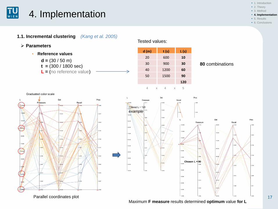
Parameters • Reference values
d = (30 / 50 m) t = (300 / 1800 sec) L = (no reference value)
1.1. Incremental clustering (Kang et al. 2005) Tested values:
d (m) t (s) L (s)
20 600 10
30 900 30
40 1200 60
50 1500 90
120
80 combinations
4 x 4 x 5
Parallel coordinates plot Maximum F measure results determined optimum value for L
example

4. Implementation
18
• 1. Introduction • 2. Theory • 3. Method • 4. Implementation • 5. Results • 6. Conclusions
Parameters
• Tested values
L = 90 sec
Implemented additional Java class for batch processing
1.1. Incremental clustering (Kang et al. 2005)
d (m) t (s) 20 300
26.5 600 30 900 40 1200 53 1500 60 1800 70 2100 80 90
100 200
77 combinations 11 x 7

4. Implementation
19
• 1. Introduction • 2. Theory • 3. Method • 4. Implementation • 5. Results • 6. Conclusions
1.2. Incremental clustering + density-based clustering
- Alternative to DBSCAN - Seamless integration within our process - Almost same performance than DBSCAN - Own solution
1st Algorithm (Ye et al. 2009) + 2nd DBSCAN (Ester et al. 1996) + 2nd ConvexHull
Grouping of points Creation of convex hull Centroid calculation

4. Implementation
20
• 1. Introduction • 2. Theory • 3. Method • 4. Implementation • 5. Results • 6. Conclusions
1.2. Incremental clustering + density-based clustering
1st Algorithm (Ye et al. 2009) + 2nd DBSCAN (Ester et al. 1996) + 2nd ConvexHull
• Tested values
63 combinations
Implemented additional Java class for batch processing
9 x 7
d (m) t (s) 26.5 300 53 600
100 900 200 1200 300 1800 400 2400 500 3000 600 700
g (m)
40
Parameters • Reference values
d = (200 meters) t = (1800 seconds)
g = (40 meters) ConvexHull DBSCAN OPTICS

4. Implementation
21
• 1. Introduction • 2. Theory • 3. Method • 4. Implementation • 5. Results • 6. Conclusions
1.3. Density-based clustering DBSCAN (Ester et al. 1996)
OPTICS (Ankerst et al. 1999)
ELKI Reachability plot for 450.000 points not operative
Alternative visual approach with QGIS
To determine optimal parameters: Eps and MinPts
Java software used for
OPTICS/DBSCAN clustering
ELKI output
DBSCAN clustering with determined Eps
- Represented points with their reachability values
- Represented ground truth places
Chosen reachability determines clusters to be obtained
Visual check of the whole dataset
QGIS
Reachability Plot (Ankerst et al. 1999)

4. Implementation
22
• 1. Introduction • 2. Theory • 3. Method • 4. Implementation • 5. Results • 6. Conclusions
1.3. Density-based clustering DBSCAN (Ester et al. 1996)
• Tested values
77 combinations 11 x 7
MinPts Eps (m) 20 2 30 3 40 6 50 9 60 12 70 15 80 18 90
100 110 120
ELKI
Implemented class for dwell time extraction and batch processing
QGIS
Java

4. Implementation
23
• 1. Introduction • 2. Theory • 3. Method • 4. Implementation • 5. Results • 6. Conclusions
1.4. Quality Evaluation
- Developed at Salzburg Research Mostly implemented within this thesis (Java)
- Applied on 3 spatio-temporal clustering approaches
- Spatial and temporal component of detecting the GTD tagged places
- Measures to evaluate spatial and temporal accuracy of the estimations
- Performance compared in a confusion matrix
Detected places related to tagged places for each test user
Circular buffer around
tagged places
Detected place = Clusters generated by algorithm
Tagged places = Real locations visited by user (GTD)
1. Det. without tagged place
2. Tagged place without det.
3. Multiple detections
4. Mult. tagged places
5. Det. with tagged place
SPATIAL RELATION
TEMPORAL RELATION
∆𝑡𝑡𝑡𝑡,𝑝𝑝 =(𝑡𝑡𝑒𝑒𝑖𝑖𝑡𝑡𝑖𝑖𝑛𝑛,𝑝𝑝 − 𝑡𝑡𝑒𝑒𝑖𝑖𝑡𝑡𝑖𝑖𝑛𝑛,𝑡𝑡) + (𝑡𝑡𝑒𝑒𝑒𝑒𝑡𝑡𝑡𝑡,𝑝𝑝 − 𝑡𝑡𝑒𝑒𝑒𝑒𝑡𝑡𝑡𝑡,𝑡𝑡)
2
Mean time deviation calculated for each tP

4. Implementation
24
• 1. Introduction • 2. Theory • 3. Method • 4. Implementation • 5. Results • 6. Conclusions
2.1. Extraction of stays // 2.2. Extraction of transitions
Stored in each detected place
Duration = texit - tentry
DpID VisitID TimeStart TimeEnd Duration(s) Month Day WD1 0 12/08/2014 16:27 12/08/2014 17:48 4904 8 12 Tue1 1 13/08/2014 16:28 13/08/2014 17:10 2488 8 13 Wed1 2 13/08/2014 17:45 13/08/2014 23:59 22450 8 13 Wed1 2 14/08/2014 00:00 14/08/2014 08:16 29814 8 14 Thu1 3 14/08/2014 16:14 14/08/2014 16:32 1061 8 14 Thu1 4 17/08/2014 18:32 17/08/2014 23:59 19659 8 17 Sun1 4 18/08/2014 00:00 18/08/2014 08:04 29042 8 18 Mon1 5 18/08/2014 16:18 18/08/2014 16:53 2104 8 18 Mon1 6 18/08/2014 17:41 18/08/2014 18:28 2819 8 18 Mon1 7 19/08/2014 16:01 19/08/2014 16:37 2165 8 19 Tue1 8 19/08/2014 18:09 19/08/2014 18:46 2231 8 19 Tue
Stored with associated data
Duration = tentry 2 – texit 1
TrID Orig. Dest. TimeDeparture TimeArrival Distance(m) Duration(s) Sp(km/h) Mon Day WD SameDay1 1 2 12/08/2014 17:48 12/08/2014 17:55 441.0 405 3.920 8 12 Tue TRUE2 2 3 12/08/2014 20:12 13/08/2014 08:17 490.8 43477 0.041 8 12 Tue FALSE3 3 1 13/08/2014 16:01 13/08/2014 16:28 320.4 1623 0.711 8 13 Wed TRUE4 1 1 13/08/2014 17:10 13/08/2014 17:45 0.0 2131 0.000 8 13 Wed TRUE5 1 3 14/08/2014 08:16 14/08/2014 08:23 320.4 423 2.726 8 14 Thu TRUE6 3 1 14/08/2014 16:10 14/08/2014 16:14 320.4 264 4.368 8 14 Thu TRUE7 1 4 14/08/2014 16:32 14/08/2014 18:47 45377.3 8107 20.150 8 14 Thu TRUE8 4 5 14/08/2014 19:28 14/08/2014 19:29 113.6 96 4.260 8 14 Thu TRUE9 5 6 15/08/2014 09:59 15/08/2014 10:03 860.0 192 16.125 8 15 Fri TRUE
10 6 5 15/08/2014 11:59 15/08/2014 12:02 860.0 195 15.877 8 15 Fri TRUE
STAYS
TRANSITIONS

4. Implementation
25
• 1. Introduction • 2. Theory • 3. Method • 4. Implementation • 5. Results • 6. Conclusions
2.3. Quality Evaluation of stays and transitions extraction
Proportion of time extracted
Confusion matrix classes
𝑆𝑆𝑡𝑡𝑒𝑒𝑒𝑒𝑡𝑡 ≔𝑆𝑆𝑡𝑡𝑑𝑑𝑆𝑆𝑡𝑡𝑡𝑡
- True positive (TP) A tagged stay/transition is detected
- False negative (FN) A tagged stay/transition is not detected
- False positive (FP) A stay/transition is obtained when there is no tagged stay/transition
𝑡𝑡�̅�𝑡,𝑑𝑑 =(𝑡𝑡𝑒𝑒𝑖𝑖𝑡𝑡𝑖𝑖𝑛𝑛,𝑑𝑑−𝑡𝑡𝑒𝑒𝑖𝑖𝑡𝑡𝑖𝑖𝑛𝑛,𝑡𝑡) + (𝑡𝑡𝑒𝑒𝑒𝑒𝑡𝑡𝑡𝑡,𝑑𝑑 − 𝑡𝑡𝑒𝑒𝑒𝑒𝑡𝑡𝑡𝑡,𝑡𝑡)
2
𝑃𝑃𝑖𝑖 𝑡𝑡�̅�𝑡,𝑑𝑑 ≤ 900 𝑃𝑃𝑃𝑃𝑃𝑃 → 𝑀𝑀𝑅𝑅𝑡𝑡𝑃𝑃𝑀𝑃𝑃𝑃𝑃
Total time in stays detected
Total time in stays tagged (GTD)
Total time in transitions detected
Total time in transitions tagged (GTD) 𝑇𝑇𝑡𝑡𝑒𝑒𝑒𝑒𝑡𝑡 ≔
𝑇𝑇𝑡𝑡𝑑𝑑𝑇𝑇𝑡𝑡𝑡𝑡

4. Implementation
26
• 1. Introduction • 2. Theory • 3. Method • 4. Implementation • 5. Results • 6. Conclusions
2.4. Characterization of stays and transitions
Number of stays at each tP for each week dayDetected Occurrences GTD Occurrences Proportion of GTD Occurrences detectedTpID Mon Tue Wed Thu Fri Sat Sun SUM TpID Mon Tue Wed Thu Fri Sat Sun SUM TpID Mon Tue Wed Thu Fri Sat Sun PROP
1 3 4 4 2 2 0 0 15 1 8 5 4 6 6 0 0 29 1 0.38 0.80 1.00 0.33 0.33 0.522 0 1 0 0 0 0 0 1 2 1 1 0 0 0 0 0 2 2 0.00 1.00 0.503 4 3 6 8 7 1 4 33 3 11 10 11 12 8 2 7 61 3 0.36 0.30 0.55 0.67 0.88 0.50 0.57 0.544 0 0 0 1 10 14 12 37 4 0 0 0 3 11 16 13 43 4 0.33 0.91 0.88 0.92 0.865 0 0 0 0 1 0 0 1 5 0 0 0 1 1 1 1 4 5 0.00 1.00 0.00 0.00 0.256 0 0 0 1 0 0 0 1 6 0 0 0 1 0 0 0 1 6 1.00 1.007 0 0 0 0 2 1 2 5 7 0 0 0 0 2 2 2 6 7 1.00 0.50 1.00 0.838 0 0 0 0 0 0 1 1 8 0 0 0 0 0 0 1 1 8 1.00 1.009 0 0 0 0 0 0 1 1 9 0 0 0 0 0 0 1 1 9 1.00 1.00
10 0 0 0 1 0 0 0 1 10 0 0 0 1 0 0 0 1 10 1 00 1 00
INDICATORS
1. Number of stays at each tagged place per weekday
1.1. Number of detected occurrences 1.2. Number of GTD occurrences (tagged) 1.3. Proportion of GTD stays detected
2. Duration of the stays at each tagged place per weekday
2.1. Duration of detected stays 2.2. Duration of GTD stays 2.3. Proportion of GTD stays duration detected
• Stays • Transitions 1. Number of transitions between tagged places per weekday
1.1. Number of detected occurrences 1.2. Number of GTD occurrences (tagged) 1.3. Proportion of GTD transitions detected
2. Duration of the transitions between tagged places per weekday
2.1. Duration of detected transitions 2.2. Duration of GTD transitions 2.3. Proportion of GTD transitions duration detected
Stays duration at each tagged place for each weekdayDetected total duration (h) GTD total duration (h) Proportion of GTD total duration detectedTpID Mon Tue Wed Thu Fri Sat Sun SUM TpID Mon Tue Wed Thu Fri Sat Sun SUM TpID Mon Tue Wed Thu Fri Sat Sun PROP
1 23.48 22.02 31.85 13.48 9.10 0.00 0.00 99.93 1 36.73 22.52 31.85 29.77 15.47 0.00 0.00 136.3 1 0.64 0.98 1.00 0.45 0.59 0.732 0.00 2.27 0.00 0.00 0.00 0.00 0.00 2.27 2 0.50 2.27 0.00 0.00 0.00 0.00 0.00 2.77 2 0.00 1.00 0.823 23.48 17.97 40.55 42.20 28.68 11.78 30.35 195.0 3 76.23 65.90 67.03 60.38 36.58 12.28 47.70 366.1 3 0.31 0.27 0.60 0.70 0.78 0.96 0.64 0.534 0.00 0.00 0.00 4.52 37.43 86.80 61.32 190.1 4 0.00 0.00 0.00 5.22 42.98 96.15 61.45 205.8 4 0.87 0.87 0.90 1.00 0.925 0.00 0.00 0.00 0.00 0.93 0.00 0.00 0.93 5 0.00 0.00 0.00 0.10 0.93 3.72 1.60 6.35 5 0.00 1.00 0.00 0.00 0.156 0.00 0.00 0.00 0.65 0.00 0.00 0.00 0.65 6 0.00 0.00 0.00 0.65 0.00 0.00 0.00 0.65 6 1.00 1.007 0.00 0.00 0.00 0.00 5.07 3.13 5.80 14.00 7 0.00 0.00 0.00 0.00 5.07 5.85 5.80 16.72 7 1.00 0.54 1.00 0.848 0.00 0.00 0.00 0.00 0.00 0.00 0.83 0.83 8 0.00 0.00 0.00 0.00 0.00 0.00 0.83 0.83 8 1.00 1.009 0.00 0.00 0.00 0.00 0.00 0.00 1.52 1.52 9 0.00 0.00 0.00 0.00 0.00 0.00 1.52 1.52 9 1.00 1.00
10 0.00 0.00 0.00 1.93 0.00 0.00 0.00 1.93 10 0.00 0.00 0.00 1.93 0.00 0.00 0.00 1.93 10 1.00 1.00
Selection of best clustering algorithm Data mining of algorithm outputs
- Selection according to maximum F measure
- Selection of best parameters settings for the best
algorithm
- Creation of SQLite database
- Design of SQL statements
- Tests with 3 algorithms
- Processing of data for 3D visualizations

5. Results
27
• 1. Introduction • 2. Theory • 3. Method • 4. Implementation • 5. Results • 6. Conclusions
Output tables (example)
- 1. Averaged results from 4 users Algorithms assessment
- 2. Selection of best individual dataset (User1)
- 3. Selection of parameter settings generating highest F measure
- 4. Characterization of stays and transitions from User1
Qsa Distance d (m)Time t (s) 20 26.5 30 40 53 60 70 80 90 100 200
300 0.471 0.499 0.493 0.506 0.507 0.501 0.490 0.486 0.473 0.461 0.313600 0.411 0.438 0.432 0.469 0.475 0.470 0.455 0.450 0.445 0.421 0.325900 0.380 0.393 0.396 0.439 0.443 0.444 0.437 0.429 0.432 0.407 0.313
1200 0.355 0.357 0.360 0.386 0.395 0.399 0.398 0.394 0.397 0.376 0.2861500 0.335 0.328 0.338 0.357 0.366 0.372 0.384 0.378 0.379 0.367 0.3051800 0.306 0.326 0.336 0.351 0.353 0.362 0.381 0.373 0.369 0.353 0.3022100 0.295 0.303 0.317 0.344 0.339 0.358 0.368 0.361 0.367 0.352 0.295
Qsu Distance d (m)Time t (s) 20 26.5 30 40 53 60 70 80 90 100 200
300 0.992 0.996 0.996 1.000 0.996 1.000 0.996 0.996 0.996 0.998 0.994600 0.987 0.995 0.995 1.000 1.000 1.000 0.994 0.994 0.994 0.991 0.995900 1.000 1.000 0.993 1.000 1.000 1.000 0.993 0.993 0.993 0.995 0.993
1200 1.000 1.000 1.000 1.000 1.000 1.000 1.000 1.000 1.000 0.994 0.9911500 1.000 1.000 1.000 1.000 1.000 1.000 1.000 1.000 1.000 0.994 1.0001800 1.000 1.000 1.000 1.000 1.000 1.000 1.000 1.000 1.000 0.993 1.0002100 1.000 1.000 1.000 1.000 1.000 1.000 1.000 1.000 1.000 0.993 1.000
Qta Distance d (m)Time t (s) 20 26.5 30 40 53 60 70 80 90 100 200
300 0.556 0.512 0.522 0.542 0.574 0.590 0.611 0.606 0.577 0.572 0.386600 0.518 0.512 0.506 0.579 0.624 0.648 0.652 0.643 0.614 0.615 0.411900 0.531 0.516 0.503 0.543 0.570 0.612 0.624 0.620 0.589 0.580 0.423
1200 0.529 0.514 0.493 0.566 0.593 0.619 0.629 0.621 0.593 0.586 0.3851500 0.521 0.516 0.523 0.599 0.583 0.622 0.641 0.616 0.594 0.598 0.4191800 0.525 0.564 0.556 0.615 0.570 0.621 0.656 0.633 0.600 0.597 0.4242100 0.526 0.596 0.558 0.616 0.582 0.633 0.659 0.640 0.602 0.603 0.416
Qti Distance d (m)Time t (s) 20 26.5 30 40 53 60 70 80 90 100 200
300 0.452 0.551 0.612 0.664 0.685 0.719 0.788 0.785 0.792 0.817 0.831600 0.492 0.585 0.669 0.667 0.728 0.748 0.784 0.789 0.792 0.799 0.837900 0.549 0.608 0.649 0.705 0.713 0.751 0.777 0.782 0.775 0.808 0.838
1200 0.581 0.640 0.651 0.739 0.739 0.770 0.778 0.791 0.791 0.813 0.8251500 0.570 0.633 0.645 0.737 0.745 0.763 0.774 0.774 0.784 0.798 0.8041800 0.602 0.636 0.651 0.729 0.745 0.759 0.770 0.774 0.803 0.809 0.8052100 0.602 0.655 0.671 0.743 0.776 0.772 0.775 0.773 0.783 0.792 0.834
Recall Distance d (m)Time t (s) 20 26.5 30 40 53 60 70 80 90 100 200
300 0.697 0.737 0.745 0.731 0.728 0.728 0.719 0.720 0.698 0.658 0.503600 0.586 0.617 0.629 0.648 0.649 0.648 0.644 0.654 0.645 0.603 0.488900 0.514 0.522 0.548 0.577 0.581 0.581 0.576 0.597 0.589 0.561 0.453
1200 0.471 0.491 0.499 0.513 0.516 0.518 0.527 0.541 0.531 0.505 0.4271500 0.445 0.459 0.475 0.480 0.484 0.489 0.498 0.507 0.504 0.500 0.4481800 0.414 0.450 0.461 0.462 0.464 0.485 0.489 0.497 0.484 0.473 0.4372100 0.399 0.416 0.435 0.449 0.437 0.467 0.472 0.484 0.463 0.460 0.425
Precision Distance d (m)Time t (s) 20 26.5 30 40 53 60 70 80 90 100 200
300 0.441 0.459 0.470 0.428 0.416 0.413 0.407 0.392 0.372 0.351 0.285600 0.624 0.591 0.610 0.594 0.579 0.585 0.552 0.559 0.556 0.517 0.416900 0.728 0.699 0.722 0.695 0.673 0.661 0.641 0.671 0.664 0.636 0.489
1200 0.750 0.727 0.731 0.736 0.724 0.725 0.698 0.706 0.695 0.673 0.5901500 0.803 0.763 0.783 0.776 0.745 0.762 0.754 0.749 0.736 0.704 0.6571800 0.828 0.785 0.810 0.790 0.775 0.786 0.757 0.777 0.760 0.744 0.6742100 0.846 0.772 0.824 0.802 0.787 0.795 0.764 0.786 0.778 0.757 0.695
Fmeasure Distance d (m)Time t (s) 20 26.5 30 40 53 60 70 80 90 100 200
300 0.539 0.563 0.574 0.538 0.527 0.525 0.518 0.506 0.484 0.457 0.360600 0.600 0.601 0.618 0.619 0.611 0.614 0.594 0.602 0.596 0.554 0.446900 0.600 0.593 0.620 0.628 0.621 0.617 0.604 0.629 0.621 0.593 0.467
1200 0.574 0.582 0.588 0.602 0.600 0.601 0.598 0.609 0.598 0.574 0.4931500 0.568 0.568 0.587 0.591 0.583 0.592 0.596 0.601 0.593 0.580 0.5281800 0.548 0.564 0.583 0.581 0.578 0.596 0.590 0.602 0.588 0.574 0.5242100 0.538 0.534 0.564 0.572 0.557 0.584 0.578 0.593 0.574 0.567 0.520
Detections Distance d (m)Time t (s) 20 26.5 30 40 53 60 70 80 90 100 200
300 115 105 98 101 101 100 99 99 101 102 96600 67 65 62 63 62 61 63 63 62 63 63900 47 47 45 46 47 48 48 47 47 48 50
1200 40 41 40 39 39 39 40 40 41 40 391500 35 36 36 34 35 35 35 36 36 38 371800 31 34 33 33 32 33 34 34 34 34 352100 29 32 31 31 30 32 33 33 32 33 33

5. Results
28
• 1. Introduction • 2. Theory • 3. Method • 4. Implementation • 5. Results • 6. Conclusions
1. Determination of visited places
Algorithms assessment
Best values for each measure and generating parameters
Algorithm KANG YE DBSCAN
Parameters Value Parameters Value Parameters Value
Recall 30 / 300 0.745 100 / 300 0.718 6 / 20 0.770
Precision 20 / 2100 0.846 26.5 / 3000 0.781 2 / 120 0.663
Fmeasure 80 / 900 0.629 100 / 1200 0.575 18 / 110 0.561
Qsa 53 / 300 0.507 53 / 300 0.490 9 / 20 0.493
Qsu Multi 1.000 Multi 1.000 Multi 1.000
Qta 70 / 2100 0.659 26.5 / 3000 0.691 2 / 80 0.852
Qti 200 / 900 0.838 200 / 3000 0.796 15 / 120 0.589
Temporal performance
- Maximum Qta: DBSCAN
- Maximum Qti: Kang
Spatial performance
- Maximum Qsa: Kang
- Maximum Qsu: ALL
Accuracy of times detected
83.8% of times detected are correct
Spatial accuracy of detections (distance/number)
Cases of detections within overlapping areas = 0
• Absolute temporal performance highly dependant on spatial performance
• Without spatial assignment there is no posible temporal assignment
Performance of the clustering Confusion matrix metrics F measure
5. Results
29
• 1. Introduction • 2. Theory • 3. Method • 4. Implementation • 5. Results • 6. Conclusions
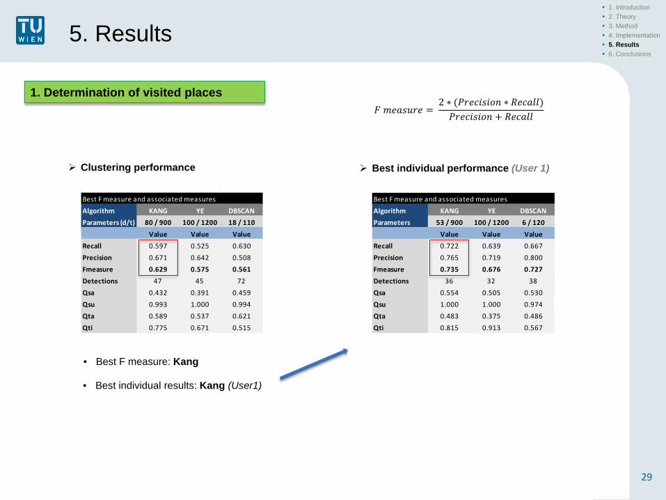
1. Determination of visited places
• Best F measure: Kang
Best F measure and associated measuresAlgorithm KANG YE DBSCANParameters (d/t) 80 / 900 100 / 1200 18 / 110
Value Value ValueRecall 0.597 0.525 0.630Precision 0.671 0.642 0.508Fmeasure 0.629 0.575 0.561Detections 47 45 72Qsa 0.432 0.391 0.459Qsu 0.993 1.000 0.994Qta 0.589 0.537 0.621Qti 0.775 0.671 0.515
Clustering performance
𝐹𝐹 𝑚𝑚𝑃𝑃𝑅𝑅𝑃𝑃𝑚𝑚𝑃𝑃𝑃𝑃 = 2 ∗ (𝑃𝑃𝑃𝑃𝑃𝑃𝑃𝑃𝑃𝑃𝑃𝑃𝑃𝑃𝑃𝑃𝑃𝑃 ∗ 𝑅𝑅𝑃𝑃𝑃𝑃𝑅𝑅𝑅𝑅𝑅𝑅)𝑃𝑃𝑃𝑃𝑃𝑃𝑃𝑃𝑃𝑃𝑃𝑃𝑃𝑃𝑃𝑃𝑃𝑃 + 𝑅𝑅𝑃𝑃𝑃𝑃𝑅𝑅𝑅𝑅𝑅𝑅
• Best individual results: Kang (User1)
Best F measure and associated measuresAlgorithm KANG YE DBSCANParameters 53 / 900 100 / 1200 6 / 120
Value Value ValueRecall 0.722 0.639 0.667Precision 0.765 0.719 0.800Fmeasure 0.735 0.676 0.727Detections 36 32 38Qsa 0.554 0.505 0.530Qsu 1.000 1.000 0.974Qta 0.483 0.375 0.486Qti 0.815 0.913 0.567
Best individual performance (User 1)

5. Results
30
• 1. Introduction • 2. Theory • 3. Method • 4. Implementation • 5. Results • 6. Conclusions
2. Characterization of stays and transitions
Comparison of the extraction (User 1)
Results for the best param. setting for each algorithmAlgorithm KANG YE DBSCANParameters 53 / 900 100 / 1200 6 / 120
Value Value ValueRecall 0.722 0.639 0.667Precision 0.765 0.719 0.800Fmeasure 0.735 0.676 0.727Detections 36 32 38Qsa 0.554 0.505 0.530Qsu 1.000 1.000 0.974Qta 0.483 0.375 0.486Qti 0.815 0.913 0.567 StayT_ext 0.619 0.175 0.468TranT_ext 0.493 0.295 0.373
StRecall 0.600 0.317 0.450StPrecision 0.684 0.471 0.600StFmeas 0.639 0.379 0.514
TrRecall 0.568 0.331 0.374TrPrecision 0.594 0.387 0.452TrFmeas 0.581 0.357 0.409
Stay and Transition time extracted
Stay detection quality
Transition detection quality
Kang
Best performance

5. Results
31
• 1. Introduction • 2. Theory • 3. Method • 4. Implementation • 5. Results • 6. Conclusions
2. Characterization of stays and transitions
Number of stays at each tP for each week dayDetected Occurrences GTD Occurrences Proportion of GTD Occurrences detectedTpID Mon Tue Wed Thu Fri Sat Sun SUM TpID Mon Tue Wed Thu Fri Sat Sun SUM TpID Mon Tue Wed Thu Fri Sat Sun PROP
1 3 4 4 2 2 0 0 15 1 8 5 4 6 6 0 0 29 1 0.38 0.80 1.00 0.33 0.33 0.522 0 1 0 0 0 0 0 1 2 1 1 0 0 0 0 0 2 2 0.00 1.00 0.503 4 3 6 8 7 1 4 33 3 11 10 11 12 8 2 7 61 3 0.36 0.30 0.55 0.67 0.88 0.50 0.57 0.544 0 0 0 1 10 14 12 37 4 0 0 0 3 11 16 13 43 4 0.33 0.91 0.88 0.92 0.865 0 0 0 0 1 0 0 1 5 0 0 0 1 1 1 1 4 5 0.00 1.00 0.00 0.00 0.256 0 0 0 1 0 0 0 1 6 0 0 0 1 0 0 0 1 6 1.00 1.007 0 0 0 0 2 1 2 5 7 0 0 0 0 2 2 2 6 7 1.00 0.50 1.00 0.838 0 0 0 0 0 0 1 1 8 0 0 0 0 0 0 1 1 8 1.00 1.009 0 0 0 0 0 0 1 1 9 0 0 0 0 0 0 1 1 9 1.00 1.00
10 0 0 0 1 0 0 0 1 10 0 0 0 1 0 0 0 1 10 1.00 1.0011 0 1 0 0 0 0 0 1 11 0 1 1 1 0 0 0 3 11 1.00 0.00 0.00 0.3312 0 0 1 0 0 0 0 1 12 0 0 1 0 0 0 0 1 12 1.00 1.0013 0 0 0 0 1 0 0 1 13 0 0 0 0 1 0 0 1 13 1.00 1.0014 0 0 0 0 0 0 0 0 14 0 0 0 0 1 0 0 1 14 0.00 0.0015 0 0 0 0 0 1 0 1 15 0 0 0 0 0 1 0 1 15 1.00 1.0016 0 0 0 0 0 1 0 1 16 0 0 0 0 0 1 0 1 16 1.00 1.0017 0 0 0 0 0 1 0 1 17 0 0 0 0 0 1 0 1 17 1.00 1.0018 0 0 0 0 0 0 1 1 18 0 0 0 0 0 0 1 1 18 1.00 1.0019 0 0 0 0 0 0 1 1 19 0 0 0 0 0 0 1 1 19 1.00 1.0020 1 0 0 0 0 0 0 1 20 1 0 0 0 0 0 0 1 20 1.00 1.0021 0 0 0 0 0 0 0 0 21 1 0 0 0 0 0 0 1 21 0.00 0.0022 0 0 0 0 0 0 0 0 22 1 0 0 0 0 0 0 1 22 0.00 0.0023 0 0 0 0 0 0 0 0 23 1 3 2 2 0 0 0 8 23 0.00 0.00 0.00 0.00 0.0024 0 0 0 0 0 0 0 0 24 0 1 0 0 0 0 0 1 24 0.00 0.0025 0 0 0 0 0 0 0 0 25 0 1 1 1 0 0 0 3 25 0.00 0.00 0.00 0.0026 0 0 0 0 0 0 0 0 26 0 0 1 0 0 0 0 1 26 0.00 0.0027 0 0 0 0 0 0 1 1 27 0 0 0 0 0 0 1 1 27 1.00 1.0028 0 0 0 0 0 0 1 1 28 0 0 0 0 0 0 1 1 28 1.00 1.0029 0 0 0 0 0 1 0 1 29 0 0 0 0 0 1 0 1 29 1.00 1.0030 0 0 0 0 0 0 0 0 30 0 0 0 0 0 1 0 1 30 0.00 0.00
SUM 8 9 11 13 23 20 24 108 SUM 24 22 21 28 30 26 29 180 PROP 0.33 0.41 0.52 0.46 0.77 0.77 0.83 0.60
3 most stayed places
>83% time Home1
Home2
Work
Mondays worst detection
Weekends best detection
Kang (User1) Example of movement behaviour profiling

5. Results
32
• 1. Introduction • 2. Theory • 3. Method • 4. Implementation • 5. Results • 6. Conclusions
2. Characterization of stays and transitions
3 most stayed places
>83% time
Kang (User1)
Stays duration at each tagged place for each weekdayDetected total duration (h) GTD total duration (h) Proportion of GTD total duration detectedTpID Mon Tue Wed Thu Fri Sat Sun SUM TpID Mon Tue Wed Thu Fri Sat Sun SUM TpID Mon Tue Wed Thu Fri Sat Sun PROP
1 23.48 22.02 31.85 13.48 9.10 0.00 0.00 99.93 1 36.73 22.52 31.85 29.77 15.47 0.00 0.00 136.3 1 0.64 0.98 1.00 0.45 0.59 0.732 0.00 2.27 0.00 0.00 0.00 0.00 0.00 2.27 2 0.50 2.27 0.00 0.00 0.00 0.00 0.00 2.77 2 0.00 1.00 0.823 23.48 17.97 40.55 42.20 28.68 11.78 30.35 195.0 3 76.23 65.90 67.03 60.38 36.58 12.28 47.70 366.1 3 0.31 0.27 0.60 0.70 0.78 0.96 0.64 0.534 0.00 0.00 0.00 4.52 37.43 86.80 61.32 190.1 4 0.00 0.00 0.00 5.22 42.98 96.15 61.45 205.8 4 0.87 0.87 0.90 1.00 0.925 0.00 0.00 0.00 0.00 0.93 0.00 0.00 0.93 5 0.00 0.00 0.00 0.10 0.93 3.72 1.60 6.35 5 0.00 1.00 0.00 0.00 0.156 0.00 0.00 0.00 0.65 0.00 0.00 0.00 0.65 6 0.00 0.00 0.00 0.65 0.00 0.00 0.00 0.65 6 1.00 1.007 0.00 0.00 0.00 0.00 5.07 3.13 5.80 14.00 7 0.00 0.00 0.00 0.00 5.07 5.85 5.80 16.72 7 1.00 0.54 1.00 0.848 0.00 0.00 0.00 0.00 0.00 0.00 0.83 0.83 8 0.00 0.00 0.00 0.00 0.00 0.00 0.83 0.83 8 1.00 1.009 0.00 0.00 0.00 0.00 0.00 0.00 1.52 1.52 9 0.00 0.00 0.00 0.00 0.00 0.00 1.52 1.52 9 1.00 1.00
10 0.00 0.00 0.00 1.93 0.00 0.00 0.00 1.93 10 0.00 0.00 0.00 1.93 0.00 0.00 0.00 1.93 10 1.00 1.0011 0.00 8.70 0.00 0.00 0.00 0.00 0.00 8.70 11 0.00 8.70 9.20 9.38 0.00 0.00 0.00 27.28 11 1.00 0.00 0.00 0.3212 0.00 0.00 3.42 0.00 0.00 0.00 0.00 3.42 12 0.00 0.00 3.42 0.00 0.00 0.00 0.00 3.42 12 1.00 1.0013 0.00 0.00 0.00 0.00 1.40 0.00 0.00 1.40 13 0.00 0.00 0.00 0.00 1.40 0.00 0.00 1.40 13 1.00 1.0014 0.00 0.00 0.00 0.00 0.00 0.00 0.00 0.00 14 0.00 0.00 0.00 0.00 0.50 0.00 0.00 0.50 14 0.00 0.0015 0.00 0.00 0.00 0.00 0.00 1.00 0.00 1.00 15 0.00 0.00 0.00 0.00 0.00 1.00 0.00 1.00 15 1.00 1.0016 0.00 0.00 0.00 0.00 0.00 0.70 0.00 0.70 16 0.00 0.00 0.00 0.00 0.00 0.70 0.00 0.70 16 1.00 1.0017 0.00 0.00 0.00 0.00 0.00 2.48 0.00 2.48 17 0.00 0.00 0.00 0.00 0.00 2.48 0.00 2.48 17 1.00 1.0018 0.00 0.00 0.00 0.00 0.00 0.00 0.17 0.17 18 0.00 0.00 0.00 0.00 0.00 0.00 0.17 0.17 18 1.00 1.0019 0.00 0.00 0.00 0.00 0.00 0.00 0.32 0.32 19 0.00 0.00 0.00 0.00 0.00 0.00 0.32 0.32 19 1.00 1.0020 1.27 0.00 0.00 0.00 0.00 0.00 0.00 1.27 20 1.27 0.00 0.00 0.00 0.00 0.00 0.00 1.27 20 1.00 1.0021 0.00 0.00 0.00 0.00 0.00 0.00 0.00 0.00 21 0.80 0.00 0.00 0.00 0.00 0.00 0.00 0.80 21 0.00 0.0022 0.00 0.00 0.00 0.00 0.00 0.00 0.00 0.00 22 0.22 0.00 0.00 0.00 0.00 0.00 0.00 0.22 22 0.00 0.0023 0.00 0.00 0.00 0.00 0.00 0.00 0.00 0.00 23 9.87 14.37 10.88 10.58 0.00 0.00 0.00 45.70 23 0.00 0.00 0.00 0.00 0.0024 0.00 0.00 0.00 0.00 0.00 0.00 0.00 0.00 24 0.00 4.78 0.00 0.00 0.00 0.00 0.00 4.78 24 0.00 0.0025 0.00 0.00 0.00 0.00 0.00 0.00 0.00 0.00 25 0.00 4.28 8.32 7.55 0.00 0.00 0.00 20.15 25 0.00 0.00 0.00 0.0026 0.00 0.00 0.00 0.00 0.00 0.00 0.00 0.00 26 0.00 0.00 3.13 0.00 0.00 0.00 0.00 3.13 26 0.00 0.0027 0.00 0.00 0.00 0.00 0.00 0.00 1.83 1.83 27 0.00 0.00 0.00 0.00 0.00 0.00 1.83 1.83 27 1.00 1.0028 0.00 0.00 0.00 0.00 0.00 0.00 1.22 1.22 28 0.00 0.00 0.00 0.00 0.00 0.00 1.22 1.22 28 1.00 1.0029 0.00 0.00 0.00 0.00 0.00 0.73 0.00 0.73 29 0.00 0.00 0.00 0.00 0.00 0.73 0.00 0.73 29 1.00 1.0030 0.00 0.00 0.00 0.00 0.00 0.00 0.00 0.00 30 0.00 0.00 0.00 0.00 0.00 0.35 0.00 0.35 30 0.00 0.00
SUM 48.2 50.9 75.8 62.8 82.6 106.6 103.3 530.4 SUM 125.6 122.8 133.8 125.6 102.9 123.3 122.4 856.5 PROP 0.38 0.41 0.57 0.50 0.80 0.87 0.84 0.62
Home1
Home2
Work
Mondays worst detection
Weekends best detection
Example of movement behaviour profiling

5. Results
33
• 1. Introduction • 2. Theory • 3. Method • 4. Implementation • 5. Results • 6. Conclusions
2. Characterization of stays and transitions
Kang (User1) Transitions between tagged places for each weekdayDetected total duration (h) GTD total duration (h) Proportion of GTD total duration detectedTran Mon Tue Wed Thu Fri Sat Sun SUM Tran Mon Tue Wed Thu Fri Sat Sun SUM Tran Mon Tue Wed Thu Fri Sat Sun PROP01-01 0.00 0.15 0.00 0.00 0.00 0.00 0.00 0.15 01-01 0.25 0.15 0.00 0.28 0.18 0.00 0.00 0.87 01-01 0.00 1.00 0.00 0.00 0.1701-02 0.00 0.00 0.00 0.00 0.00 0.00 0.00 0.00 01-02 0.27 1.92 0.00 0.00 0.00 0.00 0.00 2.18 01-02 0.00 0.00 0.0001-03 0.38 0.35 0.80 0.30 0.50 0.00 0.00 2.33 01-03 0.50 0.35 0.92 0.60 0.50 0.00 0.00 2.87 01-03 0.77 1.00 0.87 0.50 1.00 0.8101-31 0.00 0.00 0.00 0.00 0.00 0.00 0.00 0.00 01-31 0.00 0.00 0.00 0.00 0.10 0.00 0.00 0.10 01-31 0.00 0.0002-01 0.00 0.00 0.00 0.00 0.00 0.00 0.00 0.00 02-01 2.60 0.00 0.00 0.00 0.00 0.00 0.00 2.60 02-01 0.00 0.0002-03 0.00 0.00 0.00 0.00 0.00 0.00 0.00 0.00 02-03 0.00 0.15 0.00 0.00 0.00 0.00 0.00 0.15 02-03 0.00 0.0003-01 0.42 0.12 0.13 0.38 0.52 0.00 0.00 1.57 03-01 0.72 0.35 0.47 0.53 0.52 0.00 0.00 2.58 03-01 0.58 0.33 0.29 0.72 1.00 0.6103-03 0.82 1.45 0.33 0.30 0.00 0.00 0.00 2.90 03-03 0.82 1.45 0.33 0.30 0.00 0.72 0.00 3.62 03-03 1.00 1.00 1.00 1.00 0.00 0.8003-04 0.00 0.00 0.00 0.00 2.82 0.00 0.00 2.82 03-04 0.00 0.00 0.00 1.25 4.95 0.00 0.00 6.20 03-04 0.00 0.57 0.4503-10 0.00 0.00 0.00 0.00 0.00 0.00 0.00 0.00 03-10 0.00 0.00 0.00 0.62 0.00 0.00 0.00 0.62 03-10 0.00 0.0003-11 0.00 0.00 0.00 0.00 0.00 0.00 0.00 0.00 03-11 0.00 0.32 0.12 0.28 0.00 0.00 0.00 0.72 03-11 0.00 0.00 0.00 0.0003-12 0.00 0.00 0.00 0.00 0.00 0.00 0.00 0.00 03-12 0.00 0.00 0.55 0.00 0.00 0.00 0.00 0.55 03-12 0.00 0.0003-13 0.00 0.00 0.00 0.00 1.53 0.00 0.00 1.53 03-13 0.00 0.00 0.00 0.00 1.53 0.00 0.00 1.53 03-13 1.00 1.0003-19 0.57 0.00 0.00 0.00 0.00 0.00 0.00 0.57 03-19 0.57 0.00 0.00 0.00 0.00 0.00 0.00 0.57 03-19 1.00 1.0003-26 0.00 0.00 0.00 0.00 0.00 0.00 1.70 1.70 03-26 0.00 0.00 0.00 0.00 0.00 0.00 1.70 1.70 03-26 1.00 1.0004-03 0.00 0.00 0.00 0.00 0.00 0.00 2.37 2.37 04-03 0.00 0.00 0.00 0.00 0.00 0.00 5.88 5.88 04-03 0.40 0.4004-04 0.00 0.00 0.00 0.00 2.70 4.13 1.87 8.70 04-04 0.00 0.00 0.00 0.00 2.70 4.28 1.87 8.85 04-04 1.00 0.96 1.00 0.9804-05 0.00 0.00 0.00 0.00 0.55 0.10 0.10 0.75 04-05 0.00 0.00 0.00 0.10 0.55 0.10 0.10 0.85 04-05 0.00 1.00 1.00 1.00 0.8804-06 0.00 0.00 0.00 0.00 0.00 0.00 0.00 0.00 04-06 0.00 0.00 0.00 0.05 0.00 0.00 0.00 0.05 04-06 0.00 0.0004-07 0.00 0.00 0.00 0.00 0.20 0.12 0.12 0.43 04-07 0.00 0.00 0.00 0.00 0.20 0.12 0.12 0.43 04-07 1.00 1.00 1.00 1.0004-08 0.00 0.00 0.00 0.00 0.00 0.00 0.12 0.12 04-08 0.00 0.00 0.00 0.00 0.00 0.00 0.12 0.12 04-08 1.00 1.0004-09 0.00 0.00 0.00 0.00 0.00 0.00 0.83 0.83 04-09 0.00 0.00 0.00 0.00 0.00 0.00 0.83 0.83 04-09 1.00 1.0004-14 0.00 0.00 0.00 0.00 0.00 0.67 0.00 0.67 04-14 0.00 0.00 0.00 0.00 0.00 0.67 0.00 0.67 04-14 1.00 1.0004-16 0.00 0.00 0.00 0.00 0.00 0.13 0.00 0.13 04-16 0.00 0.00 0.00 0.00 0.00 0.13 0.00 0.13 04-16 1.00 1.0004-17 0.00 0.00 0.00 0.00 0.00 0.00 0.00 0.00 04-17 0.00 0.00 0.00 0.00 0.00 0.00 3.87 3.87 04-17 0.00 0.0004-28 0.00 0.00 0.00 0.00 0.00 0.27 0.00 0.27 04-28 0.00 0.00 0.00 0.00 0.00 0.27 0.00 0.27 04-28 1.00 1.0005-04 0.00 0.00 0.00 0.00 0.10 0.00 0.00 0.10 05-04 0.00 0.00 0.00 0.10 0.10 0.12 0.17 0.48 05-04 0.00 1.00 0.00 0.00 0.2106-04 0.00 0.00 0.00 0.03 0.00 0.00 0.00 0.03 06-04 0.00 0.00 0.00 0.03 0.00 0.00 0.00 0.03 06-04 1.00 1.0007-04 0.00 0.00 0.00 0.00 0.17 0.10 0.17 0.43 07-04 0.00 0.00 0.00 0.00 0.17 0.13 0.17 0.47 07-04 1.00 0.75 1.00 0.9308-04 0.00 0.00 0.00 0.00 0.00 0.00 2.15 2.15 08-04 0.00 0.00 0.00 0.00 0.00 0.00 2.15 2.15 08-04 1.00 1.0009-04 0.00 0.00 0.00 0.00 0.00 0.00 0.62 0.62 09-04 0.00 0.00 0.00 0.00 0.00 0.00 0.62 0.62 09-04 1.00 1.0010-03 0.00 0.00 0.00 0.27 0.00 0.00 0.00 0.27 10-03 0.00 0.00 0.00 0.27 0.00 0.00 0.00 0.27 10-03 1.00 1.0011-03 0.00 0.43 0.00 0.00 0.00 0.00 0.00 0.43 11-03 0.00 0.43 0.00 0.27 0.00 0.00 0.00 0.70 11-03 1.00 0.00 0.6212-03 0.00 0.00 0.00 0.00 0.00 0.00 0.00 0.00 12-03 0.00 0.00 0.15 0.00 0.00 0.00 0.00 0.15 12-03 0.00 0.0013-04 0.00 0.00 0.00 0.00 0.15 0.00 0.00 0.15 13-04 0.00 0.00 0.00 0.00 0.15 0.00 0.00 0.15 13-04 1.00 1.0014-15 0.00 0.00 0.00 0.00 0.00 0.00 0.00 0.00 14-15 0.00 0.00 0.00 0.00 0.00 0.88 0.00 0.88 14-15 0.00 0.0015-04 0.00 0.00 0.00 0.00 0.00 1.55 0.00 1.55 15-04 0.00 0.00 0.00 0.00 0.00 1.55 0.00 1.55 15-04 1.00 1.0016-04 0.00 0.00 0.00 0.00 0.00 0.17 0.00 0.17 16-04 0.00 0.00 0.00 0.00 0.00 0.17 0.00 0.17 16-04 1.00 1.0017-18 0.00 0.00 0.00 0.00 0.00 0.00 0.00 0.00 17-18 0.00 0.00 0.00 0.00 0.00 0.00 1.48 1.48 17-18 0.00 0.0018-04 0.00 0.00 0.00 0.00 0.00 0.00 1.33 1.33 18-04 0.00 0.00 0.00 0.00 0.00 0.00 1.33 1.33 18-04 1.00 1.0019-20 0.00 0.00 0.00 0.00 0.00 0.00 0.00 0.00 19-20 0.93 0.00 0.00 0.00 0.00 0.00 0.00 0.93 19-20 0.00 0.0020-21 0.00 0.00 0.00 0.00 0.00 0.00 0.00 0.00 20-21 3.10 0.00 0.00 0.00 0.00 0.00 0.00 3.10 20-21 0.00 0.0021-22 0.00 0.00 0.00 0.00 0.00 0.00 0.00 0.00 21-22 0.42 0.00 0.00 0.00 0.00 0.00 0.00 0.42 21-22 0.00 0.0022-23 0.00 0.00 0.00 0.00 0.00 0.00 0.00 0.00 22-23 0.00 0.10 0.00 0.00 0.00 0.00 0.00 0.10 22-23 0.00 0.0022-24 0.00 0.00 0.00 0.00 0.00 0.00 0.00 0.00 22-24 0.00 0.13 0.17 0.20 0.00 0.00 0.00 0.50 22-24 0.00 0.00 0.00 0.0023-22 0.00 0.00 0.00 0.00 0.00 0.00 0.00 0.00 23-22 0.00 0.15 0.00 0.00 0.00 0.00 0.00 0.15 23-22 0.00 0.0024-22 0.00 0.00 0.00 0.00 0.00 0.00 0.00 0.00 24-22 0.00 0.18 0.00 0.17 0.00 0.00 0.00 0.35 24-22 0.00 0.00 0.0024-25 0.00 0.00 0.00 0.00 0.00 0.00 0.00 0.00 24-25 0.00 0.00 0.67 0.00 0.00 0.00 0.00 0.67 24-25 0.00 0.0025-22 0.00 0.00 0.00 0.00 0.00 0.00 0.00 0.00 25-22 0.00 0.00 0.83 0.00 0.00 0.00 0.00 0.83 25-22 0.00 0.0026-27 0.00 0.00 0.00 0.00 0.00 0.00 0.12 0.12 26-27 0.00 0.00 0.00 0.00 0.00 0.00 0.12 0.12 26-27 1.00 1.0027-03 0.00 0.00 0.00 0.00 0.00 0.00 1.05 1.05 27-03 0.00 0.00 0.00 0.00 0.00 0.00 1.05 1.05 27-03 1.00 1.0028-29 0.00 0.00 0.00 0.00 0.00 0.00 0.00 0.00 28-29 0.00 0.00 0.00 0.00 0.00 0.55 0.00 0.55 28-29 0.00 0.0029-04 0.00 0.00 0.00 0.00 0.00 0.00 0.00 0.00 29-04 0.00 0.00 0.00 0.00 0.00 0.05 0.00 0.05 29-04 0.00 0.0031-01 0.00 0.00 0.00 0.00 0.00 0.00 0.00 0.00 31-01 0.00 0.00 0.00 0.00 5.42 0.00 0.00 5.42 31-01 0.00 0.00SUM 2.18 2.50 1.27 1.28 9.23 7.23 12.53 36.23 SUM 10.17 5.68 4.20 5.05 17.07 9.73 21.57 73.47 PROP 0.21 0.44 0.3 0.25 0.54 0.74 0.58 0.49
Wednesdays worst detection
Weekends best detection
Work Home1
Home1 Work Home1 Home1
Home2 Home2 Home2 Home1
Home1 Home2
Fri.: Long time spent moving
Home1 Home2
Sun.: Long time spent moving
Home2 Home1
Sat.: Long time spent moving
around Home2
Trips by plane

5. Results
34
• 1. Introduction • 2. Theory • 3. Method • 4. Implementation • 5. Results • 6. Conclusions
2. Characterization of stays and transitions - Tagged stays and detected stays
- Green cylinder at detected places
Tagged place
Detected place
Detected stays Tagged stays
Kang (User1)
Visualization of movement behaviour
6. Conclusions
35
• 1. Introduction • 2. Theory • 3. Method • 4. Implementation • 5. Results • 6. Conclusions
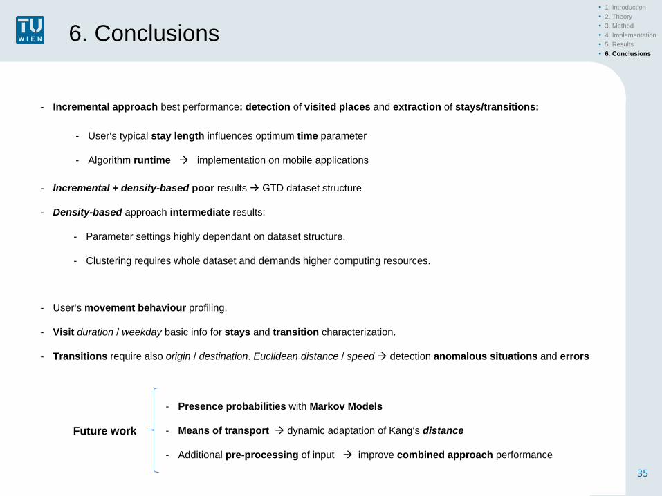
- Incremental approach best performance: detection of visited places and extraction of stays/transitions:
- User‘s typical stay length influences optimum time parameter
- Algorithm runtime implementation on mobile applications
- Incremental + density-based poor results GTD dataset structure
- Density-based approach intermediate results:
- Parameter settings highly dependant on dataset structure.
- Clustering requires whole dataset and demands higher computing resources.
- User‘s movement behaviour profiling.
- Visit duration / weekday basic info for stays and transition characterization.
- Transitions require also origin / destination. Euclidean distance / speed detection anomalous situations and errors
- Presence probabilities with Markov Models
- Means of transport dynamic adaptation of Kang‘s distance
- Additional pre-processing of input improve combined approach performance
Future work

THANK YOU VERY MUCH FOR YOUR ATTENTION !
Muchas gracias por su atención !
And, thank you very much:

References
37
• Ankerst, M. et al., 1999. Optics: Ordering points to identify the clustering structure. In ACM Sigmod Record. pp. 49–60. Available at: http://dl.acm.org/citation.cfm?id=304187.
• Ester, M. et al., 1996. A Density-Based Algorithm for Discovering Clusters in Large Spatial Databases with Noise. In Second International Conference on Knowledge Discovery and Data Mining. pp. 226–231. Available at: http://citeseerx.ist.psu.edu/viewdoc/summary?doi=10.1.1.20.2930.
• Kang, J.H. et al., 2005. Extracting places from traces of locations. ACM SIGMOBILE Mobile Computing and Communications Review, 9(3), p.58. Available at: http://portal.acm.org/citation.cfm?doid=1024733.1024748 [Accessed August 13, 2014].
• Montoliu, R., Blom, J. & Gatica-Perez, D., 2013. Discovering places of interest in everyday life from smartphone data. Multimedia Tools and Applications, 62, pp.179–207.
• Shekhar, S., Zhang, P. & Huang, Y., 2003. Trends in Spatial Data Mining. Science, 7, pp.357–379. Available at: http://citeseerx.ist.psu.edu/viewdoc/download?doi=10.1.1.77.1454&rep=rep1&type=pdf.
• Ye, Y. et al., 2009. Mining individual life pattern based on location history. Proceedings - IEEE International Conference on Mobile Data Management, pp.1–10.
• Salzburg Research Forschungsgesellschaft mbH, 2015. (Internal reports).