Collect. Math.DOI 10.1007/s13348-013-0091-6

Frames for decomposition spaces generatedby a single function

Morten Nielsen

Received: 28 January 2013 / Accepted: 13 July 2013© Universitat de Barcelona 2013

Abstract In this paper we present a construction of frames generated by a single band-limited function for decomposition smoothness spaces on R

d of modulation and Triebel–Lizorkin type. A perturbation argument is then used to construct compactly supported framegenerators.

Keywords Decomposition space · Smoothness space · Banach frame · Single generator

Mathematics Subject Classification (2000) 42C15 · 42C40

1 Introduction

Sparse representations of signals relative to a fixed time-frequency system play an importantrole in approximation theory, numerical analysis, and for practical applications. The mostprominent example being sparse wavelet representation of signals, which is an approach withmany applications to modern technology. However, wavelets are not a universal fix for everysparse representation problem, and depending on the “nature” of the signals to be analysed,it might be more advantageous to choose a representation system with significantly differenttime-frequency properties such as Gabor systems or perhaps curvelet-type frames.

Two aspects of sparse representations that will be in focus in this paper are the flexibility toadapt the representation system to the signal and the fact that a discrete sparse representationof a function (signal) is often linked to some notion of smoothness of the function. The factthat sparseness in general is linked to smoothness is an observation that that goes all the

Supported by the Danish Council for Independent Research. Natural Sciences, Grant 12-124675,“Mathematical and Statistical Analysis of Spatial Data”.

M. Nielsen (B)Department of Mathematical Sciences, Aalborg University,Fredrik Bajersvej 7G, 9220 Aalborg East, Denmarke-mail: mnielsen@math.aau.dk

123

M. Nielsen

way back to the study of Fourier series for C1-functions, but the link is perhaps even moretransparant in the modern theory of function spaces based on Littlewood–Paley theory.

The path we follow here is to study the link between discrete sparse representations andsmoothness within the framework of so-called decomposition smoothness spaces. We alsoinsist that smoothness should be linked to sparseness using a simple representation systemgenerated by a single function similar to case for wavelet and Gabor systems.

Decomposition spaces were introduced by Feichtinger and Gröbner [10] and Feichtinger[7], and are based on structured coverings R

d considered either as the direct (time-variable)space or the frequency space. One major advantage of this set up is the flexibility. Very generaldecompositions of the frequency space fit in this framework yielding flexibility that alsoallows an anisotropic setup to be considered without much added complexity. For example,classical Triebel–Lizorkin and Besov spaces fit nicely into the decomposition space modeland they correspond to dyadic coverings of the frequency space, see [25]. Modulation spacesalso fit into the model and they correspond to uniform coverings of the frequency place, see[8]. In recent years, many authors have found the decomposition approach useful, see e.g.[5,6,12,15,16,21,22].

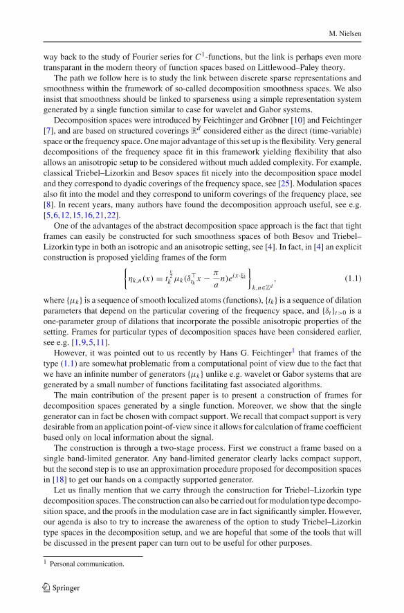
One of the advantages of the abstract decomposition space approach is the fact that tightframes can easily be constructed for such smoothness spaces of both Besov and Triebel–Lizorkin type in both an isotropic and an anisotropic setting, see [4]. In fact, in [4] an explicitconstruction is proposed yielding frames of the form{

ηk,n(x) = tν2

k μk(δ�tk x − π

an)eix ·ξk

}k,n∈Zd

, (1.1)

where {μk} is a sequence of smooth localized atoms (functions), {tk} is a sequence of dilationparameters that depend on the particular covering of the frequency space, and {δt }t>0 is aone-parameter group of dilations that incorporate the possible anisotropic properties of thesetting. Frames for particular types of decomposition spaces have been considered earlier,see e.g. [1,9,5,11].

However, it was pointed out to us recently by Hans G. Feichtinger1 that frames of thetype (1.1) are somewhat problematic from a computational point of view due to the fact thatwe have an infinite number of generators {μk} unlike e.g. wavelet or Gabor systems that aregenerated by a small number of functions facilitating fast associated algorithms.

The main contribution of the present paper is to present a construction of frames fordecomposition spaces generated by a single function. Moreover, we show that the singlegenerator can in fact be chosen with compact support. We recall that compact support is verydesirable from an application point-of-view since it allows for calculation of frame coefficientbased only on local information about the signal.

The construction is through a two-stage process. First we construct a frame based on asingle band-limited generator. Any band-limited generator clearly lacks compact support,but the second step is to use an approximation procedure proposed for decomposition spacesin [18] to get our hands on a compactly supported generator.

Let us finally mention that we carry through the construction for Triebel–Lizorkin typedecomposition spaces. The construction can also be carried out for modulation type decompo-sition space, and the proofs in the modulation case are in fact significantly simpler. However,our agenda is also to try to increase the awareness of the option to study Triebel–Lizorkintype spaces in the decomposition setup, and we are hopeful that some of the tools that willbe discussed in the present paper can turn out to be useful for other purposes.

1 Personal communication.

123

Frames for decomposition spaces generated by a single function

2 Decomposition type smoothness spaces on Rd

We begin by introducing some machinery needed for the definition of decomposition spaces.First we study a homogeneous structure on R

d that will be used to generated general coveringsof the the frequency space, and moreover, it also offers the flexibility to incorporate anisotropyinto the general construction.

2.1 A homoneneous structure on Rd

Here we define homogeneous type spaces on Rd which will be used later to construct a suitable

covering of the frequency space. These spaces are created with a quasi-norm induced by aone-parameter group of dilations. Let | · | denote the Euclidean norm on R

d induced by theinner product 〈·, ·〉. We assume that A is a real d × d matrix with eigenvalues having positivereal parts. For t > 0 define the group of dilations δt : R

d → Rd by δt := exp(A ln t) and

let ν := trace(A). The matrix A will be kept fixed throughout the paper. Some well-knownproperties of δt are (see [24]),

• δts = δtδs .• δ1 = I d (identity on R

d ).• δtξ is jointly continuous in t and ξ , and δtξ → 0 as t → 0+.• |δt | := det(δt ) = tν .

According to [24, Proposition 1.7] there exists a strictly positive symmetric matrix P suchthat for all ξ ∈ R

d ,

[δtξ ]P := 〈Pδtξ, δtξ 〉12

is a strictly increasing function of t. This helps us to introduce a quasi-norm | · |A associatedwith A.

Definition 2.1 We define the function | · |A : Rd → R+ by |0|A := 0 and for ξ ∈ R

d\{0}by letting |ξ |A be the unique solution t to the equation [δ1/tξ ]P = 1.

It can be shown that:

• There exists a constant CA > 0 such that

|ξ + ζ |A ≤ CA(|ξ |A + |ζ |A), ξ, ζ ∈ Rd .

• |δtξ |A = t |ξ |A.• There exists constants C1,C2, α1, α2 > 0 such that

C1 min(|ξ |α1A , |ξ |α2

A ) ≤ |ξ | ≤ C2 max(|ξ |α1A , |ξ |α2

A ), ξ ∈ Rd . (2.1)

Example 2.2 For A = diag(β1, β2, . . . , βd), βi > 0, we have δt = diag(tβ1 , tβ2 , . . . , tβd ),and one can verify that

|ξ |A �d∑

j=1

|ξ j |1β j , ξ ∈ R

d .

We need an extension of the quantity 〈ξ 〉 := (1 + |ξ |2)1/2 to the non-isotropic setting. Let Abe the (d + 1)× (d + 1) matrix given by[

1 00 A

],

123

M. Nielsen

and define Dt = exp( A ln t). For (ζ, ξ) ∈ R × Rd , we have Dt (ζ, ξ) = (tζ, δtξ). We let

|(ζ, ξ)| A be the unique solution t to [[D1/t (ζ, ξ)]]P = 1, where [[(ζ, ξ)]]P := (ζ 2+[ξ ]2P )

1/2.Notice that |(1, 0)| A = 1 and |(0, ξ)| A = |ξ |A. For ξ ∈ R

d , we define the bracket 〈ξ 〉A :=|(1, ξ)| A.

Finally, we define the balls BA(ξ, r) := {ζ ∈ Rd : |ξ − ζ |A < r}. It can be verified that

|BA(ξ, r)| = rνωAd , where ωA

d := |BA(0, 1)|, so (Rd , | · |A, dξ) is a space of homogeneoustype with homogeneous dimension ν.

The transpose of A with respect to 〈·, ·〉, B := A�, will be useful for generating coveringsof the direct space R

d . Since the eigenvalues of B have positive real parts we can repeat theabove construction for the group δ�t := exp(B ln t), t > 0. We let | · |B denote the quasi-norm induced by δ�t , and let 〈·〉B denote the bracket corresponding to the group δ�t . The ballsassociated with | · |B are denoted BB(ξ, r). Furthermore, we have that (2.1) holds with thesame constants α1 and α2 for | · |B . Notice that if gm(x) := mνg(δ�m x), g ∈ L2(R

d), thengm(ξ) = g(δ 1

mξ). We use the convention that δt acts on the frequency space while δ�t acts

on the direct space.The following adaption of the Fefferman–Stein maximal inequality to the quasi-norm | · |B

will be essential for showing the boundedness of almost diagonal matrices. For 0 < r < ∞,the anisotropic maximal function of Hardy–Littlewood type is defined by

M Br u(x) := sup

t>0

⎛⎜⎝ 1

ωBd · tν

∫BB (x,t)

|u(y)|r dy

⎞⎟⎠

1r

, u ∈ Lr,loc(Rd), (2.2)

whereωBd := |BB(0, 1)|. We also need the vector-valued Fefferman–Stein maximal inequal-

ity. For 0 < p, q ≤ ∞, and a sequence f = { f j } j∈N of L p(Rd) functions, we define the

norm

‖ f ‖L p(�q ) :=

∥∥∥∥∥∥∥

⎛⎝∑

j∈N

| f j |q⎞⎠

1/q∥∥∥∥∥∥∥

L p(Rd )

.

With this notation, there exists C > 0 so that the following vector-valued maximal inequalityholds for r < q ≤ ∞ and r < p < ∞ (see [23, Chapters I&II]),∥∥{M B

r fk}k∥∥

L p(�q )≤ C

∥∥{ fk}k∥∥

L p(�q ). (2.3)

If q = ∞, then the inner lq -norm is replaced by the l∞-norm.We introduce the following Peetre-type maximal function. Let u(x) be a continuous func-

tion on Rd . We define

u∗(a, R; x) := supy∈Rd

〈y〉−aB |u(x − δ−�

R y)|, a, R > 0, x ∈ Rd ,

where we use the notation δ−�R := (δ−1

R )�.It is clear that u∗(a, R; x) is finite whenever u is bounded. However, for band-limited

functions we can obtain a much more interesting estimate of u∗(a, R; x) in terms of theanisotropic maximal function. It can be shown (see [4, Proposition 3.3]) that for r, R > 0,there exist a constant C := C(R, r) such that for any function u(x) on R

d with supp(u) ⊂BA(0, R), we have

u∗(ν/r, R; x) ≤ C M Br u(x), ∀x ∈ R

d . (2.4)

123

Frames for decomposition spaces generated by a single function

This result can be considered in the vector-valued setting. Let � = {�n} be a sequence ofcompact subsets of R

d , and let

L�p (�q) := {{ fn}n∈N ∈ L p(�q) | supp( fn) ⊆ �n, ∀n}.Then the following proposition holds, see [4, Corollary 3.4].

Proposition 2.3 Suppose 0 < p < ∞ and 0 < q ≤ ∞, and let � = {TkC }k∈N be asequence of compact subsets of R

d generated by a family {Tk = δtk · +ξk}k∈N of invertibleaffine transformations on R

d , with C a fixed compact subset of Rd . If 0 < r < min(p, q),

then there exists a constant K such that∥∥∥∥{ supz∈Rd

〈δ�tk z〉−ν/rB | fk(· − z)|}

∥∥∥∥L p(�q )

≤ K‖{ fk}‖L p(�q ), (2.5)

for all f ∈ L�p (�q), where f = { fk}k∈N.

Finally we consider a result on vector-valued Fourier multipliers that will be needed tostudy stability of smoothness spaces in the following section. For s ∈ R we let

‖ f ‖Hs2

:=(∫

|F−1 f (x)|2〈x〉2sB dx

)1/2

(2.6)

denote the (anisotropic) Sobolev space norm. Notice that for f ∈ Hs2 , 0 < ε0 ≤ t < ∞, and

ξk ∈ Rd , we have ‖ f (δt ·+ξk)‖Hs

2≤ Cts−ν/2‖ f ‖Hs

2< ∞ with C depending only on ε0. For

f ∈ S (Rd) and � ∈ S ′(Rd), we define �(D) f := F−1(� f ). The following Theorem isproved in [4].

Theorem 2.4 Suppose 0 < p < ∞ and 0 < q ≤ ∞. Let � = {TkC }k∈N be a sequenceof compact subsets of R

d generated by a family {Tk = δtk · +ξk}k∈N of invertible affinetransformations, with C a fixed compact subset of R

d . Assume {ψ j } j∈N is a sequence offunctions satisfying ψ j ∈ Hs

2 for some s > ν2 + ν

min(p,q) . Then there exists a constantC < ∞ such that

‖{ψk(D) fk}‖L p(�q ) ≤ C supj

‖ψ j (Tj ·)‖Hs2

· ‖{ fk}‖L p(�q )

for all { fk}k∈N ∈ L�p (�q).

2.2 Decomposition spaces and adapted frames

We now introduce so-called admissible coverings and show how to generate them. Thesecoverings are then used to construct a suitable resolution of unity and next define Triebel–Lizorkin type smoothness spaces and associated modulation spaces. Finally, we construct aframe which will be used in the following sections to generate compactly supported frameexpansions.

Definition 2.5 A set Q := {Qk}k∈Zd of measurable subsets Qk ⊂ Rd is called an admissible

covering if Rd = ∪k∈Zd Qk and there exists n0 < ∞ such that #{ j ∈ Z

d : Qk∩Q j �= ∅} ≤ n0

for all k ∈ Zd .

To generate an admissible covering we will use a suitable collection of | · |A-balls, where theradius of a given ball is a so-called moderate function of its center.

123

M. Nielsen

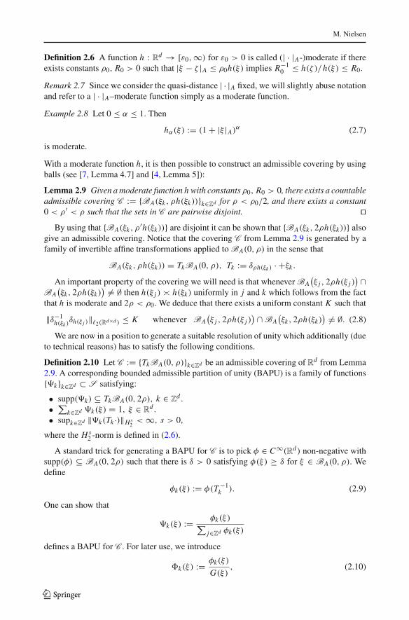
Definition 2.6 A function h : Rd → [ε0,∞) for ε0 > 0 is called (| · |A-)moderate if there

exists constants ρ0, R0 > 0 such that |ξ − ζ |A ≤ ρ0h(ξ) implies R−10 ≤ h(ζ )/h(ξ) ≤ R0.

Remark 2.7 Since we consider the quasi-distance | · |A fixed, we will slightly abuse notationand refer to a | · |A–moderate function simply as a moderate function.

Example 2.8 Let 0 ≤ α ≤ 1. Then

hα(ξ) := (1 + |ξ |A)α (2.7)

is moderate.

With a moderate function h, it is then possible to construct an admissible covering by usingballs (see [7, Lemma 4.7] and [4, Lemma 5]):

Lemma 2.9 Given a moderate function h with constants ρ0, R0 > 0, there exists a countableadmissible covering C := {BA(ξk, ρh(ξk))}k∈Zd for ρ < ρ0/2, and there exists a constant0 < ρ′ < ρ such that the sets in C are pairwise disjoint. ��

By using that {BA(ξk, ρ′h(ξk))} are disjoint it can be shown that {BA(ξk, 2ρh(ξk))} also

give an admissible covering. Notice that the covering C from Lemma 2.9 is generated by afamily of invertible affine transformations applied to BA(0, ρ) in the sense that

BA(ξk, ρh(ξk)) = TkBA(0, ρ), Tk := δρh(ξk ) · +ξk .

An important property of the covering we will need is that whenever BA(ξ j , 2ρh(ξ j )

)∩BA(ξk, 2ρh(ξk)

) �= ∅ then h(ξ j ) � h(ξk) uniformly in j and k which follows from the factthat h is moderate and 2ρ < ρ0. We deduce that there exists a uniform constant K such that

‖δ−1h(ξk )

δh(ξ j )‖�2(Rd×d ) ≤ K whenever BA(ξ j , 2ρh(ξ j )

) ∩ BA(ξk, 2ρh(ξk)

) �= ∅. (2.8)

We are now in a position to generate a suitable resolution of unity which additionally (dueto technical reasons) has to satisfy the following conditions.

Definition 2.10 Let C := {TkBA(0, ρ)}k∈Zd be an admissible covering of Rd from Lemma

2.9. A corresponding bounded admissible partition of unity (BAPU) is a family of functions{�k}k∈Zd ⊂ S satisfying:

• supp(�k) ⊆ TkBA(0, 2ρ), k ∈ Zd .

• ∑k∈Zd �k(ξ) = 1, ξ ∈ Rd .

• supk∈Zd ‖�k(Tk ·)‖Hs2< ∞, s > 0,

where the Hs2 -norm is defined in (2.6).

A standard trick for generating a BAPU for C is to pick φ ∈ C∞(Rd) non-negative withsupp(φ) ⊆ BA(0, 2ρ) such that there is δ > 0 satisfying φ(ξ) ≥ δ for ξ ∈ BA(0, ρ). Wedefine

φk(ξ) := φ(T −1k ). (2.9)

One can show that

�k(ξ) := φk(ξ)∑j∈Zd φk(ξ)

defines a BAPU for C . For later use, we introduce

�k(ξ) := φk(ξ)

G(ξ), (2.10)

123

Frames for decomposition spaces generated by a single function

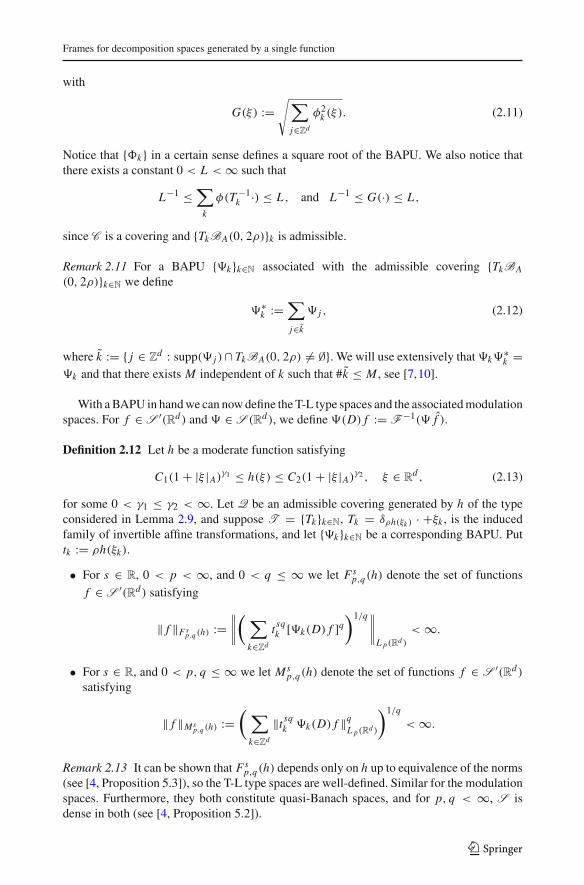
with

G(ξ) :=√∑

j∈Zd

φ2k (ξ). (2.11)

Notice that {�k} in a certain sense defines a square root of the BAPU. We also notice thatthere exists a constant 0 < L < ∞ such that

L−1 ≤∑

k

φ(T −1k ·) ≤ L , and L−1 ≤ G(·) ≤ L ,

since C is a covering and {TkBA(0, 2ρ)}k is admissible.

Remark 2.11 For a BAPU {�k}k∈N associated with the admissible covering {TkBA

(0, 2ρ)}k∈N we define

�∗k :=

∑j∈k

� j , (2.12)

where k := { j ∈ Zd : supp(� j )∩ TkBA(0, 2ρ) �= ∅}. We will use extensively that�k�

∗k =

�k and that there exists M independent of k such that #k ≤ M , see [7,10].

With a BAPU in hand we can now define the T-L type spaces and the associated modulationspaces. For f ∈ S ′(Rd) and � ∈ S (Rd), we define �(D) f := F−1(� f ).

Definition 2.12 Let h be a moderate function satisfying

C1(1 + |ξ |A)γ1 ≤ h(ξ) ≤ C2(1 + |ξ |A)

γ2 , ξ ∈ Rd , (2.13)

for some 0 < γ1 ≤ γ2 < ∞. Let Q be an admissible covering generated by h of the typeconsidered in Lemma 2.9, and suppose T = {Tk}k∈N, Tk = δρh(ξk ) · +ξk , is the inducedfamily of invertible affine transformations, and let {�k}k∈N be a corresponding BAPU. Puttk := ρh(ξk).

• For s ∈ R, 0 < p < ∞, and 0 < q ≤ ∞ we let Fsp,q(h) denote the set of functions

f ∈ S ′(Rd) satisfying

‖ f ‖Fsp,q (h) :=

∥∥∥∥( ∑

k∈Zd

t sqk [�k(D) f ]q

)1/q∥∥∥∥L p(Rd )

< ∞.

• For s ∈ R, and 0 < p, q ≤ ∞ we let Msp,q(h) denote the set of functions f ∈ S ′(Rd)

satisfying

‖ f ‖Msp,q (h) :=

( ∑k∈Zd

‖t sqk �k(D) f ‖q

L p(Rd )

)1/q

< ∞.

Remark 2.13 It can be shown that Fsp,q(h) depends only on h up to equivalence of the norms

(see [4, Proposition 5.3]), so the T-L type spaces are well-defined. Similar for the modulationspaces. Furthermore, they both constitute quasi-Banach spaces, and for p, q < ∞, S isdense in both (see [4, Proposition 5.2]).

123

M. Nielsen

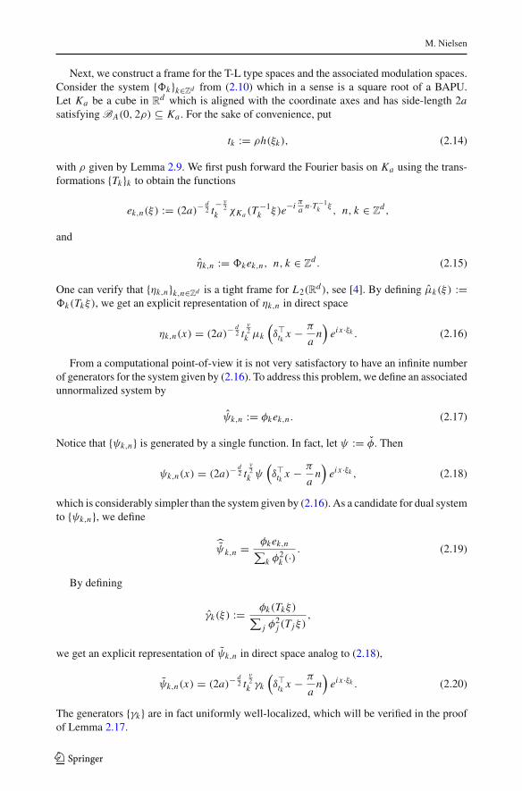
Next, we construct a frame for the T-L type spaces and the associated modulation spaces.Consider the system {�k}k∈Zd from (2.10) which in a sense is a square root of a BAPU.Let Ka be a cube in R

d which is aligned with the coordinate axes and has side-length 2asatisfying BA(0, 2ρ) ⊆ Ka . For the sake of convenience, put

tk := ρh(ξk), (2.14)

with ρ given by Lemma 2.9. We first push forward the Fourier basis on Ka using the trans-formations {Tk}k to obtain the functions

ek,n(ξ) := (2a)−d2 t

− ν2

k χKa (T−1

k ξ)e−i πa n·T −1k ξ

, n, k ∈ Zd ,

and

ηk,n := �kek,n, n, k ∈ Zd . (2.15)

One can verify that {ηk,n}k,n∈Zd is a tight frame for L2(Rd), see [4]. By defining μk(ξ) :=

�k(Tkξ), we get an explicit representation of ηk,n in direct space

ηk,n(x) = (2a)−d2 t

ν2

k μk

(δ�tk x − π

an)

eix ·ξk . (2.16)

From a computational point-of-view it is not very satisfactory to have an infinite numberof generators for the system given by (2.16). To address this problem, we define an associatedunnormalized system by

ψk,n := φkek,n . (2.17)

Notice that {ψk,n} is generated by a single function. In fact, let ψ := φ. Then

ψk,n(x) = (2a)−d2 t

ν2

k ψ(δ�tk x − π

an)

eix ·ξk , (2.18)

which is considerably simpler than the system given by (2.16). As a candidate for dual systemto {ψk,n}, we define

ψk,n = φkek,n∑

k φ2k (·)

. (2.19)

By defining

γk(ξ) := φk(Tkξ)∑j φ

2j (Tjξ)

,

we get an explicit representation of ψk,n in direct space analog to (2.18),

ψk,n(x) = (2a)−d2 t

ν2

k γk

(δ�tk x − π

an)

eix ·ξk . (2.20)

The generators {γk} are in fact uniformly well-localized, which will be verified in the proofof Lemma 2.17.

123

Frames for decomposition spaces generated by a single function

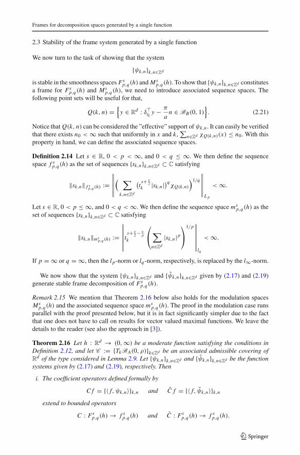
2.3 Stability of the frame system generated by a single function

We now turn to the task of showing that the system

{ψk,n}k,n∈Zd

is stable in the smoothness spaces Fsp,q(h) and Ms

p,q(h). To show that {ψk,n}k,n∈Zd constitutesa frame for Fs

p,q(h) and Msp,q(h), we need to introduce associated sequence spaces. The

following point sets will be useful for that,

Q(k, n) ={

y ∈ Rd : δ�tk y − π

an ∈ BB(0, 1)

}. (2.21)

Notice that Q(k, n) can be considered the ”effective” support ofψk,n . It can easily be verifiedthat there exists n0 < ∞ such that uniformly in x and k,

∑n∈Zd χQ(k,n)(x) ≤ n0. With this

property in hand, we can define the associated sequence spaces.

Definition 2.14 Let s ∈ R, 0 < p < ∞, and 0 < q ≤ ∞. We then define the sequencespace f s

p,q(h) as the set of sequences {sk,n}k,n∈Zd ⊂ C satisfying

‖sk,n‖ f sp,q (h) :=

∥∥∥∥∥∥( ∑

k,n∈Zd

(ts+ ν

2k |sk,n |)qχQ(k,n)

)1/q

∥∥∥∥∥∥L p

< ∞.

Let s ∈ R, 0 < p ≤ ∞, and 0 < q < ∞. We then define the sequence space msp,q(h) as the

set of sequences {sk,n}k,n∈Zd ⊂ C satisfying

‖sk,n‖msp,q (h) :=

∥∥∥∥∥∥∥ts+ ν

2 − νp

k

⎛⎝∑

n∈Zd

|sk,n |p

⎞⎠

1/p∥∥∥∥∥∥∥

lq

< ∞.

If p = ∞ or q = ∞, then the l p-norm or lq -norm, respectively, is replaced by the l∞-norm.

We now show that the system {ψk,n}k,n∈Zd and {ψk,n}k,n∈Zd given by (2.17) and (2.19)generate stable frame decomposition of Fs

p,q(h).

Remark 2.15 We mention that Theorem 2.16 below also holds for the modulation spacesMs

p,q(h) and the associated sequence space msp,q(h). The proof in the modulation case runs

parallel with the proof presented below, but it is in fact significantly simpler due to the factthat one does not have to call on results for vector valued maximal functions. We leave thedetails to the reader (see also the approach in [3]).

Theorem 2.16 Let h : Rd → (0,∞) be a moderate function satisfying the conditions in

Definition 2.12, and let C := {TkBA(0, ρ)}k∈Zd be an associated admissible covering ofR

d of the type considered in Lemma 2.9. Let {ψk,n}k,n∈Zd and {ψk,n}k,n∈Zd be the functionsystems given by (2.17) and (2.19), respectively. Then

i. The coefficient operators defined formally by

C f = {〈 f, ψk,n〉}k,n and C f = {〈 f, ψk,n〉}k,n

extend to bounded operators

C : Fsp,q(h) → f s

p,q(h) and C : Fsp,q(h) → f s

p,q(h).

123

M. Nielsen

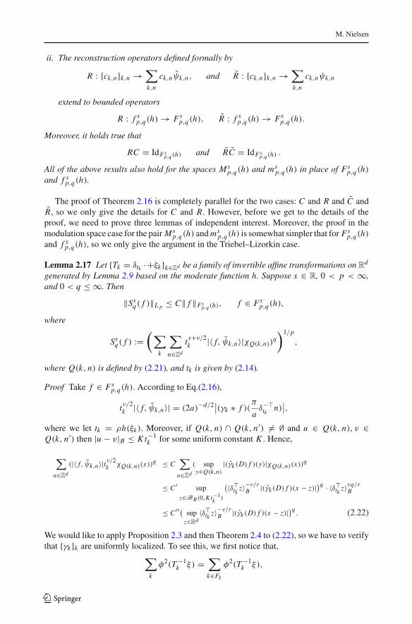
ii. The reconstruction operators defined formally by

R : {ck,n}k,n →∑k,n

ck,nψk,n, and R : {ck,n}k,n →∑k,n

ck,nψk,n

extend to bounded operators

R : f sp,q(h) → Fs

p,q(h), R : f sp,q(h) → Fs

p,q(h).

Moreover, it holds true that

RC = IdFsp,q (h) and RC = IdFs

p,q (h) .

All of the above results also hold for the spaces Msp,q(h) and ms

p,q(h) in place of Fsp,q(h)

and f sp,q(h).

The proof of Theorem 2.16 is completely parallel for the two cases: C and R and C andR, so we only give the details for C and R. However, before we get to the details of theproof, we need to prove three lemmas of independent interest. Moreover, the proof in themodulation space case for the pair Ms

p,q(h) and msp,q(h) is somewhat simpler that for Fs

p,q(h)and f s

p,q(h), so we only give the argument in the Triebel–Lizorkin case.

Lemma 2.17 Let {Tk = δtk ·+ξk}k∈Zd be a family of invertible affine transformations on Rd

generated by Lemma 2.9 based on the moderate function h. Suppose s ∈ R, 0 < p < ∞,and 0 < q ≤ ∞. Then

‖Ssq( f )‖L p ≤ C‖ f ‖Fs

p,q (h), f ∈ Fsp,q(h),

where

Ssq( f ) :=

(∑k

∑n∈Zd

t s+ν/2k |〈 f, ψk,n〉|χQ(k,n))

q)1/p

,

where Q(k, n) is defined by (2.21), and tk is given by (2.14).

Proof Take f ∈ Fsp,q(h). According to Eq.(2.16),

tν/2k |〈 f, ψk,n〉| = (2a)−d/2∣∣(γk ∗ f )(

π

aδ−�

tk n)∣∣,

where we let tk = ρh(ξk). Moreover, if Q(k, n) ∩ Q(k, n′) �= ∅ and u ∈ Q(k, n), v ∈Q(k, n′) then |u − v|B ≤ K t−1

k for some uniform constant K . Hence,

∑n∈Zd

(|〈 f, ψk,n〉|tν/2k χQ(k,n)(x))q ≤ C

∑n∈Zd

( supy∈Q(k,n)

|(γk (D) f )(y)|χQ(k,n)(x))q

≤ C ′ supz∈BB (0,K t−1

k )

(〈δ�tk z〉−ν/rB |(γk (D) f )(x − z)|)q · 〈δ�tk z〉νq/r

B

≤ C ′′( supz∈Rd

〈δ�tk z〉−ν/rB |(γk (D) f )(x − z)|)q . (2.22)

We would like to apply Proposition 2.3 and then Theorem 2.4 to (2.22), so we have to verifythat {γk}k are uniformly localized. To see this, we first notice that,∑

k

φ2(T −1k ξ) =

∑k∈Fξ

φ2(T −1k ξ),

123

Frames for decomposition spaces generated by a single function

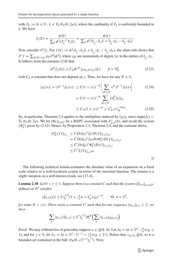
with Fξ := {k ∈ N : ξ ∈ TkBA(0, 2ρ)}, where the cardinality if Fξ is uniformly bounded inξ . We have

γ j (ξ) = φ(ξ)∑k φ

2(T −1k Tjξ)

= φ(ξ)∑k φ

2(δt−1kδt j ξ + δt−1

kξ j − δt−1

kξk).

Now consider ∂αγ j . For f (ξ) := φ2(δt−1kδt j ξ + δt−1

kξ j − δt−1

kξk), the chain rule shows that

∂η f =∑β:|β|=|η| pβ∂β [φ2], where pβ are monomials of degree |η| in the entries of δt−1kδt j .

It follows from the estimate (2.8) that

|∂β γ j (ξ)| ≤ CβK |β|χBA(0,2ρ)(ξ), β ∈ Nd0 , (2.23)

with Cβ a constant that does not depend on j . Thus, we have for any N ∈ N,

|γk(x)| = |F−1γk(x)| ≤ C(1 + |x |)−N∣∣∣∣∑

|β|≤N

xβF−1γk(x)

∣∣∣∣ (2.24)

≤ C(1 + |x |)−N∑

|β|≤N

‖∂βξ γk‖L1

≤ CN (1 + |x |)−N ≤ C ′N 〈x〉−Nα1

B . (2.25)

So, in particular, Theorem 2.4 applies to the multipliers induced by {γk}k since supp(γk) ⊂TkBA(0, 2ρ). We let {�k}k∈Zd be a BAPU associated with Fs

p,q(h), and recall the system{�∗

k } given by (2.12). Hence, by Proposition 2.3, Theorem 2.4, and the estimate above,

‖Ssq( f )‖L p ≤ C‖h(ξk)

s γk(D) f ‖L p(�q )

= C‖h(ξk)s γk(D)�

∗k (D) f ‖L p(�q )

≤ C ′‖h(ξk)s�∗

k (D) f ‖L p(�q )

≤ C ′′‖ f ‖Fsp,q (h).

��

The following technical lemma estimates the absolute value of an expansion on a fixedscale relative to a well-localized system in terms of the maximal function. The lemma is aslight variation on a well-known result, see [17,4].

Lemma 2.18 Let 0 < r ≤ 1. Suppose there is a constant C such that the system {ψk,n}k,n∈Zd

defined on Rd satisfies

|ψk,n(x)| ≤ Ctν/2k (1 + |πa n + δ�tk x |B)−N , ∀k, n ∈ Z

d ,

for some N > ν/r . There exists a constant C ′ such that for any sequence {sk,n}k,n ⊂ C, wehave ∑

n

|sk,n ||ψk,n | ≤ C ′tν/2k M Br

(∑n

|sk,n |χQ(k,n)

).

Proof We may without loss of generality suppose x ∈ Q(k, 0). Let A0 = {n ∈ Zd : |πa n|B ≤

1}, and for j ∈ N, let A j = {n ∈ Zd : 2 j−1 < |πa n|B ≤ 2 j }. Notice that ∪n∈A j Q(k, n) is a

bounded set contained in the ball BB(0, c2 j+1t−1k ). Now,

123

M. Nielsen

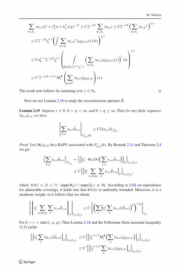
∑n∈A j

|sk,n |(1 + |πa n + δ�tk x |B)−N ≤ C2− j N

∑n∈A j

|sk,n | ≤ C2− j N(∑

n∈A j

|sk,n |r)1/r

≤ C2− j N tν/rk

(∫ ∑n∈A j

|sk,n |rχQ(k,n)(y) dy

)1/r

≤ Cn1−r0 2− j N tν/r

k

⎛⎜⎜⎝

∫

BB (0,c2 j+1t−1k )

(∑n∈A j

|sk,n |χQ(k,n)(y))r

dy

⎞⎟⎟⎠

1/r

≤ C ′2− j (N−ν/r)M Br

⎛⎝∑

n∈Zd

|sk,n |χQ(k,n)

⎞⎠ (x).

The result now follows by summing over j ∈ N0. ��

Next we use Lemma 2.18 to study the reconstruction operator R.

Lemma 2.19 Suppose s ∈ R, 0 < p < ∞, and 0 < q ≤ ∞. Then for any finite sequence{sk,n}k,n, we have

∥∥∥∥∥∥∑k,n

sk,nψk,n

∥∥∥∥∥∥Fs

p,q (h)

≤ C‖{sk,n}‖ f sp,q.

Proof Let {�k}k∈N be a BAPU associated with Fsp,q(h). By Remark 2.11 and Theorem 2.4

we get

∥∥∥∑k,n

sk,nψk,n

∥∥∥Fs

p,q

=∥∥∥{t s

k ·�k(D)(∑�,n

s�,nψ�,n)}

k

∥∥∥L p(�q )

≤ C∥∥∥{t s

k

∑�∈N (k)

∑n

s�,nψ�,n}

k

∥∥∥L p(�q )

,

where N (k) = {� ∈ N : supp(�k) ∩ supp(ψ�) �= ∅}. According to [10] on equivalencefor admissible coverings, it holds true that #N (k) is uniformly bounded. Moreover, h is amoderate weight, so it follows that we obtain

∥∥∥∥∥∥

⎧⎨⎩t s

k

∑�∈N (k)

∑n

s�,nψ�,n

⎫⎬⎭

k

∥∥∥∥∥∥L p(�q )

≤ C

∥∥∥∥∥(∑

�

(t s�

∑n

|s�,n ||ψ�,n |)q)1/q

∥∥∥∥∥L p

.

Fix 0 < r < min(1, p, q). Then Lemma 2.18 and the Fefferman–Stein maximal inequality(2.3) yields

∥∥∥{t sk

∑n

|sk,n ||ψk,n |}

k

∥∥∥L p(�q )

≤ C∥∥∥{t s+ν/2

k M Br

(∑n

|sk,n |χQ(k,n)

)}k

∥∥∥L p(�q )

≤ C ′∥∥∥{t s+ν/2

k

∑n

|sk,n |χQ(k,n)

}k

∥∥∥L p(�q )

.

123

Frames for decomposition spaces generated by a single function

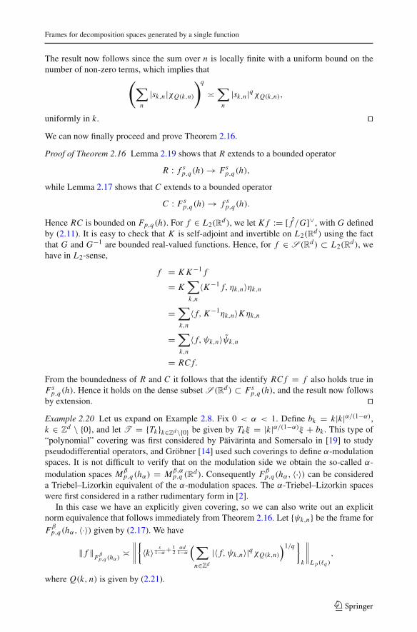
The result now follows since the sum over n is locally finite with a uniform bound on thenumber of non-zero terms, which implies that(∑

n

|sk,n |χQ(k,n)

)q

�∑

n

|sk,n |qχQ(k,n),

uniformly in k. ��We can now finally proceed and prove Theorem 2.16.

Proof of Theorem 2.16 Lemma 2.19 shows that R extends to a bounded operator

R : f sp,q(h) → Fs

p,q(h),

while Lemma 2.17 shows that C extends to a bounded operator

C : Fsp,q(h) → f s

p,q(h).

Hence RC is bounded on Fp,q(h). For f ∈ L2(Rd), we let K f := [ f /G]∨, with G defined

by (2.11). It is easy to check that K is self-adjoint and invertible on L2(Rd) using the fact

that G and G−1 are bounded real-valued functions. Hence, for f ∈ S (Rd) ⊂ L2(Rd), we

have in L2-sense,

f = K K −1 f

= K∑k,n

〈K −1 f, ηk,n〉ηk,n

=∑k,n

〈 f, K −1ηk,n〉Kηk,n

=∑k,n

〈 f, ψk,n〉ψk,n

= RC f.

From the boundedness of R and C it follows that the identify RC f = f also holds true inFs

p,q(h). Hence it holds on the dense subset S (Rd) ⊂ Fsp,q(h), and the result now follows

by extension. ��Example 2.20 Let us expand on Example 2.8. Fix 0 < α < 1. Define bk = k|k|α/(1−α),k ∈ Z

d \ {0}, and let T = {Tk}k∈Zd\{0} be given by Tkξ = |k|α/(1−α)ξ + bk . This type of“polynomial” covering was first considered by Päivärinta and Somersalo in [19] to studypseudodifferential operators, and Gröbner [14] used such coverings to define α-modulationspaces. It is not difficult to verify that on the modulation side we obtain the so-called α-modulation spaces Mβ

p,q(hα) = Mβ,αp,q (R

d). Consequently Fβp,q(hα, 〈·〉) can be considereda Triebel–Lizorkin equivalent of the α-modulation spaces. The α-Triebel–Lizorkin spaceswere first considered in a rather rudimentary form in [2].

In this case we have an explicitly given covering, so we can also write out an explicitnorm equivalence that follows immediately from Theorem 2.16. Let {ψk,n} be the frame forFβp,q(hα, 〈·〉) given by (2.17). We have

‖ f ‖Fβp,q (hα)

�∥∥∥∥{〈k〉 s

1−α+ 12αd

1−α(∑

n∈Zd

|〈 f, ψk,n〉|qχQ(k,n)

)1/q}

k

∥∥∥∥L p(�q )

,

where Q(k, n) is given by (2.21).

123

M. Nielsen

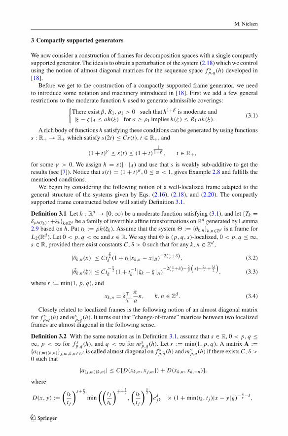
3 Compactly supported generators

We now consider a construction of frames for decomposition spaces with a single compactlysupported generator. The idea is to obtain a perturbation of the system (2.18) which we controlusing the notion of almost diagonal matrices for the sequence space f s

p,q(h) developed in[18].

Before we get to the construction of a compactly supported frame generator, we needto introduce some notation and machinery introduced in [18]. First we add a few generalrestrictions to the moderate function h used to generate admissible coverings:{

There existβ, R1, ρ1 > 0 such that h1+β is moderate and|ξ − ζ |A ≤ ah(ξ) for a ≥ ρ1 implies h(ζ ) ≤ R1 ah(ξ).

(3.1)

A rich body of functions h satisfying these conditions can be generated by using functionss : R+ → R+ which satisfy s(2t) ≤ Cs(t), t ∈ R+, and

(1 + t)γ ≤ s(t) ≤ (1 + t)1

1+β , t ∈ R+,

for some γ > 0. We assign h = s(| · |A) and use that s is weakly sub-additive to get theresults (see [7]). Notice that s(t) = (1 + t)α, 0 ≤ α < 1, gives Example 2.8 and fulfills thementioned conditions.

We begin by considering the following notion of a well-localized frame adapted to thegeneral structure of the systems given by Eqs. (2.16), (2.18), and (2.20). The compactlysupported frame constructed below will satisfy Definition 3.1.

Definition 3.1 Let h : Rd → [0,∞) be a moderate function satisfying (3.1), and let {Tk =

δρh(ξk ) ·+ξk}k∈Zd be a family of invertible affine transformations on Rd generated by Lemma

2.9 based on h. Put tk := ρh(ξk). Assume that the system � := {θk,n}k,n∈Zd is a frame forL2(R

d). Let 0 < p, q < ∞ and s ∈ R. We say that � is (p, q, s)-localized, 0 < p, q ≤ ∞,s ∈ R, provided there exist constants C, δ > 0 such that for any k, n ∈ Z

d ,

|θk,n(x)| ≤ Ctν2

k (1 + tk |xk,n − x |B)−2( νr +δ), (3.2)

|θk,n(ξ)| ≤ Ct− ν

2k (1 + t−1

k |ξk − ξ |A)−2( νr +δ)− 2

β

(|s|+ 2ν

r + 3δ2

), (3.3)

where r := min(1, p, q), and

xk,n = δ�t−1k

π

an, k, n ∈ Z

d . (3.4)

Closely related to localized frames is the following notion of an almost diagonal matrixfor f s

p,q(h) and msp,q(h). It turns out that ”change-of-frame” matrices between two localized

frames are almost diagonal in the following sense.

Definition 3.2 With the same notation as in Definition 3.1, assume that s ∈ R, 0 < p, q ≤∞, p < ∞ for f s

p,q(h), and q < ∞ for msp,q(h). Let r := min(1, p, q). A matrix A :=

{a( j,m)(k,n)} j,m,k,n∈Zd is called almost diagonal on f sp,q(h) and ms

p,q(h) if there exists C, δ >0 such that

|a( j,m)(k,n)| ≤ C[D(xk,n, x j,m})+ D(xk,n, xk,−n)],where

D(x, y) :=(

tkt j

)s+ ν2

min

((t j

tk

) νr + δ

2

,

(tkt j

) δ2)

cδjk × (1 + min(tk, t j )|x − y|B)− ν

r −δ,

123

Frames for decomposition spaces generated by a single function

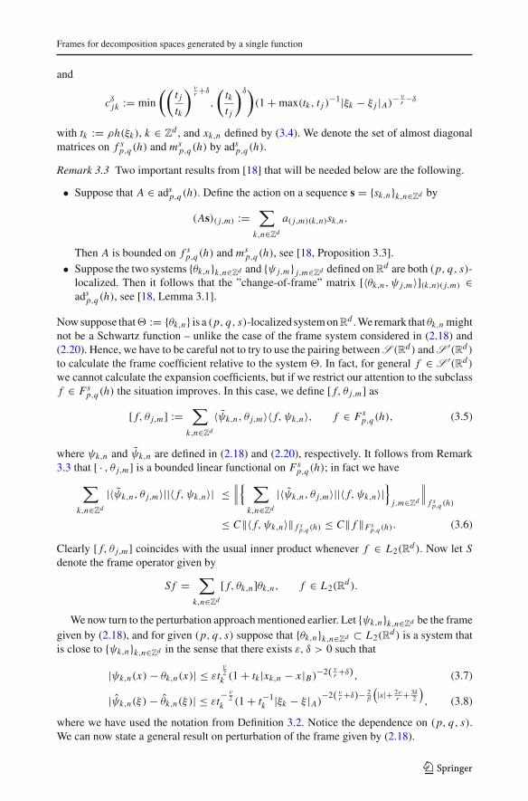
and

cδjk := min

((t j

tk

) νr +δ

,

(tkt j

)δ)(1 + max(tk, t j )

−1|ξk − ξ j |A)− ν

r −δ

with tk := ρh(ξk), k ∈ Zd , and xk,n defined by (3.4). We denote the set of almost diagonal

matrices on f sp,q(h) and ms

p,q(h) by adsp,q(h).

Remark 3.3 Two important results from [18] that will be needed below are the following.

• Suppose that A ∈ adsp,q(h). Define the action on a sequence s = {sk,n}k,n∈Zd by

(As)( j,m) :=∑

k,n∈Zd

a( j,m)(k,n)sk,n .

Then A is bounded on f sp,q(h) and ms

p,q(h), see [18, Proposition 3.3].

• Suppose the two systems {θk,n}k,n∈Zd and {ψ j,m} j,m∈Zd defined on Rd are both (p, q, s)-

localized. Then it follows that the ”change-of-frame” matrix [〈θk,n, ψ j,m〉](k,n)( j,m) ∈ads

p,q(h), see [18, Lemma 3.1].

Now suppose that� := {θk,n} is a (p, q, s)-localized system on Rd . We remark that θk,n might

not be a Schwartz function – unlike the case of the frame system considered in (2.18) and(2.20). Hence, we have to be careful not to try to use the pairing between S (Rd) and S ′(Rd)

to calculate the frame coefficient relative to the system �. In fact, for general f ∈ S ′(Rd)

we cannot calculate the expansion coefficients, but if we restrict our attention to the subclassf ∈ Fs

p,q(h) the situation improves. In this case, we define [ f, θ j,m] as

[ f, θ j,m] :=∑

k,n∈Zd

〈ψk,n, θ j,m〉〈 f, ψk,n〉, f ∈ Fsp,q(h), (3.5)

where ψk,n and ψk,n are defined in (2.18) and (2.20), respectively. It follows from Remark3.3 that [ · , θ j,m] is a bounded linear functional on Fs

p,q(h); in fact we have∑

k,n∈Zd

|〈ψk,n, θ j,m〉||〈 f, ψk,n〉| ≤∥∥∥{ ∑

k,n∈Zd

|〈ψk,n, θ j,m〉||〈 f, ψk,n〉|}

j,m∈Zd

∥∥∥f s

p,q (h)

≤ C‖〈 f, ψk,n〉‖ f sp,q (h) ≤ C‖ f ‖Fs

p,q (h). (3.6)

Clearly [ f, θ j,m] coincides with the usual inner product whenever f ∈ L2(Rd). Now let S

denote the frame operator given by

S f =∑

k,n∈Zd

[ f, θk,n]θk,n, f ∈ L2(Rd).

We now turn to the perturbation approach mentioned earlier. Let {ψk,n}k,n∈Zd be the framegiven by (2.18), and for given (p, q, s) suppose that {θk,n}k,n∈Zd ⊂ L2(R

d) is a system thatis close to {ψk,n}k,n∈Zd in the sense that there exists ε, δ > 0 such that

|ψk,n(x)− θk,n(x)| ≤ εtν2

k (1 + tk |xk,n − x |B)−2( νr +δ), (3.7)

|ψk,n(ξ)− θk,n(ξ)| ≤ εt− ν

2k (1 + t−1

k |ξk − ξ |A)−2( νr +δ)− 2

β

(|s|+ 2ν

r + 3δ2

), (3.8)

where we have used the notation from Definition 3.2. Notice the dependence on (p, q, s).We can now state a general result on perturbation of the frame given by (2.18).

123

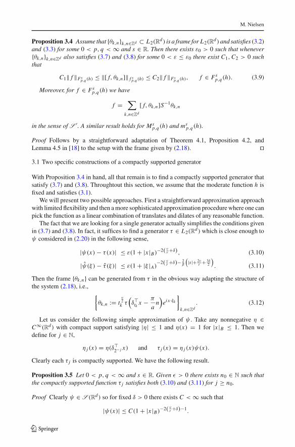
M. Nielsen

Proposition 3.4 Assume that {θk,n}k,n∈Zd ⊂ L2(Rd) is a frame for L2(R

d) and satisfies (3.2)and (3.3) for some 0 < p, q < ∞ and s ∈ R. Then there exists ε0 > 0 such that whenever{θk,n}k,n∈Zd also satisfies (3.7) and (3.8) for some 0 < ε ≤ ε0 there exist C1,C2 > 0 suchthat

C1‖ f ‖Fsp,q (h) ≤ ‖[ f, θk,n]‖ f s

p,q (h) ≤ C2‖ f ‖Fsp,q (h), f ∈ Fs

p,q(h). (3.9)

Moreover, for f ∈ Fsp,q(h) we have

f =∑

k,n∈Zd

[ f, θk,n]S−1θk,n

in the sense of S ′. A similar result holds for Msp,q(h) and ms

p,q(h).

Proof Follows by a straightforward adaptation of Theorem 4.1, Proposition 4.2, andLemma 4.5 in [18] to the setup with the frame given by (2.18). ��3.1 Two specific constructions of a compactly supported generator

With Proposition 3.4 in hand, all that remain is to find a compactly supported generator thatsatisfy (3.7) and (3.8). Throughtout this section, we assume that the moderate function h isfixed and satisfies (3.1).

We will present two possible approaches. First a straightforward approximation approachwith limited flexibility and then a more sophisticated approximation procedure where one canpick the function as a linear combination of translates and dilates of any reasonable function.

The fact that we are looking for a single generator actually simplifies the conditions givenin (3.7) and (3.8). In fact, it suffices to find a generator τ ∈ L2(R

d) which is close enough toψ considered in (2.20) in the following sense,

|ψ(x)− τ(x)| ≤ ε(1 + |x |B)−2( νr +δ), (3.10)

|ψ(ξ)− τ (ξ )| ≤ ε(1 + |ξ |A)−2( νr +δ)− 2

β

(|s|+ 2ν

r + 3δ2

). (3.11)

Then the frame {θk,n} can be generated from τ in the obvious way adapting the structure ofthe system (2.18), i.e., {

θk,n := tν2

k τ(δ�tk x − π

an)

eix ·ξk

}k,n∈Zd

. (3.12)

Let us consider the following simple approximation of ψ . Take any nonnegative η ∈C∞(Rd) with compact support satisfying |η| ≤ 1 and η(x) = 1 for |x |B ≤ 1. Then wedefine for j ∈ N,

η j (x) = η(δ�2− j x) and τ j (x) = η j (x)ψ(x).

Clearly each τ j is compactly supported. We have the following result.

Proposition 3.5 Let 0 < p, q < ∞ and s ∈ R. Given ε > 0 there exists n0 ∈ N such thatthe compactly supported function τ j satisfies both (3.10) and (3.11) for j ≥ n0.

Proof Clearly ψ ∈ S (Rd) so for fixed δ > 0 there exists C < ∞ such that

|ψ(x)| ≤ C(1 + |x |B)−2( νr +δ)−1.

123

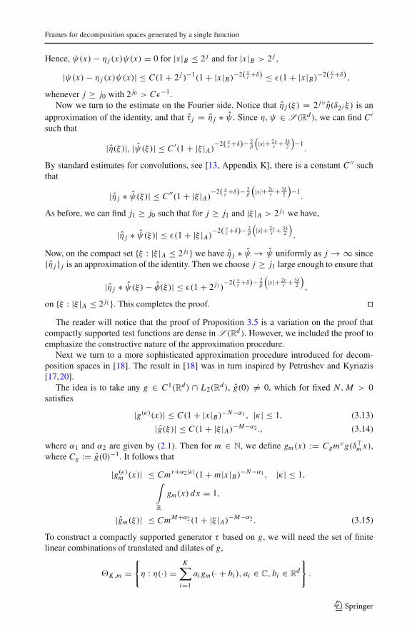
Frames for decomposition spaces generated by a single function

Hence, ψ(x)− η j (x)ψ(x) = 0 for |x |B ≤ 2 j and for |x |B > 2 j ,

|ψ(x)− η j (x)ψ(x)| ≤ C(1 + 2 j )−1(1 + |x |B)−2( νr +δ) ≤ ε(1 + |x |B)

−2( νr +δ),

whenever j ≥ j0 with 2 j0 > Cε−1.Now we turn to the estimate on the Fourier side. Notice that η j (ξ) = 2 jν η(δ2 j ξ) is an

approximation of the identity, and that τ j = η j ∗ ψ . Since η,ψ ∈ S (Rd), we can find C ′such that

|η(ξ)|, |ψ(ξ)| ≤ C ′(1 + |ξ |A)−2( νr +δ)− 2

β

(|s|+ 2ν

r + 3δ2

)−1.

By standard estimates for convolutions, see [13, Appendix K], there is a constant C ′′ suchthat

|η j ∗ ψ(ξ)| ≤ C ′′(1 + |ξ |A)−2( νr +δ)− 2

β

(|s|+ 2ν

r + 3δ2

)−1.

As before, we can find j1 ≥ j0 such that for j ≥ j1 and |ξ |A > 2 j1 we have,

|η j ∗ ψ(ξ)| ≤ ε(1 + |ξ |A)−2( νr +δ)− 2

β

(|s|+ 2ν

r + 3δ2

).

Now, on the compact set {ξ : |ξ |A ≤ 2 j1} we have η j ∗ ψ → ψ uniformly as j → ∞ since{η j } j is an approximation of the identity. Then we choose j ≥ j1 large enough to ensure that

|η j ∗ ψ(ξ)− φ(ξ)| ≤ ε(1 + 2 j1)−2( νr +δ)− 2

β

(|s|+ 2ν

r + 3δ2

),

on {ξ : |ξ |A ≤ 2 j1}. This completes the proof. ��The reader will notice that the proof of Proposition 3.5 is a variation on the proof that

compactly supported test functions are dense in S (Rd). However, we included the proof toemphasize the constructive nature of the approximation procedure.

Next we turn to a more sophisticated approximation procedure introduced for decom-position spaces in [18]. The result in [18] was in turn inspired by Petrushev and Kyriazis[17,20].

The idea is to take any g ∈ C1(Rd) ∩ L2(Rd), g(0) �= 0, which for fixed N ,M > 0

satisfies

|g(κ)(x)| ≤ C(1 + |x |B)−N−α1 , |κ| ≤ 1, (3.13)

|g(ξ)| ≤ C(1 + |ξ |A)−M−α2 ., (3.14)

where α1 and α2 are given by (2.1). Then for m ∈ N, we define gm(x) := Cgmνg(δ�m x),where Cg := g(0)−1. It follows that

|g(κ)m (x)| ≤ Cmν+α2|κ|(1 + m|x |B)−N−α1 , |κ| ≤ 1,∫

R

gm(x) dx = 1,

|gm(ξ)| ≤ CmM+α2(1 + |ξ |A)−M−α2 . (3.15)

To construct a compactly supported generator τ based on g, we will need the set of finitelinear combinations of translated and dilates of g,

�K ,m ={η : η(·) =

K∑i=1

ai gm(· + bi ), ai ∈ C, bi ∈ Rd

}.

123

M. Nielsen

We are now ready to show that any function with sufficient decay in both direct and frequencyspace can be approximated to an arbitrary degree by a finite linear combination of anotherfunction with similar decay.

Proposition 3.6 Let N ′ > N > ν and M ′ > M > ν. If g ∈ C1(Rd) ∩ L2(Rd), g(0) �= 0,

fulfills (3.13) and (3.14) and ψ ∈ C1(Rd) ∩ L2(Rd) fulfills

|ψ(x)| ≤ C(1 + |x |B)−N ′

,

|ψ(κ)(x)| ≤ C, |κ| ≤ 1,

|ψ(ξ)| ≤ C(1 + |ξ |A)−M ′

,

then for any ε > 0 there exists K ,m ≥ 1 and τ ∈ �K ,m such that

|ψ(x)− τ(x)| ≤ ε(1 + |x |B)−N , (3.16)

|ψ(ξ)− τ (ξ )| ≤ ε(1 + |ξ |A)−M . (3.17)

As before, the resulting frame is then given by (3.12).

Proof The proof is similar to the proof of Proposition 5.1 in [18]. ��3.2 Some concluding remarks on numerical calculations

There is one major advantage for numerical calculation to the construction given by Propo-sition 3.6; this is the fact that we can choose the initial function g as we please only subjectto some very mild constraints.

We can use this to make the final frame generated by τ from Proposition 3.6 better adaptedto numerical calculations. For example, we can choose g to be a compactly supported splineor a compactly supported orthonormal scaling function for a multiresolution analysis. Thenwe generate τ by Proposition 3.6. We can clearly write

τ =K∑

i=1

ai g(δmi · +bi ).

Then for any f ∈ L1,loc(Rd),

〈 f, τ 〉 =K∑

i=1ai m

−τi

∫Rd

f (δ�1/mix − δ�1/mi

bi )g(x) dx, (3.18)

and we can use the properties of g to estimate the integrals in (3.18). The same type ofreasoning applies to dilated, translated, and modulated versions of τ , so this way we canestimated any frame coefficient of the system (3.12) generated by τ .

References

1. Borup, L., Nielsen, M.: Banach frames for multivariate α-modulation spaces. J. Math. Anal. Appl. 321(2),880–895 (2006)

2. Borup, L., Nielsen, M.: Nonlinear approximation in α-modulation spaces. Math. Nachr. 279(1–2), 101–120 (2006)

3. Borup, L., Nielsen, M.: Frame decomposition of decomposition spaces. J. Fourier Anal. Appl. 13(1),39–70 (2007)

4. Borup, L., Nielsen, M.: On anisotropic Triebel–Lizorkin type spaces, with applications to the study ofpseudo-differential operators. J. Funct. Spaces Appl. 6(2), 107–154 (2008)

123

Frames for decomposition spaces generated by a single function

5. Dahlke, S., Kutyniok, G., Steidl, G., Teschke, G.: Shearlet coorbit spaces and associated Banach frames.Appl. Comput. Harmon. Anal. 27(2), 195–214 (2009)

6. Dahlke, S., Steidl, G., Teschke, G.: The continuous shearlet transform in arbitrary space dimensions. J.Fourier Anal. Appl. 16(3), 340–364 (2010)

7. Feichtinger, H.G.: Banach spaces of distributions defined by decomposition methods. II. Math. Nachr.132, 207–237 (1987)

8. Feichtinger, H.G.: Modulation spaces of locally compact abelian groups. In: Radha, R., Krishna, M.,Thangavelu, S. (eds) Proceedings of International Conference on Wavelets and Applications, pp 1–56.Allied Publishers, New Delhi (2003)

9. Feichtinger, H.G., Fornasier, M.: Flexible Gabor-wavelet atomic decompositions for L2-Sobolev spaces.Ann. Mat. Pura Appl. (4), 185(1), 105–131 (2006)

10. Feichtinger, H.G., Gröbner, P.: Banach spaces of distributions defined by decomposition methods. I. Math.Nachr. 123, 97–120 (1985)

11. Fornasier, M.: Banach frames for α-modulation spaces. Appl. Comput. Harmon. Anal. 22(2), 157–175(2007)

12. Fornasier, M., Rauhut, H.: Continuous frames, function spaces, and the discretization problem. J. FourierAnal. Appl. 11(3), 245–287 (2005)

13. Grafakos, L.: Classical and Modern Fourier Analysis, 1st edn. Pearson Education, New Jersey (2004)14. Gröbner, P.: Banachräume glatter Funktionen und Zerlegungsmethoden. PhD thesis, University of Vienna

(1992)15. Grohs, P.: Continuous shearlet frames and resolution of the wavefront set. Monatsh. Math. 164(4), 393–

426 (2011)16. Grohs, P.: Ridgelet-type frame decompositions for Sobolev spaces related to linear transport. J. Fourier

Anal. Appl. 18(2), 309–325 (2012)17. Kyriazis, G., Petrushev, P.: New bases for Triebel–Lizorkin and Besov spaces. Trans. Am. Math. Soc.

354(2), 749–776 (electronic) (2002)18. Nielsen, M., Rasmussen, K.: Compactly supported frames for decomposition spaces. J. Fourier Anal.

Appl. 18, 87–117 (2012). doi:10.1007/s00041-011-9190-519. Päivärinta, L., Somersalo, E.: A generalization of the Calderón-Vaillancourt theorem to L p and h p . Math.

Nachr. 138, 145–156 (1988)20. Petrushev, P.: Bases consisting of rational functions of uniformly bounded degrees or more general

functions. J. Funct. Anal. 174(1), 18–75 (2000)21. Rauhut, H., Ullrich, T.: Generalized coorbit space theory and inhomogeneous function spaces of Besov–

Lizorkin–Triebel type. J. Funct. Anal. 260(11), 3299–3362 (2011)22. Romero, J.L.: Characterization of coorbit spaces with phase-space covers. J. Funct. Anal. 262(1), 59–93

(2012)23. Stein, E.M.: Harmonic analysis: real-variable methods, orthogonality, and oscillatory integrals, volume

43 of Princeton Mathematical Series. Princeton University Press, Princeton, NJ, : With the assistance ofTimothy S. Murphy, Monographs in Harmonic Analysis, III (1993)

24. Stein, E.M., Wainger, S.: Problems in harmonic analysis related to curvature. Bull. Am. Math. Soc. 84(6),1239–1295 (1978)

25. Triebel, H.: Theory of function spaces, volume 78 of Monographs in Mathematics. Birkhäuser Verlag,Basel (1983)

123