Embed Size (px)
Citation preview
Found Comput Math (2018) 18:757–788https://doi.org/10.1007/s10208-017-9353-0
Interpolation on Symmetric Spaces Via the GeneralizedPolar Decomposition
Evan S. Gawlik1 · Melvin Leok1
Received: 21 May 2016 / Revised: 29 March 2017 / Accepted: 4 May 2017 /Published online: 26 May 2017© SFoCM 2017
Abstract We construct interpolation operators for functions taking values in a sym-metric space—a smooth manifold with an inversion symmetry about every point. Keyto our construction is the observation that every symmetric space can be realized asa homogeneous space whose cosets have canonical representatives by virtue of thegeneralized polar decomposition—a generalization of the well-known factorizationof a real nonsingular matrix into the product of a symmetric positive-definite matrixtimes an orthogonal matrix. By interpolating these canonical coset representatives, wederive a family of structure-preserving interpolation operators for symmetric space-valued functions. As applications, we construct interpolation operators for the space ofLorentzian metrics, the space of symmetric positive-definite matrices, and the Grass-mannian. In the case ofLorentzianmetrics, our interpolation operators provide a familyof finite elements for numerical relativity that are frame-invariant and have signaturewhich is guaranteed to be Lorentzian pointwise. We illustrate their potential utility byinterpolating the Schwarzschild metric numerically.
Keywords Interpolation · Manifold-valued data · Symmetric space · Generalizedpolar decomposition ·Grassmannian · Lorentzian metric · Lie triple system ·Geodesicfinite element · Karcher mean · Log-Euclidean mean
Communicated by Arieh Iserles.
B Evan S. [email protected]
Melvin [email protected]
1 Department of Mathematics, University of California, San Diego,9500 Gilman Drive #0112, La Jolla, CA 92093-0112, USA
123
758 Found Comput Math (2018) 18:757–788
Mathematics Subject Classification Primary 65D05 · 53C35; Secondary 65N30 ·58J70 · 53B30
1 Introduction
Manifold-valued data and manifold-valued functions play an important role in a widevariety of applications, including mechanics [14,24,42], computer vision and graph-ics [11,13,15,18–20,30,32,47], medical imaging [7], and numerical relativity [5]. Bytheir very nature, such applications demand that care be takenwhenperforming compu-tations thatwould otherwise be routine, such as averaging, interpolation, extrapolation,and the numerical solution of differential equations. This paper constructs interpola-tion and averaging operators for functions taking values in a symmetric space—asmooth manifold with an inversion symmetry about every point. Key to our construc-tion is the observation that every symmetric space can be realized as a homogeneousspace whose cosets have canonical representatives by virtue of the generalized polardecomposition—ageneralization of the well-known factorization of a real nonsingularmatrix into the product of a symmetric positive-definite matrix times an orthogonalmatrix. By interpolating these canonical coset representatives, we derive a family ofstructure-preserving interpolation operators for symmetric space-valued functions.
Our motivation for constructing such operators is best illustrated by example.Among themost interesting scenarios inwhich symmetric space-valued functions playa role is numerical relativity. There, the dependent variable in Einstein’s equations—the metric tensor—is a function taking values in the space L of Lorentzian metrics:symmetric, nondegenerate 2-tensors with signature (3, 1). This space is neither a vec-tor space nor a convex set. Rather, it has the structure of a symmetric space. As aconsequence, the outputs of basic arithmetic operations on Lorentzian metrics such asaveraging, interpolation, and extrapolation need not remain in L. This is undesirablefor several reasons. If the metric tensor field is to be discretized with finite elements,then a naive approach in which the components of the metric are discretized withpiecewise polynomials may fail to produce a metric field with signature (3, 1) at allpoints in space-time. Perhaps an even more problematic possibility is that a numericaltime integrator used to advance the metric forward in time (e.g., in a 3+1 formulationof Einstein’s equations) might produce metrics with invalid signature. One of the aimsof the present paper is to avert these potential dangers altogether by constructing astructure-preserving interpolation operator for Lorentzian metrics. As will be shown,the interpolation operator we derive not only produces interpolants that everywherebelong to L, but it is also frame-invariant: the interpolation operator we derive com-mutes with the action of the indefinite orthogonal group O(1, 3) on L. Furthermore,our interpolation operator commutes with inversion and interpolates the determinantof the metric tensor in a monotonic manner.
A more subtle example is the space SPD(n) of symmetric positive-definite n × nmatrices. This space forms a convex cone, so arithmetic averaging and linear interpo-lation trivially produce SPD(n)-valued results. Nevertheless, these operations fail topreserve other structures that are important in some applications. For instance, arith-metic averaging does not commute with matrix inversion, and the determinant of the
123
Found Comput Math (2018) 18:757–788 759
arithmetic average need not be less than or equal to the maximum of the determinantsof the data. This may remedied by considering instead the Riemannian mean (alsoknown as the Karcher mean) of symmetric positive-definite matrices with respect tothe canonical left-invariantRiemannianmetric on SPD(n) [9,33,38]. TheRiemannianmean cannot, in general, be expressed in closed form, but it can be computed iterativelyand possesses a number of structure-preserving properties; see [9] for details. A lesscomputationally expensive alternative, introduced by Arsigny et al. [6], is to computethe mean of symmetric positive-definite matrices with respect to a log-Euclidean met-ric on SPD(n). The resulting averaging operator commutes with matrix inversion,prevents overestimation of the determinant, and commutes with similarity transfor-mations that consist of an isometry plus scaling. Both of these constructions turn outto be special cases of the general theory presented in this paper. In our derivation ofthe log-Euclidean mean, we give a clear geometric explanation of the vector spacestructure with which Arsigny et al. [6] endow SPD(n) in their derivation, which turnsout to be nothing more than a correspondence between a symmetric space (SPD(n))and a Lie triple system [25].
Another symmetric space which we address in this paper is the GrassmannianGr(p, n), which consists of all p-dimensional linear subspaces of Rn . Interpolationon theGrassmannian is a task of importance in a variety of contexts, including reduced-order modeling [4,48] and computer vision [13,19,30,47]. Not surprisingly, this taskhas received much attention in the literature; see [2,8] and the references therein. Ourconstructions in this paper recover some of the well-known interpolation schemes onthe Grassmannian, including those that appear in [4,8,13].
There are connections between the present work and geodesic finite elements [21,22,43,44], a family of conforming finite elements for functions taking values in aRiemannian manifold M . In fact, we recover such elements as a special case; seeSect. 3.3. Since their evaluation amounts to the computation of aweighted Riemannianmean, geodesic finite elements and their derivatives can sometimes be expensive tocompute. One of themessages we hope to convey is that whenM is a symmetric space,this additional structure enables the construction of alternative interpolants that areless expensive to compute but still possess many of the desirable features of geodesicfinite elements.
Our use of the generalized polar decomposition in this paper is inspired by a streamof research [31,40,41] that has, in recent years, cast a spotlight on the generalizedpolar decomposition’s role in numerical analysis. Much of our exposition and notationparallels that which appears in those papers, and we encourage the reader to look therefor further insight.
Some of the key contributions of this paper include the following. First, the paperunifies several seemingly disparate interpolation strategies, some of which have beenderived in an ad hoc way in the literature. The paper also unveils the geometricunderpinnings of these interpolants’ structure-preserving properties. These structure-preserving properties are unique to symmetric spaces and lead to important practicalconsequences, including frame-invariance in the context of Lorentzian metric inter-polation. On the practical side, the paper also shows that symmetric spaces admitefficiently computable interpolants. This is significant, since on a general Riemannianmanifold M , for instance, it is a simple matter to write down interpolation schemes
123
760 Found Comput Math (2018) 18:757–788
for M-valued data using the Riemannian exponential map and its inverse, but it isgenerally not the case that the exponential map can be calculated explicitly, much lessinverted. We show that for a symmetric space S, these tasks are tractable. Our use ofthe generalized polar decomposition plays a key role here, since it reveals not onlyhow to construct a map from a linear space to S, but also how to systematically invertit, a task which would otherwise be nontrivial except in special cases. We also deriveformulas for the first and second derivatives of the resulting interpolants. Finally, toour knowledge, the paper introduces the first structure-preserving finite elements forLorentzian metrics in numerical relativity.
Organization. This paper is organized as follows. We begin in Sect. 2 by reviewingsymmetric spaces, Lie triple systems, and the generalized polar decomposition. Then,in Sect. 3, we exploit a correspondence between symmetric spaces and Lie triplesystems to construct interpolation operators on symmetric spaces. Finally, in Sect. 4,we specialize these interpolation operators to three examples of symmetric spaces: thespace of symmetric positive-definite matrices, the space of Lorentzian metrics, and theGrassmannian. In the case of Lorentzian metrics, we illustrate the potential utility ofthese interpolation operators by interpolating the Schwarzschild metric numerically.
2 Symmetric Spaces and the Generalized Polar Decomposition
In this section, we review symmetric spaces, Lie triple systems, and the generalizedpolar decomposition. We describe a well-known correspondence between symmetricspaces and Lie triple systems that will serve in Sect. 3 as a foundation for interpolatingfunctions which take values in a symmetric space. For further background material,we refer the reader to [25,40,41,49].
2.1 Notation and Definitions
Let G be a Lie group and let σ : G → G be an involutive automorphism. That is,σ �= id. is a bijection satisfying σ(σ(g)) = g and σ(gh) = σ(g)σ (h) for everyg, h ∈ G. Denote by Gσ the subgroup of G consisting of fixed points of σ :
Gσ = {g ∈ G | σ(g) = g}.
Suppose that G acts transitively on a smooth manifold S with a distinguished elementη ∈ S whose stabilizer coincides with Gσ . In other words,
g · η = η ⇐⇒ σ(g) = g,
where g · u denotes the action of g ∈ G on an element u ∈ S. Then there is a bijectivecorrespondence between elements of the homogeneous space G/Gσ and elements ofS. On the other hand, the cosets in G/Gσ have canonical representatives by virtueof the generalized polar decomposition [40,41]. This decomposition states that anyg ∈ G sufficiently close to the identity e ∈ G can be written as a product
123
Found Comput Math (2018) 18:757–788 761
g = pk, p ∈ Gσ , k ∈ Gσ , (1)
where
Gσ = {g ∈ G | σ(g) = g−1}.Moreover, this decomposition is unique in the neighborhood of e onwhich it exists [41,Theorem 3.1]. As a consequence, there is a bijection between a neighborhood in Gσ
of the identity e ∈ Gσ and a neighborhood of the coset [e] ∈ G/Gσ . The spaceGσ—which, unlikeGσ , is not a subgroup ofG—is a symmetric space which is closedunder a nonassociative symmetric product g · h = gh−1g. Its tangent space at theidentity is the space
p = {Z ∈ g | dσ(Z) = −Z}.Here, g denotes the Lie algebra of G, and dσ : g → g denotes the differential of σ ate, which can be expressed in terms of the Lie group exponential map exp : g → Gvia
dσ(Z) = d
dt
∣∣∣∣t=0
σ(exp(t Z)).
The space p, which is not a Lie subalgebra of g, has the structure of a Lie triple system:it is a vector space closed under the double commutator [·, [·, ·]]. In contrast, the space
k = {Z ∈ g | dσ(Z) = Z}is a subalgebra of g, as it is closed under the commutator [·, ·]. This subalgebra isnone other than the Lie algebra of Gσ . The generalized polar decomposition (1) hasa manifestation at the Lie algebra level called the generalized Cartan decomposition,which decomposes g as a direct sum
g = p ⊕ k. (2)
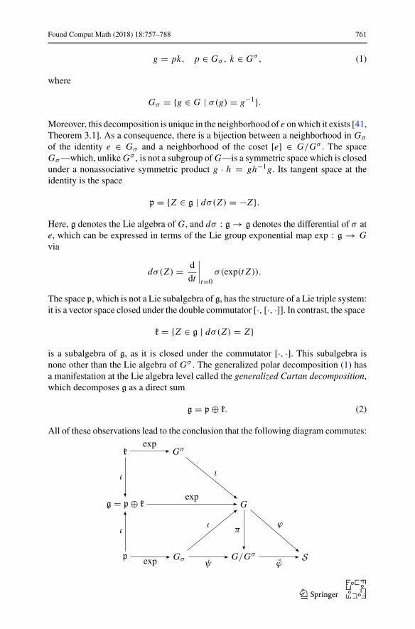
All of these observations lead to the conclusion that the following diagram commutes:
G
G/GσGσ Sp
g = p ⊕ k
k Gσ
πϕ
ϕψ
ι
exp
ι
exp
ι
exp
ι
123
762 Found Comput Math (2018) 18:757–788
In this diagram, we have used the letter ι to denote the canonical inclusion, π :G → G/Gσ the canonical projection, and ϕ : G → S the map ϕ(g) = g · η. Themaps ψ and ϕ are defined by the condition that the diagram be commutative.
2.2 Correspondence Between Symmetric Spaces and Lie Triple Systems
An important feature of the diagram above is that the maps along its bottom row—when restricted to suitable neighborhoods of the neutral elements 0 ∈ p, e ∈ Gσ ,[e] ∈ G/Gσ , and the distinguished element η ∈ S—are diffeomorphisms [25, p. 104,p. 124, p. 253]. In particular, the composition
F = ϕ ◦ ψ ◦ exp (3)
(or, equivalently, F = ϕ ◦ ι ◦ exp) provides a diffeomorphism from a neighborhoodof 0 ∈ p to a neighborhood of η ∈ S, given by
F(P) = exp(P) · η
for P ∈ p. The space p, being a vector space, offers a convenient space to performcomputations (such as averaging, interpolation, extrapolation, and the numerical solu-tion of differential equations) that might otherwise be unwieldy on the space S. Thisis analogous to the situation that arises when working with the Lie group G. Often,computations on G are more easily performed by mapping elements of G to the Liealgebra g via the inverse of the exponential map (or an approximation thereof), per-forming computations in g, and mapping the result back to G via the exponential map(or an approximation thereof).
We remark that the analogy just drawn between computing on Lie groups andcomputing on symmetric spaces is in fact more than a mere resemblance; the lattersituation directly generalizes the former. Indeed, any Lie group G can be realized as asymmetric space by considering the action ofG×G onG given by (g, h)·k = gkh−1.The stabilizer of e ∈ G is the diagonal of G × G, which is precisely the subgroupfixed by the involution σ(g, h) = (h, g). In this setting, one finds that the map (3)takes (X,−X) ∈ g× g to exp(2X) ∈ G. This shows that, up to a trivial modification,the map (3) reduces to the Lie group exponential map if S happens to be a Lie group.
An additional feature of the map (3) is its equivariance with respect to the actionof Gσ on S and p. Specifically, for g ∈ G, let Adg : g → g denote the adjoint actionof G on g:
Adg Z = d
dt
∣∣∣∣t=0
g exp(t Z)g−1.
In a slight abuse of notation, we will write
Adg Z = gZg−1
123
Found Comput Math (2018) 18:757–788 763
in this paper, bearing in mind that the above equality holds in the sense of matrixmultiplication for anymatrix group. The following lemma shows that F◦Adg
∣∣p
= g·Ffor every g ∈ Gσ . Note that this statement makes implicit use of the (easily verifiable)fact that Adg leaves p invariant when g ∈ Gσ ; that is, gPg−1 ∈ p for every g ∈ Gσ
and every P ∈ p.
Lemma 2.1 For every P ∈ p and every g ∈ Gσ ,
g · F(P) = F(gPg−1).
Proof Note that g ∈ Gσ implies g−1 ∈ Gσ , so g−1 · η = η. Hence, sinceexp(gPg−1) = g exp(P)g−1,
F(gPg−1) = exp(gPg−1) · η
= g exp(P)g−1 · η
= g exp(P) · η
= g · F(P)
We finish this section by remarking that σ induces a family of symmetries on S as
follows. Define sη : S → S by setting
sη(g · η) = σ(g) · η
for each g ∈ G. Note that sη is well defined, fixes η, and has differential equal tominus the identity. Furthermore, by definition, the following diagram commutes:
p
p
G
G
S
S
exp
exp
ϕ
ϕ
dσ σ sη
Written another way,sη(F(P)) = F(−P) (4)
for every P ∈ p. In a similar manner, a symmetry at each point h · η ∈ S can bedefined via
sh·η(g · η) = h · sη(h−1g · η) = hσ(h−1g) · η.
If S admits a G-invariant Riemannian metric, then the maps F and sh·η have par-ticularly notable interpretations. Any such metric induces a canonical connection onS [35, Thoerem 3.3]. With respect to this connection, F may be identified with the
123
764 Found Comput Math (2018) 18:757–788
Riemannian exponential map Expη : TηS → S upon identifying p with TηS viap ∼= g/k = T[e](G/Gσ ) ∼= TηS [35, Theorem 3.2(3)]. In addition, the map sh·η is anisometry that sends Exph·η(X) to Exph·η(−X) for every X ∈ Th·ηS [35, p. 231]. Asan important special case, note that S admits a G-invariant Riemannian metric when-ever Gσ is compact [35, p. 245]. Examples of symmetric spaces that do not admitG-invariant Riemannian metrics include the space of symmetric 4 × 4 matrices withsignature (3, 1) (see Sect. 4.1.2) and the affine Grassmannian manifold consisting ofp-dimensional affine subspaces of Rn [49, Section 7.5].
2.3 Generalizations
The construction above can be generalized by replacing the exponential map in (3)with a different local diffeomorphism. One example is given by fixing an elementg ∈ G and replacing exp : p → Gσ in (3) with the map
P �→ ψ−1 ([g exp(P)]) = ψ−1(π(g exp(P))). (5)
The output of this map is nothing more than the factor p in the generalized polardecomposition g exp(P) = pk, p ∈ Gσ , k ∈ Gσ . The map (3) then becomes
Fg(P) = g exp(P) · η. (6)
This generalization of (3) has the property that it provides a diffeomorphism betweena neighborhood of 0 ∈ p and a neighborhood of g · η ∈ S rather than η. Note thatwhen g = e (the identity element), this map coincides with (3). A calculation similarto the proof of Lemma 2.1 shows that the map (g, P) �→ Fg(P) is Gσ -equivariant, inthe sense that
Fhgh−1(hPh−1) = h · Fg(P) (7)
for every h ∈ Gσ and every P ∈ p. Furthermore,
sg·η(Fg(P)) = Fg(−P) (8)
for every P ∈ p. These identities are summarized in the following pair of diagrams,the first of which commutes for every h ∈ Gσ , and the second of which commutes forevery g ∈ G.
G × p
G × p
S
S
f
f
�h h
p
p
S
S
Fg
Fg
dσ sg·η
123
Found Comput Math (2018) 18:757–788 765
Here, we have denoted f (g, P) = Fg(P), �h(g, P) = (hgh−1, hPh−1), andh(u) = h · u.
More generally, one may consider replacing the exponential map in (5) with anyretraction R : g → G [1, p. 55]. For instance, if G is a quadratic matrix group, onemay choose R equal to the Cayley transform, or more generally, any diagonal Padéapproximant of the matrix exponential [12].
3 Interpolation on Symmetric Spaces
In this section, we exploit the correspondence between symmetric spaces and Lie triplesystems discussed in Sects. 2.2–2.3 in order to interpolate functions which take valuesin a symmetric space.
3.1 A Structure-Preserving Interpolant
Consider the task of interpolating m elements u1, u2, . . . , um ∈ S. To facilitate theexposition, we will think of these elements as the values of a smooth function u : → S defined on a domain ⊂ R
d , d ≥ 1, at locations x (1), x (2), . . . , x (m) ∈ ,although this point of view is not essential in what follows. Our goal is thus to constructa function Iu : → S that satisfies Iu(x (i)) = ui , i = 1, 2, . . . ,m, and has a desiredlevel of regularity (e.g., continuity). We assume that for each x ∈ , u(x) belongsto the range of map (3). We may then interpolate u1, u2, . . . , um by interpolatingF−1(u1), F−1(u2), . . . , F−1(um) ∈ p and mapping the result back to S via F . Moreprecisely, set
Iu(x) = F(IP(x)), (9)
where P(x) = F−1(u(x)) and IP : → p is an interpolant of F−1(u1), F−1(u2),. . . , F−1(um). Then Iu interpolates the data while fulfilling the following importantproperties.
Proposition 3.1 Suppose that I commutes with Adg for every g ∈ Gσ . That is,
I(gPg−1)(x) = gIP(x)g−1
for every x ∈ and every g ∈ Gσ . Then I is Gσ -equivariant. That is,
I(g · u)(x) = g · Iu(x) (10)
for every x ∈ and every g ∈ Gσ sufficiently close to the identity.
Proof The claim is a straightforward consequence of Lemma 2.1.
Note that g must be sufficiently close to the identity in (10) to ensure that g · uibelongs to the range of the map (3) for each i = 1, 2, . . . ,m.
123
766 Found Comput Math (2018) 18:757–788
Proposition 3.2 Suppose that I commutes with dσ∣∣p. That is,
I(−P)(x) = −IP(x)
for every x ∈ . Then I commutes with sη. That is,
I(sη(u))(x) = sη(Iu(x))
for every x ∈ .
Proof The claim is a straightforward consequence of (4). The preceding propositions apply, in particular, to any interpolant IP : → p of
the form
IP(x) =m∑
i=1
φi (x)P(x (i))
with scalar-valued shape functions φi : → R, i = 1, 2, . . . ,m, satisfyingφi (x ( j)) = δi j , where δi j denotes the Kronecker delta. By the propositions above,such an interpolant gives rise to a Gσ -equivariant interpolant Iu : → S thatcommutes with sη, given by
Iu(x) = F
(m∑
i=1
φi (x)F−1(ui )
)
. (11)
Written more explicitly,Iu(x) = exp(IP(x)) · η, (12)
where
IP(x) =m∑
i=1
φi (x)F−1(ui ). (13)
Note that the interpolation strategy above resembles the ones used in, for instance,[6,16,23,50].
3.2 Derivatives of the Interpolant
The relations (12–13) lead to an explicit formula for the derivatives of Iu(x) withrespect to each of the coordinate directions x j , j = 1, 2, . . . , d. Namely,
∂Iu∂x j
(x) = dexpIP(x)
∂IP∂x j
(x) · η, (14)
123
Found Comput Math (2018) 18:757–788 767
where
∂IP∂x j
(x) =m∑
i=1
∂φi
∂x j(x)F−1(ui )
and dexpXY denotes the differential of exp at X ∈ g in the direction Y ∈ g.An explicit formula for dexpXY is the series
dexpXY = exp(X)
∞∑
k=0
(−1)k
(k + 1)!adkXY,
where adXY = [X,Y ] denotes the adjoint action of g on itself [29, p. 55]. In practice,one may truncate this series to numerically approximate dexpXY . Note that whilethe exact value of dexpXY belongs to p whenever X,Y ∈ p, this need not be trueof its truncated approximation. However, this is of little import since any spuriousk-components in such a truncation act trivially on η in (14).
While the series expansion of dexpXY is valid on any finite-dimensional Lie group,more efficient methods are available for the computation of dexpXY when G is amatrix group. Arguably, the simplest is to make use of the identity [26,37, p. 253]
exp
(
X Y0 X
)
=(
exp(X) dexpXY0 exp(X)
)
. (15)
More sophisticated approaches with better numerical properties can be found in [3,26,pp. 253–259].
The identity (15) can be leveraged to derive formulas for higher-order derivativesof Iu(x), provided of course that G is a matrix group. As shown in Appendix A, wehave
∂2Iu∂x j∂xk
(x) = A · η (16)
for each j, k = 1, 2, . . . , d, where A denotes the (1, 4) block of the matrix
exp
⎛
⎜⎜⎝
X Y Z W0 X 0 Z0 0 X Y0 0 0 X
⎞
⎟⎟⎠
,
and X = IP(x), Y = ∂IP∂x j
(x), Z = ∂IP∂xk
(x), and W = ∂2IP∂x j ∂xk
(x).
3.3 Generalizations
More generally, by fixing an element g ∈ G and adopting map (6) instead of F , weobtain interpolation schemes of the form
123
768 Found Comput Math (2018) 18:757–788
Igu(x) = Fg
(m∑
i=1
φi (x)F−1g (ui )
)
= g exp
(m∑
i=1
φi (x)F−1g (ui )
)
· η. (17)
Here, we must of course assume that ui belongs to the range of Fg for each i =1, 2, . . . ,m. This interpolant is therefore suitable for interpolating elements of S in aneighborhood of g ·η. Using the fact that Fhg(P) = h · Fg(P) for every h, g ∈ G andevery P ∈ p, one finds that this interpolant is equivariant under the action of the fullgroup G, in the sense that
Ihg(h · u)(x) = h · Igu(x) (18)
for every x ∈ and every h ∈ G sufficiently close to the identity. On the other hand,the equivariance of Fg under the action of the subgroup Gσ [recall (7)] implies that
Ihgh−1(h · u)(x) = h · Igu(x) (19)
for every x ∈ and every h ∈ Gσ sufficiently close to the identity. Comparing(18) with (19) leads to the conclusion that this interpolant is invariant under post-multiplication of g by elements of Gσ ; that is,
Ighu(x) = Igu(x) (20)
for every x ∈ and every h ∈ Gσ sufficiently close to the identity. Finally, as aconsequence of (8),
Ig(sg·η(u))(x) = sg·η(Igu(x))
for every x ∈ .A natural choice for g is not immediately evident, but one heuristic is to select
j ∈ {1, 2, . . . ,m} and set g equal to a representative of the coset ϕ−1(u j ). A moreinteresting option is to allow g to vary with x and to define g(x) implicitly via
g(x) · η = Ig(x)u(x). (21)
Equivalently,m∑
i=1
φi (x)F−1g(x)(ui ) = 0. (22)
A method for computing the interpolant Ig(x)u(x) numerically is self-evident.Namely, one performs the fixed-point iteration suggested by (21), as we explain ingreater detail in Sect. 4.
In what follows, we show that if Gσ is compact, so that S admits a G-invariantRiemannian metric, then (22) characterizes g(x) · η ∈ S as the weighted Riemannianmean of u1, u2, . . . , um . Recall that in this setting, the map F : p → S sending P to
123
Found Comput Math (2018) 18:757–788 769
exp(P) · η may be identified with the Riemannian exponential map Expη : TηS → Supon identifying p with TηS.Lemma 3.3 Suppose that Gσ is compact, so that S admits a G-invariant Riemannianmetric. If g(x) ∈ G is a solution of (21) [or, equivalently, (22)], then g(x) · η ∈ Slocally minimizes
m∑
i=1
φi (x) dist (g(x) · η, ui )2 (23)
among elements of S, where dist : S × S → R denotes the geodesic distance on S.Proof For each i = 1, 2, . . . ,m, let Pi = F−1
g(x)(ui ), so that g(x) exp(Pi ) · η = ui .Since the metric on S is G-invariant, the identity exp(Pi ) · η = Expη(Pi ) implies that
ui = g(x) · Expη(Pi ) = Expg(x)·η(g(x)Pi ). Equivalently, Pi = g(x)−1Exp−1g(x)·ηui .
This shows that (22) is equivalent to
m∑
i=1
φi (x)Exp−1g(x)·ηui = 0.
The latter equation is precisely the equation which characterizes minimizers of (23);see [33, Theorem 1.2].
Notice that minimizers of (23) are precisely geodesic finite elements on G/Gσ , asdescribed in [21,22,43,44].We refer the reader to those articles for further informationabout the approximation properties of these interpolants, as well as the convergenceproperties of iterative algorithms used to compute them.
3.4 Interpolation Error Estimates
Error estimates for interpolants of the form (9) can be derived by appealing to thesmoothness of the map F : p → S and the approximation properties of IP . Roughlyspeaking, the interpolant (9) inherits the approximation properties enjoyed by IPunder mild assumptions. To see this, consider the setting in which S is embedded inRn for some n ≥ 1. Denote by Du ∈ R
n×d and DF ∈ Rn×n the matrices of partial
derivatives of u and F , viewed as maps from ⊂ Rd and p � R
n , respectively, toRn . Define DP ∈ R
n×d , DIP ∈ Rn×d , and DIu ∈ R
n×d similarly. Our goal in whatfollows is to bound the norms of Iu(x)−u(x) and DIu(x)− Du(x) at a point x ∈
by the norms of IP(x) − P(x) and DIP(x) − DP(x). We use ‖ · ‖ to denote anyvector norm (when the argument is a vector) and the corresponding induced matrixnorm (when the argument is a matrix).
Proposition 3.4 Assume that DP is bounded on , and assume that F and DF areLipschitz on a set U ⊂ p whose interior contains the closure of P() = {P(x) | x ∈}. Define
123
770 Found Comput Math (2018) 18:757–788
C0 = supx∈
‖DP(x)‖,
C1 = supA,B∈UA �=B
‖F(A) − F(B)‖‖A − B‖ ,
C2 = supA,B∈UA �=B
‖DF(A) − DF(B)‖‖A − B‖ .
If supx∈ ‖IP(x) − P(x)‖ is sufficiently small, then for every x ∈ ,
‖Iu(x) − u(x)‖ ≤ C1‖IP(x) − P(x)‖ (24)
and
‖DIu(x) − Du(x)‖ ≤ C1‖DIP(x) − DP(x)‖+ C2‖IP(x) − P(x)‖
(
C0 + ‖DIP(x) − DP(x)‖)
. (25)
Proof If supx∈ ‖IP(x) − P(x)‖ is sufficiently small, then IP() = {IP(x) | x ∈} ⊆ U . Inequality (24) then follows immediately from the definition of C1, sinceIu = F ◦ IP and u = F ◦ P . Moreover, the chain rule implies
DIu(x) − Du(x) = DF(IP(x))DIP(x) − DF(P(x))DP(x)
=[
DF(IP(x)) − DF(P(x))]
DIP(x)
+ DF(P(x))[
DIP(x) − DP(x)]
.
Hence, noting that ‖DF(P(x))‖ ≤ C1, we have
‖DIu(x) − Du(x)‖ ≤ C2‖IP(x) − P(x)‖‖DIP(x)‖ + C1‖DIP(x) − DP(x)‖.
This proves inequality (25), since
‖DIP(x)‖ ≤ ‖DIP(x) − DP(x)‖ + ‖DP(x)‖≤ ‖DIP(x) − DP(x)‖ + C0.
The preceding proposition implies that the error in Iu is controlled pointwise by
the error in IP , and the error in DIu is controlled pointwise by the error in DIP ,up to the addition of terms that are, in typical applications, small in comparison withDIP − DP . Needless to say, analogous estimates with obvious modifications holdfor the interpolant (17).
123
Found Comput Math (2018) 18:757–788 771
It should be noted that these estimates depend on the choice of embedding of S inRn . Inequality (24) can be easily expressed more intrinsically by replacing the left-
hand side with the geodesic distance between Iu(x) and u(x), and replacing C1 withthe appropriately modified Lipschitz constant. Intrinsic variants of inequality (25) arenot as easy to derive, and it would be interesting to do so following the lead of [22]and [21].
4 Applications
In this section, we apply the general theory above to several symmetric spaces, includ-ing the space of symmetric positive-definite matrices, the space of Lorentzian metrics,and the Grassmannian.
4.1 Symmetric Matrices with Fixed Signature
Let n be a positive integer and let p and q be nonnegative integers satisfying p+q = n.Consider the set
L = {L ∈ GLn(R) | signature(L) = (q, p)},
where signature(L) denotes the signature of a nonsingular symmetric matrix L—anordered pair indicating the number of positive and negative eigenvalues of L . Thegeneral linear group GLn(R) acts transitively on L via the group action
A · L = ALAT ,
where A ∈ GLn(R) and L ∈ L. Let J = diag(−1, . . . ,−1, 1, . . . , 1) denote thediagonal n × n matrix with p entries equal to −1 and q entries equal to 1. Thestabilizer of J in GLn(R) is the indefinite orthogonal group [34, pp. 70-71]
O(p, q) = {Q ∈ GLn(R) | QJQT = J }.
Its elements are precisely those matrices that are fixed points of the involutive auto-morphism
σ : GLn(R) → GLn(R)
A �→ J A−T J,
where A−T denotes the inverse transpose of a matrix A ∈ GLn(R). In contrast, theset of matrices which are mapped by σ to their inverses is
SymJ (n) = {P ∈ GLn(R) | P J = J PT }.
The setting we have just described is an instance of the general theory presented inSect. 2.1, with G = GLn(R), Gσ = O(p, q), Gσ = SymJ (n), S = L, and η = J .
123
772 Found Comput Math (2018) 18:757–788
It follows that the generalized polar decomposition (1) of a matrix A ∈ GLn(R)
(sufficiently close to the identity matrix I ) with respect to σ reads [27, Theorem 5.1]
A = PQ, P ∈ SymJ (n), Q ∈ O(p, q). (26)
The generalizedCartan decomposition (2) decomposes an element Z of the Lie algebragln(R) = R
n×n of the general linear group as a sum
Z = X + Y, X ∈ symJ (n), Y ∈ o(p, q),
where
symJ (n) = {X ∈ gln(R) | X J = J XT }
and
o(p, q) = {Y ∈ gln(R) | Y J + JY T = 0}
denotes the Lie algebra of O(p, q).We can now write down the map F : symJ (n) → L defined abstractly in (3),
which provides a diffeomorphism between a neighborhood of the zero matrix and aneighborhood of J . By definition,
F(X) = exp(X)J exp(X)T
= exp(X) exp(X)J
= exp(2X)J, (27)
where the second line follows from the fact that exp(X) ∈ SymJ (n) whenever X ∈symJ (n). Notice that F maps straight lines in symJ (n) passing through the zeromatrixto curves in SymJ (n) passing through J .
The inverse of F can likewise be expressed in closed form. This can be obtaineddirectly by solving (27) for X , but it is instructive to see how to derive the sameresult by inverting each of the maps appearing in the composition (3). To start, notethat explicit formulas for the matrices P and Q in the decomposition (26) of a matrixA ∈ GLn(R) are known [28, Theorem 2.3]. Provided that AJ AT J has no nonpositivereal eigenvalues, we have
P = (AJ AT J )1/2,
Q = (AJ AT J )−1/2A,
where B1/2 denotes the principal square root of a matrix B, and B−1/2 denotes theinverse of B1/2. Thus, if A · J = AJ AT = L ∈ L and if L J has no nonpositive realeigenvalues, then the factor P in the polar decomposition (26) of A is given by
P = (L J )1/2.
123

Found Comput Math (2018) 18:757–788 773
It follows that for such a matrix L ,
F−1(L) = log(
(L J )1/2)
,
where log(B) denotes the principal logarithm of a matrix B. We henceforth denote byL∗ the set of matrices L ∈ L for which L J has no nonpositive real eigenvalues, sothat F−1(L) is well defined for L ∈ L∗.
The right-hand side of (29) can be simplified using the following property of thematrix logarithm, whose proof can be found in [26, Theorem 11.2]: If a square matrixB has no nonpositive real eigenvalues, then
log(B1/2) = 1
2log(B).
From this it follows that
F−1(L) = 1
2log (L J ) (28)
for L ∈ L∗. This formula, of course, could have been obtained directly from (27),but we have chosen a more circuitous derivation to give a concrete illustration of thetheory presented in Sect. 2.
Substituting (27) and (28) into (11) gives the following heuristic for interpolating aset of matrices L1, L2, . . . , Lm ∈ L∗—thought of as the values of a smooth functionL : → L∗ at points x (1), x (2), . . . , x (m) in a domain —at a point x ∈ :
IL(x) = exp
(m∑
i=1
φi (x) log (Li J )
)
J. (29)
Here, as before, the functions φi : → R, i = 1, 2, . . . ,m, denote scalar-valuedshape functions with the property that φi (x ( j)) = δi j . The right-hand side of (29)can be rewritten in an equivalent way if one uses the fact that the matrix exponentialcommutes with conjugation and the matrix logarithm commutes with conjugationwhen its argument has no nonpositive real eigenvalues. Since Li J has no nonpositivereal eigenvalues for each i , and since J−1 = J , a short calculation shows that
IL(x) = J exp
(m∑
i=1
φi (x) log (J Li )
)
. (30)
In addition to satisfying IL(x) ∈ L for every x ∈ , the interpolant so definedenjoys the following properties, which generalize the observations made in Theorems3.13 and 4.2 of [6].
Lemma 4.1 Let Q ∈ O(p, q). If Li = QLi QT , i = 1, 2, . . . ,m, and if Q is suffi-ciently close to the identity matrix, then
123
774 Found Comput Math (2018) 18:757–788
I L(x) = Q IL(x) QT .
for every x ∈ .
Proof Apply Proposition 3.1. Lemma 4.2 If Li = J L−1
i J , i = 1, 2, . . . ,m, then
I L(x) = J (IL(x))−1 J.
for every x ∈ .
Proof Apply Proposition 3.2, noting that if L ∈ L and L = A · J = AJ AT , A ∈GLn(R), then sη(L) = σ(A) · J = σ(A)Jσ(A)T = (J A−T J )J (J A−T J )T =J A−T J A−1 J = J L−1 J .
Note that the preceding two lemmas can be combined to conclude that if Li = L−1i ,
i = 1, 2, . . . ,m, then
I L(x) = (IL(x))−1 .
To see this, observe that L−1i = J (J L−1
i J )J T and J ∈ O(p, q).
Lemma 4.3 If∑m
i=1 φi (x) = 1 for every x ∈ , then
det IL(x) =m∏
i=1
(det Li )φi (x)
for every x ∈ .
Proof Using the identities det exp(A) = exp(tr(A)) and tr(log(A)) = log(det A), wehave
det IL(x) = det
(
exp
(m∑
i=1
φi (x) log(Li J )
))
det J
= exp
(
tr
(m∑
i=1
φi (x) log(Li J )
))
det J
= exp
(m∑
i=1
φi (x)tr (log(Li J ))
)
det J
= exp
(m∑
i=1
φi (x) log (det(Li J ))
)
det J
123

Found Comput Math (2018) 18:757–788 775
=(
m∏
i=1
det(Li J )φi (x)
)
det J
=(
m∏
i=1
det(Li )φi (x) det(J )φi (x)
)
det J
The conclusion then follows from the fact that∑m
i=1 φi (x) = 1 and det J = ±1.
Generalizations. As explained abstractly in Sect. 3.3, the interpolation formula (30)can be generalized by fixing an element A ∈ GLn(R) and replacing (27) with themap
FA(X) = A exp(X)J(
A exp(X))T = AF(X) AT = A exp(2X)J AT .
The inverse of this map reads
F−1A
(L) = 1
2log( A−1L A−T J ).
Substituting into (17) gives
I A L(x) = FA
(m∑
i=1
φi (x)F−1A
(Li )
)
= A exp
(
2m∑
i=1
φi (x)1
2log( A−1Li A
−T J )
)
J AT
= L(
J AT)−1
exp
(m∑
i=1
φi (x) log( A−1Li A
−T J )
)
J AT ,
where L = A J AT . Using the fact that the matrix exponential commutes with conju-gation and the matrix logarithm commutes with conjugation when its argument hasno nonpositive real eigenvalues, we conclude that
I A L(x) = L exp
(m∑
i=1
φi (x)(
J AT)−1
log( A−1Li A−T J )J AT
)
= L exp
(m∑
i=1
φi (x) log(L−1Li )
)
, (31)
provided that L−1Li has no nonpositive real eigenvalues for each i .Rather than fixing A, one may choose to define A implicitly via (21); that is,
A(x)J A(x)T = I A(x)L(x).
123
776 Found Comput Math (2018) 18:757–788
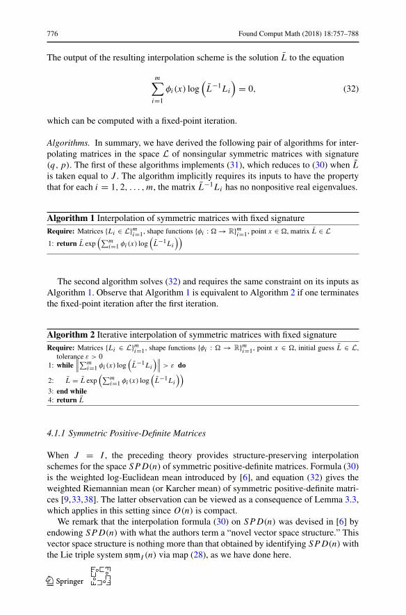
The output of the resulting interpolation scheme is the solution L to the equation
m∑
i=1
φi (x) log(
L−1Li
)
= 0, (32)
which can be computed with a fixed-point iteration.
Algorithms. In summary, we have derived the following pair of algorithms for inter-polating matrices in the space L of nonsingular symmetric matrices with signature(q, p). The first of these algorithms implements (31), which reduces to (30) when Lis taken equal to J . The algorithm implicitly requires its inputs to have the propertythat for each i = 1, 2, . . . ,m, the matrix L−1Li has no nonpositive real eigenvalues.
Algorithm 1 Interpolation of symmetric matrices with fixed signatureRequire: Matrices {Li ∈ L}mi=1, shape functions {φi : → R}mi=1, point x ∈ , matrix L ∈ L1: return L exp
(∑m
i=1 φi (x) log(
L−1Li))
The second algorithm solves (32) and requires the same constraint on its inputs asAlgorithm 1. Observe that Algorithm 1 is equivalent to Algorithm 2 if one terminatesthe fixed-point iteration after the first iteration.
Algorithm 2 Iterative interpolation of symmetric matrices with fixed signatureRequire: Matrices {Li ∈ L}mi=1, shape functions {φi : → R}mi=1, point x ∈ , initial guess L ∈ L,
tolerance ε > 01: while
∥∥∥
∑mi=1 φi (x) log
(
L−1Li)∥∥∥ > ε do
2: L = L exp(∑m
i=1 φi (x) log(
L−1Li))
3: end while4: return L
4.1.1 Symmetric Positive-Definite Matrices
When J = I , the preceding theory provides structure-preserving interpolationschemes for the space SPD(n) of symmetric positive-definite matrices. Formula (30)is the weighted log-Euclidean mean introduced by [6], and equation (32) gives theweighted Riemannian mean (or Karcher mean) of symmetric positive-definite matri-ces [9,33,38]. The latter observation can be viewed as a consequence of Lemma 3.3,which applies in this setting since O(n) is compact.
We remark that the interpolation formula (30) on SPD(n) was devised in [6] byendowing SPD(n) with what the authors term a “novel vector space structure.” Thisvector space structure is nothing more than that obtained by identifying SPD(n) withthe Lie triple system symI (n) via map (28), as we have done here.
123

Found Comput Math (2018) 18:757–788 777
4.1.2 Lorentzian Metrics
When n = 4 and J = diag(−1, 1, 1, 1), the preceding theory provides structure-preserving interpolation schemes for the space of Lorentzian metrics—the space ofsymmetric, nonsingular matrices having signature (3, 1). Lemma 4.1 states that theinterpolation operator (30) in this setting commutes with Lorentz transformations. Bychoosing, for instance, equal to a four-dimensional simplex (or a four-dimensionalhypercube) and {φi }i equal to scalar-valued Lagrange polynomials (or tensor productsof Lagrange polynomials) on , one obtains a family of Lorentzian metric-valuedfinite elements. These elements are capable of interpolating Lorentzian metric-valuedfunctions whose components are continuous on the closure of .
In view of their potential application to numerical relativity, we have numericallycomputed the interpolation error committed by such elements when approximatingthe Schwarzschild metric, which is an explicit solution to Einstein’s equations outsideof a spherical mass [10, p. 193]. In Cartesian coordinates, this metric reads
L(t, x, y, z) =
⎛
⎜⎜⎜⎜⎜⎝
− (1 − Rr
)
0 0 0
0 1 +(
Rr−R
)x2
r2
(R
r−R
)xyr2
(R
r−R
)xzr2
0(
Rr−R
)xyr2
1 +(
Rr−R
)y2
r2
(R
r−R
)yzr2
0(
Rr−R
)xzr2
(R
r−R
)yzr2
1 +(
Rr−R
)z2
r2
⎞
⎟⎟⎟⎟⎟⎠
,
(33)where R (the Schwarzschild radius) is a positive constant (which we take equal to 1in what follows) and r = √
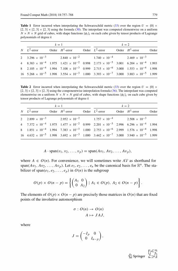
x2 + y2 + z2 > R. We interpolated this metric over theregion U = {0} × [2, 3] × [2, 3] × [2, 3] on a uniform N × N × N grid of cubesusing formula (30) elementwise, with shape functions {φi }i given by tensor productsof Lagrange polynomials of degree k. The results in Table 1 indicate that the L2-error
‖IL − L‖L2(U ) =(∫
U‖IL(t, x, y, z) − L(t, x, y, z)‖2F dx dy dz
)1/2
(34)
(which we approximated with numerical quadrature) converges to zero with order2 and 3, respectively, when using polynomials of degree k = 1 and k = 2. Here,‖ · ‖F denotes the Frobenius norm. In addition, Table 1 indicates that the error in theH1-seminorm (referred to abusively as the H1-error in Table 1)
|IL − L|H1(U ) =⎛
⎝
∫
U
4∑
j=1
∥∥∥∥
∂IL∂ξ j
(t, x, y, z) − ∂L
∂ξ j(t, x, y, z)
∥∥∥∥
2
F
dx dy dz
⎞
⎠
1/2
(35)converges to zero with order 1 and 2, respectively, when using polynomials of degreek = 1 and k = 2. Here, we have denoted ξ = (t, x, y, z).
For the sake of comparison, Table 2 shows the interpolation errors committed whenapplying componentwise polynomial interpolation to the same problem. Within each
123
778 Found Comput Math (2018) 18:757–788
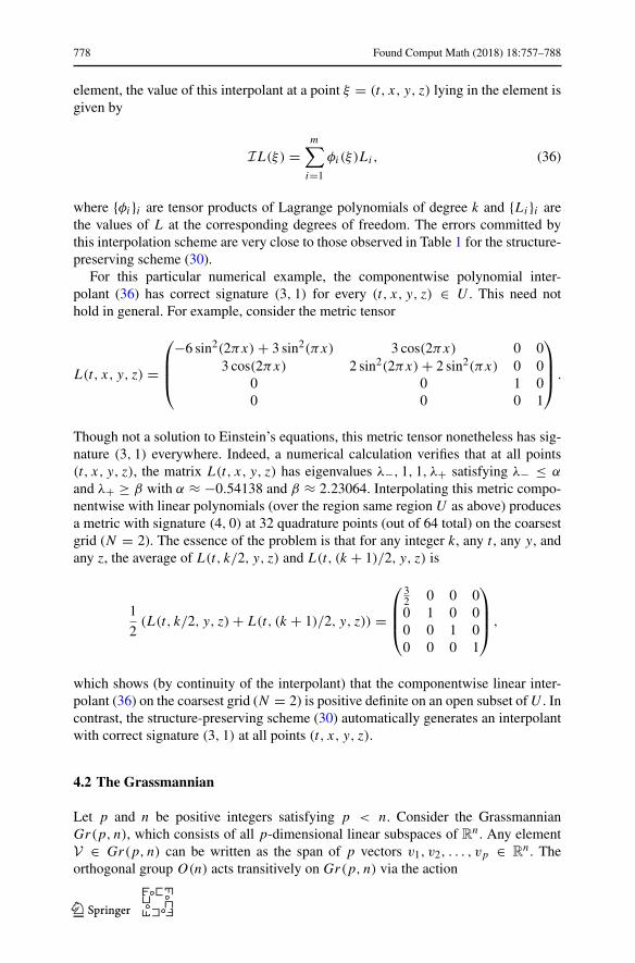
element, the value of this interpolant at a point ξ = (t, x, y, z) lying in the element isgiven by
IL(ξ) =m∑
i=1
φi (ξ)Li , (36)
where {φi }i are tensor products of Lagrange polynomials of degree k and {Li }i arethe values of L at the corresponding degrees of freedom. The errors committed bythis interpolation scheme are very close to those observed in Table 1 for the structure-preserving scheme (30).
For this particular numerical example, the componentwise polynomial inter-polant (36) has correct signature (3, 1) for every (t, x, y, z) ∈ U . This need nothold in general. For example, consider the metric tensor
L(t, x, y, z) =
⎛
⎜⎜⎝
−6 sin2(2πx) + 3 sin2(πx) 3 cos(2πx) 0 03 cos(2πx) 2 sin2(2πx) + 2 sin2(πx) 0 0
0 0 1 00 0 0 1
⎞
⎟⎟⎠
.
Though not a solution to Einstein’s equations, this metric tensor nonetheless has sig-nature (3, 1) everywhere. Indeed, a numerical calculation verifies that at all points(t, x, y, z), the matrix L(t, x, y, z) has eigenvalues λ−, 1, 1, λ+ satisfying λ− ≤ α
and λ+ ≥ β with α ≈ −0.54138 and β ≈ 2.23064. Interpolating this metric compo-nentwise with linear polynomials (over the region same region U as above) producesa metric with signature (4, 0) at 32 quadrature points (out of 64 total) on the coarsestgrid (N = 2). The essence of the problem is that for any integer k, any t , any y, andany z, the average of L(t, k/2, y, z) and L(t, (k + 1)/2, y, z) is
1
2(L(t, k/2, y, z) + L(t, (k + 1)/2, y, z)) =
⎛
⎜⎜⎝
32 0 0 00 1 0 00 0 1 00 0 0 1
⎞
⎟⎟⎠
,
which shows (by continuity of the interpolant) that the componentwise linear inter-polant (36) on the coarsest grid (N = 2) is positive definite on an open subset ofU . Incontrast, the structure-preserving scheme (30) automatically generates an interpolantwith correct signature (3, 1) at all points (t, x, y, z).
4.2 The Grassmannian
Let p and n be positive integers satisfying p < n. Consider the GrassmannianGr(p, n), which consists of all p-dimensional linear subspaces of Rn . Any elementV ∈ Gr(p, n) can be written as the span of p vectors v1, v2, . . . , vp ∈ R
n . Theorthogonal group O(n) acts transitively on Gr(p, n) via the action
123
Found Comput Math (2018) 18:757–788 779
Table 1 Error incurred when interpolating the Schwarzschild metric (33) over the region U = {0} ×[2, 3] × [2, 3] × [2, 3] using the formula (30). The interpolant was computed elementwise on a uniformN × N × N grid of cubes, with shape functions {φi }i on each cube given by tensor products of Lagrangepolynomials of degree k
k = 1 k = 2
N L2-error Order H1-error Order L2-error Order H1-error Order
2 3.296 × 10⁻³ 2.840 × 10⁻² 1.740 × 10⁻⁴ 2.469 × 10⁻³
4 8.383 × 10⁻⁴ 1.975 1.421 × 10⁻² 0.998 2.173 × 10⁻⁵ 3.001 6.204 × 10⁻⁴ 1.993
8 2.105 × 10⁻⁴ 1.994 7.108 × 10⁻³ 0.999 2.715 × 10⁻⁶ 3.000 1.553 × 10⁻⁴ 1.998
16 5.268 × 10⁻⁵ 1.998 3.554 × 10⁻³ 1.000 3.393 × 10⁻⁷ 3.000 3.883 × 10⁻⁵ 1.999
Table 2 Error incurred when interpolating the Schwarzschild metric (33) over the region U = {0} ×[2, 3] × [2, 3] × [2, 3] using the componentwise interpolation formula (36). The interpolant was computedelementwise on a uniform N × N × N grid of cubes, with shape functions {φi }i on each cube given bytensor products of Lagrange polynomials of degree k
k = 1 k = 2
N L2-error Order H1-error Order L2-error Order H1-error Order
2 2.899 × 10⁻³ 2.952 × 10⁻² 1.757 × 10⁻⁴ 2.508 × 10⁻³
4 7.372 × 10⁻⁴ 1.975 1.477 × 10⁻² 0.999 2.201 × 10⁻⁵ 2.996 6.296 × 10⁻⁴ 1.994
8 1.851 × 10⁻⁴ 1.994 7.383 × 10⁻³ 1.000 2.753 × 10⁻⁶ 2.999 1.576 × 10⁻⁴ 1.998
16 4.632 × 10⁻⁵ 1.998 3.692 × 10⁻³ 1.000 3.442 × 10⁻⁷ 3.000 3.940 × 10⁻⁵ 1.999
A · span(v1, v2, . . . , vp) = span(Av1, Av2, . . . , Avp),
where A ∈ O(n). For convenience, we will sometimes write AV as shorthand forspan(Av1, Av2, . . . , Avp). Let e1, e2, . . . , en be the canonical basis for Rn . The sta-bilizer of span(e1, e2, . . . , ep) in O(n) is the subgroup
O(p) × O(n − p) ={(
A1 00 A2
)
| A1 ∈ O(p), A2 ∈ O(n − p)
}
.
The elements of O(p)× O(n − p) are precisely those matrices in O(n) that are fixedpoints of the involutive automorphism
σ : O(n) → O(n)
A �→ J AJ,
where
J =(−Ip 0
0 In−p
)
,
123
780 Found Comput Math (2018) 18:757–788
and Ip and In−p denote the p× p and (n− p)×(n− p) identity matrices, respectively.The matrices in O(n) that are mapped to their inverses by σ constitute the space
SymJ (n) ∩ O(n) = {P ∈ O(n) | P J = J PT }.
The generalized polar decomposition of a matrix A ∈ O(n) in this setting thus reads
A = PQ, P ∈ SymJ (n) ∩ O(n), Q ∈ O(p) × O(n − p). (37)
The corresponding generalized Cartan decomposition reads
Z = X + Y, X ∈ symJ (n) ∩ o(n), Y ∈ o(p) × o(n − p),
where, for each m, o(m) denotes the space of antisymmetric m × m matrices,
o(p) × o(n − p) ={(
Y1 00 Y2
)
| Y1 ∈ o(p), Y2 ∈ o(n − p)
}
,
and
symJ (n) ∩ o(n) = {X ∈ o(n) | X J = J XT }={(
0 −BT
B 0
)
| B ∈ R(n−p)×p
}
.
The map F : symJ (n) ∩ o(n) → Gr(p, n) is given by
F(X) = span(exp(X)e1, exp(X)e2, . . . , exp(X)ep).
The inverse of F can be computed (naively) as follows. Given an element V ∈Gr(p, n), let a1, a2, . . . , ap be an orthonormal basis for V . Extend this basis to anorthonormal basis a1, a2, . . . , an of Rn . Then
F−1(V) = log(P),
where P ∈ SymJ (n) ∩ O(n) is the first factor in the generalized polar decomposi-tion (37) of A = (a1 a2 · · · an). Note that this map is independent of the chosen basesfor V and its orthogonal complement in R
n . Indeed, if a1, a2, . . . , ap is any otherorthonormal basis for V and ap+1, ap+2, . . . , an is any other basis for the orthogonalcomplement of V , then there is a matrix R ∈ O(p) × O(n − p) such that A = AR,where A = (a1 a2 · · · an). The generalized polar decomposition of A is thus A = P Q,where Q = QR.
More generally, we may opt to fix an element A ∈ O(n) and consider interpolantsof the form (17) using the map
FA(X) = span( A exp(X)e1, A exp(X)e2, . . . , A exp(X)ep), (38)
123
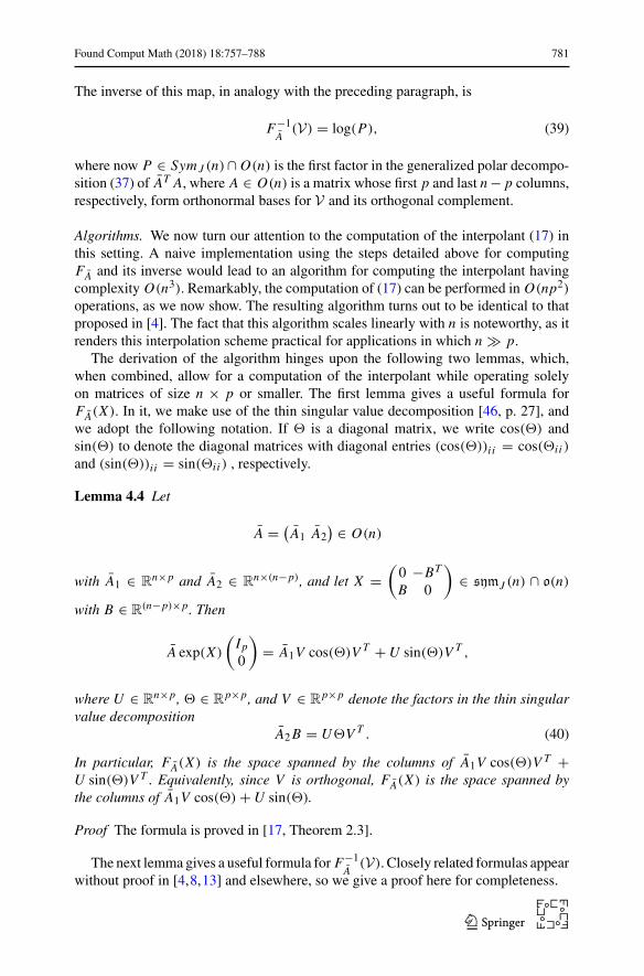
Found Comput Math (2018) 18:757–788 781
The inverse of this map, in analogy with the preceding paragraph, is
F−1A
(V) = log(P), (39)
where now P ∈ SymJ (n)∩ O(n) is the first factor in the generalized polar decompo-sition (37) of AT A, where A ∈ O(n) is a matrix whose first p and last n− p columns,respectively, form orthonormal bases for V and its orthogonal complement.
Algorithms. We now turn our attention to the computation of the interpolant (17) inthis setting. A naive implementation using the steps detailed above for computingFA and its inverse would lead to an algorithm for computing the interpolant havingcomplexity O(n3). Remarkably, the computation of (17) can be performed in O(np2)operations, as we now show. The resulting algorithm turns out to be identical to thatproposed in [4]. The fact that this algorithm scales linearly with n is noteworthy, as itrenders this interpolation scheme practical for applications in which n � p.
The derivation of the algorithm hinges upon the following two lemmas, which,when combined, allow for a computation of the interpolant while operating solelyon matrices of size n × p or smaller. The first lemma gives a useful formula forFA(X). In it, we make use of the thin singular value decomposition [46, p. 27], andwe adopt the following notation. If � is a diagonal matrix, we write cos(�) andsin(�) to denote the diagonal matrices with diagonal entries (cos(�))i i = cos(�i i )
and (sin(�))i i = sin(�i i ) , respectively.
Lemma 4.4 Let
A = (
A1 A2) ∈ O(n)
with A1 ∈ Rn×p and A2 ∈ R
n×(n−p), and let X =(
0 −BT
B 0
)
∈ symJ (n) ∩ o(n)
with B ∈ R(n−p)×p. Then
A exp(X)
(
Ip0
)
= A1V cos(�)V T +U sin(�)V T ,
where U ∈ Rn×p, � ∈ R
p×p, and V ∈ Rp×p denote the factors in the thin singular
value decompositionA2B = U�V T . (40)
In particular, FA(X) is the space spanned by the columns of A1V cos(�)V T +U sin(�)V T . Equivalently, since V is orthogonal, FA(X) is the space spanned bythe columns of A1V cos(�) +U sin(�).
Proof The formula is proved in [17, Theorem 2.3].
The next lemma gives a useful formula for F−1A
(V). Closely related formulas appearwithout proof in [4,8,13] and elsewhere, so we give a proof here for completeness.
123
782 Found Comput Math (2018) 18:757–788
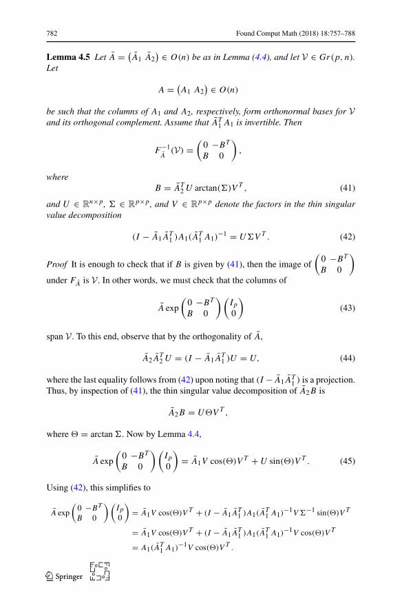
Lemma 4.5 Let A = (
A1 A2) ∈ O(n) be as in Lemma (4.4), and let V ∈ Gr(p, n).
Let
A = (
A1 A2) ∈ O(n)
be such that the columns of A1 and A2, respectively, form orthonormal bases for Vand its orthogonal complement. Assume that AT
1 A1 is invertible. Then
F−1A
(V) =(
0 −BT
B 0
)
,
whereB = AT
2U arctan(�)V T , (41)
and U ∈ Rn×p, � ∈ R
p×p, and V ∈ Rp×p denote the factors in the thin singular
value decomposition
(I − A1 AT1 )A1( A
T1 A1)
−1 = U�V T . (42)
Proof It is enough to check that if B is given by (41), then the image of
(
0 −BT
B 0
)
under FA is V . In other words, we must check that the columns of
A exp
(
0 −BT
B 0
)(
Ip0
)
(43)
span V . To this end, observe that by the orthogonality of A,
A2 AT2U = (I − A1 A
T1 )U = U, (44)
where the last equality follows from (42) upon noting that (I − A1 AT1 ) is a projection.
Thus, by inspection of (41), the thin singular value decomposition of A2B is
A2B = U�V T ,
where � = arctan�. Now by Lemma 4.4,
A exp
(
0 −BT
B 0
)(
Ip0
)
= A1V cos(�)V T +U sin(�)V T . (45)
Using (42), this simplifies to
A exp
(
0 −BT
B 0
)(
Ip0
)
= A1V cos(�)V T + (I − A1 AT1 )A1( A
T1 A1)
−1V�−1 sin(�)V T
= A1V cos(�)V T + (I − A1 AT1 )A1( A
T1 A1)
−1V cos(�)V T
= A1( AT1 A1)
−1V cos(�)V T .
123
Found Comput Math (2018) 18:757–788 783
Observe that since � = tan(�) is finite, the diagonal entries of cos(�) are nonzero.Thus, ( AT
1 A1)−1V cos(�)V T is invertible, so we conclude that the columns of (43)
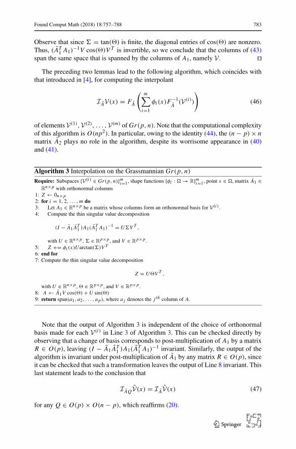
span the same space that is spanned by the columns of A1, namely V . The preceding two lemmas lead to the following algorithm, which coincides with
that introduced in [4], for computing the interpolant
I AV(x) = FA
(m∑
i=1
φi (x)F−1A
(V(i))
)
(46)
of elements V(1),V(2), . . . ,V(m) ofGr(p, n). Note that the computational complexityof this algorithm is O(np2). In particular, owing to the identity (44), the (n − p) × nmatrix A2 plays no role in the algorithm, despite its worrisome appearance in (40)and (41).
Algorithm 3 Interpolation on the Grassmannian Gr(p, n)
Require: Subspaces {V(i) ∈ Gr(p, n)}mi=1, shape functions {φi : → R}mi=1, point x ∈ , matrix A1 ∈Rn×p with orthonormal columns
1: Z ← 0n×p2: for i = 1, 2, . . . ,m do3: Let A1 ∈ R
n×p be a matrix whose columns form an orthonormal basis for V(i).4: Compute the thin singular value decomposition
(I − A1 AT1 )A1( A
T1 A1)
−1 = U�V T ,
with U ∈ Rn×p , � ∈ R
p×p , and V ∈ Rp×p .
5: Z += φi (x)Uarctan(�)V T
6: end for7: Compute the thin singular value decomposition
Z = U�V T ,
with U ∈ Rn×p , � ∈ R
p×p , and V ∈ Rp×p .
8: A ← A1V cos(�) +U sin(�)
9: return span(a1, a2, . . . , ap), where a j denotes the j th column of A.
Note that the output of Algorithm 3 is independent of the choice of orthonormalbasis made for each V(i) in Line 3 of Algorithm 3. This can be checked directly byobserving that a change of basis corresponds to post-multiplication of A1 by a matrixR ∈ O(p), leaving (I − A1 AT
1 )A1( AT1 A1)
−1 invariant. Similarly, the output of thealgorithm is invariant under post-multiplication of A1 by any matrix R ∈ O(p), sinceit can be checked that such a transformation leaves the output of Line 8 invariant. Thislast statement leads to the conclusion that
I AQV(x) = I AV(x) (47)
for any Q ∈ O(p) × O(n − p), which reaffirms (20).
123
784 Found Comput Math (2018) 18:757–788
The interpolant so constructed enjoys the following additional property.
Lemma 4.6 The interpolant (46) commutes with the action of O(n) on Gr(p, n).That is, if Q ∈ O(n) and V(i) = QV(i), i = 1, 2, . . . ,m, then
IQAV(x) = QI AV(x)
for every x ∈ .
Proof Apply (18). Another O(n)-equivariant interpolant on Gr(p, n) is given abstractly by (22). In
this setting, this interpolant is obtained by solving
m∑
i=1
φi (x)F−1A
(V(i)) = 0
for A and outputting the space spanned by the first p columns of A. Algorithmically,this amounts towrapping a fixed-point iteration aroundAlgorithm 3, as detailed below.
Algorithm 4 Iterative interpolation on the Grassmannian Gr(p, n)
Require: Subspaces {V(i) ∈ Gr(p, n)}mi=1, shape functions {φi : → R}mi=1, point x ∈ , matrix A1 ∈Rn×p with orthonormal columns
1: repeat2: Use Algorithm 3 to compute the interpolant of {V(i)}mi=1 at x , storing the result as a matrix
A ∈ Rn×p (i.e., the matrix A appearing in line 8 of Algorithm 3).
3: A1 ← A4: until converged5: return span(a1, a2, . . . , ap), where a j denotes the j th column of A1.
Since O(p) × O(n − p) is compact, Lemma 3.3 shows that Algorithm 4 producesthe weighted Riemannian mean on Gr(p, n). This interpolant has been consideredpreviously by several authors, including [8,13,21].
4.3 Lie Groups
It was remarked in Sect. 2.2 that any Lie group G can be realized as a symmetricspace (G × G)/diag(G × G), since diag(G × G) = {(g, g) | g ∈ G} fulfills tworoles simultaneously: it is the stabilizer of e ∈ G under the action of G × G on Ggiven by (g, h) · k = gkh−1, and it is the subgroup (G × G)σ of fixed points of theinvolutive automorphism σ(g, h) = (h, g). In the notation of Sect. 2, one checks that(G × G)σ = {(g, h) | g = h−1}, p = {(X,−X) | X ∈ g}, k = {(X, X) | X ∈ g},and F(X,−X) = exp(2X). Thus, the interpolant (11) of a collection of elements
123
Found Comput Math (2018) 18:757–788 785
g1, g2, . . . , gm ∈ G reads
Ig(x) = exp
(m∑
i=1
φi (x) log(gi )
)
.
This is of course a standard strategy for interpolation on Lie groups that enjoyswidespread use [39], and it belongs to a broad class of methods that perform interpola-tion on Lie groups by mapping elements of G to g and back [36,45]. This interpolant,being (G ×G)σ -equivariant, commutes with the adjoint action of G on itself. That is,I(hgh)−1(x) = hIg(x)h−1 for every h ∈ G sufficiently close to the identity e ∈ G.However, it is not G-equivariant (I(hg)(x) �= hIg(x) in general), and it has the dis-advantage of requiring that each gi be close to e. The variant (21) overcomes theselimitations by seeking a solution g ∈ G to the equation
g = exp
(m∑
i=1
φi (x) log(g−1gi )
)
,
which defines a geodesic finite element [22,43,44] ifG is equipped with a bi-invariantmetric (so that the Lie group exponential and Riemannian exponential maps coincide).The latter interpolant exists whenever g1, g2, . . . , gm are sufficiently close to oneanother [22, Theorem 3.1], and it is manifestly G-equivariant.
5 Conclusion
This paper has presented a family of structure-preserving interpolation operators forfunctions taking values in a symmetric space S. We accomplished this by identifyingS with a homogeneous space G/Gσ and interpolating coset representatives obtainedfrom the generalized polar decomposition. The resulting interpolation operators enjoyequivariance with respect to the action of Gσ on S, equivariance with respect to theaction of certain geodesic symmetries on S, and optimal approximation properties.The application of these interpolation schemes seems intriguing, particularly in thecontext of numerical relativity, where they provide structure-preserving finite elementsfor the metric tensor.
Acknowledgements EG has been supported in part by NSF under Grants DMS-1411792, DMS-1345013.ML has been supported in part by NSF under Grants DMS-1010687, CMMI-1029445, DMS-1065972,CMMI-1334759, DMS-1411792, DMS-1345013.
Appendix A: Second-Order Derivatives of the Matrix Exponential
In this section, we prove (16) by showing that if IP : → Rn×n is a smooth matrix-
valued function defined on a domain ⊂ Rd , then, for each j, k = 1, 2, . . . , d, the
matrix ∂2
∂x j ∂xkexp(IP(x)) is given by reading off the (1, 4) block of
123
786 Found Comput Math (2018) 18:757–788
exp
⎛
⎜⎜⎝
X Y Z W0 X 0 Z0 0 X Y0 0 0 X
⎞
⎟⎟⎠
, (48)
where X = IP(x), Y = ∂IP∂x j
(x), Z = ∂IP∂xk
(x), and W = ∂2IP∂x j ∂xk
(x). To prove this,recall first the identity (15), which can be written as
d
dt
∣∣∣∣t=0
exp(U + tV ) = R[
exp
(
U V0 U
)]
(49)
for any square matricesU and V of equal size, whereR denotes the map which sendsa 2l × 2l matrix B to the l × l submatrix of B consisting of the intersection of thefirst l rows and last l columns of B. Now observe that with X , Y , Z , and W definedas above,
∂2
∂x j∂xkexp(IP(x)) = ∂2
∂s ∂t
∣∣∣∣s=t=0
exp(X + tY + sZ + stW )
= ∂
∂s
∣∣∣∣s=0
∂
∂t
∣∣∣∣t=0
exp(X + sZ + t (Y + sW ))
= ∂
∂s
∣∣∣∣s=0
R[
exp
(
X + sZ Y + sW0 X + sZ
)]
= R[
∂
∂s
∣∣∣∣s=0
exp
(
X + sZ Y + sW0 X + sZ
)]
Using (49) again, we have
∂
∂s
∣∣∣∣s=0
exp
(
X + sZ Y + sW0 X + sZ
)
= R
⎡
⎢⎢⎣exp
⎛
⎜⎜⎝
X Y Z W0 X 0 Z0 0 X Y0 0 0 X
⎞
⎟⎟⎠
⎤
⎥⎥⎦
.
This shows that
∂2
∂x j∂xkexp(IP(x)) = R
⎡
⎢⎢⎣R
⎡
⎢⎢⎣exp
⎛
⎜⎜⎝
X Y Z W0 X 0 Z0 0 X Y0 0 0 X
⎞
⎟⎟⎠
⎤
⎥⎥⎦
⎤
⎥⎥⎦
,
which is precisely the (1, 4) block of matrix (48).
123
Found Comput Math (2018) 18:757–788 787
References
1. P.-A. Absil, R. Mahony, and R. Sepulchre. Optimization Algorithms on Matrix Mani- folds. PrincetonUniversity Press, 2009.
2. P.-A. Absil, R. Mahony, and R. Sepulchre. Riemannian geometry of Grassmann manifolds with a viewon algorithmic computation. Acta Applicandae Mathematica 80.2 (2004), pp. 199–220.
3. A. H. Al-Mohy and N. J. Higham. Computing the Fréchet derivative of the matrix exponential, with anapplication to condition number estimation. SIAM Journal on Matrix Analysis and Applications 30.4(2009), pp. 1639–1657
4. D. Amsallem and C. Farhat. Interpolation method for adapting reduced-order models and applicationto aeroelasticity. AIAA Journal 46.7 (2008), pp. 1803–1813.
5. D. N. Arnold. Numerical problems in general relativity. Numerical Mathematics and Advanced Appli-cations (P. Neittaanmki, T. Tiihonen, and P. Tarvainen, eds.), World Scientific (2000), pp. 3–15.
6. V. Arsigny, P. Fillard, X. Pennec, and N. Ayache. Geometric means in a novel vector space structure onsymmetric positive-definite matrices. SIAM Journal onMatrix Analysis and Applications 29.1 (2007),pp. 328–347.
7. V. Arsigny, P. Fillard, X. Pennec, and N. Ayache. Log-Euclidean metrics for fast and simple calculuson diffusion tensors. Magnetic Resonance in Medicine 56.2 (2006), pp. 411–421.
8. E. Begelfor and M. Werman. Affine invariance revisited. Conference on Computer Vision and PatternRecognition. IEEE. 2006, pp. 2087–2094.
9. R. Bhatia. The Riemannian mean of positive matrices. Matrix Information Geometry. Springer, 2013,pp. 35–51.
10. S. M. Carroll. Spacetime and Geometry: An Introduction to General Relativity. San Francisco, CA,USA: Addison Wesley, 2004.
11. E. Celledoni, M. Eslitzbichler, and A. Schmeding. Shape Analysis on Lie Groups with Applicationsin Computer Animation. arXiv preprint arXiv:1506.00783 (2015).
12. E. Celledoni and A. Iserles. Approximating the exponential from a Lie algebra to a Lie group. Math.Comp. 69.232 (2000), pp. 1457–1480.
13. J.-M. Chang, C. Peterson, M. Kirby, et al. Feature patch illumination spaces and Karcher compressionfor face recognition via Grassmannians. Advances in Pure Mathematics 2.04 (2012), p. 226.
14. F Demoures et al. Discrete variational Lie group formulation of geometrically exact beam dynamics.Numerische Mathematik 130.1 (2015), pp. 73-123.
15. I. L. Dryden and K. V. Mardia. Statistical Shape Analysis: With Applications in R. Wiley, 2016.16. T. Duchamp, G. Xie, and T. P.-Y. Yu. Single basepoint subdivision schemes for manifold-valued data:
time-symmetry without space-symmetry. Foundations of Com- putational Mathematics 13.5 (2013),pp. 693–728. doi:10.1007/s10208-013-9144-1.
17. A. Edelman, T. A. Arias, and S. T. Smith. The geometry of algorithms with orthogonality constraints.SIAM Journal on Matrix Analysis and Applications 20.2 (1998), pp. 303–353.
18. P. T. Fletcher, C. Lu, and S. Joshi. Statistics of shape via principal geodesic analysis on Lie groups.2003 IEEE Computer Society Conference on Computer Vision and Pattern Recognition. Vol. 1. IEEE.2003, pp. 1–7.
19. K. A. Gallivan, A. Srivastava, X. Liu, and P. Van Dooren. Efficient algorithms for inferences ongrassmann manifolds. 2003 IEEE Workshop on Statistical Signal Processing. IEEE. 2003, pp. 315–318.
20. F. de Goes, B. Liu, M. Budninskiy, Y. Tong, and M. Desbrun. Discrete 2-Tensor Fields on Triangula-tions. Computer Graphics Forum. Vol. 33. 5.Wiley Online Library. 2014, pp. 13–24.
21. P. Grohs. Quasi-interpolation in Riemannian manifolds. IMA Journal of Numerical Analysis 33.3(2013), pp. 849–874.
22. P. Grohs, H. Hardering, and O. Sander. Optimal a priori discretization error bounds for geodesic finiteelements. Foundations of Computational Mathematics 15.6 (2015), pp. 1357–1411.
23. P. Grohs, M. Sprecher, and T. Yu. Scattered manifold-valued data approximation. Numerische Math-ematik 135.4 (2017), pp. 987–1010. doi:10.1007/s00211-016-0823-0.
24. J. Hall and M. Leok. Lie group spectral variational integrators. Foundations of Computational Mathe-matics, pp. 1–59.
25. S. Helgason. Differential Geometry, Lie Groups, and Symmetric Spaces. Vol. 80. Academic press,1979.
26. N. J. Higham. Functions of Matrices: Theory and Computation. SIAM, 2008.
123
788 Found Comput Math (2018) 18:757–788
27. N. J. Higham. J-orthogonal matrices: Properties and generation. SIAM review 45.3 (2003), pp. 504–519.
28. N. J. Higham, C. Mehl, and F. Tisseur. The canonical generalized polar decomposition. SIAM Journalon Matrix Analysis and Applications 31.4 (2010), pp. 2163–2180.
29. J. Hilgert and K.-H. Neeb. Structure and Geometry of Lie Groups. Springer, 2011.30. Y. Hong et al. Geodesic regression on the Grassmannian. Computer Vision-ECCV 2014. Springer,
2014, pp. 632–646.31. A. Iserles and A. Zanna. Efficient computation of the matrix exponential by generalized polar decom-
positions. SIAM Journal on Numerical Analysis 42.5 (2005), pp. 2218–2256.32. T. Jiang et al. Frame field generation through metric customization. ACM Transactions on Graphics
(TOG) 34.4 (2015), p. 40.33. H. Karcher. Riemannian center ofmass andmollifier smoothing. Communications on Pure andApplied
Mathematics 30.5 (1977), pp. 509–541.34. A. W. Knapp. Lie Groups: Beyond an Introduction. Vol. 140. Springer, 2013.35. S. Kobayashi and K. Nomizu. Foundations of Differential Geometry. Vol. 2.Wiley New York, 1969.36. A. Marthinsen. Interpolation in Lie groups. SIAM Journal on Numerical Analysis 37.1 (1999), pp.
269–285.37. R. Mathias. A chain rule for matrix functions and applications. SIAM Journal on Matrix Analysis and
Applications 17.3 (1996), pp. 610–620.38. M. Moakher. A differential geometric approach to the geometric mean of symmetric positive-definite
matrices. SIAM Journal on Matrix Analysis and Applications 26.3 (2005), pp. 735–747.39. A. Mota, W. Sun, J. T. Ostien, J. W. Foulk, and K. N. Long. Lie-group interpolation and variational
recovery for internal variables. Computational Mechanics 52.6 (2013), pp. 1281–1299.40. H. Z. Munthe-Kaas, G. R.W. Quispel, and A. Zanna. Symmetric spaces and Lie triple systems in
numerical analysis of differential equations. BIT Numerical Mathematics 54.1 (2014), pp. 257–282.41. H. Z. Munthe-Kaas, G. Quispel, and A. Zanna. Generalized polar decompositions on Lie groups with
involutive automorphisms. Foundations of Computational Mathematics 1.3 (2001), pp. 297–324.42. O. Sander. Geodesic finite elements for Cosserat rods. International Journal for Numerical Methods in
Engineering 82.13 (2010), pp. 1645–1670.43. O. Sander. Geodesic finite elements of higher order. IMA J. Numer. Anal. 36.1 (2016), pp. 238–266.44. O. Sander. Geodesic finite elements on simplicial grids. International Journal for Numerical Methods
in Engineering 92.12 (2012), pp. 999–1025.45. T. Shingel. Interpolation in special orthogonal groups. IMA Journal of Numerical Analysis (2008).46. L. N. Trefethen and D. Bau III. Numerical Linear Algebra. Vol. 50. SIAM, 1997.47. P. Turaga, A. Veeraraghavan, A. Srivastava, and R. Chellappa. Statistical computations on Grassmann
and Stiefel manifolds for image and video-based recognition. IEEE Transactions on Pattern Analysisand Machine Intelligence 33.11 (2011), pp. 2273–2286.
48. F. Vetrano, C. Le Garrec, G. D. Mortchelewicz, and R. Ohayon. Assessment of strategies for interpo-lating POD based reduced order models and application to aeroelasticity. Journal of Aeroelasticity andStructural Dynamics 2.2 (2012).
49. J. Wallner, E. N. Yazdani, and A. Weinmann. Convergence and smoothness analysis of subdivisionrules in Riemannian and symmetric spaces. Advances in Computational Mathematics 34.2 (2011), pp.201–218.
50. E. N. Yazdani and T. P.-Y. Yu. On Donoho’s Log-Exp subdivision scheme: choice of retraction andtime-symmetry. Multiscale Modeling and Simulation 9.4 (2011), pp. 1801–1828.
123
![GENERALIZED FROBENIUS ALGEBRAS AND HOPF ALGEBRAS · 2013-11-26 · GENERALIZED FROBENIUS ALGEBRAS AND HOPF ALGEBRAS 3 techniques of [I] can be extended and applied to obtain a symmetric](https://img.pdfslide.us/doc/110x75/5edc9faaad6a402d66675e9e/generalized-frobenius-algebras-and-hopf-algebras-2013-11-26-generalized-frobenius.jpg)