Embed Size (px)
Citation preview
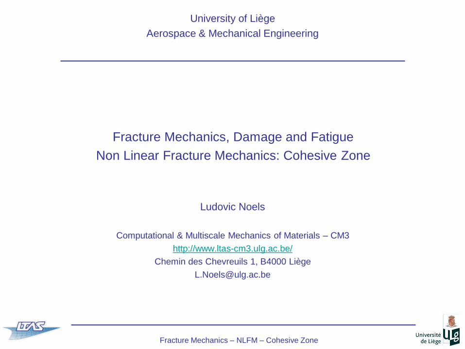
University of Liège
Aerospace & Mechanical Engineering
Fracture Mechanics, Damage and Fatigue
Non Linear Fracture Mechanics: Cohesive Zone
Ludovic Noels
Computational & Multiscale Mechanics of Materials – CM3
http://www.ltas-cm3.ulg.ac.be/
Chemin des Chevreuils 1, B4000 Liège
Fracture Mechanics – NLFM – Cohesive Zone
Elastic fracture
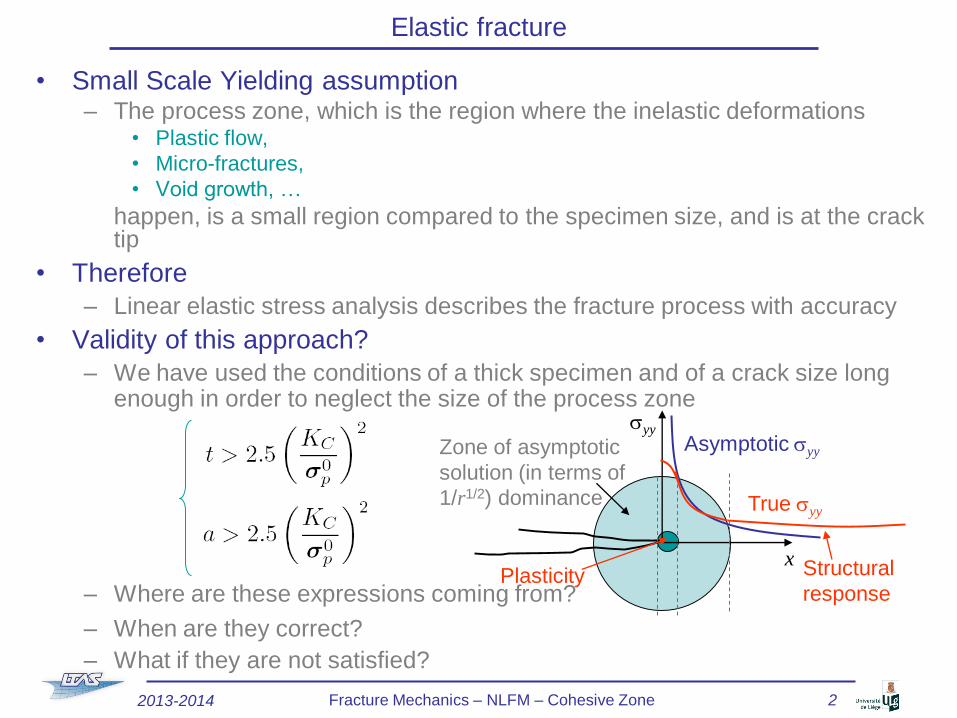
• Small Scale Yielding assumption– The process zone, which is the region where the inelastic deformations
• Plastic flow,
• Micro-fractures,
• Void growth, …
happen, is a small region compared to the specimen size, and is at the crack tip
• Therefore
– Linear elastic stress analysis describes the fracture process with accuracy
• Validity of this approach?
– We have used the conditions of a thick specimen and of a crack size long enough in order to neglect the size of the process zone
– Where are these expressions coming from?
– When are they correct?
– What if they are not satisfied?
syy
x
Asymptotic syy
True syy
Zone of asymptotic
solution (in terms of
1/r1/2) dominance
Structural
responsePlasticity
2013-2014 Fracture Mechanics – NLFM – Cohesive Zone 2
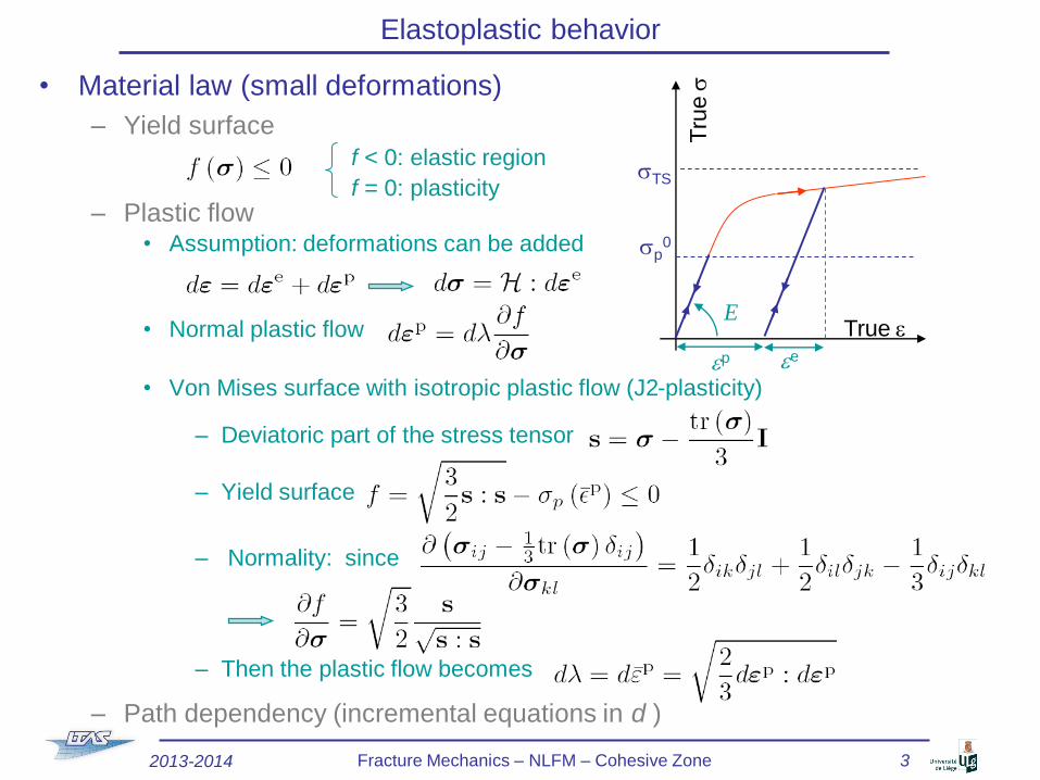
• Material law (small deformations)
– Yield surface
f < 0: elastic region
f = 0: plasticity– Plastic flow
• Assumption: deformations can be added
• Normal plastic flow
• Von Mises surface with isotropic plastic flow (J2-plasticity)
– Deviatoric part of the stress tensor
– Yield surface
– Normality: since
– Then the plastic flow becomes
– Path dependency (incremental equations in d )
Elastoplastic behavior
True e
Tru
es
sTS
sp0
ep ee
E
2013-2014 Fracture Mechanics – NLFM – Cohesive Zone 3
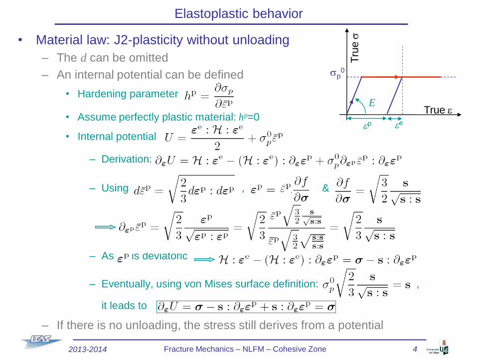
• Material law: J2-plasticity without unloading
– The d can be omitted
– An internal potential can be defined
• Hardening parameter
• Assume perfectly plastic material: hp=0
• Internal potential
– Derivation:
– Using , &
– As is deviatoric
– Eventually, using von Mises surface definition: ,
it leads to
– If there is no unloading, the stress still derives from a potential
Elastoplastic behavior
True e
Tru
es
sp0
ep ee
E
2013-2014 Fracture Mechanics – NLFM – Cohesive Zone 4
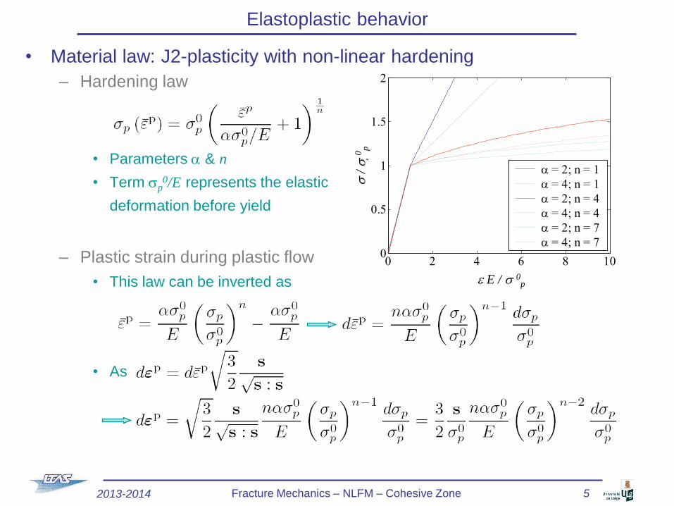
• Material law: J2-plasticity with non-linear hardening
– Hardening law
• Parameters a & n
• Term sp0/E represents the elastic
deformation before yield
– Plastic strain during plastic flow
• This law can be inverted as
• As
Elastoplastic behavior
2013-2014 Fracture Mechanics – NLFM – Cohesive Zone 5
0 2 4 6 8 100
0.5
1
1.5
2
e E/sp
0
s/ s
p0
a = 2; n = 1
a = 4; n = 1
a = 2; n = 4
a = 4; n = 4
a = 2; n = 7
a = 4; n = 7
s/
s 0
p
e E / s 0p
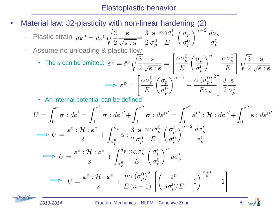
• Material law: J2-plasticity with non-linear hardening (2)
– Plastic strain
– Assume no unloading & plastic flow
• The d can be omitted:
• An internal potential can be defined
Elastoplastic behavior
2013-2014 Fracture Mechanics – NLFM – Cohesive Zone 6
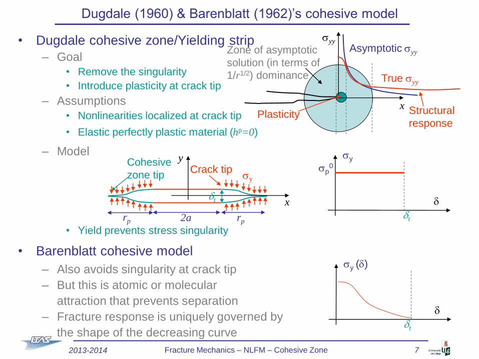
Dugdale (1960) & Barenblatt (1962)’s cohesive model
• Dugdale cohesive zone/Yielding strip
– Goal
• Remove the singularity
• Introduce plasticity at crack tip
– Assumptions
• Nonlinearities localized at crack tip
• Elastic perfectly plastic material (hp=0)
– Model
• Yield prevents stress singularity
• Barenblatt cohesive model
– Also avoids singularity at crack tip
– But this is atomic or molecular
attraction that prevents separation
– Fracture response is uniquely governed by
the shape of the decreasing curve
syy
x
Asymptotic syy
True syy
Zone of asymptotic
solution (in terms of
1/r1/2) dominance
Structural
responsePlasticity
2a rprp
Crack tipCohesive
zone tip
x
y
sy
dt d
sy
sp0
dt
d
sy (d)
dt
2013-2014 Fracture Mechanics – NLFM – Cohesive Zone 7
Dugdale (1960) & Barenblatt (1962)’s cohesive model
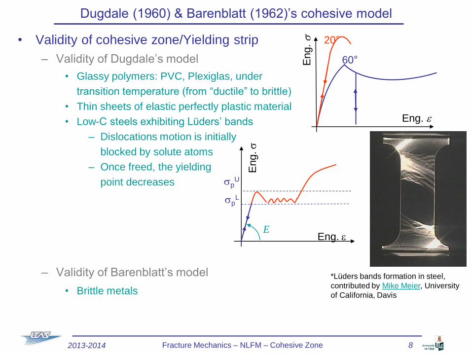
• Validity of cohesive zone/Yielding strip
– Validity of Dugdale’s model
• Glassy polymers: PVC, Plexiglas, under
transition temperature (from “ductile” to brittle)
• Thin sheets of elastic perfectly plastic material
• Low-C steels exhibiting Lüders’ bands
– Dislocations motion is initially
blocked by solute atoms
– Once freed, the yielding
point decreases
– Validity of Barenblatt’s model
• Brittle metals
Eng. e
Eng.
s
spU
spL
E
*Lüders bands formation in steel,
contributed by Mike Meier, University
of California, Davis
Eng.
s
Eng. e
20°
60°
2013-2014 Fracture Mechanics – NLFM – Cohesive Zone 8
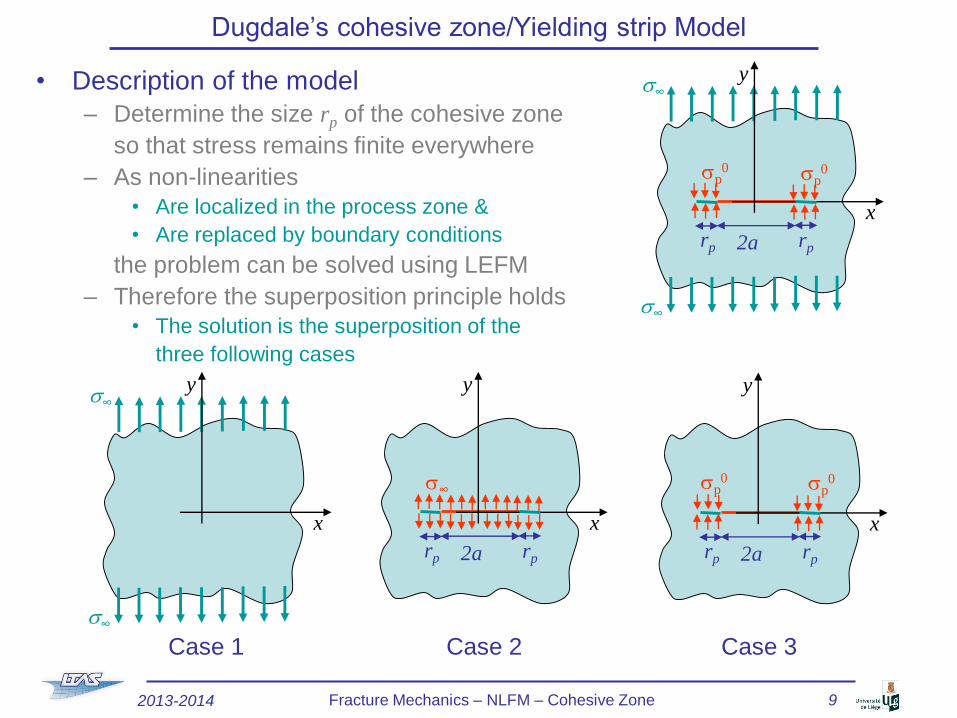
Dugdale’s cohesive zone/Yielding strip Model
• Description of the model
– Determine the size rp of the cohesive zone
so that stress remains finite everywhere
– As non-linearities
• Are localized in the process zone &
• Are replaced by boundary conditions
the problem can be solved using LEFM
– Therefore the superposition principle holds
• The solution is the superposition of the
three following cases
2a
x
ys∞
s∞
rprp
sp0sp
0
x
ys∞
s∞
Case 1 Case 2 Case 3
2a
x
y
rprp
s∞
2a
x
y
rprp
sp0 sp
0
2013-2014 Fracture Mechanics – NLFM – Cohesive Zone 9
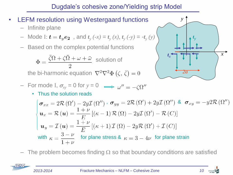
Dugdale’s cohesive zone/Yielding strip Model
• LEFM resolution using Westergaard functions
– Infinite plane
– Mode I: , and ty (-x) = ty (x), ty (-y) = -ty (y)
– Based on the complex potential functions
solution of
the bi-harmonic equation
– For mode I, sxy = 0 for y = 0
• Thus the solution reads
, &
with for plane stress & for plane strain
– The problem becomes finding W so that boundary conditions are satisfied
2a
x
y
ty
tx
2013-2014 Fracture Mechanics – NLFM – Cohesive Zone 10
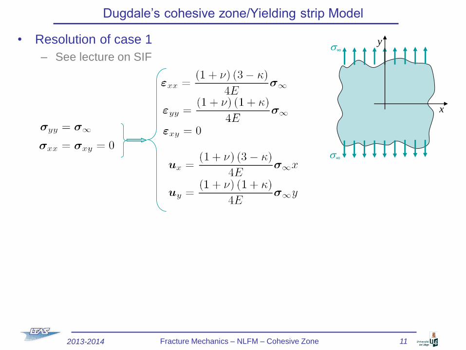
Dugdale’s cohesive zone/Yielding strip Model
• Resolution of case 1
– See lecture on SIF
x
ys∞
s∞
2013-2014 Fracture Mechanics – NLFM – Cohesive Zone 11
2a
x
y
rprp
s∞
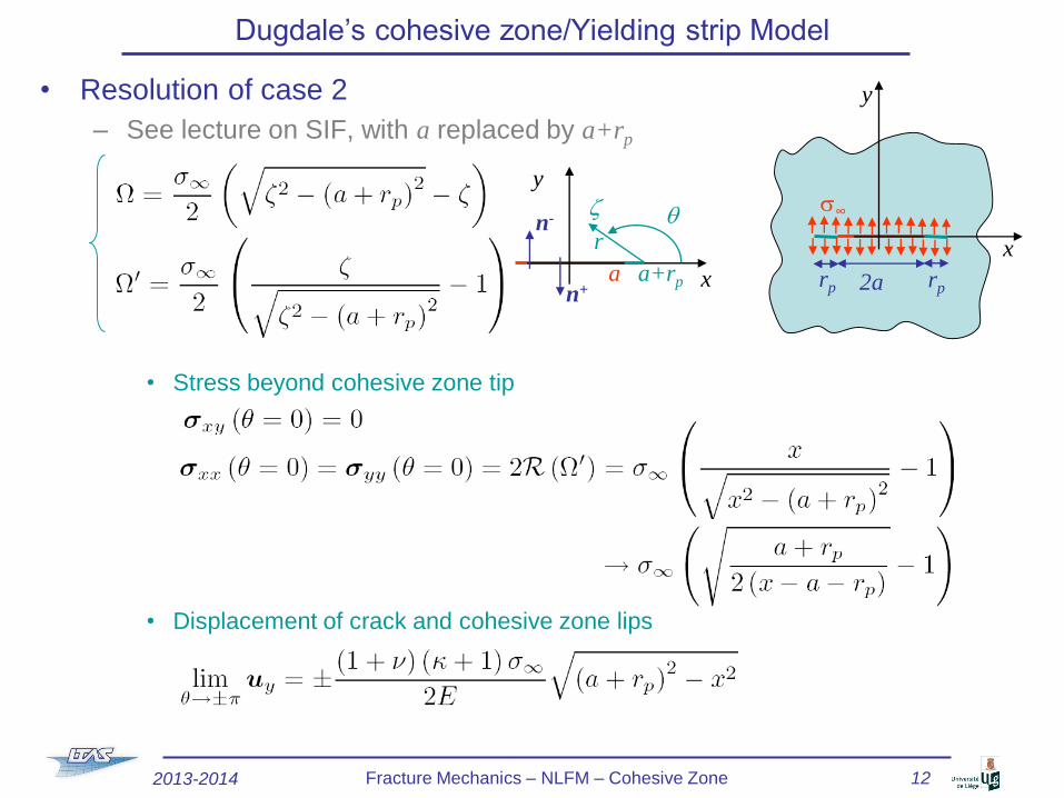
Dugdale’s cohesive zone/Yielding strip Model
• Resolution of case 2
– See lecture on SIF, with a replaced by a+rp
• Stress beyond cohesive zone tip
• Displacement of crack and cohesive zone lips
a a+rp
y
x
qr
z
n+
n-
2013-2014 Fracture Mechanics – NLFM – Cohesive Zone 12
2a
x
y
rprp
sp0 sp
0
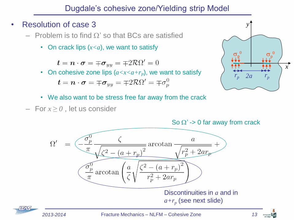
Dugdale’s cohesive zone/Yielding strip Model
• Resolution of case 3
– Problem is to find W’ so that BCs are satisfied
• On crack lips (x<a), we want to satisfy
• On cohesive zone lips (a<x<a+rP), we want to satisfy
• We also want to be stress free far away from the crack
– For x ≥ 0 , let us consider
Discontinuities in a and in
a+rp (see next slide)
So W’ -> 0 far away from crack
2013-2014 Fracture Mechanics – NLFM – Cohesive Zone 13
2a
x
y
rprp
sp0 sp
0
Dugdale’s cohesive zone/Yielding strip Model
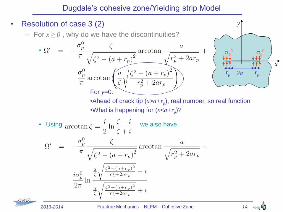
• Resolution of case 3 (2)
– For x ≥ 0 , why do we have the discontinuities?
•
• Using we also have
For y=0:
•Ahead of crack tip (x>a+rp), real number, so real function
•What is happening for (x<a+rp)?
2013-2014 Fracture Mechanics – NLFM – Cohesive Zone 14
2a
x
y
rprp
sp0 sp
0
Dugdale’s cohesive zone/Yielding strip Model
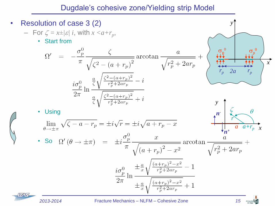
• Resolution of case 3 (2)
– For z = x±|e| i, with x <a+rp,
• Start from
• Using
• So
a a+rp
y
x
qr
z
n+
n-
2013-2014 Fracture Mechanics – NLFM – Cohesive Zone 15
Dugdale’s cohesive zone/Yielding strip Model
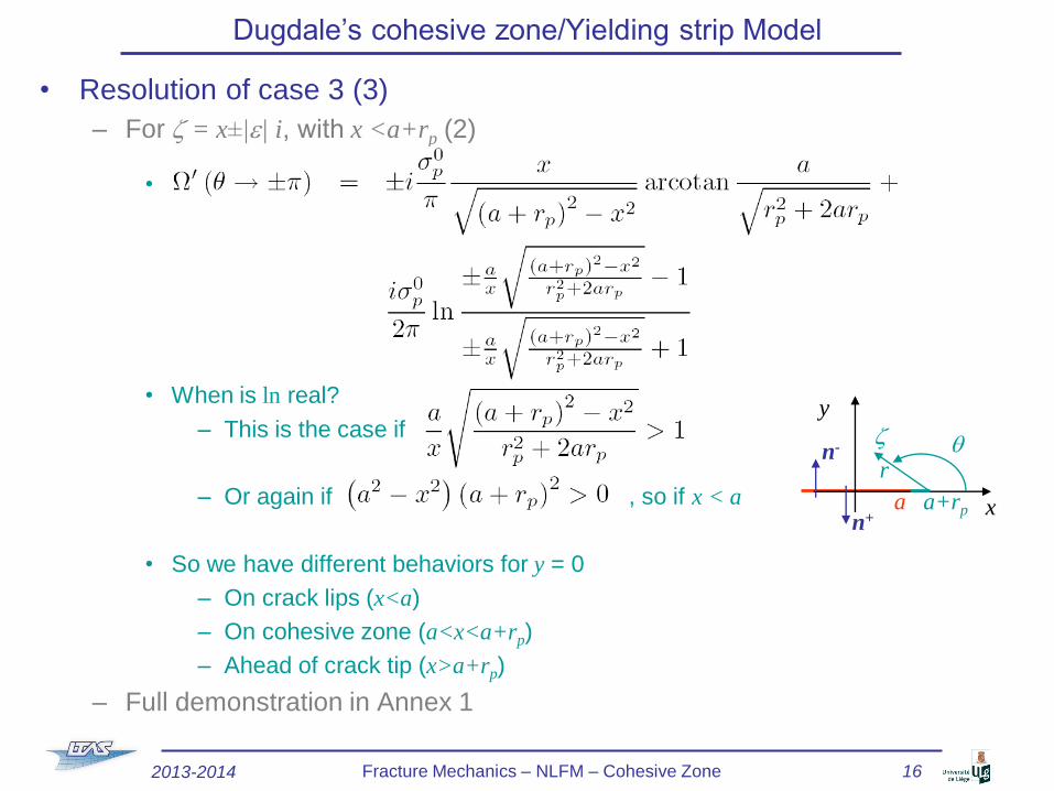
• Resolution of case 3 (3)
– For z = x±|e| i, with x <a+rp (2)
•
• When is ln real?
– This is the case if
– Or again if , so if x < a
• So we have different behaviors for y = 0
– On crack lips (x<a)
– On cohesive zone (a<x<a+rp)
– Ahead of crack tip (x>a+rp)
– Full demonstration in Annex 1
a a+rp
y
x
qr
z
n+
n-
2013-2014 Fracture Mechanics – NLFM – Cohesive Zone 16
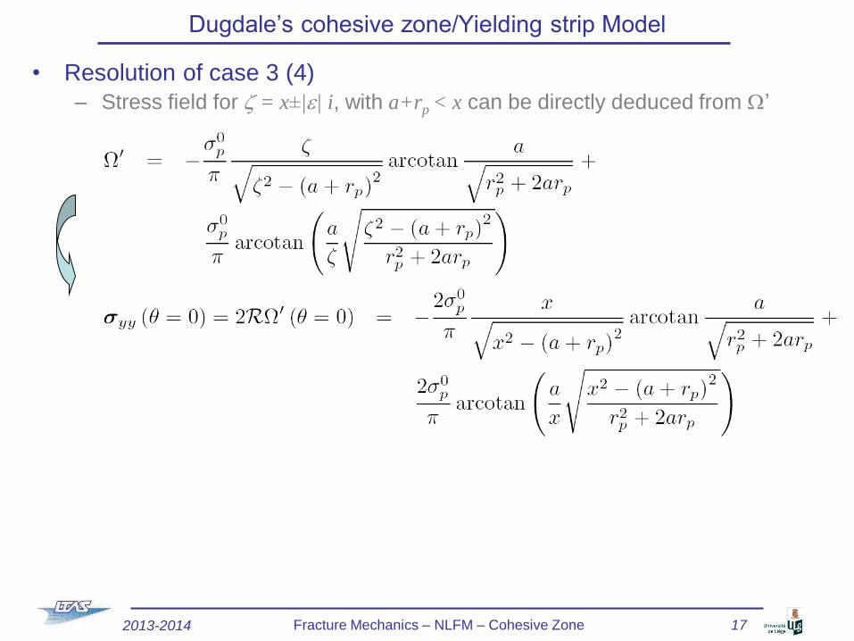
• Resolution of case 3 (4)
– Stress field for z = x±|e| i, with a+rp < x can be directly deduced from W’
Dugdale’s cohesive zone/Yielding strip Model
2013-2014 Fracture Mechanics – NLFM – Cohesive Zone 17
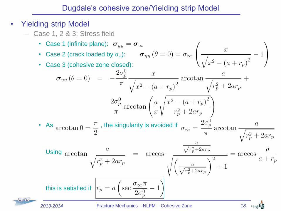
• Yielding strip Model
– Case 1, 2 & 3: Stress field
• Case 1 (infinite plane):
• Case 2 (crack loaded by s∞):
• Case 3 (cohesive zone closed):
• As , the singularity is avoided if
Using
this is satisfied if
Dugdale’s cohesive zone/Yielding strip Model
2013-2014 Fracture Mechanics – NLFM – Cohesive Zone 18
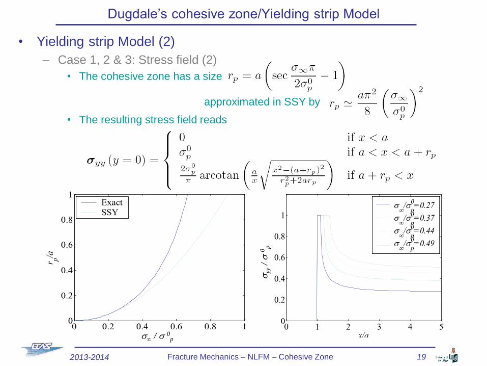
• Yielding strip Model (2)
– Case 1, 2 & 3: Stress field (2)
• The cohesive zone has a size
approximated in SSY by
• The resulting stress field reads
Dugdale’s cohesive zone/Yielding strip Model
2013-2014 Fracture Mechanics – NLFM – Cohesive Zone 19
0 0.2 0.4 0.6 0.8 10
0.2
0.4
0.6
0.8
1
s
/sp
0
r p/a
ExactSSY
s∞ / s 0p
0 1 2 3 4 50
0.2
0.4
0.6
0.8
1
x/a
syy
/ sp0
s
/sp
0=0.27
s
/sp
0=0.37
s
/sp
0=0.44
s
/sp
0=0.49
syy
/ s
0p
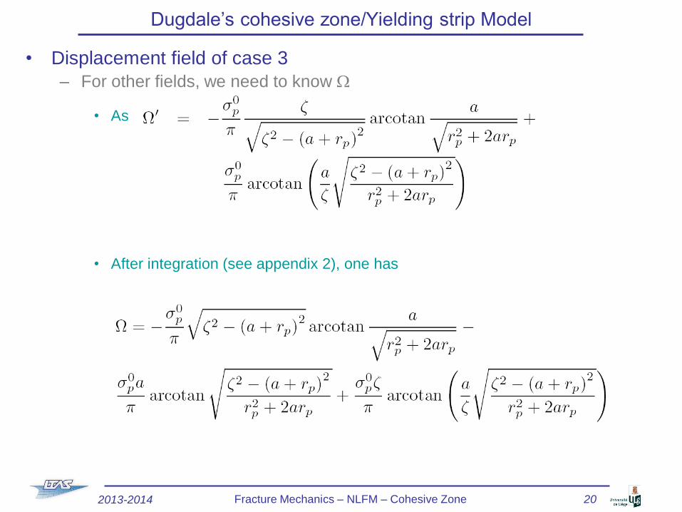
• Displacement field of case 3
– For other fields, we need to know W
• As
• After integration (see appendix 2), one has
Dugdale’s cohesive zone/Yielding strip Model
2013-2014 Fracture Mechanics – NLFM – Cohesive Zone 20
Dugdale’s cohesive zone/Yielding strip Model
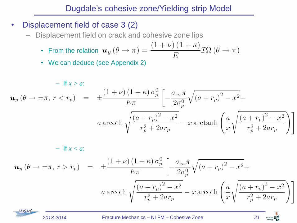
• Displacement field of case 3 (2)
– Displacement field on crack and cohesive zone lips
• From the relation
• We can deduce (see Appendix 2)
– If x > a:
– If x < a:
2013-2014 Fracture Mechanics – NLFM – Cohesive Zone 21
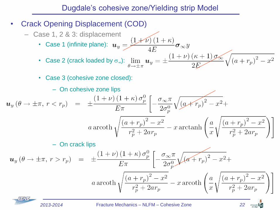
• Crack Opening Displacement (COD)
– Case 1, 2 & 3: displacement
• Case 1 (infinite plane):
• Case 2 (crack loaded by s∞):
• Case 3 (cohesive zone closed):
– On cohesive zone lips
– On crack lips
Dugdale’s cohesive zone/Yielding strip Model
2013-2014 Fracture Mechanics – NLFM – Cohesive Zone 22
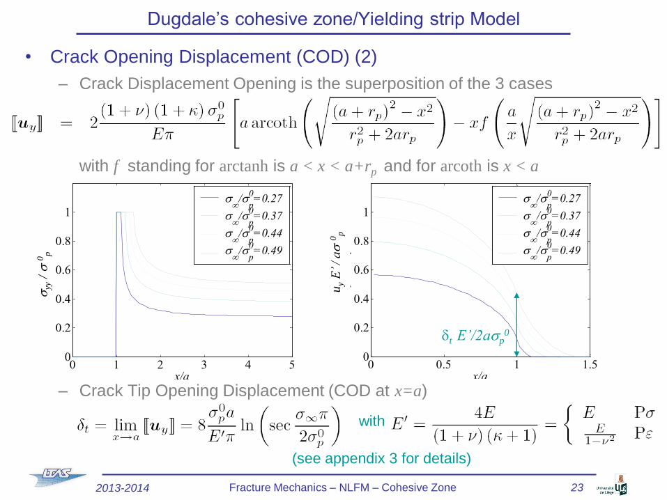
• Crack Opening Displacement (COD) (2)
– Crack Displacement Opening is the superposition of the 3 cases
with f standing for arctanh is a < x < a+rp and for arcoth is x < a
– Crack Tip Opening Displacement (COD at x=a)
with
(see appendix 3 for details)
Dugdale’s cohesive zone/Yielding strip Model
2013-2014 Fracture Mechanics – NLFM – Cohesive Zone 23
0 1 2 3 4 50
0.2
0.4
0.6
0.8
1
x/a
syy
/ sp0
s
/sp
0=0.27
s
/sp
0=0.37
s
/sp
0=0.44
s
/sp
0=0.49
syy
/ s
0p
0 0.5 1 1.50
0.2
0.4
0.6
0.8
1
x/a
uy E
'/a
sp0
s
/sp
0=0.27
s
/sp
0=0.37
s
/sp
0=0.44
s
/sp
0=0.49
dt E’/2asp0
uy
E’ /
as
0p
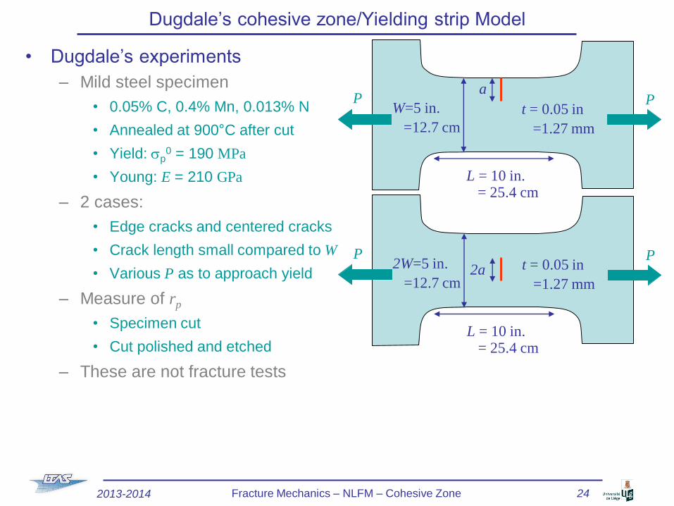
• Dugdale’s experiments
– Mild steel specimen
• 0.05% C, 0.4% Mn, 0.013% N
• Annealed at 900°C after cut
• Yield: sp0 = 190 MPa
• Young: E = 210 GPa
– 2 cases:
• Edge cracks and centered cracks
• Crack length small compared to W
• Various P as to approach yield
– Measure of rp
• Specimen cut
• Cut polished and etched
– These are not fracture tests
Dugdale’s cohesive zone/Yielding strip Model
a
W=5 in.
=12.7 cm
L = 10 in.= 25.4 cm
t = 0.05 in
=1.27 mm
P P
2a2W=5 in.
=12.7 cm
L = 10 in.= 25.4 cm
t = 0.05 in
=1.27 mm
P P
2013-2014 Fracture Mechanics – NLFM – Cohesive Zone 24
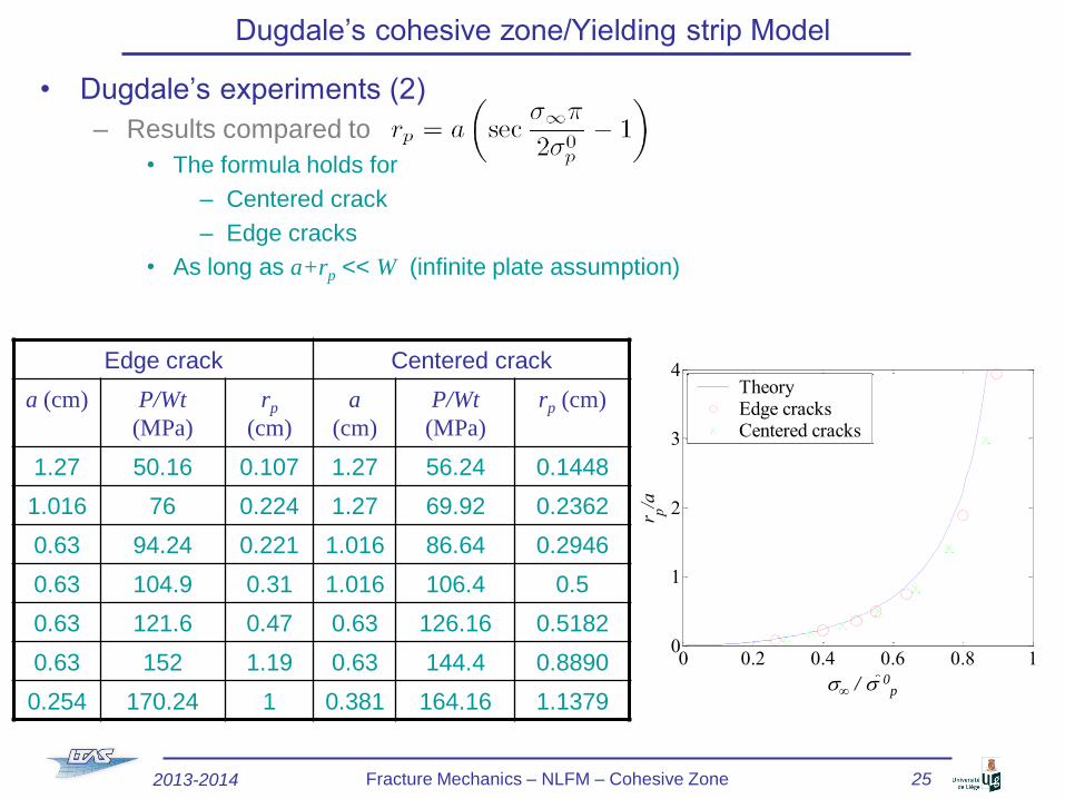
• Dugdale’s experiments (2)
– Results compared to
• The formula holds for
– Centered crack
– Edge cracks
• As long as a+rp << W (infinite plate assumption)
Dugdale’s cohesive zone/Yielding strip Model
Edge crack Centered crack
a (cm) P/Wt
(MPa)
rp
(cm)
a
(cm)
P/Wt
(MPa)
rp (cm)
1.27 50.16 0.107 1.27 56.24 0.1448
1.016 76 0.224 1.27 69.92 0.2362
0.63 94.24 0.221 1.016 86.64 0.2946
0.63 104.9 0.31 1.016 106.4 0.5
0.63 121.6 0.47 0.63 126.16 0.5182
0.63 152 1.19 0.63 144.4 0.8890
0.254 170.24 1 0.381 164.16 1.1379
2013-2014 Fracture Mechanics – NLFM – Cohesive Zone 25
0 0.2 0.4 0.6 0.8 10
1
2
3
4
s
/sp
0
r p/a
TheoryEdge cracksCentered cracks
s∞ / s 0p
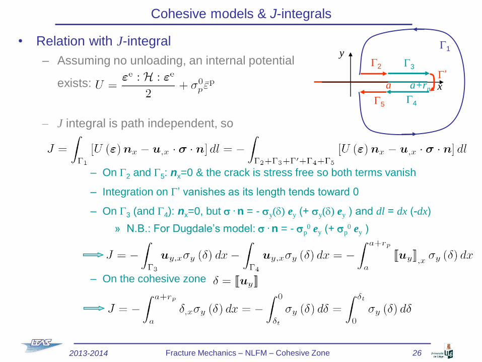
• Relation with J-integral
– Assuming no unloading, an internal potential
exists:
– J integral is path independent, so
– On G2 and G5: nx=0 & the crack is stress free so both terms vanish
– Integration on G’ vanishes as its length tends toward 0
– On G3 (and G4): nx=0, but s . n = - sy(d) ey (+ sy(d) ey ) and dl = dx (-dx)
» N.B.: For Dugdale’s model: s . n = - sp0 ey (+ sp
0 ey )
– On the cohesive zone
Cohesive models & J-integrals
a a+rp
y
x
G5
G1
G2 G3
G4
G’
2013-2014 Fracture Mechanics – NLFM – Cohesive Zone 26
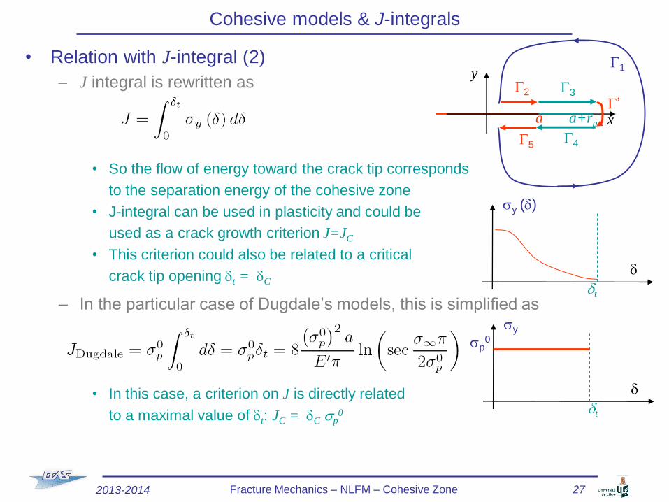
• Relation with J-integral (2)
– J integral is rewritten as
• So the flow of energy toward the crack tip corresponds
to the separation energy of the cohesive zone
• J-integral can be used in plasticity and could be
used as a crack growth criterion J=JC
• This criterion could also be related to a critical
crack tip opening dt = dC
– In the particular case of Dugdale’s models, this is simplified as
• In this case, a criterion on J is directly related
to a maximal value of dt: JC = dC sp0
Cohesive models & J-integrals
d
sy
sp0
dt
d
sy (d)
dt
a a+rp
y
x
G5
G1
G2 G3
G4
G’
2013-2014 Fracture Mechanics – NLFM – Cohesive Zone 27
• Can LEFM be extended to elastic perfectly plastic analysis?
– It is possible if there is no extensive plasticity prior to fracture
• Plastic zone small compared to characteristic lengths
– A criterion of crack growth might be J ≥ JC
– Are the SIFs still meaningful? If so how do we compute them?
– The extension is based on the use of an “effective crack length”
• Effective crack length with h a factor to be determined
• As we want to use LEFM, J is rewritten in terms of SIFs
– Mode I & infinite plane: &
– So the effective length is
Effective crack length
2013-2014 Fracture Mechanics – NLFM – Cohesive Zone 28

• Can LEFM be extended to elastic perfectly plastic analysis (2)?
– The extension is based on the use of an “effective crack length” (2)
• Mode I & infinite plane:
• If s∞< sp0
– As
– As
– Eventually, for SSY, h = 1/3
• CTOD can be computed from aeff as
Effective crack length
2013-2014 Fracture Mechanics – NLFM – Cohesive Zone 29
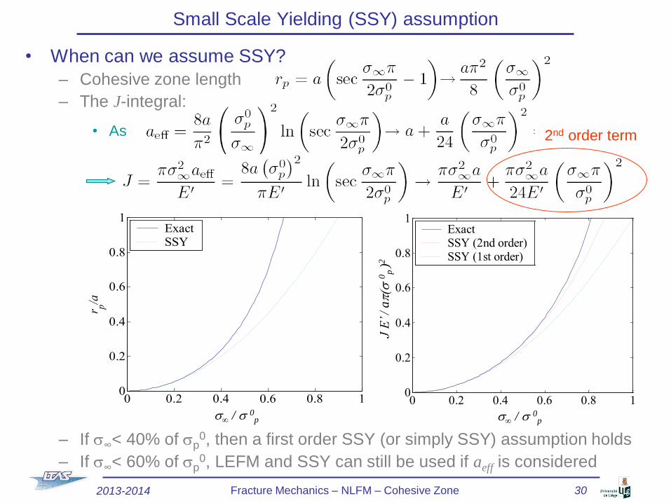
• When can we assume SSY?
– Cohesive zone length
– The J-integral:
• As
– If s∞< 40% of sp0, then a first order SSY (or simply SSY) assumption holds
– If s∞< 60% of sp0, LEFM and SSY can still be used if aeff is considered
Small Scale Yielding (SSY) assumption
0 0.2 0.4 0.6 0.8 10
0.2
0.4
0.6
0.8
1
s
/sp
0
r p/a
ExactSSY
2nd order term
2013-2014 Fracture Mechanics – NLFM – Cohesive Zone 30
s∞ / s 0p
0 0.2 0.4 0.6 0.8 10
0.2
0.4
0.6
0.8
1
s
/sp
0
J E
'/a
(
sp0)2
ExactSSY (2nd order)SSY (1st order)
s∞ / s 0p
J E
’ /
a
(s 0
p )
2
• SSY (first order) for Dugdale’s model
– If s∞< 40% of sp0 then a first order SSY (or simply SSY) assumption holds
• The cohesive zone is limited (rp < 20% of a)
• For a infinite plate in mode I, the J-integral is reduced to
SIFs concept of LEFM holds (without correction of the crack size)
• Size of the plastic (cohesive zone)
• As SSY requires rp < 20% of a, elastic fracture criterion can be applied if
– So crack length has to be large enough compared to the plastic zone
– The method is actually applicable if the plastic zone is small compared to
» The crack (a> 5 rp)
» The distance from the crack tip to the nearest free surface (L > 5 rp)
• If we are well before fracture (beginning of fatigue e.g.), we do not have to use KC
Small Scale Yielding (SSY) assumption
2013-2014 Fracture Mechanics – NLFM – Cohesive Zone 31
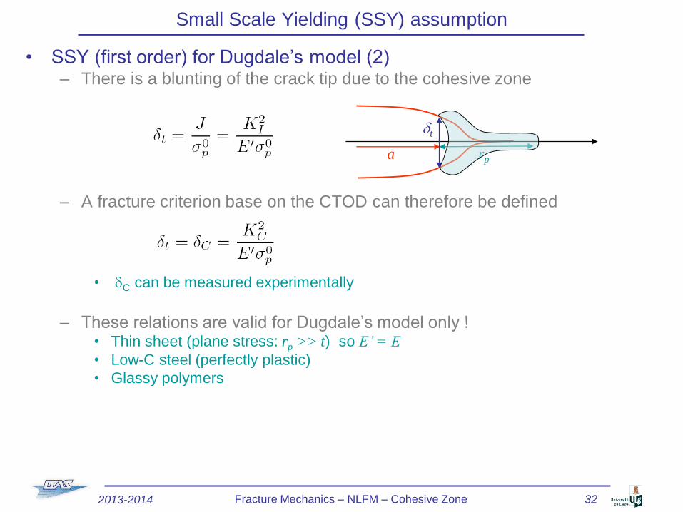
• SSY (first order) for Dugdale’s model (2)– There is a blunting of the crack tip due to the cohesive zone
– A fracture criterion base on the CTOD can therefore be defined
• dC can be measured experimentally
– These relations are valid for Dugdale’s model only !• Thin sheet (plane stress: rp >> t) so E’ = E
• Low-C steel (perfectly plastic)
• Glassy polymers
Small Scale Yielding (SSY) assumption
a rp
dt
2013-2014 Fracture Mechanics – NLFM – Cohesive Zone 32
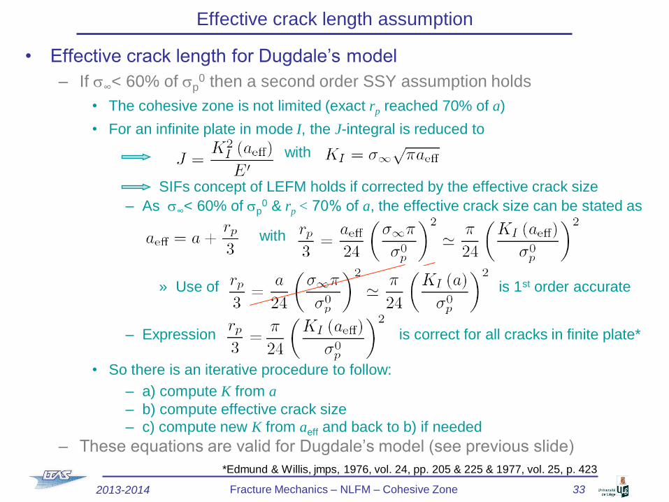
• Effective crack length for Dugdale’s model
– If s∞< 60% of sp0 then a second order SSY assumption holds
• The cohesive zone is not limited (exact rp reached 70% of a)
• For an infinite plate in mode I, the J-integral is reduced to
with
SIFs concept of LEFM holds if corrected by the effective crack size
– As s∞< 60% of sp0 & rp < 70% of a, the effective crack size can be stated as
with
» Use of is 1st order accurate
– Expression is correct for all cracks in finite plate*
• So there is an iterative procedure to follow:
– a) compute K from a
– b) compute effective crack size
– c) compute new K from aeff and back to b) if needed
– These equations are valid for Dugdale’s model (see previous slide)
Effective crack length assumption
*Edmund & Willis, jmps, 1976, vol. 24, pp. 205 & 225 & 1977, vol. 25, p. 423
2013-2014 Fracture Mechanics – NLFM – Cohesive Zone 33
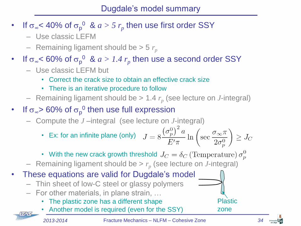
• If s∞< 40% of sp0 & a > 5 rp then use first order SSY
– Use classic LEFM
– Remaining ligament should be > 5 rp
• If s∞< 60% of sp0 & a > 1.4 rp then use a second order SSY
– Use classic LEFM but
• Correct the crack size to obtain an effective crack size
• There is an iterative procedure to follow
– Remaining ligament should be > 1.4 rp (see lecture on J-integral)
• If s∞> 60% of sp0 then use full expression
– Compute the J –integral (see lecture on J-integral)
• Ex: for an infinite plane (only)
• With the new crack growth threshold
– Remaining ligament should be > rp (see lecture on J-integral)
• These equations are valid for Dugdale’s model– Thin sheet of low-C steel or glassy polymers
– For other materials, in plane strain, …• The plastic zone has a different shape
• Another model is required (even for the SSY)
Dugdale’s model summary
Plastic
zone
2013-2014 Fracture Mechanics – NLFM – Cohesive Zone 34
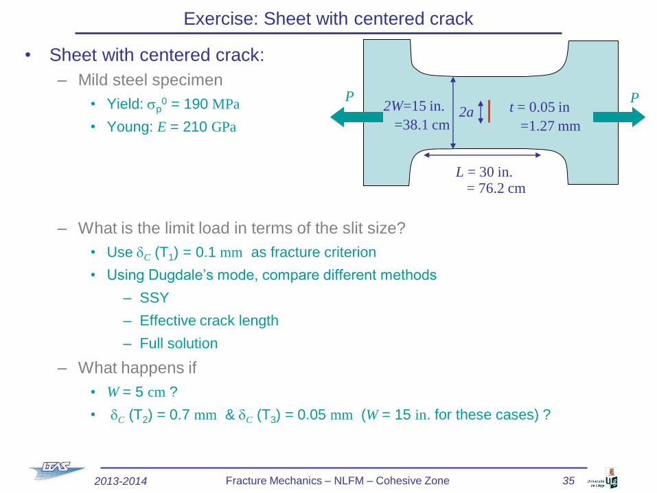
• Sheet with centered crack:
– Mild steel specimen
• Yield: sp0 = 190 MPa
• Young: E = 210 GPa
– What is the limit load in terms of the slit size?
• Use dC (T1) = 0.1 mm as fracture criterion
• Using Dugdale’s mode, compare different methods
– SSY
– Effective crack length
– Full solution
– What happens if
• W = 5 cm ?
• dC (T2) = 0.7 mm & dC (T3) = 0.05 mm (W = 15 in. for these cases) ?
Exercise: Sheet with centered crack
2a2W=15 in.
=38.1 cm
L = 30 in.= 76.2 cm
t = 0.05 in
=1.27 mm
P P
2013-2014 Fracture Mechanics – NLFM – Cohesive Zone 35
References
• Lecture notes
– Lecture Notes on Fracture Mechanics, Alan T. Zehnder, Cornell University,
Ithaca, http://hdl.handle.net/1813/3075
• Other references
– « on-line »
• Fracture Mechanics, Piet Schreurs, TUe, http://www.mate.tue.nl/~piet/edu/frm/sht/bmsht.html
– Book
• Fracture Mechanics: Fundamentals and applications, D. T. Anderson. CRC press, 1991.
• Fatigue of Materials, S. Suresh, Cambridge press, 1998.
2013-2014 Fracture Mechanics – NLFM – Cohesive Zone 36
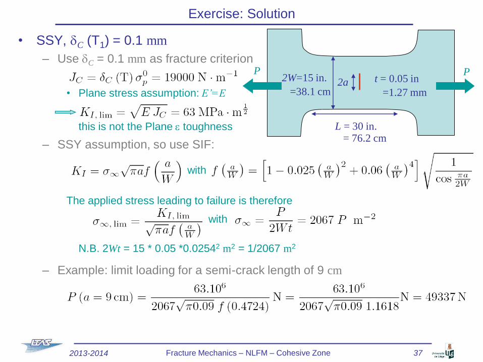
• SSY, dC (T1) = 0.1 mm
– Use dC = 0.1 mm as fracture criterion
• Plane stress assumption: E’=E
this is not the Plane e toughness
– SSY assumption, so use SIF:
with
The applied stress leading to failure is therefore
with
N.B. 2Wt = 15 * 0.05 *0.02542 m2 = 1/2067 m2
– Example: limit loading for a semi-crack length of 9 cm
Exercise: Solution
2a2W=15 in.
=38.1 cm
L = 30 in.= 76.2 cm
t = 0.05 in
=1.27 mm
P P
2013-2014 Fracture Mechanics – NLFM – Cohesive Zone 37
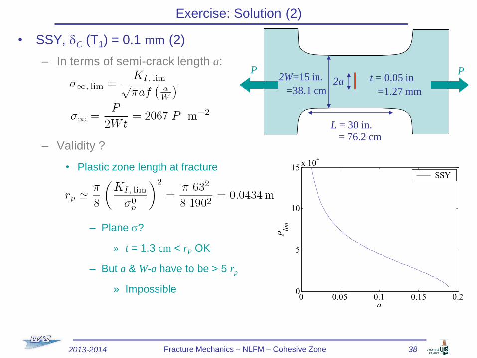
• SSY, dC (T1) = 0.1 mm (2)
– In terms of semi-crack length a:
– Validity ?
• Plastic zone length at fracture
– Plane s?
» t = 1.3 cm < rP OK
– But a & W-a have to be > 5 rp
» Impossible
Exercise: Solution (2)
0 0.05 0.1 0.15 0.20
5
10
15x 10
4
a
Pli
m
SSY
2a2W=15 in.
=38.1 cm
L = 30 in.= 76.2 cm
t = 0.05 in
=1.27 mm
P P
2013-2014 Fracture Mechanics – NLFM – Cohesive Zone 38
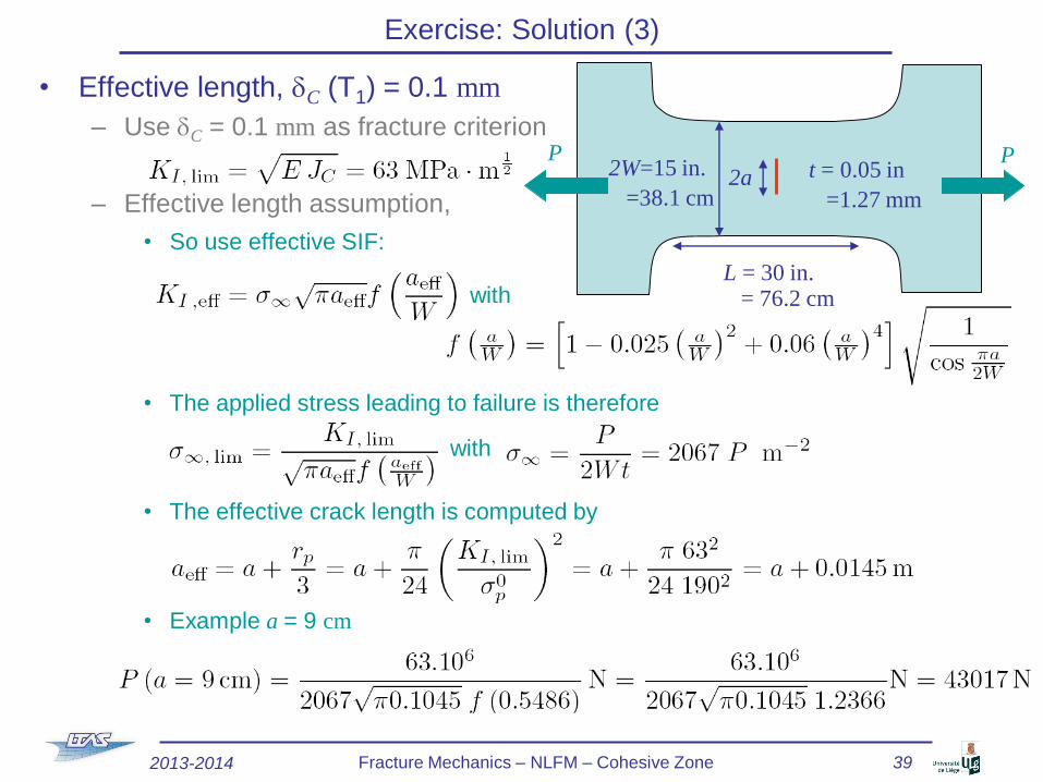
• Effective length, dC (T1) = 0.1 mm
– Use dC = 0.1 mm as fracture criterion
– Effective length assumption,
• So use effective SIF:
with
• The applied stress leading to failure is therefore
with
• The effective crack length is computed by
• Example a = 9 cm
Exercise: Solution (3)
2a2W=15 in.
=38.1 cm
L = 30 in.= 76.2 cm
t = 0.05 in
=1.27 mm
P P
2013-2014 Fracture Mechanics – NLFM – Cohesive Zone 39
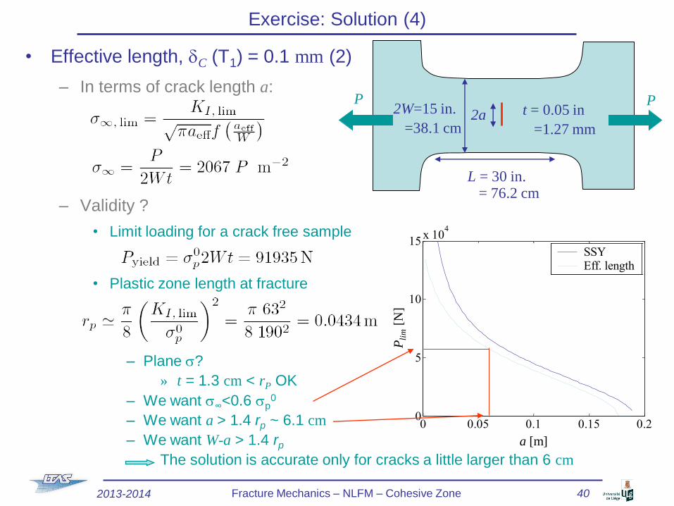
• Effective length, dC (T1) = 0.1 mm (2)
– In terms of crack length a:
– Validity ?
• Limit loading for a crack free sample
• Plastic zone length at fracture
– Plane s?
» t = 1.3 cm < rP OK
– We want s∞<0.6 sp0
– We want a > 1.4 rp ~ 6.1 cm
– We want W-a > 1.4 rp
The solution is accurate only for cracks a little larger than 6 cm
Exercise: Solution (4)
0 0.05 0.1 0.15 0.20
5
10
15x 10
4
a
Pli
m
SSYEff. length
a [m]
Pli
m[N
]
2a2W=15 in.
=38.1 cm
L = 30 in.= 76.2 cm
t = 0.05 in
=1.27 mm
P P
2013-2014 Fracture Mechanics – NLFM – Cohesive Zone 40
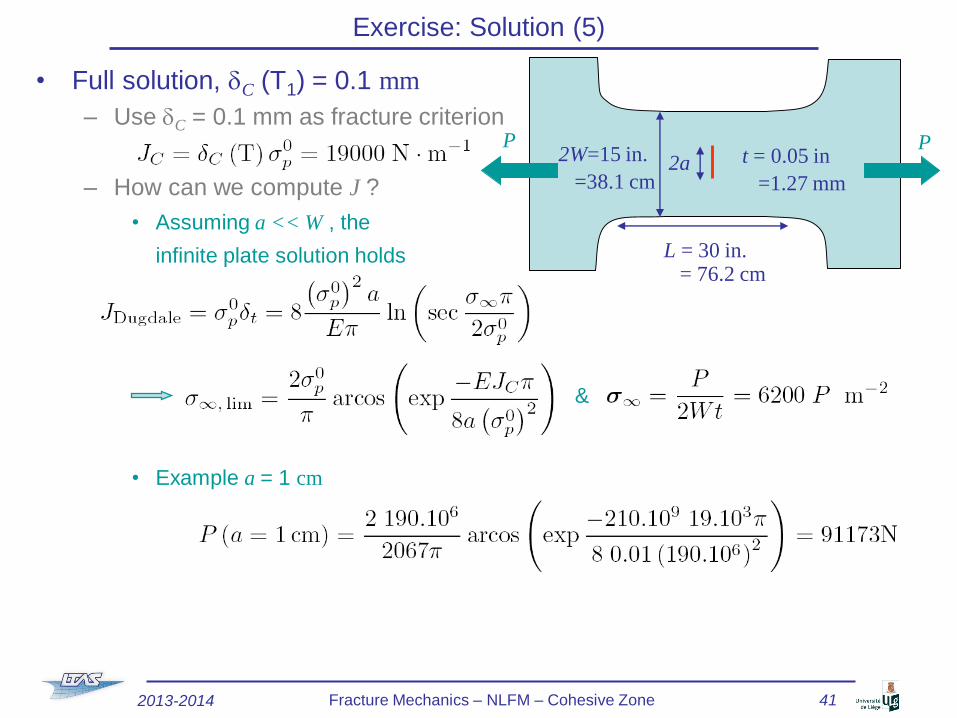
• Full solution, dC (T1) = 0.1 mm
– Use dC = 0.1 mm as fracture criterion
– How can we compute J ?
• Assuming a << W , the
infinite plate solution holds
&
• Example a = 1 cm
Exercise: Solution (5)
2a2W=15 in.
=38.1 cm
L = 30 in.= 76.2 cm
t = 0.05 in
=1.27 mm
P P
2013-2014 Fracture Mechanics – NLFM – Cohesive Zone 41
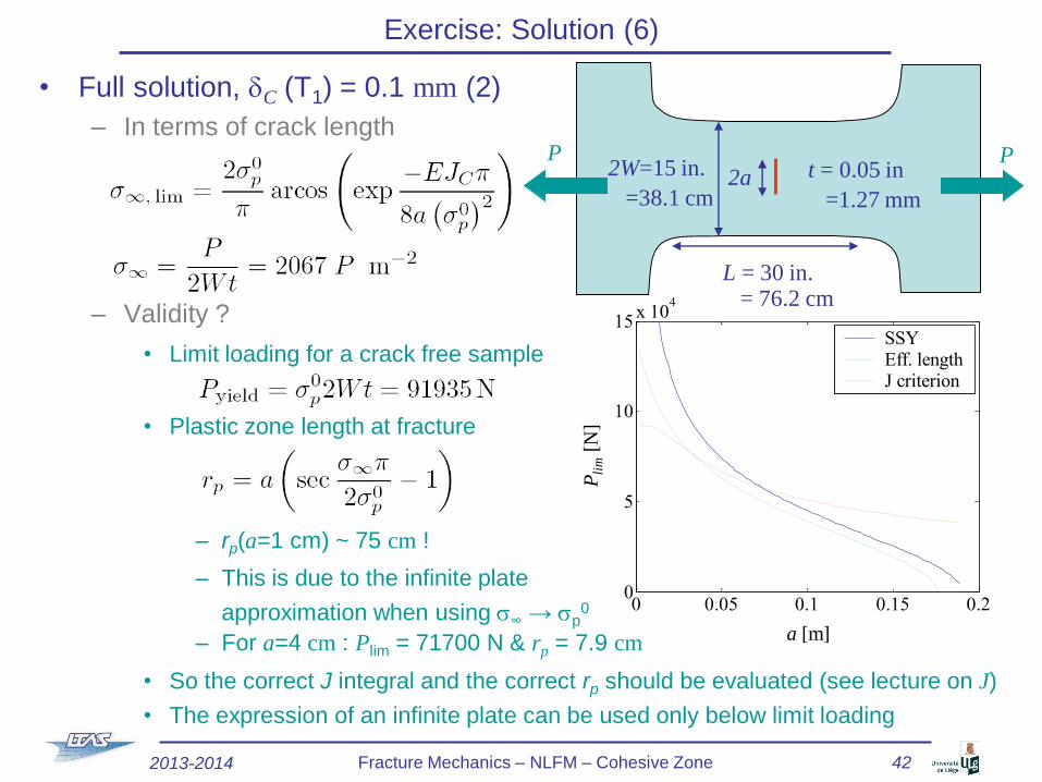
• Full solution, dC (T1) = 0.1 mm (2)
– In terms of crack length
&
– Validity ?
• Limit loading for a crack free sample
• Plastic zone length at fracture
– rp(a=1 cm) ~ 75 cm !
– This is due to the infinite plate
approximation when using s∞ → sp0
– For a=4 cm : Plim = 71700 N & rp = 7.9 cm
• So the correct J integral and the correct rp should be evaluated (see lecture on J)
• The expression of an infinite plate can be used only below limit loading
Exercise: Solution (6)
2a2W=15 in.
=38.1 cm
L = 30 in.= 76.2 cm
t = 0.05 in
=1.27 mm
P P
2013-2014 Fracture Mechanics – NLFM – Cohesive Zone 42
0 0.05 0.1 0.15 0.20
5
10
15x 10
4
a
Pli
m
SSYEff. lengthJ criterion
a [m]
Pli
m[N
]
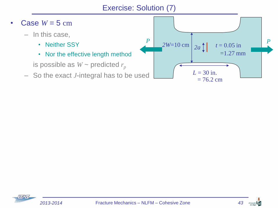
• Case W = 5 cm
– In this case,
• Neither SSY
• Nor the effective length method
is possible as W ~ predicted rp
– So the exact J-integral has to be used
Exercise: Solution (7)
2a2W=10 cm
L = 30 in.= 76.2 cm
t = 0.05 in
=1.27 mm
P P
2013-2014 Fracture Mechanics – NLFM – Cohesive Zone 43
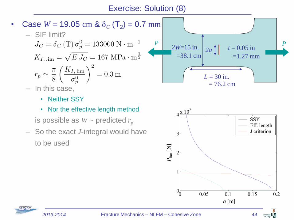
• Case W = 19.05 cm & dC (T2) = 0.7 mm
– SIF limit?
– In this case,
• Neither SSY
• Nor the effective length method
is possible as W ~ predicted rp
– So the exact J-integral would have
to be used
Exercise: Solution (8)
2a2W=15 in.
=38.1 cm
L = 30 in.= 76.2 cm
t = 0.05 in
=1.27 mm
P P
2013-2014 Fracture Mechanics – NLFM – Cohesive Zone 44
0 0.05 0.1 0.15 0.20
1
2
3
4x 10
5
a
Pli
m
SSYEff. lengthJ criterion
a [m]
Pli
m[N
]
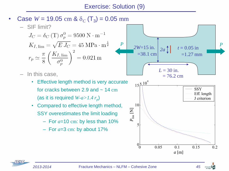
• Case W = 19.05 cm & dC (T3) = 0.05 mm
– SIF limit?
– In this case,
• Effective length method is very accurate
for cracks between 2.9 and ~ 14 cm
(as it is required W-a>1.4 rp)
• Compared to effective length method,
SSY overestimates the limit loading
– For a=10 cm: by less than 10%
– For a=3 cm: by about 17%
Exercise: Solution (9)
2a2W=15 in.
=38.1 cm
L = 30 in.= 76.2 cm
t = 0.05 in
=1.27 mm
P P
2013-2014 Fracture Mechanics – NLFM – Cohesive Zone 45
0 0.05 0.1 0.15 0.20
5
10
15x 10
4
a
Pli
m
SSYEff. lengthJ criterion
a [m]
Pli
m[N
]
• For ductile materials
– SSY is almost never a good
approximation
• The plastic zone is too large compared to crack size and remaining ligament
• Except in very low loading
– Effective length scale
• Can be used for
– Critical loading estimation
» For large specimen and
» If crack length is in a specific range
– Computation of SIF for fatigue
» As K is reduced, the plastic zone size is reduced
» So the crack length validity range is increased
– J-integral can be used, but
• The infinite plane approximation is a good approximation only
– If loading < 90% of yield
– Crack size and plastic zone size << W
• Exact solution can be computed (see lecture on J-integral)
Exercise: Summary
2013-2014 Fracture Mechanics – NLFM – Cohesive Zone 46
2a
x
y
rprp
sp0 sp
0
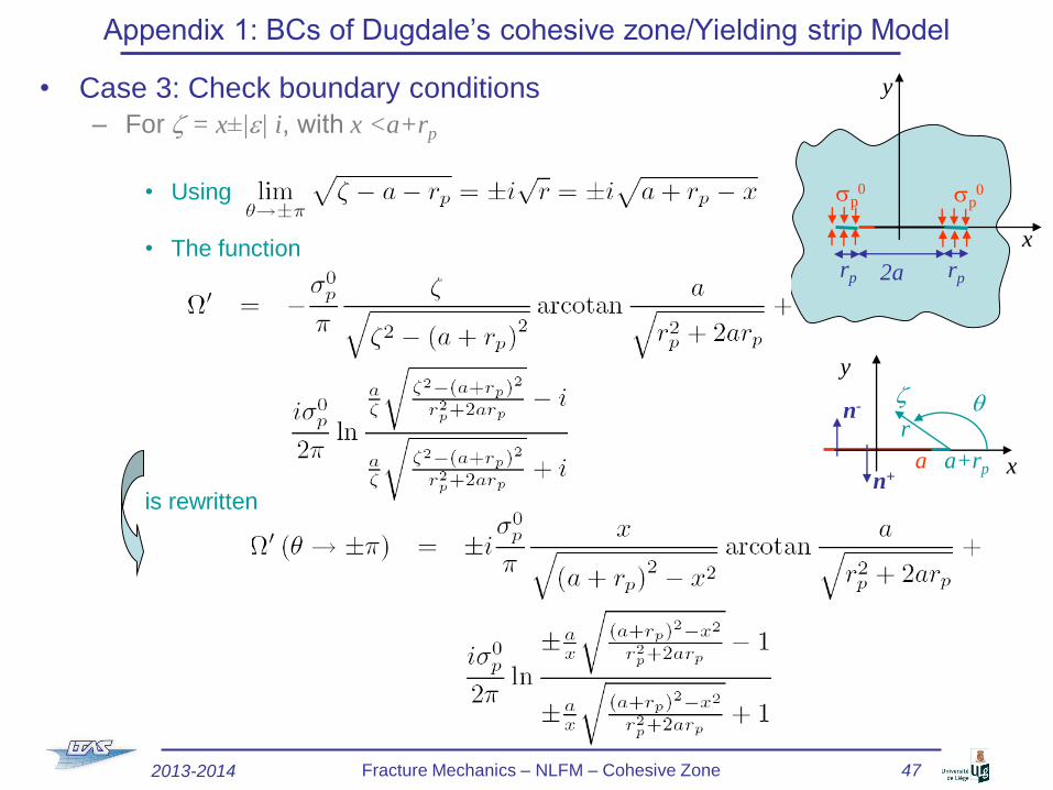
Appendix 1: BCs of Dugdale’s cohesive zone/Yielding strip Model
• Case 3: Check boundary conditions
– For z = x±|e| i, with x <a+rp
• Using
• The function
is rewritten
a a+rp
y
x
qr
z
n+
n-
2013-2014 Fracture Mechanics – NLFM – Cohesive Zone 47
2a
x
y
rprp
sp0 sp
0
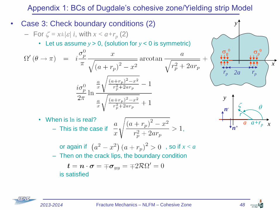
• Case 3: Check boundary conditions (2)
– For z = x±|e| i, with x < a+rp (2)
• Let us assume y > 0, (solution for y < 0 is symmetric)
• When is ln is real?
– This is the case if ,
or again if , so if x < a
– Then on the crack lips, the boundary condition
is satisfied
Appendix 1: BCs of Dugdale’s cohesive zone/Yielding strip Model
a a+rp
y
x
qr
z
n+
n-
2013-2014 Fracture Mechanics – NLFM – Cohesive Zone 48
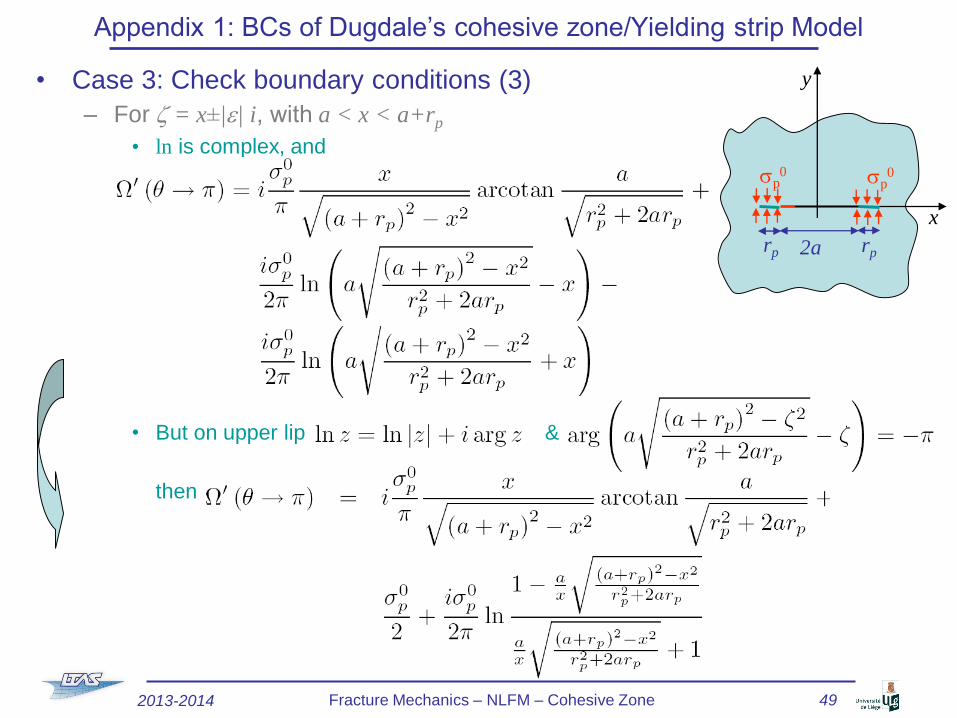
Appendix 1: BCs of Dugdale’s cohesive zone/Yielding strip Model
• Case 3: Check boundary conditions (3)
– For z = x±|e| i, with a < x < a+rp
• ln is complex, and
• But on upper lip &
then
2a
x
y
rprp
sp0 sp
0
2013-2014 Fracture Mechanics – NLFM – Cohesive Zone 49
2a
x
y
rprp
sp0 sp
0
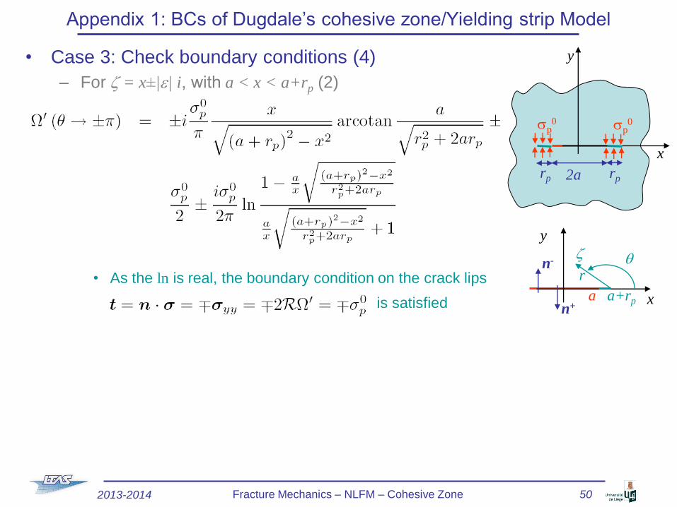
• Case 3: Check boundary conditions (4)
– For z = x±|e| i, with a < x < a+rp (2)
• As the ln is real, the boundary condition on the crack lips
is satisfied
Appendix 1: BCs of Dugdale’s cohesive zone/Yielding strip Model
a a+rp
y
x
qr
z
n+
n-
2013-2014 Fracture Mechanics – NLFM – Cohesive Zone 50
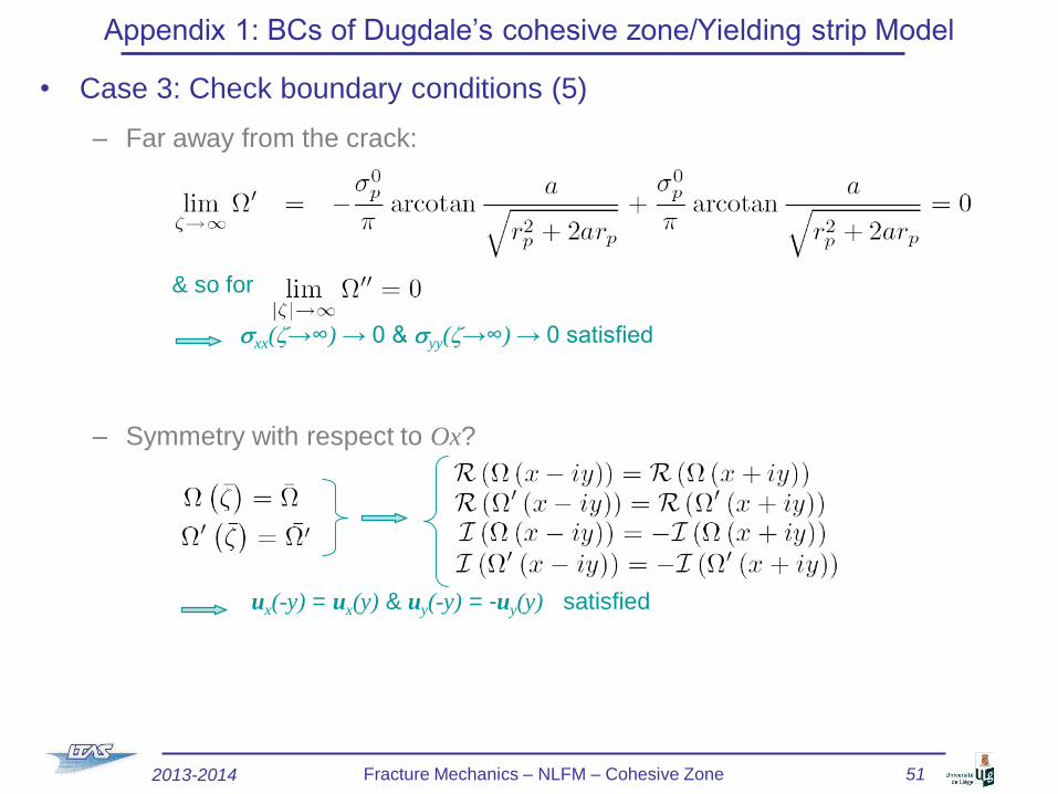
• Case 3: Check boundary conditions (5)
– Far away from the crack:
& so for
sxx(z→∞) → 0 & syy(z→∞) → 0 satisfied
– Symmetry with respect to Ox?
ux(-y) = ux(y) & uy(-y) = -uy(y) satisfied
Appendix 1: BCs of Dugdale’s cohesive zone/Yielding strip Model
2013-2014 Fracture Mechanics – NLFM – Cohesive Zone 51
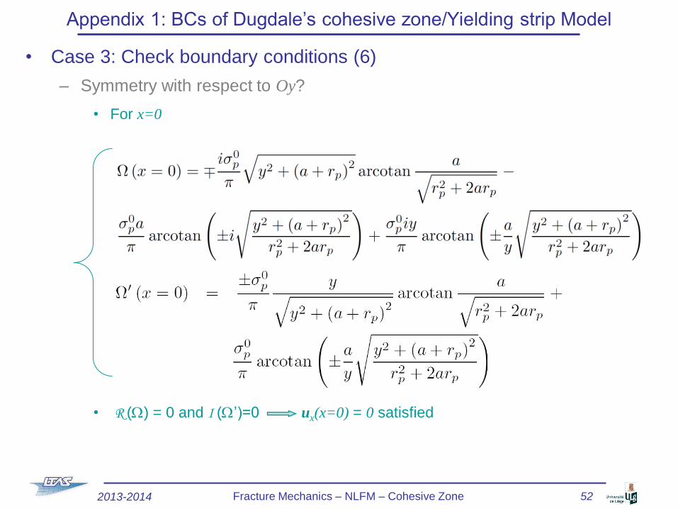
• Case 3: Check boundary conditions (6)
– Symmetry with respect to Oy?
• For x=0
• R (W) = 0 and I (W’)=0 ux(x=0) = 0 satisfied
Appendix 1: BCs of Dugdale’s cohesive zone/Yielding strip Model
2013-2014 Fracture Mechanics – NLFM – Cohesive Zone 52
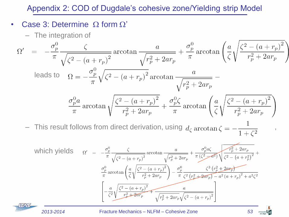
Appendix 2: COD of Dugdale’s cohesive zone/Yielding strip Model
• Case 3: Determine W form W’
– The integration of
leads to
– This result follows from direct derivation, using ,
which yields
2013-2014 Fracture Mechanics – NLFM – Cohesive Zone 53
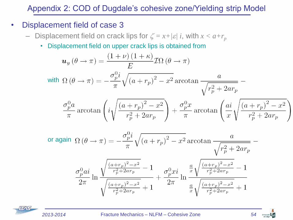
• Displacement field of case 3
– Displacement field on crack lips for z = x+|e| i, with x < a+rp
• Displacement field on upper crack lips is obtained from
with
or again
Appendix 2: COD of Dugdale’s cohesive zone/Yielding strip Model
2013-2014 Fracture Mechanics – NLFM – Cohesive Zone 54
• Displacement field of case 3 (2)
– Displacement field for z = x+|e| i, with x < a+rp (2)
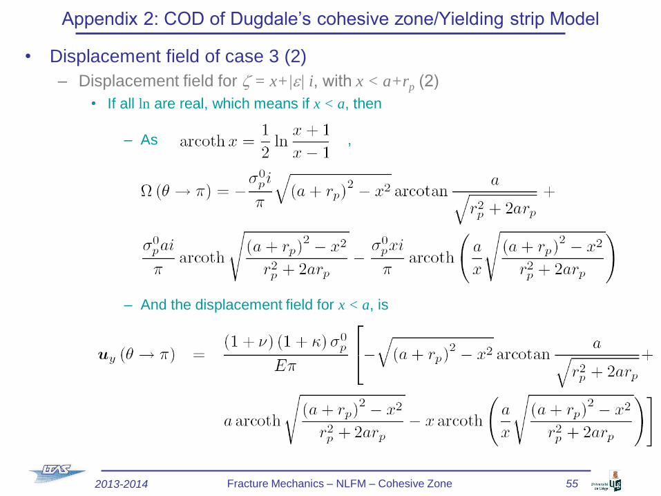
• If all ln are real, which means if x < a, then
– As ,
– And the displacement field for x < a, is
Appendix 2: COD of Dugdale’s cohesive zone/Yielding strip Model
2013-2014 Fracture Mechanics – NLFM – Cohesive Zone 55
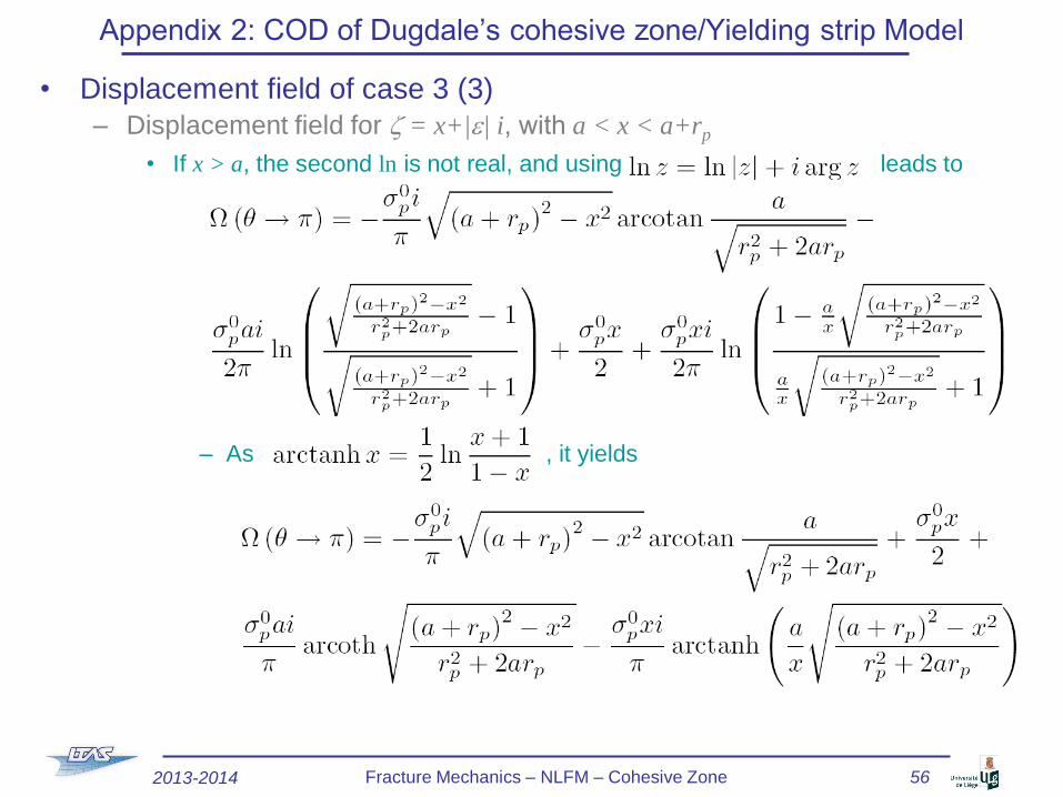
• Displacement field of case 3 (3)
– Displacement field for z = x+|e| i, with a < x < a+rp
• If x > a, the second ln is not real, and using leads to
– As , it yields
Appendix 2: COD of Dugdale’s cohesive zone/Yielding strip Model
2013-2014 Fracture Mechanics – NLFM – Cohesive Zone 56
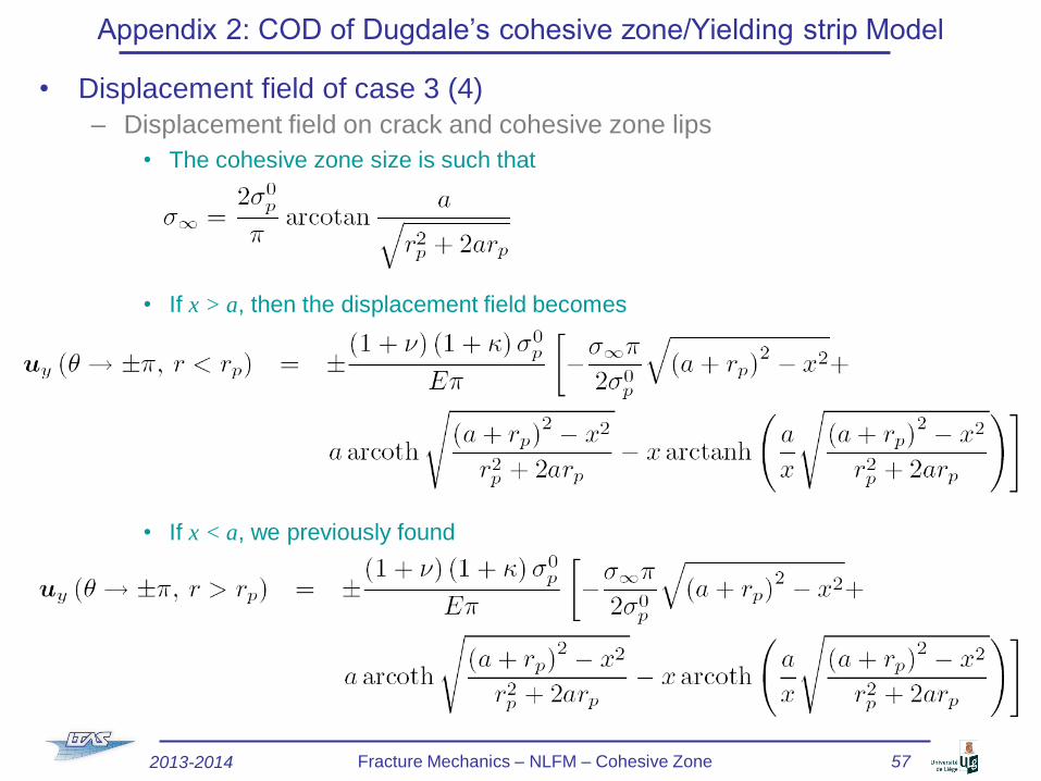
• Displacement field of case 3 (4)
– Displacement field on crack and cohesive zone lips
• The cohesive zone size is such that
• If x > a, then the displacement field becomes
• If x < a, we previously found
Appendix 2: COD of Dugdale’s cohesive zone/Yielding strip Model
2013-2014 Fracture Mechanics – NLFM – Cohesive Zone 57
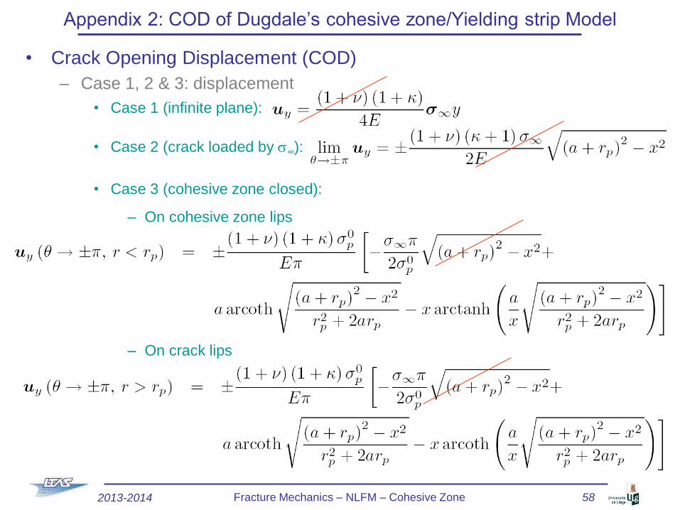
• Crack Opening Displacement (COD)
– Case 1, 2 & 3: displacement
• Case 1 (infinite plane):
• Case 2 (crack loaded by s∞):
• Case 3 (cohesive zone closed):
– On cohesive zone lips
– On crack lips
Appendix 2: COD of Dugdale’s cohesive zone/Yielding strip Model
2013-2014 Fracture Mechanics – NLFM – Cohesive Zone 58
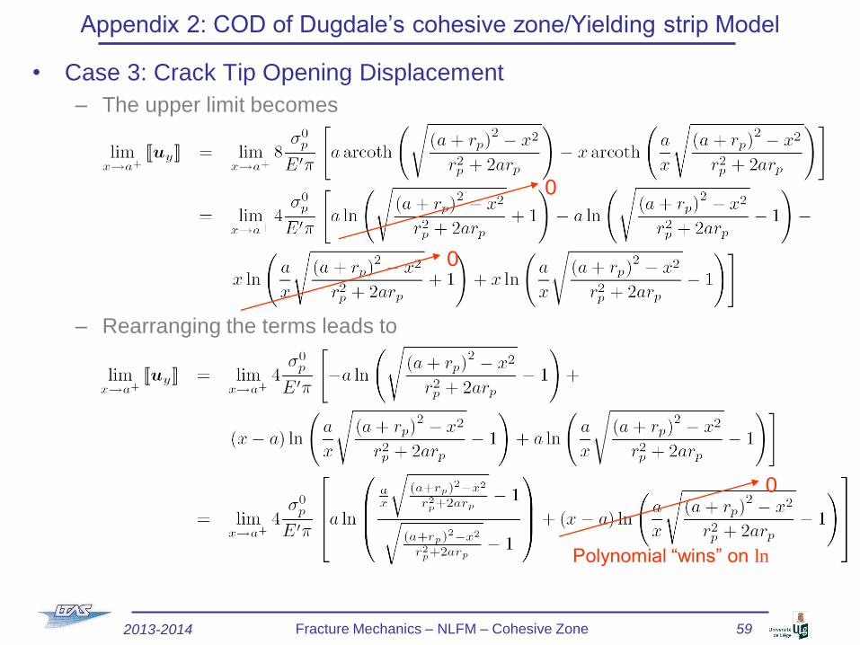
• Case 3: Crack Tip Opening Displacement
– The upper limit becomes
– Rearranging the terms leads to
0
0
0
Polynomial “wins” on ln
Appendix 2: COD of Dugdale’s cohesive zone/Yielding strip Model
2013-2014 Fracture Mechanics – NLFM – Cohesive Zone 59
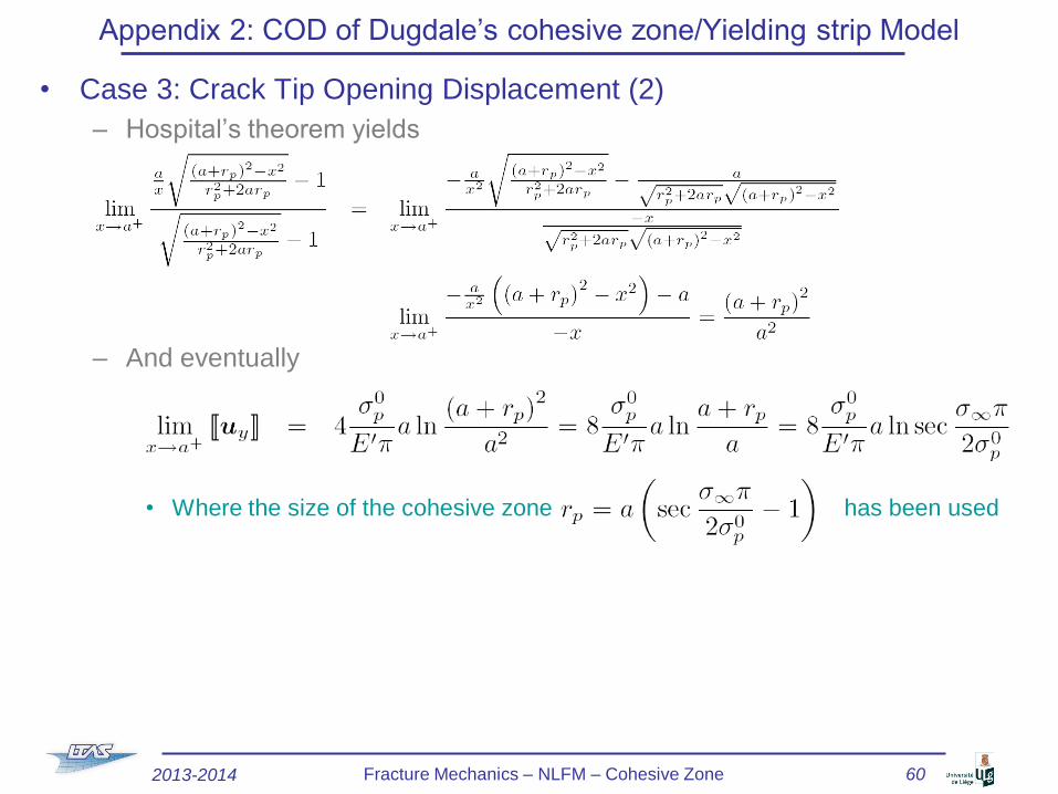
• Case 3: Crack Tip Opening Displacement (2)
– Hospital’s theorem yields
– And eventually
• Where the size of the cohesive zone has been used
Appendix 2: COD of Dugdale’s cohesive zone/Yielding strip Model
2013-2014 Fracture Mechanics – NLFM – Cohesive Zone 60